Limited-control optimal protocols arbitrarily far from equilibrium

Abstract

Recent studies have explored finite-time dissipation-minimizing protocols for stochastic thermodynamic systems driven arbitrarily far from equilibrium, when granted full external control to drive the system. However, in both simulation and experimental contexts, systems often may only be controlled with a limited set of degrees of freedom. Here, going beyond slow- and fast-driving approximations employed in previous studies, we obtain exact finite-time optimal protocols for this unexplored limited-control setting. By working with deterministic Fokker-Planck probability density time evolution, we can frame the work-minimizing protocol problem in the standard form of an optimal control theory problem. We demonstrate that finding the exact optimal protocol is equivalent to solving a system of Hamiltonian partial differential equations, which in many cases admit efficiently calculatable numerical solutions. Within this framework, we reproduce analytical results for the optimal control of harmonic potentials, and numerically devise novel optimal protocols for two anharmonic examples: varying the stiffness of a quartic potential, and linearly biasing a double-well potential. We confirm that these optimal protocols outperform other protocols produced through previous methods, in some cases by a substantial amount. We find that for the linearly biased double-well problem, the mean position under the optimal protocol travels at a near-constant velocity. Surprisingly, for a certain timescale and barrier height regime, the optimal protocol is also non-monotonic in time.

I Introduction

There has been much recent progress in the study of non-equilibrium stochastic thermodynamics Seifert (2012); Jarzynski et al. (2013); Ciliberto (2017). In particular, optimal finite-time protocols have been derived for a variety of systems, with applications to finite-time free-energy difference estimation Schmiedl and Seifert (2007); Blaber and Sivak (2020); Gomez-Marin et al. (2008) engineering optimal bit erasure Proesmans et al. (2020); Zulkowski and DeWeese (2014), and the design of optimal nanoscale heat engines Blickle and Bechinger (2012); Frim and DeWeese (2021a, b).

For finite-time dissipation-minimizing protocols, there are two related optimization problems that are typically studied: designing protocols that transition between two specified distributions within finite time that minimize entropy production Aurell et al. (2011); Dechant and Sakurai (2019); Nakazato and Ito (2021); Chen et al. (2019), and designing protocols that minimize the amount work needed to shift between two different potential energy landscapes within finite time Schmiedl and Seifert (2007); Sivak and Crooks (2012). For the first problem, methods have been devised to fully control probability density evolution arbitrarily far from equilibrium Frim et al. (2021); Ilker et al. (2021); Martínez et al. (2016), establishing deep ties with optimal transport theory Aurell et al. (2011); Villani (2009); Dechant and Sakurai (2019) and culminating in the derivation of an absolute geometric lower bound for finite-time entropy production in terms of the $L^{2}$-Wasserstein distance Dechant and Sakurai (2019); Nakazato and Ito (2021); Chen et al. (2019); Chennakesavalu and Rotskoff (2022). Crucially, however, full control over the potential energy is needed to satisfy arbitrarily specified initial and terminal conditions for this problem.

Here, we consider the second problem for the case in which there is only limited, finite-dimensional control of the potential. Only for the simplest case of a Brownian particle in a harmonic potential has the fully non-equilibrium optimal protocol been analytically solved and studied Schmiedl and Seifert (2007); Aurell et al. (2011); Then and Engel (2008); Plata et al. (2019). For arbitrary potentials, limited control optimal protocol approximations for the slow near-equilibrium $t_{f}\gg 1$ Sivak and Crooks (2012, 2016); Zulkowski et al. (2012); Rotskoff and Crooks (2015); Lucero et al. (2019); Deffner and Bonança (2020); Abiuso et al. (2022) and the fast $t_{f}\ll 1$ Blaber et al. (2021) regimes have been derived, but these approximations generally are optimal only within the specified limits. Very recently, gradient methods have been devised to calculate fully non-equilibrium optimal protocols through sampling many stochastic trajectories Engel et al. (2022); Yan et al. (2022); Das et al. (2022).

In this work, we show that optimal control theory is a principled and powerful framework to derive exact optimal protocols for limited-control potentials arbitrarily far from equilibrium. Optimal control theory (OCT), having roots in Lagrange’s calculus of variations, is a well-studied field of applied mathematics that deals with finding controls of a dynamical system that optimize a specified objective function, with numerous applications to science and engineering Liberzon (2011); Lenhart and Workman (2007), including experimental physics Bechhoefer (2021). By working directly with the probability density undergoing deterministic Fokker-Planck dynamics (as opposed to individual stochastic trajectories), and rewriting the objective function using the first law of thermodynamics, we show that the problem of finding optimal protocols can be recast in the standard OCT problem form. We may then apply Pontryagin’s maximum principle, one of OCT’s foundational theorems, to yield Hamiltonian partial differential equations whose solutions directly give optimal protocols. We note that the optimal control of fields and stochastic systems has been previously studied within applied mathematics and engineering literature Bakshi and Theodorou (2020); Annunziato and Borzì (2013); Fattorini et al. (1999); Palmer and Milutinović (2011); Evans et al. (2021); Theodorou and Todorov (2012); Fleig and Guglielmi (2017); Annunziato and Borzi (2010); Popescu et al. (2010); Chernyak et al. (2013), but to our knowledge it has never been used to derive exact optimal work-minimizing protocols in stochastic thermodynamics.

An outline of this paper is as follows. First, we use OCT to derive Hamiltonian partial differential equations whose solutions give optimal protocols for the cases of Markov jump processes over discrete states and Langevin dynamics over continuous configuration space. We then solve these equations analytically for harmonic potential control to reproduce known optimal protocols. Finally, we describe and use a computationally efficient algorithm to numerically calculate optimal protocols for two anharmonic examples: controlling the stiffness of a quartic trap, and linearly biasing a quartic double-well potential. We demonstrate the superiority in performance of these optimal protocols compared to the protocols derived through approximation methods. We discover that for the linearly biased double-well problem, the mean position travels with near-constant velocity under the optimal protocol, and that certain optimal protocols have a remarkably counter-intuitive property — the control parameter is non-monotonic in time within a certain time and barrier height parameter regime. Finally, we discuss our findings and the implications of our work for the study of non-equilibrium stochastic thermodynamics.

II Discrete state derivation

We start by considering a continuous-time Markov jump process with $d$ discrete states. The experimenter has control over the protocol parameter $\lambda(t)$ that determines the potential energies of the states, encoded by the vector ${\bm{U}}_{\lambda}=(U_{1}(\lambda),U_{2}(\lambda),...,U_{d}(\lambda)))^{T}$. Here $\lambda$ is single parameter, but in general it can be multi-dimensional. Although an individual jump process trajectory is stochastic, the time-varying probability distribution over states, represented by the vector ${\bm{\rho}}(t)=(\rho^{1},\rho^{2},...,\rho^{d})^{T}$ with $\sum_{i}\rho^{i}=1$, has deterministic dynamics governed by a master equation

$$\dot{{\bm{\rho}}}={\cal{L}}_{\lambda}{{\bm{\rho}}},$$ (1)

where ${\cal{L}}_{\lambda}$ is a transition rate matrix for which we impose the following form (similar to Sohl-Dickstein et al. (2009))

$${[{\cal{L}}_{\lambda}]^{i}}_{j}=\begin{cases}c_{ij}e^{\beta(U_{j}(\lambda)-U_{i}(\lambda))/2}&{i\neq j}\\ -\sum_{k\neq j}\ c_{kj}e^{\beta(U_{j}(\lambda)-U_{k}(\lambda))/2}&{i=j}.\end{cases}$$ (2)

Here $\beta=1/k_{B}T$ is the inverse temperature, $k_{B}$ is the Boltzmann constant, and $c_{ij}=c_{ji}$ is the symmetric non-negative connectivity strength between distinct states $i\neq j$. Transition rate matrices have the property $\sum_{i}{[{{\cal{L}}_{\lambda}}]^{i}}_{j}=0$, ensuring conservation of total probability. In particular, this matrix ${{\cal{L}}_{\lambda}}$ satisfies the detailed-balance condition ${[{{\cal{L}}_{\lambda}}]^{i}}_{j}\rho_{\mathrm{eq},\lambda}^{j}={[{{\cal{L}}_{\lambda}}]^{j}}_{i}\rho_{\mathrm{eq},\lambda}^{i}$ for all $i$ and $j$, where $\rho_{\mathrm{eq},\lambda}^{i}\propto e^{-\beta U_{i}(\lambda)}$ is the unique Boltzmann equilibrium distribution for ${\bm{U}}_{\lambda}$.

For time-varying $\lambda(t)$ and ${\bm{\rho}}(t)$, the ensemble-averaged energy is $E(t)={\bm{U}}_{\lambda}^{T}{\bm{\rho}}$ and has time derivative

$$\dot{E}=\dot{\lambda}\bigg{[}\frac{d{\bm{U}}_{\lambda}}{d\lambda}\bigg{]}^{T}{\bm{\rho}}+{\bm{U}}_{\lambda}^{T}\dot{{\bm{\rho}}}.$$ (3)

As is customary in stochastic thermodynamics, the first term in the sum is interpreted as the rate of work applied to the system $\dot{W}$, and the second term the rate of heat in from the heat bath $\dot{Q}$ Bo et al. (2019).

We would like to solve the following optimization problem: if at $t=0$ we start at the equilibrium distribution ${\bm{\rho}}_{\mathrm{eq},i}$ for potential energy ${\bm{U}}_{\lambda_{i}}$, what is the optimal finite-time protocol $\lambda(t)$ that terminates at $\lambda_{f}$ at final time $t=t_{f}$, and minimizes the work

$$W[\lambda(t)]=\int_{0}^{t_{f}}\dot{\lambda}\,\bigg{\langle}\frac{\partial U}{\partial\lambda}\bigg{\rangle}\,dt=\int_{0}^{t_{f}}\dot{\lambda}\bigg{[}\frac{d{\bm{U}}_{\lambda}}{d\lambda}\bigg{]}^{T}{\bm{\rho}}\,dt\,?$$ (4)

We emphasize that this time integral includes any discontinuous jumps of $\lambda$ that may occur at the beginning and end of the protocol, which has been shown to be a common feature for finite-time optimal protocols Schmiedl and Seifert (2007); Aurell et al. (2012); Blaber and Sivak (2020). Note that in general, ${\bm{\rho}}(t_{f})\neq{\bm{\rho}}_{\mathrm{eq},f}$ the equilibrium distribution corresponding to $\lambda_{f}$.

The first law of thermodynamics $\Delta E[\lambda(t)]=W[\lambda(t)]+Q[\lambda(t)]$ allows us to write

$$W[\lambda(t)] =({\bm{U}}_{f}^{T}{\bm{\rho}}(t_{f})-{\bm{U}}_{i}^{T}{\bm{\rho}}(0))-\int_{0}^{t_{f}}{\bm{U}}_{\lambda}^{T}\dot{{\bm{\rho}}}\,dt$$

$$=({\bm{U}}_{f}-{\bm{U}}_{i})^{T}{\bm{\rho}}_{\mathrm{eq},i}+\int_{0}^{t_{f}}({\bm{U}}_{f}-{\bm{U}}_{\lambda})^{T}{\cal{L}}_{\lambda}{\bm{\rho}}\,dt.$$ (5)

Here, ${\bm{U}}_{i}={\bm{U}}_{\lambda_{i}}$, and ${\bm{U}}_{f}={\bm{U}}_{\lambda_{f}}$. In the second line, we use ${\bm{\rho}}(t_{f})={\bm{\rho}}(0)+\int_{0}^{t_{f}}\dot{{\bm{\rho}}}\,dt$, and invoke (1). The first term in the sum is protocol independent, so minimizing $W[\lambda(t)]$ is akin to minimizing the second term

$$J[\lambda(t)]=\int_{0}^{t_{f}}({\bm{U}}_{f}-{\bm{U}}_{\lambda})^{T}{\cal{L}}_{\lambda}{\bm{\rho}}\,dt,$$ (6)

which is now in the form of the fixed-time, free-endpoint Lagrange problem in optimal control theory Liberzon (2011). Compared to a typical Euler-Lagrange calculus of variations problem in classical physics Taylor (2005); José and Saletan (2000), here both the initial state ${\bm{\rho}}(t=0)={\bm{\rho}}_{\mathrm{eq},i}$ and the time interval $[0,t_{f}]$ are specified, but notably, the final state ${\bm{\rho}}(t=t_{f})$ is unconstrained.

The standard OCT solution derivation begins by expanding the integrand of (6) with Lagrange multipliers ${\bm{\pi}}(t)=(\pi_{1},\pi_{2},...,\pi_{d})^{T}$

$$L=({\bm{U}}_{f}-{\bm{U}}_{\lambda})^{T}{\cal{L}}_{\lambda}{\bm{\rho}}+{\bm{\pi}}^{T}(\dot{{\bm{\rho}}}-{\cal{L}}_{\lambda}{\bm{\rho}}),$$ (7)

so that the desired dynamics (1) are ensured. A solution $[{\bm{\rho}}^{*}(t),{\bm{\pi}}^{*}(t),\lambda^{*}(t)]$ that minimizes $\int_{0}^{t_{f}}L\,dt$ gives the optimal protocol $\lambda^{*}(t)$ that minimizes $J[\lambda(t)]$.

A Legendre transform $H={\bm{\pi}}^{T}\dot{{\bm{\rho}}}-L$ produces the control-theoretic Hamiltonian

$$H({\bm{\rho}},{\bm{\pi}},\lambda)=({\bm{\pi}}+{\bm{U}}_{\lambda}-{\bm{U}}_{f})^{T}{\cal{L}}_{\lambda}{\bm{\rho}},$$ (8)

where ${\bm{\pi}}$ may now be interpreted as the conjugate momentum to ${\bm{\rho}}$. Pontryagin’s maximum principle gives necessary conditions for an optimal solution $[{\bm{\rho}}^{*}(t),{\bm{\pi}}^{*}(t),\lambda^{*}(t)]$: it must satisfy the canonical equations $\dot{\rho}^{i}=\partial{H}/\partial\pi_{i}$ and $\dot{\pi_{i}}=-\partial{H}/\partial\rho^{i}$ for $i=1,2,...,d$, and constraint equation $\partial{H}/\partial\lambda=0$, with $\partial^{2}{H}/\partial\lambda^{2}<0$ along the optimal protocol. Because Eq. (8) has no explicit time dependence, it remains constant throughout an optimal protocol. Although this is in a sense analogous to the conserved total energy in a classical system, it does not apparently represent a physical energy of the system Liberzon (2011).

From Pontryagin’s maximum principle, the canonical equations for the Hamiltonian in Eq. (8) are

$$\dot{{\bm{\rho}}} ={\cal{L}}_{\lambda}{\bm{\rho}}$$ (9)

$$\dot{{\bm{\pi}}} =-{\cal{L}}_{\lambda}^{T}({\bm{\pi}}+{\bm{U}}_{\lambda}-{\bm{U}}_{f}),$$ (10)

while the constraint equation coupling the two canonical equations is

$$\bigg{(}\bigg{[}\frac{d{\bm{U}}_{\lambda}}{d\lambda}\bigg{]}^{T}{\cal{L}}_{\lambda}+({\bm{\pi}}+{\bm{U}}_{\lambda}-{\bm{U}}_{f})^{T}\frac{d{\cal{L}}_{\lambda}}{d\lambda}\bigg{)}{\bm{\rho}}=0.$$ (11)

Because ${\bm{\rho}}(t_{f})$ is unconstrained, the transversality condition fixes the terminal conjugate momentum ${\bm{\pi}}(t_{f})=\bm{0}$ Liberzon (2011); eul .

We have arrived at our first major contribution in this manuscript. For a discrete state Markov jump process, Pontragin’s maximum principle allows us to find the work-minimizing optimal protocol $\lambda^{*}(t)$ by solving the canonical differential Eqs. (9) and (10) coupled by Eq. (11), with the mixed boundary conditions ${\bm{\rho}}(0)={\bm{\rho}}_{i}$, ${\bm{\pi}}(t_{f})=\bm{0}$. Notably, no approximations have been used here, and thus the optimal protocols produced within this framework are exact for any time-scale. As will be shown below, efficient algorithms may be written to numerically solve these ordinary differential equations. This will be useful for numerically solving for optimal protocols of a continuous-state stochastic system, as continuous-state Fokker-Planck dynamics may be approximated by a discrete state Markov process with the appropriate master equation Holubec et al. (2019); Zwanzig (2001). All that remains in our derivation is to take the continuum limit for the corresponding result for a continuous stochastic system undergoing Langevin dynamics.

III Continuous space derivation

For a continuous-state overdamped system in one dimension, individual trajectories undergo dynamics given by the Langevin equation

$$\dot{x}=-\beta D\frac{\partial U}{\partial x}+\eta(t).$$ (12)

Here $D$ is the diffusion coefficient, $U(x,\lambda)$ is the $\lambda$-controlled potential, and $\eta(t)$ is Gaussian white noise with statistics $\langle\eta(t)\eta(t^{\prime})\rangle=2D\delta(t-t^{\prime})$.

While each individual trajectory is stochastic, the time evolution of the probability density $\rho(x,t)$ of the ensemble is deterministic, given by a Fokker-Planck equation

$$\frac{\partial\rho}{\partial t}=D\bigg{[}\frac{\partial^{2}\rho}{\partial x^{2}}+\beta\frac{\partial}{\partial x}\bigg{(}\rho\frac{\partial U}{\partial x}\bigg{)}\bigg{]}=:\hat{{\cal{L}}}_{\lambda}\rho,$$ (13)

Here, $\hat{{\cal{L}}}_{\lambda}$ denotes the Fokker-Planck operator, which has a corresponding adjoint operator ${\cal{L}}_{\lambda}^{\dagger}$, also known as the backward Kolmogorov operator Risken (1996); Zwanzig (2001), that acts on a function $\psi(x,t)$ as

$${\cal{L}}^{\dagger}_{\lambda}\psi:=D\bigg{[}\frac{\partial^{2}\psi}{\partial x^{2}}-\beta\frac{\partial\psi}{\partial x}\frac{\partial U}{\partial x}\bigg{]}.$$ (14)

Again, we want to find a protocol $\lambda(t)$ that minimizes the expected work

$$W[\lambda(t)]=\int_{0}^{t_{f}}\dot{\lambda}\,\bigg{\langle}\frac{\partial U}{\partial\lambda}\bigg{\rangle}\,dt,$$ (15)

beginning at $\lambda(0)=\lambda_{i}$ and $\rho(x,0)\propto e^{-\beta U(x,\lambda_{i})}$, and ending at $\lambda(t_{f})=\lambda_{f}$ with $\rho(x,t_{f})$ unconstrained.

To take the continuum limit of the discrete case, we treat the $d$ states as 1-dimensional lattice sites with spacing $\Delta x$ and reflecting boundaries at $x_{\mathrm{b}}=\pm(d-1)\Delta x/2$, and set the connectivity coefficients of Eq. (2) to $c_{ij}=D(\Delta x)^{-2}$ for all pairs of neighboring sites $\{i,j\}$, s.t. $|i-j|=1$, and $c_{ij}=0$ for all else. We define $\rho(x,t)=(\Delta x)^{-1}[{\bm{\rho}}(t)]^{l(x)}$, $\pi(x,t)=[{\bm{\pi}}(t)]_{l(x)}$, and $U(x,\lambda)=[{\bm{U}}_{\lambda}]_{l(x)}$, where $l(x)=\lfloor x/\Delta x+d/2\rfloor$, and take the continuum limit $|x_{\mathrm{b}}|\rightarrow\infty$ and $\Delta x\rightarrow 0$. Our control-theoretic Hamiltonian then becomes

$$H=\int_{-\infty}^{\infty}(\pi+U-U_{f})\,\hat{{\cal{L}}}_{\lambda}\,\rho\,dx$$ (16)

with $U_{f}=U(x,\lambda_{f})$, while the canonical Eqs. (9) and (10) become

$$\partial_{t}\rho=\hat{{\cal{L}}}_{\lambda}\rho\quad\text{and}\quad\partial_{t}\pi=-\hat{{\cal{L}}}^{\dagger}_{\lambda}(\pi+U-U_{f}).$$ (17)

Finally, under the continuum limit, the constraint Eq. (11) becomes

$$\int_{-\infty}^{\infty}\bigg{[}\frac{\partial U}{\partial\lambda}\bigg{]}\bigg{(}\hat{{\cal{L}}}_{\lambda}\rho+\beta D\frac{\partial}{\partial x}\bigg{[}\rho\frac{\partial}{\partial x}(\pi+U-U_{f})\bigg{]}\bigg{)}\,dx=0,$$ (18)

which may be interpreted as an orthogonality constraint between $\partial U/\partial\lambda$, and a Fokker-Planck operator with modified potential energy $\pi+2U-U_{f}$ acting on $\rho$.

We have now derived an expression that allows us to find the work-minimizing optimal protocol for a continuous-state stochastic system undergoing Langevin dynamics. Just as for the discrete case, solving Eqs. (17) and (18) with initial and terminal conditions $\rho(x,0)=\rho_{\mathrm{eq},i}(x)$ and $\pi(x,t_{f})=0$, gives us a principled way to find the optimal protocol $\lambda^{*}(t)$ that minimizes the work (15). Importantly, these differential equations are much more tractable than the generalized integro-differential equation proposed in Schmiedl and Seifert (2007) for finding the optimal protocol. In particular, these equations are solvable analytically for the control of harmonic potentials, and may be efficiently solved numerically for the control of general anharmonic potentials.

For the rest of the paper we will consider affine-control potentials of the form

$$U(x,\lambda)=U_{0}(x)+\lambda\,U_{1}(x)+U_{c}(\lambda),$$ (19)

where $\lambda$ linearly modulates the strength of an auxiliary potential $U_{1}(x)$ added to the base potential $U_{0}(x)$, modulo a $\lambda$-dependent constant offset $U_{c}$. This form is applicable to a wide class of experimental stochastic thermodynamics problems, including molecular pulling experiments Sivak and Crooks (2016); Bustamante et al. (2021); Ciliberto (2017); Ilker et al. (2021); Hummer and Szabo (2001) which can be modeled with potential $U(x,\lambda)=U_{\mathrm{sys}}(x)+U_{\mathrm{ext}}(x,\lambda)$ where the external potential of constant stiffness $k$ is $U_{\mathrm{ext}}(x,\lambda)=k(x-\lambda)^{2}/2$. We see that by expanding the square, this potential is in the form (19) with $U_{0}(x)=U_{\mathrm{sys}}(x)+kx^{2}/2$, $U_{1}(x)=-kx$, and $U_{c}(\lambda)=k\lambda^{2}/2$.

By plugging (19) into (18), we see that for this class of affine-control potentials the constraint equation is invertible, giving

$$\lambda[\rho,\pi]=\frac{\lambda_{f}}{2}+\frac{\int_{-\infty}^{\infty}[{\partial_{x}}^{2}U_{1}-\beta(\partial_{x}U_{1})(\partial_{x}(\pi+U_{0}))]\,\rho\,dx}{2\int_{-\infty}^{\infty}(\partial_{x}U_{1})^{2}\,\rho\,dx}.$$ (20)

Plugging Eqs. (19) and (20) into (16) yields $\partial^{2}H/\partial\lambda^{2}=-2\int(\partial_{x}U_{1})^{2}\rho\,dx<0$, which demonstrates that the optimal protocol is a minimizing extremum for the work (6). A proof for the existence of optimal protocol solutions for Fokker-Planck optimal control is given in Annunziato and Borzì (2013) under loose assumptions. While we currently cannot prove the uniqueness of a solution of Eqs. (17) and (20) with our mixed boundary conditions, every solution we have found always outperforms all other protocols we have considered.

We will now illustrate how Eqs. (17) and (20) can be used to produce optimal protocols, through particular analytical and numerical examples.

IV Analytic example

For the rest of the paper, we set $D=\beta=1$ for notational simplicity. We start by considering a harmonic potential with $\lambda$ controlling the stiffness of the potential $U(x,\lambda)=\lambda x^{2}/2$, where we identify $U_{1}=x^{2}/2$ and $U_{0}=U_{\mathrm{c}}=0$. It has been shown Schmiedl and Seifert (2007); Aurell et al. (2011) that when the probability distribution $\rho$ starts as a Gaussian centered at zero, it remains a Gaussian centered at $0$, with the dynamics of the inverse of the variance $s(t)=\langle x^{2}\rangle^{-1}$ given by

$$\dot{s}=2s(\lambda-s),$$ (21)

which can be obtained by plugging a zero-mean Gaussian $\rho$ into Eq. (17).

By plugging a truncated polynomial ansantz for the conjugate momentum, $\pi(x,t)=\sum_{k=0}^{n}p_{k}(t)\,x^{k}/k\,!$ for a finite $n$, into Eq. (17) and taking into account our terminal condition $\pi(x,t_{f})=0$, we see that the only surviving terms are the constant and quadratic terms $\pi(x,t)=p_{0}(t)+p_{2}(t)x^{2}/2$, where the coefficients follow dynamics given by

$$\dot{p_{0}} =-(p_{2}+\lambda-\lambda_{f})$$ (22)

$$\dot{p_{2}} =2\lambda(p_{2}+\lambda-\lambda_{f}).$$ (23)

From our constraint Eq. (20) we have

$$\lambda=\frac{\lambda_{f}}{2}+\frac{\int_{\infty}^{\infty}(1-p_{2}\,x^{2})\,\rho\,dx}{2\int_{\infty}^{\infty}x^{2}\rho\,dx}=\frac{\lambda_{f}+s-p_{2}}{2}.$$ (24)

With this, we eliminate $\lambda(s,p_{2})$ from Eqs. (21) and (23), and define $\phi=(s+p_{2}-\lambda_{f})/2$ to get $\dot{\phi}=-\phi^{2}$ and $\dot{s}=-2\phi s$. These equations are readily integrable from $t=0$ to get

$$\phi(t)=\frac{\phi_{i}}{1+\phi_{i}t}\ \ \mathrm{and}\ \ s(t)=\frac{\lambda_{i}}{(1+\phi_{i}t)^{2}},$$ (25)

where we use $s(0)=\lambda_{i}$ and define the constant of integration $\phi_{i}=\phi(0)$ yet to be determined. Equating $\phi(t_{f})=(s(t_{f})+p_{2}(t_{f})-\lambda_{f})/2$ allows us to solve

$$\phi_{i}=\frac{-(1+\lambda_{f}t_{f})+\sqrt{1+2\lambda_{i}t_{f}+\lambda_{i}\lambda_{f}t_{f}^{2}}}{2t_{f}+\lambda_{f}t_{f}^{2}}.$$ (26)

Finally, noting that $\lambda=s-\phi$, we obtain

$$\lambda(t)=\frac{\lambda_{i}-\phi_{i}(1+\phi_{i}t)}{(1+\phi_{i}t)^{2}}.$$ (27)

We readily identify Eqs. (26) and (27) as Eqs. (18) and (19) of Schmiedl and Seifert (2007). Thus, from our optimal control Eqs. (17) and (18), we have analytically reproduced the optimal finite-time work-minimizing trajectory for a harmonic trap with variable stiffness. In Supplementary Materials Section SM. LABEL:appendix:variable-center-HO, we also analytically reproduce the optimal protocol for the variable trap center case $U(x,\lambda)=(x-\lambda)^{2}/2$ using our framework.

V Numerical examples

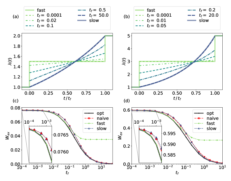
Figure 1: Form and performance of numerically produced optimal protocols for quartic trap with variable stiffness $U_{\lambda}(x)=\lambda\,x^{4}/4$ with $\lambda_{i}=1,\lambda_{f}=2$ on the left column, and $\lambda_{i}=1,\lambda_{f}=5$. on the right column. (a, b) illustrate optimal protocols for the trap stiffness, across various finite protocol duration values $t_{f}$. We see that for short times $t_{f}\ll 1$, the optimal protocol asymptotes to the fast protocol as given in Blaber et al. (2021), whereas for long times $t_{f}\gg 1$, the optimal protocol asymptotes to the slow protocol as given in Sivak and Crooks (2012). We observe discontinuous jumps at $t=0$ and $t=t_{f}$ in our numerically calculated optimal protocols, which is often the case for optimal protocols Schmiedl and Seifert (2007); Aurell et al. (2012); Blaber and Sivak (2020). (c) and (d) compare the protocol performance $W_{\mathrm{ex}}$ among the numerically calculated optimal protocol, the fast protocol, the slow protocol, and the naive protocol. We see that the optimal protocol outperforms all other protocols, with the fast and slow protocols asymptoting in performance to the optimal protocol in their respective small- and large-$t_{f}$ limits. The form and performance of these optimal protocols are qualitatively similar to those for the harmonic oscillator control case Schmiedl and Seifert (2007), which are illustrated in Supplementary Materials Fig. SM. LABEL:fig:HO.

The harmonic potential problem is exceptional in that we can solve for its optimal protocol analytically. For the vast majority of time-varying potentials, the differential Eqs. (17) with constraint (20) do not admit analytic solutions, but can be solved numerically. In this section, we briefly sketch our numerical scheme to solve Eqs. (17) and (18), and we demonstrate our approach for two classes of quartic potential problems that do not admit analytic solutions: changing the stiffness of a quartic trap, and applying a linear bias to a double-well potential.

We compare the form and performance of these optimal protocols to three other protocols: naive, fast, and slow. The naive protocol interpolates the starting and ending parameters linearly in time $\lambda(t)=\lambda_{i}+(t/t_{f})(\lambda_{f}-\lambda_{i})$, and generally is not optimal in any regime. The fast protocol, also known as the short-time efficient protocol (STEP) as developed in Blaber et al. (2021), is optimal for small-$t_{f}$ limit, and involves a step to an intermediate value $\lambda^{\mathrm{STEP}}$ for the duration of the protocol. The slow protocol first derived in Sivak and Crooks (2012), also known as the near-equilibrium protocol, is optimal for large $t_{f}$, and is obtained by considering the thermodynamic geometry of protocol parameter space induced by the friction tensor $\xi(\lambda)$, from the linear response of excess work from changes in $\lambda(t)$. With this induced thermodynamic geometry, the slow protocol is a geodesic of $\xi$ given by $\dot{\lambda}(t)\propto\xi(\lambda(t))^{-1/2}$, with $\lambda(0)=\lambda_{i}$ and $\lambda(t_{f})=\lambda_{f}$. In the Supplementary Materials Sections SM. LABEL:sec:slow-protocol and SM. LABEL:sec:fast-protocol review the slow and fast protocols in further detail, and show how we numerically produce them for our numerical study.

Here we briefly describe our discretization and integration scheme. Our lattice-discretization of space and time and approximated Fokker-Planck dynamics largely follow Holubec et al. (2019). Just as taking the continuous limit from a discrete-state master equation yields Fokker-Planck dynamics, by discretizing our configuration space onto a lattice, Fokker-Planck dynamics can be approximated by a master equation over lattice states Zwanzig (2001). Here, we approximate the configuration space by a grid of $d$ points with spacing $\Delta x$ and reflecting boundaries at $x_{\mathrm{b}}=\pm(d-1)\Delta x/2$, akin to the time-dependent Fokker-Planck discretization described in Holubec et al. (2019). Our optimal control Eqs. (17) and (18) become the ordinary differential Eqs. (9) and (10), coupled by (11). Time is discretized to $N$ time steps, with either constant or variable timesteps.

Because the transition rate matrix ${\cal{L}}_{\lambda}$ has non-positive eigenvalues Risken (1996); Wadia et al. (2022), it is numerically unstable to integrate ${\bm{\pi}}$ forward in time, as any amount of numerical noise becomes exponentially amplified. Rather, we adopt a Forward-Backward sweep method McAsey et al. (2012); Lenhart and Workman (2007), where approximate solutions for ${\bm{\rho}}^{(k)}(t)$ and ${\bm{\pi}}^{(k)}(t)$ are updated iteratively through first obtaining ${\bm{\rho}}^{(k+1)}$ by solving (9) and (11) forwards in time starting with ${\bm{\rho}}(0)={\bm{\rho}}_{i,\mathrm{eq}}$, keeping ${\bm{\pi}}(t)={\bm{\pi}}^{(k)}(t)$ fixed; and then obtaining ${\bm{\pi}}^{(k+1)}$ by solving (10) and (11) backwards in time starting with ${\bm{\pi}}(t_{f})=\bm{0}$, keeping ${\bm{\rho}}(t)={\bm{\rho}}^{(k+1)}(t)$ fixed. These forward and backward sweeps are iterated until numerical convergence of ${\bm{\rho}}^{*}(t),{\bm{\pi}}^{*}(t)$, which then is passed to $\eqref{eq:constraint-discrete}$ to obtain the optimal protocol $\lambda^{*}(t)$. More exact details of our numerical scheme may be found in Supplementary Materials Section SM. LABEL:sec:numerical-SM-description.

To measure the performance of each protocol $\lambda(t)$, we consider the excess work $W_{\mathrm{ex}}[\lambda(t)]=W[\lambda(t)]-\Delta F$, where $\Delta F=\log(Z_{f})-\log(Z_{i})$ is the free energy difference between initial and final equilibrium states, with $Z_{\lambda}=\int dx\exp(-U_{\lambda}(x))$ being the partition function. By the Second Law of Thermodynamics, $W_{\mathrm{ex}}>0$, and approaches $0$ in the quasistatic $t_{f}\rightarrow\infty$ limit. Supplementary Materials Section SM. LABEL:sec:numerical-Wex-performance specifies how we numerically compute $W_{\mathrm{ex}}$ for a given protocol.

Now we present our results for the variable-stiffness quartic trap and linearly biased double-well examples.

V.1 Quartic trap with variable stiffness

First, we consider the quartic analog of the variable stiffness harmonic oscillator, with the potential given as

$$U_{\lambda}(x)=\lambda\frac{x^{4}}{4}.$$ (28)

Figs. 1(a) and 1(b) illustrate the numerically obtained optimal protocols for variable values of protocol time $t_{f}$, for $\lambda_{i}=1,\lambda_{f}=2$; and $\lambda_{i}=1,\lambda_{f}=5$ respectively. We see that the optimal protocols for the variable stiffness quartic trap problem are qualitatively similar to the optimal protocols for the variable stiffness harmonic trap in Section 4 (derived and illustrated in Schmiedl and Seifert (2007)). For both problems, optimal protocols are continuous and monotonic with positive curvature for times $t\in(0,t_{f})$, and have discontinuous jumps at $t=0$ and $t=t_{f}$. Also plotted are the fast Blaber et al. (2021) and slow Sivak and Crooks (2012) protocols, which have been derived to be optimal for the small- and large-$t_{f}$ limits, respectively. We see that the numerically solved optimal protocol asymptotes to these protocols in the respective $t_{f}$ limits.

Figs. 1(c) and 1(d) illustrate the excess work $W_{\mathrm{ex}}$ of various protocols across different time-scales $t_{f}$. We see that the optimal protocol outperforms all three of the naive, fast, and slow protocols. The performance of the fast protocol converges to the optimal protocol performance for short time-scales $t_{f}\ll 1$. Likewise, the performance of the slow protocol converges to the optimal protocol performance for long time-scales $t_{f}\gg 1$. This is expected, and is consistent with how the optimal protocol asymptotes to the fast and slow protocols in the respective time-scales.

V.2 Linearly biased double-well

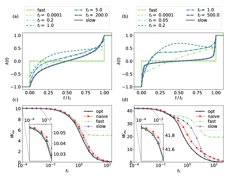
Figure 2: Numerically solved optimal protocols for the linearly biased double-well potential $U_{\lambda}(x)=E_{0}((x^{2}-1)^{2}/4-\lambda x)$, $\lambda_{i}=-1$ and $\lambda_{f}=1$; with $E_{0}=4$ in the left column, $E_{0}=16$ in the right. (a, b) illustrate the optimal protocols for the linear bias value, across various finite protocol duration values $t_{f}$. As with the quartic case in Fig. 1, here for short times $t_{f}\ll 1$ and long times $t_{f}\gg 1$, the optimal protocol asymptotes to the fast and slow protocols respectively. Unlike the slow and fast protocols, for intermediate values of $t_{f}$ the optimal protocols are not symmetric in $(t,\lambda)\rightarrow(-t,-\lambda)$. For $E_{0}=16$, we observe surprising non-monotonic protocols for $t_{f}\sim 0.2$. (c, d) depict the protocol performance $W_{\mathrm{ex}}$ between the numerically calculated optimal protocol and other protocols. Like in the quartic case, we see that the optimal protocol outperforms all other protocols, with the fast and slow protocols asymptoting in performance to the optimal protocol in their respective small- and large-$t_{f}$ limits. For $E_{0}=16$, the optimal protocol vastly outperforms the other protocols for $t_{f}\sim 2$.

Here we consider the double-well potential with wells at $x=\pm 1$ with an external linear bias

$$U_{\lambda}(x)=E_{0}\frac{(x^{2}-1)^{2}}{4}-\lambda E_{0}x.$$ (29)

Here, $E_{0}$ sets the energy scale of the ground and external potentials, with a barrier height of $E_{0}/4$ between the two wells at $\lambda=0$. This potential is commonly used in the study of bit erasure Proesmans et al. (2020); Zulkowski and DeWeese (2014), but here we allow only limited control in the form of a linear bias. We note that this problem is qualitatively similar to the Sivak and Crooks (2016), where a harmonic pulling potential with variable center is applied to a potential with two local minima separated by a barrier. We consider $\lambda_{i}=-1$ and $\lambda_{f}=1$, while varying $E_{0}$ and $t_{f}$. Setting the parameter value $\lambda=-1$ biases the potential to the left well, which sufficiently raises the right well above the barrier height and shifts the left well minimum from $x_{\mathrm{well}}=-1$ to $-1.32472$. Setting $\lambda=1$ gives a symmetric bias to the right well.

Figs. 2(a) and 2(b) illustrate optimal protocols for $E_{0}=4$ and $E_{0}=16$, which correspond to inter-well barrier heights of $1\,k_{\mathrm{B}}T$ and $4\,k_{\mathrm{B}}T$ respectively. Just as before, the optimal protocol asymptotes to the fast and slow protocols in the small- and large-$t_{f}$ limits. We note here that the optimal protocols obtained for various values of $E_{0}$ and $t_{f}$ have intriguing properties. First of all, both the fast and slow protocols are symmetric under inversion $(\lambda(t),t)\rightarrow(-\lambda(t),t_{f}-t)$, which arises from the symmetry $U_{\lambda}(x)=U_{-\lambda}(-x)$ with $\lambda_{f}=-\lambda_{i}$, and the construction of these protocols. We see though that the optimal protocol obtained by solving (17) and (18) do not follow this this symmetry for intermediate values of timescale $t_{f}$. This discovery of barrier crossing optimal protocols breaking symmetry was first made in Engel et al. (2022). At first this symmetry-breaking may seem counter-intuitive, but this can be understood by noting that $\lambda_{i}$ and $\lambda_{f}$ play completely different roles in our optimal control problem: $\lambda_{i}$ specifies the initial condition $\rho(x,0)$, while $\lambda_{f}$ specifies $U_{f}(x)$ in the cost function.

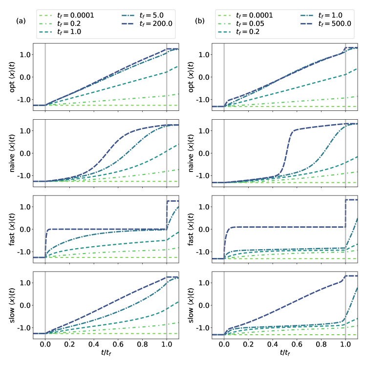
Figure 3: The evolution of the mean position $\langle x\rangle(t)$ for the linearly biased double-well problem $U_{\lambda}(x)=E_{0}((x^{2}-1)^{2}/4-\lambda x)$, across various protocol duration values $t_{f}$. Here, $\lambda_{i}=-1$ and $\lambda_{f}=1$, with (a) $E_{0}=4$, and (b) $E_{0}=16$. The first row depicts the optimal protocol, the second the naive protocol, the third the fast protocol, and the fourth the slow protocol. For the optimal protocol, $\langle x\rangle(t)$ increases monotonically with near-constant velocity, which we argue is a generic property of limited-control optimal controls. In comparison, the naive, fast, and slow protocols evolve the mean $\langle x\rangle(t)$ with much more variable velocity. The deviation from constant-velocity roughly corresponds to larger $W_{\mathrm{ex}}$ values, as depicted in Figs. 2(c) and 2(d).

Furthermore, not only do we find non-symmetric protocols, we discover that for $E_{0}=16$, the optimal protocol $\lambda(t)$ is non monotonic at certain intermediate timescales $t_{f}\sim 0.2$. This result is surprising, given that the underlying stochastic system (12) is overdamped — it has no momentum degrees of freedom that could incentivize overshoots. To our knowledge, no optimal or approximately-optimal protocols for a single parameter $\lambda$ have been reported to exhibit this sort of non-monotonic behavior. In this regime, the optimal protocol cannot be interpreted as a geodesic for an underlying thermodynamic metric, as the latter can only produce monotonic protocols.

To explain this overshoot, we consider the mean position of the probability density under the optimal protocol $\langle x\rangle=\int\rho(x,t)\,x\,dx$ as a function time $t$. This is shown in Figs. 3(a) and 3(b), where we see $\langle x\rangle$ increases at a nearly constant rate under the optimal protocol. This may be interpreted as the limited-control optimal protocol allowing barrier-crossing to occur at an approximately constant velocity. In Supplementary Materials Section SM.LABEL:sec:opt-transport, we draw from optimal transport theory to show that when full control over the potential is allowed, $\langle x\rangle$ always maintains a constant speed throughout the optimal trajectory. This suggests that insofar as a limited-control optimal protocol should approximate the full-control optimal protocol, it drives the mean of the probability distribution to travel with near-constant velocity, even if requiring an overshoot as is the case for the $E_{0}\sim 16,t_{f}\sim 0.2$ regime.

Figs. 2(c) and 2(d) illustrate the performance of these protocols. Just as we found for the harmonic potential, the OCT protocol outperforms all three other considered protocols, with performance of fast and slow protocols approaching the optimal protocol performance in their respective $t_{f}$ limits. We see that for barrier height $E_{0}=16$, the optimal protocol vastly outperforms all other protocols at intermediate $t_{f}$ values. For instance, at $t_{f}=2$ the optimal protocol gives $W_{\mathrm{ex}}=10.61$, which is significantly smaller than the naive protocol $W_{\mathrm{ex}}=16.12$ and slow protocol $W_{\mathrm{ex}}=26.77$ values. This shows the existence of truly far from equilibrium regimes, for which protocols derived assuming either fast or near-equilibrium approximations deviate significantly from the true, fully non-equilibrium optimal protocol, in both form and performance.

VI Discussion

It is typically the case in experimental and engineering contexts that only a finite set of degrees of freedom of a system is controllable. We have shown that the problem of finding work-minimizing optimal protocols is naturally framable as an optimal control theory (OCT) problem. Using tools and techniques from OCT, we have devised a method to derive optimal protocols in the case where there is only limited control of the form of the system’s potential. Our framework allows us to reproduce known analytic results for the control of a harmonic oscillator, as well as to efficiently calculate optimal protocols numerically for a large class of limited-control potentials.

Previous work on dissipation-minimizing optimal protocols revealed thermodynamic geometry on protocol parameter space through the friction tensor Sivak and Crooks (2012); Wadia et al. (2022), and on probability density space through the $L^{2}$-Wasserstein metric Watanabe and Minami (2022); Dechant and Sakurai (2019); Nakazato and Ito (2021); Chen et al. (2019). We have found that the protocol optimization problem has a deep Hamiltonian structure, typical of OCT problems Liberzon (2011). It is interesting to ponder what insights may be gleaned from the study of optimal protocols for non-equilibrium processes when both Riemmanian and symplectic structures are considered together.

It is straightforward to generalize our results configuration and parameter spaces that are multi-dimensional, which suggests a number of natural extensions. First, by allowing time-varying control of temperature $\beta^{-1}=k_{\mathrm{B}}T$ and asserting time-periodicity for the protocol, we can construct optimal finite-time heat engines arbitrarily far from equilibrium, building off of Frim and DeWeese (2021a); Watanabe and Minami (2022); Ye et al. (2022). Cyclical protocols may also be considered for when the state space and/or configuration space are non-Euclidean manifolds Frim et al. (2021); e.g., for the external control of rotory motor proteins like $F_{o}F_{1}$ Lucero et al. (2019). Finally, it would be intriguing to extend our framework to the study of underdamped systems where both position and velocity degrees of freedom $(x,v)$ make up the configuration space Gomez-Marin et al. (2008); Muratore-Ginanneschi (2014), as because the kinetic term of the underlying Klein-Kramers equation cannot be controlled, control is intrinsically limited to just the spatial degrees of freedom.

When the configuration space has many degrees of freedom, the curse of dimensionality kicks in, where the memory required to store the probability distribution is exponential in the number of dimensions of the configuration space Kappen (2005). In this case, it may be more computationally tractable to sample individual stochastic trajectories to compute the friction tensor Sivak and Crooks (2012); Rotskoff and Crooks (2015) or gradients of the protocol Engel et al. (2022) in order to calculate optimal protocols. It will be of interest to study the effectiveness of configuration space dimensionality reduction techniques (e.g., density functional theory te Vrugt et al. (2020), Zwanzig-Mori projection operators Zwanzig (2001)) to make the calculation of optimal protocols through our framework computationally tractable for high dimensional configuration spaces.

We have shown that optimal control theory is a natural and powerful framework for the design and study of thermodynamically optimal protocols. In the spirit of Roach et al. (2018), it is our hope that through considering the optimal control of non-equilibrium probability densities considered here and elsewhere Annunziato and Borzì (2013); Palmer and Milutinović (2011); Bakshi and Theodorou (2020), we may better understand how it is that biological systems, which operate far from equilibrium, function efficiently across vastly different length- and time-scales.