A Framework for Checkpointing and Recovery of Hierarchical Cyber-Physical Systems

Abstract.

This paper tackles the problem of making complex resource-constrained cyber-physical systems (CPS) resilient to sensor anomalies. In particular, we present a framework for checkpointing and roll-forward recovery of state-estimates in nonlinear, hierarchical CPS with anomalous sensor data. We introduce three checkpointing paradigms for ensuring different levels of checkpointing consistency across the hierarchy. Our framework has algorithms implementing the consistent paradigm to perform accurate recovery in a time-efficient manner while managing the tradeoff with system resources and handling the interplay between diverse anomaly detection systems across the hierarchy. Further in this work, we detail bounds on the recovered state-estimate error, maximum tolerable anomaly duration and the accuracy-resource gap that results from the aforementioned tradeoff. We explore use-cases for our framework and evaluate it on a case study of a simulated ground robot to show that it scales to multiple hierarchies and performs better than an extended Kalman filter (EKF) that does not incorporate a checkpointing procedure during sensor anomalies. We conclude the work with a discussion on extending the proposed framework to distributed systems.

1. Introduction and Related Work

With the advent of cyber-physical systems (CPS) in critical day-to-day tasks from self-driving automobiles to medical devices, there is a heightened urgency to build systems resilient to sensor anomalies. Sensors are a vital part of CPS that are easily susceptible to anomalies that can arise from hardware and software faults (Sharma et al., 2010), (Ni et al., 2009), changes in the physical environment around a sensor (Park et al., 2015), (Petit et al., 2015), (Guo et al., 2018) or malicious attackers (Mo and Sinopoli, 2010), (Rutkin, 2013). Some examples of faults include calibration issues (Sharma et al., 2010) and lost messages (Ni et al., 2009). Examples of non-invasive anomalies from environment changes involve GPS obfuscation in tunnels (Park et al., 2015), obscured video cameras and lidars in adverse weather conditions (Petit et al., 2015), interference between sensors such as infrared and lidar (Guo et al., 2018), etc. A couple of examples of malicious attacks are false-data injection attacks (Mo and Sinopoli, 2010) and GPS spoofing (Rutkin, 2013). Ensuring the continued safe functioning of CPS under various kinds of sensor anomalies, however, is a challenging research problem.

Different solutions have been proposed for sensor anomaly resiliency of CPS (Guo et al., 2018), (van Wyk et al., 2019), (Bu et al., 2017), (Mo and Sinopoli, 2010), (Park et al., 2015), (Pajic et al., 2014) (Shoukry et al., 2017), (Miao et al., 2013). Diverse anomaly detection systems (ADS) have been explored (Guo et al., 2018), (van Wyk et al., 2019), (Bu et al., 2017), (Mo and Sinopoli, 2010), (Park et al., 2015). Some ADS have been proposed for sensor anomaly detection (van Wyk et al., 2019), (Bu et al., 2017), (Mo and Sinopoli, 2010), (Park et al., 2015) whereas others are instrumental in finding actuator anomalies (Guo et al., 2018). Building upon various ADS’, resilient state estimators (RSE) (Pajic et al., 2014) which solve a constrained minimization problem between sensor measurements and state evolution have been proposed. Other control methods resilient to anomalies based on SMT (Satisfiability Modulo Theory) (Shoukry et al., 2017) and game theory (Miao et al., 2013) have also been delved into.

These methods are computationally intensive and don’t account for hardware limitations. In practice, these algorithms will have to be implemented in platforms like embedded computers and micro-controllers with limited computational resources and system memory. On the other hand, vanilla state-estimation with Kalman Filters is not computationally taxing but also isn’t resilient to sensor anomalies. To find a middle ground, cyber-physical checkpointing and roll-forward recovery was introduced in (Kong et al., 2018).

Checkpointing and roll-forward recovery (RFR) (Kong et al., 2018) can be used in case of detected sensor anomalies (and hence incorrect state-estimates) in order to recover state-estimates from a periodically securely saved correct value (called a checkpoint). Between consecutive checkpoints, control inputs applied to actuators are also saved in secure memory. Recovery takes place by using these saved control inputs and ”rolling” the system states forward from the checkpoint to the current time. Then, using the recovered state-estimate, we can generate a sensor anomaly resilient control command.

It makes use of sensor ADS and can incorporate aspects of the RSE (Pajic et al., 2014) and other sensor anomaly resilient control methods (Shoukry et al., 2017), (Miao et al., 2013) in the roll-forward procedure. This means that checkpointing and RFR can also be applied over existing resiliency methods as an extra layer of defense.

In (Kong et al., 2018), checkpointing and RFR is shown to be better than a Kalman Filter in prediction of state-estimate for linear time invariant (LTI) systems under sensor anomalies.

Moreover, checkpointing and RFR can manage the tradeoff between system resources (memory and compute time) and accuracy of recovered state-estimate by not having to save every state-estimate, control input while also utilizing a shorter iterative ”rolling” forward procedure. This in turn allows for its application to resource-constrained hardware.

Although a good first step, (Kong et al., 2018) does not address checkpointing and recovery for complex CPS with hierarchical distributed control architectures and nonlinear dynamics even though most CPS today, such as self-driving cars and diabetic implants, fall into that category (Rajamani, 2011), (et al., 2011). There are two important challenges associated with checkpointing and RFR for nonlinear, hierarchical systems. (1) Hierarchical systems necessitate algorithms to snapshot and locate consistent checkpoints with coordination between sub-systems. (2) With increased complexity from non-linearities and the hierarchy, we need to direct attention to preserving the accuracy of recovered state-estimates while managing the tradeoff with system resources, coordinating amongst sub-systems with diverse ADS outputs and ensuring timely-communication between sub-systems with a time-efficient roll-forward strategy.

We tackle the first challenge by introducing three checkpointing paradigms for checkpointing with different levels of consistency. We detail a coordinating algorithm scalable to multiple hierarchies, each operating at different frequencies.

We address the second challenge with an analysis of the tradeoff between accuracy and system resources and demonstrate the ability to manage this tradeoff by tuning checkpointing frequency. We propose a RFR algorithm that performs time-efficient recovery with minimal checkpoint usage while allowing for the interplay between sub-systems with different ADS (specific or generic). We also discuss resolutions for the issues of communication security and minimal lag in extending our framework to distributed systems.

Further, there is a need to guarantee bounds on the difference between recovered state-estimate and ground truth (a.k.a. recovered state-estimate error) and quantify the maximum permissible duration of application of the above algorithms. Additionally, investigating the tradeoff between system resources and accuracy leads to questions about the accuracy-resource gap (which is the difference between an accuracy-optimal state-estimate recovered with most-frequent checkpointing and one from some arbitrary checkpointing frequency).

In this paper, under assumptions on bounded noise, jacobian and certain non-linearity, we guarantee bounds on recovered state-estimate error regardless of linear or nonlinear dynamics. We analyze its variation under different checkpointing frequencies which in turn leads to an analysis in tradeoffs between accuracy and system resources and bounds on the accuracy-resource gap. Also, given maximum admissible error, we present a bound on the maximum tolerable duration of anomalies in sensor data.

We evaluate the proposed framework on a case-study of a simulated ground robot with one outer loop and two inner loops. The case study demonstrates scalability of the framework to multiple hierarchies and that the proposed framework lowers estimation error (when given anomalous sensor data) significantly when compared to an extended Kalman filter estimator in every loop.

In summary, this paper makes the following contributions.

• A framework for checkpointing and roll-forward recovery (RFR) of nonlinear, hierarchical systems (Section 4)

• A theoretical analysis of bound on recovered state-estimate error, maximum tolerable anomaly duration and tradeoff between checkpointing frequency, accuracy and system resources. (Section 5)

• A numerical validation on a simulated ground robot that demonstrates scalability and efficacy. (Section 6)

2. Background and Preliminaries

In this section, we mention the background information on cyber and physical checkpointing and recovery.

2.1. Cyber state checkpointing and rollback recovery

Cyber checkpointing and rollback recovery (Manabe, 2001) is an important fault-tolerance technique for long-running applications on distributed computing systems (e.g. distributed optimization). It lets the application restart from the last saved snapshot (or checkpoint) of its state rather than restarting from the beginning.

Cyber state recovery takes place by rolling-back to a checkpoint and restarting a task. Consistent checkpoints are preferred as they prevent the domino effect (i.e. multiple rollbacks to find a state with sufficient information to restart the task) (Manabe, 2001). A consistent cyber state checkpoint is a periodically saved consistent cyber state.

Definition 2.1.

A consistent cyber state is a cyber state in which no message is recorded as received in one process and as not yet sent in another process (Manabe, 2001).

Figure 1 shows examples of consistent and inconsistent cyber checkpoints. Note that a cyber state with all elements saved at the same time is consistent since it satisfies Definition 2.1.

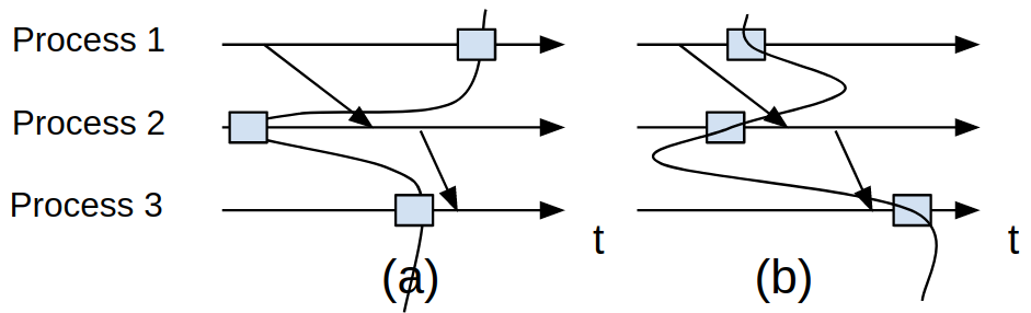
Figure 1. (a) Consistent & (b) inconsistent cyber checkpoint

2.2. Physical state-estimate checkpointing and roll-forward recovery (RFR)

In (Kong et al., 2018), the following simple linear time invariant (LTI) system is considered

(1) $$x_{k+1} =Ax_{k}+Bu_{k}+w_{k}$$

(2) $$y_{k} =Cx_{k}+v_{k}$$

where $x_{k}\in\mathbb{R}^{n}$, $u_{k}\in\mathbb{R}^{m}$, $y_{k}\in\mathbb{R}^{p}$, $w_{k}\sim\mathcal{N}(0,Q)$ and $v_{k}\sim\mathcal{N}(0,R)$. State-estimates (denoted $\hat{x}_{k}$) are produced by a Kalman Filter.

The concept of checkpointing and physical state recovery for the simple LTI system (1), (2) was introduced in (Kong et al., 2018). Physical state-estimate recovery occurs by rolling state-estimate elements forward to current time from a consistent checkpoint. Checkpoints are values of state-estimate saved periodically in stable secure memory.

Definition 2.2.

Consistent physical state-estimate of a LTI system such as the one in (1), (2) is a physical state-estimate which has all of its elements’ values from the same time-instant (Kong et al., 2018).

Figure 2 shows examples of consistent and inconsistent physical state-estimate checkpoints for LTI system via boxes with curved line passing through. These boxes represent values at or just before checkpointing time that are saved as the checkpoint. Note that the notion of ”the same time” can be modified to allow a bounded precision between clocks used to timestamp local states. For simplicity, this paper assumes the existence of globally consistent time (Kopetz, 2011).

Figure 2. (a) Consistent and (b) inconsistent physical state-estimate checkpoints for a LTI system.

Next, the algorithm in (Kong et al., 2018) assumes a specific ADS that tells the controller (at time $k$) that the first $q$ elements of the state-estimate have been affected. These affected elements are denoted $\hat{x}_{k,(1,q)}$ and healthy elements are denoted $\hat{x}_{k,(q+1,n)}$.

When $q$ is at least one, RFR takes place. Physical state-estimate (at time $k$) is recovered from a checkpoint of state-estimate that was created $N$ time steps behind current time (denoted $\bar{x}_{k-N}$), using control inputs saved between the checkpoint time and current time, with repeated use of the Kalman Filter’s predict step ($x_{k+1}=Ax_{k}+Bu_{k}$) as follows,

(3) $$\hat{x}^{R}_{k} =A^{N}\bar{x}_{k-N}+\sum_{i=1}^{N}A^{i-1}Bu_{k-i}.$$

Then, the $q$ affected elements of state-estimate are updated with roll-forward recovered value as follows,

(4) $$\hat{x}_{k,(1,q)} =\hat{x}^{R}_{k,(1,q)}.$$

Lastly, this updated state estimate is used to generate control inputs that are sent to an actuator. We reiterate that this work on checkpointing and recovery in (Kong et al., 2018) is limited in application to a simple LTI system with an assumed specific ADS.

We present a more general problem with a nonlinear hierarchical system that consist of 2 feedback control loops (a.k.a. sub-systems) in the following section. Each of the sub-systems may have a specific or generic ADS (Section 3.5). Our framework, introduced in Section 4, is applicable to this generalized problem and can be extended to distributed systems under conditions discussed in Section 7.

3. Problem Formulation

In this section we present the hierarchical system model and measurement model, anomaly model, estimator, controllers, anomaly detection systems, cyber-physical system model and objective.

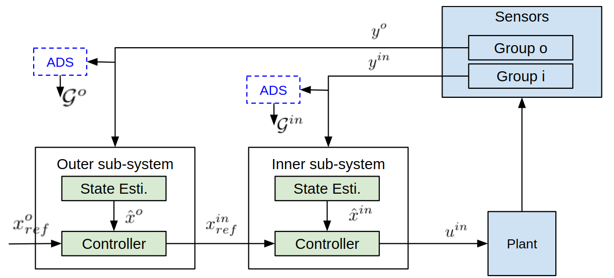
Figure 3. Block diagram of the hierarchical system

3.1. Physical System and Measurement Model

We assume that the physical system is a collection of the inner and outer sub-systems (or loops) as shown in Figure 3 and represented with superscript $j\in\{in,o\}$. We have discrete-time nonlinear sub-system dynamics and measurement models as follows

(5) $$x^{j}_{k+1} =f^{j}(x^{j}_{k},u^{j}_{k})+\omega^{j}_{k},\;\;\;\;x^{j}_{0}\sim\mathcal{N}(\mu^{j}_{0},\Sigma^{j}),\;\;\;\omega^{j}_{k}\sim\mathcal{N}(0,Q^{j})$$

(6) $$y^{j}_{k} =g^{j}(x^{j}_{k},u^{j}_{k})+\gamma^{j}_{k},\;\;\;\;\;\gamma^{j}_{k}\sim\mathcal{N}(0,R^{j})$$

where $x^{j}_{k}\in\mathbb{R}^{n_{x}^{j}}$, $y^{j}_{k}\in\mathbb{R}^{n_{y}^{j}}$ and $u^{j}_{k}\in\mathbb{R}^{n_{u}^{o}j}$ are the physical state vector, measurement vector and control input (at time $k$) of the $j$th sub-system. We have process and measurement covariance matrices $Q^{j},R^{j}$ for the $j$th subsystem.

3.2. State Estimation

In each of the $(in)$ and $(o)$ sub-systems, we assume an estimator that calculates state-estimate with a predict step and improves it with an update step. Some examples are the RSE (Pajic et al., 2014) & the extended Kalman filter (EKF) which can be represented, in the $j$th sub-system, with a predict step (7), gain calculation (7) & update step (8),

(7) $$\hat{x}^{j}_{k+1|k} =\text{predict}^{j}(\hat{x}_{k}^{j},u_{k}^{j})\;\;\;\;\;K^{j}_{k}=\text{gain}^{j}(\hat{x}_{k}^{j},Q^{j},R^{j})$$

(8) $$\hat{x}^{j}_{k+1} =\text{update}^{j}(\hat{x}^{j}_{k+1|k},K^{j}_{k},{y^{j}_{k}}^{\prime})$$

3.3. Controllers

3.3.1. Reference Trajectory

We assume that reference trajectory’s state (at time $k$) denoted $x^{o}_{k,ref}$ is provided to the outer loop. The outer loop generates control $u^{o}_{k}$ which is transformed by map $T:\mathbb{R}^{n^{o}_{u}}\to\mathbb{R}^{n^{in}_{x}}$ to obtain inner loop reference value $x^{in}_{k,ref}=T(u^{o}_{k})$.

3.3.2. Control

We assume that each loop uses a controller abstracted as $u^{j}_{k}=h^{j}(\hat{x}^{j}_{k},x^{j}_{k,ref}),\;\;\;j\in\{in,o\}$. We also assume that each loop $j$ runs at a frequency $\mu^{j}$. Some examples of controllers that can be used are PID (Kong et al., 2018), neural network (Ivanov et al., 2019), dynamic inversion (cle, 2013), model predictive (Kong et al., 2015) controllers, etc.

3.4. Anomaly Model

We assume that sensor anomalies lead to change in the readings of a subset of sensors (represented as $\mathcal{S}^{a}$), which results in the following generalized model:

(9) $${y^{j}_{k}}^{\prime}=g^{j}({x^{j}_{k}}^{\prime},u^{j}_{k})+\gamma^{j}_{k}+\Gamma^{j}y^{j,a}_{k},\;\;\;j=in,o$$

where $y^{j,a}_{k}\in\mathbb{R}^{n_{y}^{j}}$ is the anomalous addition (at time $k$) to the sensor readings of the $j$th sub-system. We also have sensor selection matrices $\Gamma^{j}=diag(\eta^{j}_{1},...,\eta^{j}_{n_{y}^{j}})$ where $\eta^{j}_{i}=1$ if $i$th sensor of sub-system $j$ is in $\mathcal{S}^{a}$. This results in anomalous measurement vectors ${y^{j}_{k}}^{\prime}\in\mathbb{R}^{n_{y}^{j}}$ and affected states ${x^{j}_{k}}^{\prime}\in\mathbb{R}^{n_{x}^{j}}$ (differs by ^′ from healthy values). As difficulty in recovering accurate state-estimates increases with anomaly duration, we primarily concern ourselves with transient/intermittent anomalies such as GPS signal loss in tunnels (Park et al., 2015), lidar affected by reflective surfaces, fog or infrared light (Petit et al., 2015), cameras impaired by harsh lights or rain (Guo et al., 2018), etc..

3.5. Anomaly Detection System (ADS)

Most ADS fall into two broad categories - a specific detector and a generic detector. The specific detector (e.g. deep neural network detector (van Wyk et al., 2019), $\chi^{2}$ detector (Mo and Sinopoli, 2010), sensor-fusion detector (Park et al., 2015)) provides a list of sensors with anomalies whereas the generic detector (e.g. fuzzy logic detector (Bu et al., 2017)) can only inform the system about the presence of some anomalous data without specifying which sensors have anomalies. We assume an ADS in each sub-system of the hierarchy and abstract an ADS of sub-system $j$ as,

(10) $$\mathcal{G}^{j}_{k} =f_{ADS}({y^{j}_{k}}^{\prime},...,{y^{j}_{k-\mathcal{T}^{j}+1}}^{\prime},k)$$

where the detection function $f_{ADS}:\mathbb{R}^{\mathcal{T}^{j}(n_{y}^{j})}\to\{0,1\}^{m}$ takes as input a window of measurements of size $\mathcal{T}^{j}$ (detection time for sub-system $j$) and current time-instant $k$. It outputs either a Boolean vector $\mathcal{G}^{j}_{k}\in\{0,1\}^{n_{y}^{j}}$ whose $i$th element takes a value of 1 when the $i$th sensor has anomalous data (for a specific detector) or a simple Boolean $\mathcal{G}^{j}_{k}\in\{0,1\}$ representing the presence of some sensors with anomalous data (for a generic detector). Thus the same abstraction can be used for both specific and generic detectors and each sub-system may have either of the two.

Further, some ADS such as the sensor-fusion based detector (Park et al., 2015) require that at least some $\zeta>0$ sensors are healthy at time $k$ for detection. Others like the $\chi^{2}$ detector (Mo and Sinopoli, 2010) assume prior knowledge on sensor performance for detection. Thus, the extent of protection delivered by our framework and its performance in recovering state-estimates depends on the detection capability of the ADS.

3.6. Cyber-Physical System

The CPS is a combination of the physical elements (physical system, sensors, actuators) and software elements (state estimators, ADS, controllers) described in the previous section. The system’s physical state (denoted $x_{k,p}\in\mathbb{R}^{n_{x}^{in}+n_{x}^{o}}$) contains the physical states of each sub-system. The system’s cyber state (denoted $x_{k,c}\in\{0,1\}^{m^{in}+m^{o}}$) contains the Boolean output sent by the ADS to the sub-systems. The CPS state (denoted $x_{k,CPS}\in\mathbb{R}^{n_{x}^{in}+n_{x}^{o}}\times\{0,1\}^{m^{in}+m^{o}}$) is a combination of the system’s physical and cyber states. We have physical, cyber and CPS state as follows,

(11) $$x_{k,p} =\begin{bmatrix}x^{in}_{k}\\ x^{o}_{k}\end{bmatrix}\;\;\;x_{k,c}=\begin{bmatrix}\mathcal{G}^{in}_{k}\\ \mathcal{G}^{o}_{k}\end{bmatrix}\;\;\;x_{k,CPS}=\begin{bmatrix}x_{k,p}\\ x_{k,c}\end{bmatrix}.$$

3.7. Objective

Our primary objective is to recover CPS state-estimates at time $k$ when facing sensor anomalies using the checkpointing and RFR framework while working within the system’s hardware constraints. This includes striving for a balance between accuracy and resource utilization. Then, we use recovered state-estimates to generate sensor anomaly resilient control commands $u^{in}_{k},u^{o}_{k}$. Our secondary objective is to ensure that the recovered state-estimate error remains within acceptable bounds by halting application of proposed framework after maximum tolerable anomaly duration.

4. Framework for Checkpointing and Recovery

In this section, we propose our consistent checkpointing and RFR framework for hierarchical systems, comprised of Algorithms 1, 2, 3, that integrates into the hierarchical system as shown via components called ADS, ”recovery”, ”checkpointing” and ”coordinator” in Figure 4.

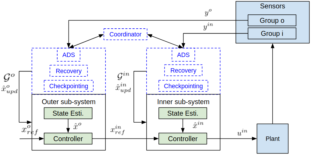
Figure 4. Block diagram of the framework and ADS (in blue) integrated into the hierarchical system

We begin this section by comparing three checkpointing paradigms and their analogous frameworks in Section 4.1. We propose using the consistent paradigm and associated consistent framework. Then, we explain the checkpointing and RFR protocols of Algorithms 1, 2 in Sections 4.2, 4.3 and the role of the coordinator (Algorithm 3) in Section 4.4.

4.1. Checkpointing Paradigms

For dealing with hierarchical systems, we extend Definition 2.2 to,

Definition 4.1.

Consistent physical state-estimate for the hierarchical CPS is a same time-instant combination of consistent physical state-estimates of every sub-system (which has all of it’s elements from the same time-instant).

An inconsistent physical state-estimate of the hierarchical CPS can be either partly or fully inconsistent (see Figure 5(b) and (c)). Partly inconsistent physical state estimates in the CPS are combinations of consistent physical state-estimates of inner and outer subsystems at different time-instants (see Figure 5(b)). Fully inconsistent physical state-estimates are combinations of inconsistent physical state-estimates of inner and outer subsystems (see Figure 5(c)). Checkpoints are physical state-estimates of the CPS saved every user-specified time-interval in stable secure memory.

Figure 5. (a) Consistent,(b) partly inconsistent & (c) fully inconsistent physical state-estimate checkpoints for hierarchical CPS. Values saved at/ just before checkpointing time.

The distinctions between the three types of checkpoints is important when considering possible alternates to the proposed framework. We define them below.

Definition 4.2.

Consistent framework: proposed framework with recovery from consistent physical state-estimate checkpoints of CPS.

Definition 4.3.

Partially inconsistent framework: alternate framework where physical state-estimate checkpoints consistent in each sub-system but not in the hierarchy are used for recovery.

Definition 4.4.

Inconsistent framework: alternate framework where fully inconsistent physical state-estimate checkpoints of CPS are used for recovery.

These three frameworks are shown in Figure 6 (a), (b) & (c), where all elements of outer and inner state estimates have been detected as anomalous at times $k_{1}+2\text{dt}^{o}$ and $k_{2}+3\text{dt}^{in}$ because of sensor anomalies that started at $k_{1}+\text{dt}^{o}$ and $k_{2}+\text{dt}^{in}$ respectively.

Figure 6. (a) Proposed consistent framework and alternates- (b) partially inconsistent, (c) fully inconsistent frameworks when anomalous sensor data starts with red shaded region and is detected at values with red cross marks. RFR (green arrows) uses latest checkpoint before start of the anomaly.

In framework (a), we have RFR from consistent checkpoints at $k_{1}$ (for the outer loop) and $k_{2}$ (for the inner loop) depicted by curved green arrows.

In framework (b), sub-system $(o)$ with checkpoint at $k_{1}$ can recover from said checkpoint. On the other hand, sub-system $(in)$ cannot recover from its failed checkpoint at $k_{2}+2\text{dt}^{in}$. Instead, the recovery (depicted by right-angled green arrow) has to begin from the checkpoint behind the most-recent checkpoint which is not shown in the figure. If this checkpoint is distant to the current time, we will have different roll-forward times for each sub-system. In practice, this could lead to delays in computing control inputs and undesirable (or even unstable) behaviour.

In framework (c), some elements of both subsystems $(in),(o)$ have checkpoints in the anomalous period and so we cannot have recovery from said checkpoints for those elements. Instead, for those elements, the recovery (depicted by right-angled green arrows) has to begin from the checkpoint behind the most-recent checkpoint which is again not shown in the figure. Thus, similar to (b), this could result in undesirable behaviour of the CPS.

Although all the above three frameworks can find a conceivable use in hierarchical CPS, we employ only the first consistent framework throughout this work. This is because, we see that, in the situation depicted in Figure 6, the proposed consistent framework fares better than alternate inconsistent frameworks (b) and (c). Further, identifying most-recent checkpoint outside anomaly duration for each and every sub-system in (b), and for each and every element in (c), requires increased computational resources and time as compared to the proposed framework (a).

Thus, to avoid both undesirable behaviour and additional overhead in resource utilization, we proceed with the consistent framework rather than the alternate inconsistent frameworks.

4.2. Consistent framework for the hierarchical system and its checkpointing protocol

Algorithm 1 presents the consistent checkpointing procedure and initiates the RFR when anomalous data is received in every sub-system $j$.

In Line 1, the algorithm sets the loop rate $\mu^{j}$ and initializes state-estimate $\hat{x}_{0}^{j}$. In lines 2-18, we have a loop running at the specified loop rate which terminates after a preset time-instant T or when anomaly exceeds maximum tolerable duration (Line 17). At time-instant $k$ in Line 3, Algorithm 1 begins by receiving a coordinator Boolean $c_{k}^{j}$ from the consistent checkpointing coordination protocol of Algorithm 3. If this coordinator Boolean evaluates to 1, a checkpointing procedure (Lines 13-17) may be initiated downstream. Before that, the sub-system estimates state $\hat{x}^{j}_{k}$ and receives estimator gain $K_{k}^{j}$ in Line 4 via predict, gain calculation and update steps. In Line 5, the ADS takes in a window of measurements (of length detection time $\mathcal{T}^{j}_{k}$ when $k\geq\mathcal{T}^{j}_{k}$ or else of length $k$) and gives out either a Boolean vector (for a specific detector) or a simple Boolean (for a generic detector) as previously discussed in Section 3.5. The algorithm also has access to value of detection time $\mathcal{T}^{j}_{k}$.

In Line 6, it calculates the ’anomaly detected’ Boolean as either a union of the Boolean elements of $\mathcal{G}^{j}_{k}$ for a specific detector or the simple Boolean $\mathcal{G}^{j}_{k}$ itself for a generic detector. If an anomaly was detected (i.e., the ’anomaly detected’ Boolean is ’True’), then it calls the RFR algorithm given by Algorithm 2 (Lines 7-9). Suppose an anomaly was detected, then after obtaining the recovered state-estimate, it calculates an anomaly-resilient control value in Line 10. If no anomaly was detected, a standard control value is calculated in Line 10.

Lastly, control inputs are securely saved in an array (Line 11). Further, if no anomaly was detected and the coordinator Boolean received at the start evaluates to 1, a checkpoint of cyber-physical state-estimate (i.e., physical state-estimate and ADS outputs) is appended to an array of checkpoints (Lines 12,13). The time of checkpointing is also appended to an array (Line 14). Both these arrays are securely saved in Line 15. If the current anomaly’s duration exceeds the maximum tolerable anomaly duration, then it exits to a safe stop (Line 17) or else it repeats this process.

input : sensor measurements: ${y_{k}^{j}}^{\prime}$, reference trajectory: $x^{j}_{k,ref}$, maximum tolerable anomaly duration: $\mathcal{T}^{j}_{\text{max}}$

output : anomaly-resilient control commands: $u_{k}^{j}$

1 initialize: loop rate = $\mu^{j}=\frac{1}{dt^{j}}$, $\hat{x}_{0}^{j}$

2 for k = 1 to T in time steps of $dt^{j}$ do

3       $c_{k}^{j}$ $\leftarrow$ short wait for Boolean from consistent checkpointing coordination() in coordinator

4       $\hat{x}^{j}_{k},K^{j}_{k}\leftarrow\text{update}^{j}(\text{predict}^{j}(\hat{x}^{j}_{k-1},u_{k-1}^{j}),\text{gain}^{j}(\hat{x}_{k-1}^{j},Q^{j},R^{j}),{y_{k}^{j}}^{\prime})$

5       $\mathcal{G}^{j}_{k}$, $\mathcal{T}^{j}_{k}$ $\leftarrow$ $f_{ADS}({y^{j}_{k}}^{\prime},...,{y^{j}_{k-\mathcal{T}^{j}_{k}+1}}^{\prime},k)$

6       anomaly_detected${}_{k}^{j}$ = $\begin{cases}\bigcup\limits_{i=1}^{n_{y}^{j}}\mathcal{G}^{j}_{k,i},\text{ for specific detector}\\ \mathcal{G}^{j}_{k},\text{ for generic detector}\end{cases}$

7       if anomaly_detected${}_{k}^{j}$ = True then

8             $\hat{x}^{j}_{k}$ $\leftarrow$ roll-forward recovery $\left(\hat{x}^{j}_{k},K^{j}_{k},\mathcal{G}^{j}_{k},\mathcal{T}_{k}^{j}\right)$

9       end if

10      $u_{k}^{j}$ $\leftarrow$ $h^{j}\left(\hat{x}_{k}^{j},x^{j}_{k,ref}\right)$

11       controls.append $\left(u_{k}^{j}\right)$; secure_save controls

12       if anomaly_detected${}_{k}^{j}$ = False and $c_{k}^{j}$ = True then

13             checkpoints.append $\left(\hat{x}^{j}_{k},\mathcal{G}^{j}_{k}\right)$

14             save_times.append($k$)

15             secure_save checkpoints, save_times

16       end if

17      if anomaly duration $>\mathcal{T}^{j}_{\text{max}}$ then exit to safe stop

18      

19 end for

Algorithm 1 Consistent Checkpointing, Roll-forward Recovery and Sensor-anomaly Resilient Control Framework on Sub-system $j\in\{in,o\}$

4.3. Roll-forward recovery (RFR) protocol for the hierarchical system

We explain Algorithm 2 which presents the RFR protocol in this subsection. Once a sub-system receives anomalous sensor data, Algorithm 2 is triggered and it proceeds to find the latest consistent checkpoint across all sub-systems (in Line 2) via the most-recent consistent checkpoint time protocol of Algorithm 3.

input : state-estimate $\hat{x}_{k}^{j}$, estimator gain matrix $K^{j}_{k}$, ADS Boolean(s) $\mathcal{G}^{j}_{k}$ and detection time $\mathcal{T}_{k}^{j}$

output : recovered / updated state-estimate $\hat{x}_{k}^{j}$

1

2secure_retrieve: checkpoints, save_times, controls

3 $k_{1}$ $\leftarrow$ most-recent consistent checkpoint time from coordinator($\mathcal{T}_{k}^{in}$, $\mathcal{T}_{k}^{o}$)

4 if anomaly_detected${}_{k-1}^{j}$ = False then

5       $\hat{x}^{j,R}_{k}\leftarrow\text{predict}^{j}(...\text{predict}^{j}(\bar{x}^{j}_{\text{checkpoint at }k_{1}},u_{k_{1}}^{j})..,u_{k-1}^{j})$

6      

7 else

8       $\hat{x}^{j,R}_{k}$ $\leftarrow$ $\text{predict}^{j}(\hat{x}^{R}_{k-1},u_{k-1}^{j})$

9 end if

10if specific detector then

11       elements of $\hat{x}_{k}^{j}$ that depend on anomalous sensors= $\mathrm{G}^{j}_{k}:=K^{j}_{k}\mathcal{G}^{j}_{k}$ with non-zero elements replaced by $\mathbf{1}$

12       for index $i$ where ${G}^{j}_{k,i}==1$ do

13             $\hat{x}^{j}_{k,i}=\hat{x}^{j,R}_{k,i}$

14       end for

15      

16 else if generic detector then

17       $\hat{x}^{j}_{k}=\hat{x}^{R}_{k}$

18 end if

Algorithm 2 Roll-forward Recovery Function on Sub-system $j\in\{in,o\}$

Then, when the anomaly is first detected at time-instant $k$, i.e. when no anomaly was detected at previous time-instant $k-1$, it calculates roll-forward estimate $\hat{x}^{j,R}_{k}$ from the most-recent physical state-estimate checkpoint at time-instant $k_{1}$ (given by $\bar{x}^{j}_{k_{1}}$) via repeated prediction (Line 4) using securely retrieved control inputs (Line 1). If an extended Kalman Filter (Appendix A.1) is used for estimation, then predict${}^{j}(x,u)=f^{j}(x,u)$. For every time-instant after first-detection, it calculates roll-forward estimate from the previous value (Line 6). This strategy is time-efficient and precludes delays from repeated prediction with non-linear dynamics.

Second, provided a specific detector is used (Line 8), it identifies all the state-estimate elements, at time-instant $k$, which depend on anomalous sensor measurements. This takes places by dimension change of Boolean vector of anomalous sensors $\mathcal{G}^{j}_{k}$ to Boolean vector of state-estimates’ elements that depend on anomalous sensors $\mathrm{G}^{j}_{k}$ as shown in Line 9. Then, it updates elements of state-estimate that depend on anomalous measurements with corresponding element of roll-forward estimate in Lines 10-12. It does not change healthy elements. If suppose a generic detector was used instead (Line 13), it simply updates the complete state-estimate with roll-forward estimate (Line 14).

def consistent checkpointing coordination:

input : none

output : coordinator Booleans $c_{k}^{in},c_{k}^{o}$

1 initialize: $\mu=\frac{1}{dt^{c}}$ $\leftarrow$ choose optimal checkpointing frequency(system resources, desired accuracy)

2 for k = 0 to T in time steps of $\min\{dt^{o},dt^{in}\}$ do

3       if k % ($dt^{c}$) = 0 then

4             $c_{k}^{in},c_{k}^{o}$ $\leftarrow$ 1, 1

5       else

6             $c_{k}^{in},c_{k}^{o}$ $\leftarrow$ 0, 0

7       end if

8      send $c_{k}^{in},c_{k}^{o}$ to sub-systems $(in),(o)$

9 end for

def most-recent consistent checkpoint time:

input : ADS detection times $\mathcal{T}_{k}^{in}$, $\mathcal{T}_{k}^{o}$

output : consistent checkpoint time $k_{1}$

10 secure_retrieve: save_timesⁱⁿ, save_times^o

11 $k_{1}$ $\leftarrow$ last common element outside of ADS detection times(save_timesⁱⁿ, save_times^o, $\mathcal{T}_{k}^{in}$, $\mathcal{T}_{k}^{o}$)

Algorithm 3 Coordinator between sub-systems $(in)$ & $(o)$

4.4. Coordinator

Algorithm 3, which details the functioning of the ”coordinator” depicted in Figure 4, is described in this subsection. It comprises two protocols. The first one, consistent checkpointing coordination protocol (Lines 1-9), consists of a loop operating at frequency $\max\{\mu^{o},\mu^{in}\}=1/\min\{dt^{o},dt^{in}\}$ until preset time-instant T. The coordinator Booleans of $(in)$ and $(o)$ sub-systems ($c_{k}^{in},c_{k}^{o}$) take values $1,1$ at a frequency of $\mu=1/dt^{c}$ (Lines 3,4). In between consecutive values of 1, the coordinator Booleans take values $0,0$ (Lines 5-7). The protocol sends these coordinator Booleans to each sub-system at every time-instant (Line 8). This checkpointing frequency is chosen by the user in Line 2 by managing the trade-off between accuracy and available system resources. This is elaborated on in Section 5.4.

The second protocol in Algorithm 3 is the most-recent consistent checkpoint time protocol on Lines 10,11. It finds the most-recent consistent checkpoint time across sub-systems that is not within any detection period through Procedure last common element outside of ADS detection times(save_timesⁱⁿ, save_times^o, $\mathcal{T}_{k}^{in}$, $\mathcal{T}_{k}^{o}$) $\to$ $k_{1}$ by finding $k_{1}$ such that $k-k_{1}>\max(\mathcal{T}^{in}_{k},\mathcal{T}^{o}_{k})$. In the next section, we analyze the sources of error and the trade-off between accuracy of recovered state-estimate and systems resources (Subsection 5.4). The trade-off analysis leads us to a meaningful choice of checkpointing frequency $\mu$ to achieve high accuracy in resource-constrained systems.

5. Error and Tradeoff analysis

When a sub-system receives anomalous sensor data, 3 types of errors are observed: detection error, recovered state-estimate error (RSEE), standard estimation error. In this section we analyze the cause of the 3 errors and propose bounds on the RSEE and corresponding maximum tolerable anomaly duration. We scrutinize the trade-off between checkpointing frequency, recovered state estimate accuracy & system resources and propose bounds on the accuracy-resource gap that this trade-off begets.

5.1. Causes of errors

During detection time in each sub-system, sensors may have anomalies and yet no anomalies would be detected. The error induced in state-estimates’ elements that depend on anomalous sensors (when compared to ground truth) during this time-period is called detection error. In this work, we assume a small detection time ensuring bounded detection error. Further, as previously mentioned in Section 3.5, the protection delivered by our framework is dependent on the strength of the ADS. That is, we cannot account for errors induced by anomalies that are never detected by the ADS. We leave an exploration of the solution for the same to future work.      

After the anomaly has been detected, RFR is triggered. During recovery, we update the state estimate at particular elements (for specific ADS) or completely (for generic ADS). The difference in updated state-estimate and ground truth gives rise to the RSEE. The difference is engendered when repeated predict steps cannot take process noise into account leading to increasing accumulation of drift of recovered value from ground truth. We present bounds on this error in the next section.

Further, for a specific ADS, some state-estimate elements are obtained directly from the estimator. Since our sensor measurements are noisy, we have the standard estimation error for these elements. We will also have the standard estimation error when there are no anomalies in a sub-system and all state-estimate elements are obtained directly from the estimator. We characterize solutions/ assumptions for safe functioning of CPS in a case-by-case analysis of different anomaly situations in each subsystem in Appendix A.5.

5.2. Bound on recovered state-estimate error

Let us suppose that some $q$ elements of consistent physical state-estimate of sub-system $j$ at time $k$ (denoted $\hat{x}^{j}_{k,(1,q)}\in\mathbb{R}^{q}$) are updated by the RFR process. We can have $q\in{1,...,n_{x}^{j}}$. Then, we have recovered error for subsystem $j$ as

(12) $$e^{j}_{k,\ Rec} =x^{j}_{k,(1,q)}-\hat{x}^{j,R}_{k,(1,q)}.$$

where $x^{j}_{k}$ is the ground truth. We can also represent the $n_{x}^{j}-q$ healthy elements (at time $k$, of sub-system $j$) as $\hat{x}^{j}_{k,(q+1,n_{x}^{j})}\in\mathbb{R}^{n_{x}^{j}-q}$ with associated estimation error as $e^{j}_{k,\ Est}=x^{j}_{k,(q+1,n_{x}^{j})}-\hat{x}^{j}_{k,(q+1,n_{x}^{j})}$. Let $e^{j}_{k,\ Est}=\delta^{j}_{k,(q+1,n_{x}^{j})}$ where $\delta^{j}_{k}=x_{k}^{j}-\hat{x}_{k}^{j}$ can be obtained via a method similar to that employed in (Kong et al., 2018) by solving the following,

(13) $$y_{k}^{j} =g(x_{k}^{j},u_{k}^{j})+\gamma_{k}^{j}\;\;\;\;\;\text{ and }\;\;\;\;\;y_{k}^{j}=g(\hat{x}_{k}^{j},u_{k}^{j})$$

If the underlying estimator (EKF, KF, RSE etc.), when using healthy sensor measurements, has bounded estimation error at the start ($k=0$) and so at time $k$, i.e.,

(14) $$\delta^{j}_{k}\preceq\epsilon^{j}_{\delta_{k}}\;\;\forall k\geq 0$$

then, we have bounded estimation error (in healthy elements),

(15) $$e^{j}_{k,\ Est} \preceq\epsilon^{j}_{\delta_{k},(q+1,n_{x}^{j})}$$

where matrices $A\preceq B\implies A$ is element-wise less than/equal to $B$.

Proposition 5.1.

The RSEE is bounded as follows,

(16) $$e^{j}_{k+1,\ Rec} \preceq\left[|(\mathbf{A}^{j})^{k-k_{1}+1}|\epsilon^{j}_{\delta_{k_{1}}}+\sum_{l=k_{1}}^{k}|(\mathbf{A}^{j})^{k-l+1}|\epsilon^{j}_{\omega_{k}}+\bar{\Phi}^{j,R}\right]_{(1,q)}$$

(17) $$=:\mathcal{B}(k,k_{1})$$

where we assume Inequality (14) at checkpoint time $k_{1}$ and also assume (for $j=in,o$),

(18) $$A^{j}_{k}\preceq\mathbf{A}^{j},\omega^{j}_{k}\preceq\epsilon^{j}_{\omega_{k}}$$

(19) $$\Phi(x^{j}_{k},\hat{x}^{j,R}_{k},u^{j}_{k},...,x^{j}_{k_{1}},\bar{x}^{j}_{k_{1}},u^{j}_{k_{1}})\preceq\bar{\Phi}^{j,R}\;\;\;\forall k\ \geq 0$$

where $\Phi(...)$ represents the nonlinear terms from each successive Taylor series expansion of $\hat{x}^{j,R}_{k+1}=f^{j}(...f^{j}(\bar{x}^{j}_{k_{1}},u^{j}_{k_{1}})...,u^{j}_{k})$ about $\hat{x}^{j,R}_{k}$

Proposition 5.1 states that RSEE is bounded by the RHS of Inequality (16) if we assume bounds on Jacobian $A^{j}_{k}$, process noise $\omega^{j}_{k}$, underlying estimation error at checkpoint time $\delta_{k_{1}}$ and nonlinear term from successive Taylor expansions of $\Phi(x^{j}_{k},\hat{x}^{j,R}_{k},u^{j}_{k},...)$. Proof of Proposition 5.1 can be found in Appendix A.2.

Corollary 5.2.

If we have LTI system dynamics, i.e., $f^{j}(x^{j}_{k},u^{j}_{k})=Ax^{j}_{k}+Bu^{j}_{k}$, nonlinear term is removed to obtain the following bound on RSEE

(20) $$e^{j}_{k+1,\ Rec} \preceq\left[|(\mathbf{A}^{j})^{k-k_{1}+1}|\epsilon^{j}_{\delta_{k}}+\sum_{l=k_{1}}^{k}|(\mathbf{A}^{j})^{k-l+1}|\epsilon^{j}_{\omega_{k}}\right]_{(1,q)}$$

Equations (20), (15) (RSSE and estimation error bounds for the particular case of LTI dynamics) were verified previously in (Kong et al., 2018).

The Corollary states that the RSEE is bounded by the RHS of Inequality (20) when LTI system is considered and bounds on Jacobian $A^{j}_{k}$, process noise $\omega^{j}_{k}$ and underlying estimation error at checkpoint time $\delta_{k_{1}}$ are assumed as before.

Further, from Equations (16) and (20), we see that RSEE bound may increase with increase in $k-k_{1}$ (current time minus most-recent checkpoint time), i.e. as time for which anomaly exists increases. This results from the dead-reckoning based RFR that accumulates drift with passage of time.

5.3. Maximum Tolerable Anomaly Duration

Proposition 5.3.

The maximum tolerable anomaly duration $T_{\max}^{j}$ for an anomaly that started at time $s$ in sub-system $j$ can obtained as

(21) $$\text{arg}\min\limits_{T^{j}_{\max}}\ \left\lvert\mathcal{B}(T_{\max}^{j}+s,\mathcal{F}^{j}(s,\Delta,\mu))-\mathbf{E}^{j}\right\rvert$$

where we assume maximum permissible error for sub-system $j$ as $\mathbf{E}^{j}$. We also assume a relationship between latest consistent checkpoint time before anomaly $(k_{1})$, start time of anomaly $(s)$, minimum time between anomalies $(\Delta)$ and checkpointing frequency $(\mu)$ as $k_{1}=\mathcal{F}^{j}(s,\Delta,\mu)$. Note that $\mathcal{B}(.,.)$ is given by (16), (17).

Proposition 5.3 states that we can find the maximum anomaly duration by solving for the time-instant when the bound on RSEE is equal to the maximum permissible error. The proof of this proposition is given in Appendix A.3.

5.4. Choosing checkpointing frequency: trade-off between accuracy and available system resources

There is an inherent trade-off between recovered state-estimate accuracy and available system memory that can be manipulated by changing the checkpointing frequency. We will more often have a checkpoint close to the start of an anomaly if checkpointing frequency is high. This results in fewer predict steps which in turn reduces the accumulated error (or increases accuracy) for a recovered state-estimate. Also, a high checkpointing frequency involves rapid usage of system memory. This can be an impediment for micro-controllers and embedded computers with memory limitations. Besides, more predict steps increases compute time which can place resource-constrained hardware in a predicament wherein they are unable to complete RFR within one time-step and so engender some undesirable (or even unstable) plant behaviour.

With respect to accuracy, the optimal checkpointing frequency is given by $\mu^{*}\geq\max(\mu^{in},\mu^{o})$. Such a value of $\mu^{*}$ ensures checkpoint creation at every time-step across the hierarchy which always guarantees a consistent checkpoint just before the start of any anomaly. This further leads to the least number of predict steps in the recovery process and the highest possible accuracy. We prove bounds for the difference between an accuracy-optimal recovered state-estimate and one that is obtained with some arbitrary checkpointing frequency $\mu$ below. Please note that we call this difference the accuracy-resource gap since it is a byproduct of the trade-off in accuracy and computational resources.

5.4.1. Bound on Accuracy-Resource Gap

The accuracy-resource gap (as discussed above) is the difference between a state-estimate recovered when checkpointing frequency is $\mu^{*}\geq\max(\mu^{in},\mu^{o})$ (i.e. a checkpoint is created every time-instant in both $(in)$ & $(o)$) and one that is obtained with some arbitrary checkpointing frequency $\mu$. Now, we propose a bound on the accuracy-resource gap as follows.

Proposition 5.4.

The bound on accuracy-resource gap at time-instant $k$, given by $\mathcal{P}^{j}_{k}=\hat{x}_{k,(1,q)}^{j,R}\Big{\rvert}_{\mu^{*}}-\hat{x}_{k,(1,q)}^{j,R}\Big{\rvert}_{\mu}$, in sub-system $j$ with an anomaly that started at time-instant $s$ is as follows

(22) $$\mathcal{P}^{j}\leq\mathcal{B}(k,\mathcal{F}^{j}(s,\Delta,\mu))-\mathcal{B}(k,s-1)$$

where $\mathcal{F}^{j}(s,\Delta,\mu^{*})=s-1$, $\mathcal{F}^{j}(.,.,.)$ is defined in Proposition 5.3 and $\mathcal{B}(.,.)$ is given by (16), (17).

Proposition 5.4 states that the accuracy-resource gap is bounded by the difference in RSEE bounds for a framework with some arbitrary checkpointing frequency and one with optimal checkpointing frequency. Proof of Proposition 5.4 can be found in Apppendix A.4.

6. Use Cases and Evaluation

In this section we describe the types of anomalies that the framework can handle and evaluate its working on a case-study of a numerically simulated differential drive ground robot.

6.1. When can the framework be used?

We intend for our framework to be used primarily in CPS facing non-invasive transient/intermittent sensor anomalies where physical environment conditions change quickly. Some examples are: GPS & radar obfuscation in tunnels, cameras & lidars impaired by fog, cameras blinded by harsh lights, lidars affected by reflective surfaces and glass windows, infrared interfering with lidar, etc..

If the CPS has a reduced-functionality mode wherein it is guaranteed to not be affected by a perpetual sensor anomaly, then, rather than being brought to a safe stop after the maximum tolerable anomaly duration, the CPS can continue functioning in the reduced-functionality mode. For e.g., a self-driving vehicle with a primary automation layer with anomalies can use a redundant secondary layer to travel at a safe speed to the nearest repair center.

6.2. Framework implementation

Our framework was created with Python & Robot Operating System (ROS) middle-ware.

6.3. Brief problem formulation for the case study of a differential drive ground robot

Additional details in the problem description for the case-study are given in the Appendix (Section A.6.1). In this Subsection, we summarize the important aspects of the problem formulation for the case study.

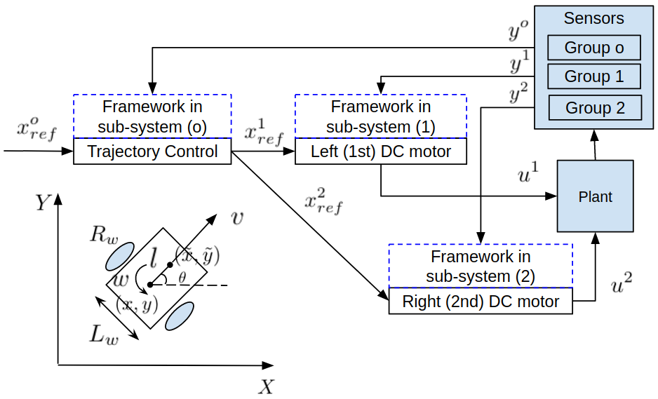
Figure 7. Bicycle model (bottom) & block diagram of controllers & framework (top-right) of a differential drive robot.

The system and framework of the differential drive ground robot can be represented by the block diagram shown in Figure 7. The ground robot has an outer trajectory control loop and two inner DC motor control loops. The outer loop provides reference values to both inner loops after transformation of outer control-inputs. The outer loop has a motion capture system. Both inner loops have encoders. The framework (and ADS) reads all sensors and provides updated state-estimates to each of the three controllers (demonstrating scalability).

The outer loop has the ground robot’s trajectory controller with bicycle dynamics as follows,

(23) $$x^{j}_{k+1} =\left(\begin{bmatrix}v_{k}\cos\theta_{k}&v_{k}\sin\theta_{k}&w_{k}\end{bmatrix}^{T}\right)\Delta T^{o}+\mathcal{N}(0,Q^{o})$$

with state $x^{j}_{k}=[x_{k},y_{k},\theta_{k}]^{T}$ (i.e. $x$, $y$ position and heading) and control inputs $u^{j}_{k}=[v_{k},w_{k}]^{T}$ (i.e. vel. and angular vel.) as shown in Figure 7. The outer loop employs sensors with the following model,

(24) $$y_{k}^{o}=x_{k}^{o}+\mathcal{N}(0,R^{o})$$

A dynamic inversion controller (based on first order dynamics) that considers a shifted state $l$ distance away (with $l\to 0$) is employed,

(25) $$\begin{bmatrix}v_{k}\\ w_{k}\end{bmatrix} =\begin{bmatrix}\cos\theta_{k}&\sin\theta_{k}\\ -\sin\theta_{k}/l&\cos\theta_{k}/l\end{bmatrix}\begin{bmatrix}\dot{x}_{k,ref}+k_{1}(x_{k,ref}-x)\\ \dot{y}_{k,ref}+k_{2}(y_{k,ref}-y_{k})\end{bmatrix}$$

The inner loops have PID controllers for the left and right DC motors with dynamics and control as follows (for $j=1,2$),

$$x^{j}_{k+1} =\left(\begin{bmatrix}-R/L&-K_{emf}/L\\ K_{tor}/J&-K_{fric}/J\end{bmatrix}x^{j}_{k}+\begin{bmatrix}1/L\\ 0\end{bmatrix}\mathrm{V}^{j}_{k}\right)\Delta T^{j}+\mathcal{N}(0,Q^{j})$$

(26) $$\mathrm{V}^{j}_{k} =PID(w^{j}_{k,ref}-w^{j}_{k})$$

with state $x^{j}_{k}=[i_{k},w_{k}]^{T}$ (i.e. current and angular velocity of motor) and control input $\mathrm{V}^{j}_{k}$ (i.e. voltage input to motor). The inner loops have measurement model as $y_{k}^{j}=\begin{bmatrix}0&1\end{bmatrix}x_{k}^{j}+\mathcal{N}(0,R^{j})$. Anomalous input of $[5,5,0]^{T}$ in $k=[3.25,5)$ and $-[5,5,0]^{T}$ in $k=[8.25,10)$ is fed to the outer loop sensors. In the same time-periods, anomalous input of $[20,000]$ and $[-20,000]$ is fed to both inner loops encoders. A specific ADS is assumed which provides list of state-estimates’ elements in all three loops that depend on anomalous sensors. This ADS has detection-time of $k=[3.25,3.5)\cup[8.25,8.5)$ for all three loops. The time-periods of the outer $dt^{o}$ and inner loops $dt^{1},dt^{2}$ are obtained as reciprocals of their chosen loop rates of 10 Hz and 100 Hz respectively. Checkpoints are created every second ($\mu=1$Hz).

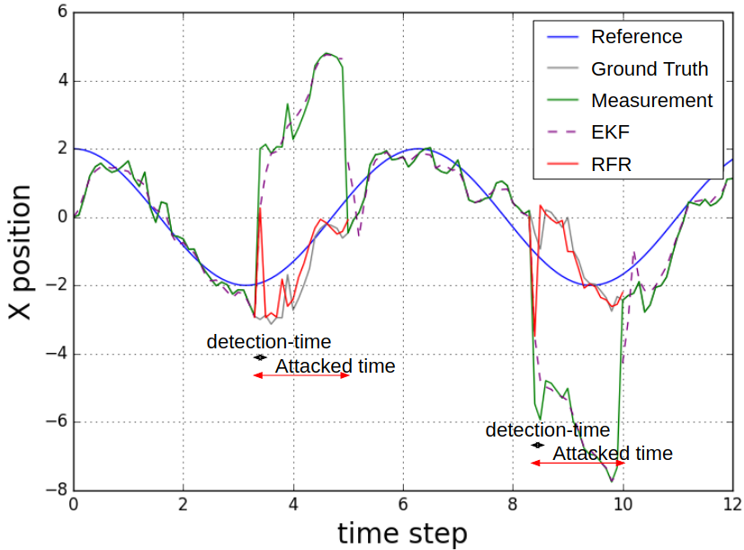
Figure 8. Time evolution of various robot x position series’

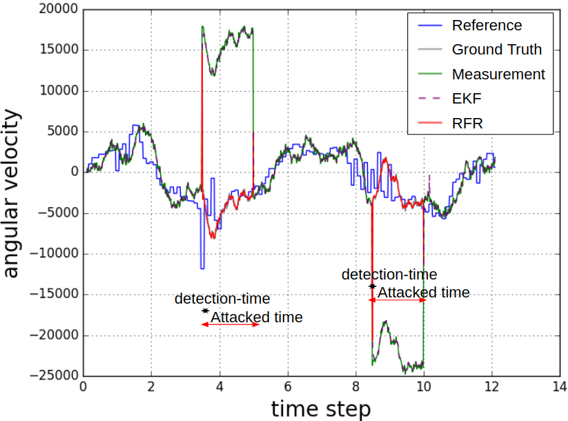
Figure 9. Time evolution of various left DC-motor $w$ series’

6.4. Simulation Results

In this subsection, we present and explain plots generated through numerical simulation. Figure 8 shows a plot of $x$ position of simulated ground robot vs time step and Figure 9 shows a plot of angular velocity of left DC motor vs time step. Plots of $y$ position of robot and angular velocity of right DC motor closely resemble the previously mentioned figures and so have not been shown.

In both Figures 8, 9, we see the ground truth (GT) state tracking the reference trajectory. Controller performance is thus assured. The EKF also tracks the ground truth when there is no anomaly but swerves to the false measurements (M) in the duration of the anomaly ($k=[3.25,5)\cup[8.25,10)$). The roll-forward value (RF), on the other hand, tracks the ground truth once the anomaly is detected ($k=[3.5,5)\cup[8.5,10)$). Thus, checkpointing and roll-forward recovery is shown to produce better state-estimates than an EKF during the anomalous time period.

Figure 10. Time evolution of errors & bounds in outer loop

Figure 11. Time evolution of errors, bounds in inner loop (1)

In the outer loop, and in the duration of the anomaly, we have RSEE & anomalous EKF estimate error (anomalous EE) for anomalous x position and estimation errors (EE) for healthy $\theta$ heading. This is shown in Figure 10. In the inner loops, and in the duration of the anomaly, we have RSEE & anomalous KF estimate error (anomalous EE) for anomalous angular velocity $w$ and estimation error (EE) for healthy current $i$. This is shown for the left DC motor in Figure 11. Both Figures 10, 11 also show the absolute bounds of EE and RSEE from Equation 15 and Proposition 5.1 / Corollary 5.2 resp.. Both RSEE and EE errors fall comfortably within their bounds. The anomalous EE is much larger than the RSEE for both x position and angular velocity $w$. This also shows that our framework performs better than an EKF in the presence of sensor anomalies.

7. Extension to Distributed Systems

In extending our work to distributed systems, we need to first ensure the reliability of communication, i.e. no messages are lost. We have to place scrutiny on the ADS monitoring the communication mechanism which presents as an added location for anomalies. Provided we have a reliable communication protocol on which anomalies can be accurately detected, then, we will have to focus on the time-delay caused by communication. A simple diagrammatic argument can show that if we assume communication lag ($\nu$) is bounded by the minimum of the inverse sub-system frequencies, i.e. $\nu\leq\min(\frac{1}{\mu^{in}},\frac{1}{\mu^{o}})$, then we can directly apply our framework to distributed systems. We will leave further extension of our framework to distributed systems in non-ideal conditions to future work.

8. Conclusion and Future Work

In conclusion, a framework for checkpointing and roll-forward recovery of state-estimates in nonlinear, hierarhical CPS with anomalous sensor data was proposed. The framework ensures consistent checkpointing with time-efficient roll-forward for diverse ADS in sub-systems. A tradeoff analysis between checkpointing frequency, accuracy and system resources was investigated and the related accuracy-resource gap bounded. Recovered state-estimate error bounds and maximum tolerable anomaly duration were also examined. A numerical evaluation showed scalability and better performance than a simple EKF. An extension to distributed systems under certain ideal conditions was discussed. In the future, a comprehensive extension to distributed systems can be completed.

 

Appendix A Appendix

A.1. Additional problem formulation details

A.1.1. Extended Kalman Filter:

The extended Kalman filter (EKF) is given as follows (with predict steps (27), (28), gain calculation (29) and update steps (30), (31)),

(27) $$\hat{x}^{j}_{k+1|k} =f^{j}(\hat{x}^{j}_{k},u^{j}_{k}),\;\;\;\;\;\hat{x}^{j}_{0}=x^{j}_{init},\;\;P^{j}_{0}=\Sigma^{j}$$

(28) $$P^{j}_{k+1|k} =A^{j}_{k}P^{j}_{k}{A^{j}_{k}}^{T}+Q^{j}$$

(29) $$K^{j}_{k} =P^{j}_{k+1|k}{C^{j}_{k}}^{T}(C^{j}_{k}P^{j}_{k+1|k}{C^{j}_{k}}^{T}+R^{j})^{-1}$$

(30) $$\hat{x}^{j}_{k+1} =\hat{x}^{j}_{k+1|k}+K^{j}_{k}(y^{j}_{k}-g^{j}(\hat{x}^{j}_{k+1|k},u^{j}_{k}))$$

(31) $$P^{j}_{k+1} =(I-K^{j}_{k}C^{j}_{k})P^{j}_{k+1|k}\;\;\;\;\;j\in\{in,o\}$$

where $A^{j}_{k}=\left.\frac{\partial f^{j}}{\partial x^{j}}\right|_{\hat{x}_{k},u_{k}}$ and $C^{j}_{k}=\left.\frac{\partial g^{j}}{\partial x^{j}}\right|_{\hat{x}_{k+1|k},u_{k}}$ are Jacobians.

A.2. Proof of Proposition 5.1

For the prediction error, we have by Equation (12),

$$e^{j}_{k+1,\ Rec} =\left[x^{j}_{k+1}-\hat{x}^{j,R}_{k+1}\right]_{(1,q)}$$

$$=\left[\left(f^{j}(x^{j}_{k},u^{j}_{k})+\omega^{j}_{k+1}\right)-f^{j}(\hat{x}^{j,R}_{k},u^{j}_{k})\right]_{(1,q)}$$

$$=\left[\left(f^{j}(x^{j}_{k},u^{j}_{k})-f^{j}(\hat{x}^{j,R}_{k},u^{j}_{k})\right)+\omega^{j}_{k+1}\right]_{(1,q)}$$

$$=\left[A_{k}\left(x^{j}_{k}-\hat{x}^{j,R}_{k}\right)+\varphi(x^{j}_{k},\hat{x}^{j,R}_{k},u^{j}_{k})+\omega^{j}_{k+1}\right]_{(1,q)}$$

$$=\left[A^{j}_{k}\left(f^{j}(x^{j}_{k-1},u^{j}_{k-1})-f^{j}(\hat{x}^{j,R}_{k-1},u^{j}_{k-1})\right)\right.$$

$$\left.+\omega^{j}_{k+1}+\varphi(x^{j}_{k},\hat{x}^{j,R}_{k},u^{j}_{k})\right]_{(1,q)}$$

where $\varphi(x^{j}_{k},\hat{x}^{j,R}_{k},u^{j}_{k})$ are the nonlinear terms from Taylor series expansion of $f^{j}(x^{j}_{k},u^{j}_{k})$ about $\hat{x}^{j,R}_{k}$.

By repeatedly using Taylor series expansions till checkpoint time ($k_{1}$), we have,

$$e^{j}_{k+1,\ Rec} =\left[\prod_{l=k_{1}}^{k}A^{j}_{l}\delta^{j}_{k_{1}}+\sum_{l=k_{1}}^{k}\prod_{m=l}^{k}(A^{j}_{m})\omega^{j}_{l}\right.$$

$$\left.+\omega^{j}_{k+1}+\Phi(x^{j}_{k},\hat{x}^{j,R}_{k},u^{j}_{k},...,x^{j}_{k_{1}},\bar{x}^{j}_{k_{1}},u^{j}_{k_{1}})\right]_{(1,q)}$$

where $\delta^{j}_{k_{1}}=\left(x^{j}_{k_{1}}-\bar{x}^{j}_{k_{1}}\right)$ can be obtained by a process similar to that described by Equations in (13).

$\Phi(x^{j}_{k},...,u^{j}_{k_{1}})$ represents the accumulated nonlinear terms after repeated Taylor series expansions. Finally, with the assumptions from Equations (14), (18), (19), we bound the prediction error as given in Equation (16). Hence proved Proposition 5.1.

A.3. Proof of Proposition 5.3

Since the recovered state-estimate error monotonically increases with time, it will reach the maximum permissible error $\mathbf{E}^{j}$ at some time $k$. We call the duration of time between the start of the attack at time $s$ and concerned time $k$, the maximum tolerable anomaly duration $T^{j}_{\max}$. Hence, we have $k=s+T^{j}_{\max}$. Then, given latest consistent checkpoint time before anomaly $k_{1}=\mathcal{F}^{j}(s,\Delta,\mu)$, we can find $T^{j}_{\max}$ by solving $\mathcal{B}(k,k_{1})=\mathbf{E}^{j}$ or equivalently the numerical minimization problem given in (21). This proves Proposition 5.3.

A.4. Proof of Proposition 5.4

The accuracy-resource gap $\mathcal{P}^{j}$ is given as

(32) $$\mathcal{P}^{j} =\hat{x}_{k,(1,q)}^{j,R}\Big{\rvert}_{\mu^{*}}-\hat{x}_{k,(1,q)}^{j,R}\Big{\rvert}_{\mu}$$

(33) $$=e^{j}_{k,\ Rec}\Bigg{\rvert}_{k_{1}=\ \mathcal{F}^{j}(s,\Delta,\mu)}-e^{j}_{k,\ Rec}\Bigg{\rvert}_{k_{1}=\ s-1=\ \mathcal{F}^{j}(s,\Delta,\mu^{*})}$$

(34) $$\leq\mathcal{B}(k,\mathcal{F}^{j}(s,\Delta,\mu))-\mathcal{B}(k,s-1)\;\;\;\;\;(\text{using }\eqref{pe_b},\eqref{Bound})$$

which proves Proposition 5.4.

Anomalies in sensors of subsystems $(o)$, $(in)$	Affected anomalous values	Solution or assumption for safe operation of CPS
detected, detected	$\hat{x}^{o}_{k}\to$ $u^{o}_{k}$; $\hat{x}^{in}_{k}\to$ $u^{in}_{k}$	roll-forward recovery (RFR) in both $(o),(in)$
detected, DNE	$\hat{x}^{o}_{k}\to$ $u^{o}_{k}\to$ $x^{in}_{k,ref}\to$ $u^{in}_{k}$	RFR in $(o)$
DNE, detected	$\hat{x}^{in}_{k}\to$ $u^{in}_{k}$	RFR in $(in)$
not yet detected, DNE	$\hat{x}^{o}_{k}\to$ $u^{o}_{k}\to$ $x^{in}_{k,ref}\to$ $u^{in}_{k}$	assume small value of $(o)$ detection time $\mathcal{T}^{o}_{k}$
DNE, not yet detected	$\hat{x}^{in}_{k}\to$ $u^{in}_{k}$	assume small value of $(in)$ detection time $\mathcal{T}^{in}_{k}$
detected, not yet detected	$\hat{x}^{o}_{k}\to$ $u^{o}_{k}$; $\hat{x}^{in}_{k}\to$ $u^{in}_{k}$	RFR in $(o)$ and assume small value of $\mathcal{T}^{in}_{k}$
not yet detected, detected	$\hat{x}^{o}_{k}\to$ $u^{o}_{k}$; $\hat{x}^{in}_{k}\to$ $u^{in}_{k}$	RFR in (in) and assume small value of $\mathcal{T}^{o}_{k}$
not yet detected, not yet detected	$\hat{x}^{o}_{k}\to$ $u^{o}_{k}$; $\hat{x}^{in}_{k}\to$ $u^{in}_{k}$	assume small bounds on $\mathcal{T}^{o}_{k},\mathcal{T}^{in}_{k}$
∗DNE = Do Not Exist.

Table 1. All possible combinations of cases of sensor anomalies in the hierarchy, the values they affect and the solution or assumption that addresses them.

A.5. Case-by-case analysis of anomalies in each sub-system

There are three cases for sensor anomalies in each sub-system: not yet detected anomalies, detected anomalies and no anomalies. The first induces detection error, the second leads to recovered state-estimate error and we have standard estimation error in all cases. We can have combinations of these three cases across the hierarchy and all such combinations are addressed by our framework. This is characterized by Table 1. It has 3 columns: the first column displays the anomaly situation in subsystems $(o),(in)$ respectively, the second column mentions which values are affected by sensor anomalies in each sub-system and the third column presents a solution or assumption for continued safe operation of the CPS.

In the first row, both sub-systems $(o)$ and $(in)$ have detected anomalies in sensors. This affects state estimates which in turn affect control values in both sub-systems (i.e. $\hat{x}^{j}_{k}\to u^{j}_{k}$ for $j=o,in$). For safe operation of CPS, we will have roll-forward recovery (abbreviated RFR) in both sub-systems $(o),(in)$. In the fourth row, we have anomalies in sub-system $(o)$ that are not yet detected and anomalies in sub-system $(in)$ that do not exist (i.e. no anomalies in $(in)$). The anomaly that hasn’t been detected in $(o)$ affects its state-estimates which affects the control inputs produced by $(o)$ which in turn affects the reference values sent by $(o)$ to $(in)$ which propagates to the control value generated by $(in)$ (i.e. $\hat{x}^{o}_{k}\to$ $u^{o}_{k}\to$ $x^{in}_{k,ref}\to$ $u^{in}_{k}$). For safe operation of CPS in this case, we assume a small detection time. The other rows in the table can be similarly interpreted.

A.6. More details and results for case-study

A.6.1. Additional details for problem formulation in the case-study of a simulated differential drive ground robot

We have for the outer loop

(35) $$x^{o}_{ref}=\begin{bmatrix}2\cos(k)&2\sin(k)&\tan^{-1}\left(\frac{2\sin(k)-y_{k}}{2\cos(k)-x_{k}}\right)\end{bmatrix}^{T}$$

(36) $$A^{o}_{k}=\begin{bmatrix}0&0&-v_{k}\sin\theta_{k}\\ 0&0&v_{k}\cos\theta_{k}\\ 0&0&0\end{bmatrix},\Gamma^{o}=\begin{bmatrix}1&0&0\\ 0&1&0\\ 0&0&0\end{bmatrix}$$

(37) $$G^{o}_{k}=\begin{cases}[1,1,0]^{T},\;k\in[3.5,5)\cup[8.5,10)\\ [0,0,0]^{T},\text{otherwise}\end{cases}$$

(38) $$x^{1}_{ref}=w^{1}_{k,ref}\in\mathbb{R},x^{2}_{ref}=w^{2}_{k,ref}\in\mathbb{R}$$

(39) $$T(u^{o}_{k})=\begin{bmatrix}w^{1}_{k,ref}\\ w^{2}_{k,ref}\end{bmatrix}=\begin{bmatrix}\frac{2v-\omega L_{w}}{2R_{w}}&\frac{2v+\omega L_{w}}{2R_{w}}\end{bmatrix}^{T}$$

where, at time $k$, $w^{1}_{k,ref},w^{2}_{k,ref}$ represent reference angular vel. sent by outer loop to 1st and 2nd DC motor controllers resp., radius of wheel is $R_{w}=0.05$m and length between wheels is $L_{w}=0.5$m. We also assume $Q^{o}=R^{o}=(0.1)^{2}\mathbf{I}_{3\times 3}$

Next, we have for the inner loops ($j=1,2$),

(40) $$G^{j}_{k}=\begin{cases}\begin{bmatrix}0&1\end{bmatrix}^{T},\;k\in[3.5,5)\cup[8.5,10)\\ \begin{bmatrix}0&0\end{bmatrix}^{T},\text{otherwise}\end{cases}$$

and we have resistance $R=1\Omega$, self-inductance $L=0.5$H, armature, emf and viscous friction coefficients $K_{tor}=K_{emf}=K_{fric}=0.01$ and inertial load $J=0.01$ of the DC motor. We also have gains of the PID controller $K_{p}=13.2$, $K_{d}=0.275$ and $K_{i}=1.525$. Lastly, we assume $Q^{1}=Q^{2}=(50)^{2}\mathbf{I}_{2\times 2}$ and $R^{1}=R^{2}=(50)^{2}$.

Figure 12. Checkpoints used for roll-forward vs time step (blue) and checkpoint creation (orange) in the ground robot’s trajectory control outer loop

A.6.2. Checkpointing in the case-study

Figure 12 represents the checkpointing process for the robot trajectory controller. The orange points represent checkpoints that were created at a time step given by either their x or y coordinates on the plot. The blue points represent checkpoints that were created at time step given by their y coordinate and used for roll-forward recovery at time step given by their x coordinate. Since the inner loops run faster than the outer loop, we would see more blue points in the plots for the DC motor but no other difference and so they are not shown here.

References

- (1)
- cle (2013) 2013. A Clever Trigonometry Based Dynamic Inversion Controller. http://faculty.salina.k-state.edu/tim/robotics_sg/Control/controllers/trig_trick.html (2013).
- Bu et al. (2017) J. Bu, R. Sun, H. Bai, R. Xu, F. Xie, Y. Zhang, and W.Y. Ochieng. 2017. Integrated method for the UAV navigation sensor anomaly detection. IET Radar, Sonar & Navigation 11, 5 (2017), 847–853.
- Guo et al. (2018) P. Guo, H. Kim, N. Virani, J. Xu, M. Zhu, and P. Liu. 2018. RoboADS: Anomaly detection against sensor and actuator misbehaviors in mobile robots. In 2018 48th Annual IEEE/IFIP International Conference on Dependable Systems and Networks.
- Ivanov et al. (2019) R. Ivanov, T. J. Carpenter, J. Weimer, R. Alur, G. J Pappas, and I. Lee. 2019. Case Study: Verifying the Safety of an Autonomous Racing Car with a Neural Network Controller. arXiv preprint arXiv:1910.11309 (2019).
- Kong et al. (2018) F. Kong, M. Xu, J. Weimer, O. Sokolsky, and I. Lee. 2018. Cyber-Physical System Checkpointing and Recovery. In Proceedings of the 9th ACM/IEEE International Conference on Cyber-Physical Systems (ICCPS ’18). IEEE Press, 22–31.
- Kong et al. (2015) J. Kong, M. Pfeiffer, G. Schildbach, and F. Borrelli. 2015. Kinematic and dynamic vehicle models for autonomous driving control design. In 2015 IEEE Intelligent Vehicles Symposium (IV). IEEE, 1094–1099.
- Kopetz (2011) H. Kopetz. 2011. Real-time systems: design principles for distributed embedded applications. Springer Science & Business Media, 51–77.
- Manabe (2001) Y. Manabe. 2001. A distributed consistent global checkpoint algorithm for distributed mobile systems. In Proceedings. Eighth International Conference on Parallel and Distributed Systems. ICPADS 2001. 125–132.
- Miao et al. (2013) F. Miao, M. Pajic, and G. J. Pappas. 2013. Stochastic game approach for replay attack detection. In 52nd IEEE conference on decision and control. IEEE, 1854–1859.
- Mo and Sinopoli (2010) Y. Mo and B. Sinopoli. 2010. False data injection attacks in control systems. In Preprints of the 1st workshop on Secure Control Systems. 1–6.
- Ni et al. (2009) K. Ni, N. Ramanathan, M. N. Chehade, L. Balzano, S. Nair, S.and Zahedi, E. Kohler, G. Pottie, M. Hansen, and M. Srivastava. 2009. Sensor network data fault types. ACM Transactions on Sensor Networks (TOSN) 5, 3 (2009), 1–29.
- Pajic et al. (2014) M. Pajic, J. Weimer, N. Bezzo, P. Tabuada, O. Sokolsky, I. Lee, and G. J. Pappas. 2014. Robustness of attack-resilient state estimators. In 2014 ACM/IEEE International Conference on Cyber-Physical Systems (ICCPS). IEEE, 163–174.
- Park et al. (2015) J. Park, R. Ivanov, J. Weimer, and I. Pajic, M.and Lee. 2015. Sensor attack detection in the presence of transient faults. In Proceedings of the ACM/IEEE Sixth International Conference on Cyber-Physical Systems. 1–10.
- Petit et al. (2015) J. Petit, B. Stottelaar, M. Feiri, and F. Kargl. 2015. Remote attacks on automated vehicles sensors: Experiments on camera and lidar. Black Hat Europe 11 (2015).
- Rajamani (2011) R. Rajamani. 2011. Vehicle Dynamics & Control. Springer.
- Rutkin (2013) A.H. Rutkin. 2013. spoofers use fake GPS signals to knock a yacht off course. MIT Technology Review (2013).
- Sharma et al. (2010) A. B. Sharma, L. Golubchik, and R. Govindan. 2010. Sensor faults: Detection methods and prevalence in real-world datasets. ACM Transactions on Sensor Networks (TOSN) 6, 3 (2010), 1–39.
- Shoukry et al. (2017) Y. Shoukry, P. Nuzzo, A. Puggelli, A.L. S.-Vincentelli, S.A. Seshia, and P. Tabuada. 2017. Secure state estimation for cyber-physical systems under sensor attacks: A satisfiability modulo theory approach. IEEE Trans. Automat. Control (2017).
- et al. (2011) P. G. Jacobs et al. 2011. Development of a fully automated closed loop artificial pancreas control system with dual pump delivery of insulin and glucagon. In 2011 Annual International Conference of the IEEE Engineering in Medicine and Biology Society. 397–400.
- van Wyk et al. (2019) F. van Wyk, Y. Wang, A. Khojandi, and N. Masoud. 2019. Real-time sensor anomaly detection and identification in automated vehicles. IEEE Transactions on Intelligent Transportation Systems 21, 3 (2019), 1264–1276.