DPO: Dynamic-Programming Optimization on Hybrid Constraints

Abstract

In Bayesian inference, the most probable explanation (MPE) problem requests a variable instantiation with the highest probability given some evidence. Since a Bayesian network can be encoded as a literal-weighted CNF formula $\varphi$, we study Boolean MPE, a more general problem that requests a model $\tau$ of $\varphi$ with the highest weight, where the weight of $\tau$ is the product of weights of literals satisfied by $\tau$. It is known that Boolean MPE can be solved via reduction to (weighted partial) MaxSAT. Recent work proposed DPMC, a dynamic-programming model counter that leverages graph-decomposition techniques to construct project-join trees. A project-join tree is an execution plan that specifies how to conjoin clauses and project out variables. We build on DPMC and introduce DPO, a dynamic-programming optimizer that exactly solves Boolean MPE. By using algebraic decision diagrams (ADDs) to represent pseudo-Boolean (PB) functions, DPO is able to handle disjunctive clauses as well as XOR clauses. (Cardinality constraints and PB constraints may also be compactly represented by ADDs, so one can further extend DPO’s support for hybrid inputs.) To test the competitiveness of DPO, we generate random XOR-CNF formulas. On these hybrid benchmarks, DPO significantly outperforms MaxHS, UWrMaxSat, and GaussMaxHS, which are state-of-the-art exact solvers for MaxSAT.

1 Introduction

Bayesian inference [Pearl, 1985] has numerous applications, including medical diagnosis [Shwe et al., 1991] and industrial fault analysis [Cai et al., 2017]. Given a Bayesian network, the most probable explanation (MPE) problem requests a variable instantiation with the highest probability. MPE has the form $\operatorname*{argmax}_{X}f\left(X\right)$, where $f$ is a real-valued function over a set $X$ of variables. Also having that form is the satisfiability (SAT) problem, which requests a satisfying truth assignment (model) of a Boolean formula [Cook, 1971]. SAT can be viewed as a counterpart of MPE where $f$ is a Boolean function [Littman et al., 2001].

A generalization of SAT is the Boolean MPE problem, which receives a literal-weighted Boolean formula and requests a maximizing truth assignment (maximizer), i.e., a truth assignment $\tau$ with the highest weight, where the weight of $\tau$ is the product of weights of literals satisfied by $\tau$ [Sang et al., 2007]. Boolean MPE is more general than (Bayesian) MPE because Bayesian networks can be encoded as literal-weighted Boolean formulas [Sang et al., 2005].

A Boolean formula is usually given in conjunctive normal form (CNF), i.e., as a set of disjunctive clauses. An optimization version of SAT, the maximum satisfiability (MaxSAT) problem, requests a truth assignment that maximizes the number of satisfied clauses of an unsatisfiable CNF formula [Krentel, 1988]. MaxSAT may be used to solve MPE [Park, 2002] and Boolean MPE [Sang et al., 2007] via appropriate reductions.

Most SAT and MaxSAT solvers only accept Boolean formulas in CNF, but disjunctive clauses do not always provide a natural formulation of an application. For example, certain properties in cryptography are more conveniently described with XOR [Bogdanov et al., 2011]. In addition, cardinality constraints help formulate problems in graph coloring [Costa et al., 2009], and hybrid constraints have also been used for maximum-likelihood decoding [Feldman et al., 2005].

All Boolean constraints can be converted into CNF, and efficient CNF encodings often exist. For example, XOR can be encoded using the Tseitin transformation, which adds a linear number of disjunctive clauses and auxiliary variables [Tseitin, 1983]. There are, however, many possible CNF encodings, and solver performance crucially depends on the encoding used, so finding good encodings is solver-dependent and nontrivial [Prestwich, 2009]. Thus, CNF conversion is not always a good approach when dealing with hybrid constraints.

Instead of using CNF encodings, one may wish to handle non-disjunctive constraints natively. This direct approach avoids conversion overhead and preserves application-specific structure that would be hard to recover after transformation. Hybrid solvers have been developed for SAT [Soos et al., 2009, Yang and Meel, 2021] and related problems, such as weighted model counting (WMC) [Soos and Meel, 2019, Soos et al., 2020]. (WMC requests the sum of weights of satisfying truth assignments of a Boolean formula [Valiant, 1979].) Yet developing performant hybrid solvers for specific types of non-disjunctive constraints is labor-intensive, which motivates the need for hybrid solvers that can natively handle a variety of constraint types, e.g., [Kyrillidis et al., 2020].

A recent WMC framework is DPMC [Dudek et al., 2020], which employs dynamic programming, a strategy that solves a large instance by decomposing it into parts then combining partial solutions into a final answer. Dynamic programming has been applied to WMC [Fichte et al., 2020, Dudek et al., 2021], SAT [Pan and Vardi, 2005], MaxSAT [Sang et al., 2007, Saether et al., 2015], and quantified Boolean formula (QBF) evaluation [Charwat and Woltran, 2016].

To guide dynamic programming for WMC, DPMC uses project-join trees as execution plans. A project-join tree for a CNF formula specifies how to conjoin clauses and project out variables in order to obtain the weighted model count. DPMC operates in two phases. First, the planning phase builds a project-join tree with graph-decomposition techniques [Robertson and Seymour, 1991, Strasser, 2017]. Second, the execution phase uses the built tree to compute a final answer, where intermediate results are represented by algebraic decision diagrams (ADDs) [Bahar et al., 1997, Somenzi, 2015]. ADDs are a data structure that compactly represents pseudo-Boolean functions, such as conjunction, disjunction, XOR, cardinality constraints, and others.

We build on DPMC to develop DPO, a dynamic-programming optimization framework that exactly solves Boolean MPE on XOR-CNF formulas. To find maximizers, we also adapt an iterative technique [Kyrillidis et al., 2022] that was recently proposed for MaxSAT. To demonstrate the advantage of our approach, we generate random XOR-CNF benchmarks on which DPO significantly outperforms MaxHS [Davies and Bacchus, 2011], UWrMaxSat [Piotrow, 2020], and GaussMaxHS [Soos and Meel, 2021], which are state-of-the-art exact solvers for MaxSAT.

2 Related Work

MPE-SAT [Sang et al., 2007] is an exact Boolean MPE solver that is based on DPLL and techniques in WMC [Sang et al., 2004]. MPE-SAT dynamically detects connected components, which are subformulas with disjoint sets of variables. These components can be solved independently before results are combined into a final answer. Processed components and their computed values are cached to avoid repeated work. A lower bound is dynamically updated to prune the search tree. MPE-SAT also utilizes CDCL to eliminate the infeasible search space.

Instead of solving Boolean MPE directly, one can employ a simple reduction from a Boolean MPE instance $\varphi$ to a (weighted partial) MaxSAT instance $\psi$ [Sang et al., 2007]. First, each clause of the original CNF formula $\varphi$ induces a hard clause of the new CNF formula $\psi$. Then, each literal $l$ of $\varphi$ with weight $w$ induces a unit clause $l$ of $\psi$ with soft weight $\log\left(w\right)$. If $\varphi$ has $n$ variables and $m$ clauses, then $\psi$ has $n$ variables, $m$ hard clauses, and $2n$ soft clauses. Notice that a truth assignment $\tau$ is a maximizer of $\varphi$ if and only if $\tau$ is an optimal truth assignment of $\psi$.

There are several MaxSAT algorithms that cover a variety of techniques [Bacchus et al., 2020]. For example, MaxHS combines SAT and hitting-set computation [Davies and Bacchus, 2011]. In more detail, MaxHS invokes a SAT solver to find unsatisfiable cores. To compute a minimal-cost hitting set, MaxHS employs integer linear programming (ILP) as well as a branch-and-bound approach. A more recent MaxSAT solver is UWrMaxSat [Piotrow, 2020], which also solves PB problems. UWrMaxSat uses a core-guided approach and translates cardinality constraints into CNF. For weighted instances, UWrMaxSat applies other techniques as well, such as preprocessing to detect unit cores. An extension of UWrMaxSat is CASHWMaxSAT [Lei et al., 2021], which transforms small MaxSAT instances into ILP. Also, CASHWMaxSAT invokes a SAT solver multiple times to find smaller cores. After choosing a core, CASHWMaxSAT delays encoding the new constraint if the core is larger than a predefined threshold.

Most MaxSAT solvers only work on CNF, but GaussMaxHS [Soos and Meel, 2021] also supports XOR clauses. Inspired by the SAT solver CryptoMiniSat [Soos et al., 2009], GaussMaxHS uses an architecture that combines Gaussian elimination with the MaxSAT solver MaxHS. Gaussian elimination is performed on dense bit-packed matrices to exploit SIMD. A related XOR-CNF architecture has been proposed for approximate WMC [Soos and Meel, 2019].

3 Preliminaries

3.1 Graphs

In a graph $G$, let $\mathcal{V}\left(G\right)$ denote the set of vertices. A tree is an undirected graph that is connected and acyclic. We refer to a vertex of a tree as a node. A rooted tree is a tree $T$ together with a distinguished node $r\in\mathcal{V}\left(T\right)$ called the root. In a rooted tree $\langle T,r\rangle$, each node $v\in\mathcal{V}\left(T\right)$ has a (possibly empty) set of children, denoted by $\mathcal{C}\left(T,r,v\right)$, which contains every node $v^{\prime}$ adjacent to $v$ such that the path from $v^{\prime}$ to $r$ passes through $v$. A leaf of a rooted tree $\langle T,r\rangle$ is a non-root node of degree one. Let $\mathcal{L}\left(T,r\right)$ denote the set of leaves of $\langle T,r\rangle$. An internal node is a member of $\mathcal{V}\left(T\right)\setminus\mathcal{L}\left(T,r\right)$, including the root.

3.2 Pseudo-Boolean Functions

Let $B^{A}$ denote the set of all functions $f$ with domain $\operatorname{dom}\left(f\right):=A$ and codomain $B$. The restriction of $f$ to a set $S$ is a function defined by $f\restriction_{S}:=\left\{\langle a,b\rangle\in f\mid a\in S\right\}$.

From now on, every variable is binary unless noted otherwise. A truth assignment for a set $X$ of variables is a function $\tau:X\to\mathbb{B}$.

A pseudo-Boolean (PB) function over a set $X$ of variables is a function $f:\mathbb{B}^{X}\to\mathbb{R}$. Define $\operatorname{vars}\left(f\right):=X$. We say that $f$ is constant if $X=\varnothing$. A Boolean function is a special PB function $f:\mathbb{B}^{X}\to\mathbb{B}$.

Definition 1 (Join).

Let $f:\mathbb{B}^{X}\to\mathbb{R}$ and $g:\mathbb{B}^{Y}\to\mathbb{R}$ be PB functions. The (multiplicative) join of $f$ and $g$ is a PB function, denoted by $f\cdot g:\mathbb{B}^{X\cup Y}\to\mathbb{R}$, defined for each $\tau\in\mathbb{B}^{X\cup Y}$ by $(f\cdot g)(\tau):=f(\tau\restriction_{X})\cdot g(\tau\restriction_{Y})$.

Join is commutative and associative: we have $f\cdot g=g\cdot f$ as well as $(f\cdot g)\cdot h=f\cdot(g\cdot h)$ for all PB functions $f$, $g$, and $h$. Then define $\prod_{i=1}^{n}f_{i}:=f_{1}\cdot f_{2}\cdot\ldots\cdot f_{n}$.

Definition 2 (Existential Projection).

Let $f:\mathbb{B}^{X}\to\mathbb{R}$ be a PB function and $x$ be a variable. The existential projection of $f$ w.r.t. $x$ is a PB function, denoted by $\exists_{x}f:\mathbb{B}^{X\setminus\left\{x\right\}}\to\mathbb{R}$, defined for each $\tau\in\mathbb{B}^{X\setminus\left\{x\right\}}$ by $(\exists_{x}f)(\tau):=\max\left(f(\tau\cup\left\{\langle x,0\rangle\right\}),f(\tau\cup\left\{\langle x,1\rangle\right\})\right)$.

Existential projection is commutative: $\exists_{x}(\exists_{y}f)=\exists_{y}(\exists_{x}f)$ for all variables $x$ and $y$. Then define $\exists_{S}f:=\exists_{x}\exists_{y}\ldots f$, where $S=\left\{x,y,\ldots\right\}$ is a set of variables. By convention, $\exists_{\varnothing}f:=f$.

Definition 3 (Maximum).

Let $f:\mathbb{B}^{X}\to\mathbb{R}$ be a PB function. The maximum of $f$ is the real number $(\exists_{X}f)(\varnothing)$.

Definition 4 (Maximizer).

Let $f:\mathbb{B}^{X}\to\mathbb{R}$ be a PB function. A maximizer of $f$ is a truth assignment $\tau\in\mathbb{B}^{X}$ such that $f(\tau)=(\exists_{X}f)(\varnothing)$.

Another type of projection, also widely used in propositional logic, is defined as follows.

Definition 5 (Additive Projection).

Let $f:\mathbb{B}^{X}\to\mathbb{R}$ be a PB function and $x$ be a variable. The additive projection of $f$ w.r.t. $x$ is a PB function, denoted by $\Sigma_{x}f:\mathbb{B}^{X\setminus\left\{x\right\}}\to\mathbb{R}$, defined for each $\tau\in\mathbb{B}^{X\setminus\left\{x\right\}}$ by $(\Sigma_{x}f)(\tau):=f(\tau\cup\left\{\langle x,0\rangle\right\})+f(\tau\cup\left\{\langle x,1\rangle\right\})$.

Additive projection is commutative: $\Sigma_{x}(\Sigma_{y}f)=\Sigma_{y}(\Sigma_{x}f)$ for all variables $x$ and $y$. Then define $\Sigma_{S}f:=\Sigma_{x}\Sigma_{y}\ldots f$, where $S=\left\{x,y,\ldots\right\}$ is a set of variables. By convention, $\Sigma_{\varnothing}f:=f$.

Propositional logic can be generalized for probabilistic domains using real-valued weights.

Definition 6 (Literal-Weight Function).

A literal-weight function over a set $X$ of variables is a PB function, denoted by $W:\mathbb{B}^{X}\to\mathbb{R}$, defined by $W:=\prod_{x\in X}W_{x}$ for some PB functions $W_{x}:\mathbb{B}^{\left\{x\right\}}\to\mathbb{R}$.

3.3 Boolean MPE

Given a Boolean formula $\varphi$, define $\operatorname{vars}\left(\varphi\right)$ to be the set of all variables that appear in $\varphi$. Then $\varphi$ represents a Boolean function, denoted by $\left[\varphi\right]:\mathbb{B}^{\operatorname{vars}\left(\varphi\right)}\to\mathbb{B}$, defined according to standard Boolean semantics.

Definition 7 (Boolean MPE).

Let $\varphi$ be a Boolean formula and $W$ be a literal-weight function over $\operatorname{vars}\left(\varphi\right)$. The Boolean MPE problem on $\langle\varphi,W\rangle$ requests the maximum and a maximizer of $\left[\varphi\right]\cdot W$.

We also formally define the following related problem.

Definition 8 (Weighted Model Counting).

Let $\varphi$ be a Boolean formula and $W$ be a literal-weight function over $X=\operatorname{vars}\left(\varphi\right)$. The weighted model counting (WMC) problem on $\langle\varphi,W\rangle$ requests the real number $\left(\Sigma_{X}\left(\left[\varphi\right]\cdot W\right)\right)(\varnothing)$.

4 Solving Boolean MPE

4.1 Monolithic Approach

A Boolean formula is usually given in conjunctive normal form (CNF), i.e., as a set of clauses. We work with a more general format, XOR-CNF, in which a clause is an XOR or a disjunction of literals.

Given an XOR-CNF formula $\varphi$, we have the factorization $\left[\varphi\right]=\prod_{c\in\varphi}\left[c\right]$. In this section, we present an inefficient algorithm to solve Boolean MPE that treats $\varphi$ as a monolithic structure and ignores the XOR-CNF factored representation. The next section describes a more efficient algorithm.

To find maximizers for Boolean MPE, we leverage the following idea, which originated from the basic algorithm for PB programming [Crama et al., 1990] and was adapted for MaxSAT [Kyrillidis et al., 2022].

Definition 9 (Derivative Sign).

Let $f:\mathbb{B}^{X}\to\mathbb{R}$ be a PB function and $x$ be a variable. The derivative sign of $f$ w.r.t. $x$ is a function, denoted by $\operatorname*{dsgn}_{x}f:\mathbb{B}^{X\setminus\left\{x\right\}}\to\mathbb{B}^{\left\{x\right\}}$, defined for each $\tau\in\mathbb{B}^{X\setminus\left\{x\right\}}$ by $\left(\operatorname*{dsgn}_{x}f\right)(\tau):=\left\{\langle x,1\rangle\right\}$ if $f(\tau\cup\left\{\langle x,1\rangle\right\})\geq f(\tau\cup\left\{\langle x,0\rangle\right\})$, and $\left(\operatorname*{dsgn}_{x}f\right)(\tau):=\left\{\langle x,0\rangle\right\}$ otherwise.

The following result leads to an iterative process to find maximizers of PB functions [Kyrillidis et al., 2022].

Proposition 1 (Iterative Maximization).

Let $f:\mathbb{B}^{X}\to\mathbb{R}$ be a PB function and $x$ be a variable. Assume that a truth assignment $\tau$ is a maximizer of $\exists_{x}f:\mathbb{B}^{X\setminus\left\{x\right\}}\to\mathbb{R}$. Then the truth assignment $\tau\cup\left(\operatorname*{dsgn}_{x}f\right)(\tau)$ is a maximizer of $f$.

algorithm 1 can be used to find maximizers [Kyrillidis et al., 2022].

Input: $f_{n}$: a PB function over a set $X_{n}=\left\{x_{1},x_{2},\ldots,x_{n}\right\}$ of variables

Output: $m\in\mathbb{R}$: the maximum of $f_{n}$

Output: $\tau_{n}\in\mathbb{B}^{X_{n}}$: a maximizer of $f_{n}$

1

2for $i=n,n-1,\ldots,2,1$ 

       $f_{i-1}\leftarrow\exists_{x_{i}}f_{i}$ // $f_{i}$ is a PB function over $X_{i}=\left\{x_{1},x_{2},\ldots,x_{i}\right\}$

3      

4

$m\leftarrow f_{0}(\varnothing)$ // $f_{0}=\exists_{X_{n}}f_{n}$ is a constant PB function over $X_{0}=\varnothing$

$\tau_{0}\leftarrow\varnothing$ // $\tau_{0}$ is a maximizer of $f_{0}$ (and also the only input to $f_{0}$)

5 for $i=1,2,\ldots,n-1,n$ 

       $\tau_{i}\leftarrow\tau_{i-1}\cup\left(\operatorname*{dsgn}_{x_{i}}f_{i}\right)(\tau_{i-1})$ // $\tau_{i}$ is a maximizer of $f_{i}$ since $\tau_{i-1}$ is a maximizer of $f_{i-1}$ (by proposition 1)

6      

7

return $\langle m,\tau_{n}\rangle$

Algorithm 1 Computing the maximum and a maximizer of a PB function

algorithm 1 can be used to find maximizers [Kyrillidis et al., 2022].

Proposition 2 (Correctness of algorithm 1).

Let $\varphi$ be a Boolean formula and $W$ be a literal-weight function over $\operatorname{vars}\left(\varphi\right)$. algorithm 1 solves Boolean MPE on $\langle\varphi,W\rangle$ given the input $f_{n}=\left[\varphi\right]\cdot W$.

Boolean MPE on $\langle\varphi,W\rangle$ can be solved by calling algorithm 1 with $\left[\varphi\right]\cdot W$ as an input. But the PB function $\left[\varphi\right]\cdot W$ may be too large to fit in main memory, making the computation slow or even impossible. In the next section, we exploit the XOR-CNF factorization of $\varphi$ and propose a more efficient solution.

4.2 Dynamic Programming

Boolean MPE on $\langle\varphi,W\rangle$ involves the PB function $\left[\varphi\right]\cdot W=\prod_{c\in\varphi}\left[c\right]\cdot\prod_{x\in X}W_{x}$, where $\varphi$ is an XOR-CNF formula and $W$ is a literal-weight function over $X=\operatorname{vars}\left(\varphi\right)$. Instead of projecting all variables in $X$ after joining all clauses, we can be more efficient and project some variables early as follows [Dudek et al., 2021].

Proposition 3 (Early Projection).

Let $f:\mathbb{B}^{X}\to\mathbb{R}$ and $g:\mathbb{B}^{Y}\to\mathbb{R}$ be PB functions. Then for all $S\subseteq X\setminus Y$, we have $\exists_{S}(f\cdot g)=(\exists_{S}f)\cdot g$ and $\Sigma_{S}(f\cdot g)=(\Sigma_{S}f)\cdot g$.

Early projection can lead to smaller intermediate PB functions. For example, the bottleneck in computing $\exists_{S}(f\cdot g)$ is $f\cdot g$ with size $s=\left|\operatorname{vars}\left(f\cdot g\right)\right|=\left|X\cup Y\right|$. The bottleneck in computing $(\exists_{S}f)\cdot g$ is $f$ with size $s_{1}=\left|\operatorname{vars}\left(f\right)\right|=\left|X\right|$ or is $(\exists_{S}f)\cdot g$ with size $s_{2}=\left|\operatorname{vars}\left((\exists_{S}f)\cdot g\right)\right|=\left|X\cup Y\setminus S\right|$. Notice that $s\geq\max(s_{1},s_{2})$. The difference is consequential since an operation on a PB function $h$ may take $\operatorname{O}\left(2^{\left|\operatorname{vars}\left(h\right)\right|}\right)$ time and space.

We can apply early projection systematically by adapting the following framework, DPMC, which uses dynamic programming for WMC on CNF formulas [Dudek et al., 2020].

Definition 10 (Project-Join Tree).

Let $\varphi$ be an XOR-CNF formula (i.e., a set of XOR clauses and disjunctive clauses). A project-join tree for $\varphi$ is a tuple $\mathcal{T}=\langle T,r,\gamma,\pi\rangle$, where:

• $\langle T,r\rangle$ is a rooted tree,

• $\gamma:\mathcal{L}\left(T,r\right)\to\varphi$ is a bijection, and

• $\pi:\mathcal{V}\left(T\right)\setminus\mathcal{L}\left(T,r\right)\to\mathbb{B}^{\operatorname{vars}\left(\varphi\right)}$ is a function.

A project-join must satisfy the following criteria:

1. The set $\left\{\pi(v)\mid v\in\mathcal{V}\left(T\right)\setminus\mathcal{L}\left(T,r\right)\right\}$ is a partition of $\operatorname{vars}\left(\varphi\right)$, where some $\pi(v)$ sets may be empty.

2. For each internal node $v$, variable $x\in\pi(v)$, and clause $c\in\varphi$, if $x\in\operatorname{vars}\left(c\right)$, then the leaf $\gamma^{-1}\left(c\right)$ is a descendant of $v$ in $\langle T,r\rangle$.

For a leaf $v\in\mathcal{L}\left(T,r\right)$, define $\operatorname{vars}\left(v\right):=\operatorname{vars}\left(\gamma(v)\right)$, i.e., the set of variables that appear in the clause $\gamma(v)\in\varphi$. For an internal node $v\in\mathcal{V}\left(T\right)\setminus\mathcal{L}\left(T,r\right)$, define $\operatorname{vars}\left(v\right):=\left(\bigcup_{v^{\prime}\in\mathcal{C}\left(T,r,v\right)}\operatorname{vars}\left(v^{\prime}\right)\right)\setminus\pi(v)$.

figure 1 illustrates a project-join tree.

Figure 1: A project-join tree $\mathcal{T}=\langle T,n_{10},\gamma,\pi\rangle$ for an XOR-CNF formula $\varphi$. Each leaf corresponds to a clause of $\varphi$ under $\gamma$. Each internal node corresponds to a set of variables of $\varphi$ under $\pi$.

We adapt the following definition for Boolean MPE on XOR-CNF [Dudek et al., 2020].

Definition 11 (Valuation of Project-Join Tree Node).

Let $\varphi$ be an XOR-CNF formula, $\langle T,r,\gamma,\pi\rangle$ be a project-join tree for $\varphi$, and $W$ be a literal-weight function over $\operatorname{vars}\left(\varphi\right)$. The $W$-valuation of $v\in\mathcal{V}\left(T\right)$ is a PB function, denoted by ${\llbracket v\rrbracket}_{W}:\mathbb{B}^{\operatorname{vars}\left(v\right)}\to\mathbb{R}$, defined by the following:

$${\llbracket v\rrbracket}_{W}:=\begin{cases}\left[\gamma(v)\right]&\text{if }v\in\mathcal{L}\left(T,r\right)\\ \displaystyle\operatorname*{\vphantom{\sum}\mathchoice{\vbox{\hbox{$\exists$}}}{\vbox{\hbox{$\exists$}}}{\vbox{\hbox{$\exists$}}}{\vbox{\hbox{$\exists$}}}}_{\pi(v)}\left(\prod_{v^{\prime}\in\mathcal{C}\left(T,r,v\right)}{\llbracket v^{\prime}\rrbracket}_{W}\cdot\prod_{x\in\pi(n)}W_{x}\right)&\text{otherwise}\end{cases}$$

Recall that $\left[\gamma(v)\right]$ is the Boolean function represented by the clause $\gamma(v)\in\varphi$. Also, ${\llbracket v^{\prime}\rrbracket}_{W}$ is the $W$-valuation of a child $v^{\prime}$ of the node $v$ in the rooted tree $\langle T,r\rangle$. Note that the $W$-valuation of the root $r$ is a constant PB function.

Definition 12 (Width of Project-Join Tree).

Let $\mathcal{T}=\langle T,r,\gamma,\pi\rangle$ be a project-join tree. For a leaf $v$ of $\mathcal{T}$, define $0pt{v}:=\left|\operatorname{vars}\left(v\right)\right|$. For an internal node $v$ of $\mathcal{T}$, define $0pt{v}:=\left|\operatorname{vars}\left(v\right)\cup\pi(v)\right|$. The width of $\mathcal{T}$ is $0pt{\mathcal{T}}:=\max_{v\in\mathcal{V}\left(T\right)}0pt{v}$.

Note that $0pt{\mathcal{T}}$ is the maximum number of variables needed to valuate a node $v\in\mathcal{V}\left(T\right)$. Valuating $\mathcal{T}$ may take $\operatorname{O}\left(2^{0pt{\mathcal{T}}}\right)$ time and space.

We adapt the following correctness result [Dudek et al., 2020, Theorem 2].

Theorem 1 (Valuation of Project-Join Tree Root).

Let $\varphi$ be a CNF formula, $\langle T,r,\gamma,\pi\rangle$ be a project-join tree for $\varphi$, and $W$ be a literal-weight function over $X=\operatorname{vars}\left(\varphi\right)$. Then $\exists_{X}\left(\left[\varphi\right]\cdot W\right)(\varnothing)={\llbracket r\rrbracket}_{W}(\varnothing)$.

In other words, the valuation of the root $r$ is a constant PB function that maps $\varnothing$ to the maximum of $\left[\varphi\right]\cdot W$.

We now introduce algorithm 2, which is more efficient than algorithm 1 due to the use of a project-join tree to systematically apply early projection.

Input: $\varphi$: an XOR-CNF formula

Input: $W$: a literal-weight function over $X=\operatorname{vars}\left(\varphi\right)$

Output: $m\in\mathbb{R}$: the maximum of $\left[\varphi\right]\cdot W$

Output: $\tau\in\mathbb{B}^{X}$: a maximizer of $\left[\varphi\right]\cdot W$

1

2$\mathcal{T}=\langle T,r,\gamma,\pi\rangle\leftarrow$ a project-join tree for $\varphi$

$\sigma\leftarrow\langle\rangle$ // an initially empty stack

${\llbracket r\rrbracket}_{W}\leftarrow\mathtt{Valuator}(\varphi,\mathcal{T},W,r,\sigma)$ // $\mathtt{Valuator}$ (algorithm 3) pushes derivative signs onto $\sigma$

$m\leftarrow{\llbracket r\rrbracket}_{W}(\varnothing)$ // ${\llbracket r\rrbracket}_{W}$ is a constant PB function

$\tau\leftarrow\varnothing$ // an initially empty truth assignment

3 while $\sigma$ is not empty 

       $d\leftarrow\mathtt{pop}\left(\sigma\right)$ // $d=\operatorname*{dsgn}_{x}f$ is a derivative sign, where $x$ is an unassigned variable and $f$ is a PB function

       $\tau\leftarrow\tau\cup d\left(\tau\restriction_{\operatorname{dom}\left(d\right)}\right)$ // $d\left(\tau\restriction_{\operatorname{dom}\left(d\right)}\right)=\left\{\langle x,b\rangle\right\}$, where $b\in\mathbb{B}$

4      

5

return $\langle m,\tau\rangle$ // all variables have been assigned in $\tau$

Algorithm 2 Dynamic Programming for Boolean MPE

Input: $\varphi$: an XOR-CNF formula

Input: $\mathcal{T}=\langle T,r,\gamma,\pi\rangle$: a project-join tree for $\varphi$

Input: $W$: a literal-weight function over $\operatorname{vars}\left(\varphi\right)$

Input: $v\in\mathcal{V}\left(T\right)$: a node

Input: $\sigma$: a stack (of derivative signs) that will be modified

Output: ${\llbracket v\rrbracket}_{W}$: the $W$-valuation of $v$

1

2if $v\in\mathcal{L}\left(T,r\right)$ 

       $f\leftarrow\left[\gamma(v)\right]$ // the Boolean function represented by the clause $\gamma(v)\in\varphi$

3      

4

5else // $v$ is an internal node of $\langle T,r\rangle$

6       $f\leftarrow\prod_{v^{\prime}\in\mathcal{C}\left(T,r,v\right)}\mathtt{Valuator}(\varphi,\mathcal{T},W,v^{\prime},\sigma)$

7       for $x\in\pi(v)$ 

             $\mathtt{push}\left(\sigma,\operatorname*{dsgn}_{x}f\right)$ // $\sigma$ is used to construct a maximizer (algorithm 2)

8             $f\leftarrow\exists_{x}\left(f\cdot W_{x}\right)$

9      

10      

11

return $f$

Algorithm 3 $\mathtt{Valuator}(\varphi,\mathcal{T},W,v,\sigma)$

Lemma 1 (Correctness of algorithm 3).

algorithm 3 returns the $W$-valuation of the input project-join tree node.

Proof.

algorithm 3 implements definition 11. Modifying the input stack $\sigma$ does not affect how the output valuation $f$ is computed. ∎

Theorem 2 (Correctness of algorithm 2).

Let $\varphi$ be an XOR-CNF formula, $\langle T,r,\gamma,\pi\rangle$ be a project-join tree for $\varphi$, and $W$ be a literal-weight function over $\operatorname{vars}\left(\varphi\right)$. Then algorithm 2 solves Boolean MPE on $\langle\varphi,W\rangle$.

Proof.

See section A.5. ∎

algorithm 2 comprises two phases: a planning phase that builds a project-join tree $\mathcal{T}$ and an execution phase that valuates $\mathcal{T}$. The weight function $W$ is needed only in the execution phase.

We implemented algorithm 2 as DPO, a dynamic-programming optimizer. DPO uses LG [Dudek et al., 2020], a planning tool that invokes FlowCutter, a solver [Strasser, 2017] for tree decompositions [Robertson and Seymour, 1991]. A tree decomposition of a graph $G$ is a tree $T$, where each node of $T$ corresponds to a set of vertices of $G$ (plus other technical criteria).

Also, DPO extends DMC [Dudek et al., 2020], an execution tool that manipulates PB functions using algebraic decision diagrams (ADDs) [Bahar et al., 1997]. An ADD is a directed acyclic graph that can compactly represent a PB function and support some polynomial-time operations. ADDs generalize binary decision diagrams (BDDs) [Bryant, 1986], which are used to manipulate Boolean functions. ADDs and BDDs are implemented in the CUDD library [Somenzi, 2015].

figure 2 illustrates an ADD.

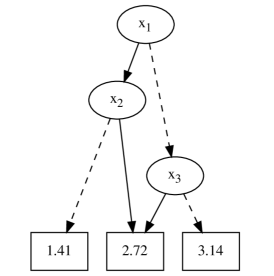
Figure 2: An ADD representing a PB function. If an edge from an oval node is solid (respectively dashed), then the corresponding variable is assigned $1$ (respectively $0$).

5 Evaluation

We conducted computational experiments to answer the following empirical questions.

1. Does DPO significantly contribute to a portfolio of state-of-the-art exact solvers on application benchmarks that are encoded as CNF formulas?

2. Is there a class of XOR-CNF benchmarks on which DPO outperforms existing tools?

We used a high-performance computing cluster. Each solver-benchmark pair was exclusively run on a single core of an Intel Xeon CPU (E5-2650 v2 at 2.60GHz) with a RAM cap of 25 GB and a time cap of 1000 seconds.

Source code, benchmarks, and experimental data are available in a public repository:

https://github.com/vuphan314/DPO

5.1 Solvers

We are aware of only one native Boolean MPE solver [Sang et al., 2007], but its code is no longer available, according to the authors. Fortunately, Boolean MPE can be reduced to weighted partial MaxSAT as described in section 2. The only existing XOR-CNF MaxSAT solver we know is GaussMaxHS [Soos and Meel, 2021].

We also considered the top three solvers in the complete weighted track of the MaxSAT Evaluation 2021: CASHWMaxSAT [Lei et al., 2021], MaxHS [Davies and Bacchus, 2011], and UWrMaxSat [Piotrow, 2020]. But we had to exclude CASHWMaxSAT because it did not report numeric optimal costs; we contacted the authors and are waiting for their response. So we compared three MaxSAT solvers, MaxHS, UWrMaxSat, and GaussMaxHS, to our Boolean MPE tool, DPO. Since MaxHS and UWrMaxSat only work on pure CNF, we employed the Tseitin transformation on benchmarks in XOR-CNF. MaxSAT instances were created before MaxSAT solvers were run, so the MaxSAT reduction time and CNF encoding time were excluded from the total solving time.

5.2 Benchmarks

We used CryptoMiniSat [Soos et al., 2009] to guarantee that every instance is satisfiable. The first benchmark suite comprises 1049 literal-weighted CNF instances that were derived from Bayesian networks [Sang et al., 2005]. The second suite was generated by us. Adapting a recent study on MaxSAT [Kyrillidis et al., 2022], we created random chain formulas in XOR-CNF that have low-width project-join trees. For given integers $n$ and $k$, a chain formula is a conjunction of $n-k+1$ clauses. Clause $i$ involves $k$ variables: $x_{i},x_{i+1},\ldots,x_{i+k-1}$. Each clause is randomly an XOR or a disjunction of literals. The polarity of each literal is also uniformly randomized. Each variable $x$ has random weights: $W_{x}\left(\langle x,0\rangle\right)=10$ and $W_{x}\left(\langle x,1\rangle\right)=100$, or vice versa. For such a formula, there is a simple (left-deep) project-join tree with width $k$. We generated 441 chain benchmarks with $n=100,110,\ldots,300$ and $k=10,11,\ldots,30$. Recall that DPO and GaussMaxHS natively handle XOR-CNF. Since neither MaxHS nor UWrMaxSat accepts XOR, we employed the Tseitin transformation to obtain pure-CNF benchmarks, using PyEDA [Drake, 2015].

5.3 Performance

On the Bayesian benchmark suite, MaxHS performed very well, solving all 1049 instances. DPO only solved 1014 and was faster than MaxHS on three of these benchmarks. There was no need to run UWrMaxSat or GaussMaxHS. The answer to the first empirical question is clear: on these application benchmarks, DPO did not significantly contribute to the state of the art.

On the random chain formulas in XOR-CNF, DPO outperformed MaxHS, UWrMaxSat, and GaussMaxHS. An advantage GaussMaxHS and DPO had was being able to directly process XOR, while MaxHS and UWrMaxSat had to solve larger CNF formulas after the Tseitin transformation. See tables 1 and 3 for more detail on the chain benchmarks.

Table 1: On most of the 441 chain benchmarks, DPO was the fastest solver. VBS0, a virtual best solver, simulates running MaxHS, UWrMaxSat, and GaussMaxHS concurrently and finishing once one of these three actual solvers succeeds. VBS1 simulates the portfolio of MaxHS, UWrMaxSat, GaussMaxHS, and DPO.

Solver	Mean peak RAM (GB)	Benchmarks solved (of 441)			Mean PAR-2 score
		Unique	Fastest	Total
MaxHS	0.10	0	0	441	82.3
UWrMaxSat	0.07	0	12	329	624.8
GaussMaxHS	0.02	0	58	441	6.1
DPO	0.03	0	371	441	1.0
VBS0	NA	NA	NA	441	5.6
VBS1	NA	NA	NA	441	0.3

Figure 3: On this plot, each $\langle x,y\rangle$ point on a solver curve means that the solver would solve $y$ benchmarks in total if the time cap was $x$ seconds per benchmark. DPO was the fastest solver on 371 of 441 chain benchmarks. The improvement of the virtual best solver VBS1 over VBS0 is due to DPO.

Clearly, solvers that only accept pure-CNF benchmarks suffer when there are many hybrid constraints, even with the Tseitin transformation. To answer the second empirical question, we identified a class of XOR-CNF chain formulas on which DPO outperformed state-of-the-art MaxSAT solvers. This class includes hybrid Boolean formulas that have low-width project-join trees.

6 Conclusion

We introduce DPO, a dynamic-programming optimizer that exactly solves Boolean MPE. DPO leverages techniques to build and execute project-join trees from a WMC solver [Dudek et al., 2020]. DPO also adapts an iterative procedure to find maximizers from MaxSAT [Kyrillidis et al., 2022]. Our experiments show that DPO can outperform state-of-the-art MaxSAT solvers (MaxHS [Davies and Bacchus, 2011], UWrMaxSat [Piotrow, 2020], and GaussMaxHS [Soos and Meel, 2021]) by handling XOR-CNF natively and exploiting low-width project-join trees.

For future work, we plan to add support for hybrid inputs, such as PB and cardinality constraints. Also, DPO can be extended to solve more general problems, e.g., existential-random stochastic satisfiability [Lee et al., 2018], maximum model counting [Fremont et al., 2017], and functional aggregate queries [Abo Khamis et al., 2016]. Another research direction is to improve DPO with parallelism, as a portfolio solver (e.g., [Xu et al., 2008]) or with a multi-core ADD package (e.g., [van Dijk and van de Pol, 2015]).

Appendix A Proofs

A.1 Proof of proposition 1

See 1

Proof.

By definition 9 (derivative sign), we have $\left(\operatorname*{dsgn}_{x}f\right)(\tau)=\left\{\langle x,1\rangle\right\}$ if $f(\tau\cup\left\{\langle x,1\rangle\right\})\geq f(\tau\cup\left\{\langle x,0\rangle\right\})$, and $\left(\operatorname*{dsgn}_{x}f\right)(\tau)=\left\{\langle x,0\rangle\right\}$ otherwise. First, assume the former case, $\left(\operatorname*{dsgn}_{x}f\right)(\tau)=\left\{\langle x,1\rangle\right\}$. Then:

$$f\left(\tau\cup\left(\operatorname*{dsgn}_{x}f\right)(\tau)\right) =f\left(\tau\cup\left\{\langle x,1\rangle\right\}\right)$$

$$=\max\left(f\left(\tau\cup\left\{\langle x,0\rangle\right\}\right),f\left(\tau\cup\left\{\langle x,1\rangle\right\}\right)\right)$$ as we assumed the former case

$$=(\exists_{x}f)(\tau)$$ by definition 2 (existential projection)

$$=\left(\exists_{X\setminus\left\{x\right\}}(\exists_{x}f)\right)(\varnothing) \tau \exists_{x}f:\mathbb{B}^{X\setminus\left\{x\right\}}\to\mathbb{R}$$ since is a maximizer of

$$=\left(\exists_{X}f\right)(\varnothing)$$ because existential projection is commutative

So $\tau\cup\left(\operatorname*{dsgn}_{x}f\right)(\tau)$ is a maximizer of $f:\mathbb{B}^{X}\to\mathbb{R}$ by definition 4 (maximizer). The latter case, $\left(\operatorname*{dsgn}_{x}f\right)(\tau)=\left\{\langle x,0\rangle\right\}$, is similar. ∎

A.2 Proof of proposition 2

See 2

Proof.

We prove that the two outputs of the algorithm are the maximum and a maximizer of $f_{n}$, as requested by the Boolean MPE problem (definition 7).

Regarding the first output ($m$), on algorithm 1 of algorithm 1, note that $f_{0}=\exists_{x_{1}}\exists_{x_{2}}\ldots\exists_{x_{n-1}}\exists_{x_{n}}f_{n}=\exists_{X_{n}}f_{n}$. Then $m=f_{0}(\varnothing)=(\exists_{X_{n}}f_{n})(\varnothing)$, which is the maximum of $f_{n}$ by definition 3.

Regarding the second output ($\tau_{n}$), Lines 1-1 of the algorithm iteratively compute each truth assignment $\tau_{i}$ that is a maximizer of the PB function $f_{i}$. This process of iterative maximization is correct due to proposition 1. Finally, $\tau_{n}$ is a maximizer of $f_{n}$. ∎

A.3 Proof of proposition 3

See 3

Proof.

Let $x\in S$ be a variable. We first show that $\Sigma_{x}\left(f\cdot g\right)=\left(\Sigma_{x}f\right)\cdot g:\mathbb{B}^{X\cup Y\setminus\left\{x\right\}}\to\mathbb{R}$. For each truth assignment $\tau:X\cup Y\setminus\left\{x\right\}\to\mathbb{B}$, we have:

$$\left(\Sigma_{x}\left(f\cdot g\right)\right)(\tau)$$

$$=\left(f\cdot g\right)\left(\tau\cup\left\{\langle x,1\rangle\right\}\right)+\left(f\cdot g\right)\left(\tau\cup\left\{\langle x,0\rangle\right\}\right)$$ by definition 5 (additive projection)

$$=f\left(\tau\cup\left\{\langle x,1\rangle\right\}\restriction_{X}\right)\cdot g\left(\tau\cup\left\{\langle x,1\rangle\right\}\restriction_{Y}\right)+f\left(\tau\cup\left\{\langle x,0\rangle\right\}\restriction_{X}\right)\cdot g\left(\tau\cup\left\{\langle x,0\rangle\right\}\restriction_{Y}\right)$$ by definition 1 (join)

$$=f\left(\tau\cup\left\{\langle x,1\rangle\right\}\restriction_{X}\right)\cdot g\left(\tau\restriction_{Y}\right)+f\left(\tau\cup\left\{\langle x,0\rangle\right\}\restriction_{X}\right)\cdot g\left(\tau\restriction_{Y}\right) x\notin Y$$ since

$$=\left(f\left(\tau\cup\left\{\langle x,1\rangle\right\}\restriction_{X}\right)+f\left(\tau\cup\left\{\langle x,0\rangle\right\}\restriction_{X}\right)\right)\cdot g\left(\tau\restriction_{Y}\right)$$ by common factor

$$=\left(f\left(\tau\restriction_{X}\cup\left\{\langle x,1\rangle\right\}\right)+f\left(\tau\restriction_{X}\cup\left\{\langle x,0\rangle\right\}\right)\right)\cdot g\left(\tau\restriction_{Y}\right) x\in X$$ as

$$=\left(\Sigma_{x}f\right)\left(\tau\restriction_{X}\right)\cdot g\left(\tau\restriction_{Y}\right)$$ by definition of additive projection

$$=\left(\Sigma_{x}f\right)\left(\tau\restriction_{X\setminus\left\{x\right\}}\right)\cdot g\left(\tau\restriction_{Y}\right) x\notin\operatorname{dom}\left(\tau\right)=X\cup Y\setminus\left\{x\right\}$$ because

$$=\left(\Sigma_{x}f\cdot g\right)(\tau)$$ by definition of join

Since additive projection is commutative, we can generalize this equality from a single variable $x\in S$ to an equality on a whole set $S$ of variables: $\Sigma_{S}(f\cdot g)=(\Sigma_{S}f)\cdot g$. The case of existential projection, $\exists_{S}(f\cdot g)=(\exists_{S}f)\cdot g$, is similar. ∎

A.4 Proof of theorem 1

See 1

Proof.

This theorem concerns Boolean MPE. A very similar theorem concerns WMC [Dudek et al., 2020, Theorem 2]. We simply adapt that proof [Dudek et al., 2020, Section C.2] and replace additive projection with existential projection. ∎

A.5 Proof of theorem 2

theorem 2 concerns algorithms 2 and 3. We actually prove the correctness of their annotated versions, which are respectively algorithms 4 and 5.

To simplify notations, for a multiset $A$ of PB functions $a$, define $\left[A\right]:=\prod_{a\in A}a$ and $\operatorname{vars}\left(A\right):=\bigcup_{a\in A}\operatorname{vars}\left(a\right)$.

Input: $\varphi$: an XOR-CNF formula

Input: $W$: a literal-weight function over $X=\operatorname{vars}\left(\varphi\right)$

Output: $m\in\mathbb{R}$: the maximum of $\left[\varphi\right]\cdot W$

Output: $\tau\in\mathbb{B}^{X}$: a maximizer of $\left[\varphi\right]\cdot W$

1

2$\mathcal{T}=\langle T,r,\gamma,\pi\rangle\leftarrow$ a project-join tree for $\varphi$

$\sigma\leftarrow\langle\rangle$ // an initially empty stack

$E\leftarrow\varnothing$ // $E\subseteq X$ is a set of variables that have been eliminated via projection

$A\leftarrow\left\{\left[c\right]\mid c\in\varphi\right\}\cup\left\{W_{x}\mid x\in X\right\}$ // $A$ is a multiset of “active” PB functions

${\llbracket r\rrbracket}_{W}\leftarrow\mathtt{Valuator}(\varphi,\mathcal{T},W,r,\sigma,E,A)$ // $\mathtt{Valuator}$ (algorithm 5) modifies $\sigma$, $E$, and $A$

$m\leftarrow{\llbracket r\rrbracket}_{W}(\varnothing)$ // ${\llbracket r\rrbracket}_{W}$ is a constant PB function

$\tau\leftarrow\varnothing$ // an initially empty truth assignment

assert $\tau$ is a maximizer of $\exists_{E}\left(\left[\varphi\right]\cdot W\right)$ // $E=X$ after algorithm 4

3 while $\sigma$ is not empty 

       $d\leftarrow\mathtt{pop}\left(\sigma\right)$ // $d=\operatorname*{dsgn}_{x}f$ is a derivative sign, where $x\in E$ is an unassigned variable and $f$ is a PB function

4       $\tau^{\prime}\leftarrow\tau$

       $\tau\leftarrow\tau^{\prime}\cup d\left(\tau^{\prime}\restriction_{\operatorname{dom}\left(d\right)}\right)$ // $d\left(\tau^{\prime}\restriction_{\operatorname{dom}\left(d\right)}\right)=\left\{\langle x,b\rangle\right\}$, where $b\in\mathbb{B}$

       $E\leftarrow E\setminus\left\{x\right\}$ // $x$ has just been assigned $b$ in $\tau$

5       assert $\tau$ is a maximizer of $\exists_{E}\left(\left[\varphi\right]\cdot W\right)$

6      

7

return $\langle m,\tau\rangle$ // $E=\varnothing$ now (all variables have been assigned in $\tau$)

Algorithm 4 Dynamic Programming for Boolean MPE

Input: $\varphi$: an XOR-CNF formula

Input: $\mathcal{T}=\langle T,r,\gamma,\pi\rangle$: a project-join tree for $\varphi$

Input: $W$: a literal-weight function over $\operatorname{vars}\left(\varphi\right)$

Input: $v\in\mathcal{V}\left(T\right)$: a node

Input: $\sigma$: a stack (of derivative signs) that will be modified

Input: $E$: a set (of variables) that will be modified

Input: $A$: a multiset (of PB functions) that will be modified

Output: ${\llbracket v\rrbracket}_{W}$: the $W$-valuation of $v$

1

assert $\left[A\right]=\exists_{E}\left(\left[\varphi\right]\cdot W\right)$ // pre-condition

2 if $v\in\mathcal{L}\left(T,r\right)$ 

       $f\leftarrow\left[\gamma(v)\right]$ // the Boolean function represented by the clause $\gamma(v)\in\varphi$

3      

4

5else // $v$ is an internal node of $\langle T,r\rangle$

       $f\leftarrow\left\{\langle\varnothing,1\rangle\right\}$ // the PB function for multiplicative identity

6       $A\leftarrow A\cup\left\{f\right\}$

7       for $u\in\mathcal{C}\left(T,r,v\right)$  // non-empty set of nodes

             $h\leftarrow\mathtt{Valuator}(\varphi,\mathcal{T},W,u,\sigma,E,A)$ // recursive call on a child $u$ of $v$

8             $f^{\prime}\leftarrow f$

9             $f\leftarrow f^{\prime}\cdot h$

             $A\leftarrow A\setminus\left\{h\right\}$ // $h$ was added by initialization algorithm 4 of algorithm 4) or a recursive call (algorithm 5 or 5)

             $A\leftarrow A\setminus\left\{f^{\prime}\right\}$ // $f^{\prime}$ was added before this loop (algorithm 5) or in the previous iteration (algorithm 5)

10             $A\leftarrow A\cup\left\{f\right\}$

11            

12      

      assert $\left[A\right]=\exists_{E}\left(\left[\varphi\right]\cdot W\right)$ // join-condition

13       for $x\in\pi(v)$  // possibly empty set of variables

14             $f^{\prime}\leftarrow f$

15             $d\leftarrow\operatorname*{dsgn}_{x}f$

             $\mathtt{push}\left(\sigma,d\right)$ // $\sigma$ will be used to construct a maximizer (algorithm 4)

16             assert $\tau\cup d\left(\tau\restriction_{\operatorname{dom}\left(d\right)}\right)$ is a maximizer of $\exists_{E}\left(\left[\varphi\right]\cdot W\right)$ if $\tau$ is a maximizer of $\exists_{\left\{x\right\}\cup E}\left(\left[\varphi\right]\cdot W\right)$

17             $f\leftarrow\exists_{x}\left(f^{\prime}\cdot W_{x}\right)$

18             $E\leftarrow E\cup\left\{x\right\}$

             $A\leftarrow A\setminus\left\{f^{\prime},W_{x}\right\}$ // $f^{\prime}$ was added before this loop (algorithm 5) or in the previous iteration (algorithm 5); $W_{x}$ was added by initialization algorithm 4 of algorithm 4)

19             $A\leftarrow A\cup\left\{f\right\}$

             assert $\left[A\right]=\exists_{E}\left(\left[\varphi\right]\cdot W\right)$ // project-condition

20            

21      

22      

23

assert $\left[A\right]=\exists_{E}\left(\left[\varphi\right]\cdot W\right)$ // post-condition

return $f$

Algorithm 5 $\mathtt{Valuator}(\varphi,\mathcal{T},W,v,\sigma,E,A)$

Theorem 3 (Correctness of algorithm 4).

Let $\varphi$ be an XOR-CNF formula and $W$ be a literal-weight function over $\operatorname{vars}\left(\varphi\right)$. Then algorithm 4 solves Boolean MPE on $\langle\varphi,W\rangle$.

We will first prove some lemmas regarding algorithm 5.

A.5.1 Proofs for algorithm 5

The following proofs involve an XOR-CNF formula $\varphi$, a project-join tree $\mathcal{T}=\langle T,r,\gamma,\pi\rangle$ for $\varphi$, and a literal-weight function $W$ over $X=\operatorname{vars}\left(\varphi\right)$.

Lemma 2.

The pre-condition of the call $\mathtt{Valuator}(\varphi,\mathcal{T},W,r,\sigma,E,A)$ holds (algorithm 5 of algorithm 5).

Proof.

algorithm 5 is called for the first time on algorithm 4 of algorithm 4. We have:

$$\left[A\right] =\prod_{a\in A}a$$ by definition

$$=\prod_{c\in\varphi}\left[c\right]\cdot\prod_{x\in X}W_{x}$$ as initialized on algorithm 4 of algorithm 4

$$=\prod_{c\in\varphi}\left[c\right]\cdot W W$$ since is a literal-weight function

$$=\left[\varphi\right]\cdot W \varphi$$ because is an XOR-CNF formula

$$=\exists_{\varnothing}\left(\left[\varphi\right]\cdot W\right)$$ by convention

$$=\exists_{E}\left(\left[\varphi\right]\cdot W\right)$$ as initialized on algorithm 4 of algorithm 4

∎

To simplify proofs, for each internal node $v$ of $\mathcal{T}$, assume that the sets $\mathcal{C}\left(T,r,v\right)$ and $\pi(v)$ have arbitrary (but fixed) orders. Then we can refer to members of these two sets as the first, second, …, and last.

Lemma 3.

Let $v$ be an internal node of $\mathcal{T}$ and $u$ be the first node in the set $\mathcal{C}\left(T,r,v\right)$. Note that $\mathtt{Valuator}(\varphi,\mathcal{T},W,v,\sigma,E,A)$ calls $\mathtt{Valuator}(\varphi,\mathcal{T},W,u,\sigma,E,A)$. Assume that the pre-condition of the caller ($v$) holds. Then the pre-condition of the callee ($u$) holds.

Proof.

Before algorithm 5 of algorithm 5, $A$ is modified trivially: inserting the multiplicative identity $f$ does not change $\left[A\right]$. Also, $E$ is not modified. ∎

Lemma 4.

Let $v$ be a leaf of $\mathcal{T}$. Assume that the pre-condition of the call $\mathtt{Valuator}(\varphi,\mathcal{T},W,v,\sigma,E,A)$ holds. Then the post-condition holds (algorithm 5).

Proof.

Neither $A$ nor $E$ is modified in the non-recursive branch of algorithm 5, i.e., when $v\in\mathcal{L}\left(T,r\right)$. ∎

Lemma 5.

Let $v$ be an internal node of $\mathcal{T}$ and $u_{1}<u_{2}$ be consecutive nodes in $\mathcal{C}\left(T,r,v\right)$. Note that $\mathtt{Valuator}(\varphi,\mathcal{T},W,v,\sigma,E,A)$ calls $\mathtt{Valuator}(\varphi,\mathcal{T},W,u_{1},\sigma,E,A)$ then calls $\mathtt{Valuator}(\varphi,\mathcal{T},W,u_{2},\sigma,E,A)$. Assume that the post-condition of the first callee ($u_{1}$) holds. Then the pre-condition of the second callee ($u_{2}$) holds.

Proof.

After the first callee returns and before the second callee starts, $A$ is trivially modified: replacing $h$ and $f^{\prime}$ with $f=f^{\prime}\cdot h$ does not change $\left[A\right]$. Also, $E$ is not modified. ∎

Lemma 6.

Let $v$ be an internal node of $\mathcal{T}$. For each $u\in\mathcal{C}\left(T,r,v\right)$, note that $\mathtt{Valuator}(\varphi,\mathcal{T},W,v,\sigma,E,A)$ calls $\mathtt{Valuator}(\varphi,\mathcal{T},W,u,\sigma,E,A)$. Assume that the post-condition of the last callee holds. Then the join-condition of the caller holds (algorithm 5).

Proof.

After the last callee returns, $A$ is trivially modified: replacing $h$ and $f^{\prime}$ with $f=f^{\prime}\cdot h$ does not change $\left[A\right]$. Also, $E$ is not modified. ∎

Lemma 7.

Let $v$ be an internal node of $\mathcal{T}$ and $x$ be the first variable in $\pi(v)$. Assume that the join-condition of algorithm 5 holds. Then the project-condition holds (algorithm 5).

Proof.

We have:

$$\left[A\right] =\left[\left\{f\right\}\cup A\setminus\left\{f\right\}\right]$$

$$=f\cdot\left[A\setminus\left\{f\right\}\right]$$

$$=\left(\exists_{x}\left(f^{\prime}\cdot W_{x}\right)\right)\cdot\left[A\setminus\left\{f\right\}\right]$$

$$=\exists_{x}\left(f^{\prime}\cdot W_{x}\cdot\left[A\setminus\left\{f\right\}\right]\right) x\notin\operatorname{vars}\left(A\setminus\left\{f\right\}\right) \mathcal{T} W$$ since , as is a project-join tree and is a literal-weight function

$$=\exists_{x}\left[\left\{f^{\prime},W_{x}\right\}\cup A\setminus\left\{f\right\}\right]$$

$$=\exists_{x}\exists_{E\setminus\left\{x\right\}}\left(\left[\varphi\right]\cdot W\right)$$ because the join-condition was assumed to hold

$$=\exists_{E}\left(\left[\varphi\right]\cdot W\right)$$

∎

Lemma 8.

Let $v$ be an internal node of $\mathcal{T}$ and $x_{1}<x_{2}$ be consecutive variables in $\pi(v)$. Assume that the project-condition of algorithm 5 holds in the iteration for $x_{1}$. Then the project-condition also holds in the iteration for $x_{2}$.

Proof.

Similar to lemma 7. ∎

Lemma 9.

Let $v$ be an internal node of $\mathcal{T}$ and $x$ be a variable in $\pi(v)$. Assume that the join-condition of algorithm 5 holds. Then the project-condition holds.

Proof.

Apply lemmas 7 and 8. ∎

Lemma 10.

Let $v$ be an internal node of $\mathcal{T}$. For each $u\in\mathcal{C}\left(T,r,v\right)$, note that $\mathtt{Valuator}(\varphi,\mathcal{T},W,v,\sigma,E,A)$ calls $\mathtt{Valuator}(\varphi,\mathcal{T},W,u,\sigma,E,A)$. Assume that the post-condition of the last callee holds. Then the post-condition of the caller holds.

Proof.

By lemma 6, the join-condition holds. Then by lemma 9, the project-condition holds in the iteration for the last variable in $\pi(v)$. So the post-condition holds. ∎

Lemma 11.

The pre-condition and post-condition of algorithm 5 hold for each input $v\in\mathcal{V}\left(T\right)$.

Proof.

Employ induction on the recursive calls to the algorithm.

In the base case, consider the leftmost nodes of $\mathcal{T}$: $v_{1},v_{2},\ldots,v_{k}$, where $v_{i+1}$ is the first node in $\mathcal{C}\left(T,r,v_{i}\right)$, $v_{1}$ is the root $r$, and $v_{k}$ is a leaf. We show that the pre-condition of the call $\mathtt{Valuator}(\varphi,\mathcal{T},W,v_{i},\sigma,E,A)$ holds for each $i=1,2,\ldots,k$ and that the post-condition of the call $\mathtt{Valuator}(\varphi,\mathcal{T},W,v_{k},\sigma,E,A)$ holds. The pre-condition holds for each $v_{i}$ due to lemmas 2 and 3. The post-condition holds for $v_{k}$ by lemma 4.

In the step case, the induction hypothesis is that the pre-condition holds for each call started before the current call starts and that the post-condition holds for each call returned before the current call starts. We show that the pre-condition and post-condition hold for the current call $\mathtt{Valuator}(\varphi,\mathcal{T},W,v,\sigma,E,A)$. The pre-condition for $v$ holds due to lemmas 3 and 5. The post-condition for $v$ holds by lemmas 4 and 10. ∎

Lemma 12.

The join-condition and project-condition of algorithm 5 hold for each internal node $v$ of $\mathcal{T}$ and variable $x$ in $\pi(v)$.

Proof.

By lemma 11, the post-condition of the last call on algorithm 5 holds. Then by lemma 6, the join-condition holds. And by lemma 9, the project-condition holds. ∎

Lemma 13.

Let $f:\mathbb{B}^{X}\to\mathbb{R}$ and $g:\mathbb{B}^{Y}\to\mathbb{R}$ be PB functions with non-negative ranges. Assume that $x$ is a variable in $X\setminus Y$ and that $\tau$ is a truth assignment for $Y\cup X\setminus\left\{x\right\}$. Then ${\left(\operatorname*{dsgn}_{x}f\right)\left(\tau\restriction_{X\setminus\left\{x\right\}}\right)}=\left(\operatorname*{dsgn}_{x}(f\cdot g)\right)(\tau)$.

Proof.

First, assume the case $\left(\operatorname*{dsgn}_{x}f\right)\left(\tau\restriction_{X\setminus\left\{x\right\}}\right)=\left\{\langle x,1\rangle\right\}$. We have the following inequalities:

$$f\left(\tau\restriction_{X\setminus\left\{x\right\}}\cup\left\{\langle x,1\rangle\right\}\right) \geq f\left(\tau\restriction_{X\setminus\left\{x\right\}}\cup\left\{\langle x,0\rangle\right\}\right)$$ by definition 9 (derivative sign)

$$f\left(\tau\cup\left\{\langle x,1\rangle\right\}\restriction_{X}\right) \geq f\left(\tau\cup\left\{\langle x,0\rangle\right\}\restriction_{X}\right) x\in X$$ as

$$f\left(\tau\cup\left\{\langle x,1\rangle\right\}\restriction_{X}\right)\cdot g\left(\tau\restriction_{Y}\right) \geq f\left(\tau\cup\left\{\langle x,0\rangle\right\}\restriction_{X}\right)\cdot g\left(\tau\restriction_{Y}\right) g$$ because the range of is non-negative

$$f\left(\tau\cup\left\{\langle x,1\rangle\right\}\restriction_{X}\right)\cdot g\left(\tau\cup\left\{\langle x,1\rangle\right\}\restriction_{Y}\right) \geq f\left(\tau\cup\left\{\langle x,0\rangle\right\}\restriction_{X}\right)\cdot g\left(\tau\cup\left\{\langle x,0\rangle\right\}\restriction_{Y}\right) x\notin Y$$ since

$$(f\cdot g)\left(\tau\cup\left\{\langle x,1\rangle\right\}\right) \geq(f\cdot g)\left(\tau\cup\left\{\langle x,0\rangle\right\}\right)$$ by definition 1 (join)

So $\left(\operatorname*{dsgn}_{x}(f\cdot g)\right)(\tau)=\left\{\langle x,1\rangle\right\}$ by definition. Thus ${\left(\operatorname*{dsgn}_{x}f\right)\left(\tau\restriction_{X\setminus\left\{x\right\}}\right)}=\left(\operatorname*{dsgn}_{x}(f\cdot g)\right)(\tau)$. The case $\left(\operatorname*{dsgn}_{x}f\right)\left(\tau\restriction_{X\setminus\left\{x\right\}}\right)=\left\{\langle x,0\rangle\right\}$ is similar. ∎

Lemma 14.

Let $f:\mathbb{B}^{X}\to\mathbb{R}$ and $g:\mathbb{B}^{Y}\to\mathbb{R}$ be PB functions with non-negative ranges. Assume that $x$ is a variable in $X\setminus Y$ and that $\tau$ is a maximizer of $\exists_{x}(f\cdot g)$. Then $\tau^{\prime}=\tau\cup\left(\operatorname*{dsgn}_{x}f\right)\left(\tau\restriction_{X\setminus\left\{x\right\}}\right)$ is a maximizer of $f\cdot g$.

Proof.

By lemma 13, $\tau^{\prime}=\tau\cup\left(\operatorname*{dsgn}_{x}(f\cdot g)\right)(\tau)$. Then by proposition 1 (iterative maximization), $\tau^{\prime}$ is a maximizer of $f\cdot g$. ∎

Lemma 15.

Let $v$ be an internal node of $\mathcal{T}$ and $x$ be a variable in $\pi(v)$. Then the assertion on algorithm 5 of algorithm 5 holds.

Proof.

On that line:

$$\exists_{\left\{x\right\}\cup E}\left(\left[\varphi\right]\cdot W\right) =\exists_{x}\exists_{E}\left(\left[\varphi\right]\cdot W\right)$$

$$=\exists_{x}\left[A\right]$$ as the join-condition and project-condition hold by lemma 12

$$=\exists_{x}\left[\left\{f\right\}\cup A\setminus\left\{f\right\}\right]$$

$$=\exists_{x}\left(f\cdot\left[A\setminus\left\{f\right\}\right]\right)$$

Apply lemma 14. ∎

A.5.2 Proofs for algorithm 4

Lemma 16.

The assertion on algorithm 4 of algorithm 4 holds.

Proof.

algorithm 4 changed $E$ to $X$ after all calls to $\mathtt{Valuator}$ returned. Then $\exists_{E}\left(\left[\varphi\right]\cdot W\right)$ is a constant PB function. So $\tau=\varnothing$ is the maximizer of $\exists_{E}\left(\left[\varphi\right]\cdot W\right)$. ∎

Lemma 17.

Let $d$ be the first derivative sign to be popped in algorithm 4. Then the assertion on algorithm 4 holds at this time.

Proof.

Note that $d=\operatorname*{dsgn}_{x}f$ for some variable $x\in X$ and PB function $f$. Consider the following on algorithm 4. By lemma 16, the truth assignment $\tau^{\prime}$ is a maximizer of $\exists_{\left\{x\right\}\cup E}\left(\left[\varphi\right]\cdot W\right)$. Recall that when $d$ was pushed onto $\sigma$, the assertion on algorithm 5 of algorithm 5 holds (by lemma 15). Then $\tau$ is a maximizer of $\exists_{E}\left(\left[\varphi\right]\cdot W\right)$. ∎

Lemma 18.

Let algorithm 4 successively pop derivative signs $d_{1}$ then $d_{2}$. Assume that the assertion on algorithm 4 holds in the iteration for $d_{1}$. Then the assertion also holds in the iteration for $d_{2}$.

Proof.

Note that $d_{2}=\operatorname*{dsgn}_{x_{2}}f_{2}$ for some variable $x_{2}\in X$ and PB function $f_{2}$. Consider the following on algorithm 4 in the iteration for $d_{2}$. By the assumption, the truth assignment $\tau^{\prime}$ is a maximizer of $\exists_{\left\{x_{2}\right\}\cup E}\left(\left[\varphi\right]\cdot W\right)$. Recall that when $d_{2}$ was pushed onto $\sigma$, the assertion on algorithm 5 of algorithm 5 holds (by lemma 15). Then $\tau$ is a maximizer of $\exists_{E}\left(\left[\varphi\right]\cdot W\right)$. ∎

We are now ready to prove theorem 3.

See 3

Proof.

The first output ($m$) is the maximum of $\left[\varphi\right]\cdot W$ as algorithm 4 computes the $W$-valuation of the root $r$ of a project-join tree for $\varphi$ (see theorem 1 and lemma 1). The second output ($\tau$) is a maximizer of $\left[\varphi\right]\cdot W$ by lemmas 17 and 18. ∎

References

- [Abo Khamis et al., 2016] Abo Khamis, M., Ngo, H. Q., and Rudra, A. (2016). FAQ: questions asked frequently. In PODS.
- [Bacchus et al., 2020] Bacchus, F., Berg, J., Jarvisalo, M., and Martins, R. (2020). MaxSAT Evaluation 2020: solver and benchmark descriptions. Technical report, University of Helsinki.
- [Bahar et al., 1997] Bahar, R. I., Frohm, E. A., Gaona, C. M., Hachtel, G. D., Macii, E., Pardo, A., and Somenzi, F. (1997). Algebraic decision diagrams and their applications. Form Method Syst Des.
- [Bogdanov et al., 2011] Bogdanov, A., Khovratovich, D., and Rechberger, C. (2011). Biclique cryptanalysis of the full AES. In ASIACRYPT.
- [Bryant, 1986] Bryant, R. E. (1986). Graph-based algorithms for Boolean function manipulation. IEEE TC.
- [Cai et al., 2017] Cai, B., Huang, L., and Xie, M. (2017). Bayesian networks in fault diagnosis. IEEE Trans Industr Inform.
- [Charwat and Woltran, 2016] Charwat, G. and Woltran, S. (2016). BDD-based dynamic programming on tree decompositions. Technical report, Technische Universitat Wien.
- [Cook, 1971] Cook, S. A. (1971). The complexity of theorem-proving procedures. In STOC.
- [Costa et al., 2009] Costa, M.-C., de Werra, D., Picouleau, C., and Ries, B. (2009). Graph coloring with cardinality constraints on the neighborhoods. Discrete Optimization.
- [Crama et al., 1990] Crama, Y., Hansen, P., and Jaumard, B. (1990). The basic algorithm for pseudo-Boolean programming revisited. Discrete Applied Mathematics.
- [Davies and Bacchus, 2011] Davies, J. and Bacchus, F. (2011). Solving MaxSAT by solving a sequence of simpler SAT instances. In CP.
- [Drake, 2015] Drake, C. (2015). PyEDA: data structures and algorithms for electronic design automation. In SciPy.
- [Dudek et al., 2020] Dudek, J. M., Phan, V. H., and Vardi, M. Y. (2020). DPMC: weighted model counting by dynamic programming on project-join trees. In CP.
- [Dudek et al., 2021] Dudek, J. M., Phan, V. H., and Vardi, M. Y. (2021). ProCount: weighted projected model counting with graded project-join trees. In SAT.
- [Feldman et al., 2005] Feldman, J., Wainwright, M. J., and Karger, D. R. (2005). Using linear programming to decode binary linear codes. IEEE Transactions on Information Theory.
- [Fichte et al., 2020] Fichte, J. K., Hecher, M., Thier, P., and Woltran, S. (2020). Exploiting database management systems and treewidth for counting. In PADL.
- [Fremont et al., 2017] Fremont, D. J., Rabe, M. N., and Seshia, S. A. (2017). Maximum model counting. In AAAI.
- [Krentel, 1988] Krentel, M. W. (1988). The complexity of optimization problems. Journal of computer and system sciences.
- [Kyrillidis et al., 2020] Kyrillidis, A., Shrivastava, A., Vardi, M., and Zhang, Z. (2020). FourierSAT: a Fourier expansion-based algebraic framework for solving hybrid boolean constraints. In AAAI.
- [Kyrillidis et al., 2022] Kyrillidis, A., Vardi, M. Y., and Zhang, Z. (2022). DPMS: an ADD-based symbolic approach for generalized MaxSAT solving. arXiv preprint arXiv:2205.03747.
- [Lee et al., 2018] Lee, N.-Z., Wang, Y.-S., and Jiang, J.-H. R. (2018). Solving exist-random quantified stochastic Boolean satisfiability via clause selection. In IJCAI.
- [Lei et al., 2021] Lei, Z., Cai, S., Wang, D., Peng, Y., Geng, F., Wan, D., Deng, Y., and Lu, P. (2021). CASHWMaxSAT: solver description. MaxSAT Evaluation 2021.
- [Littman et al., 2001] Littman, M. L., Majercik, S. M., and Pitassi, T. (2001). Stochastic Boolean satisfiability. J Autom Reasoning.
- [Pan and Vardi, 2005] Pan, G. and Vardi, M. Y. (2005). Symbolic techniques in satisfiability solving. J Autom Reasoning.
- [Park, 2002] Park, J. D. (2002). Using weighted MaxSAT engines to solve MPE. In AAAI/IAAI.
- [Pearl, 1985] Pearl, J. (1985). Bayesian networks: a model cf self-activated memory for evidential reasoning. In CogSci.
- [Piotrow, 2020] Piotrow, M. (2020). UWrMaxSat: efficient solver for MaxSAT and pseudo-Boolean problems. In ICTAI.
- [Prestwich, 2009] Prestwich, S. D. (2009). CNF encodings. Handbook of Satisfiability.
- [Robertson and Seymour, 1991] Robertson, N. and Seymour, P. D. (1991). Graph minors. X. Obstructions to tree-decomposition. J Combinatorial Theory B.
- [Saether et al., 2015] Saether, S. H., Telle, J. A., and Vatshelle, M. (2015). Solving# SAT and MaxSAT by dynamic programming. JAIR.
- [Sang et al., 2004] Sang, T., Bacchus, F., Beame, P., Kautz, H. A., and Pitassi, T. (2004). Combining component caching and clause learning for effective model counting. SAT.
- [Sang et al., 2005] Sang, T., Beame, P., and Kautz, H. A. (2005). Performing Bayesian inference by weighted model counting. In AAAI.
- [Sang et al., 2007] Sang, T., Beame, P., and Kautz, H. A. (2007). A dynamic approach for MPE and weighted MaxSAT. In IJCAI.
- [Shwe et al., 1991] Shwe, M. A., Middleton, B., Heckerman, D. E., Henrion, M., Horvitz, E. J., Lehmann, H. P., and Cooper, G. F. (1991). Probabilistic diagnosis using a reformulation of the INTERNIST-1/QMR knowledge base. Methods of information in Medicine.
- [Somenzi, 2015] Somenzi, F. (2015). CUDD: CU decision diagram package–release 3.0.0.
- [Soos et al., 2020] Soos, M., Gocht, S., and Meel, K. S. (2020). Tinted, detached, and lazy CNF-XOR solving and its applications to counting and sampling. In CAV.
- [Soos and Meel, 2019] Soos, M. and Meel, K. S. (2019). BIRD: engineering an efficient CNF-XOR SAT solver and its applications to approximate model counting. In AAAI.
- [Soos and Meel, 2021] Soos, M. and Meel, K. S. (2021). Gaussian elimination meets Maximum Satisfiability. In KRR.
- [Soos et al., 2009] Soos, M., Nohl, K., and Castelluccia, C. (2009). Extending SAT solvers to cryptographic problems. In SAT.
- [Strasser, 2017] Strasser, B. (2017). Computing tree decompositions with FlowCutter: PACE 2017 submission. arXiv preprint arXiv:1709.08949.
- [Tseitin, 1983] Tseitin, G. S. (1983). On the complexity of derivation in propositional calculus. In Automation of reasoning.
- [Valiant, 1979] Valiant, L. G. (1979). The complexity of enumeration and reliability problems. SICOMP.
- [van Dijk and van de Pol, 2015] van Dijk, T. and van de Pol, J. (2015). Sylvan: multi-core decision diagrams. In TACAS.
- [Xu et al., 2008] Xu, L., Hutter, F., Hoos, H. H., and Leyton-Brown, K. (2008). SATzilla: portfolio-based algorithm selection for SAT. JAIR.
- [Yang and Meel, 2021] Yang, J. and Meel, K. S. (2021). Engineering an Efficient PB-XOR Solver. In CP.