Solving optimal control of rigid-body dynamics with collisions using the hybrid minimum principle

Abstract

Collisions are common in many dynamical systems with real applications. They can be formulated as hybrid dynamical systems with discontinuities automatically triggered when states transverse certain manifolds. We present an algorithm for the optimal control problem of such hybrid dynamical systems based on solving the equations derived from the hybrid minimum principle (HMP). The algorithm is an iterative scheme following the spirit of the method of successive approximations (MSA), and it is robust to undesired collisions observed in the initial guesses. We analyze the discontinuities in the system and propose a stable collision condition, which is crucial for the convergence of iterative algorithms in systems experiencing collisions. Subsequently, we establish a convergence theorem demonstrating linear convergence for the MSA algorithm when collisions are present. We also address several numerical challenges introduced by the discontinuities. The algorithm is tested on disc collision problems whose optimal solutions exhibit one or multiple collisions. Linear convergence in terms of iteration steps and asymptotic first-order accuracy in terms of time discretization are observed when the algorithm is implemented with the forward-Euler scheme. The numerical results demonstrate that the proposed algorithm has better accuracy and convergence than direct methods based on gradient descent. Furthermore, the algorithm is also simpler, more accurate, and more stable than a deep reinforcement learning method.

1 Introduction

Discontinuities are ubiquitous in dynamical systems governing many applications, e.g. robotics. They can happen either internally as an intrinsic property of the dynamical system or be triggered by external control signals. These mostly smooth systems with the presence of discrete discontinuous phenomena are called hybrid systems. They can be classified according to the different kinds of hybrid phenomena present in the system [8, 9].

In this paper, we study the optimal control of dynamical systems with discrete discontinuities and a Bolza-type objective. Our interest lies in those discontinuities that are jumps of the state variables and are triggered automatically when the states transverse certain manifolds (jumping manifolds). These discontinuities are called autonomous state jumps. Rigid body collisions are models for these discontinuities, which are very common in robotics.

Another type of hybrid dynamical system that is widely studied in the literature is called controlled hybrid system, i.e. when and how the discontinuities affect the system are directly controlled by extra control variables. Such hybrid phenomena are found in many applications, such as impulsive control of satellite rendezvous [10], Chua’s circuit [22], and hybrid vehicle [28, 7]. Most strategies for solving the optimal control problem of the hybrid system decouple the continuous control and the discrete control, including the switching times, switching sequence, jump magnitudes, etc. For a comprehensive review that focuses on controlled hybrid dynamics, we refer the readers to [7] and the references therein.

However, in systems with autonomous state jumps, these hybrid phenomena are tightly linked to the continuous control; thus, it is difficult to decouple the continuous control and the discrete phenomena. Compared with controlled hybrid systems, autonomous state jumps introduce extra nonlinearity into the problem due to the undetermined times and states at jumps. Furthermore, the total cost may change dramatically when the updated control triggers a new collision or avoids an existing collision in the solution process. These are all challenging issues for optimization.

Dynamic programming and trajectory optimization are two basic approaches for solving optimal control problems. Dynamic programming provides a global optimal closed-loop control based on Bellman’s principle of optimality [6]. It suffers from the curse of dimensionality and generally does not scale to high dimensional systems. Trajectory optimization solves for a locally optimal trajectory and usually provides an open-loop solution. Some methods lie in between, including differential dynamical programming (DDP) [27], iterative linear-quadratic regulator (iLQR) [31], sequential linear-quadratic control (SLQ) [48], and iterative linear-quadratic-Gaussian method (iLQG) [58]. These methods use linear or quadratic approximations around the nominal trajectory for the dynamics or costs to find a local closed-loop control. Since these methods require derivatives of the dynamics, some smoothing techniques that sacrifice accuracy are necessary for their applications in discontinuous systems [56, 35].

In this paper, we will tackle the discontinuous model directly and find the open-loop optimal control. There are two main categories of approaches for the open-loop optimal control problems: direct and indirect methods. Direct methods turn the infinite-dimensional control problems into finite-dimensional nonlinear programming problems through discretization; thus, they are often described as discretize-then-optimize. Being hybrid introduces extra difficulties. For example, the control problem of a frictional system is turned into a mixed-integer programming problem [18]. In [51], it is pointed out that the discretize-then-optimize approach may lead to incorrect gradients. Recently, differentiable physics simulation [23, 61] has also been investigated for solving open-loop optimal control problems involving discontinuities brought by contacts. However, accurately computing the associated gradients remains a challenge that calls for further research efforts [60]. In [5, 4], gradient-type algorithms are proposed for the autonomous hybrid systems where the adjoint equations are used to compute the gradients (with respect to the controls). In this approach, the discontinuity information is implicitly reflected in the gradients and thus influences the continuous controls when applying iterative gradient-based algorithms. Indirect methods use necessary conditions for the optimality of the control problem; they are often described as optimize-then-discretize. They turn the optimal control problem into a system of differential-algebraic equations. The necessary conditions are formulated for the continuous-time problem; thus, they have less to do with how the dynamical system is discretized. Pontryagin’s minimum principle (PMP) [43] is a well-known set of first-order necessary conditions in optimal control. Based on the hybrid maximum principle, an extension of PMP to the hybrid dynamical system, [46] proposed a numerical algorithm (HMP-MAS, short for hybrid maximum principle multiple autonomous switchings) that handles the discontinuities explicitly. For a (estimated) given number of switches and an initial guess of switching times and states, HMP-MAS alternates between computing the optimal controls inside each continuous interval and updating switching times and states by gradient descent. The constraints that switching states must be on the switching manifolds are enforced through the penalty method. This method was proposed for the switching system but can be extended to the state-jump system; see Section 5.5.

This paper proposes an iterative method for the open-loop optimal control of dynamical systems with autonomous state jumps (collisions). We begin with a hybrid minimum principle (HMP) which extends the PMP to the hybrid dynamical systems with autonomous state jumps. We analyze the discontinuity in the system and propose a stable collision condition that is crucial for the convergence of iterative algorithms in systems experiencing collisions. A convergence theorem demonstrating linear convergence is then proven for the method of successive approximation (MSA) algorithm [15]. To the best of our knowledge, this is the first convergence theory for the discontinuous systems considered in this paper. Following HMP and the MSA algorithm, we propose a modified version that incorporates a relaxation technique to improve the convergence. The algorithm automatically avoids unnecessary collisions and does not require an accurate prediction of the number of collision times. It generally converges faster and produces more accurate solutions than gradient-based algorithms. We implement the algorithm with the forward-Euler scheme and numerically address several difficulties introduced by the discontinuities of the hybrid system. The method is tested on disc collision problems with one or multiple collisions. It exhibits stable linear convergence in terms of the iteration steps. Asymptotic first-order accuracy is observed for the $L^{2}$ error on model problems with exact analytic solutions.

This article is organized as follows. In Section 2, we formulate the dynamical systems. The hybrid minimum principle is presented in Section 3. Section 4 presents a convergence theorem for the vanilla MSA algorithm, along with an analysis of the stability of collision. We introduce an HMP-based numerical algorithm and take into account several numerical issues. We demonstrate the performance of the proposed algorithm for several examples in Section 5. Comparisons to the HMP-MAS, a direct method, and a deep reinforcement learning method are then discussed. Finally, we conclude in Section 6 with some discussions on possible extensions.

1.1 Notations

We will denote the state of the system by $\bm{x}(\cdot)\in\mathbb{R}^{m}$ and the control by $\bm{u}(\cdot)\in U\subset\mathbb{R}^{m_{u}}$. The time interval considered is always $[0,T]$. We use $|\bm{z}|$ to denote the Euclidean norm for any $\bm{z}$ in the Euclidean space. For a scalar function $h=h(\bm{z}):\mathbb{R}^{n}\rightarrow\mathbb{R}$, its derivative with respect to $\bm{z}$ is a row vector $\partial_{z}h=h_{z}=[h_{z_{1}},\cdots,h_{z_{n}}]$. For a vector-valued function $\bm{h}=[h_{1},\cdots,h_{k}]^{T}:\mathbb{R}^{n}\rightarrow\mathbb{R}^{k}$, its Jacobian is defined as

$$\bm{h}_{z}=\begin{bmatrix}\partial z_{1}h_{1}&\cdots&\partial z_{n}h_{1}\\ \partial z_{1}h_{2}&\cdots&\partial z_{n}h_{2}\\ \vdots&\ddots&\vdots\\ \partial z_{1}h_{k}&\cdots&\partial z_{n}h_{k}\\ \end{bmatrix}\in\mathbb{R}^{k\times n}.$$

In two dimensions, we also use $x$ and $y$ as subscripts to denote the $x$ and $y$ coordinates, respectively. We define the $L^{p}$ norm for any vector-valued functions $\bm{h}\in L^{p}(a,b;\mathbb{R}^{k})$ as

$$\|\bm{h}\|_{L^{p}(a,b)}=(\int_{a}^{b}|\bm{h}(t)|^{p}~{}dt)^{\frac{1}{p}}.$$ (1)

When $p=\infty$, $\|\bm{h}\|_{L^{\infty}(a,b)}=\||\bm{h}|\|_{L^{\infty}(a,b)}$. When $(a,b)=(0,T)$, we also write $\|\bm{h}\|_{p}=\|\bm{h}\|_{L^{p}(0,T)}$.

2 Problem formulation

Given the initial condition $\bm{x}(0)=\bm{x}_{0}$ and the control process $\bm{u}(t)$, the evolution of state $\bm{x}(t)$ is governed by piecewise smooth dynamics:

$$\dot{\bm{x}}(t)=\bm{f}(\bm{x}(t),\bm{u}(t)),t\in(\gamma_{i},\gamma_{i+1}),i=0,\cdots,M,$$ (2)

where $0=\gamma_{0}<\gamma_{1}<\cdots<\gamma_{M}<\gamma_{M+1}=T$. For each $i=1,\cdots,M$, a jump function $g$ is applied to the state at time $\gamma_{i}$,

$$\bm{x}(\gamma_{i}^{+})=\bm{g}(\bm{x}(\gamma_{i}^{-})).$$ (3)

Here $\bm{x}(\gamma_{i}^{\pm})$ denote the value of $\bm{x}$ at $\gamma_{i}$ evaluated from the right/left time interval, i.e., $\lim_{t\in(\gamma_{i},\gamma_{i+1}),t\rightarrow\gamma_{i}}\bm{x}(t)$ / $\lim_{t\in(\gamma_{i-1},\gamma_{i}),t\rightarrow\gamma_{i}}\bm{x}(t)$, respectively.

Note that the number of jumps $M$ and the jump time $\gamma_{i}$ are not prescribed; instead, they are functions of the control $\bm{u}$. They are determined by a “collision detection” function $\psi(\bm{x})\geq 0$ that checks whether a jump of state occurs. Namely,

$$\psi(\bm{x}(\gamma_{i}^{-}))=0,$$ (4)

and $\psi(\bm{x}(\cdot))>0$ at $\gamma_{i}^{+}$ and all $t$ other than $\gamma_{i}^{-}$. That is why we call such jumps as autonomous state jumps. We assume both $\psi$ and $\bm{g}$ are smooth in an open set containing $\{\bm{x}:\psi(\bm{x})=0\}$.

The optimal control problem is then formulated as

$$\mathmakebox[\widthof{$\underset{\displaystyle\bm{u}(\cdot)}{\mathrm{subject~{}to}}$}][l]{\underset{\displaystyle\bm{u}(\cdot)}{\mathrm{minimize}}}\quad J(\bm{u}(\cdot))=\phi(\bm{x}(T))+\sum_{i=0}^{M}\int_{\gamma_{i}}^{\gamma_{i+1}}L(\bm{x}(t),\bm{u}(t))\,dt,$$ (5a)

$$\mathmakebox[\widthof{$\underset{\displaystyle\phantom{\bm{u}(\cdot)}}{\mathrm{subject~{}to}}$}][c]{{\mathrm{subject~{}to}}}\quad \text{\lx@cref{creftypeplural~refnum}{eq:forward_state}, \lx@cref{refnum}{eq:forward_jump} and~\lx@cref{refnum}{eq:forward_collision}}.$$ (5b)

Here, $\phi$ is the terminal cost function, and $L$ is the running cost function; both are smooth. We assume that $\bm{f},\phi,L$ are time-independent and that $\bm{f},L$ do not switch across different intervals $(\gamma_{i},\gamma_{i+1})$ in this paper for the simplicity of notations. The considered minimum principle and proposed numerical algorithm can work for time-dependent problems and switching systems straightforwardly. See also e.g. [36] for theory for systems with autonomous jumps and switchings.

To ensure that the above model is well-posed, we shall require that the trajectory of the state $\bm{x}$ transverses the manifold $\{\psi=0\}$ where jumps of the state take place. That is, the state $\bm{x}$ should not move tangentially on the manifold, or

$$0\neq\frac{d}{dt}\psi(\bm{x}(t))=\psi_{x}(\bm{x}(t))\dot{\bm{x}}(t)=[\psi_{x}\bm{f}]|_{t}.$$ (6)

Here $\psi_{x}$ is the normal vector for the manifold and $\dot{\bm{x}}=\bm{f}$ is the instantaneous moving direction of the state $\bm{x}$. In the context of collisional rigid body dynamics, $\psi_{x}\bm{f}$ is the relative velocity projected to the contact normal vector, which should be nonzero for the collision to take place. See Section 5 for a concrete example.

3 Hybrid minimum principle

Pontryagin’s maximum principle for standard optimal control can be extended to the discontinuous dynamics introduced here. We shall call this extension the hybrid minimum principle (HMP). To begin with, we introduce the Hamiltonian $H:\mathbb{R}^{m}\times\mathbb{R}^{m}\times U\rightarrow\mathbb{R}$

$$H(\bm{x},\bm{\lambda},\bm{u})=\bm{\lambda}^{T}\bm{f}(\bm{x},\bm{u})+L(\bm{x},\bm{u}).$$ (7)

Theorem 1 (Hybrid Minimum Principle).

Let $\{\bm{x}(t),\bm{u}(t)\}$ be the optimal solution associated with (5), then there exists a costate process $\bm{\lambda}(t):[0,T]\rightarrow\mathbb{R}^{m}$ that satisfies

$$\dot{\bm{\lambda}}(t)=-H_{x}^{T}(\bm{x}(t),\bm{\lambda}(t),\bm{u}(t)),\quad t\in(\gamma_{i},\gamma_{i+1}),\;i=0,\cdots,M,$$ (8)

with the terminal condition

$$\bm{\lambda}(T)=\phi^{T}_{x}(\bm{x}(T)),$$ (9)

and backward jump conditions, $i=1,\cdots,M,$

$$\bm{\lambda}^{T}(\gamma_{i}^{-})=\bm{\lambda}^{T}(\gamma_{i}^{+})\bm{g}_{x}(x(\gamma_{i}^{-}))+\eta_{i}\psi_{x}(\bm{x}(\gamma_{i}^{-})),$$ (10)

where $\eta_{i}\in\mathbb{R}$ satisfies the following equation (variation of collision time)

$$\bm{\lambda}^{T}(\gamma_{i}^{+})\bm{g}_{x}(\bm{x}(\gamma_{i}^{-}))\bm{f}|_{\gamma_{i}^{-}}-\bm{\lambda}^{T}(\gamma_{i}^{+})\bm{f}|_{\gamma_{i}^{+}}+\eta_{i}\psi_{x}(\bm{x}(\gamma_{i}^{-}))\bm{f}|_{\gamma_{i}^{-}}+L|_{\gamma_{i}^{-}}-L|_{\gamma_{i}^{+}}=0.$$ (11)

Here, $h|_{s^{\pm}}$ denotes function $h$ evaluated at $s$ as limits from right and left, respectively. In addition, the optimal control $\bm{u}$ minimizes the Hamiltonian for each $t\in[0,T]$:

$$\bm{u}(t)=\arg\min_{\bm{v}\in U}H(\bm{x}(t),\bm{\lambda}(t),\bm{v}).$$ (12)

We refer to [59] for a proof of this theorem. A few remarks on PMP and HMP are in order.

Remark 1.

By the assumption of transversality eq. 6, we have $\psi_{x}\bm{f}\neq 0$ when $\psi=0$. Therefore the equation eq. 11 is always non-degenerate. We note that the condition eq. 11 from the variation of collision time is equivalent to the Hamiltonian constancy condition quoted in other literature, i.e. $H|_{\gamma_{i}^{-}}=H|_{\gamma_{i}^{+}}$.

Remark 2.

We have omitted the abnormal multiplier in the statement of Theorem 12 for brevity. In a more complete form, there is a technicality involving multiplier $\lambda_{0}\geq 0$ in the Hamiltonian (7) $H=\bm{\lambda}^{T}\bm{f}+\lambda_{0}L$ and in the terminal condition (9) $\bm{\lambda}(T)=\lambda_{0}\phi^{T}_{x}(\bm{x}(T))$. Besides, the $\lambda_{0}$ also presents in front of $L|_{\gamma^{-}_{i}},L|_{\gamma^{+}_{i}}$ in eq. 11, which can be seen from its equivalence to $H|_{\gamma_{i}^{-}}=H|_{\gamma_{i}^{+}}$. In the case where $\lambda_{0}=0$ is the only candidate, the problem is singular and, in some sense, ill-posed [2]. Otherwise, we can rescale the costate $\bm{\lambda}$ so that we can always let $\lambda_{0}=1$ (note that the additional $\eta_{i}$ in eqs. 10 and 11 does not prevent $\bm{\lambda}$ from rescaling). We shall only consider this case and take $\lambda_{0}=1$ in this paper.

Remark 3.

Most proofs of PMP and HMP resort to the calculus of variations with some special classes of control variations. We note that, $H_{u}$ can be interpreted as the Fréchet derivative of the reduced total cost $\hat{J}$ with respect to control function $\bm{u}$ in $L^{2}$, where

$$\hat{J}(\bm{u}(\cdot))=\phi(\bm{x}(T;\bm{u}(\cdot))+\sum_{i=0}^{M}\int_{\gamma_{i}}^{\gamma_{i+1}}L(\bm{x}(t;\bm{u}(\cdot)),\bm{u}(t))\,dt,$$

and $\bm{x}(t;\bm{u}(\cdot))$ denotes the trajectory obtained with control $\bm{u}(\cdot)$ according to eqs. 2, 3 and 4. This argument and its proof is often a step in the complete proof of the PMP and HMP. For a formal derivation, see Chapter 6.2 of [57]. For a rigorous proof, see the proof of necessary conditions of optimality in Chapter 1.4 [26] on continuous dynamics and see those proof of the HMP (e.g. [59]) for the present case.

Remark 4.

The PMP/HMP is related to the Karush-Kuhn-Tucker (KKT) conditions for constrained optimization problems. In fact, the dynamic equations of $\bm{x}$ (eqs. 2, 3 and 4) can be viewed as an infinite-dimensional constraint. The costate $\bm{\lambda}$ plays the role of a continuous-time analogy of the Lagrange multiplier. The HMP/PMP is stronger than the KKT conditions in the sense that it asserts that $H$ is not only stationary but also minimized at the optimal control (eq. 12). Like KKT, the PMP/HMP is only a set of necessary conditions. However, these sets of necessary conditions are often sufficient to provide a good (even optimal) solution given a reasonable initial guess.

Remark 5.

HMP has been studied extensively in the literature. In [52, 21], HMP has been formulated and proved for a general framework of the hybrid dynamic systems. The HMP is proved by reducing the optimal control problem of the hybrid system to the canonical Pontryagin type in [17]. Adding pathwise inequality constraints to the control problem will append related complementary equations to the resulting HMP [13]. In [3], the HMP has been derived for autonomous hybrid dynamical systems whose jump magnitudes are additional control variables. The HMP has also been extended to manifolds where the costate is a trajectory on the cotangent bundle [55].

4 Algorithm

In this section, based on the HMP in Equation 12, we review the MSA algorithm and develop an analysis of the stability of collision and a convergence theorem demonstrating linear convergence for the MSA algorithm. Following the spirit of the MSA algorithm, we develop an improved version for better numerical convergence.

Prior to the development of numerical algorithms, the jump function of the costate requires extra clarification. Equations (10) and (11) are condensed into a jump function $G$ for simplicity as follows:

$$\bm{\lambda}(\gamma_{i}^{-})=\bm{G}(\bm{\lambda}(\gamma_{i}^{+}),\bm{x}(\gamma_{i}^{+}),\bm{x}(\gamma_{i}^{-}),\bm{u}(\gamma_{i}^{+}),\bm{u}(\gamma_{i}^{-})).$$ (13)

Note that $G$ depends on $\bm{x}(\gamma_{i}^{+})$, $\bm{u}(\gamma_{i}^{+})$, and $\bm{u}(\gamma_{i}^{-})$, due to $\eta$. Here $\bm{u}(\gamma_{i}^{\pm})$ refers to the after/before-jump values of $\bm{u}$. To clarify the semantic meaning of the after/before-jump values, we introduce $\beta_{i}$, which denotes the $i$-th discontinuous point of $\bm{u}$. For the optimal solution, we have $\gamma_{i}=\beta_{i}$. Suggested by Theorem 4, when $\bm{u}$ is close to optimal, the number of $\beta_{i}$ equals that of $\gamma_{i}$, i.e. $\bm{x}$ and $\bm{u}$ have the same number of discontinuities; but the location of the discontinuities might be different, i.e. $\gamma_{i}\neq\beta_{i}$. It implies that $\bm{u}(\gamma_{i}^{\pm})$ is not a stable quantity; it might change discontinuously when $\gamma_{i}$ leaps over $\beta_{i}$. We shall use $\bm{u}(\beta_{i}^{\pm})$ instead in designing numerical algorithms. This is also reflected later in eq. 28 for approximating $\beta_{i}$. Therefore, we rewrite equation (13) as

$$\bm{\lambda}(\gamma_{i}^{-})=\bm{G}(\bm{\lambda}(\gamma_{i}^{+}),\bm{x}(\gamma_{i}^{+}),\bm{x}(\gamma_{i}^{-}),\bm{u}(\beta_{i}^{+}),\bm{u}(\beta_{i}^{-})).$$ (14)

Next, we will review the MSA algorithm and develop a modified version using the formula (14) instead.

At a high level, given a control, the forward equations (2) to (4) for the state $\bm{x}(\cdot)$ and the backward equations (8), (9) and (14) for the costate $\bm{\lambda}(\cdot)$ are satisfied by solving the corresponding forward and backward problems, respectively. It remains to find the optimal control $\bm{u}(\cdot)$ such that (12) is also satisfied. To this end, we propose an iterative method. In the $k$-th iteration, given the control $\bm{u}^{k}(\cdot)$, we compute $\bm{x}^{k}(\cdot),\bm{\lambda}^{k}(\cdot)$ by solving the forward and backward dynamics, respectively. We then update the control using the information from minimizing the Hamiltonian (12). To be specific, we define the minimizer $\bm{u}_{*}^{k+1}(\cdot)$ in the $k$-th iteration by

$$\bm{u}_{*}^{k+1}(t)=\arg\min_{\bm{v}\in U}H(\bm{x}^{k}(t),\bm{\lambda}^{k}(t),\bm{v}),\quad\forall t\in[0,T].$$ (15)

If we update $\bm{u}^{k+1}=\bm{u}^{k+1}_{*}$, we arrive at the method of successive approximations (MSA) [15], see Algorithm 1 below. We will provide a convergence analysis of this algorithm under certain conditions discussed in Section 4.1. To enhance the applicability and robustness of the algorithm in numerical computation, we introduce a relaxed version to update $\bm{u}^{k+1}$ (see (22)) in Section 4.2.

4.1 Convergence of the MSA algorithm

We will show that the following vanilla MSA iteration stated in Algorithm 1 is convergent under certain conditions.

Algorithm 1 Vanilla MSA for solving the optimal control with hybrid dynamics

Input the initial guess of the control $\bm{u}^{0}(\cdot)$

for $k=0,1,\cdots$ do

     Plug $\bm{u}^{k}(\cdot)$ into the forward equations (2) to (4) to get the state $\bm{x}^{k}(\cdot)$

     Plug $\bm{u}^{k}(\cdot)$ and $\bm{x}^{k}(\cdot)$ into the backward equations (8), (9) and (14) to get the costate $\bm{\lambda}^{k}(\cdot)$

     Update the control by $\bm{u}^{k+1}(t)=\arg\min_{\bm{v}\in U}H(\bm{x}^{k}(t),\bm{\lambda}^{k}(t),\bm{v})$

end for

We begin with some standard assumptions.

Assumption 1 (Boundedness of control).

We assume $U$, the set of admissible control values, is bounded. Specifically, we assume $|\bm{u}|\leq M_{u}$ for all $\bm{u}\in U$.

Assumption 2 (Optimal solution).

We assume there is an optimal solution $(\bm{x}^{*},\bm{u}^{*},\bm{\lambda}^{*})$ satisfying Equation 12. We also assume there exists only one collision for the optimal solution at $t=\gamma^{*}$.

Throughout this section, we always assume that there is only one collision for simplicity. Theorems with more than one collision can be derived similarly.

Assumption 3 (Smoothness).

We assume Lipschitz continuity on $\bm{f},\bm{g},\psi,L$,

$$|\bm{f}(\bm{x}^{\prime},\bm{u}^{\prime})-\bm{f}(\bm{x},\bm{u})| \leq B_{f,x}|\bm{x}^{\prime}-\bm{x}|+B_{f,u}|\bm{u}^{\prime}-\bm{u}|,$$

$$|\bm{g}(\bm{x}^{\prime})-\bm{g}(\bm{x})| \leq B_{g}|\bm{x}^{\prime}-\bm{x}|,$$

$$|\psi(\bm{x}^{\prime})-\psi(\bm{x})| \leq B_{\psi}|\bm{x}^{\prime}-\bm{x}|,$$

$$|L(\bm{x}^{\prime},\bm{u}^{\prime})-L(\bm{x},\bm{u})| \leq B_{L,x}|\bm{x}^{\prime}-\bm{x}|+B_{L,u}|\bm{u}^{\prime}-\bm{u}|,$$

and partial derivatives $\bm{f}_{x},\bm{g}_{x},\psi_{x},\phi_{x}$,

$$|\bm{f}_{x}(\bm{x}^{\prime},\bm{u}^{\prime})-\bm{f}_{x}(\bm{x},\bm{u})| \leq B_{f_{x}}(|\bm{x}^{\prime}-\bm{x}|+|\bm{u}^{\prime}-\bm{u}|),$$

$$|\bm{g}_{x}(\bm{x}^{\prime})-\bm{g}_{x}(\bm{x})| \leq B_{g_{x}}|\bm{x}^{\prime}-\bm{x}|,$$

$$|\psi_{x}(\bm{x}^{\prime})-\psi_{x}(\bm{x})| \leq B_{\psi_{x}}|\bm{x}^{\prime}-\bm{x}|,$$

$$|\phi_{x}(\bm{x}^{\prime})-\phi_{x}(\bm{x})| \leq B_{\phi_{x}}|\bm{x}^{\prime}-\bm{x}|.$$

Besides, we also assume that $L$ is continuously differentiable in $\bm{x}$.

We shall note that to have local convergence, we need the Lipschitz continuity only in a region near the optimal trajectory. In addition, for functions $\psi,\bm{g},\bm{g}_{x},$ we only need this property in a small region containing the collision manifold.

Assumption 4 (Smooth manifold).

$\psi$ is second-order continuously differentiable in a region containing the level-set $\psi=0$. Assume $|\psi_{x}(\bm{x})|=1$ if $\psi(\bm{x})=0$ for simplicity.

The unit length assumption is only for notational simplicity. In the optimal control problem described in Section 2, $\psi$ is introduced only to define the collision manifold, whose concrete values are unimportant.

Collisions (discontinuities) are unique features of the optimal control problem studied in this paper. For a convergent algorithm, it is crucial that the collisions are stable, i.e. small perturbation in control should not lead to the vanishment of an existing collision, emergence of a new collision, or large variation of the collision time. To be specific, we have the following definition.

Definition 2 (Stability of collision).

Let $\bm{u}_{1}\in(L^{1}\cap L^{\infty})(0,T;U)$ be a control that has only one collision. Denote its collision time as $\gamma_{1}$. We say $\bm{u}_{1}$ has a stable collision if there exists $C_{3},C_{4}$ such that for any $\bm{u}_{2}\in(L^{1}\cap L^{\infty})(0,T;U)$, if

$$\|\bm{u}_{1}-\bm{u}_{2}\|_{1}\leq C_{3},$$

then $\bm{u}_{2}$ also admits exactly one collision at $\gamma_{2}$ with estimate

$$|\gamma_{1}-\gamma_{2}|\leq C_{4}\|\bm{u}_{2}-\bm{u}_{1}\|_{1}.$$

The stability of collision might be hard to verify. We then propose the following strong collision condition, which is sufficient for ensuring stability (Theorem 4).

Definition 3 (Strong collision).

Let $\bm{u}$ be a control whose state $\bm{x}$ has only one collision at $\gamma$. We say $\bm{u}$ has a strong collision if there exists $a>0$, $b>0$, $K>0,S>0$ such that

$$\begin{split}\psi(\bm{x}(t))&\geq\begin{cases}b,\quad&t<\gamma-\frac{b}{K}\\ K(\gamma-t),\quad&\gamma-\frac{b}{K}\leq t<\gamma\\ a,\quad&t>\gamma\end{cases}\\ K&\geq B_{f,u}M_{J}(\bm{u})+S,\end{split}$$ (16)

where $M_{J}(\bm{u})$ is the magnitude of variation at the collision time $t=\gamma$

$$M_{J}(\bm{u})=\sup_{s\in[0,T]}|\bm{u}(\gamma^{-})-\bm{u}(s)|.$$ (17)

Remark 6.

The strong collisiondefined above is not solely a property of the open-loop control $\bm{u}$ itself. It is defined through the state trajectory $\bm{x}$ it controls. Therefore, it also depends on the optimal control problem (such as the initial state $\bm{x}_{0}$).

As we will explain in more details in Appendix B.1, the condition eq. 16 in $t\in[\gamma-b/K,\gamma)$ is essentially equivalent to

$$\left.\frac{d}{dt}\right|_{t=\gamma^{-}}\psi(\bm{x}(t))\leq-K\leq-(B_{f,u}M_{J}(\bm{u})+S).$$

Namely, the collision tendency or the magnitude of velocity projected to the collision normal (i.e. $|\dot{\bm{x}}\cdot\psi_{x}|$) must be strictly larger than the greatest possible variation in dynamics due to perturbations in $\bm{u}$, by a safety margin of $S$. We note that it is stronger than the transversality or solvability condition discussed previously; see Remark 1. The condition eq. 16 in other regions (i.e. $t<b/K$ or $t>\gamma$) guarantees that there will be no new collision after a small perturbation.

Theorem 4 (Stability of collision).

Let $\bm{u}_{1}\in(L^{1}\cap L^{\infty})(0,T;U)$ be a control that has only one collision. Assume it has a strong collision with factors $a,b,K,S$ according to Definition 3, then $\bm{u}_{1}$ has a stable collision according to Definition 2.

Proof.

See Appendix B.4. ∎

Assumption 5 (Stability of collisions).

The optimal control $\bm{u}^{*}$ satisfies the strong collision condition defined in Definition 3.

We also need Lipschitz regularity of the Hamiltonian minimizer:

Assumption 6 (Hamiltonian minimizer).

The Hamiltonian minimizer

$$h(\bm{x},\bm{\lambda})=\arg\min_{\bm{v}\in U}H(\bm{x},\bm{\lambda},\bm{v}),$$ (18)

is differentiable and Lipschitz, i.e.

$$|h(\bm{x}^{\prime},\bm{\lambda}^{\prime})-h(\bm{x},\bm{\lambda})|\leq B_{h}(|\bm{x}^{\prime}-\bm{x}|+|\bm{\lambda}-\bm{\lambda}^{\prime}|)$$ (19)

for some constant $B_{h}$.

With Theorems 4 and 5, any control $\bm{u}$ that is close to $\bm{u}^{*}$ will not lead to a large perturbation of the dynamical system even with the discontinuous phenomenon; specifically, the resulting dynamical system also only has one collision as $\bm{u}^{*}$ does. Additionally, the smoothness of solutions produced by the vanilla MSA algorithm is guaranteed by Assumption 6. We can thus limit our considerations to piecewise smooth functions with two pieces. To measure the distance between such functions, we introduce a semimetric $\mathfrak{d}(\cdot,\cdot)$ as follows:

$$\mathfrak{d}(\bm{v}_{1},\bm{v}_{2})=\max\{\|\bm{v}_{1}-\bm{v}_{2}\|_{L^{\infty}(0,\min\{\beta_{1},\beta_{2}\})},\|\bm{v}_{1}-\bm{v}_{2}\|_{L^{\infty}(\max\{\beta_{1},\beta_{2}\},T)},|\beta_{1}-\beta_{2}|\},$$ (20)

where functions $\bm{v}_{1},\bm{v}_{2}$ are piecewise smooth with only one discontinuity at $\beta_{1},\beta_{2}$, respectively. We put these strictly and prove a contraction property of the vanilla MSA iterations in Theorem 5, which directly leads to a convergence theorem (Theorem 6).

Theorem 5.

Under Assumptions 1, 2, 3, 4, 5 and 6, there are constants $C_{0},C_{0}^{\prime},C_{1}$ such that for any fixed $k\geq 0$, let $\{\bm{u}^{0},\cdots,\bm{u}^{k+1}\}$ generated by the vanilla MSA (Algorithm 1), if

1. the initial guess $\bm{u}^{0}$ that is discontinuous at $\beta^{0}$ and smooth elsewhere satisfies

   $$\mathfrak{d}(\bm{u}^{0},\bm{u}^{*})\leq\frac{K}{C_{0}^{\prime}+\max\{\|\dot{\bm{u}}^{0}\|_{L^{\infty}(0,\beta^{0})},\|\dot{\bm{u}}^{0}\|_{L^{\infty}(\beta^{0},T)}\}}$$ (21)

   where $K$ is the strong collision factor of $\bm{u}^{*}$, and,

2. for $i\leq k$, $\bm{u}^{i}$ is piecewise smooth with only one discontinuity and

   $$\mathfrak{d}(\bm{u}^{i},\bm{u}^{*})\leq C_{0}$$

then $\bm{u}^{k+1}$ is also piecewise smooth with only one discontinuity and

$$\mathfrak{d}(\bm{u}^{k+1},\bm{u}^{*})\leq C_{1}\mathfrak{d}(\bm{u}^{k},\bm{u}^{*}).$$

Proof.

See Appendix B.7. ∎

Theorem 6 (Convergence of MSA).

Under Assumptions 1, 2, 3, 4, 5 and 6, let the optimal control problem has $C_{1}<1$ (from Theorem 5) and the initial guess $\bm{u}^{0}$ satisfies eq. 21, then the vanilla MSA (Algorithm 1) converges linearly in the semimetric $\mathfrak{d}(\cdot,\cdot)$:

$$\frac{\mathfrak{d}(\bm{u}^{k+1},\bm{u}^{*})}{\mathfrak{d}(\bm{u}^{k},\bm{u}^{*})}\leq C_{1}<1.$$

There are many possibilities for $C_{1}<1$. For details, see the proofs and Remark 7 in Appendix B. One such example is the weakly controlled system given by

$$\dot{\bm{x}}=\bm{f}_{0}(\bm{x})+\delta\bm{f}_{1}(\bm{x},\bm{u}),$$

where $\delta>0$ is small. See Example 1 in Appendix B for a concrete example.

4.2 The relaxed MSA algorithm

The convergence theorem 6 imposes demanding requirements on both the optimal control problem and the initial guess. In fact, even for optimal control problems without discontinuities, the MSA method only converges for a restricted class of linear systems [1]. One reason is that the control $\bm{u}_{*}^{k+1}$ may stray too far from the region of validity approximated at $\bm{u}^{k}$, and the total objective may even increase (see [30] for a more detailed explanation). In [30], an extended version of the method of successive approximations is proposed to penalize the deviations from the dynamic constraints on the state and costate, i.e., $\dot{\bm{x}}^{k}-H_{\lambda}(\bm{x}^{k},\bm{\lambda}^{k},\bm{u}^{k+1})$ and $\dot{\bm{\lambda}}^{k}+H_{x}(\bm{x}^{k},\bm{\lambda}^{k},\bm{u}^{k+1})$. In this paper, we propose to adopt the following update scheme with relaxation:

$$\bm{u}^{k+1}(t)=(1-\alpha)\bm{u}^{k}(t)+\alpha\bm{u}_{*}^{k+1}(t),\quad\forall t\in[0,T]$$ (22)

where $\alpha\in(0,1]$ is a relaxation parameter. Here, we choose to use a small $\alpha$ in eq. 22 to restrict the update of the control.

We now discuss the numerical implementation of the iterative scheme presented above. Each iteration consists of the following four steps.

1. Using the control from the last iteration, we numerically simulate the forward dynamics eqs. 2, 3 and 4 using the forward-Euler scheme with the collision times prediction. The active collision indexes and the states before and after collisions are gathered for the backward dynamics in the simulation.

2. Solve the backward dynamics eqs. 8, 9, 10 and 11 using the forward Euler scheme (backward in time) and the gathered collision information.

3. Update the control pointwise in time according to eqs. 15 and 22 with the newly computed state and costate.

4. Check whether convergence has been achieved.

The whole algorithm is summarized in Algorithm 2. It remains to solve each subprogram in Algorithm 2 with proper time discretization. To this end, we discretize the time interval $[0,T]$ into $N$ uniform intervals: $t_{n}=n\Delta t,$ $n=0,\cdots,N,$ $\Delta t=\frac{T}{N}$. When describing the discretization of the forward and backward dynamics below, we drop the iteration superscript $k$ for simplicity. $\bm{x}_{n},\bm{\lambda}_{n},\bm{u}_{n}$ denote the numerical approximations of the state, costate, and control at $t_{n}$, respectively. Now, we describe each subprogram in detail.

Algorithm 2 The relaxed MSA algorithm for solving optimal control with hybrid dynamics

Input: the number of discretization time intervals $N$, the initial guess of the control $\bm{u}^{0}=[\bm{u}_{0}^{0},\bm{u}_{1}^{0},\cdots,\bm{u}_{N-1}^{0}]$, the convergence criteria $\delta>0$.

$k\leftarrow 0$

while True do

     Program Forward

         

Plug $\bm{u}^{k}$ into eqs. 23 and 24 to get $\bm{x}^{k}=[\bm{x}_{0}^{k},\bm{x}_{1}^{k},\cdots,\bm{x}_{N}^{k}]$, the active collision indexes set $\mathcal{C}$ defined in eq. 25, and the states $\bm{x}_{c+\frac{1}{2}}^{\pm}$ around collision for $c\in\mathcal{C}$.

     

     Program Backward

         

Using computed $\bm{x}^{k}$ and derived information around collisions, obtain $\bm{\lambda}^{k}=[\bm{\lambda}_{1}^{k},\cdots,\bm{\lambda}_{N}^{k}]$ by solving the backward dynamics with jumps described in eqs. 26 and 27. The control values $\bm{u}_{c+\frac{1}{2}}^{\pm}$ in eq. 27 are computed by combining eqs. 28 and 29.

     

     Program Control Update

         

Get control $\bm{u}^{k+1}=[\bm{u}^{k+1}_{0},\cdots,\bm{u}^{k+1}_{N-1}]$ according to eqs. 30 and 31.

     

     Program Convergence Test

         

Compute discrete $L^{2}$ norm of $H_{u}$ according to eq. 35. If it is less than $\delta$, return the control $\bm{u}^{k}$.

     

     $k\leftarrow k+1$  

end while

Output: the optimal control $\bm{u}^{k}$

Forward dynamics

The numerical simulation of a hybrid dynamical system with discontinuities is not a simple task, and there are many related works in the literature [14, 20, 47, 11, 12]. The key idea involves an accurate estimation of the collision time using a root-finding scheme and a proper integration step around the collision by a variable-step integrator. Our integrator estimates the collision time based on a linear approximation and adds an intermediate time step at the estimated time. To be specific, at each step, we estimate the collision time by solving the equation

$$s_{n}=s(\bm{x}_{n},\bm{u}_{n})=\inf\{s>0:\psi(\bm{x}_{n}+s\bm{f}(\bm{x}_{n},\bm{u}_{n}))=0\}.$$ (23)

Here, $s_{n}=\infty$ means the set of solutions is empty, i.e. no collision is predicted from the current state $x_{n}$ with control $u_{n}$. If $s_{n}<\Delta t$, we then insert an extra integration step at $t_{n}+s_{n}$ and apply the jump function $g$ at this step. The forward dynamics is summarized as follows:

$$\begin{cases}\text{If }s_{n}=s(\bm{x}_{n},\bm{u}_{n})<\Delta t,&\begin{cases}\begin{split}\bm{x}_{n+\frac{1}{2}}^{-}&=\bm{x}_{n}+s_{n}\bm{f}(\bm{x}_{n},\bm{u}_{n}),\\ \bm{x}_{n+\frac{1}{2}}^{+}&=\bm{g}(\bm{x}_{n+\frac{1}{2}}^{-}),\\ \bm{x}_{n+1}&=\bm{x}_{n+\frac{1}{2}}^{+}+(\Delta t-s_{n})\bm{f}(\bm{x}_{n+\frac{1}{2}}^{+},\bm{u}_{n+\frac{1}{2}}^{+}),\end{split}\end{cases}\\ \text{If }s_{n}=s(\bm{x}_{n},\bm{u}_{n})\geq\Delta t,\quad&\bm{x}_{n+1}=\bm{x}_{n}+\Delta t\bm{f}(\bm{x}_{n},\bm{u}_{n}),\end{cases}$$ (24)

for $n=0,\cdots,N-1$. Here, $\bm{u}_{n+\frac{1}{2}}^{+}=\bm{u}_{n+1}$ if we only have a discrete sequence of the control. We note that the estimation of the collision time does not add much complexity to the simulation in practice. At most integration steps $t_{n}$ where no collision happens within a time step, a fast but rough estimation of $s_{n}$ is sufficient. This paper focuses on controlling such dynamical systems. Readers interested in convergence may consult [39, 40] for a rigorous analysis of similar dynamics.

After the forward simulation according to (24), we define the active collision index set $\mathcal{C}$ to include those $n$ such that $s_{n}<\Delta t$ in the simulation,

$$\mathcal{C}=\{n:s_{n}<\Delta t\}.$$ (25)

Backward dynamics

The discretization of the backward costate equations (eqs. 8, 9 and 14) is as follows. With the terminal condition $\bm{\lambda}_{N}=\phi_{x}^{T}(\bm{x}_{N},t_{N}),$ for $n=N-1,N-2,\cdots,1$, we have

$$\bm{\lambda}_{n}=\bm{\lambda}_{n+1}+\Delta tH_{x}^{T}(\bm{x}_{n},\bm{\lambda}_{n+1},\bm{u}_{n}),\quad\text{ if }n\notin\mathcal{C},$$ (26)

and if $n\in\mathcal{C}$,

$$\bm{\lambda}_{n+\frac{1}{2}}^{+} =\bm{\lambda}_{n+1}+(\Delta t-s_{n})H_{x}^{T}(\bm{x}_{n+\frac{1}{2}}^{+},\bm{\lambda}_{n+1},\bm{u}_{n+\frac{1}{2}}^{+}),$$ (27a)

$$\bm{\lambda}_{n+\frac{1}{2}}^{-} =\bm{G}(\bm{\lambda}_{n+\frac{1}{2}}^{+},\bm{x}_{n+\frac{1}{2}}^{+},\bm{x}_{n+\frac{1}{2}}^{-},\bm{u}_{n+\frac{1}{2}}^{+},\bm{u}_{n+\frac{1}{2}}^{-})),$$ (27b)

$$\bm{\lambda}_{n} =\bm{\lambda}_{n+\frac{1}{2}}^{-}+s_{n}H_{x}^{T}(\bm{x}_{n},\bm{\lambda}_{n+\frac{1}{2}}^{-},\bm{u}_{n}).$$ (27c)

Here, the function jump function $G$ is defined in eq. 14. In practice, the discontinuities will introduce numerical instability, especially when solving eq. 27b. The absence of $\Delta t$ in eq. 27b means that for $c\in\mathcal{C}$, an error of $O(1)$ in $\bm{u}^{\pm}_{c+\frac{1}{2}}$ will result in an error of $O(1)$ in $\bm{\lambda}_{c}$, and thus in all $\bm{\lambda}_{k}$ for $k\leq c$. This is distinct from eqs. 24 and 26 when the dynamics is continuous and there is always a factor $\Delta t$. Therefore, some extra numerical treatments are needed in order to ensure numerical stability and convergence speed when estimating $\bm{u}_{c+\frac{1}{2}}^{+},\bm{u}_{c+\frac{1}{2}}^{-}$ in evaluating (27). From equation (14), these two values represent the values of the control after and before the collision, respectively. The following two paragraphs are devoted to a better estimation of $\bm{u}_{c+\frac{1}{2}}^{+},\bm{u}_{c+\frac{1}{2}}^{-}$.

Ideally, the discontinuities of the optimal control and collisions should occur simultaneously. However, as addressed in replacing eq. 13 by eq. 14, in the algorithm with time discretization, they can misalign before convergence due to the relaxed updating rule of $\bm{u}$ in eq. 22. During iterations, we observe significant delays in the discontinuities of the control in response to the shifting discontinuities in the state $\bm{x}$. For each $c\in\mathcal{C}$, an inappropriate estimation of $\bm{u}_{c+\frac{1}{2}}^{+},\bm{u}_{c+\frac{1}{2}}^{-}$ will slowdown the convergence and even worse prevent the algorithm from converging. By eq. 14, instead of using the control values $\bm{u}_{c+1},\bm{u}_{c}$ closest to the collision (which can be viewed as a numerical approximation of $\bm{u}(\gamma_{i}^{\pm})$), we propose to use the steepest varying control values near the collision (which can be viewed as a numerical approximation of $\bm{u}(\beta_{i}^{\pm})$). To be specific, we find

$$c^{*}=\arg\max_{|n-c|<l}|\bm{u}_{n}-\bm{u}_{n+1}|,$$ (28)

where $l$ is a given integer. Then $t_{c^{*}}$ can be understood as the numerical resolution of the discontinuous point $\beta_{i}$ of $\bm{u}$. The information around $t_{c^{*}}$ will be used to determine $\bm{u}_{c+\frac{1}{2}}^{+},\bm{u}_{c+\frac{1}{2}}^{-}$, as explained in the next paragraph. In practice, we choose $l=\tau N,\tau\in(0,1)$ so that the range in which we search for the discontinuity is independent of the discretization. Namely, we resolve better control estimations locally in $(t_{c}-\tau T,t_{c}+\tau T)$, where $t_{c}=c\Delta t$. $\tau T$ should be less than the shortest time between adjacent collisions. In our experiments presented in Section 5, we always take $\tau=0.05.$

In the experiments, we also observe that the convergence of the control around collisions is much slower (or even not convergent). This phenomenon is caused by the discontinuities in the control and the fluctuation of simulated collision indexes. To be specific, let us focus on a collision index $c\in\mathcal{C}$. From the forward dynamics eq. 24 and the backward dynamics eq. 27, the state $\bm{x}$ and costate $\bm{\lambda}$ change discontinuously from $c$ to $c+1$ and from $c+1$ to $c$, respectively. Then, the control values $\bm{u}_{c},\bm{u}_{c+1}$ are updated to different values when applying eqs. 30 and 31. If in the next iteration, this collision index shifts from $c$, for example, to $c^{\prime}=c+1$, $\bm{u}_{c^{\prime}}=\bm{u}_{c+1}$ will update to the “before-collison” target. Then, $\bm{u}_{c+1}$ would oscillate between two different values without convergence. In other words, the control values around collisions might approach two distinct targets $\bm{u}^{opt,-},\bm{u}^{opt,+}$ alternatively and thus oscillate between these two targets endlessly, where $\bm{u}^{opt,-},\bm{u}^{opt,+}$ are the optimal controls before/after a collision, respectively. To avoid this oscillation, we should rely on the control values farther from the collisions to make more stable estimations since the controls are continuous in each segment. As the control after/before a collision is right/left continuous, we will use the control values after/before the collision to approximate $\bm{u}_{c+\frac{1}{2}}^{+}/\bm{u}_{c+\frac{1}{2}}^{-}$. To be specific, when estimating $\bm{u}_{c+\frac{1}{2}}^{+},\bm{u}_{c+\frac{1}{2}}^{-}$, instead of using the control values at $c^{*}+1,c^{*}$ from eq. 28, we extrapolate them by the control values in $\mathcal{I}_{j,p}^{+}=\{c^{*}+1+i:i\in\{j,\cdots,p\}\}$ and $\mathcal{I}_{j,p}^{-}=\{c^{*}-i:i\in\{j,\cdots,p\}\}$, respectively, where $p\geq j\geq 1$ are integers. In this paper, we choose the simple approach corresponding to $j=p=1$:

$$\bm{u}_{c+\frac{1}{2}}^{+}=\bm{u}_{c^{*}+2},\quad\bm{u}_{c+\frac{1}{2}}^{-}=\bm{u}_{c^{*}-1}.$$ (29)

We remark that choosing $p$ and the extrapolation scheme depends on the desired order of accuracy and the stability of underlying dynamics, which reflects a trade-off between stability and accuracy. If a higher-order integration scheme is applied to solve the forward and backward dynamics, one should apply a higher-order extrapolation method with $p>j$. Besides, one may take larger $p,j$ if the unstable dynamics brings large fluctuations in the collision times during iterations. We note that other than the accuracy concerns, the distances (in time $t$) to adjacent collisions prohibit selecting large $p$.

Updating the control

It remains to discretize the equation (15). From the discretization of $\bm{x},\bm{\lambda}$ described above, we obtain $\bm{x}_{0}^{k},\cdots,\bm{x}_{N}^{k}$ and $\bm{\lambda}_{1}^{k},\cdots,\bm{\lambda}_{N}^{k}$ in the $k$-th step by using $\bm{u}^{k}$, and we need to update the control at $t_{0},\cdots,t_{N-1}$. Note that the control at $t_{N}=T$ is not used in the discretized forward and backward dynamics; thus, we do not need to update it. For each $\bm{u}_{n}$ to be updated, the costate information should be backpropagated from $\bm{\lambda}_{n+1}$. So we apply the following rule at each time step $n$,

$$\bm{u}_{*,n}^{k+1}=\arg\min_{\bm{v}\in U}H(\bm{x}_{n}^{k},\bm{\lambda}_{n+1}^{k},\bm{v}),\quad n=0,\cdots,N-1.$$ (30)

We then discretize eq. 22 straightforwardly in a pointwise manner:

$$\bm{u}^{k+1}_{n}=(1-\alpha)\bm{u}^{k}_{n}+\alpha\bm{u}_{*,n}^{k+1},\quad n=0,\cdots,N-1.$$ (31)

Equation 30 defines a finite-dimensional optimization problem for each $n$, which can be solved in parallel. In cases like the examples considered in this paper, there are analytical expressions for the minimizers of the Hamiltonian. If $H$ is convex in $\bm{u}$ for fixed $\bm{x},\lambda$, many efficient convex optimization algorithms can be used. Otherwise, a general numerical optimizer can also perform well with the initial guesses from the last iterations and adjacent grids.

We should mention that the above choice of indexes for $\bm{x}$ and $\bm{\lambda}$ at time step $n$ is also consistent with the discretize-then-optimize approach. Namely, consider the following discrete problem without any collision:

$$\mathmakebox[\widthof{$\underset{\displaystyle\bm{u}_{0},\cdots,\bm{u}_{N-1}}{\mathrm{subject~{}to}}$}][l]{\underset{\displaystyle\bm{u}_{0},\cdots,\bm{u}_{N-1}}{\mathrm{minimize}}}\quad\phi(\bm{x}_{N})+\sum_{i=0}^{N-1}L(\bm{x}_{i},\bm{u}_{i})\Delta t,$$ (32a)

$$\mathmakebox[\widthof{$\underset{\displaystyle\phantom{\bm{u}_{0},\cdots,\bm{u}_{N-1}}}{\mathrm{subject~{}to}}$}][c]{{\mathrm{subject~{}to}}}\quad \bm{x}_{n+1}=\bm{x}_{n}+\Delta t\bm{f}(\bm{x}_{n},\bm{u}_{n}).$$ (32b)

If we introduce the Lagrange multiplier $\bm{\lambda}_{n}$ corresponding to the dynamic constraint at each time step and derive the first-order necessary condition, we will have

$$H_{u}(\bm{x}_{*,n},\bm{\lambda}_{*,n+1},\bm{u}_{*,n})=0,$$ (33)

where the subscript $*$ denotes the optimal solution for the discrete problem. We can see that the time indexes in eq. 33 are consistent with those in eq. 30.

Convergence test

Since the forward dynamics of $\bm{x}$ and the backward dynamics of $\bm{\lambda}$ are always solved accurately in the previous steps, we only need to check the Hamiltonian minimization condition eq. 12 to determine if convergence is achieved. The $L^{2}$ norm of $H_{u}$ (eq. 12) serves as a natural convergence indicator. As pointed out in Remark 3, $H_{u}$ also has the meaning of the derivative of the total cost with respect to the control $\bm{u}$. Given $\bm{u}^{k}=[\bm{u}^{k}_{0},\cdots,\bm{u}^{k}_{N-1}]$, $H_{u}$ is discretized as

$$H_{u,n}^{k}=H_{u}(\bm{x}^{k}_{n},\bm{\lambda}^{k}_{n+1},\bm{u}^{k}_{n}),\;n=0,\cdots,N-1.$$ (34)

The indexes relation follows the same logic as in eq. 30. We then compute the numerical $L^{2}$ norm as

$$\sqrt{\sum_{n=0}^{N-1}(H_{u,n}^{k})^{2}\Delta t}.$$ (35)

We stop the algorithm when the above quantity is less than a pre-specified tolerance number $\delta$.

5 Experiments

This paper mainly focuses on those hybrid dynamics whose difficulties are introduced by collisions. We will demonstrate the performance of Algorithm 2 in this scenario by applying it to the rigid body dynamics for a system composed of two-dimensional discs without frictional forces. These discs are homogeneous and fully characterized by their masses and radii. We remove the degrees of freedom associated with the orientations and angular velocities as these quantities are constant in frictionless rigid body dynamics of discs.

There are always two discs in the following experiments. Denote the masses of these two discs by $m_{1},m_{2}$ and the radii by $r_{1},r_{2}$. In this paper, we always take $m_{1}=m_{2}=1,r_{1}=r_{2}=0.2$ and the coefficient of restitution $C_{R}=1$, i.e. perfectly elastic collision. These parameters are summarized in Table 1.

Table 1: Common parameters for all experiments

mass			radius			coefficient of restitution
$m_{1}$	$m_{2}$		$r_{1}$	$r_{2}$		$C_{R}$
1	1		0.2	0.2		1

We control disc 1 by applying a force to it so that it collides with disc 2 in a way that disc 2 will be close to the prescribed locations at the terminal time $T$. Due to the translation invariance, the terminal location is always set to the origin $(0,0)$.

Below we specify the control problem in terms of the equations eqs. 2, 3, 4 and 5. The state $\bm{x}$ is composed of the positions and velocities of the two discs, i.e. $\bm{x}\in\mathbb{R}^{8}.$ Let us write $\bm{x}=[\bm{x}_{q_{1}}^{T},\bm{x}_{q_{2}}^{T},\bm{x}_{v_{1}}^{T},\bm{x}_{v_{2}}^{T}]^{T}$, where $\bm{x}_{q_{i}},\bm{x}_{v_{i}}$ are the position and the velocity of disc $i$, respectively. We similarly write $\bm{\lambda}=[\bm{\lambda}_{q_{1}}^{T},\bm{\lambda}_{q_{2}}^{T},\bm{\lambda}_{v_{1}}^{T},\bm{\lambda}_{v_{2}}^{T}]^{T}$.

The dynamics of two discs

The control $\bm{u}\in\mathbb{R}^{2}$ denotes the force applied to disc 1. The field $\bm{f}$ is

$$\bm{f}(\bm{x},\bm{u})=\begin{pmatrix}0_{4}&I_{4}\\ 0_{4}&0_{4}\end{pmatrix}\bm{x}+\begin{pmatrix}0_{4\times 2}\\ M_{1}^{-1}\\ 0_{2\times 2}\end{pmatrix}\bm{u},$$ (36)

where $I_{4}$ is a $4\times 4$ identity matrix and $M_{1}=\text{diag}(m_{1},m_{1})$ is the inertial matrix. $0_{k}=0_{k\times k},0_{m\times n}$ are zero matrices.

The collision function

The contact normal vector $\mathbf{n}$ is the unit vector in the collision axis

$$\mathbf{n}=\frac{\bm{x}_{q_{1}}-\bm{x}_{q_{2}}}{|\bm{x}_{q_{1}}-\bm{x}_{q_{2}}|}.$$ (37)

We denote $\bm{v}_{1}=\bm{x}_{v_{1}},\bm{v}_{2}=\bm{x}_{v_{2}}$ for simplicity. Let $\bm{v}_{i,E},i=1,2$ be the velocities after (elastic) collision,

$$\bm{v}_{1,E} =\bm{v}_{1}-\frac{2m_{2}(\bm{v}_{1}-\bm{v}_{2})\cdot\mathbf{n}}{m_{1}+m_{2}}\mathbf{n},$$

$$\bm{v}_{2,E} =\bm{v}_{2}+\frac{2m_{1}(\bm{v}_{1}-\bm{v}_{2})\cdot\mathbf{n}}{m_{1}+m_{2}}\mathbf{n}.$$

Then the after collision velocities are,

$$\bm{v}_{1,*} =\bm{v}_{1,E}+(C_{R}-1)(\bm{v}_{1,E}\cdot\mathbf{n})\mathbf{n}-(C_{R}-1)(\bm{v}_{\text{COM}}\cdot\mathbf{n})\mathbf{n},$$ (39a)

$$\bm{v}_{2,*} =\bm{v}_{2,E}+(C_{R}-1)(\bm{v}_{2,E}\cdot\mathbf{n})\mathbf{n}-(C_{R}-1)(\bm{v}_{\text{COM}}\cdot\mathbf{n})\mathbf{n},$$ (39b)

where $C_{R}\in[0,1]$ is the coefficient of restitution and $\bm{v}_{\text{COM}}=(m_{1}\bm{v}_{1}+m_{2}\bm{v}_{2})/(m_{1}+m_{2})$ is the center of mass velocity for the two disc system. The positional components of $\bm{g}$ are kept unchanged. In summary, the collision function $\bm{g}$ is,

$$\bm{g}(\bm{x})=[\bm{x}_{q_{1}}^{T},\bm{x}_{q_{2}}^{T},\bm{v}_{1,*}^{T},\bm{v}_{2,*}^{T}]^{T}.$$ (40)

The collision detection

In the problems considered here, collisions happen when the distance between the two bodies equals 0, and tends to decrease further. The distance between the two discs can be computed by subtracting the sum of their radii from the distance between their centers. The distance will keep decreasing if $(\bm{x}_{q_{1}}-\bm{x}_{q_{2}})\cdot(\bm{x}_{v_{1}}-\bm{x}_{v_{2}})<0$, or equivalently, $\mathbf{n}\cdot(\bm{x}_{v_{1}}-\bm{x}_{v_{2}})<0$, recalling that $\mathbf{n}$ is the contact normal defined in eq. 37. Therefore, we can take

$$\psi(\bm{x})=\frac{\sqrt{2}}{2}\times\begin{cases}|\bm{x}_{q_{1}}-\bm{x}_{q_{2}}|-r_{1}-r_{2}\quad&\text{if }\mathbf{n}\cdot(\bm{x}_{v_{1}}-\bm{x}_{v_{2}})<0\\ 1\quad&\text{elsewhere}\end{cases},$$ (41)

Note that though $\psi$ is not continuous in $\mathbb{R}^{8}$, it is smooth in the following open set of interest with some $0<\xi<r_{1}+r_{2}$

$$\{\bm{x}\in\mathbb{R}^{8}:(\bm{x}_{q_{1}}-\bm{x}_{q_{2}})\cdot(\bm{x}_{v_{1}}-\bm{x}_{v_{2}})<0,|\bm{x}_{q_{1}}-\bm{x}_{q_{2}}|>\xi\}.$$

For $\bm{x}$ in this set,

$$\psi_{x}(\bm{x})=\frac{\sqrt{2}}{2}[\mathbf{n},-\mathbf{n},0_{2},0_{2}],$$

where $0_{2}\in\mathbb{R}^{2}$ is the zero vector. We note that the dot product $\sqrt{2}\psi_{x}\bm{f}=\mathbf{n}\cdot(\bm{x}_{v_{1}}-\bm{x}_{v_{2}})$ is the relative velocity, whose negativity implies that $\eta$ can be solved from eq. 11.

The control objective

The terminal cost term $\phi$ is taken to be the distance between disc 2 and the origin,

$$\phi(\bm{x})=|\bm{x}_{q_{2}}|^{2}.$$ (42)

The running cost function is the square of the Euclidean norm of the applied force in the examples considered in this paper, except for Section 5.4, where the running cost will be prescribed. To be specific, we have

$$L(\bm{x},\bm{u})=\epsilon|\bm{u}|^{2},$$ (43)

where $\epsilon>0$ is a fixed parameter. The space of admissible control values (i.e. $U$) associated with this cost is $\mathbb{R}^{2}$.

The Hamiltonian

The Hamiltonian for the problem (except Section 5.4) is given by

$$H(\bm{x},\bm{\lambda},\bm{u})=\bm{\lambda}_{q_{1}}\cdot\bm{x}_{v_{1}}+\bm{\lambda}_{q_{2}}\cdot\bm{x}_{v_{2}}+\frac{1}{m_{1}}\bm{\lambda}_{v_{1}}\cdot\bm{u}+\epsilon|\bm{u}|^{2}.$$ (44)

Thus, the direct minimizer of $H$ is

$$\bm{u}_{*}=\arg\min_{\bm{v}\in U}H(\bm{x},\bm{\lambda},\bm{v})=-\frac{\bm{\lambda}_{v_{1}}}{2\epsilon},$$ (45)

and $H_{u}$ is

$$H_{u}(\bm{x},\bm{\lambda},\bm{u})=\bm{\lambda}_{v_{1}}+2\epsilon\bm{u}.$$ (46)

Like most iterative algorithms in nonlinear optimal control, a suitable initial guess is necessary to avoid undesired local minima. This is more demanding for the discontinuous systems considered in this paper. For instance, in our disc collision problems, the terminal cost only depends on disc 2, and the control only accelerates disc 1. If the initial control does not trigger a state jump of disc 2, any local optimization algorithm is likely to converge to zero control ($\bm{u}=0$) since the derivative of the total cost with respect to the control $u$ vanishes at zero control (see Remark 3). To avoid this and facilitate the convergence to the global minimum, we choose the initial controls so that all the desired collision pairs (disc 1 and disc 2, disc 2 and wall) will be encountered. Details are provided in each subsection below.

To describe and quantify the performance of the algorithm, we define the $L^{2}$ semi-norm of a square integrable function $l(\cdot):[0,T]\rightarrow\mathbb{R}$ as,

$$||l||_{2}=[\frac{1}{T-2\omega}(\int_{0}^{t_{c}-\omega}l^{2}(t)~{}dt+\int_{t_{c}+\omega}^{T}l^{2}(t)~{}dt)]^{1/2},$$ (47)

when there is only one collision in the optimal trajectory and $t_{c}$ denotes the corresponding collision time. In the integral, we are excluding a small interval with length $2\omega>0$ around the collision time. When there are multiple collisions, the semi-norm can be defined similarly. For a vector-valued function $\bm{h}=[h_{x},h_{y}]^{T}$, we define its $L^{2}$ semi-norm as

$$||\bm{h}||_{2}=(||h_{x}||_{2}^{2}+||h_{y}||_{2}^{2})^{1/2}.$$ (48)

Note that we always use $x,y$ subscripts to denote the $x,y$ coordinates since our experiments are in 2D. In (47) and (48), we abuse the notation of $L^{2}$ norm $\|\cdot\|_{2}$. We will use the definitions here throughout Section 5.

This semi-norm can better measure the distance between the simulated numerical control and the analytical one than the $L^{2}$ norm. The reason is that a tiny shift of the collision time may introduce a relatively large numerical difference in the controls (and the $L^{2}$ norm), which nevertheless has negligible effects on the dynamics. One should take $\omega$ to be larger than the smallest discretization size $\Delta t$. In the experiments, we take $\omega=0.05T$.

In the following experiments, we will always denote the analytical solution for the optimal control by $\bm{u}^{opt}$, the total objective by $J$, and the optimal values of the objective by $J^{opt}$. We will denote the simulated optimal first collision time by $s$ and its analytical solution by $s^{opt}$.

5.1 Concentric collision

We first consider the case when the optimal control is to drive disc 1 to hit disc 2 concentrically. We take the initial state as $\bm{q}_{1}=[-2,-2]^{T},\bm{q}_{2}=[-1,-1]^{T},\bm{v}_{1}=\bm{v}_{2}=[0,0]^{T}$ and $\epsilon=0.1,T=1$. The objective is to push disc 1 to strike disc 2 so that disc 2 will be close to the origin at the terminal time $T=1$. See Figure 1a for an illustration of the setup.

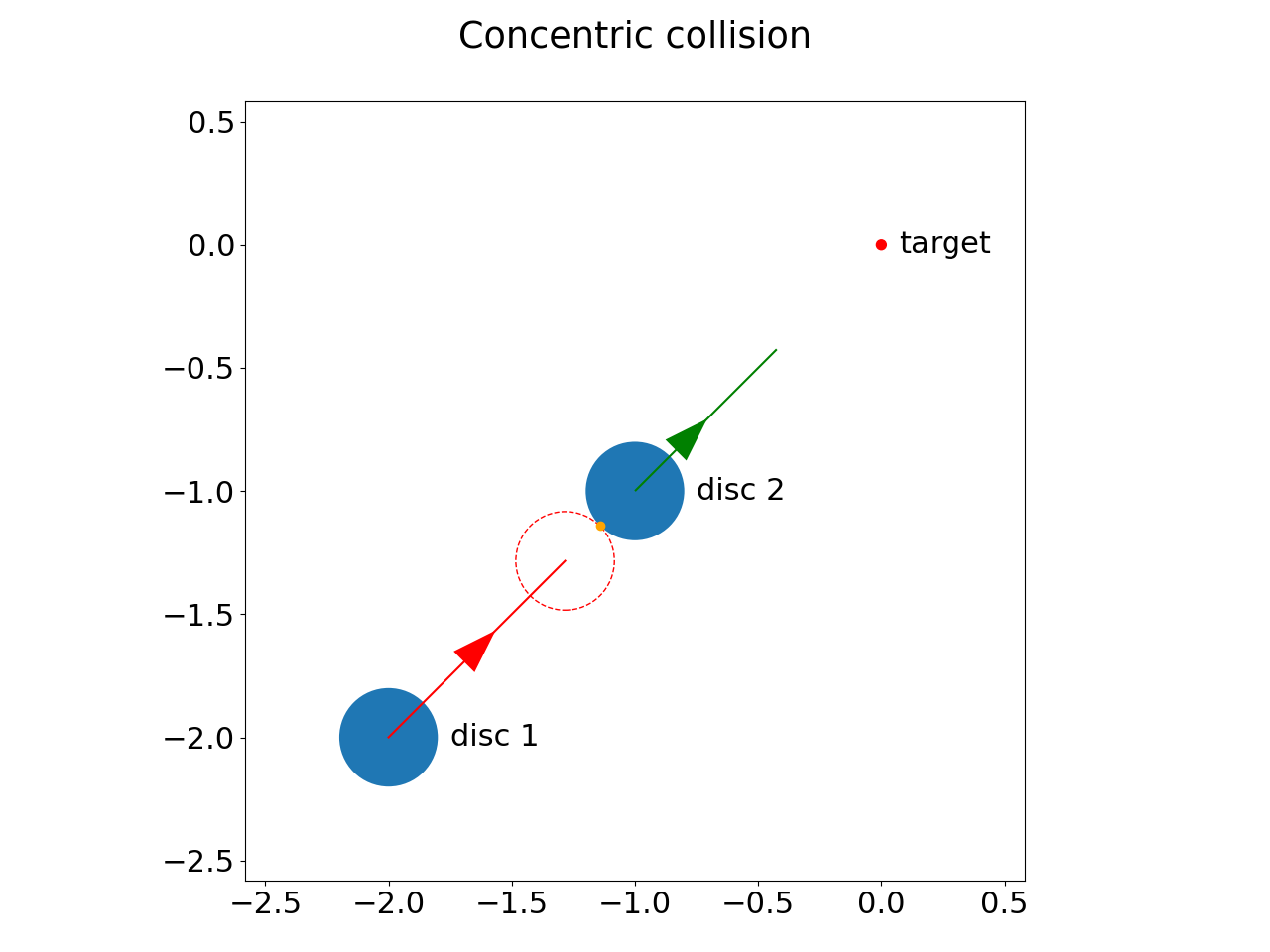
(a) Initial configurations

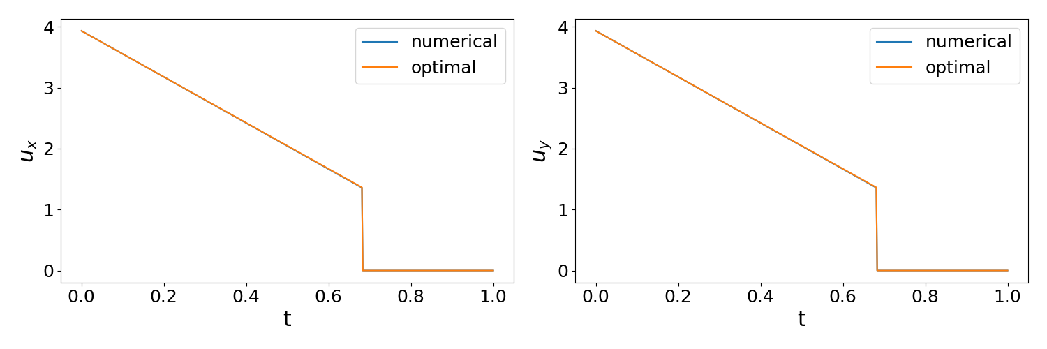
(b) Shape of the optimal control

Fig. 1: Illustration of the concentric collision in Section 5.1. LABEL:sub@fig:case3_illustration Initial state: The initial locations of discs are the blue discs. The red line and green line are optimal trajectories of disc 1 and disc 2, respectively. The dashed red circle is the before-collision position of disc 1. The orange point is the collision point. LABEL:sub@fig:case3_shape The numerical optimal control and the analytical optimal control, $\bm{u}=[u_{x},u_{y}]$.

We discretize the dynamics into 480 steps, i.e. $N=480$ and run Algorithm 2 with the relaxation parameter $\alpha=0.01$. The initial control can be any force fields that make collisions between the two discs happen. Here, we take a constant force $[3,3]^{T}$. The optimal analytical control for this example can be solved to machine accuracy; see Appendix A. See also Figure 1a for the optimal trajectories under the optimal control. We have shown and compared the simulated numerical control and the analytical optimal control, see Figure 1b.

In Figure 2, we visualize the solution process by showing how the cost, $||H_{u}||_{2},$ and $||\bm{u}-\bm{u}^{opt}||_{2}$ converge during the iteration. We can see that the algorithm converges well in a few hundred iterations. Besides, the convergence indicator $||H_{u}||_{2}$ indicates that the algorithm converges linearly for this example.

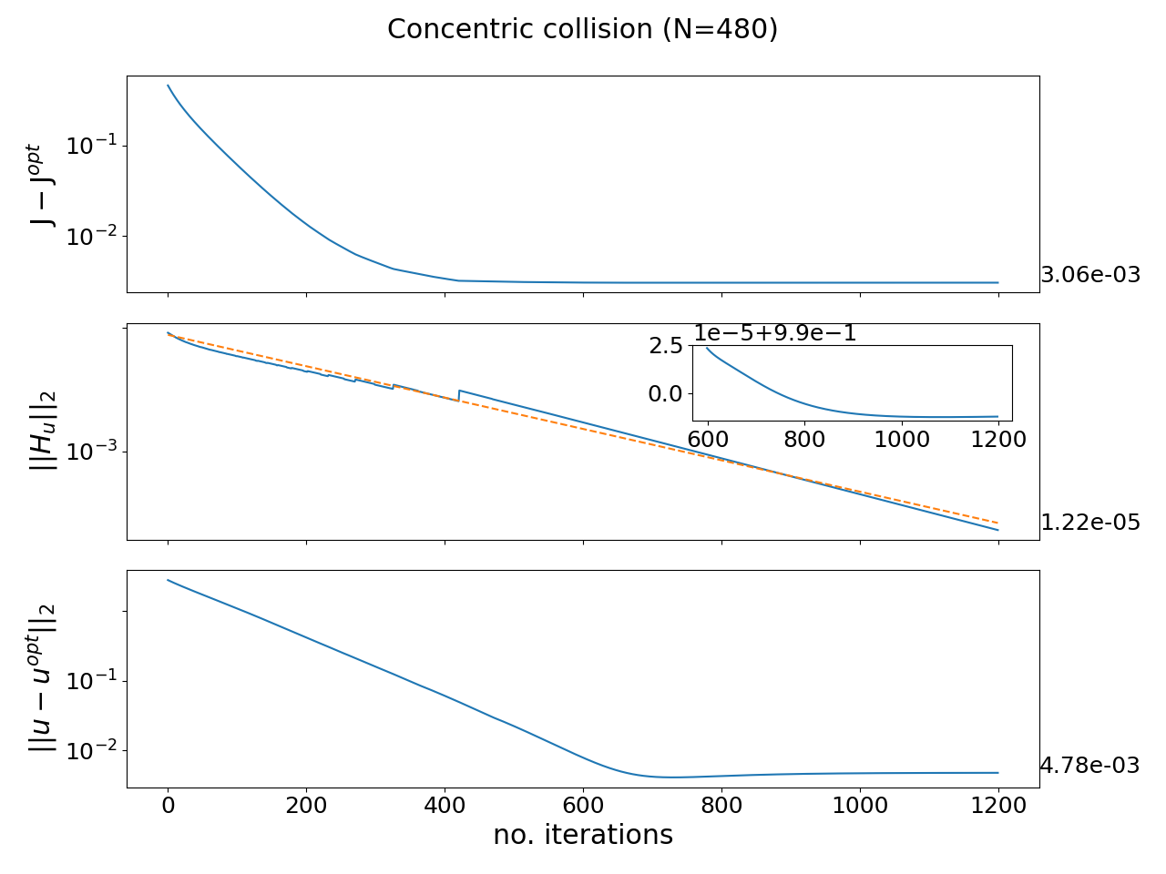
Fig. 2: The example of concentric collision in Section 5.1: the convergence of the iterative algorithm. The annotations on the right are the final values of the corresponding curves. The common $x$ axis denotes the number of iterations spent in the Algorithm 2. Top: the difference between the analytical optimal objective and the numerical solutions. Middle: the $L^{2}$ semi-norm of the derivative of the Hamiltonian with respect to control $\bm{u}$. The dashed line is the result of the regression in the form $\mu\sigma^{k}$ (this is the linear regression after taking the logarithm. $k$ is the number of iterations, $\mu,\sigma$ are positive regression parameters). The inset plot is the ratio $\|H_{u}^{k+1}\|_{2}/\|H_{u}^{k}\|_{2}$ versus the number of iterations. It suggests that the rate of linear convergence is approximately $0.99$. Bottom: the difference between the analytical optimal control and the numerical solutions in terms of the $L^{2}$ semi-norm.

We repeated the experiments for $N=60,120,\cdots,1200.$ We find that the numerical solution for the optimal control converges to the analytical solution, and that the simulated collision times also converge to the analytical solution. Perfect first-order accuracy is observed; see Figure 3.

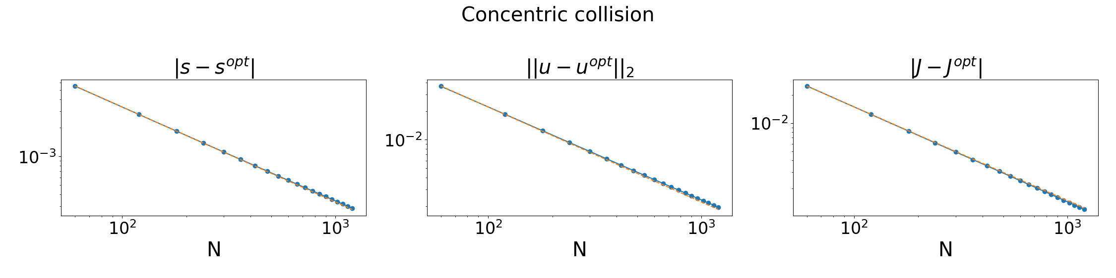
Fig. 3: The example of concentric collision in Section 5.1: convergence to the analytical solution when the number of time intervals $N$ tends to infinity. The dashed orange lines are straight lines obtained from the least square regression on the data with model $\sigma/N$ and parameter $\sigma$. Left: Difference between the simulated collision times and the analytical optimal collision time. Middle: Difference between the numerical and analytical solutions for the optimal controls in terms of the $L^{2}$ semi-norm. Right: Difference between the simulated total costs and the analytical solution.

5.2 General situation for two discs

This experiment shows that our algorithm performs well in more general situations, i.e., when relative velocity forms a non-zero angle with the axis of collision. We take the initial state to be $\bm{q}_{1}=[-1,-2]^{T},\bm{q}_{2}=[-1,-1]^{T},\bm{v}_{1}=\bm{v}_{2}=[0,0]^{T}$ and $\epsilon=0.01,T=1$. See Figure 4a for an illustration of the setup.

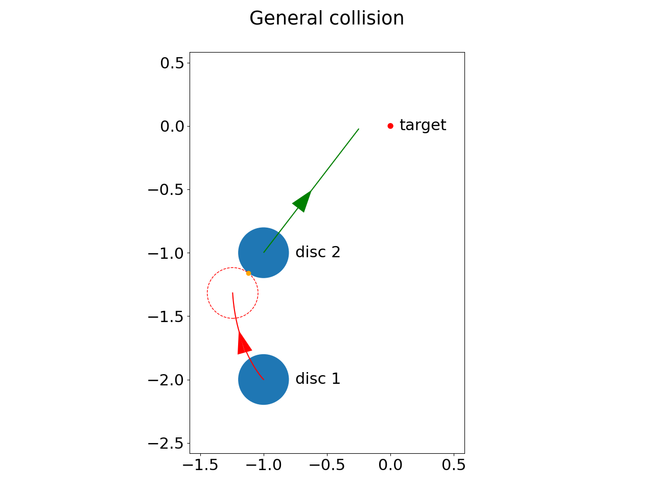
(a) Initial configurations

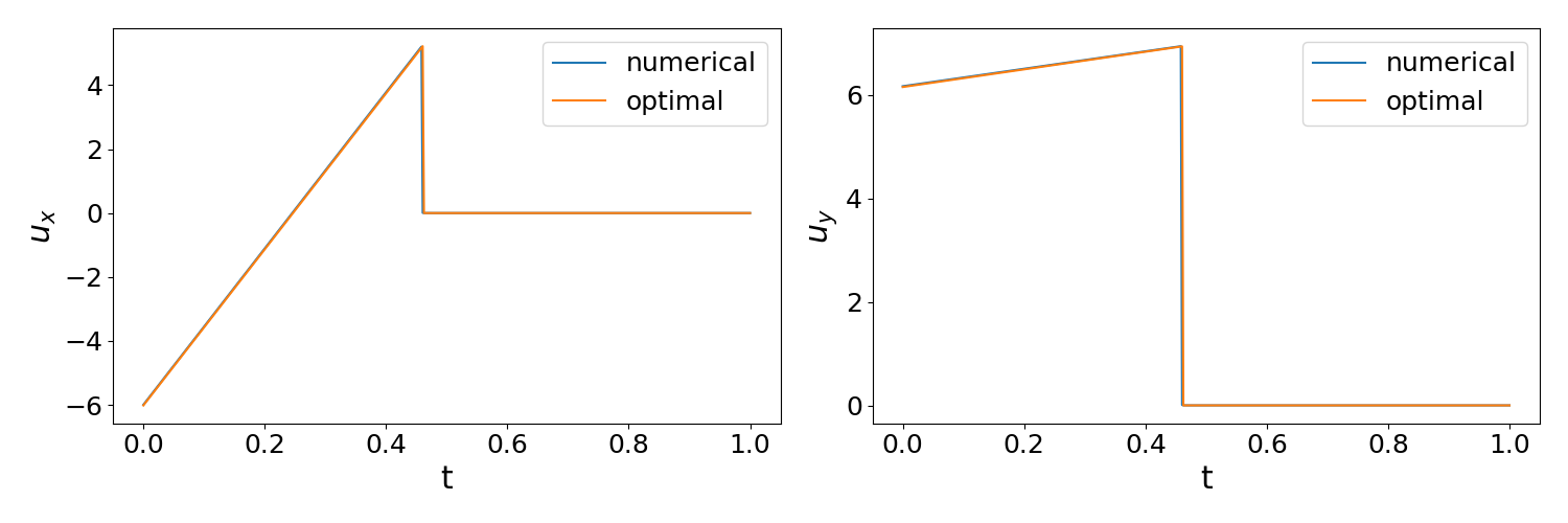
(b) Shape of the optimal control

Fig. 4: Illustration of the general situation of two discs in Section 5.2. LABEL:sub@fig:case3_oblique_illustration Initial state: The initial locations of the discs are the blue discs. The red and green lines are the optimal trajectories of disc 1 and disc 2, respectively. The dashed red circle is the before-collision position of disc 1. The orange point is the collision point. LABEL:sub@fig:case3_oblique_shape The numerical and analytical solutions for the optimal control, $\bm{u}=[u_{x},u_{y}]$.

We discretize the dynamics into 480 steps, i.e. $N=480$ and run Algorithm 2 with the relaxation parameter $\alpha=0.01$. The initial control is a constant field $[0,3]^{T}$ under which disc 1 collides with disc 2. The analytical solution can also be found for this problem, see Appendix A for the derivation and Figure 4a for the optimal trajectories. The numerical result is shown and compared to the analytical one in Figure 4b.

In Figure 5, we show the change of cost, $||H_{u}||_{2}$ and $||\bm{u}-\bm{u}^{opt}||_{2}$. We see that a few hundred iterations are sufficient for convergence. We notice that linear convergence is also observed in terms of the convergence indicator $||H_{u}||_{2}$.

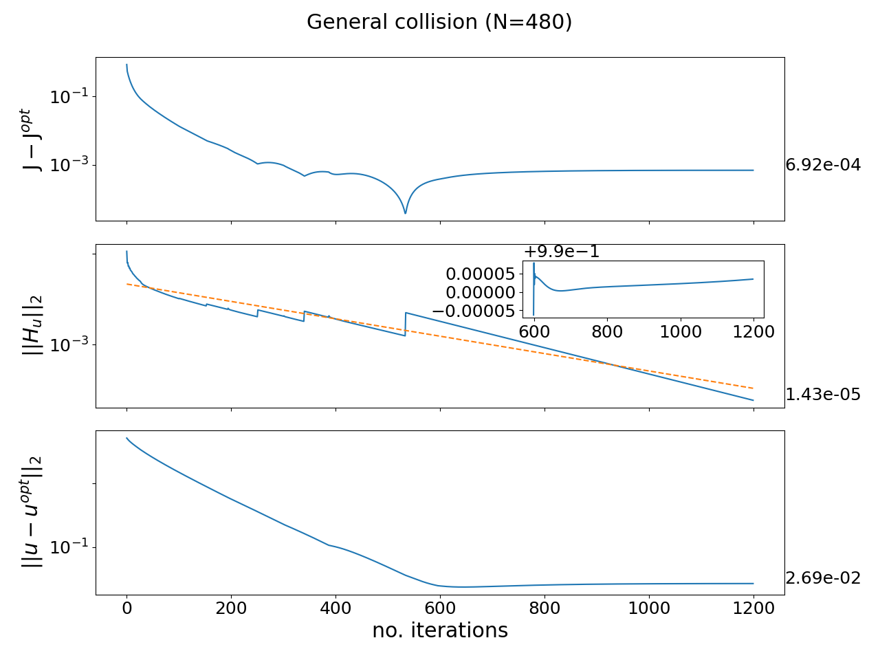
Fig. 5: The example of general situation of two discs in Section 5.2: the convergence of the iterative algorithm. The annotations on the right are the final values of the corresponding curves. The common $x$ axis is the number of iterations spent in Algorithm 2. Top: the difference between the analytical optimal objective and the numerical solutions. Middle: the $L^{2}$ semi-norm of the derivative of the Hamiltonian with respect to the control $\bm{u}$. The dashed line is the result of the regression in the form $\mu\sigma^{k}$ (this is the linear regression after taking the logarithm. $k$ is the number of iterations, $\mu,\sigma$ are positive regression parameters). The inset plot is the ratio $\|H_{u}^{k+1}\|_{2}/\|H_{u}^{k}\|_{2}$ versus number of iterations. Bottom: the difference between the analytical optimal control and the numerical solutions in terms of the $L^{2}$ semi-norm.

We also demonstrate the convergence to the analytical solution as $N$ increases. Asymptotic first-order accuracy is observed for this case; see Figure 6.

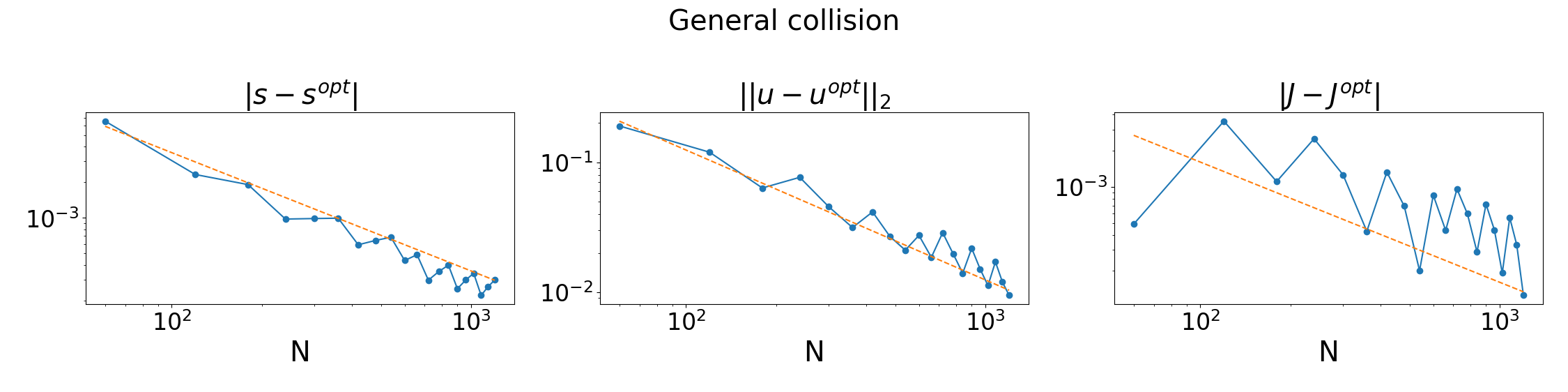
Fig. 6: The example of general situation of two discs in Section 5.2: convergence to the analytical solution when the number of time intervals $N$ tends to infinity. The dashed orange lines are straight lines obtained from the least square regression on the data with model $\sigma/N$ and parameter $\sigma$. Left: Difference between the simulated collision times and the analytical optimal collision time. Middle: Difference between the numerical and analytical solutions for the optimal controls in terms of $L^{2}$ semi-norm. Right: Difference between the simulated total costs and the optimal analytical solution.

5.3 Multiple collisions

In this example, we test our algorithm in the case where multiple collisions are needed to achieve optimality. We add a wall that can be viewed as a rigid body with an infinitely large mass. There are three possible collisions in this system; inter-disc, the wall with disc 1 and the wall with disc 2. A natural way to model this system is to independently model the collision, i.e. the detection and jump functions, of each possible colliding pair of rigid bodies. Let us discuss how we can consolidate these collision models into the formulation presented in Section 2. We shall assume that these collisions are isolated, i.e. at most one collision occurs at a time.

In eq. 4, we assume that $\psi$ is a positive scalar function. In general, one can introduce a vector-valued detection function $\bm{\psi}^{*}=[\psi_{1},\cdots,\psi_{n_{c}}]^{T}:\mathbb{R}^{m}\rightarrow\mathbb{R}^{n_{c}}$, where $n_{c}$ is the number of possible colliding rigid body pairs. Each coordinate $\psi^{*}_{i}$ corresponds to the collision detection of a rigid body pair. There are also $n_{c}$ associated jump functions $\bm{g}^{*}_{1},\cdots,\bm{g}^{*}_{n_{c}}$. We assume $\psi^{*}_{i}$ and $\bm{g}^{*}_{i}$ are smooth.

The vector-valued formulation can be converted to the scalar-valued formulation if collisions are isolated. To be specific, we let $\mathcal{K}_{i}=\{\bm{x}:\psi_{i}^{*}(\bm{x})=0\},i=1,\cdots,n_{c}$ and $B(\bm{x},\delta)$ be the open ball with radius $\delta$ centered at $\bm{x}$. The domain of interest is given by

$$\mathcal{X}=\left\{\bm{x}:\begin{array}[]{cc}\exists\delta>0,\,i\in\{1,\dots,n_{c}\}\text{ such that }\\ B(\bm{x},\delta)\cap\mathcal{K}_{i}\neq\emptyset,B(\bm{x},\delta)\cap\mathcal{K}_{j}=\emptyset\text{ for }j\neq i\end{array}\right\}.$$

One can think of this set as follows. We cover the isolated collision states, the union of all jumping manifolds $\mathcal{K}_{i}$ subtracting their pairwise intersections, by open balls intersecting precisely one of those manifolds. According to the definition, for any $\bm{x}\in\mathcal{X}$, we can define the unique active index $i(\bm{x})$ such that the only possible collision in the neighborhood of $\bm{x}$ is on $\mathcal{K}_{i(\bm{x})}$. We then define, for $\bm{x}\in\mathcal{X}$,

$$\psi(\bm{x}) =\psi^{*}_{i(\bm{x})}(\bm{x}),$$ (49a)

$$\bm{g}(\bm{x}) =\bm{g}^{*}_{i(\bm{x})}(\bm{x}).$$ (49b)

$\psi$ and $\bm{g}$ are smooth in $\mathcal{X}$ since for every $\bm{x}\in\mathcal{X},i(\bm{x})$ is constant in a ball containing $\bm{x}$.

We denote the inter-disc collision detection function and jump function defined earlier in Section 5 as $\psi_{0},g_{0}$. The wall is represented by a hyperplane, i.e. a straight line in 2D, whose distance to the origin $O$ is $b$. We denote the normal vector of the wall by $\mathbf{n}_{w}$ such that $\mathbf{n}_{w}\cdot OP>0$ for any point $P$ on the wall. Without loss of generality, we assume the two discs are on the same side of the wall as the origin $O$, which means the distance from disc $i$ to the wall, $b-\bm{x}_{q_{i}}\cdot\mathbf{n}_{w}-r_{i}$, is positive. The distance will decrease if $\bm{x}_{v_{i}}\cdot\mathbf{n}_{w}>0$, i.e. the velocity of disc $i$ projected to the wall normal is positive. The collision detection function of the wall to disc $i$ can be defined as,

$$\psi_{i}(\bm{x})=\begin{cases}b-\bm{x}_{q_{i}}\cdot\mathbf{n}_{w}-r_{i}\quad&\text{if }\mathbf{n}_{w}\cdot\bm{x}_{v_{i}}>0\\ 1\quad&\text{elsewhere}\end{cases}.$$

The corresponding jump function $\bm{g}_{i}$ will only change the velocity of disc $i$ as

$$[\bm{g}_{i}(\bm{x})]_{v_{i}}=\bm{x}_{v_{i}}-2(\bm{x}_{v_{i}}\cdot\mathbf{n}_{w})\mathbf{n}_{w},$$

while all the other components of $\bm{g}_{i}(\bm{x})$ remain the same as $\bm{x}$.

We will be focusing on isolated collisions in this example. Actually, we further assume that there is a gap $\xi>0$ such that there is at most one collision in every time interval of length smaller than $\xi$. In numerical computation, we can go through the prediction of collision time for every $\psi_{i},i=0,1,2$ and let the active index be the one on which the prediction is smaller than $\Delta t$, if there is one. There will be at most one such index if $N$, the number of time discretization, is greater than $T/\xi$ (might be multiplied by a factor if taking into account the error in estimating collision times).

We take the initial state as $\bm{q}_{1}=[-\frac{3}{2}-\frac{\sqrt{2}}{5},\frac{1}{10}-\frac{\sqrt{2}}{5}]^{T},\bm{q}_{2}=[-1,\frac{3}{5}]^{T},\bm{v}_{1}=\bm{v}_{2}=[0,0]^{T}$ and $\epsilon=0.01,T=1$. The wall, whose normal vector is $[0,1]^{T}$, is placed at a distance of $1$ from the origin. See Figure 7a for an illustration. In this setup, we control disc 1 to collide with disc 2 in the way that disc 2 will approach the target with the help of wall collision. The analytical solution for the optimal control can also be obtained, see Section A.

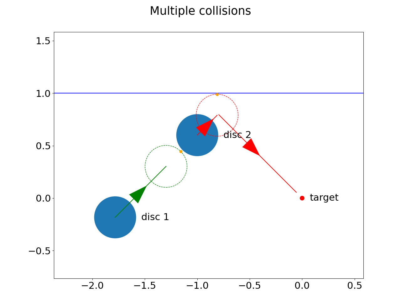
(a) Initial configurations

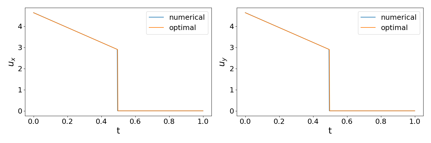
(b) Shape of the optimal control

Fig. 7: Illustration of the multiple collisions in Section 5.3. LABEL:sub@fig:case4_illustration Initial state: The initial locations of discs are the blue discs. The green and red lines are optimal trajectories of disc 1 and disc 2, respectively. The dashed green circle is the position of disc 1 when disc 1 collides with disc 2. The dashed red circle is the position of disc 2 when disc 2 collides with the wall. The orange points are the collision points. The blue line represents the wall. LABEL:sub@fig:case4_shape The numerical optimal control and the analytical optimal control, $\bm{u}=[\bm{u}_{x},\bm{u}_{y}]$.

We discretize the dynamics into 480 steps, i.e. $N=480$ and run the Algorithm 2 with the relaxation parameter $\alpha=0.01$. The initial control is the constant control pointing disc 2 from disc 1 with magnitude $3\sqrt{2}$, i.e. $[3,3]^{T}$. The numerical result is shown and compared to the analytical one in Figure 7b. Again, linear convergence is observed, and a few hundred iterations are enough for the algorithm to converge, see Figure 8.

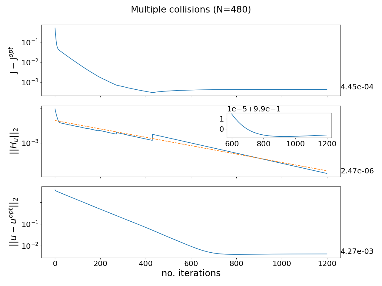
Fig. 8: The example of multiple collisions in Section 5.3: the convergence of the iterative algorithm. The annotations on the right are the final values of the corresponding curves. The common $x$ axis is the number of iterations spent in the Algorithm 2. Top: the difference between the analytical optimal objective and the numerical solutions. Middle: the $L^{2}$ semi-norm of the derivative of the Hamiltonian with respect to the control $\bm{u}$. The dashed line is the result of the regression in the form $\mu\sigma^{k}$ (this is the linear regression after taking the logarithm. $k$ is the number of iterations, $\mu,\sigma$ are positive regression parameters). The inset plot is the ratio $\|H_{u}^{k+1}\|_{2}/\|H_{u}^{k}\|_{2}$ versus the number of iterations. Bottom: the difference between the analytical optimal control and the numerical solutions in terms of the $L^{2}$ semi-norm.

As depicted in Figure 9, our optimal numerical control is approaching the analytical solution as $\Delta t$ approaches zero and the collision times also converge to the analytical ones. We also note that the order of accuracy is still first order. It does not degrade with more collisions.

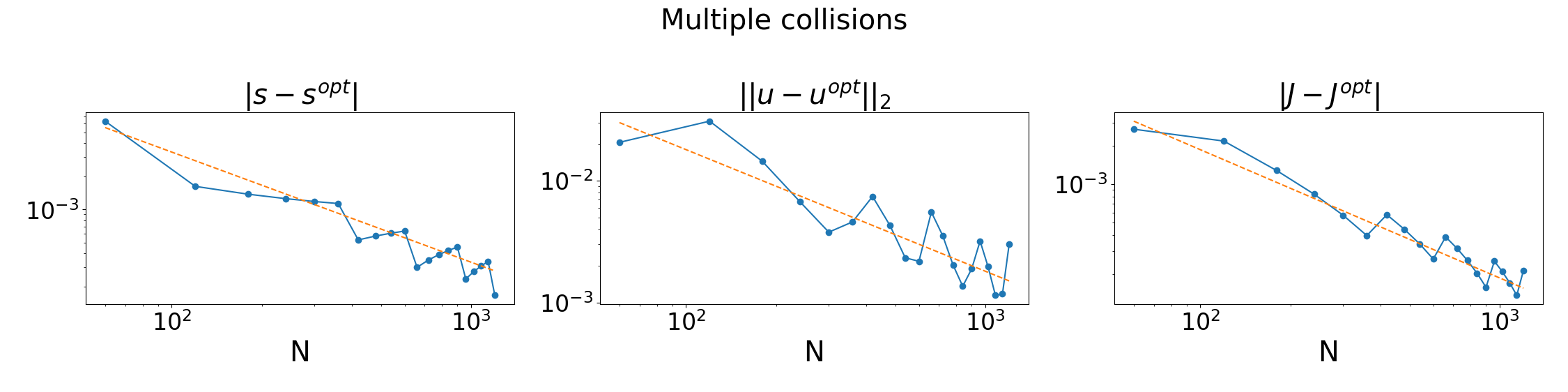
Fig. 9: The example of multiple collisions in Section 5.3: convergence to the analytical solution when the number of time intervals $N$ tends to infinity. The dashed orange lines are straight lines obtained by the least square regression on the data with model $\sigma/N$ and parameter $\sigma$. Left: Difference between the simulated collision times and the analytical optimal collision time. Middle: Difference between the numerical and analytical solutions for the optimal controls in terms of $L^{2}$ semi-norm. Right: Difference between the simulated total costs and the optimal analytical solution.

5.4 $L^{1}$ running cost

To further demonstrate the performance of the proposed algorithm, we reconsider the example in Section 5.2, a general collision of two discs, but with a different (non-quadratic) running cost,

$$L(\bm{x},\bm{u})=\epsilon|\bm{u}|,$$

under the constraint $|\bm{u}|\leq u_{M}$. Namely, we have

$$U=\{(\bm{u}_{x},\bm{u}_{y})\in\mathbb{R}^{2}:\bm{u}_{x}^{2}+\bm{u}_{y}^{2}\leq u_{M}^{2}\}.$$

The associated Hamiltonian is

$$H(\bm{x},\bm{\lambda},\bm{u})=\bm{\lambda}_{q_{1}}\cdot\bm{x}_{v_{1}}+\bm{\lambda}_{q_{2}}\cdot\bm{x}_{v_{2}}+\frac{1}{m_{1}}\bm{\lambda}_{v_{1}}\cdot\bm{u}+\epsilon|\bm{u}|.$$ (50)

Its minimizer with respect to $\bm{u}$ is

$$\bm{u}_{*}=\arg\min_{\bm{u}\in U}H(\bm{x},\bm{\lambda},\bm{u})=-u_{M}\frac{\bm{\lambda}_{v_{1}}}{|\bm{\lambda}_{v_{1}}|}$$ (51)

when $|\bm{\lambda}_{v_{1}}|\geq m_{1}\epsilon$ and $0$ otherwise. We take $u_{M}=5\sqrt{2}$ and $\epsilon=0.01$ in the experiment. The optimal control, numerically solved, is visualized in Figure 10a. We also plot the direction of $\bm{\lambda}_{v_{1}}$ and $\bm{u}\cdot\bm{\lambda}_{v_{1}}/|\bm{\lambda}_{v_{1}}|$. At the final iteration, $|\bm{\lambda}_{v_{1}}|>m_{1}\epsilon$ before the collision and $|\bm{\lambda}_{v_{1}}|=0$ after the collision. The projection $\bm{u}\cdot\bm{\lambda}_{v_{1}}/|\bm{\lambda}_{v_{1}}|$ achieves its minimum value $-u_{M}$ before the collision, which shows that the obtained control minimizes the Hamiltonian (50) according to eq. 51. Finally, as depicted in Figure 10b, the total objective decreases with iterations and converges. We have also tested a different constraint set $U$ that imposes constraints on control componentwisely in this example and the example of concentric collision in Section 5.1. In all these examples with $L^{1}$ running cost, the proposed algorithm converges without any further tuning.

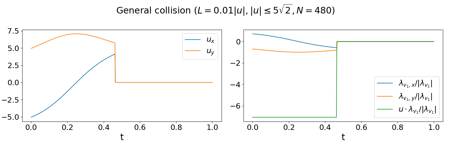
(a) The optimal control

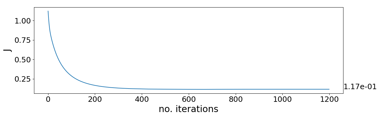
(b) Total costs

Fig. 10: Illustration of the general collision with $L^{1}$ running cost in Section 5.4. LABEL:sub@fig:gc_l1_norm_shape Left: The numerical optimal control $\bm{u}=[\bm{u}_{x},\bm{u}_{y}]$. Right: The direction of $\bm{\lambda}_{v_{1}}=[\bm{\lambda}_{v_{1},x},\bm{\lambda}_{v_{1},y}]$ and the projection of $\bm{u}$ to it. LABEL:sub@fig:gc_l1_norm_cost The objective versus iterations.

5.5 Comparison to HMP-MAS

In [46], given the number of switching times, the author proposed to solve the optimal control in multiple autonomous switchings system based on the hybrid maximum principle (HMP-MAS) by alternating between (1) solving for optimal controls in the sub-domains divided by guessed switching time and switching states; (2) computing gradients and updating the guesses by gradient descent. The method has been extended to autonomous hybrid dynamical systems on manifolds [53, 54]. Recently, it has been extended to the autonomous hybrid dynamical systems with both state jumps and switches in dynamics in [38]. We adapt this method to the dynamical systems discussed in this paper.

To be specific, we assume that there will be one collision for the optimal control. Starting from a reasonable guess that the collision happens at $t=s$ and at state $\bm{x}_{s}^{-}$, we solve two standard optimal control problems: find the minimal cost control that shoots $(s,\bm{x}_{s}^{-})$ from $(0,\bm{x}_{0})$ and find the optimal control that minimizing the running cost and terminal cost starting from $\bm{x}_{s}^{+}$ at $t=s$. Then, one can compute the gradient of the total cost with respect to $s$ and $\bm{x}_{s}^{-}$ and then update them by gradient descent. The constraint $\phi(\bm{x}_{s}^{-})=0$ is enforced as a penalty added to the total costs.

The overall performance of this algorithm is comparable to our algorithm, exhibiting a similar convergence curve and error. However, one needs to prescribe the correct number of collisions beforehand for this method. We run the multiple collisions experiment (section 5.3) starting from an initial trajectory with three collisions (see Figure 11). Our algorithm converges to the optimal control with two collisions without any modifications. In contrast, HMP-MAS cannot converge to the optimal solution starting from such an initialization.

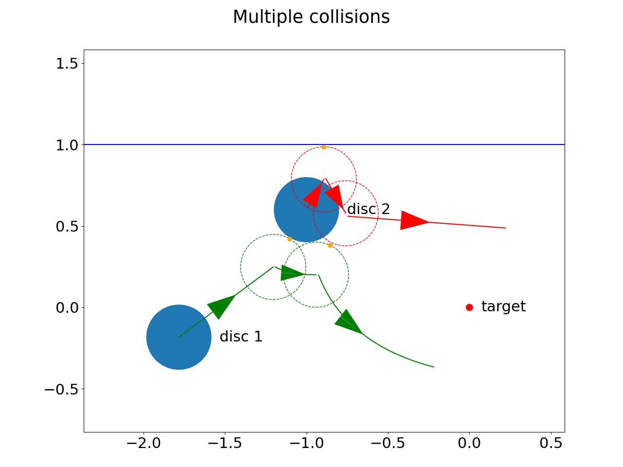
Fig. 11: Illustration of the trajectories under a control that results in three collisions. The green and red lines with arrows are trajectories of disc 1 and disc 2, respectively. Dashed green circles and red circles are snapshots of disc 1 and disc 2 when collisions occur, respectively. The orange points are collision points. See Section 5.5.

5.6 Comparison to a direct method

In this subsection, we compare Algorithm 2 with a gradient descent algorithm, which is applied to the following discretized problem

$$\mathmakebox[\widthof{$\underset{\displaystyle u_{0},\cdots,u_{N-1}}{\mathrm{subject~{}to}}$}][l]{\underset{\displaystyle u_{0},\cdots,u_{N-1}}{\mathrm{minimize}}}\quad\phi(\bm{x}_{N})+\sum_{i=0}^{N-1}L(\bm{x}_{i},\bm{u}_{i})\Delta t,$$ (52a)

$$\mathmakebox[\widthof{$\underset{\displaystyle\phantom{u_{0},\cdots,u_{N-1}}}{\mathrm{subject~{}to}}$}][c]{{\mathrm{subject~{}to}}}\quad \lx@cref{creftype~refnum}{eq:fd_all_in_one_dis}.$$ (52b)

The discrete dynamics is implemented in PyTorch [41] with gradients with respect to the controls $\bm{u}_{0},\cdots,\bm{u}_{N-1}$ been calculated by auto-differentiation.

The learning rate is chosen to be compatible with Algorithm 2. For the examples considered in this paper, the continuous version of the control update step in Algorithm 2, i.e. eq. 22, can be rewritten as

$$\bm{u}^{k+1}=(1-\alpha)\bm{u}^{k}+\alpha\bm{u}_{*}=\bm{u}^{k}-\frac{\alpha}{2\epsilon}H_{u}(\bm{x}^{k},\bm{\lambda}^{k},\bm{u}^{k}),$$

recalling the minimizer $\bm{u}_{*}$ in eq. 45 and $H_{u}$ in eq. 46. Therefore, we set the learning rate to $\frac{\alpha N}{2\epsilon}$, where the factor $N$ is multiplied to compensate the integration step size $\Delta t$ since the discrete gradient has an additional time step factor $\Delta t$ compared to its continuous counterpart. We note that selecting a consistent learning rate is only for the purpose of comparison. As can be seen in Figure 12, the learning curves of these two methods overlap at the beginning of the iteration. Further changes to the learning rate and more training iterations will not lead to a reduction in the error of the solution for the direct method.

We have compared the performance of Algorithm 2 and the direct method at $N=480$ on all three examples considered previously, and the comparison is shown in Figure  12. We find that our HMP-based algorithm always performs much better than the direct method; the numerical solution of the optimal control and the corresponding total cost of the Algorithm 2 are much closer to their analytical ones.

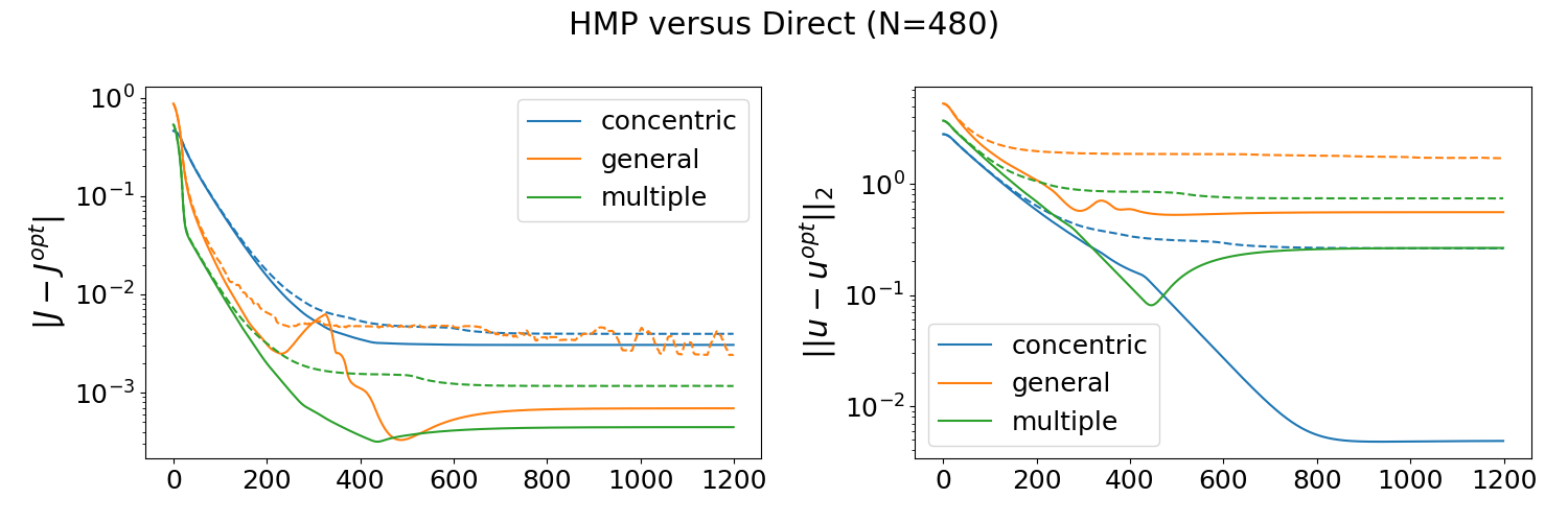
Fig. 12: The comparison between HMP (Algorithm 2) and the direct method over all three experiments; the concentric collision (section 5.1), the general situation (section 5.2) and the multiple collisions (section 5.3). Solid line are data from the Algorithm 2. Dashed lines are data from the direct method; Different colors correspond to different experiments, see legends in the figure. Left: Difference between the simulated total costs and the optimal analytical total costs. Right: Difference between the numerical controls and analytical optimal controls in terms of $L^{2}$ semi-norm. See Section 5.6.

The convergence behavior as $N\rightarrow\infty$ is also compared, see Figures in 13. As seen from the figure, the direct method also produces reasonable solutions in terms of the total costs but does not converge well; the errors to the optimal analytical controls measured in $L^{2}$ semi-norm show no signs of convergence as $N$ increases. Similar behavior has been observed in the collision times. The direct method produces comparable results regarding the total costs in the concentric collision example and multiple collisions example but still fails to converge in the general situation example.

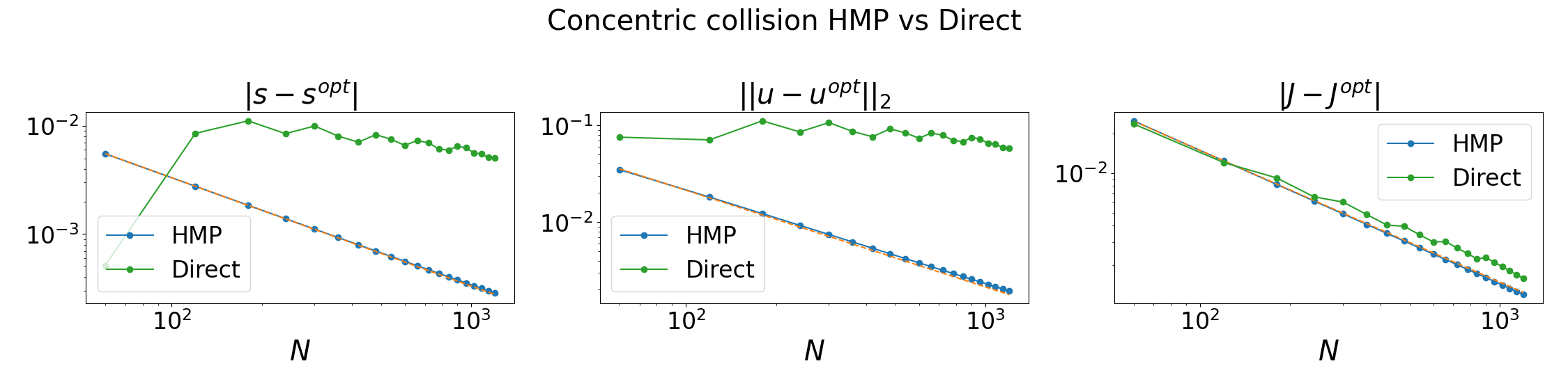
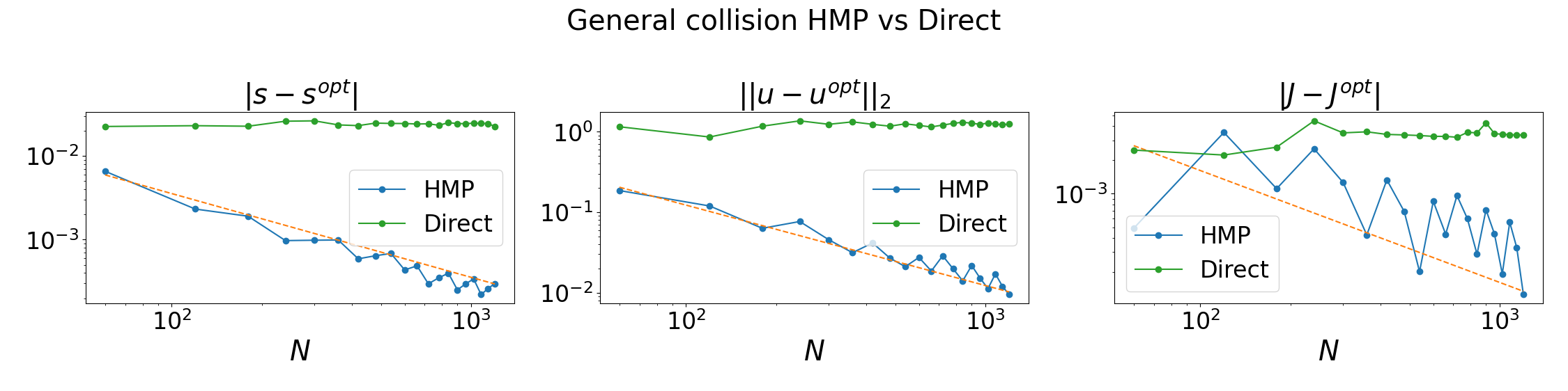
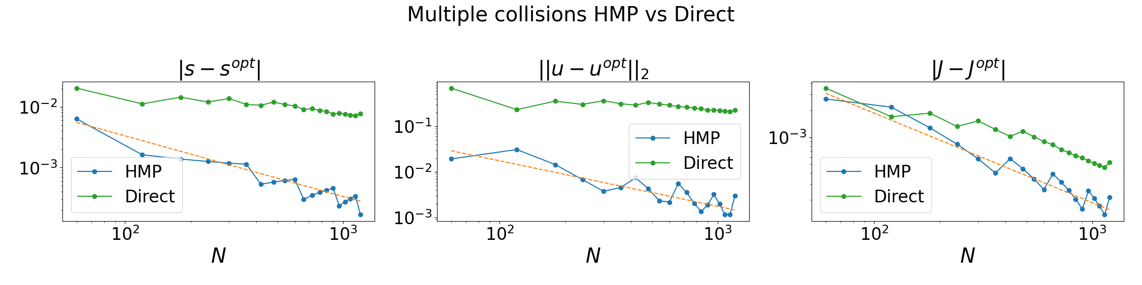
Fig. 13: Convergence to the analytical solution as $N$ increases. The dashed orange lines are straight lines obtained by the least square regression on the results of Algorithm 2 with model $\sigma/N$ and parameter $\sigma$. Top: The concentric collision example (section 5.1). Middle: The general situation example (section 5.2). Bottom: The multiple collisions example (section 5.3). Left: Difference between the simulated collision times and the analytical optimal collision times. Middle: Difference between the numerical controls and the analytical optimal controls in terms of $L^{2}$ semi-norm. Right: Difference between the simulated total costs and the optimal analytical solutions. See Section 5.6

.

Despite the fact that their gradients are related, the HMP algorithm and the gradient descent algorithm are still quite different. Numerically, the difference can be seen in Figures 12 and 13. Conceptually, for general forms of the dynamics and cost functional, the update direction in the HMP algorithm based on the stronger minimization conditions (eq. 12) is not parallel to the gradient direction. As pointed out in [51, 24], the gradient of the discrete problem might be incorrect (in the sense that it does not converge to that of the continuous problem). In some cases (like the examples considered in this paper) where the minimization direction coincides with the gradient direction, due to the discontinuities, the numerical approximation of the Fréchet derivatives $H_{u}$ (of the HMP algorithm, see Remark 3 and eq. 34) are different from the gradients of the discrete problems (of the direct method, see eq. 52). Another point worth noting is that in the HMP algorithm, we can stabilize the numerical computations of $H_{u}$ (e.g. eqs. 28 and 29 in the discretization of the backward dynamics) from the continuous point of view. As discussed in Section 4, this is of critical importance for the dynamics with discontinuities. In contrast, it is unclear how to adopt similar stabilization techniques for the direct method.

5.7 Comparison to deep reinforcement learning

Deep reinforcement learning has demonstrated its ability in many complex tasks [33, 32, 49, 50, 34]. In this section, we reformulate the optimal control problem considered in this paper into a reinforcement learning problem and test the performance of a modern advanced deep reinforcement learning algorithm: the Proximal Policy Optimization (PPO) algorithm [45].

We take the example of the concentric collision in section 5.1. The observation space is the time-state space $\mathbb{R}^{9}=(t,\bm{x}),t\in[0,T],\bm{x}\in\mathbb{R}^{8}$. The action space is the two-dimensional control whose components are scaled to $[-1,1]$,

$$\bar{\bm{u}}=\frac{\bm{u}+5}{10}.$$

Here, we assume that each component of the actual control takes values in $[-5,5]$. We use Stable-Baselines 3 [44] to implement the PPO algorithm. We use two-layer neural networks for the actor and critic networks; each layer has 64 neurons. Each episode in the training consists of $N=60$ time steps.

As discussed previously, due to the control cost, the randomly initialized policy network will quickly converge to zero. It is necessary to encourage exploration by using a warm-up step. This is done by setting the running cost $L$ to zero in the early training stage. We train the warm-up stage for $3000$ episodes. The policy network starts converging after a series of actions that triggers a collision is exploited. See the inset of the right subfigure of Figure 14. Afterwards, we restore the running cost defined in eq. 43 and train for another $80000$ episodes.

The convergence history of the rewards and the profile of the best control policy are shown in Figure 14. We observe that the best policy is obtained at around $3000+60000$ episodes. After that, the control network starts converging to zero. The best policy found is still far from optimal. The optimal total cost found by the PPO algorithm is $1.617140$, which is $15.80\%$ suboptimal to the optimal cost of $1.396542$. Note that the optimal cost found by Algorithm 2 is $1.421552$.

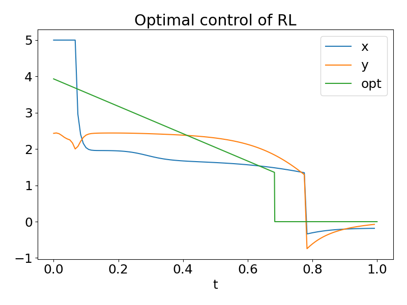
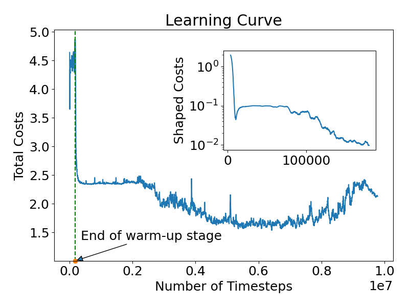
Fig. 14: The performance of the deep reinforcement learning algorithm (PPO) described in section 5.7 on the example of concentric collision. Left: the optimal control found by the PPO. Curves labelled with $x,y$ are the $x,y$ components of the control, respectively. The green curve labeled with “opt” is the analytical optimal control (its $x,y$ components are the same). Right: the evolution of the total cost versus training steps. The modified costs (with running costs dropped) are plotted for the warm-up stage in the inset plot at log scale.

6 Summary and future work

This paper presents a numerical algorithm for finding the optimal control of dynamical systems with autonomous state jumps. We consider the dynamical system that models the collisional rigid body dynamics, a critical component of many practical applications. We address the challenges posed by the presence of discontinuities both theoretically and numerically. On the theoretical side, we present the strong collision condition, analyze the stability of collision, and prove a theorem on linear convergence. In addition, we suggest various numerical techniques to mitigate the effects of discontinuities. We test the proposed algorithm on several examples in which the optimal controls drive the discs to collide in order to achieve the lowest total cost. Comparisons to HMP-MAS, the direct method, and deep reinforcement learning demonstrate the superiority of the proposed algorithm in terms of accuracy, efficiency, and flexibility. Implemented with the forward-Euler scheme, the algorithm shows linear convergence with respect to the iteration steps and asymptotic first-order accuracy in terms of time discretization.

The proposed method can be extended in a few directions.

General shapes

In general, there are more complex-shaped rigid bodies. These shapes introduce additional challenges in computing both the functions and their derivatives of the collision detection functions $\psi$ and the jump functions $g$. Besides, angular quantities such as orientation, angular velocity, and torques are often needed to describe the system. These quantities can still be fully characterized under the formulation in Section 2.

Contact dynamics and plastic collisions

Contacts are another essential feature in many applications. They can be viewed as continuous collisions in certain time intervals. Examples range from robotic arms, e.g. fetch environments (the FetchPush and FetchSlide [42]) to quadrupeds [25] and humanoids [56, 29]. Instead of modeling their dynamics by continuous collisions, we may formulate them as autonomous switching dynamical systems. When entering the contact surface and under an applied impulse, the right-hand side function $f$ changes discontinuously. The plastic collision, after which the objects coalesce, has a similar behavior; i.e. the inertia components in $f$ switch from the individual ones to a composite one [37]. As mentioned earlier, the dynamical systems can be formulated as in Section 2 and a corresponding HMP can be derived. A successive approximation type algorithm can be constructed similar to that in Section 4.

Frictional dynamics

Frictional force is critical in many applications, from simple models like the hopper [19] and swimmer [16], to complex models like quadrupeds [25] and humanoids [56, 29]. The frictional forces are always present together with contacts/collisions. Frictions introduce extra discontinuity and nonlinearity to the dynamical system, in addition to collisions and contacts. They can be viewed as a set-valued function consisting of two modes; the following formula is a one-dimensional example,

$$f(v)\in\begin{cases}\{-\mu N\}\quad&\text{if }v>0\\ \{\mu N\}\quad&\text{if }v<0\\ [-\mu N,\mu N]\quad&\text{if }v=0\end{cases},$$

where $\mu$ is the frictional coefficient, $N$ is the normal contact force, and $v$ is the relative velocity.

Frictional dynamics can also be described in the framework of switching systems. The presence of frictions adds additional dependency of the discontinuities on the state, i.e. the relative velocity. In addition, it is usually a source of nonlinearity since friction takes value in a cone determined by the magnitude of the normal contact force, which is a more complex function of the state.

Convergence guarantee and algorithm improvement

In this paper, we have proven that the vanilla MSA algorithm converges linearly for the optimal control problem with collisions under certain requirements. Additionally, we have demonstrated that the proposed relaxed MSA algorithm performs well in several typical examples. We analyze the stability of collision, which is crucial for discontinuous optimal control problems. However, we have not yet studied how much relaxation can help loosen convergence requirements. Furthermore, there exist more sophisticated techniques to improve the algorithm, such as doing a line search instead of fixing $\alpha$, or using adaptive update schemes as presented in [15, 30]. These methods may be helpful for more challenging problems that involve highly nonlinear dynamics and more complex discontinuous behaviors. A thorough study of applying various techniques to discontinuous optimal control problems and the corresponding convergence analysis is left for future research.

Appendix A Analytical optimal controls

The common parameters are summarized in Table 1. In the examples considered, the optimal control should drive disc 1 to collide with disc 2 so that disc 2 is close to the origin at the terminal time $T=1$. Recall that we always assign zero initial velocity to disc 2. Let us assume that disc 1 collides with disc 2 with velocity $\bm{v}^{\prime}$ at the collision time $s$. The after collision velocity of disc 2 is $\bm{v}=(\bm{v}^{\prime}\cdot\mathbf{n})\mathbf{n}$, see Section 5. The displacement of disc 1 before collision is a linear function of $\mathbf{n}$,

$$\bm{d} =\bm{q}_{1}(s)-\bm{q}_{1}(0)=\bm{q}_{2}(s)-(r_{1}+r_{2})\mathbf{n}-\bm{q}_{1}(0)$$

$$=\bm{q}_{2}(0)-\bm{q}_{1}(0)-(r_{1}+r_{2})\mathbf{n}.$$ (53)

Here, $\bm{q}_{1},\bm{q}_{2}$ are the positions of disc 1, disc 2, respectively. Given the collision time $s$, the collision velocity $\bm{v}^{\prime}$ and the contact normal $\mathbf{n}$, the optimal control $\bm{u}$ before collision can be obtained by solving,

$$\mathmakebox[\widthof{$\underset{\displaystyle u}{\mathrm{subject~{}to}}$}][l]{\underset{\displaystyle u}{\mathrm{minimize}}}\quad\int_{0}^{s}L(\bm{x},\bm{u})dt$$ (54a)

$$\mathmakebox[\widthof{$\underset{\displaystyle\phantom{u}}{\mathrm{subject~{}to}}$}][c]{{\mathrm{subject~{}to}}}\quad \int_{0}^{s}\bm{u}(t)~{}dt=\bm{v}^{\prime},$$ (54b)

$$\int_{0}^{s}(s-t)\bm{u}(t)~{}dt=\bm{d}.$$ (54c)

The optimal control after collision is identically zero. In the case $L(\bm{x},\bm{u})=\epsilon|\bm{u}|^{2}$, the optimal control before collision is

$$\bm{u}(t)=\frac{6\bm{d}}{s^{2}}-\frac{2\bm{v}^{\prime}}{s}+(\frac{6\bm{v}^{\prime}}{s^{2}}-\frac{12\bm{d}}{s^{3}})t.$$ (55)

Then, the total cost is

$$\phi(\bm{x}(T))+\int_{0}^{T}L(\bm{x},\bm{u})~{}dt$$

$$=~{} |\bm{q}_{2}(s)+(T-s)(\bm{v}^{\prime}\cdot\mathbf{n})\mathbf{n}|^{2}+\epsilon(\frac{12}{s^{3}}|\bm{d}|^{2}+\frac{4}{s}|\bm{v}^{\prime}|^{2}-\frac{12}{s^{2}}\bm{v}^{\prime}\cdot\bm{d}).$$ (56)

Recall that $\bm{d}$ is a linear function of $\mathbf{n}$ and $\bm{q}_{2}(s)=\bm{q}_{2}(0)$. The objective 56 depends only on $s,\bm{v}^{\prime}$ and $\mathbf{n}$.

Example 5.1

In the configuration described in Section 5.1 where the concentric collision is preferred, the optimal $\mathbf{n}=\frac{1}{\sqrt{2}}(1,1)$, and the optimal $\bm{v}$ takes the form $\bm{v}=(v_{c},v_{c}),v_{c}\in\mathbb{R}$. Then the total cost 56 is quadratic in $v_{c}$, whose optimal value can be analytically solved as a function of $s$. Finally, we turn the total cost into a rational function of $s$, whose minimizer in $(0,T)$ can be computed using an analytical solution to machine accuracy.

Example 5.2

In the the general situation described in Section 5.2, one cannot solve the optimal contact normal vector easily. Note that the total cost (56) is quadratic in $\bm{v}^{\prime}$, we can first minimize it with respect to $\bm{v}^{\prime}$. To this end, we set the gradient of the total cost with respect to $\bm{v}^{\prime}$ to zero to have

$$\bm{v}^{\prime}\cdot\mathbf{n}^{\perp}=\frac{3\bm{d}\cdot\mathbf{n}^{\perp}}{2s},\bm{v}^{\prime}\cdot\mathbf{n}=-\frac{s^{2}(T-s)\bm{q}_{2}(0)\cdot\mathbf{n}-6\epsilon\bm{d}\cdot\mathbf{n}}{4\epsilon s+s^{2}(T-s)^{2}},$$ (57)

where $\mathbf{n}^{\perp}=\big{(}\begin{smallmatrix}0&-1\\ 1&0\end{smallmatrix}\big{)}\mathbf{n}$ is obtained by rotating $\mathbf{n}$ 90 degrees. Then, the total cost (56) is rational in $s$ and is a fourth-order polynomial in the coordinates of $\mathbf{n}$. The constraints are $|\mathbf{n}|^{2}=1$ and $s\in(0,T)$. Therefore, minimization of the total cost can be solved to machine accuracy using an analytical solution.

Example 5.3

In the multiple collisions example described in Section 5.3, the velocity of a disc with velocity $\bm{v}=(\bm{v}_{x},\bm{v}_{y})$ becomes $(\bm{v}_{x},-\bm{v}_{y})$ after a collision with the wall $y=b$. Let us denote the velocity of disc 2 after the collision with disc 1 by $\bm{v}=(\bm{v}_{x},\bm{v}_{y})$. It takes time $(b-r_{2}-\bm{q}_{2,y}(s))/\bm{v}_{y}$ for disc 2 to collide with the wall, where $\bm{q}_{2,y}(s)$ is the $y$ coordinate of the position of disc 2 at time $s$. Thus, the terminal cost is

$$|\bm{q}_{2,x}(s)+\bm{v}_{x}(T-s)|^{2}+|(b-r_{2})-\bm{v}_{y}(T-s-\frac{b-r_{2}-\bm{q}_{2,y}(s)}{\bm{v}_{y}})|^{2}$$

$$=~{} |\bm{q}_{2,x}(s)+\bm{v}_{x}(T-s)|^{2}+|\bm{q}_{2,y}(s)+(T-s)\bm{v}_{y}-2(b-r_{2})|^{2},$$

namely, the square distance to the point $(0,2(b-r_{2}))$ as if there is no wall. The optimal control for this case can be computed using the same procedure as in the previous examples.

Appendix B Proof of convergence

The main goal of this section is to prove Theorem 4 and Theorem 5. Throughout this section, we always assume that Assumptions 1, 2, 3, 4, 5 and 6 hold. With these assumptions, it is obvious that the state, costate, and control are piecewise smooth during the iteration. Additionally, Theorems 4 and 5 suggest that we should mainly focus on functions that are piecewise smooth with two pieces.

Definition 7 (Piecewise smooth with two pieces functions).

We say a function $\bm{v}\colon[0,T]\rightarrow\mathbb{R}^{k}$ is piecewise smooth with two pieces if there is a point $\beta\in(0,T)$ such that $\bm{v}$ is smooth in closed intervals $[0,\beta]$ and $[\beta,T]$, up to possible redefinition at $\beta$ when restricting to each interval.

We denote the one-sided limits of a piecewise smooth with two pieces function, which is discontinuous at $\beta$, as

$$\bm{v}^{-}=\lim_{t\rightarrow\beta^{-}}\bm{v}(t),\;\bm{v}^{+}=\lim_{t\rightarrow\beta^{+}}\bm{v}(t).$$ (58)

We will always use the symbol $\beta$ to denote the discontinuities of the control and $\gamma$ to denote the discontinuities of the state. For simplicity, we denote

$$\|\dot{\bm{v}}\|_{\infty}=\max\{\|\dot{\bm{v}}\|_{L^{\infty}(0,\beta)},\|\dot{\bm{v}}\|_{L^{\infty}(\beta,T)}\}$$

for any piecewise smooth with two pieces function $\bm{v}$ that is discontinuous at $\beta$. For piecewise smooth with two pieces functions $\bm{u}_{1},\bm{u}_{2}$ with discontinuities at $\beta_{1},\beta_{2}$, we recall the semimetric $\mathfrak{d}(\cdot,\cdot)$:

$$\mathfrak{d}(\bm{v}_{1},\bm{v}_{2})=\max\{\|\bm{v}_{1}-\bm{v}_{2}\|_{L^{\infty}(0,\min\{\beta_{1},\beta_{2}\})},\|\bm{v}_{1}-\bm{v}_{2}\|_{L^{\infty}(\max\{\beta_{1},\beta_{2}\},T)},|\beta_{1}-\beta_{2}|\}.$$

We note that it is a semimetric satisfying $\mathfrak{d}(\bm{u}_{1},\bm{u}_{2})=0$ if and only if $\bm{u}_{1}=\bm{u}_{2}$, and $\mathfrak{d}(\bm{v}_{1},\bm{v}_{2})=\mathfrak{d}(\bm{v}_{2},\bm{v}_{1})$. We note that two piecewise smooth with two pieces functions are equal to each other if they break at the same point and they are equal pointwise, except at the breakpoint.

In developing theorems, we will encounter many constants. For simplicity, we introduce the following definition.

Definition 8.

We say a positive constant depends only on the optimal control problem if it only depends on the bounds $M_{u}$ and the functions defining the optimal control problem, i.e. $\bm{f},\bm{g},\psi,\phi,L$, through their smoothness constants in Assumption 3, their values at a fixed point in their domain, and the total time $T$.

Before delving into more details, we first prove two lemmas relating to the used semimetric. The first lemma is an estimate of side limits of the piecewise smooth with two pieces controls:

Lemma 9.

If $\bm{u}_{1},\bm{u}_{2}\in L^{1}(0,T;\mathbb{R}^{m})$ are piecewise smooth with two pieces function. Then,

$$|\bm{u}_{1}^{+}-\bm{u}_{2}^{+}|+|\bm{u}_{1}^{-}-\bm{u}_{2}^{-}|$$

$$\leq (2+\|\dot{\bm{u}}_{1}\|_{\infty}+\|\dot{\bm{u}}_{2}\|_{\infty})\mathfrak{d}(\bm{u}_{1},\bm{u}_{2})$$

where $\beta_{1},\beta_{2}\in(0,T)$ are breakpoints of $\bm{u}_{1},\bm{u}_{2}$ and $\bm{u}_{1}^{\pm},\bm{u}_{2}^{\pm}$ are one-sided limits at corresponding breakpoints, respectively.

Proof.

Without loss of generality, we assume $\beta_{1}\leq\beta_{2}$.

$$|\bm{u}_{1}^{-}-\bm{u}_{2}^{-}|\leq |\bm{u}_{1}^{-}-\bm{u}_{2}(\beta_{1})|+|\bm{u}_{2}(\beta_{1})-\bm{u}_{2}^{-}|$$

$$= |\lim_{t\rightarrow\beta_{1}^{-}}\bm{u}_{1}(t)-\bm{u}_{2}(\beta_{1})|+|\bm{u}_{2}(\beta_{1})-\lim_{t\rightarrow\beta_{2}^{-}}\bm{u}_{2}(t)|$$

$$\leq \|\bm{u}_{1}-\bm{u}_{2}\|_{L^{\infty}(a,\beta_{1})}+\|\dot{\bm{u}}_{2}\|_{L^{\infty}(\beta_{1},\beta_{2})}|\beta_{1}-\beta_{2}|$$

$$\leq \mathfrak{d}(\bm{u}_{1},\bm{u}_{2})+\|\dot{\bm{u}}_{2}\|_{L^{\infty}(\beta_{1},\beta_{2})}|\beta_{1}-\beta_{2}|.$$

Similarly,

$$|\bm{u}_{1}^{+}-\bm{u}_{2}^{+}|\leq\mathfrak{d}(\bm{u}_{1},\bm{u}_{2})+\|\dot{\bm{u}}_{1}\|_{L^{\infty}(\beta_{1},\beta_{2})}|\beta_{1}-\beta_{2}|.$$

Therefore,

$$|\bm{u}_{1}^{+}-\bm{u}_{2}^{+}|+|\bm{u}_{1}^{-}-\bm{u}_{2}^{-}|$$

$$\leq 2\mathfrak{d}(\bm{u}_{1},\bm{u}_{2})+(\|\dot{\bm{u}}_{1}\|_{\infty}+\|\dot{\bm{u}}_{2}\|_{\infty})|\beta_{1}-\beta_{2}|$$

$$\leq (2+\|\dot{\bm{u}}_{1}\|_{\infty}+\|\dot{\bm{u}}_{2}\|_{\infty})\mathfrak{d}(\bm{u}_{1},\bm{u}_{2}).$$

∎

The second lemma shows that the semimetric is stronger than $L^{1}$.

Lemma 10 (Control $L^{1}$ by semimetric).

For any control $\bm{u}_{1},\bm{u}_{2}\in(L^{1}\cap L^{\infty})(0,T;U)$, we have,

$$\|\bm{u}_{1}-\bm{u}_{2}\|_{1}\leq C_{1,\infty}\mathfrak{d}(\bm{u}_{1},\bm{u}_{2}),$$ (59)

where $C_{1,\infty}$ only depends on the optimal problem.

Proof.

Without loss of generality, assume $\beta_{1}<\beta_{2}$,

$$\int_{0}^{T}|\bm{u}_{1}-\bm{u}_{2}|~{}dt$$

$$= \int_{0}^{\beta_{1}}|\bm{u}_{1}-\bm{u}_{2}|~{}dt+\int_{\beta_{1}}^{\beta_{2}}|\bm{u}_{1}-\bm{u}_{2}|~{}dt+\int_{\beta_{2}}^{T}|\bm{u}_{1}-\bm{u}_{2}|~{}dt$$

$$\leq \beta_{1}\|\bm{u}_{1}-\bm{u}_{2}\|_{L^{\infty}(0,\beta_{1})}+2M_{u}|\beta_{1}-\beta_{2}|+(T-\beta_{2})\|\bm{u}_{1}-\bm{u}_{2}\|_{L^{\infty}(\beta_{2},T)}$$

$$\leq (T+2M_{u})\mathfrak{d}(\bm{u}_{1},\bm{u}_{2}).$$

∎

Outline of proof

We present boundedness and estimates of the state in sections B.2 and B.3. This part of our work is similar to classical theories of ordinary differential equations. Additionally, we establish the stability of collision (Theorem 4) in section B.4. This stability primarily depends on state estimates and a local expansion of the collision detection function $\psi(\bm{x}(t))$. We incorporate the strong collision condition to analyze the sign of $\psi(\bm{x}(t))$ near the collision time, allowing us to control its root by Rolle’s theorem. Furthermore, we demonstrate boundedness and estimates of costate in sections B.5 and B.6. The discontinuity of our model presents some difficulties, as the term $\psi_{x}\bm{f}$ appears in the denominator of the costate jump function. The strong collision condition provides a positive margin to ensure that the denominator stays away from zero. We provide estimations there and defer a uniform positive margin to section B.7. Finally, we use our estimates for state and costate, as well as our stability analysis of the collision, to prove Theorem 5 in section B.7.

B.1 The strong collision condition

We recall the strong collision condition with positive $a,b,K,S$ for $\bm{u}$ implies

$$v(\gamma^{-})=\psi_{x}(\bm{x}(\gamma^{-}))\cdot\bm{f}(\bm{x}(\gamma^{-}),\bm{u}(\gamma^{-}))\leq-K\leq-(S+B_{f,u}M_{J}(\bm{u})),$$

where we denote,

$$v(t)\coloneqq\psi_{x}(\bm{x}(t))\cdot\bm{f}(\bm{x}(t),\bm{u}(t))=\frac{d}{dt}\psi(\bm{x}(t)).$$ (60)

Assumption 3 (Smoothness) gives us the ability to estimate $v(t)$ as shown in Lemma 11.

Lemma 11.

If $\bm{u}$ is smooth for $t<\gamma$, then we have,

$$|v(t)-v(\gamma^{-})|\leq C|t-\gamma|,$$

the constant $C$ depends only on the optimal control problem and $\|\dot{\bm{u}}\|_{\infty}$.

Proof.

Using the Lipschitz continuity, we have,

$$|v(t)-v(\gamma^{-})|$$

$$\leq |[\psi_{x}(\bm{x}(t))-\psi_{x}(\bm{x}(\gamma^{-}))]\cdot\bm{f}(\bm{x}(t),\bm{u}(t))|$$

$$+|\psi_{x}(\bm{x}(\gamma^{-}))\cdot[\bm{f}(\bm{x}(t),\bm{u}(t))-\bm{f}(\bm{x}(\gamma^{-}),\bm{u}(\gamma^{-}))]|$$

$$\leq M_{f}B_{\psi_{x}}|\bm{x}(t)-\bm{x}^{-}|+B_{f,x}|\bm{x}(t)-\bm{x}^{-}|+B_{f,u}|\bm{u}(t)-\bm{u}^{-}|$$

$$\leq (M_{f}B_{\psi_{x}}+B_{f,x})M_{f}|t-\gamma|+B_{f,u}\|\dot{\bm{u}}\|_{\infty}|t-\gamma|,$$

where we applied $|\bm{x}(t)-\bm{x}^{-}|\leq\int_{t}^{\gamma}|\dot{\bm{x}}(s)|~{}ds\leq M_{f}|t-\gamma|$ and $|\psi_{x}(\bm{x}(\gamma^{-}))|=1$. Let

$$C=(M_{f}B_{\psi_{x}}+B_{f,x})M_{f}+B_{f,u}\|\dot{\bm{u}}\|_{\infty}.$$

∎

Lemma 12.

For any $\bm{u}$ that has only one collision at $\gamma$ with $v(\gamma^{-})<0$, if it is smooth for $t<\gamma$, then we have $\psi(\bm{x}(t))$ is monotone decreasing in $(\gamma+v(\gamma^{-})/C,\gamma)$ and

$$\psi(\bm{x}(t))-v(\gamma^{-})(t-\gamma)\in[-\frac{C}{2}(t-\gamma)^{2},\frac{C}{2}(t-\gamma)^{2}].$$

Here the positive constant $C$ depends only on the optimal control problem, $\|\bm{u}\|_{\infty}$ and $\|\dot{\bm{u}}\|_{\infty}$.

Proof.

By Lemma 11, we have for $t<\gamma$,

$$v(t)\in[v(\gamma^{-})-C(\gamma-t),v(\gamma^{-})+C(\gamma-t)].$$

We conclude the proof by noting that $v(t)=\frac{d}{dt}\psi(\bm{x}(t))$. ∎

We note that $\psi(\bm{x}(t))\geq[-v(\gamma^{-})](\gamma-t)-C(t-\gamma)^{2}/2$ implies

$$\psi(\bm{x}(t))\geq\frac{-v(\gamma^{-})}{2}(\gamma-t)$$

for $t\geq\gamma+v(\gamma^{-})/C$. This confirms the claim we made in Section 4 that the main component of strong collision condition defined in Definition 3 is essentially equivalent to that $|v(\gamma^{-})|$ is large enough, which can be seen by taking $K=-v(\gamma^{-})/2$.

B.2 Boundedness of state

The boundedness of $\bm{x}$ can be derived from the integrability of $\bm{u}$. This is rigorously formulated in Lemma 13.

Lemma 13.

For any control $\bm{u}\in L^{1}(0,T;U)$, assume its state $\bm{x}$ has one discontinuity, we have,

$$|\bm{x}(t)|\leq M_{1}\|\bm{u}\|_{1}+M_{2}|\bm{x}(0)|+M_{3},\quad t\in[0,T]$$ (61)

for some constants $M_{1},M_{2},M_{3}$ that depend only on the optimal control problem.

Proof.

Let us fix any $\xi\in\mathbb{R}^{m},\zeta\in U$. Denote the collision time as $\gamma$, for $t<\gamma$,

$$|\bm{x}(t)| \leq|\bm{x}(0)|+\int_{0}^{t}|\bm{f}(\bm{x}(s),\bm{u}(s))-\bm{f}(\xi,\zeta)|+|\bm{f}(\xi,\zeta)|~{}ds,$$

$$\leq|\bm{x}(0)|+\int_{0}^{t}B_{f,x}|\bm{x}(s)-\xi|+B_{f,u}|\bm{u}(s)-\zeta|+|\bm{f}(\xi,\zeta)|~{}ds.$$

Therefore, by Gronwall’s inequality, for $t<\gamma$,

$$\begin{split}|\bm{x}(t)|&\leq e^{tB_{f,x}}(|\bm{x}(0)|+tB_{f,x}|\xi|+B_{f,u}\|\bm{u}-\zeta\|_{L^{1}(0,t)}+t|\bm{f}(\xi,\zeta)|)\\ &\leq e^{tB_{f,x}}[|\bm{x}(0)|+B_{f,u}\|\bm{u}\|_{L^{1}(0,t)}+t(B_{f,x}|\xi|+B_{f,u}|\zeta|+|\bm{f}(\xi,\zeta)|)]\end{split}$$ (62)

Let us fix any $\xi^{\prime}\in\mathbb{R}^{m}$ on the collision manifold. We have

$$\begin{split}&|\bm{x}(\gamma^{+})|=|\bm{g}(\bm{x}(\gamma^{-})))|\\ \leq&B_{g}|\bm{x}(\gamma^{-})-\xi^{\prime}|+|\bm{g}(\xi^{\prime})|\\ \leq&B_{g}e^{\gamma B_{f,x}}[|\bm{x}(0)|+B_{f,u}\|\bm{u}\|_{L^{1}(0,\gamma)}+\gamma(B_{f,x}|\xi|+B_{f,u}|\zeta|+|\bm{f}(\xi,\zeta)|)]\\ &+B_{g}|\xi^{\prime}|+|\bm{g}(\xi^{\prime})|\\ \leq&B_{g}e^{\gamma B_{f,x}}[|\bm{x}(0)|+B_{f,u}\|\bm{u}\|_{L^{1}(0,\gamma)}]\\ &+\gamma B_{g}e^{\gamma B_{f,x}}(B_{f,x}|\xi|+B_{f,u}|\zeta|+|\bm{f}(\xi,\zeta)|)+B_{g}|\xi^{\prime}|+|\bm{g}(\xi^{\prime})|.\end{split}$$ (63)

By an argument similar to eq. 62 for $t>\gamma$ and eqs. 62 and 63, we have, for $t>\gamma$,

$$\begin{split}&|\bm{x}(t)|\\ \leq&e^{(t-\gamma)B_{f,x}}[|\bm{x}(\gamma^{+})|+B_{f,u}\|\bm{u}\|_{L^{1}(\gamma,t)}+(t-\gamma)(B_{f,x}|\xi|+B_{f,u}|\zeta|+|\bm{f}(\xi,\zeta)|)]\\ \leq&e^{(t-\gamma)B_{f,x}}[B_{f,u}\|\bm{u}\|_{L^{1}(\gamma,t)}+(t-\gamma)(B_{f,x}|\xi|+B_{f,u}|\zeta|+|\bm{f}(\xi,\zeta)|)]\\ &+B_{g}e^{tB_{f,x}}(|\bm{x}(0)|+B_{f,u}\|\bm{u}\|_{L^{1}(0,\gamma)})\\ &+\gamma B_{g}e^{tB_{f,x}}(B_{f,x}|\xi|+B_{f,u}|\zeta|+|\bm{f}(\xi,\zeta)|)+e^{(t-\gamma)B_{f,x}}(B_{g}|\xi^{\prime}|+|\bm{g}(\xi^{\prime})|)\\ \leq&e^{tB_{f,x}}(1+B_{g})[B_{f,u}\|\bm{u}\|_{1}+T(B_{f,x}|\xi|+B_{f,u}|\zeta|+|\bm{f}(\xi,\zeta)|)]\\ &+B_{g}e^{tB_{f,x}}|\bm{x}(0)|\\ &+e^{tB_{f,x}}(B_{g}|\xi^{\prime}|+|\bm{g}(\xi^{\prime})|)\\ \leq&[B_{f,u}(1+B_{g})\|\bm{u}\|_{1}\\ &+B_{g}|\bm{x}(0)|\\ &+(1+B_{g})T(B_{f,x}|\xi|+B_{f,u}|\zeta|+|\bm{f}(\xi,\zeta)|)+B_{g}|\xi^{\prime}|+|\bm{g}(\xi^{\prime})|]e^{TB_{f,x}}.\end{split}$$ (64)

Finally, we combine eqs. 62 and 64 and take

$$M_{1} =B_{f,u}(1+B_{g})e^{TB_{f,x}}$$

$$M_{2} =\max\{1,B_{g}\}e^{TB_{f,x}}$$

$$M_{3} =[(1+B_{g})T(B_{f,x}|\xi|+B_{f,u}|\zeta|+|\bm{f}(\xi,\zeta)|)+B_{g}|\xi^{\prime}|+|\bm{g}(\xi^{\prime})|]e^{TB_{f,x}}$$

to conclude the proof. ∎

Now for any $\bm{u}\in L(0,T;U)$, since $|\bm{u}|\leq M_{u}$, we know $\|\bm{u}\|_{1}\leq TM_{u}$. By Lemma 13, we have the state $\bm{x}$ is also bounded. We then denote,

$$|\bm{x}|\leq M_{x}.$$

With the bounds of $\bm{x}$ and $\bm{u}$, $\bm{f}(\bm{x},\bm{u})$ is bounded by its continuity. Or we can use its Lipschitz continuity as,

$$|\bm{f}(\xi,\zeta)| \leq|\bm{f}(\xi_{0},\zeta_{0})|+|\bm{f}(\xi,\zeta)-\bm{f}(\xi_{0},\zeta_{0})|$$

$$\leq|\bm{f}(\xi_{0},\zeta_{0})|+B_{f,x}|\xi|+B_{f,x}|\xi_{0}|+B_{f,u}|\zeta|+B_{f,u}|\zeta_{0}|,$$

where $\xi_{0},\zeta_{0}$ are any fixed points. We shall write,

$$|\bm{f}|\leq M_{f}.$$

Note that $M_{x}$ and $M_{f}$ are at most linear function in $M_{u}$, i.e.

$$M_{x}\leq C_{x}M_{u}+D_{x},\;M_{f}\leq C_{f}M_{u}+D_{f},$$ (65)

for some fixed constants $C_{x},C_{f},D_{x},D_{f}$ that depend only on the optimal control problem.

We shall also note that like $\bm{f}$, many other functions are also bounded in the region we are interested in. We will later use similar notations for them, e.g. $M_{g},M_{g_{x}}$ for bounds for $\bm{g},\bm{g}_{x}$ respectively. It is also worth pointing out that for some functions like $\bm{g}$, their values are only needed on the collision manifold, i.e. $\psi(\bm{x})=0$. We can then take $M_{g}$ to be the $L^{\infty}$ norm over the set $\{\bm{x}\in\mathbb{R}^{m}:|\bm{x}|\leq M_{x},\psi(\bm{x})=0\}$.

Finally, we note that the boundedness of $\bm{\lambda}$ are much more involved. The key difference is that we need to ensure that its jump function $\bm{G}$ (eq. 14) is uniformly bounded, which is closely related to the strong collision (Definition 3). Section B.5 will delve into the boundedness of the costate.

B.3 Estimate of state

This section presents state estimates $\bm{x}$, focusing on the estimate of $|\bm{x}_{1}(t)-\bm{x}_{2}(t)|$. Gronwall’s inequality is primarily used with attention to state discontinuities.

Lemma 14 (Gronwall’s inequality for estimating $\bm{x}$).

For any $\bm{x}_{1},\bm{x}_{2}$ satisfies $\dot{\bm{x}}_{i}=\bm{f}(\bm{x}_{i},\bm{u}_{i})$, we have,

$$|\bm{x}_{1}(t)-\bm{x}_{2}(t)|\leq e^{B_{f,x}t}(|\bm{x}_{1}(0)-\bm{x}_{2}(0)|+B_{f,u}\|\bm{u}_{1}-\bm{u}_{2}\|_{L^{1}(0,t)}).$$

Proof.

By

$$|\bm{x}_{1}(t)-\bm{x}_{2}(t)|$$

$$= |\bm{x}_{1}(0)-\bm{x}_{2}(0)+\int_{0}^{t}f(\bm{x}_{1}(s),\bm{u}_{1}(s))-f(\bm{x}_{2}(s),\bm{u}_{2}(s))~{}ds|$$

$$\leq |\bm{x}_{1}(0)-\bm{x}_{2}(0)|+\int_{0}^{t}B_{f,x}|\bm{x}_{1}(s)-\bm{x}_{2}(s)|+B_{f,u}|\bm{u}_{1}(s))-\bm{u}_{2}(s)|~{}ds,$$

the desired inequality follows from Gronwall’s inequality in integral form. ∎

Lemma 15 (After collision estimate of state).

For any $\bm{u}_{1},\bm{u}_{2}$ that generate collisions. Let $\gamma_{1},\gamma_{2}$ be their first collision times, respectively. We have,

$$|\bm{x}_{2}(\gamma_{2}^{+})-\bm{x}_{1}(\gamma_{1}^{+})|$$

$$\leq B_{g}e^{B_{f,x}\gamma}(|\bm{x}_{1}(0)-\bm{x}_{2}(0)|+B_{f,u}\|\bm{u}_{1}-\bm{u}_{2}\|_{L^{1}(0,\gamma)})+B_{g}M_{f}|\gamma_{2}-\gamma_{1}|,$$

where $\gamma=\min\{\gamma_{1},\gamma_{2}\}$.

Proof.

Without loss of generality, assume $\gamma_{1}\leq\gamma_{2}$,

$$|\bm{x}_{2}(\gamma_{2}^{+})-\bm{x}_{1}(\gamma_{1}^{+})|$$

$$= |\bm{g}(\bm{x}_{2}(\gamma_{1})+\int_{\gamma_{1}}^{\gamma_{2}}\bm{f}(\bm{x}_{2}(s),\bm{u}_{2}(s))~{}ds)-\bm{g}(\bm{x}_{1}(\gamma_{1}^{-}))|$$

$$\leq B_{g}|\bm{x}_{2}(\gamma_{1})+\int_{\gamma_{1}}^{\gamma_{2}}\bm{f}(\bm{x}_{2}(s),\bm{u}_{2}(s))~{}ds-\bm{x}_{1}(\gamma_{1}^{-})|$$

$$\leq B_{g}e^{B_{f,x}\gamma_{1}}(|\bm{x}_{1}(0)-\bm{x}_{2}(0)|+B_{f,u}\|\bm{u}_{1}-\bm{u}_{2}\|_{L^{1}(0,\gamma_{1})})+B_{g}M_{f}|\gamma_{2}-\gamma_{1}|.$$

∎

Lemma 16 (After collision Gronwall’s inequality).

Under the same assumption in Lemma 15, we have

$$|\bm{x}_{2}(t)-\bm{x}_{1}(t)|\leq e^{B_{f,x}t}B_{g}|\bm{x}_{1}(0)-\bm{x}_{2}(0)|$$

$$+e^{B_{f,x}(t-\gamma)}(1+B_{g})M_{f}|\gamma_{2}-\gamma_{1}|$$

$$+e^{B_{f,x}t}B_{f,u}\max\{B_{g},1\}\|\bm{u}_{1}-\bm{u}_{2}\|_{1}$$

for $t>\gamma\coloneqq\max\{\gamma_{1},\gamma_{2}\}$ but before any second collision times.

Proof.

Without loss of generality, assume $\gamma_{1}<\gamma_{2}$. The starting point to use a standard Gronwall’s inequality is,

$$|\bm{x}_{2}(\gamma_{2}^{+})-\bm{x}_{1}(\gamma_{2}^{+})|$$

$$\leq |\bm{x}_{2}(\gamma_{2}^{+})-\bm{x}_{1}(\gamma_{1}^{+})|+|\bm{x}_{1}(\gamma_{1}^{+})-\bm{x}_{1}(\gamma_{2}^{+})|$$

$$\leq B_{g}e^{B_{f,x}\gamma_{1}}(|\bm{x}_{1}(0)-\bm{x}_{2}(0)|+B_{f,u}\|\bm{u}_{1}-\bm{u}_{2}\|_{L^{1}(0,\gamma_{1})})+(1+B_{g})M_{f}|\gamma_{2}-\gamma_{1}|.$$

Then, Lemma 14 implies,

$$|\bm{x}_{2}(t)-\bm{x}_{1}(t)|$$

$$\leq e^{B_{f,x}(t-\gamma_{2})}(|\bm{x}_{1}(\gamma_{2}^{+})-\bm{x}_{2}(\gamma_{2}^{+})|+B_{f,u}\|\bm{u}_{1}-\bm{u}_{2}\|_{L^{1}(\gamma_{2},t)})$$

$$\leq e^{B_{f,x}t}B_{g}|\bm{x}_{1}(0)-\bm{x}_{2}(0)|$$

$$+e^{B_{f,x}(t-\gamma_{2})}(1+B_{g})M_{f}|\gamma_{2}-\gamma_{1}|$$

$$+e^{B_{f,x}t}B_{f,u}\max\{B_{g},1\}\|\bm{u}_{1}-\bm{u}_{2}\|_{1}.$$

∎

B.4 Stability of collision

To establish the stability of collision, it is natural to study the roots of $\psi(\bm{x}(t))$. In order to do so, we will investigate the root of $\psi(\bm{x}(t))$ when $\bm{x}$ follows the smooth dynamics $\dot{\bm{x}}=\bm{f}(\bm{x},\bm{u})$ without collisions. We confirm that for $\bm{u}$ with strong collision, a small variation in $\bm{u}$ will not cause the disappearance or significant variation of the roots. This is rigorously demonstrated in Lemma 17. However, for the complete dynamics with collisions, Lemma 17 implies that a small variation in $\bm{u}$ will not cause the collision to vanish or introduce significant delays. Nonetheless, the variation in $\bm{u}$ might advance the collision time, breaking Lemma 17 due to the discontinuity caused by the collision, as this lemma assumes smooth dynamics. To address this issue, we present Lemma 18, which asserts that a small variation in $\bm{u}$ will not advance the collision time too much. In addition, the strong collision condition rules out any subsequent collisions under minor perturbations, ensuring that there will be only one collision. Finally, the combination of these two Lemmas empowers us to substantiate Theorem 4.

Lemma 17.

Let $\bm{u}_{1}\in(L^{1}\cap L^{\infty})(0,T;U)$ be any control that has one strong collision with factors $a,b,K,S$ at $\gamma_{1}$ (Definition 3). Let $\bm{x}_{i}$ be the solution under the smooth dynamics without collisions,

$$\dot{\bm{x}}_{i}=\bm{f}(\bm{x}_{i},\bm{u}_{i}),i=1,2.$$

There are constants $C_{3}^{\prime},C_{4}^{\prime}$ such that for any $\bm{u}_{2}$ with $\|\bm{u}_{2}-\bm{u}_{1}\|_{1}\leq C_{3}^{\prime}$ then there exists $\gamma_{2}$ such that $\psi(\bm{x}_{2}(\gamma_{2}))=0$ and

$$|\gamma_{1}-\gamma_{2}|\leq C_{4}^{\prime}\|\bm{u}_{1}-\bm{u}_{2}\|_{1}.$$

Besides, $C_{3}^{\prime},C_{4}^{\prime}$ has form $C_{3}^{\prime}=SC_{3}^{\prime\prime},C_{4}^{\prime}=C_{4}^{\prime\prime}/S$ where

$$C_{3}^{\prime\prime} =\frac{1}{(4M_{\nabla^{2}\psi}M_{f}^{2}+2B_{f,x}M_{f})B_{\psi}e^{B_{f,x}T}B_{f,u}},$$

$$C_{4}^{\prime\prime} =2B_{\psi}e^{B_{f,x}T}B_{f,u}.$$

Here $M_{\nabla^{2}\psi}$ is the $L^{\infty}$ bound for $\nabla^{2}\psi$. We note that $C_{3}^{\prime\prime}$ and $C_{4}^{\prime\prime}$ depend only on the optimal control problem.

Proof.

The theorem’s proof hinges on the principles of perturbation analysis. To estimate the root of $\psi(\bm{x}_{2}(t))$, we will expand $\psi(\bm{x}_{2}(t))$ for $t$ near $\gamma_{1}$ in the form:

$$|\psi(\bm{x}_{2}(t))+P(t-\gamma_{1})|\leq\sigma|t-\gamma_{1}|+\alpha|t-\gamma_{1}|^{2}+\kappa,$$ (66)

where $\kappa$ is a small number approaching zero as $\|\bm{u}_{2}-\bm{u}_{1}\|_{1}$ approaches zero and $P$ is a positive constant larger than the positive constant $\sigma$. Then, the sign of $\psi(\bm{x}_{2}(t))$ is governed by $P(t-\gamma_{1})$ when $t$ is sufficiently close to $\gamma_{1}$, which can be employed to squeeze a root of $\psi(\bm{x}_{2}(t))$ near $t=\gamma_{1}$ by Rolle’s Theorem.

By Lipschitz continuity of $\psi$,

$$|\psi(\bm{x}_{2}(t))-\psi(\bm{x}_{1}(t))|\leq B_{\psi}|\bm{x}_{2}(t)-\bm{x}_{1}(t)|,$$

we can first estimate $\psi(\bm{x}_{1}(t))$. By expansion of $\psi(\bm{x}_{1}(t))$ at $\bm{x}_{1}(\gamma_{1})$, there exists $r\in[0,1]$ such that

$$\psi(\bm{x}_{1}(t))$$

$$= \psi(\bm{x}_{1}(\gamma_{1})+\bm{x}_{1}(t)-\bm{x}_{1}(\gamma_{1}))$$

$$= \psi(\bm{x}_{1}(\gamma_{1}))+\psi_{x}(\bm{x}_{1}(\gamma_{1}))\cdot(\bm{x}_{1}(t)-\bm{x}_{1}(\gamma_{1}))$$

$$+(\bm{x}_{1}(t)-\bm{x}_{1}(\gamma_{1}))\cdot\nabla^{2}\psi(\bm{x}_{1}(\gamma_{1})+r[\bm{x}_{1}(t)-\bm{x}_{1}(\gamma_{1})])(\bm{x}_{1}(t)-\bm{x}_{1}(\gamma_{1})).$$

Here $\nabla^{2}\psi$ is bounded as $\bm{x}_{1}$ is bounded (by Lemma 13) and $\nabla^{2}\psi$ is continuous. Denote the bound for $\nabla^{2}\psi$ by $M_{\nabla^{2}\psi}$. Let us write,

$$|(\bm{x}_{1}(t)-\bm{x}_{1}(\gamma_{1}))\cdot\nabla^{2}\psi(\bm{x}_{1}(\gamma_{1})+r[\bm{x}_{1}(t)-\bm{x}_{1}(\gamma_{1})])(\bm{x}_{1}(t)-\bm{x}_{1}(\gamma_{1}))|$$

$$\leq M_{\nabla^{2}\psi}|\bm{x}_{1}(t)-\bm{x}_{1}(\gamma_{1})|^{2}.$$

We note that

$$|\bm{x}_{1}(t)-\bm{x}_{1}(\gamma_{1})|=|\int_{\gamma_{1}}^{t}\bm{f}(\bm{x}_{1}(s),\bm{u}_{1}(s))~{}ds|\leq M_{f}|t-\gamma_{1}|.$$

Then, the quadratic term in the expansion of $\psi(\bm{x}_{1}(t))$ is bounded by $M_{\nabla^{2}\psi}M_{f}^{2}|t-\gamma_{1}|^{2}$. We now have,

$$|\psi(\bm{x}_{2}(t))-\psi_{x}(\bm{x}_{1}(\gamma_{1}))\cdot(\bm{x}_{1}(t)-\bm{x}_{1}(\gamma_{1}))|$$

$$= |\psi(\bm{x}_{2}(t))-\psi(\bm{x}_{1}(t))+\psi(\bm{x}_{1}(t))-\psi_{x}(\bm{x}_{1}(\gamma_{1}))\cdot(\bm{x}_{1}(t)-\bm{x}_{1}(\gamma_{1}))|$$

$$\leq B_{\psi}|\bm{x}_{2}(t)-\bm{x}_{1}(t)|+M_{\nabla^{2}\psi}M_{f}^{2}|t-\gamma_{1}|^{2}$$

$$\leq B_{\psi}e^{B_{f,x}t}B_{f,u}\|\bm{u}_{2}-\bm{u}_{1}\|_{L^{1}(0,t)}+M_{\nabla^{2}\psi}M_{f}^{2}|t-\gamma_{1}|^{2},$$ (67)

where we applied Lemma 14 in the last inequality. To establish the expansion in eq. 66, we need a detailed estimation of $\psi_{x}(\bm{x}_{1}(\gamma_{1}))\cdot(\bm{x}_{1}(t)-\bm{x}_{1}(\gamma_{1}))$. To this end, we expand $\bm{x}_{1}(t)-\bm{x}_{1}(\gamma_{1})$ as

$$\bm{x}_{1}(t)-\bm{x}_{1}(\gamma_{1})-\dot{\bm{x}}_{1}(\gamma_{1})(t-\gamma_{1})=\int_{\gamma_{1}}^{t}f(\bm{x}_{1}(s),\bm{u}_{1}(s))-f(\bm{x}_{1}(\gamma_{1}),\bm{u}_{1}(\gamma_{1}))~{}ds.$$

Then,

$$|\psi_{x}(\bm{x}_{1}(\gamma_{1}))\cdot[\bm{x}_{1}(t)-\bm{x}_{1}(\gamma_{1})-\dot{\bm{x}}_{1}(\gamma_{1})(t-\gamma_{1})]|$$

$$\leq \int_{\min\{\gamma_{1},t\}}^{\max\{\gamma_{1},t\}}B_{f,x}|\bm{x}_{1}(s)-\bm{x}_{1}(\gamma_{1})|+B_{f,u}|\bm{u}_{1}(s)-\bm{u}_{1}(\gamma_{1})|~{}ds$$

$$\leq \int_{\min\{\gamma_{1},t\}}^{\max\{\gamma_{1},t\}}B_{f,x}M_{f}|s-\gamma_{1}|+B_{f,u}|\bm{u}_{1}(s)-\bm{u}_{1}(\gamma_{1})|~{}ds$$

$$\leq \frac{B_{f,x}M_{f}}{2}|t-\gamma_{1}|^{2}+B_{f,u}M_{J}(\bm{u}_{1})|t-\gamma_{1}|.$$ (68)

Note that here we adopt $|\psi_{x}(\bm{x}_{1}(\gamma_{1}))|=1$ provided in Assumption 4. Combining eqs. 67 and 68, we have

$$|\psi(\bm{x}_{2}(t))-\psi_{x}(\bm{x}_{1}(\gamma_{1}))\cdot\dot{\bm{x}}_{1}(\gamma_{1})(t-\gamma_{1})|$$

$$= |\psi(\bm{x}_{2}(t))+P(t-\gamma_{1})|$$

$$\leq B_{f,u}M_{J}(\bm{u}_{1})|t-\gamma_{1}|$$

$$+B_{\psi}e^{B_{f,x}T}B_{f,u}\|\bm{u}_{2}-\bm{u}_{1}\|_{1}+(M_{\nabla^{2}\psi}M_{f}^{2}+\frac{B_{f,x}M_{f}}{2})|t-\gamma_{1}|^{2}$$

where we denote

$$P=-\dot{\bm{x}}_{1}(\gamma_{1})\cdot\psi_{x}(\bm{x}_{1}(\gamma)).$$

We arrive at the expansion in the form of eq. 66 by letting

$$\alpha =M_{\nabla^{2}\psi}M_{f}^{2}+\frac{B_{f,x}M_{f}}{2},$$

$$\sigma =B_{f,u}M_{J}(\bm{u}_{1}),$$

$$\kappa =B_{\psi}e^{B_{f,x}T}B_{f,u}\|\bm{u}_{2}-\bm{u}_{1}\|_{1}.$$

The strong collision condition implies $P\geq K\geq\sigma+S$, or equivalently, $P-\sigma\geq S$.

Finally, if

$$\kappa<\frac{(P-\sigma)^{2}}{4\alpha},$$

or equivalently,

$$\|\bm{u}_{2}-\bm{u}_{1}\|_{1}<\frac{P-\sigma}{4\alpha B_{\psi}e^{B_{f,x}T}B_{f,u}},$$ (69)

then,

$$t_{1}=\gamma_{1}-\frac{P-\sigma-\sqrt{(P-\sigma)^{2}-4\alpha\kappa}}{2\alpha}\implies\psi(\bm{x}_{2}(t_{1})) \geq 0,$$

$$t_{2}=\gamma_{1}+\frac{P-\sigma-\sqrt{(P-\sigma)^{2}-4\alpha\kappa}}{2\alpha}\implies\psi(\bm{x}_{2}(t_{2})) \leq 0.$$

Therefore, there is $\gamma_{2}$ with $\psi(\bm{x}_{2}(\gamma_{2}))=0$ and

$$|\gamma_{2}-\gamma_{1}|\leq\frac{2\kappa}{P-\sigma+\sqrt{(P-\sigma)^{2}-4\alpha\kappa}}\leq\frac{2B_{\psi}e^{B_{f,x}T}B_{f,u}}{P-\sigma}\|\bm{u}_{2}(t)-\bm{u}_{1}(t)\|_{1}.$$ (70)

Combining eqs. 69 and 70 and Lemma 14, we conclude the proof by letting

$$C_{3}^{\prime} =\frac{S}{(4M_{\nabla^{2}\psi}M_{f}^{2}+2B_{f,x}M_{f})B_{\psi}e^{B_{f,x}T}B_{f,u}},$$ (71)

$$C_{4}^{\prime} =\frac{2B_{\psi}e^{B_{f,x}T}B_{f,u}}{S}.$$ (72)

∎

Lemma 18.

Let $\bm{u}_{1}$ has one strong collision with factors $a,b,S,K$ at $\gamma_{1}$. For any $\bm{u}_{2}$, if

$$\|\bm{u}_{2}-\bm{u}_{1}\|_{1}\leq C_{3}^{\circ},$$

then there is at most one collision for $\bm{u}_{2}$ in $t\leq\gamma_{1}$, and if it exists, it satisfies

$$|\gamma_{1}-\gamma_{2}|\leq C_{4}^{\circ}\|\bm{u}_{1}-\bm{u}_{2}\|_{1}.$$

The constant $C^{\circ}_{3}$ and $C^{\circ}_{4}$ take form

$$C^{\circ}_{3} =\min\{\frac{b}{B_{\psi}e^{B_{f,x}T}B_{f,u}},\frac{a}{B_{\psi}e^{B_{f,x}T}B_{f,u}[B_{g}(1+\frac{M_{f}B_{\psi}}{K})+M_{f}\frac{B_{\psi}}{K}]}\},$$

$$C^{\circ}_{4} =\frac{B_{\psi}e^{B_{f,x}T}B_{f,u}}{K}.$$

Proof.

Recall the strong collision condition for $\bm{u}_{1}$,

$$\psi(\bm{x}_{1}(t))\geq\begin{cases}b\quad&t<\gamma_{1}-\frac{b}{K}\\ K(\gamma_{1}-t)\quad&\gamma_{1}-\frac{b}{K}\leq t<\gamma_{1}\\ a\quad&t>\gamma_{1}\end{cases}.$$

For this lemma, we shall only consider the temporal interval $[0,\gamma_{1}]$ and always assume that $\|\bm{u}_{2}-\bm{u}_{1}\|_{1}\leq C_{3}^{\circ}$. If there is no collision for the trajectories associated with $\bm{u}_{2}$ in $[0,\gamma_{1}]$, the Lemma holds directly. In the remaining, we assume there is at least one collision for $\bm{u}_{2}$ in $[0,\gamma_{1}]$. Denote the first collision time as $\gamma_{2}$, $\gamma_{2}\leq\gamma_{1}$.

i) We present an estimate of $|\gamma_{2}-\gamma_{1}|=\gamma_{1}-\gamma_{2}$. We first show that $\gamma_{2}>\gamma_{1}-b/K$ and then bound $\gamma_{1}-\gamma_{2}$ by $\|\bm{u}_{1}-\bm{u}_{2}\|_{1}$ up to a multiplicative constant. For any $t<\min\{\gamma_{2},\gamma_{1}-b/K\}$, we have

$$\psi(\bm{x}_{2}(t^{-})) \geq\psi(\bm{x}_{1}(t))-B_{\psi}|\bm{x}_{2}(t)-\bm{x}_{1}(t)|$$

$$\geq b-B_{\psi}e^{B_{f,x}t}B_{f,u}\|\bm{u}_{1}-\bm{u}_{2}\|_{1}$$

$$\geq(1-e^{B_{f,x}(t-T)})b>0,$$

where we apply Lemma 14 in the second inequality and $\|\bm{u}_{2}-\bm{u}_{1}\|_{1}\leq C_{3}^{\circ}$ in the last inequality. Since $\lim_{t\rightarrow\gamma_{2}^{-}}\psi(\bm{x}_{2}(t))=0$, we have $\min\{\gamma_{2},\gamma_{1}-b/K\}<\gamma_{2}$ or $\gamma_{2}>\gamma_{1}-b/K$.

Now, we seek to estimate $\gamma_{1}-\gamma_{2}$ for $\gamma_{2}\in(\gamma_{1}-b/K,\gamma_{1}]$. For any $\gamma_{1}-b/K\leq t<\gamma_{2}\leq\gamma_{1}$, we have the inequality

$$\psi(\bm{x}_{2}(t)) \geq\psi(\bm{x}_{1}(t))-B_{\psi}|\bm{x}_{2}(t)-\bm{x}_{1}(t)|$$

$$\geq K(\gamma_{1}-t)-B_{\psi}e^{B_{f,x}\gamma_{1}}B_{f,u}\|\bm{u}_{1}-\bm{u}_{2}\|_{1},$$

which implies that for any $\epsilon>0$, $\psi(\bm{x}_{2}(t))\geq K\epsilon$ if

$$\gamma_{1}-t\geq\frac{B_{\psi}e^{B_{f,x}\gamma_{1}}B_{f,u}}{K}\|\bm{u}_{1}-\bm{u}_{2}\|_{1}+\epsilon.$$

Then, $\lim_{t\rightarrow\gamma_{2}^{-}}\psi(\bm{x}_{2}(t))=0$ implies

$$\gamma_{1}-\gamma_{2}\leq\frac{B_{\psi}e^{B_{f,x}\gamma_{1}}B_{f,u}}{K}\|\bm{u}_{1}-\bm{u}_{2}\|_{1}+\epsilon.$$

Since $\epsilon>0$ is arbitrary, we have

$$\gamma_{1}-\gamma_{2}\leq\frac{B_{\psi}e^{B_{f,x}\gamma_{1}}B_{f,u}}{K}\|\bm{u}_{1}-\bm{u}_{2}\|_{1}.$$

ii) We show that there is no collision in $(\gamma_{2},\gamma_{1})$. For any $\alpha<\gamma_{1}-\gamma_{2}\leq(B_{\psi}e^{B_{f,x}T}B_{f,u})\|\bm{u}_{1}-\bm{u}_{2}\|_{1}/K$, by combining Lemma 15,

$$|\bm{x}_{2}(\gamma_{2}^{+})-\bm{x}_{1}(\gamma_{1}^{+})|\leq B_{g}e^{B_{f,x}\gamma_{2}}B_{f,u}\|\bm{u}_{1}-\bm{u}_{2}\|_{L^{1}(0,\gamma_{2})}+B_{g}M_{f}|\gamma_{2}-\gamma_{1}|,$$

and,

$$|\bm{x}_{2}(\gamma_{2}+\alpha)-\bm{x}_{2}(\gamma_{2}^{+})|\leq M_{f}\alpha,$$

we have

$$\psi(\bm{x}_{2}(\gamma_{2}+\alpha)) \geq\psi(\bm{x}_{1}(\gamma_{1}^{+}))-B_{\psi}|\bm{x}_{2}(\gamma+\alpha)-\bm{x}_{1}(\gamma_{1}^{+})|$$

$$\geq a-B_{\psi}B_{g}e^{B_{f,x}\gamma_{2}}B_{f,u}(1+\frac{M_{f}B_{\psi}}{K})\|\bm{u}_{1}-\bm{u}_{2}\|_{1}-B_{\psi}M_{f}\alpha$$

$$\geq[1-e^{B_{f,x}(\gamma_{2}-T)}]a>0.$$

Therefore, $\psi(x_{2}(t))$ is strictly positive for $t\in(\gamma_{2},\gamma_{1})$. Namely, there is no collision for $\bm{u}_{2}$ in $\gamma_{2}<t<\gamma_{1}$. ∎

Now, let us prove the stability of the collision.

Proof of Theorem 4.

Let $C_{3}^{\prime},C_{4}^{\prime}$ be the constant in Lemma 17. Let $C_{3}^{\circ},C_{4}^{\circ}$ be the constant in Lemma 18. We take

$$C_{4} =\max\{C_{4}^{\prime},C_{4}^{\circ}\},$$

$$C_{3} =\min\{C_{3}^{\prime},C_{3}^{\circ},\frac{a}{B_{\psi}e^{B_{f,x}T}[(1+B_{g})M_{f}C_{4}+B_{f,u}\max{B_{g},1}]}\}.$$

Let $\|\bm{u}_{2}-\bm{u}_{1}\|_{1}\leq C_{3}$. Assume there is no collision for $\bm{u}_{2}$ in $[0,\gamma_{1}+C_{4}^{\prime}\|\bm{u}_{2}-\bm{u}_{1}\|_{1}]$, then we can apply Lemma 17 to $[0,\gamma_{1}+C_{4}^{\prime}\|\bm{u}_{2}-\bm{u}_{1}\|_{1}]$, which asserts at least one collision in $[\gamma_{1}-C_{4}^{\prime}\|\bm{u}_{2}-\bm{u}_{1}\|_{1},\gamma_{1}+C_{4}^{\prime}\|\bm{u}_{2}-\bm{u}_{1}\|_{1}]$, contradicting our assumption. Therefore, there is at least one collision $\bm{u}_{2}$ in $[0,\gamma_{1}+C_{4}^{\prime}\|\bm{u}_{2}-\bm{u}_{1}\|_{1}]$.

Case 1:

If the first collision for $\bm{u}_{2}$ occurs at $\gamma_{2}\leq\gamma_{1}$, we know by Lemma 18 that $\gamma_{1}-\gamma_{2}\leq C_{4}^{\circ}\|\bm{u}_{1}-\bm{u}_{2}\|_{1}$ and that $\bm{u}_{2}$ has no other collision in $[0,\gamma_{1}]$ other than $\gamma_{2}$. In this case, we remain to show that $\bm{u}_{2}$ generates no collision after $\gamma_{1}$. For $t>\gamma_{1}$, we have by Lemma 16 that

$$|\bm{x}_{2}(t)-\bm{x}_{1}(t)|\leq e^{B_{f,x}t}[(1+B_{g})M_{f}C_{4}^{\circ}+B_{f,u}\max\{B_{g},1\}]\|\bm{u}_{1}-\bm{u}_{2}\|_{1}.$$

Therefore, the estimate

$$\psi(\bm{x}_{2}(t)) \geq\psi(\bm{x}_{1}(t))-B_{\psi}|\bm{x}_{2}(t)-\bm{x}_{1}(t)|$$

$$\geq a-B_{\psi}e^{B_{f,x}t}[(1+B_{g})M_{f}C_{4}^{\circ}+B_{f,u}\max\{B_{g},1\}]\|\bm{u}_{1}-\bm{u}_{2}\|_{1}$$

$$\geq(1-e^{B_{f,x}(t-T)})a>0$$

implies that there is no collision in $t>\gamma_{1}$ for $\bm{u}_{2}$.

Case 2:

If the first collision for $\bm{u}_{2}$, $\gamma_{2}$, occurs after $\gamma_{1}$, then $\gamma_{2}-\gamma_{1}\leq C_{4}^{\prime}\|\bm{u}_{1}-\bm{u}_{2}\|_{1}$. Lemma 16 gives, for $t>\gamma_{2}$,

$$|\bm{x}_{2}(t)-\bm{x}_{1}(t)|\leq e^{B_{f,x}t}[(1+B_{g})M_{f}C_{4}^{\prime}+B_{f,u}\max\{B_{g},1\}]\|\bm{u}_{1}-\bm{u}_{2}\|_{1}.$$

Similar to Case 1, we know there is no collision in $t>\gamma_{2}$. ∎

Finally, we note that $C_{4}$ depends on $C_{4}^{\prime}$ and $C^{\circ}_{4}$ from Lemma 17 which in turn depends on the optimal control problem and $K,S$ from the strong collision condition of $\bm{u}_{1}$. To be more specific, we may write

$$C_{4}=\frac{C}{S}$$ (73)

where $C$ is some constant that depends only on the optimal control problem. Similarly, $C_{3}$ can be written as

$$C_{3}=\frac{abS}{C}$$ (74)

for some constant $C$ that depends only on the optimal control problem.

Finally, we convert the estimate from $L^{1}$ distance to the semimetric $\mathfrak{d}(\cdot,\cdot)$. In light of Lemma 10, by letting $\tilde{C}_{3}=C_{3}/C_{1,\infty}$ and $\tilde{C}_{4}=C_{4}C_{1,\infty}$, we have:

Corollary 19.

Let $\bm{u}_{1}$ satisfies assumptions in Theorem 4. For any $\bm{u}_{2}\in(L^{1}\cap L^{\infty})(0,T;U)$, if

$$\mathfrak{d}(\bm{u}_{1},\bm{u}_{2})\leq\tilde{C}_{3},$$

then $\bm{u}_{2}$ also admits exactly one collision at $\gamma_{2}$ with estimate

$$|\gamma_{1}-\gamma_{2}|\leq\tilde{C}_{4}\mathfrak{d}(\bm{u}_{1},\bm{u}_{2}).$$

B.5 Boundedness of costate

The obstacle to having boundedness for the costate is its jump function $\bm{G}$ (eq. 14), especially the quantity $\eta$ which has a quotient form. We recall that $\bm{G}$ is defined through the functions that define the problems

$$\bm{G} =\bm{\lambda}^{T}(\gamma^{+})\bm{g}_{x}(\bm{x}(\gamma^{-}))+\eta\psi_{x}(\bm{x}(\gamma^{-})),$$

$$\eta =-\frac{\bm{\lambda}^{+T}\bm{g}_{x}(\bm{x}^{-})\bm{f}(\bm{x}^{-},\bm{u}^{-})-\bm{\lambda}^{+T}\bm{f}(\bm{x}^{+},\bm{u}^{+})+L(\bm{x}^{-},\bm{u}^{-})-L(\bm{x}^{+},\bm{u}^{+})}{\psi_{x}(\bm{x}^{-})\bm{f}(\bm{x}^{-},\bm{u}^{-})}.$$

Note that $\eta$ depends only on the one-sided limits at the collision, i.e. $\bm{x}^{\pm}$, $\bm{u}^{\pm}$ and $\bm{\lambda}^{+}$. We highlight that $\bm{u}^{\pm}$ is one-sided limits for the control $\bm{u}$ at its discontinuity instead of that of $\bm{x}$.

To address the importance of the quantity $\psi_{x}\bm{f}$, let us denote

$$v(\bm{x}^{-},\bm{u}^{-})=\psi_{x}(\bm{x}^{-})\bm{f}(\bm{x}^{-},\bm{u}^{-}).$$

It has the meaning of relative velocity projected to the collision normal.

Lemma 20 (Bound on $(\gamma,T]$).

Assume $\bm{u}\in L^{1}(0,T;U)$ admits one collision at $\gamma$, we have, when $\gamma<t\leq T$,

$$|\bm{\lambda}(t)| \leq e^{M_{f_{x}}(T-t)}[M_{1}\|\bm{u}\|_{1}+M_{2}]$$

for some constants $M_{1},M_{2}$ depending only on the optimal control problem.

Proof.

The costate $\bm{\lambda}$ is solved backward with the terminal condition,

$$\bm{\lambda}(T)=\phi_{x}(\bm{x}(T)).$$

By Lemma 13, which requires only $L^{1}$ boundedness of $\bm{u}$ and restricts the number of collisions to one, we have

$$|\bm{x}(T)|\leq M_{1}\|\bm{u}\|_{1}+M_{2}|\bm{x}(0)|.$$

From the Lipschitz continuity of $\phi_{x}$, we have,

$$|\bm{\lambda}(T)|\leq M_{1}\|\bm{u}\|_{1}+C.$$

Then, we have a bound for $t\in(\gamma,T]$,

$$|\bm{\lambda}(t)| \leq|\bm{\lambda}(T)|+\int_{t}^{T}|\bm{f}_{x}^{T}(\bm{x},\bm{u})\bm{\lambda}+L_{x}(\bm{x},\bm{u})|~{}ds$$

$$\leq|\bm{\lambda}(T)|+M_{f_{x}}\int_{t}^{T}|\bm{\lambda}|~{}ds+M_{L_{x}}(T-t).$$

Then Gronwall’s inequality implies,

$$|\bm{\lambda}(t)|\leq e^{M_{f_{x}}(T-t)}[|\bm{\lambda}(T)|+M_{L_{x}}(T-t)]$$ (75)

for $\gamma<t<T$. ∎

Lemma 21 (Bound for $\eta$).

Assume $\bm{u}\in L^{1}(0,T;U)$ admits one collision and $|v(\bm{x}^{-},\bm{u}^{-})|\geq V$, we have

$$|\eta|\leq\frac{1}{V}(C_{\eta}|\bm{\lambda}^{+}|+D_{\eta})$$

for some $C_{\eta},D_{\eta}$ that depend only on the optimal control problem.

Proof.

From definition of $\eta$, we have

$$|\eta|\leq\frac{1}{V}[(M_{g_{x}}+1)M_{f}|\bm{\lambda}^{+}|+2\min\{M_{L},B_{L,x}M_{x}+B_{L,u}M_{u}\}].$$

∎

Lemma 22 (Bound on $[0,\gamma)$).

For any control $\bm{u}\in L^{1}(0,T;U)$ that admits only one collision at $t=\gamma$ and $|v(\bm{x}^{-},\bm{u}^{-})|\geq V$, we have, for $t\in[0,\gamma)$

$$|\bm{\lambda}(t)|\leq(C_{\lambda,1}+\frac{C_{\lambda,2}}{V})\|\bm{u}\|_{1}+(D_{\lambda,1}+\frac{D_{\lambda,2}}{V}),$$ (76)

for some constant $C_{\lambda,1},C_{\lambda,2},D_{\lambda,1},D_{\lambda,2}$ that depend only on the optimal control problem.

Proof.

By Lemma 20, we have

$$|\bm{\lambda}^{+}| \leq e^{M_{f_{x}}(T-\gamma)}(M_{1}\|\bm{u}\|_{1}+M_{2}).$$

$|\bm{\lambda}^{-}|$ can be bounded in light of Lemma 21,

$$|\bm{\lambda}^{-}| \leq|\bm{\lambda}^{+}||\bm{g}_{x}(\bm{x}^{-})|+|\eta||\psi_{x}(\bm{x}^{-})|$$

$$\leq|\bm{\lambda}^{+}|M_{g_{x}}+\frac{C_{\eta}|\bm{\lambda}^{+}|+D_{\eta}}{V}$$

$$\leq(M_{g_{x}}+\frac{C_{\eta}}{V})|\bm{\lambda}^{+}|+\frac{D_{\eta}}{V}.$$

Then, we can apply Gronwall’s inequality (see eq. 75) to get

$$|\bm{\lambda}(t)| \leq e^{M_{f_{x}}(\gamma-t)}[|\bm{\lambda}^{-}|+M_{L_{x}}(\gamma-t)],$$

for $t\in[0,\gamma)$. Combining these estimates, we get estimate eq. 76. ∎

Combining Lemmas 20 and 22, we then write

$$M_{\lambda,V}=\{\|\bm{\lambda}\|_{\infty}:\bm{\lambda}\text{ solved from \eqref{eq:backward_costate}, \eqref{eq:backward_terminal}, and \eqref{eq:backward_jump_form2} with }|v(\bm{x}^{-},\bm{u}^{-})|\geq V\},$$

where we know that, similar to $M_{x}$,

$$M_{\lambda,V}\leq(C_{\lambda}+\frac{C_{\lambda}^{\prime}}{V})M_{u}+(D_{\lambda}+\frac{D_{\lambda}^{\prime}}{V}),$$

for constant $C_{\lambda},C_{\lambda}^{\prime},D_{\lambda},D_{\lambda}^{\prime}$ that depend only on the optimal control problem. We shall sometimes omit $V$ and write $M_{\lambda}$ for simplicity when $V$ is clear from the context. For notational simplicity, the inequality above on $M_{\lambda}$ is rewritten as

$$M_{\lambda}\leq C_{\lambda}(1+\frac{1}{V})(1+M_{u})$$ (77)

where $C_{\lambda}$ depends only on the optimal control problem.

To get a uniform bound on $\bm{\lambda}$ in the process of the vanilla MSA (Algorithm 1), we need to have a uniform lower bound for $v$. A bounded $\bm{u}$ is not sufficient. To achieve our goal, we first make the following estimate.

Lemma 23 (Stability of collision intensity).

For any $\bm{u}_{1},\bm{u}_{2}$ that have exactly one collision, we have

$$|v(\bm{x}_{1}^{-},\bm{u}_{1}^{-})-v(\bm{x}_{2}^{-},\bm{u}_{2}^{-})|$$

$$\leq (B_{v}+\max\{\|\dot{\bm{u}}_{1}\|_{\infty},\|\dot{\bm{u}}_{2}\|_{\infty}\})\mathfrak{d}(\bm{u}_{1},\bm{u}_{2})$$

where $B_{v}$ depends only on the optimal control problem.

Proof.

For simplicity, denote $v_{i}=v(\bm{x}_{i}^{-},\bm{u}_{i}^{-})$, then

$$|v_{2}-v_{1}|\leq(M_{f}B_{\psi_{x}}+B_{f,x})|\bm{x}_{2}^{-}-\bm{x}_{1}^{-}|+B_{f,u}|\bm{u}_{2}^{-}-\bm{u}_{1}^{-}|.$$

We have an estimate on states,

$$|\bm{x}_{2}^{-}-\bm{x}_{1}^{-}|\leq e^{B_{f,x}\gamma_{1}}B_{f,u}\|\bm{u}_{1}-\bm{u}_{2}\|_{L^{1}(0,\gamma_{1})}+M_{f}|\beta_{2}-\beta_{1}|,$$

by Lemma 14, and an estimate on controls,

$$|\bm{u}_{1}^{-}-\bm{u}_{2}^{-}|\leq \mathfrak{d}(\bm{u}_{1},\bm{u}_{2})+\max\{\|\dot{\bm{u}}_{1}\|_{\infty},\|\dot{\bm{u}}_{2}\|_{\infty}\}|\beta_{1}-\beta_{2}|,$$

by Lemma 9. Then,

$$|v_{2}-v_{1}|\leq (M_{f}B_{\psi_{x}}+B_{f,x})|\bm{x}_{2}^{-}-\bm{x}_{1}^{-}|+B_{f,u}|\bm{u}_{2}^{-}-\bm{u}_{1}^{-}|$$

$$\leq (M_{f}B_{\psi_{x}}+B_{f,x})e^{B_{f,x}T}B_{f,u}\|\bm{u}_{2}-\bm{u}_{1}\|_{1}+\mathfrak{d}(\bm{u}_{1},\bm{u}_{2})$$

$$+[(M_{f}B_{\psi_{x}}+B_{f,x})M_{f}+\max\{\|\dot{\bm{u}}_{1}\|_{\infty},\|\dot{\bm{u}}_{2}\|_{\infty}\}]|\beta_{1}-\beta_{2}|$$

$$\leq [(M_{f}B_{\psi_{x}}+B_{f,x})(e^{B_{f,x}T}B_{f,u}C_{1,\infty}+M_{f})$$

$$+1+\max\{\|\dot{\bm{u}}_{1}\|_{\infty},\|\dot{\bm{u}}_{2}\|_{\infty}\}]\mathfrak{d}(\bm{u}_{1},\bm{u}_{1}).$$

Let

$$B_{v}=(M_{f}B_{\psi_{x}}+B_{f,x})(e^{B_{f,x}T}B_{f,u}C_{1,\infty}+M_{f})+1$$

concludes the proof. ∎

To proceed further from Lemma 23, we need an estimate for the temporal derivative of $\bm{u}$. In general, we do not have a universal bound for it. However, we can control them when they are generated by the vanilla MSA algorithm.

Lemma 24 (Boundedness of derivatives).

Let $\bm{u}^{k}$ be a sequence of solutions generated by the vanilla MSA algorithm (Algorithm 1). Their temporal derivatives can be bounded as,

$$\|\dot{\bm{u}}^{k+1}\|_{\infty}\leq B_{h}(M_{f}+M_{L_{x}}+M_{f_{x}}\|\bm{\lambda}^{k}\|_{\infty}).$$

Proof.

By eq. 18, $\bm{u}^{k+1}=h(\bm{x}^{k},\bm{\lambda}^{k}),k\geq 0$. Therefore at $t$ where $\bm{u}^{k+1}$ is differentiable,

$$\dot{\bm{u}}^{k+1}(t) =\lim_{\epsilon\rightarrow 0}\frac{h(\bm{x}^{k}(t+\epsilon),\bm{\lambda}^{k}(t+\epsilon))-h(\bm{x}^{k}(t),\bm{\lambda}^{k}(t))}{\epsilon}.$$

Then,

$$|\frac{h(\bm{x}^{k}(t+\epsilon),\bm{\lambda}^{k}(t+\epsilon))-h(\bm{x}^{k}(t),\bm{\lambda}^{k}(t))}{\epsilon}|$$

$$\leq B_{h}(\frac{|\bm{x}^{k}(t+\epsilon)-\bm{x}^{k}(t)|}{\epsilon}+\frac{|\bm{\lambda}^{k}(t+\epsilon)-\bm{\lambda}^{k}(t)|}{\epsilon})$$

$$\leq B_{h}(\frac{1}{\epsilon}\int_{t}^{t+\epsilon}|\bm{f}(\bm{x},\bm{u})|~{}ds+\frac{1}{\epsilon}\int_{t}^{t+\epsilon}|\bm{f}_{x}^{T}(\bm{x},\bm{u})\bm{\lambda}+L_{x}(\bm{x},\bm{u})|~{}ds)$$

$$\leq B_{h}(M_{f}+M_{f_{x}}\|\bm{\lambda}^{k}\|_{\infty}+M_{L_{x}})$$

concludes the proof. ∎

Noting that $\dot{\bm{u}}^{*}$ can be viewed as a fixed point of the MAS algorithm, we can combine Lemma 24 and eq. 77 to have a $L^{\infty}$ bound of $\dot{\bm{u}}^{*}$, which depends only on the optimal control problem and the strong collision $K$ of $\bm{u}^{*}$. To be specific, we have

$$\|\dot{\bm{u}}^{*}\|_{\infty}\leq B_{h}[M_{f}+M_{L_{x}}+M_{f_{x}}(1+1/K)(1+M_{u})].$$ (78)

Note that it depends on $K$ by a multiplicative factor $1+1/K$.

Next, we turn to $\bm{u}^{k}$. If $\bm{u}^{k}$ is close to the optimal solution $\bm{u}^{*}$ and has a bounded $\|\dot{\bm{u}}^{k}\|_{\infty}$, then Lemma 23 implies that $|v^{k}|=|v(\bm{x}^{k-},\bm{u}^{k-})|$ is away from zero as $|v^{*}|=|v(\bm{x}^{*-},\bm{u}^{*-})|$ is. Then Lemmas 22 and 20 give a bound for $\|\bm{\lambda}^{k-1}\|_{\infty}$ as formulated in eq. 77, which then together with Lemma 24 result in a bound for $\|\dot{\bm{u}}^{k}\|_{\infty}$. We can then chain these lemmas to have a recurrence relation. In Lemma 25, we remove the dependency on the derivative of $\bm{u}$ and squash constants to get simpler notations.

Lemma 25.

Let $\bm{u}^{k-1}$ and $\bm{u}^{k}$ be two consecutive solutions from a sequence of solutions generated by the vanilla MSA algorithm (Algorithm 1). Assume $\mathfrak{d}(\bm{u}^{k-1},\bm{u}^{*})\leq\tilde{C}_{3}$, where $\tilde{C}_{3}$ is the constant in Corollary 19, then Corollary 19 implies that $\bm{u}^{k}$ also has only one collision. Furthermore, we have

$$|v(\bm{x}^{k-},\bm{u}^{k-})-v(\bm{x}^{*-},\bm{u}^{*-})|\leq C_{v}(1+\frac{1}{|v(\bm{x}^{k-1-},\bm{u}^{k-1-})|})\mathfrak{d}(\bm{u}^{k},\bm{u}^{*}),$$

where $C_{v}$ is a constant that depends only on the optimal control problem and the strong collision factor $K$ of the optimal solution $\bm{u}^{*}$.

Proof.

Denote for simplicity $v^{k}=v(\bm{x}^{k-},\bm{u}^{k-})$, $v^{k-1}=v(\bm{x}^{k-1-},\bm{u}^{k-1-})$, and $v^{*}=v(\bm{x}^{*-},\bm{u}^{*-})$. By Lemmas 23 and 24, we have

$$|v^{k}-v^{*}|$$

$$\leq (B_{v}^{\prime}+\|\dot{\bm{u}}^{k}\|_{\infty})\mathfrak{d}(\bm{u}^{k},\bm{u}^{*})$$

$$\leq (B_{v}^{\prime\prime}+C_{1}\|\bm{\lambda}^{k-1}\|_{\infty})\mathfrak{d}(\bm{u}^{k},\bm{u}^{*})$$

where we absorb constants that depends only on $\bm{u}^{*}$ into $B_{v}^{\prime}$, temporarily denote $C_{1}=B_{h}M_{f_{x}}$, and absorb constants $B_{h}(M_{f}+M_{L_{x}})$ into $B_{v}^{\prime\prime}$. Then, by the boundedness of $\bm{\lambda}$ established in the current section (eq. 77), we have

$$|v^{k}-v^{*}|$$

$$\leq [B_{v}^{\prime\prime}+C_{1}C_{\lambda}(1+\frac{1}{|v^{k-1}|})(1+M_{u})]\mathfrak{d}(\bm{u}^{k},\bm{u}^{*})$$

$$\leq C_{v}(1+\frac{1}{|v^{k-1}|})\mathfrak{d}(\bm{u}^{k},\bm{u}^{*})$$

for some carefully chosen $C_{v}$. ∎

We note that $C_{v}$ depends on $K$ through a factor $1+1/K$ from the bounds of $\|\dot{\bm{u}}^{*}\|_{\infty}$ in eq. 78. From the proof, we see that

$$|v^{0}-v^{*}|\leq(B_{v}^{\prime}+\|\dot{\bm{u}}^{0}\|_{\infty})\mathfrak{d}(\bm{u}^{0},\bm{u}^{*}).$$ (79)

Now $|v^{k}|\geq|v^{*}|-|v^{k}-v^{*}|$ implies we can have a uniform lower bound on $v^{k}$ if $\mathfrak{d}(\bm{u}^{k},\bm{u}^{*})$ can be uniformly upper bounded by a small constant. This is rigorously formulated in Lemma 26.

Lemma 26.

Let $\bm{u}^{k}$ be a sequence of solutions generated by the vanilla MSA algorithm (Algorithm 1). For any $Z>0$ with $|v(\bm{x}^{*-},\bm{u}^{*-})|\geq 2Z$, assume the initial guess $\bm{u}^{0}$ satisfies

$$\mathfrak{d}(\bm{u}^{0},\bm{u}^{*})\leq\frac{Z}{B_{v}^{\prime}+\|\dot{\bm{u}}^{0}\|_{\infty}}.$$

There is a constant $C_{z}$ such that if $\mathfrak{d}(\bm{u}^{i},\bm{u}^{*})\leq C_{z}$ for $i=0,1,\cdots,k$, then we have

$$|v(\bm{x}^{k-},\bm{u}^{k-})-v(\bm{x}^{*-},\bm{u}^{*-})|\leq Z$$

for any $k\geq 0$. The constant $C_{z}$ depends only on $Z$, the optimal control problem and the strong collision factors of $\bm{u}^{*}$.

Proof.

Denote for simplicity $v^{k}=v(\bm{x}^{k-},\bm{u}^{k-})$ for $k\geq 0$ and $v^{*}=v(\bm{x}^{*-},\bm{u}^{*-})$. From eq. 79, we know $|v^{0}-v^{*}|\leq Z$. Then for fixed $k\geq 1$, assume $|v^{k-1}-v^{*}|\leq Z$, we left to show that $|v^{k}-v^{*}|\leq Z$ and whence the proof is concluded by induction.

Let $\tilde{C}_{3}$ be the same constant in Corollary 19, by requesting $\mathfrak{d}(\bm{u}^{i},\bm{u}^{*})\leq\tilde{C}_{3}$ for $i<k$, then Corollary 19 implies that $\bm{u}^{k}$ also has only one collision. Lemma 25 implies that

$$|v^{k}-v^{*}| \leq C_{v}(1+\frac{1}{|v^{k-1}|})\mathfrak{d}(\bm{u}^{k},\bm{u}^{*})$$

$$\leq C_{v}(1+\frac{1}{||v^{*}|-|v^{*}-v^{k-1}||})C_{z}$$

$$\leq C_{v}(1+\frac{1}{Z})C_{z}$$

Finally, by letting

$$C_{z}=\min\{\tilde{C}_{3},\frac{Z}{C_{v}(1+\frac{1}{Z})}\},$$

we have $|v^{k}-v^{*}|\leq Z$. ∎

We shall note that the constant $C_{z}$ can be written as

$$C_{z}=[abS+\frac{Z^{2}}{1+Z}]/C$$

for some constant $C$ that depends only on the optimal control problem.

B.6 Estimate of costate

This section presents some estimations on $\bm{\lambda}$, especially how $\bm{\lambda}_{2}-\bm{\lambda}_{1}$ can be bounded by $\bm{u}_{2}-\bm{u}_{1}$. Throughout this section, we shall assume that $\bm{u}_{1},\bm{u}_{2}$ satisfy additional assumptions made in Theorem 4.

We first prove the Lipschitz property of $\bm{G}$, the jump function of costate.

Lemma 27.

For any $\bm{u}_{1},\bm{u}_{2}$ that have exactly one collision, there is a constant $B_{G}$ which depends only on the optimal control problem such that $\bm{G}$ satisfies

$$|\bm{G}(\bm{\lambda}^{+}_{2},\bm{x}^{+}_{2},\bm{x}^{-}_{2},\bm{u}^{+}_{2},\bm{u}^{-}_{2})-\bm{G}(\bm{\lambda}^{+}_{1},\bm{x}^{+}_{1},\bm{x}^{-}_{1},\bm{u}^{+}_{1},\bm{u}^{-}_{1})|$$

$$\leq (1+\frac{1}{V}+\frac{1}{V^{2}}+\frac{1}{V^{3}})B_{G}$$

$$\times(|\bm{\lambda}^{+}_{2}-\bm{\lambda}^{+}_{1}|+|\bm{x}^{+}_{2}-\bm{x}^{+}_{1}|+|\bm{x}^{-}_{2}-\bm{x}^{-}_{1}|+|\bm{u}^{+}_{2}-\bm{u}^{+}_{1}|+|\bm{u}^{-}_{2}-\bm{u}^{-}_{1}|)$$

where $V=\min\{|v(\bm{x}_{1}^{-},\bm{u}_{1}^{-})|,|v(\bm{x}_{2}^{-},\bm{u}_{2}^{-})|\}$.

Proof.

Let us first estimate $\eta$ in eq. 10. We have from eq. 11, $i\in\{1,2\}$,

$$\eta_{i}=-\frac{\bm{\lambda}_{i}^{+T}\bm{g}_{x}(\bm{x}_{i}^{-})\bm{f}(\bm{x}_{i}^{-},\bm{u}_{i}^{-})-\bm{\lambda}_{i}^{+T}\bm{f}(\bm{x}_{i}^{+},\bm{u}_{i}^{+})+L(\bm{x}_{i}^{-},\bm{u}_{i}^{-})-L(\bm{x}_{i}^{+},\bm{u}_{i}^{+})}{\psi_{x}(\bm{x}^{-}_{i}))\bm{f}(\bm{x}_{i}^{-},\bm{u}_{i}^{-})}.$$

Let us write $\eta_{i}=-\mu_{i}/v_{i}$. We will estimate $\mu_{i}$ and $v_{i}$ separately. Estimate for $v_{i}$ is straightforward,

$$|v_{2}-v_{1}|\leq(M_{f}B_{\psi_{x}}+B_{f,x})|\bm{x}_{2}^{-}-\bm{x}_{1}^{-}|+B_{f,u}|\bm{u}_{2}^{-}-\bm{u}_{1}^{-}|.$$

We turn to $\mu_{i}$. We have

$$|\mu_{2}-\mu_{1}|\leq M_{g_{x}}M_{f}|\bm{\lambda}_{2}^{+}-\bm{\lambda}_{1}^{+}|+M_{\lambda}M_{f}B_{g_{x}}|\bm{x}_{2}^{-}-\bm{x}_{1}^{-}|$$

$$+M_{\lambda}M_{g_{x}}(B_{f,x}|\bm{x}_{2}^{-}-\bm{x}_{1}^{-}|+B_{f,u}|\bm{u}_{2}^{-}-\bm{u}_{1}^{-}|)$$

$$+M_{f}|\bm{\lambda}_{2}^{+}-\bm{\lambda}_{1}^{+}|+M_{\lambda}(B_{f,x}|\bm{x}_{2}^{-}-\bm{x}_{1}^{-}|+B_{f,u}|\bm{u}_{2}^{-}-\bm{u}_{1}^{-}|)$$

$$+B_{L,x}(|\bm{x}_{2}^{-}-\bm{x}_{1}^{-}|+|\bm{x}_{2}^{+}-\bm{x}_{1}^{+}|)+B_{L,u}(|\bm{u}_{2}^{-}-\bm{u}_{1}^{-}|+|\bm{u}_{2}^{+}-\bm{u}_{1}^{+}|)$$

$$= (M_{g_{x}}+1)M_{f}|\bm{\lambda}_{2}^{+}-\bm{\lambda}_{1}^{+}|$$

$$+(M_{\lambda}M_{f}B_{g_{x}}+M_{\lambda}M_{g_{x}}B_{f,x}+M_{\lambda}B_{f,x}+B_{L,x})|\bm{x}_{2}^{-}-\bm{x}_{1}^{-}|$$

$$+(M_{\lambda}M_{g_{x}}B_{f,u}+M_{\lambda}B_{f,u}+B_{L,u})|\bm{u}_{2}^{-}-\bm{u}_{1}^{-}|$$

$$+B_{L,x}|\bm{x}_{2}^{+}-\bm{x}_{1}^{+}|+B_{L,u}|\bm{u}_{2}^{+}-\bm{u}_{1}^{+}|$$

where we denote

$$M_{\lambda}=\max\{\|\bm{\lambda}_{1}\|_{\infty},\|\bm{\lambda}_{2}\|_{\infty}\}\leq(1+\frac{1}{V})C_{\lambda}(1+M_{u}).$$

Also, we write

$$M_{\mu} =\max\{\|\mu_{1}\|_{\infty},\|\mu_{2}\|_{\infty}\}$$

$$\leq M_{\lambda}(M_{g_{x}}M_{f}+M_{f})+2M_{L}$$

$$\leq(1+\frac{1}{V})C_{\lambda}(1+M_{u})(M_{g_{x}}M_{f}+M_{f})+2M_{L}$$

$$\leq(1+\frac{1}{V})[C_{\lambda}(1+M_{u})(M_{g_{x}}M_{f}+M_{f})+2M_{L}]$$

$$\eqqcolon(1+\frac{1}{V})C_{\mu}.$$

We now have

$$M_{\eta}=\max\{|\eta_{1}|,|\eta_{2}|\}\leq\frac{M_{\mu}}{V}\leq(\frac{1}{V}+\frac{1}{V^{2}})C_{\mu}$$ (80)

and

$$|\eta_{2}-\eta_{1}| \leq\frac{|\mu_{2}-\mu_{1}||v_{1}|+|v_{2}-v_{1}||\mu_{1}|}{|v_{1}v_{2}|}$$

$$\leq\frac{|\mu_{2}-\mu_{1}|}{V}+\frac{|v_{2}-v_{1}|}{V^{2}}(1+\frac{1}{V})C_{\mu}.$$

Finally,

$$|\bm{G}_{2}-\bm{G}_{1}|$$

$$= |\bm{\lambda}_{2}^{+}\bm{g}_{x}(\bm{x}_{2}^{-})+\eta_{2}\psi_{x}(\bm{x}_{2}^{-})-\bm{\lambda}_{1}^{+}\bm{g}_{x}(\bm{x}_{1}^{-})-\eta_{1}\psi_{x}(\bm{x}_{1}^{-})|$$

$$\leq M_{g_{x}}|\bm{\lambda}_{2}^{+}-\bm{\lambda}_{1}^{+}|+M_{\lambda}B_{g_{x}}|\bm{x}_{2}^{-}-\bm{x}_{1}^{-}|+|\eta_{2}-\eta_{1}|+\|\eta_{1}\|_{\infty}|\bm{x}_{2}^{-}-\bm{x}_{1}^{-}|$$

$$\leq (\frac{M_{g_{x}}+1}{V}M_{f}+M_{g_{x}})|\bm{\lambda}_{2}^{+}-\bm{\lambda}_{1}^{+}|$$

$$+[\frac{X_{1}M_{\lambda}}{V}+\frac{B_{L,x}}{V}+\frac{M_{\mu}(M_{f}B_{\psi_{x}}+B_{f,x})}{V^{2}}+M_{\lambda}B_{g_{x}}+M_{\eta}]|\bm{x}_{2}^{-}-\bm{x}_{1}^{-}|$$

$$+(\frac{X_{2}M_{\lambda}}{V_{2}}+\frac{B_{L,u}}{V}+\frac{M_{\mu}B_{f,u}}{V^{2}})|\bm{u}_{2}^{-}-\bm{u}_{1}^{-}|$$

$$+\frac{B_{L,x}}{V}|\bm{x}_{2}^{+}-\bm{x}_{1}^{+}|+\frac{B_{L,u}}{V}|\bm{u}_{2}^{+}-\bm{u}_{1}^{+}|,$$

where

$$X_{1} =M_{f}B_{g_{x}}+M_{g_{x}}B_{f,x}+B_{f,x},$$

$$X_{2} =M_{g_{x}}B_{f,u}+B_{f,u}.$$

Note that $M_{\lambda},M_{\mu},M_{\eta}$ will introduce factors $(1+1/V)$, $(1+1/V)$ and $(1+1/V)/V$, respectively. For simplicity and by symmetry, we then write,

$$|\bm{G}_{2}-\bm{G}_{1}|\leq(1+\frac{1}{V}+\frac{1}{V^{2}}+\frac{1}{V^{3}})B_{G}D,$$

where $D=|\bm{\lambda}^{+}_{2}-\bm{\lambda}^{+}_{1}|+|\bm{x}^{+}_{2}-\bm{x}^{+}_{1}|+|\bm{x}^{-}_{2}-\bm{x}^{-}_{1}|+|\bm{u}^{+}_{2}-\bm{u}^{+}_{1}|+|\bm{u}^{-}_{2}-\bm{u}^{-}_{1}|$. ∎

Now let us estimate $\bm{\lambda}$. Suppose $\bm{\lambda}_{1}$ and $\bm{\lambda}_{2}$ are solutions to eqs. 8, 9 and 14 with respect to $\bm{x}_{1},\bm{u}_{1}$ and $\bm{x}_{2},\bm{u}_{2}$, respectively. We first recall its Grownwall’s inequality. The following holds before discontinuities occur.

Lemma 28.

Let $\bm{\lambda}_{1},\bm{\lambda}_{2}$ satisfy the smooth backward dynamics without collisions, i.e. eq. 8,

$$\dot{\bm{\lambda}}_{i}=\bm{f}_{x}^{T}(\bm{x}_{i},\bm{u}_{i})\bm{\lambda}_{i}+L_{x}(\bm{x}_{i},\bm{u}_{i}),i\in\{1,2\}.$$

Then for $t<T$,

$$|\bm{\lambda}_{2}(t)-\bm{\lambda}_{1}(t)|\leq e^{M_{f_{x}}(T-t)}\times$$

$$( |\bm{\lambda}_{2}(T)-\bm{\lambda}_{1}(T)|$$

$$+M_{\lambda}B_{f_{x}}(\|\bm{x}_{1}-\bm{x}_{2}\|_{L^{1}(t,T)}+\|\bm{u}_{1}-\bm{u}_{2}\|_{L^{1}(t,T)}).$$

Proof.

$$|\bm{\lambda}_{2}(t)-\bm{\lambda}_{1}(t)|\leq |\bm{\lambda}_{2}(T)-\bm{\lambda}_{1}(T)|$$

$$+\int_{t}^{T}|\bm{f}_{x}^{T}(\bm{x}_{2}(s),\bm{u}_{2}(s))(\bm{\lambda}_{2}(s)-\bm{\lambda}_{1}(s))|~{}ds$$

$$+\int_{t}^{T}|(\bm{f}_{x}^{T}(\bm{x}_{2}(s),\bm{u}_{2}(s))-\bm{f}_{x}^{T}(\bm{x}_{1}(s),\bm{u}_{1}(s)))\bm{\lambda}_{1}(s)|~{}ds$$

$$\leq |\bm{\lambda}_{2}(T)-\bm{\lambda}_{1}(T)|$$

$$+M_{f_{x}}\int_{t}^{T}|\bm{\lambda}_{2}(s)-\bm{\lambda}_{1}(s)|~{}ds$$

$$+M_{\lambda}\int_{t}^{T}|\bm{f}_{x}^{T}(\bm{x}_{2}(s),\bm{u}_{2}(s))-\bm{f}_{x}^{T}(\bm{x}_{1}(s),\bm{u}_{1}(s))|~{}ds$$

$$\leq |\bm{\lambda}_{2}(T)-\bm{\lambda}_{1}(T)|$$

$$+M_{f_{x}}\int_{t}^{T}|\bm{\lambda}_{2}(s)-\bm{\lambda}_{1}(s)|~{}ds$$

$$+M_{\lambda}B_{f_{x}}(\|\bm{x}_{1}-\bm{x}_{2}\|_{L^{1}(t,T)}+\|\bm{u}_{1}-\bm{u}_{2}\|_{L^{1}(t,T)})$$

Therefore, Grownwall’s inequality implies the desired result. ∎

Since $\bm{\lambda}$ integrates backward from $t=T$, as the above lemma suggests, we also need an estimate of $|\bm{\lambda}_{2}(T)-\bm{\lambda}_{1}(T)|$.

Lemma 29.

$$|\bm{\lambda}_{2}(T)-\bm{\lambda}_{1}(T)|\leq C_{T}\|\bm{u}_{2}-\bm{u}_{1}\|_{1},$$ (81)

for some constant $C_{T}$ that depends only on the problem and strong collision factor $K,S$ of $\bm{u}_{1}$ through $C_{4}$.

Proof.

$$|\bm{\lambda}_{2}(T)-\bm{\lambda}_{1}(T)|$$

$$\leq B_{\phi_{x}}|\bm{x}_{2}(T)-\bm{x}_{1}(T)|$$

$$\leq B_{\phi_{x}}e^{B_{f_{x}}T}[(1+B_{g})M_{f}|\gamma_{2}-\gamma_{1}|+B_{f,u}\max\{B_{g},1\}\|\bm{u}_{2}-\bm{u}_{1}\|_{1}]$$

$$\leq B_{\phi_{x}}e^{B_{f_{x}}T}[(1+B_{g})M_{f}C_{4}+B_{f,u}\max\{B_{g},1\}]\|\bm{u}_{2}-\bm{u}_{1}\|_{1}.$$

Let

$$C_{T}=B_{\phi_{x}}e^{B_{f_{x}}T}[(1+B_{g})M_{f}C_{4}+B_{f,u}\max\{B_{g},1\}].$$

∎

We note that $C_{T}$ can be written as $C(1+1/S)$ for some constant C depending only on the optimal control problem.

We can also have an estimate of costate around collisions similar to what we have established for state in Lemma 15. For its completeness that it needs the $L^{1}$ estimate on $\bm{x}_{2}-\bm{x}_{1}$, we leave it to Lemma 31 in Appendix B.7.

B.7 Convergence

This section aims to prove the convergence, i.e. Theorem 5. Having Theorem 4, specifically Corollary 19, we first summarize estimates for $\bm{x}$ and $\bm{\lambda}$ in Theorem 30 and Theorem 32, respectively.

Theorem 30 (Estimate of state $\bm{x}$).

Let $\bm{u}_{1}$ take the same assumption in Corollary 19. There is a constant $C_{5}$ such that for any $\bm{u}_{2}$ with

$$\mathfrak{d}(\bm{u}_{1},\bm{u}_{2})\leq\tilde{C}_{3}$$

one have

$$\mathfrak{d}(\bm{x}_{2},\bm{x}_{1})\leq\tilde{C}_{5}\mathfrak{d}(\bm{u}_{2},\bm{u}_{1}).$$

Here $\tilde{C}_{5}$ only depends on the optimal control problem and the strong collision factor $K,S$ of $\bm{u}_{1}$ through $\tilde{C}_{4}$.

Proof.

By assumptions and Corollary 19, there is only one collision for both $\bm{u}_{1}$ and $\bm{u}_{2}$. Denote them by $\gamma_{1},\gamma_{2}$, assume $\gamma_{1}<\gamma_{2}$ without loss of generality. Corollary 19 also implies,

$$\gamma_{2}-\gamma_{1}<\tilde{C}_{4}\mathfrak{d}(\bm{u}_{1},\bm{u}_{2}).$$ (82)

Then, we analyze $\|\bm{x}_{1}-\bm{x}_{2}\|_{L^{\infty}(0,\gamma_{1})}$ and $\|\bm{x}_{1}-\bm{x}_{2}\|_{L^{\infty}(\gamma_{2},T)}$. By Lemmas 14 and 10, we have for $t<\gamma_{1}$,

$$|\bm{x}_{1}(t)-\bm{x}_{2}(t)|\leq e^{B_{f,x}t}B_{f,u}C_{1,\infty}\mathfrak{d}(\bm{u}_{1},\bm{u}_{2}).$$ (83)

The second part can be estimated directly by eq. 82, Besides, by Lemma 16, for $t>\gamma_{2}$,

$$|\bm{x}_{2}(t)-\bm{x}_{1}(t)|$$

$$\leq e^{B_{f,x}(t-\gamma_{2})}(1+B_{g})M_{f}|\gamma_{2}-\gamma_{1}|+e^{B_{f,x}t}B_{f,u}\max\{B_{g},1\}C_{1,\infty}\mathfrak{d}(\bm{u}_{1},\bm{u}_{2})$$

$$\leq [e^{B_{f,x}T}(1+B_{g})M_{f}\tilde{C}_{4}+e^{B_{f,x}T}B_{f,u}\max\{B_{g},1\}C_{1,\infty}]\mathfrak{d}(\bm{u}_{1},\bm{u}_{2})$$

$$= \colon C^{\prime}\mathfrak{d}(\bm{u}_{1},\bm{u}_{2})$$ (84)

Finally, combining eqs. 82, 83 and B.7, we have

$$\mathfrak{d}(\bm{x}_{1},\bm{x}_{2})\leq\tilde{C}_{5}\mathfrak{d}(\bm{u}_{1},\bm{u}_{2})$$

where

$$\tilde{C}_{5}=\max\{\tilde{C}_{4},e^{B_{f,x}T}B_{f,u}C_{1,\infty},C^{\prime}\}.$$

∎

One can also easily combine eqs. 82, 83 and B.7 to obtain an estimate on the $L^{1}$ norm

$$\|\bm{x}_{2}-\bm{x}_{1}\|_{1}\leq C_{5}\|\bm{u}_{2}-\bm{u}_{1}\|_{1}.$$ (85)

We note that both $C_{5}$ and $\tilde{C}_{5}$ can be written as $C(1+1/S)$ for some constant $C$ depending only on the optimal control problem, and $S$ is the strong collision factor of $\bm{u}_{1}$.

Having the estimate on $\bm{x}$, we can have an estimate on $\bm{\lambda}$. We first derive an estimate on the difference after the jump of $\bm{\lambda}$ take places.

Lemma 31.

Let $\bm{u}_{1}$ take the same assumption in Corollary 19. For any $\bm{u}_{2}$ with

$$\mathfrak{d}(\bm{u}_{1},\bm{u}_{2})\leq\tilde{C}_{3},$$

we have

$$|\bm{\lambda}_{2}(\gamma_{2}^{-})-\bm{\lambda}_{1}(\gamma_{1}^{-})|\leq(\sum_{i=0}^{3}\frac{1}{V^{i}})(1+\frac{1}{V}+\|\dot{\bm{u}}_{1}\|_{\infty}+\|\dot{\bm{u}}_{2}\|_{\infty})A_{\lambda}\mathfrak{d}(\bm{u}_{1},\bm{u}_{2}).$$

for a constant $A_{\lambda}$ that depends only on the optimal control problem and the strong collision factor $K,S$ of $\bm{u}_{1}$ through $C_{4}$ and $\tilde{C}_{4}$. Here $V=\min\{|v(\bm{x}_{1}^{-},\bm{u}_{1}^{-})|,|v(\bm{x}_{2}^{-},\bm{u}_{2}^{-})|\}$.

Proof.

By Lemma 27,

$$|\bm{\lambda}_{2}(\gamma_{2}^{-})-\bm{\lambda}_{1}(\gamma_{1}^{-})|$$

$$= |G(\bm{\lambda}_{2}(\gamma_{2}^{+}),\bm{x}_{2}(\gamma_{2}^{+}),\bm{x}_{2}(\gamma_{2}^{-}),\bm{u}_{2}^{+},\bm{u}_{2}^{-})-G(\bm{\lambda}_{1}(\gamma_{1}^{+}),\bm{x}_{1}(\gamma_{1}^{+}),\bm{x}_{1}(\gamma_{1}^{-}),\bm{u}_{1}^{+},\bm{u}_{1}^{-})|$$

$$\leq A(|\bm{\lambda}_{2}(\gamma_{2}^{+})-\bm{\lambda}_{1}(\gamma_{1}^{+})|$$

$$+|\bm{x}_{2}(\gamma_{2}^{+})-\bm{x}_{1}(\gamma_{1}^{+})|+|\bm{x}_{2}(\gamma_{2}^{-})-\bm{x}_{1}(\gamma_{1}^{-})|+|\bm{u}_{2}^{+}-\bm{u}_{1}^{+}|+|\bm{u}_{2}^{-}-\bm{u}_{1}^{-}|).$$ (86)

Let us denote $A=(1+1/V+1/V^{2}+1/V^{3})B_{G}$. By Lemma 28, Lemma 29, Corollary 19 and eq. 85, we have

$$|\bm{\lambda}_{2}(\gamma_{2}^{+})-\bm{\lambda}_{1}(\gamma_{1}^{+})|$$

$$\leq e^{M_{f_{x}}T}[(C_{T}+M_{\lambda}B_{f_{x}})\|\bm{u}_{2}-\bm{u}_{1}\|_{1}+M_{\lambda}B_{f_{x}}\|\bm{x}_{1}-\bm{x}_{2}\|_{1}]$$

$$+(M_{f_{x}}M_{\lambda}+M_{L_{x}})|\gamma_{1}-\gamma_{2}|$$

$$\leq e^{M_{f_{x}}T}(C_{T}+M_{\lambda}B_{f_{x}}(1+C_{5}))\|\bm{u}_{2}-\bm{u}_{1}\|_{1}+\tilde{C}_{4}(M_{f_{x}}M_{\lambda}+M_{L_{x}})\mathfrak{d}(\bm{u}_{1},\bm{u}_{2})$$

$$\leq [e^{M_{f_{x}}T}(C_{T}+M_{\lambda}B_{f_{x}}(1+C_{5})C_{1,\infty})+\tilde{C}_{4}(M_{f_{x}}M_{\lambda}+M_{L_{x}})]\mathfrak{d}(\bm{u}_{1},\bm{u}_{2})$$

$$\eqqcolon (A_{1}+A_{2}M_{\lambda})\mathfrak{d}(\bm{u}_{1},\bm{u}_{2}).$$

Here $M_{\lambda}=\max\{\|\bm{\lambda}_{1}\|_{\infty},\|\bm{\lambda}_{2}\|_{\infty}\}$. For those terms related to $\bm{x}$, we apply Lemma 15, i.e.,

$$|\bm{x}_{2}(\gamma_{2}^{+})-\bm{x}_{1}(\gamma_{1}^{+})|\leq B_{g}(e^{B_{f,x}T}B_{f,u}+M_{f})\|\bm{u}_{1}-\bm{u}_{2}\|_{1},$$

and Lemma 14, i.e.,

$$|\bm{x}_{2}(\gamma_{2}^{-})-\bm{x}_{1}(\gamma_{1}^{-})|\leq(e^{B_{f,x}T}B_{f,u}+M_{f}C_{4})\|\bm{u}_{1}-\bm{u}_{2}\|_{1}.$$

The last two terms in eq. 86 are estimated by Lemma 9,

$$|\bm{u}_{1}^{+}-\bm{u}_{2}^{+}|+|\bm{u}_{1}^{-}-\bm{u}_{2}^{-}|$$

$$\leq (2+\|\dot{\bm{u}}_{1}\|_{\infty}+\|\dot{\bm{u}}_{2}\|_{\infty})\mathfrak{d}(\bm{u}_{1},\bm{u}_{2}).$$

To summarize, we finally have

$$|\bm{\lambda}_{2}(\gamma_{2}^{-})-\bm{\lambda}_{1}(\gamma_{1}^{-})|$$

$$\leq A[(A_{1}+A_{2}M_{\lambda})+B_{g}(e^{B_{f,x}T}B_{f,u}+M_{f})C_{1,\infty}$$

$$+(e^{B_{f,x}}B_{f,u}+M_{f}C_{4})C_{1,\infty}+2+\|\dot{\bm{u}}_{1}\|_{\infty}+\|\dot{\bm{u}}_{2}\|_{\infty}]\mathfrak{d}(\bm{u}_{1},\bm{u}_{2}).$$

Note that $M_{\lambda}$ also has a factor $1+1/V$. We can then for simplicity summarize it as

$$|\bm{\lambda}_{2}(\gamma_{2}^{-})-\bm{\lambda}_{1}(\gamma_{1}^{-})|\leq(\sum_{i=0}^{3}\frac{1}{V^{i}})(1+\frac{1}{V}+\|\dot{\bm{u}}_{1}\|_{\infty}+\|\dot{\bm{u}}_{2}\|_{\infty})A_{\lambda}\mathfrak{d}(\bm{u}_{1},\bm{u}_{2}).$$

∎

We note that $A_{\lambda}$ can be written as $C(1+1/S)$ for some constant $C$ that depends only on the optimal control problem, and $S$ is the strong collision factor of $\bm{u}_{1}$.

Theorem 32 (Estimate of costate $\bm{\lambda}$).

Let $\bm{u}_{1}$ take the same assumption in Corollary 19. For any $\bm{u}_{2}$ with

$$\mathfrak{d}(\bm{u}_{1},\bm{u}_{2})\leq\tilde{C}_{3},$$

and

$$V=\min\{|v(\bm{x}_{1}^{-},\bm{u}_{1}^{-})|,|v(\bm{x}_{2}^{-},\bm{u}_{2}^{-})|\}>0.$$

There are constants $C_{6}$ such that

$$\mathfrak{d}(\bm{\lambda}_{1},\bm{\lambda}_{2})\leq (\sum_{i=0}^{3}\frac{1}{V^{i}})(1+\frac{1}{V}+\|\dot{\bm{u}}_{1}\|_{\infty}+\|\dot{\bm{u}}_{2}\|_{\infty})C_{6}\mathfrak{d}(\bm{u}_{1},\bm{u}_{2}).$$

Here $C_{6}$ depends only on the optimal control problem and the strong collision factor $K,S$ of $\bm{u}_{1}$ through $C_{4},\tilde{C}_{4}$ and $C_{5}$.

Proof.

Assume without loss of generality $\gamma_{1}\leq\gamma_{2}$. As in the proof of Lemma 31, we can apply Lemma 28 to get

$$\|\bm{\lambda}_{2}-\bm{\lambda}_{1}\|_{L^{\infty}(\gamma_{2},T)}\leq e^{M_{f_{x}}T}[C_{T}+M_{\lambda}B_{f_{x}}(1+C_{5})]C_{1,\infty}\mathfrak{d}(\bm{u}_{1},\bm{u}_{2}).$$

Next, we estimate

$$|\bm{\lambda}_{1}(\gamma_{1}^{-})-\bm{\lambda}_{2}(\gamma_{1}^{-})|$$

$$\leq |\bm{\lambda}_{1}(\gamma_{1}^{-})-\bm{\lambda}_{2}(\gamma_{2}^{-})|+|\bm{\lambda}_{2}(\gamma_{2}^{-})-\bm{\lambda}_{2}(\gamma_{1}^{-})|$$

$$\leq (\sum_{i=0}^{3}\frac{1}{V^{i}})(1+\frac{1}{V}+\|\dot{\bm{u}}_{1}\|_{\infty}+\|\dot{\bm{u}}_{2}\|_{\infty})A_{\lambda}\mathfrak{d}(\bm{u}_{1},\bm{u}_{2})$$

$$+(M_{f_{x}}M_{\lambda}+M_{L_{x}})\tilde{C}_{4}\mathfrak{d}(\bm{u}_{1},\bm{u}_{2})$$

$$\leq (\sum_{i=0}^{3}\frac{1}{V^{i}})(1+\frac{1}{V}+\|\dot{\bm{u}}_{1}\|_{\infty}+\|\dot{\bm{u}}_{2}\|_{\infty})A_{\lambda}^{\prime}\mathfrak{d}(\bm{u}_{1},\bm{u}_{2}).$$

Here $M_{\lambda}$ will introduce a factor $1+1/V$ and we can modify modify $A_{\lambda}$ to $A_{\lambda}^{\prime}$ to absorb it for simplicity. Apply Lemma 28 again to have,

$$\|\bm{\lambda}_{2}-\bm{\lambda}_{1}\|_{L^{\infty}(0,\gamma_{1})}\leq e^{M_{f_{x}}\gamma_{1}}[|\bm{\lambda}_{2}(\gamma_{1}^{-})-\bm{\lambda}_{1}(\gamma_{1}^{-})|+M_{\lambda}B_{f_{x}}(1+C_{5})]\mathfrak{d}(\bm{u}_{1},\bm{u}_{2}).$$ (87)

Finally, by combining above and noting that $|\gamma_{1}-\gamma_{2}|\leq\tilde{C}_{4}\mathfrak{d}(\bm{u}_{1},\bm{u}_{2})$, we have,

$$\mathfrak{d}(\bm{\lambda}_{1},\bm{\lambda}_{2})\leq (\sum_{i=0}^{3}\frac{1}{V^{i}})(1+\frac{1}{V}+\|\dot{\bm{u}}_{1}\|_{\infty}+\|\dot{\bm{u}}_{2}\|_{\infty})C_{6}\mathfrak{d}(\bm{u}_{1},\bm{u}_{2}).$$

∎

We note that $C_{6}$ can be written as $C(1+1/S)$ for some constant $C$ that depends only on the optimal control problem, and $S$ is the strong collision factor of $\bm{u}_{1}$.

Proof of Theorem 5.

The strong collision condition of $\bm{u}^{*}$ implies that

$$|v^{*}|=|\left.\frac{d}{dt}\right|_{t=\gamma^{-}}\psi(\bm{x}^{*}(t))|\geq K.$$

We let $Z=K/2$ in Lemma 26, then we have, for any $k\geq 0$,

$$|v^{k}|\geq|v^{*}|-|v^{k}-v^{*}|\geq Z,$$

provided

$$\mathfrak{d}(\bm{u}^{i},\bm{u}^{*})\leq C_{z}\quad i=0,1,\cdots,k,$$

and

$$\mathfrak{d}(\bm{u}^{0},\bm{u}^{*})\leq\frac{K}{B_{v}^{\prime}+\|\dot{\bm{u}}^{0}\|_{\infty}}.$$

Now let us take

$$C_{0}=\min\{C_{z},\tilde{C}_{3}\}$$

where the constant $\tilde{C}_{3}$ is from Corollary 19. Then the condition

$$\mathfrak{d}(\bm{u}^{i},\bm{u}^{*})\leq C_{0}\quad i=0,1,\cdots,k$$ (88)

makes Corollaries 19, 30 and 32 and eq. 77 applicable. First, eq. 77 with $|v^{k}|\geq Z$ implies that

$$\|\bm{\lambda}^{k}\|_{\infty}\leq C_{\lambda}(1+\frac{1}{Z})(1+M_{u}),$$

which together with Lemma 24 implies that

$$\|\dot{\bm{u}}^{k+1}\|_{\infty}\leq B_{h}(M_{f}+M_{L_{x}}+M_{f_{x}}(1+\frac{1}{Z})(1+M_{u})).$$

Then, by Theorem 32, we have

$$\mathfrak{d}(\bm{\lambda}^{k+1},\bm{\lambda}^{*})$$

$$\leq (\sum_{i=0}^{3}\frac{1}{Z^{i}})(1+\frac{1}{Z}+\|\dot{\bm{u}}^{k+1}\|_{\infty}+\|\dot{\bm{u}}^{*}\|_{\infty})C_{6}\mathfrak{d}(\bm{u}^{k+1},\bm{u}^{*})\leq C_{6}^{\prime}\mathfrak{d}(\bm{u}^{k+1},\bm{u}^{*})$$ (89)

where $C_{6}^{\prime}$ depends only on the optimal control problem and the strong collision factor $K,S$ of $\bm{u}^{*}$ (note that by eq. 78, $\|\dot{\bm{u}}^{*}\|_{\infty}$ is bounded by $C(1+1/K)$ for some constant $C$ that depends only on the optimal control problem). Combining Theorems 30 and 89, we have,

$$\mathfrak{d}(\bm{u}^{k+1},\bm{u}^{*})$$

$$= \mathfrak{d}(h(\bm{x}^{k},\bm{\lambda}^{k}),h(\bm{x}^{*},\bm{\lambda}^{*}))$$

$$\leq B_{h}(\mathfrak{d}(\bm{x}^{k},\bm{x}^{*})+\mathfrak{d}(\bm{\lambda}^{k},\bm{\lambda}^{*}))$$

$$\leq B_{h}(\tilde{C}_{5}+C_{6}^{\prime})\mathfrak{d}(\bm{u}^{k},\bm{u}^{*})$$ (90)

Now let

$$C_{0} =\min\{C_{z},\tilde{C}_{3}\},$$ (91)

$$C_{1} =B_{h}(\tilde{C}_{5}+C_{6}^{\prime}).$$ (92)

∎

Finally, we note that $C_{6}^{\prime}$ has form

$$(\sum_{i=0}^{3}\frac{1}{K^{i}})(1+\frac{1}{K})C$$

for some constant $C$ depending only on the optimal control problem.

Remark 7.

From formula (92), one can infer that a large strong collision factor $S$ for $\bm{u}^{*}$ yields a small value for $C_{1}$, the constant in Theorem 5. For a fixed $S$, one can either require $B_{h}$ to be small or require some of the constants in Assumption 3 and/or bounds of the control $M_{u}$ to be small. It is worth noting that as $T$ approaches 0, $C_{1}$ does not necessarily approach 0 due to the presence of a discontinuity.

Below, we give a concrete example in which the corresponding constant $C_{1}$ in Theorem 5 is small so that Theorem 5 can guarantee the convergence of the MSA iteration.

Example 1.

Let $a$ and $b$ be positive numbers. Consider a mass point $P_{1}$ that satisfies the linear dynamical system given by $\dot{x}=ax+bu$ with initial condition $x(0)=0$. The dynamical system has $f(x,u)=ax+bu$, which gives $B_{f,x}=a$ and $B_{f,u}=b$. A mass point $P_{2}$ is located at $x=1$ and is activated after being touched by $P_{1}$ (i.e., $\psi(x)=1-x$). Upon activation, $P_{2}$ instantly bounces to $c_{g}x$, where $c_{g}$ is a constant. After activation, $P_{2}$ follows the same dynamical system as $P_{1}$, but without external control; the control is only applied to $P_{1}$.

We will use the same symbol $x$ to represent the position of $P_{2}$ since the position of $P_{1}$ no longer affects the optimal control problem after touching $P_{2}$.

To formulate an optimal control problem, we introduce the running cost $L(x,u)=\epsilon u^{2}$ for some $\epsilon>0$, and the terminal cost $\phi(x)=-c_{f}x$. The objective is to maximize the distance $P_{2}$ travels in the positive direction of the $x$-axis while minimizing control efforts.

The optimal control for this problem should drive $P_{1}$ to $x=1$ at $t=\gamma$ to activate $P_{2}$ and then drop to zero after activation. The state equation before activating $P_{2}$ is given by $x(t)=be^{at}\int_{0}^{t}e^{-as}u(s)~{}ds$. Using the calculus of variations, similar to what we did in eq. 54, we can find the control that minimizes the running cost $L(\bm{x},\bm{u})$ with constraints $x(\gamma^{-})=1$ or $be^{a\gamma}\int_{0}^{\gamma}e^{-as}u(s)~{}ds=1$, which is

$$u(t)=\begin{cases}\frac{2a}{b(e^{2a\gamma}-1)}e^{a(\gamma-t)},&0\leq t<\gamma\\ 0,&\gamma\leq t\leq T\end{cases}.$$ (93)

The corresponding state solution is

$$x(t)=\begin{cases}\frac{e^{a(\gamma+t)}-e^{a(\gamma-t)}}{e^{2a\gamma}-1},&0\leq t<\gamma\\ c_{g}e^{a(t-\gamma)},&\gamma\leq t\leq T\end{cases}.$$ (94)

Next, we demonstrate the local convergence around the control state pair $(u,x)$ in eqs. 93 and 94. To this end, let us analyze the constant $C_{1}$ in Theorem 5. As discussed in Remark 7, the key parameters are $S$ in the strong collision condition (Definition 3) and the Lipschitz constant $B_{h}$ of the Hamiltonian minimizer.

We first compute $S$. We note that

$$M_{J}(u)B_{f,u}=\frac{2a}{e^{2a\gamma}-1}\max\{1,e^{a\gamma}-1\},$$ (95)

and that at collision $t=\gamma^{-}$,

$$-\left.\frac{d}{dt}\right|_{t=\gamma^{-}}\psi(x(t))=-\left.\psi_{x}\cdot\dot{x}\right|_{t=\gamma^{-}}=-\left.(ax+bu)\right|_{t=\gamma^{-}}=a+\frac{2a}{e^{2a\gamma}-1}.$$ (96)

Combining eqs. 95 and 96, we have $-\left.\psi_{x}\cdot\dot{x}\right|_{t=\gamma^{-}}-M_{J}(u)B_{f,u}=a$ if $e^{a\gamma}\leq 2$ or

$$-\left.\psi_{x}\cdot\dot{x}\right|_{t=\gamma^{-}}-M_{J}(u)B_{f,u}=a[1+\frac{2}{e^{2a\gamma}-1}(2-e^{a\gamma})]\leq a$$

if $e^{a\gamma}>2$. In either case, we can take $S=a$.

Then, we compute $B_{h}$. Note that the Hamiltonian can be written as

$$H(x,\lambda,u)=\lambda(ax+bu)+\epsilon u^{2},$$

whence we have the Hamiltonian minimizer $h(x,\lambda)=-\lambda b/2\epsilon$. We thus have $B_{h}=b/2\epsilon$.

Finally, the discussion in Remark 7 suggests that to have $C_{1}\rightarrow 0^{+}$, we can fix $a$ to have $S$ fixed and let $b\rightarrow 0^{+}$ to have $B_{h}\rightarrow 0^{+}$. Thus, Theorem 6 implies that if $b$ is small enough, the vanilla MSA algorithm will converge to (93) when starting from an initial guess that is close to it.

References

- [1] Vladimir V Aleksandrov. On the accumulation of perturbations in the linear systems with two coordinates. Vestnik MGU, 3:67–76, 1968.
- [2] Michael Athans and Peter L. Falb. Optimal control. An introduction to the theory and its applications. McGraw-Hill Book Co., New York-Toronto, Ont.-London, 1966.
- [3] Vadim Azhmyakov, Sid Ahmed Attia, and Jörg Raisch. On the maximum principle for impulsive hybrid systems. In Hybrid systems: computation and control, volume 4981 of Lecture Notes in Comput. Sci., pages 30–42, Berlin, Heidelberg, 2008. Springer, Berlin.
- [4] Vadim Azhmyakov, Vladimir G. Boltyanski, and Alexander S. Poznyak. Optimal control of impulsive hybrid systems. Nonlinear Analysis: Hybrid Systems, 2(4):1089–1097, 2008.
- [5] Vadim Azhmyakov and Jörg Raisch. A gradient-based approach to a class of hybrid optimal control problems. IFAC Proceedings Volumes, 39(5):89–94, 2006. 2nd IFAC Conference on Analysis and Design of Hybrid Systems.
- [6] Richard Bellman. Dynamic programming. Science, 153(3731):34–37, 1966.
- [7] Thomas J Böhme and Benjamin Frank. Hybrid Systems, Optimal Control and Hybrid Vehicles. Springer International Publishing AG, Switzerland, 2017.
- [8] Michael S. Branicky, Vivek S. Borkar, and Sanjoy K. Mitter. A unified framework for hybrid control. In Proceedings of 1994 33rd IEEE Conference on Decision and Control, volume 4, pages 4228–4234 vol.4, 1994.
- [9] Michael S. Branicky, Vivek S. Borkar, and Sanjoy K. Mitter. A unified framework for hybrid control: model and optimal control theory. IEEE Trans. Automat. Control, 43(1):31–45, 1998.
- [10] Mirko Brentari, Sofia Urbina, Denis Arzelier, Christophe Louembet, and Luca Zaccarian. A hybrid control framework for impulsive control of satellite rendezvous. IEEE Transactions on Control Systems Technology, 27(4):1537–1551, 2019.
- [11] B Brogliato, AA ten Dam, L Paoli, F Ge´not, and M Abadie. Numerical simulation of finite dimensional multibody nonsmooth mechanical systems. Applied Mechanics Reviews, 55(2):107–150, 04 2002.
- [12] Sam Burden, Humberto Gonzalez, Ram Vasudevan, Ruzena Bajcsy, and S. Shankar Sastry. Numerical integration of hybrid dynamical systems via domain relaxation. In 2011 50th IEEE Conference on Decision and Control and European Control Conference, pages 3958–3965, 2011.
- [13] Peter E. Caines, F. H. Clarke, X. Liu, and R. B. Vinter. A maximum principle for hybrid optimal control problems with pathwise state constraints. In Proceedings of the 45th IEEE Conference on Decision and Control, pages 4821–4825, 2006.
- [14] M. B. Carver. Efficient integration over discontinuities in ordinary differential equation simulations. Math. Comput. Simulation, 20(3):190–196, 1978.
- [15] Felix L. Chernousko and Alexey A. Lyubushin. Method of successive approximations for solution of optimal control problems. Optimal Control Appl. Methods, 3(2):101–114, 1982.
- [16] Rémi Coulom. Reinforcement learning using neural networks, with applications to motor control. PhD thesis, Institut National Polytechnique de Grenoble-INPG, 2002.
- [17] Andrei V Dmitruk and Alexander M Kaganovich. The hybrid maximum principle is a consequence of Pontryagin maximum principle. Systems Control Lett., 57(11):964–970, 2008.
- [18] Brian J. Driessen and Nader Sadegh. Minimum-time control of systems with Coulomb friction: near global optima via mixed integer linear programming. Optimal Control Applications & Methods, 22(2):51–62, 2001.
- [19] Tom Erez, Yuval Tassa, and Emanuel Todorov. Infinite-horizon model predictive control for periodic tasks with contacts. In Robotics: Science and Systems, 2011.
- [20] Joel M. Esposito, Vijay Kumar, and George J. Pappas. Accurate event detection for simulating hybrid systems. In Maria Domenica Di Benedetto and Alberto Sangiovanni-Vincentelli, editors, Hybrid Systems: Computation and Control, pages 204–217, Berlin, Heidelberg, 2001. Springer Berlin Heidelberg.
- [21] Mauro Garavello and Benedetto Piccoli. Hybrid necessary principle. SIAM J. Control Optim., 43(5):1867–1887, 2005.
- [22] Zhi-hong Guan, David J. Hill, and Jing Yao. A hybrid impulsive and switching control strategy for synchronization of nonlinear systems and application to chua’s chaotic circuit. International Journal of Bifurcation and Chaos, 16(01):229–238, 2006.
- [23] Yuanming Hu, Luke Anderson, Tzu-Mao Li, Qi Sun, Nathan Carr, Jonathan Ragan-Kelley, and Fredo Durand. Difftaichi: Differentiable programming for physical simulation. In International Conference on Learning Representations, 2020.
- [24] Yuanming Hu, Luke Anderson, Tzu-Mao Li, Qi Sun, Nathan Carr, Jonathan Ragan-Kelley, and Frédo Durand. Difftaichi: Differentiable programming for physical simulation. ICLR, 2020.
- [25] Marco Hutter, Christian Gehring, Dominic Jud, Andreas Lauber, C. Dario Bellicoso, Vassilios Tsounis, Jemin Hwangbo, Karen Bodie, Peter Fankhauser, Michael Bloesch, Remo Diethelm, Samuel Bachmann, Amir Melzer, and Mark Hoepflinger. Anymal - a highly mobile and dynamic quadrupedal robot. In 2016 IEEE/RSJ International Conference on Intelligent Robots and Systems (IROS), pages 38–44, 2016.
- [26] Aleksandr Davidovich Ioffe and Vladimir Mihajlovič Tihomirov. Theory of extremal problems. North-Holland Publishing Company, Amsterdam, 2009.
- [27] David H. Jacobson and David Q. Mayne. Differential dynamic programming. Modern Analytic and Computational Methods in Science and Mathematics, No. 24. American Elsevier Publishing Co., Inc., New York, 1970.
- [28] Namwook Kim, Sukwon Cha, and Huei Peng. Optimal control of hybrid electric vehicles based on pontryagin’s minimum principle. IEEE Transactions on Control Systems Technology, 19(5):1279–1287, 2011.
- [29] Scott Kuindersma, Robin Deits, Maurice Fallon, Andrés Valenzuela, Hongkai Dai, Frank Permenter, Twan Koolen, Pat Marion, and Russ Tedrake. Optimization-based locomotion planning, estimation, and control design for the atlas humanoid robot. Autonomous robots, 40(3):429–455, 2016.
- [30] Qianxiao Li, Long Chen, Cheng Tai, and Weinan E. Maximum principle based algorithms for deep learning. Journal of Machine Learning Research, 18:Paper No. 165, 29, 2017.
- [31] Weiwei Li. and Emanuel Todorov. Iterative linear quadratic regulator design for nonlinear biological movement systems. In Proceedings of the First International Conference on Informatics in Control, Automation and Robotics - Volume 1: ICINCO,, pages 222–229, Portugal, 2004. INSTICC, SciTePress.
- [32] Timothy P. Lillicrap, Jonathan J. Hunt, Alexander Pritzel, Nicolas Heess, Tom Erez, Yuval Tassa, David Silver, and Daan Wierstra. Continuous control with deep reinforcement learning. In Yoshua Bengio and Yann LeCun, editors, 4th International Conference on Learning Representations, ICLR 2016, San Juan, Puerto Rico, May 2-4, 2016, Conference Track Proceedings, 2016.
- [33] Volodymyr Mnih, Koray Kavukcuoglu, David Silver, Andrei A. Rusu, Joel Veness, Marc G. Bellemare, Alex Graves, Martin Riedmiller, Andreas K. Fidjeland, Georg Ostrovski, Stig Petersen, Charles Beattie, Amir Sadik, Ioannis Antonoglou, Helen King, Dharshan Kumaran, Daan Wierstra, Shane Legg, and Demis Hassabis. Human-level control through deep reinforcement learning. Nature, 518(7540):529–533, Feb 2015.
- [34] Matej Moravčík, Martin Schmid, Neil Burch, Viliam Lisý, Dustin Morrill, Nolan Bard, Trevor Davis, Kevin Waugh, Michael Johanson, and Michael Bowling. Deepstack: Expert-level artificial intelligence in heads-up no-limit poker. Science, 356(6337):508–513, 2017.
- [35] Michael Neunert, Farbod Farshidian, Alexander W. Winkler, and Jonas Buchli. Trajectory optimization through contacts and automatic gait discovery for quadrupeds. IEEE Robotics and Automation Letters, 2(3):1502–1509, 2017.
- [36] Ali Pakniyat and Peter E. Caines. On the minimum principle and dynamic programming for hybrid systems. IFAC Proceedings Volumes, 47(3):9629–9634, 2014. 19th IFAC World Congress.
- [37] Ali Pakniyat and Peter E. Caines. On the minimum principle and dynamic programming for hybrid systems with low dimensional switching manifolds. In 2015 54th IEEE Conference on Decision and Control (CDC), pages 2567–2573, 2015.
- [38] Ali Pakniyat and Peter E. Caines. On the hybrid minimum principle: the Hamiltonian and adjoint boundary conditions. IEEE Trans. Automat. Control, 66(3):1246–1253, 2021.
- [39] Laetitia Paoli and Michelle Schatzman. A numerical scheme for impact problems. I. The one-dimensional case. SIAM J. Numer. Anal., 40(2):702–733, 2002.
- [40] Laetitia Paoli and Michelle Schatzman. A numerical scheme for impact problems. II. The multidimensional case. SIAM J. Numer. Anal., 40(2):734–768, 2002.
- [41] Adam Paszke, Sam Gross, Soumith Chintala, Gregory Chanan, Edward Yang, Zachary DeVito, Zeming Lin, Alban Desmaison, Luca Antiga, and Adam Lerer. Automatic differentiation in pytorch. In NIPS-W, 2017.
- [42] Matthias Plappert, Marcin Andrychowicz, Alex Ray, Bob McGrew, Bowen Baker, Glenn Powell, Jonas Schneider, Josh Tobin, Maciek Chociej, Peter Welinder, Vikash Kumar, and Wojciech Zaremba. Multi-goal reinforcement learning: Challenging robotics environments and request for research, 2018.
- [43] Lev Semenovich Pontryagin. Mathematical theory of optimal processes. CRC press, Switzerland, 1987.
- [44] Antonin Raffin, Ashley Hill, Adam Gleave, Anssi Kanervisto, Maximilian Ernestus, and Noah Dormann. Stable-baselines3: Reliable reinforcement learning implementations. Journal of Machine Learning Research, 22(268):1–8, 2021.
- [45] John Schulman, Filip Wolski, Prafulla Dhariwal, Alec Radford, and Oleg Klimov. Proximal policy optimization algorithms. arXiv preprint arXiv:1707.06347, 2017.
- [46] Mohammad Shahid Shaikh and Peter E. Caines. On the hybrid optimal control problem: Theory and algorithms. IEEE Transactions on Automatic Control, 52(9):1587–1603, 2007.
- [47] L. F. Shampine, I. Gladwell, and R. W. Brankin. Reliable solution of special event location problems for ODEs. ACM Trans. Math. Software, 17(1):11–25, 1991.
- [48] Athanasios Sideris and James E. Bobrow. An efficient sequential linear quadratic algorithm for solving nonlinear optimal control problems. IEEE Trans. Automat. Control, 50(12):2043–2047, 2005.
- [49] David Silver, Aja Huang, Chris J. Maddison, Arthur Guez, Laurent Sifre, George van den Driessche, Julian Schrittwieser, Ioannis Antonoglou, Veda Panneershelvam, Marc Lanctot, Sander Dieleman, Dominik Grewe, John Nham, Nal Kalchbrenner, Ilya Sutskever, Timothy Lillicrap, Madeleine Leach, Koray Kavukcuoglu, Thore Graepel, and Demis Hassabis. Mastering the game of go with deep neural networks and tree search. Nature, 529(7587):484–489, Jan 2016.
- [50] David Silver, Julian Schrittwieser, Karen Simonyan, Ioannis Antonoglou, Aja Huang, Arthur Guez, Thomas Hubert, Lucas Baker, Matthew Lai, Adrian Bolton, Yutian Chen, Timothy Lillicrap, Fan Hui, Laurent Sifre, George van den Driessche, Thore Graepel, and Demis Hassabis. Mastering the game of go without human knowledge. Nature, 550(7676):354–359, Oct 2017.
- [51] David E. Stewart and Mihai Anitescu. Optimal control of systems with discontinuous differential equations. Numer. Math., 114(4):653–695, 2010.
- [52] Héctor J. Sussmann. A maximum principle for hybrid optimal control problems. In Proceedings of the 38th IEEE Conference on Decision and Control (Cat. No.99CH36304), volume 1, pages 425–430 vol.1, 1999.
- [53] Farzin Taringoo and Peter E. Caines. Gradient-geodesic HMP algorithms for the optimization of hybrid systems based on the geometry of switching manifolds. In 49th IEEE Conference on Decision and Control (CDC), pages 1534–1539, 2010.
- [54] Farzin Taringoo and Peter E. Caines. Gradient geodesic and newton geodesic HMP algorithms for the optimization of hybrid systems. Annual Reviews in Control, 35(2):187–198, 2011.
- [55] Farzin Taringoo and Peter E. Caines. On the extension of the hybrid minimum principle to riemannian manifolds. In 2011 50th IEEE Conference on Decision and Control and European Control Conference, pages 3301–3306, 2011.
- [56] Yuval Tassa, Tom Erez, and Emanuel Todorov. Synthesis and stabilization of complex behaviors through online trajectory optimization. In 2012 IEEE/RSJ International Conference on Intelligent Robots and Systems, pages 4906–4913, 2012.
- [57] Kok Lay Teo, Bin Li, Changjun Yu, and Volker Rehbock. Applied and computational optimal control—a control parametrization approach, volume 171 of Springer Optimization and Its Applications. Springer, Cham, Switzerland, 2021.
- [58] Emanuel Todorov and Weiwei Li. A generalized iterative lqg method for locally-optimal feedback control of constrained nonlinear stochastic systems. In Proceedings of the 2005, American Control Conference, 2005., pages 300–306 vol. 1, 2005.
- [59] Yu. M. Volin and G. M. Ostrovskii. A maximum principle for discontinuous systems and its application to problems with phase constraints. Radiophysics and Quantum Electronics, 12(11):1253–1263, 1969.
- [60] Yaofeng Desmond Zhong, Jiequn Han, and Georgia Olympia Brikis. Differentiable physics simulations with contacts: Do they have correct gradients wrt position, velocity and control? arXiv preprint arXiv:2207.05060, 2022.
- [61] Yaofeng Desmond Zhong, Jiequn Han, Biswadip Dey, and Georgia Olympia Brikis. Improving gradient computation for differentiable physics simulation with contacts. In 5th Annual Learning for Dynamics & Control Conference, 2023.