Well Posedness of Utility Maximization Problems Under Partial Information in a Market with Gaussian Drift

Abstract

This paper investigates well posedness of utility maximization problems for financial markets where stock returns depend on a hidden Gaussian mean reverting drift process. Since that process is potentially unbounded, well posedness cannot be guaranteed for utility functions which are not bounded from above. For power utility with relative risk aversion smaller than those of log-utility this leads to restrictions on the choice of model parameters such as the investment horizon and parameters controlling the variance of the asset price and drift processes. We derive sufficient conditions to the model parameters leading to bounded maximum expected utility of terminal wealth for models with full and partial information.

1 Introduction

In this paper we investigate utility maximization problems for a financial market where asset prices follow a diffusion process with an unobservable Gaussian mean reverting drift modelled by an Ornstein-Uhlenbeck process. It is a companion paper to Gabih et al (2022) PowerFixed ; Gabih et al (2022) PowerRandom where we examine in detail the maximization of expected power utility of terminal wealth which is treated as a stochastic optimal control problem under partial information. A special feature of these papers is that for the construction of optimal portfolio strategies investors estimate the unknown drift not only from observed asset prices. They also incorporate external sources of information such as news, company reports, ratings or their own intuitive views on the future asset performance. These outside sources of information are called expert opinions.

In the present paper we focus on the well posedness of the above stochastic control problem which in the literature is often overlooked or taken for granted. For Gaussian drift processes which are potentially unbounded, well posedness in general cannot be guaranteed for utility functions which are not bounded from above. This is the case for log-utility and power utility with relative risk aversion smaller than those of log-utility. For log-utility well posedness can be shown quite easily and holds without restriction to the model parameters. However, the case of power utility is much more demanding and leads to restrictions on the choice of model parameters such as the investment horizon and parameters controlling the variance of the asset price and drift processes. This phenomenon was already observed in Kim and Omberg Kim and Omberg (1996) for a financial market with an observable drift modeled by an Ornstein-Uhlenbeck process. They coined the terminology nirvana strategies. Such strategies generate in finite time a terminal wealth with a distribution leading to infinite expected utility. Note that this is a property of the distribution of terminal wealth and realizations of terminal wealth need not to be infinite. The same holds for the generating strategies which might be even suboptimal. That phenomenon was also observed in Korn and Kraft (Korn and Kraft (2004), , Sec. 3) who coined it “I-unstability”, in Angoshtari Angoshtari2013 ; Angoshtari2016 and Lee and Papanicolaou Lee Papanicolaou (2016) who studied power utility maximization problems and their well posedness for financial market models with cointegrated asset price processes and in Battauz et al. Battauz et al (2017) for markets with defaultbale assets. For for the case of partial information Colaneri et al. Colaneri et al (2021) provides some results for markets with a single risky asset ($d=1$). Kim and Omberg also pointed out that financial market models allowing investors to attain nirvana do not properly reflect reality. Thus, there are not only mathematical reasons to exclude combinations of model parameters allowing for attaining nirvana, i.e., not ensuring well posed optimization problems. This problem is addressed in the present paper and we derive sufficient conditions to the model parameters leading to bounded maximum expected utility of terminal wealth.

Portfolio selection problems for market models with partial information on the drift have been intensively studied in the last years. We refer to to Lakner Lakner (1998) and Brendle Brendle2006 for models with Gaussian drift and to Rieder and Bäuerle Rieder_Baeuerle2005 , Sass and Haussmann Sass and Haussmann (2004) for models in which the drift is described by a continuous-time hidden Markov chain. A generalization of these approaches and further references can be found in Björk et al. Bjoerk et al (2010) .

Utility maximization problems for investors with logarithmic preferences in market models with non-observable Gaussian drift process and discrete-time expert opinions are addressed in a series of papers Gabih et al (2014) ; Gabih et al (2019) FullInfo ; Sass et al (2017) ; Sass et al (2021) ; Sass et al (2022) of the present authors and of Sass and Westphal. The case of continuous-time expert opinions and power utility maximization is treated in a series of papers by Davis and Lleo, see Davis and Lleo (2013_1) ; Davis and Lleo (2020) ; Davis and Lleo (2022) . For models with drift processes described by continuous-time hidden Markov chains and power utility maximization we refer to Frey et al. Frey et al. (2012) ; Frey-Wunderlich-2014 . Finally, explicit solutions of the power utility maximization problem addressed in this paper can be found in our our paper Gabih et al (2022) PowerFixed .

The paper is organized as follows. In Section 2 we introduce the financial market model with partial information of the drift and formulate the portfolio optimization problem. The well posedness of that problem is studied in Section 3. The main result is Theorem 3.3 providing an upper bound for the expected terminal wealth expressed in terms of the solution to some matrix Riccati differential equation and involving the initial value of the non-observable drift. That results allows to deduce sufficient conditions to the model parameters ensuring the well posedness of the utility maximization problem under full information. The respective conditions for the case of partial information follow from the projection of the above upper bound on the $\sigma$-algebra representing the initial information of the partially informed investor. These conditions become quite explicit for market models with a single risky asset which are considered in Subsection 3.4. Section 4 illustrates the theoretical findings by results of some numerical experiments and visualizes the derived restrictions on the model parameters. The appendix collects proofs which are removed from the main text.

Notation

Throughout this paper, we use the notation $I_{d}$ for the identity matrix in $\mathbb{R}^{d\times d}$, $0_{d}$ denotes the null vector in $\mathbb{R}^{d}$, $0_{d\times m}$ the null matrix in $\mathbb{R}^{d\times m}$. For a symmetric and positive-semidefinite matrix $A\in\mathbb{R}^{d\times d}$ we call a symmetric and positive-semidefinite matrix $B\in\mathbb{R}^{d\times d}$ the square root of $A$ if $B^{\top}B=A$. The square root is unique and will be denoted by $A^{1/2}$. For a generic process $X$ we denote by $\mathbb{G}^{X}$ the filtration generated by $X$.

2 Financial Market and Optimization Problem

2.1 Price Dynamics

We model a financial market with one risk-free and multiple risky assets. The setting is based on Gabih et al. Gabih et al (2014) ; Gabih et al (2019) FullInfo and Sass et al. Sass et al (2017) ; Sass et al (2022) ; Sass et al (2021) and also used in our companion paper Gabih et al (2022) PowerFixed . For a fixed date $T>0$ representing the investment horizon, we work on a filtered probability space $(\Omega,\pazocal{G},\mathbb{G},\mathbb{P})$, with filtration $\mathbb{G}=(\pazocal{G}_{t})_{t\in[0,T]}$ satisfying the usual conditions. All processes are assumed to be $\mathbb{G}$-adapted.

We consider a market model for one risk-free bond with constant price $S^{0}_{t}=1$ and $d$ risky securities whose return process $R=(R^{1},\ldots,R^{d})$ is defined by

$$dR_{t}=\mu_{t}\,dt+\sigma_{R}\,dW^{R}_{t},$$ (1)

for a given $d_{1}$-dimensional $\mathbb{G}$-adapted Brownian motion $W^{R}$ with $d_{1}\geq d$. The volatility matrix $\sigma_{R}\in\mathbb{R}^{d\times d_{1}}$ is assumed to be constant over time such that $\Sigma_{R}:=\sigma_{R}\sigma_{R}^{\top}$ is positive definite. In this setting the price process $S=(S^{1},\ldots,S^{d})$ of the risky securities reads as

$$dS_{t} =diag(S_{t})\,dR_{t},~{}~{}S_{0}=s_{0},$$ (2)

with some fixed initial value $s_{0}=(s_{0}^{1},\ldots,s_{0}^{d})$. Note that for the solution to the above SDE it holds

$$\log S_{t}^{i}-\log s_{0}^{i} =\int\limits_{0}^{t}\mu_{s}^{i}ds+\sum\limits_{j=1}^{d_{1}}\Big{(}\sigma_{R}^{ij}W_{t}^{R,j}-\frac{1}{2}(\sigma_{R}^{ij})^{2}t\Big{)}=R_{t}^{i}-\frac{1}{2}\sum\limits_{j=1}^{d_{1}}(\sigma_{R}^{ij})^{2}t,\quad i=1,\ldots,d.$$

So we have the equality $\mathbb{G}^{R}=\mathbb{G}^{\log S}=\mathbb{G}^{S}$. This is useful since it allows to work with $R$ instead of $S$ in the filtering part.

The dynamics of the drift process $\mu=(\mu_{t})_{t\in[0,T]}$ in (1) are given by the stochastic differential equation (SDE)

$$d\mu_{t}=\kappa(\overline{\mu}-\mu_{t})\,dt+\sigma_{\mu}\,dW^{\mu}_{t},$$ (3)

where $\kappa\in\mathbb{R}^{d\times d}$, $\sigma_{\mu}\in\mathbb{R}^{d\times d_{2}}$ and $\overline{\mu}\in\mathbb{R}^{d}$ are constants such that all eigenvalues $\kappa$ have a positive real part (that is, $-\kappa$ is a stable matrix) and $\Sigma_{\mu}:=\sigma_{\mu}\sigma_{\mu}^{\top}$ is positive definite. Further, $W^{\mu}$ is a $d_{2}$-dimensional Brownian motion such that $d_{2}\geq d$. For the sake of simplification and shorter notation we assume that the Wiener processes $W^{R}$ and $W^{\mu}$ driving the return and drift process, respectively, are independent. We refer to Brendle Brendle2006 , Colaneri et al. Colaneri et al (2021) and Fouque et al. Fouque et al. (2015) for the general case. Here, $\overline{\mu}$ is the mean-reversion level, $\kappa$ the mean-reversion speed and $\sigma_{\mu}$ describes the volatility of $\mu$. The initial value $\mu_{0}$ is assumed to be a normally distributed random variable independent of $W^{\mu}$ and $W^{R}$ with mean $\overline{m}_{0}\in\mathbb{R}^{d}$ and covariance matrix $\overline{q}_{0}\in\mathbb{R}^{d\times d}$ assumed to be symmetric and positive semi-definite.

2.2 Partial Information

We assume that investors observe the return process $R$ but they neither observe the factor process $\mu$ nor the Brownian motion $W^{R}$. They do however know the model parameters such as $\sigma_{R},\kappa,\overline{\mu},\sigma_{\mu}$ and the distribution $\pazocal{N}(\overline{m}_{0},\overline{q}_{0})$ of the initial value $\mu_{0}$. Information about the drift $\mu$ can be drawn from observing the asset prices from which the returns $R$ can be derived.

It is well-known that estimating the drift with a reasonable degree of precision based only on historical asset prices is known to be almost impossible. We refer to Rogers (Rogers (2013), , Chapter 4.2) who nicely analyses that problem for a model in which the drift is even constant. For a reliable estimate extremely long time series of data are required which are usually not available. Further, assuming a constant drift over longer periods of time is quite unrealistic. Drifts tend to fluctuate randomly over time and drift effects are often overshadowed by volatility.

For these reasons, portfolio managers and traders also rely on external sources of information such as news, company reports, ratings and benchmark values. Further, they increasingly turn to data outside of the traditional sources that companies and financial markets provide. Examples are social media posts, internet search, satellite imagery, sentiment indices, pandemic data, product review trends and are often related to Big Data analytics.

In the literature these outside sources of information are coined expert opinions or more generally alternative data, see Chen and Wong Chen Wong (2022) , Davis and Lleo Davis and Lleo (2022) . Here we will use the first term. After an appropriate mathematical modeling as additional noisy observations they are included in the drift estimation and the construction of optimal portfolio strategies. That approach goes back to the celebrated Black-Litterman model which is an extension of the classical one-period Markowitz model, see Black and Litterman Black_Litterman (1992) .

A first modeling approach considers expert opinions as noisy signals about the current state of the drift arriving at discrete time points forming an increasing sequence $(T_{k})_{k\in\mathbb{N}_{0}}$ with values in $[0,T]$. The literature distinguishes between a given finite number of deterministic time points as in Gabih et al (2014) ; Gabih et al (2022) PowerFixed ; Sass et al (2017) ; Sass et al (2022) or random time points which are the jump times of a Poisson process with some given intensity as in Gabih et al (2019) FullInfo ; Sass et al (2022) . The signals or “expert views” at time $T_{k}$ are modelled by $\mathbb{R}^{d}$-valued Gaussian random vectors $Z_{k}=(Z_{k}^{1},\ldots,Z_{k}^{d})^{\top}$ with

$$Z_{k}=\mu_{T_{k}}+{\Gamma}^{\frac{1}{2}}\varepsilon_{k},\quad k\in\mathbb{N}_{0},$$ (4)

where the matrix $\Gamma\in\mathbb{R}^{d\times d}$ is symmetric and positive definite. Further, $(\varepsilon_{k})_{\in\mathbb{N}_{0}}$ is a sequence of independent standard normally distributed random vectors, i.e., $\varepsilon_{k}\sim\pazocal{N}(0,I_{d})$. It is also independent of both the Brownian motions $W^{R},W^{\mu}$ and the initial value $\mu_{0}$ of the drift process. Thus given $\mu_{t_{k}}$ the expert opinion $Z_{k}$ is $\pazocal{N}(\mu_{T_{k}},\Gamma)$-distributed. So, $Z_{k}$ can be considered as an unbiased estimate of the unknown state of the drift at time $t_{k}$. The matrix $\Gamma$ is a measure of the expert’s reliability. Its diagonal entries $\Gamma^{ii}$ are just the variances of the expert’s estimate of the drift component $\mu^{i}$ at time $t_{k}$. The larger $\Gamma^{ii}$ the less reliable is the expert’s estimate.

Note that one may also allow for relative expert views where experts give an estimate for the difference in the drift of two stocks instead of absolute views. This extension can be studied in Schöttle et al. Schoettle et al. (2010) where the authors show how to switch between these two models for expert opinions by means of a pick matrix.

In a second modeling approach the expert opinions do not arrive at discrete time points but continuously over time as in the BLCT model of Davis and Lleo Davis and Lleo (2013_1) ; Davis and Lleo (2020) ; Davis and Lleo (2022) . This is motivated by the results of Sass et al. who show in Sass et al (2022) for periodically arriving and in Sass et al (2021) for randomly arriving expert opinions that for increasing arrival intensity $\lambda$ and an expert’s variance $\Gamma$ growing linearly in $\lambda$ asymptotically for $\lambda\to\infty$ the information drawn from these expert opinions is essentially the same as the information one gets from observing yet another diffusion process. This diffusion process can then be interpreted as an expert who gives a continuous-time estimation about the current state of the drift. Let this estimate be given by the diffusion process

$$dJ_{t}=\mu_{t}dt+\sigma_{J}dW_{t}^{J}$$ (5)

where $W_{t}^{J}$ is a $d_{3}$-dimensional Brownian motion independent of $W_{t}^{R}$ and $W^{\mu}$ and such that with $d_{3}\geq d$. The volatility matrix $\sigma_{J}\in\mathbb{R}^{d\times d_{3}}$ is assumed to be constant over time such that the matrix $\Sigma_{J}:=\sigma_{J}\sigma_{J}^{\top}$ is positive definite. In Gabih et al (2022) PowerFixed we show that based on this model and on the diffusion approximations provided in Sass et al (2022) ; Sass et al (2021) one can find efficient approximative solutions to utility maximization problems for partially informed investors observing high-frequency discrete-time expert opinions.

2.3 Investor Filtration

We consider various types of investors with different levels of information. The information available to an investor is described by the investor filtration $\mathbb{F}^{H}=(\pazocal{F}^{H}_{t})_{t\in[0,T]}$. Here, $H$ denotes the information regime for which we consider the cases $H=R,Z,J,F$ and the investor with filtration $\mathbb{F}^{H}=(\pazocal{F}^{H}_{t})_{t\in[0,T]}$ is called the $H$-investor. The $R$-investor observes only the return process $R$, the $Z$-investor combines return observations with the discrete-time expert opinions $Z_{k}$ while the $J$-investor observes the return process together with the continuous-time expert $J$. Finally, the $F$-investor has full information and can observe the drift process $\mu$ directly and of course the return process. For stochastic drift this case is not realistic, but we use it as a benchmark.

The $\sigma$-algebras $\pazocal{F}^{H}_{t}$ representing the $H$-investor’s information at time $t\in[0,T]$ are defined at initial time $t=0$ by $\pazocal{F}^{F}_{0}=\sigma\{\mu_{0}\}$ for the fully informed investor and by $\pazocal{F}^{H}_{0}=\pazocal{F}^{I}_{0}\subset\pazocal F_{0}^{F}$ for $H=R,Z,J$, i.e., for the partially informed investors. Here, $\pazocal{F}_{0}^{I}$ denotes the $\sigma$-algebra representing prior information about the initial drift $\mu_{0}$. More details on $\pazocal{F}_{0}^{I}$ are given below. For $t\in(0,T]$ we define

$$\begin{array}[]{rl}\pazocal{F}_{t}^{R}&=\sigma(R_{s},~{}s\leq t)\vee\pazocal{F}_{0}^{I},\\[2.15277pt] \pazocal{F}_{t}^{Z}&=\sigma(R_{s},s\leq t,\,~{}(t_{k},Z_{k}),~{}t_{k}\leq t)\vee\pazocal{F}_{0}^{I},\\[2.15277pt] \pazocal{F}_{t}^{J}&=\sigma(R_{s},J_{s},~{}s\leq t)\vee\pazocal{F}_{0}^{I},\\[2.15277pt] \pazocal{F}_{t}^{F}&=\sigma(R_{s},\mu_{s},~{}s\leq t).\end{array}$$

We assume that the above $\sigma$-algebras $\pazocal{F}_{t}^{H}$ are augmented by the null sets of $\mathbb{P}$.

Note that all partially informed investors ($H=R,J,Z$) start at $t=0$ with the same initial information given by $\pazocal{F}_{0}^{I}$. The latter models prior knowledge about the drift process at time $t=0$, e.g., from observing returns or expert opinions in the past, before the trading period $[0,T]$.

We assume that the conditional distribution of the initial value drift $\mu_{0}$ given $\pazocal{F}_{0}^{I}$ is the normal distribution $\pazocal{N}(m_{0},q_{0})$ with mean $m_{0}\in\mathbb{R}^{d}$ and covariance matrix $q_{0}\in\mathbb{R}^{d\times d}$ assumed to be symmetric and positive semi-definite. In this setting typical examples are:

1. The investor has no information about the initial value of the drift $\mu_{0}$. However, he knows the model parameters, in particular the distribution $\pazocal{N}(\overline{m}_{0},\overline{q}_{0})$ of $\mu_{0}$ with given parameters $\overline{m}_{0}$ and $\overline{q}_{0}$. This corresponds to $\pazocal{F}_{0}^{I}=\{\varnothing,\Omega\}$ and $m_{0}=\overline{m}_{0}$, $q_{0}=\overline{q}_{0}$.

2. The investor can fully observe the initial value of the drift $\mu_{0}$, which corresponds to $\pazocal{F}_{0}^{I}=\pazocal{F}_{0}^{F}=\sigma\{\mu_{0}\}$ and $m_{0}=\mu_{0}(\omega)$ and $q_{0}=0$.

3. Between the above limiting cases we consider an investor who has some prior but no complete information about $\mu_{0}$ leading to $\{\varnothing,\Omega\}\subset\pazocal{F}_{0}^{I}\subset\pazocal F_{0}^{F}$.

2.4 Drift Estimates and Filtering

The trading decisions of investors are based on their knowledge about the drift process $\mu$. While the $F$-investor observes the drift directly, the $H$-investor for $H=R,Z,J$ has to estimate the drift. This leads us to a filtering problem with hidden signal process $\mu$ and observations given by the returns $R$ and the sequence of expert opinions $(T_{k},Z_{k})$. The filter for the drift $\mu_{t}$ is its projection on the $\pazocal{F}_{t}^{H}$-measurable random variables described by the conditional distribution of the drift given $\pazocal{F}_{t}^{H}$. The mean-square optimal estimator for the drift at time $t$, given the available information is the conditional mean

$$M_{t}^{H}:={\mathbb{E}}[\mu_{t}\mid\pazocal{F}_{t}^{H}].$$

The accuracy of that estimator can be described by the conditional covariance matrix

$$Q_{t}^{H}:={\mathbb{E}}[(\mu_{t}-M^{H}_{t})(\mu_{t}-M^{H}_{t})^{\top}\mid\pazocal{F}^{H}_{t}].$$

Since in our filtering problem the signal $\mu$, the observations and the initial value of the filter are jointly Gaussian er are in the setting of the Kalman filter. Here, the the conditional distribution of the drift at time $t$ is Gaussian and completely characterized by the conditional mean $M_{t}^{H}$ and the conditional covariance $Q_{t}^{H}$. For the associated filter equations describing the dynamics of the filter processes $M^{H}$ and $Q^{H}$ we refer to Gabih et al (2022) PowerFixed ; Sass et al (2017) ; Sass et al (2022) for the case of expert opinions arriving at fixed arrival times and to Gabih et al (2019) FullInfo ; Gabih et al (2022) PowerRandom ; Sass et al (2022) for random arrival times which are the jump times of a Poisson process. While $M^{H}$ solves a SDE driven by the return process with random jumps at the expert’s arrival dates, the conditional covariance $Q^{H}$ is governed by a Riccati ODE between the arrival dates and exhibits jumps at the arrival dates. The jump sizes are a deterministic function of $Q^{H}$ before the jump. Thus, for fixed arrival times $Q^{H}$ is deterministic and can be computed offline already in advance whereas for random arrival times $Q^{H}$ is only piecewise deterministic. Then it has to be computed online and to be included into the state of associate control problems.

2.5 Portfolio and Optimization Problem

We describe the self-financing trading of an investor by the initial capital $x_{0}>0$ and the $\mathbb{F}^{H}$-adapted trading strategy $\pi=(\pi_{t})_{t\in[0,T]}$ where $\pi_{t}\in\mathbb{R}^{d}$. Here $\pi_{t}^{i}$ represents the proportion of wealth invested in the $i$-th stock at time $t$. The assumption that $\pi$ is $\mathbb{F}^{H}$-adapted models that investment decisions have to be based on information available to the $H$-investor which he obtains from from observing assets prices ($H=R$) combined with expert opinions ($H=Z,J$) or with the drift process ($H=F$). Following the strategy $\pi$ the investor generates a wealth process $(X_{t}^{\pi})_{t\in[0,T]}$ whose dynamics reads as

$$\frac{dX_{t}^{\pi}}{X_{t}^{\pi}}=\pi_{t}^{\top}dR_{t} = \pi_{t}^{\top}\mu_{t}\;dt+\pi_{t}^{\top}\sigma_{R}\;dW_{t}^{R},\quad X_{0}^{\pi}=x_{0}.$$ (6)

We denote by

$$\pazocal{A}_{0}^{H}=\Big{\{}\pi=(\pi_{t})_{t}\colon\pi_{t}\in\mathbb{R}^{d},\text{ $\pi$ is $\mathbb{F}^{H}$-adapted },X^{\pi}_{t}>0,{\mathbb{E}}\Big{[}\int\nolimits_{0}^{T}\|\pi_{t}\|^{2}\,dt\Big{]}<\infty\Big{\}}$$ (7)

the class of admissible trading strategies. We assume that the investor wants to maximize the expected utility of terminal wealth for a given utility function $U:\mathbb{R}_{+}\rightarrow\mathbb{R}$ modelling the risk aversion of the investor. In our approach we will use the function

$$\pazocal U_{\theta}(x):=\frac{x^{\theta}}{\theta},\quad\theta\in(-\infty,0)\cup(0,1).$$ (8)

The limiting case for $\theta\rightarrow 0$ for the power utility function leads to the logarithmic utility $\pazocal U_{0}(x):=\ln x$, since we have $\pazocal U_{\theta}(x)-\frac{1}{\theta}=\frac{x^{\theta}-1}{\theta}\xrightarrow[~{}\theta\rightarrow 0~{}]{\text{}}\log x.$ The optimization problem thus reads as

$$\pazocal V_{0}^{H}(x_{0}):=\sup\limits_{\pi\in\pazocal{A}_{0}^{H}}\pazocal D_{0}^{H}(x_{0};\pi)\quad\text{where}\quad\pazocal D_{0}^{H}(x_{0};\pi)={\mathbb{E}}\left[\pazocal U_{\theta}(X_{T}^{\pi})~{}|~{}\pazocal{F}^{H}_{0},X_{0}^{\pi}=x_{0}\right],~{}\pi\in\pazocal A^{H}_{0},$$ (9)

where we call $\pazocal D_{0}^{H}(x_{0};\pi)$ reward function or performance criterion of the strategy $\pi$ and $\pazocal V_{0}^{H}(x_{0})$ value function to given initial capital $x_{0}$. This is for $H\neq F$ a maximization problem under partial information since we have required that the strategy $\pi$ is adapted to the investor filtration $\mathbb{F}^{H}$ while the drift coefficient of the wealth equation (6) is not $\mathbb{F}^{H}$-adapted, it depends on the non-observable drift $\mu$. Note that for $x_{0}>0$ the solution of the SDE (6) is strictly positive. This guarantees that $X_{T}^{\pi}$ is in the domain of logarithmic and power utility.

3 Well Posedness of the Optimization Problem

3.1 Well Posedness

Solving the utility maximization problem (9) for the various information regimes $H=R,Z,J,F$ requires conditions under which the optimization problem is well posed. Under these conditions the maximum expected utility of terminal wealth cannot explode in finite time as it is the case for so-called nirvana strategies described in Kim and Omberg Kim and Omberg (1996) and Angoshtari Angoshtari2013 . Such strategies generate in finite time a terminal wealth with a distribution leading to infinite expected utility although the realizations of terminal wealth may be finite.

We start by describing the model of the financial market via the parameter

$$\varrho:=\{T,\theta,d,\sigma_{R},\sigma_{\mu},\kappa,\overline{\mu},x_{0},\overline{m}_{0},\overline{q}_{0},m_{0},q_{0}\}$$ (10)

taking values in a suitable chosen set of parameter values $\pazocal P$. For emphasizing the dependence on the parameter $\varrho$ we rewrite (9) as

$$\pazocal V_{0}^{H}(\varrho):=\sup\limits_{\pi\in\pazocal{A}_{0}^{H}}\pazocal D_{0}^{H}(\varrho;\pi)\quad\text{where}\quad\pazocal D_{0}^{H}(\varrho;\pi)={\mathbb{E}}\left[\pazocal U_{\theta}(X_{T}^{\pi})~{}|~{}\pazocal{F}^{H}_{0},\varrho\right],~{}\pi\in\pazocal A^{H}_{0}$$ (11)

Compared to notation in (9) this is a slight abuse of notation but it facilitates the study the dependence of the reward and value function on all model parameters contained in $\varrho$ and not only on one of its components, the initial wealth $x_{0}$. For a given paramter $\varrho$ we want to study if the performance criterion of the optimization problem (9) is well-defined in the following sense.

Definition 3.1

For a given financial market with parameter $\varrho\in\pazocal P$ we say that the utility maximization problem (11) for the $H$-investor is well-posed, if there exists a constant $C_{\pazocal V}^{H}=C_{\pazocal V}^{H}(\varrho)<\infty$ depending on $\varrho$ such that

$$\pazocal V_{0}^{H}(\varrho)\leq C_{\pazocal V}^{H}.$$

The set

$$\pazocal P^{H}=\{\varrho\in\pazocal P:~{}\text{problem }\eqref{opti_org2}\text{ is well posed}\}\subset\pazocal P$$

is called set of feasible parameters of the financial market model for which (11) is well-posed.

3.2 Log-Utility and Power Utility with ${\theta<0}$

For power utility with parameter $\theta<0$ it holds $\pazocal U_{\theta}(x)<0$. Hence, in that case we can choose $C_{\pazocal V}^{H}=0$ and the optimization problem is well-posed for all model parameters $p\in\pazocal P$ with $\theta<0$. For log-utility ($\theta=0$) the utility function is no longer bounded from above but as we show in our paper (Gabih et al (2022) PowerFixed, , Subsec. 4.1) the value function $\pazocal V_{0}^{H}(x_{0})$ is bounded from above by some positive constant $C_{\pazocal V}^{H}$ for any selection of the remaining model parameters in $\varrho\in\pazocal P$. Hence it holds $\{\varrho\in\pazocal P:\theta\leq 0\}\subset\pazocal P^{H}$. More challenging is the case of power utility with positive parameter $\theta\in(0,1)$ which is also not bounded from above. That case is investigated in the remainder of this section. We note that this approach can also be applied to log-utility leading to an alternative proof of well poesedness for the maximization of expected log-utility, for details we refer to Kondakji (Kondkaji (2019), , Sec. 4.2).

3.3 Power Utility with ${\theta\in(0,1)}$

For the study of well posedness it will be convenient to extend the concept of the fully informed $F$-investor who has access to observations of the return and drift process to an (artifical) investor who observes also expert opinions. That investor is called $G-$investor and defined by the investor filtration $\mathbb{F}^{G}=\mathbb{G}$ which is the underlying filtration to which all stochastic process of the financial market model are adapted. Comparing the $F$- and $G$-investor the additional information from the observation of expert opinions (and the driving Wiener processes $W^{R},W^{\mu},W^{J}$) will not lead to superior performance of the $G$-investor in the considered utility maximization problem but it leads to the inclusion $\mathbb{F}^{H}\subset\mathbb{F}^{G}$ for $H=R,Z,J,F$. Note that for the $F$-investor we only have $\mathbb{F}^{R}\subset\mathbb{F}^{F}$ but in general $\mathbb{F}^{Z},\mathbb{F}^{J}\not\subset\mathbb{F}^{F}$. Analogous to the other investors we define for $H=G$ the set of admissible strategies $\pazocal{A}^{G}_{0}$, the performance criterion $\pazocal D_{0}^{G}$ and the value function $\pazocal{V}^{G}_{0}$ as in (7) and (11), respectively.

Next we want to derive estimates of the value function $\pazocal V_{0}^{H}$ of the $H$-investor in terms of the value function $\pazocal V_{0}^{G}$ of the $G$-investor. Let us fix a strategy $\pi\in\pazocal A^{H}_{0}$, then tower property of the conditional expectation with $\pazocal F_{0}^{H}\subset\pazocal F_{0}^{G}$ implies

$$\pazocal D_{0}^{H}(\varrho;\pi) ={\mathbb{E}}\big{[}\pazocal U_{\theta}(X_{T}^{\pi})\big{|}\pazocal F_{0}^{H}\big{]}={\mathbb{E}}\big{[}{\mathbb{E}}\big{[}\pazocal U_{\theta}(X_{T}^{\pi})\big{|}\pazocal F_{0}^{G}\big{]}\big{|}\pazocal F_{0}^{H}\big{]}={\mathbb{E}}\big{[}\pazocal D_{0}^{G}(\varrho;\pi)\big{|}\pazocal F_{0}^{H}\Big{]}.$$ (12)

Taking supremum on both sides and using $\pazocal A^{H}_{0}\subset\pazocal A^{G}_{0}$ we obtain

$$\pazocal V_{0}^{H}(\varrho)=\sup_{\pi\in\pazocal A^{H}_{0}}\pazocal D_{0}^{H}(\varrho;\pi) =\sup_{\pi\in\pazocal A^{H}_{0}}{\mathbb{E}}\big{[}\pazocal D_{0}^{G}(\varrho;\pi)\big{|}\pazocal F_{0}^{H}\big{]}\leq{\mathbb{E}}\big{[}\sup_{\pi\in\pazocal A^{H}_{0}}\pazocal D_{0}^{G}(\varrho;\pi)\big{|}\pazocal F_{0}^{H}\big{]}$$

$$\leq{\mathbb{E}}\big{[}\sup_{\pi\in\pazocal A^{G}_{0}}\pazocal D_{0}^{G}(\varrho;\pi)\big{|}\pazocal F_{0}^{H}\big{]}={\mathbb{E}}\big{[}\pazocal V_{0}^{G}(\varrho)\big{|}\pazocal F_{0}^{H}\big{]}.$$ (13)

In the sequel we will derive conditions under which $\pazocal V_{0}^{G}(\varrho)$ is bounded. Then estimate (13) will allow us to derive conditions for the boundedness of $\pazocal V_{0}^{H}(\varrho)$ for the other information regimes $H$. We will need the following lemma where we denote by $\mu_{u}^{t,m}$ the drift at time $u\in[t,T]$ starting at time $t\in[0,T]$ from $m\in\mathbb{R}^{d}$ .

Lemma 3.2

Let $\gamma\in\mathbb{R}\backslash\{0\}$, $t\in[0,T)],z>0$ and the stochastic process $(\Psi_{s}^{t,z,m})_{s\in[t,T]}$ be defined by

$$\Psi_{s}^{t,z,m}:=z\exp\Big{\{}\gamma\int\nolimits_{t}^{s}(\mu_{u}^{t,m})^{\top}\Sigma_{R}^{-1}\mu_{u}^{t,m}\;du\Big{\}}$$ (14)

and the function $d:[0,T]\times\mathbb{R}^{d}\to\mathbb{R}_{+}$ be defined by $~{}d(t,m):={\mathbb{E}}\big{[}\Psi_{T}^{t,1,m}\big{]},~{}$ for $t\in[0,T]$ and $m\in\mathbb{R}^{d}$. Then it holds

$$d(t,m):=\exp\Big{\{}m^{\top}A_{\gamma}(t)m+B_{\gamma}^{\top}(t)m+C_{\gamma}(t)\Big{\}}.$$ (15)

Here $A_{\gamma}(t)$, $B_{\gamma}(t)$ and $C_{\gamma}(t)$ are functions in $t\in[0,T]$ taking values in $\mathbb{R}^{{d}\times{d}}$, $\mathbb{R}^{d}$ and $\mathbb{R}$, respectively, satisfying the following system of ODEs

$$\frac{dA_{\gamma}(t)}{dt} =-2A_{\gamma}(t)\Sigma_{\mu}A_{\gamma}(t)+\kappa^{\top}A_{\gamma}(t)+A_{\gamma}(t)\kappa-\gamma\Sigma_{R}^{-1},\quad A_{\gamma}(T)=0_{d\times d},$$ (16)

$$\frac{dB_{\gamma}(t)}{dt} =-2A_{\gamma}(t)\kappa\overline{\mu}+\left[\kappa^{\top}-2A_{\gamma}(t)\Sigma_{\mu}\right]B_{\gamma}(t),\quad\hskip 42.67912ptB_{\gamma}(T)=0_{d},$$ (17)

$$\frac{dC_{\gamma}(t)}{dt} =-\frac{1}{2}B_{\gamma}^{\top}(t)\Sigma_{\mu}B_{\gamma}(t)-B_{\gamma}^{\top}(t)\kappa\overline{\mu}-tr\{\Sigma_{\mu}A_{\gamma}(t)\},\quad\hskip 11.38092ptC_{\gamma}(T)=0.$$ (18)

Proof

The proof is given in Appendix A.

Note that equation (16) is a Riccati equation for symmetric matrix-valued function $A_{\gamma}$ while equation (17) is a system of $d$ linear differential equations whose solution $B_{\gamma}$ is obtained given $A_{\gamma}$. Finally given $A_{\gamma}$ and $B_{\gamma}$ the scalar function $C_{\gamma}$ is obtained by integrating the right hand side of (18).

Theorem 3.3

For a model parameter $\varrho$ with $\theta\in(0,1)$ the value function of the $G$-investor satisfies

$$\pazocal V_{0}^{G}(\varrho)\leq\frac{x_{0}^{\theta}}{\theta}\,d^{1-\theta}(0,\mu_{0}),$$

where the function $d:[0,T]\times\mathbb{R}^{d}\to\mathbb{R}_{+}$ is given by (15) for $\gamma=\frac{\theta}{2(1-\theta)^{2}}$ and $\mu_{0}$ is the initial value of the drift.

Proof

The proof is given in Appendix B.

The last theorem together with the fact that for $\theta\leq 0$ the problem is well posed (see the reasoning at te beginning of this section) allows to give the following characterization of the $G$-investor’s set $\pazocal P^{G}$ of feasible model parameters by the inclusion $\underline{\pazocal P}^{G}\subset\pazocal P^{G}$ where

$$\begin{aligned} \underline{\pazocal P}^{G}&=\{\varrho\in\pazocal P:\theta\in(0,1)\text{ and }d(0,\mu_{0})\text{ given in \eqref{Psi_4} is bounded}\}\\ &~{}~{}~{}~{}~{}~{}\cup\{\varrho\in\pazocal P:\theta\leq 0\}.\end{aligned}$$ (19)

We are now in a position to characterize the set of feasible model parameters $\pazocal P^{H}$ for $H=R,Z,J,F$ by substituting the estimate for $\pazocal V_{0}^{G}(\varrho)$ from Theorem 3.3 into (13) yielding

$$\pazocal V_{0}^{H}(\varrho)\leq\frac{x_{0}^{\theta}}{\theta}{\mathbb{E}}[d(0,\mu_{0})^{{1-\theta}}|\pazocal F_{0}^{H}].$$ (20)

Well posedness for full information ($\mathbf{H=F}$)

For the $F$-Investor the drift is known and from the above inequality it follows

$$\pazocal V_{0}^{F}(\varrho)\leq\frac{x_{0}^{\theta}}{\theta}{\mathbb{E}}[d(0,\mu_{0})^{1-\theta}|\pazocal F_{0}^{F}]=\frac{x_{0}^{\theta}}{\theta}d(0,\mu_{0})^{1-\theta},$$

which implies that the inclusion given in (19) for $\pazocal P^{G}$ also holds for the set of feasible model parameters $\pazocal P^{F}$ for the $F$-investor.

The restrictions in (19) to the feasible model parameters $\varrho$ for $\theta\in(0,1)$ are given implicitly via the boundedness of $d(0,\mu_{0})$ where $d$ is given in view of (15). They can be further analysed by studying conditions for non-explosive solutions of Riccati equation (16) for the matrix-valued function $A_{\gamma}$ on the investment horizon $[0,T]$. The boundedness of the solution to (16) carries over to the boundedness of the solution to the linear differential equation (17) for $B_{\gamma}$ and also to $C_{\gamma}$ which is obtained by integrating the right hand side of (18). Thus we obtain

Corollary 3.4 (Sufficient condition for well posedness, full information)

The utility maximization problem (11) for the fully informed $F$-investor is well-posed for all parameters $\varrho\in\underline{\pazocal P}^{F}\subset\pazocal P^{F}$ where

$$\underline{\pazocal P}^{F}= \Big{\{}\varrho\in\pazocal P:\theta\in(0,1),\text{ for }\gamma=\frac{\theta}{2(1-\theta)^{2}}\text{ is }A_{\gamma}\text{ bounded on }[0,T]\Big{\}}$$

$$\bigcup\{\varrho\in\pazocal P:\theta\leq 0\}.$$ (21)

Note that from Fleming and Rishel (Fleming and Rishel (1975), , Theorem 5.2) it can be derived that for $\theta<0$ the solution $A_{\gamma}$ to the Riccati ODE (16) does not explode and is always bounded on $[0,T]$. This corresponds to the already known well posedness for this case. It is well known that in general closed-form solutions of Riccati differential equations are available only for the one-dimensional case ($d=1$). More details about this special case can be found below in Subsec. 3.4.

For solving utility maximization problem (11) by the dynamic programming approach the problem is embedded into a family of problems for which the initial time $t=0$ is replaced by a fixed $t_{0}\in[0,T]$. Further, the initial values for the state formed by the wealth and drift process, that is $X_{0}=x_{0},\mu_{0}=m_{0}$, are replaced by the values at time $t_{0}$, that is $X_{t_{0}}=x,\mu_{t_{0}}=m$, respectively. That approach requires that all problems of this family are well-posed. Applying a time shift $\tau=t-t_{0}$, these problem can be considered as above, that is with initial time $\tau=0$ and with parameters $(T-t_{0},x,m)$ instead of $(T,x_{0},m_{0})$.

We observe that the sufficient condition derived in Corollary 3.4 does not depend on the initial values of the state process $(x_{0},m_{0})$ but only on $T$, and the constant parameters $\theta,\sigma_{R},\sigma_{\mu},\kappa$. Further, if the solution $A_{\gamma}$ to the terminal value problem for the Riccati equation (16) is bounded on $[0,T]$, then it is bounded on $[T-t_{0},T]$. Thus by time shift it follows that the solution $A_{\gamma}$ to (16) with terminal date $T-t_{0}$ is also bounded on $[0,T-t_{0}]$ for all $t_{0}\in[0,T]$. We conclude that well posedness of problem (11) at time $t=0$ implies well posedness for any initial time point $t_{0}\in[0,T]$. Below we will see that this property does no longer hold for utility maximization problems under partial information.

Well posedness for partial information ($\mathbf{H=R,Z,J}$)

For the partially informed investors the random variable $d(0,\mu_{0})$ in (20) is no longer $\pazocal F_{0}^{H}$-measurable and we have to compute the conditional expectation using the conditional distribution of the initial drift value $\mu_{0}$ given $\pazocal F_{0}^{H}$. The result is given below in Theorem 3.6 for which we need the following lemma. The proofs can be found in Appendix C and D, respectively.

Lemma 3.5

Let $Y\sim\pazocal N(\mu_{Y},\Sigma_{Y})$ be a $d$-dimensional Gaussian random vector, ${U}\in\mathbb{R}^{d\times d}$ a symmetric and invertible matrix such that the eigenvalues of ${I}_{d}-2{U}\Sigma_{Y}$ are positive, and $b\in\mathbb{R}^{d}$. Then it holds

$${\mathbb{E}}\big{[}\exp\{(Y+b)^{\top}{U}(Y+b)\}\big{]}= \big{(}\rm{det}({I}_{d}-2{U}\Sigma_{Y})\big{)}^{-1/2}\times$$

$$\exp\big{\{}(\mu_{Y}+b)^{\top}\;({I}_{d}-2{U}\Sigma_{Y})^{-1}{U}\,(\mu_{Y}+b)\big{\}}.$$ (22)

Theorem 3.6

Let for $H=R,Z,J$ the conditional distribution of the initial value of the drift $\mu_{0}$ given $\pazocal{F}_{0}^{H}$ be the normal distribution $\pazocal{N}(m_{0},q_{0})$ with mean $m_{0}\in\mathbb{R}^{d}$ and covariance matrix $q_{0}\in\mathbb{R}^{d\times d}$. Further, assume that the eigenvalues of ${K}=I_{d}-2A_{\gamma}(0)q_{0}$ for $\gamma=\frac{\theta}{2(1-\theta)^{2}}$ are positive. Then it holds

$$\pazocal V_{0}^{H}(\varrho) \leq\frac{x_{0}^{\theta}}{\theta}C_{\pazocal V}^{H}\quad\text{with}\quad C_{\pazocal V}^{H}=d(0,m_{0})^{1-\theta}(\det({K}))^{-1/2}{\exp\Big{\{}\frac{1}{2}}{a}^{\top}q_{0}{K}^{-1}{a}\Big{\}},$$ (23)

where $a:=2A_{\gamma}(0)m_{0}+B_{\gamma}(0)$.

As already discussed for the full information case, solutions of the optimization problem using the dynamic programming approach require the well posedness for a whole family of problems with dynamic initial date $t_{0}\in[0,T]$ and the the corresponding initial values representing the state variables at that time. While for full information the state is given by the pair $(X_{t},\mu_{t})$, for partial information the drift process $\mu$ is replaced by the Kalman filter processes and the state is now formed by the triple $(X_{t},M^{H}_{t},Q^{H}_{t})$, see Gabih et al (2022) PowerFixed ; Gabih et al (2022) PowerRandom ; Sass et al (2022) . As above we can use the result of Theorem 3.6 after a time shift $\tau=t-t_{0}$ and transforming the initial date $t_{0}$ to $\tau=0$ and the time horizon to $T-t_{0}$. The other time-dependent model parameters forming the initial values of the state process are set to be $X_{t_{0}}=x,M^{H}_{t_{0}}=m,Q^{H}_{t_{0}}=q$. Thus we replace the original parameters $(T,x_{0},m_{0},q_{0})$ by $(T-\tau,x,m,q)$.

We observe that the upper bound for $\pazocal V_{0}^{H}(\varrho)$ given in Theorem 3.6 is finite if $d(0,m)$ is finite and the eigenvalues of ${K}=I_{d}-2A_{\gamma}(0)q$ are positive. As in the full information case, the first condition is satisfied if the Riccati equation (16) for $A_{\gamma}$ is bounded on $[0,T]$. Recall, this depends only on the choice of the constant model parameters $\theta,\sigma_{R},\sigma_{\mu},\kappa$ but not on $M^{H}_{t_{0}}=m$, and it implies boundedness of $A_{\gamma}$ on $[0,T-t_{0}]$ for all $t_{0}\in[0,T]$. However, the second condition is for $\theta\in(0,1)$ an additional restriction for the partially informed case and states that the conditional covariance $Q^{H}_{t_{0}}=q$ is not “too large” such that all eigenvalues of ${K}$ are positive. Following the above time shift arguments for the dynamic initial date we have to require that the conditional covariance $Q^{H}$ process starting at $t=0$ with $Q^{H}_{0}=q_{0}$ is such that the eigenvalues of ${K}=K(t)=I_{d}-2A_{\gamma}(t)Q^{H}_{t}$ remain positive for all $t\in[0,T]$.

For $\theta<0$ this condition is always fulfilled as expected. To see this, we first note that the solution $A_{\gamma}$ to the Riccati ODE (16) is for $\theta<0$ symmetric and negative semidefinite which follows from Roduner (Roduner (1994), , Theorem 1.2). Further, the conditional covariance $Q^{H}$ is symmetric and positive semidefinite. However, the product $A_{\gamma}Q^{H}$ of the two symmetrical matrices is generally no longer symmetric, and the properties of such matrices may no longer apply. But it is known that $-A_{\gamma}Q^{H}$ has the same eigenvalues as $D=SQ^{H}S$ with $S$ denoting the unique symmetric and positive semidefinite square root of $-A_{\gamma}$, that is $-A_{\gamma}=SS$. Since $D$ is symmetric and positive semidefinite its eigenvalues and therefore the eigenvalues of $-A_{\gamma}Q^{H}$ are nonnegative. Finally, let $\lambda=\lambda(-A_{\gamma}Q^{H})\geq 0$ be an arbitrary eigenvalue of $-A_{\gamma}Q^{H}$. Then $1+2\lambda\geq 1$ is an eigenvalue of $K=I_{d}-2A_{\gamma}Q^{H}$. Thus, all eigenvalues $\lambda(K)$ are positive.

For $\theta\in(0,1)$ it is known that if the solution $A_{\gamma}$ exists on [0,T], it is positive semidefinite, see Roduner (Roduner (1994), , Theorem 1.2). The same reasoning as above for $\theta<0$ shows that the eigenvalues of $A_{\gamma}Q^{H}$ are nonnegative. Further, if $\lambda=\lambda(A_{\gamma}Q^{H})\geq 0$ is an eigenvalue of $A_{\gamma}Q^{H}$ then $1-2\lambda$ is an eigenvalue of $K$. This implies that all eigenvalues of $A_{\gamma}(t)Q^{H}_{t}$ are required to be strictly smaller than $1/2$ for all $t\in[0,T]$. Let $\lambda_{\max}(G)$ denote the largest eigenvalue of a generic matrix $G$ with real and nonnegative eigenvalues, then this condition can be stated as

$$\lambda_{\max}(A_{\gamma}(t)Q^{H}_{t})<\frac{1}{2},\quad\text{ a.s., for all }t\in[0,T].$$ (24)

Summarizing, from the above theorem we deduce the following sufficient condition for well posedness.

Corollary 3.7 (Sufficient condition for well posedness, partial information)

The utility maximization problem (11) for the partially informed $H$-investor, $H=R,J,Z$, is well-posed for all parameters $\varrho\in\underline{\pazocal P}^{H}\subset\pazocal P^{H}$ where

$$\underline{\pazocal P}^{H}=\Big{\{} \varrho\in\pazocal P:~{}\theta\in(0,1),\text{ for }\gamma=\frac{\theta}{2(1-\theta)^{2}}\text{ is }A_{\gamma}\text{ bounded on }[0,T],$$

$$\text{and condition \eqref{suff_cond_partial_1} is satisfied}\Big{\}}\bigcup\big{\{}\varrho\in\pazocal P:\theta\leq 0\big{\}}.$$ (25)

For $\theta\in(0,1)$ well posedness can be guaranteed for a model parameter $\varrho$ for which the Riccati equation (16) has a bounded solution on $[0,T]$ and if the conditional covariance process $Q^{H}$ is not “too large” on $[0,T]$ such that the eigenvalues of ${K}$ are positive. While the first condition already implies the well posedness for the problem under full information the latter condition is an additional restriction for the partially informed case. Note that for $H=F$ we can formally set $Q^{H}_{t}=0$ which yields ${K}(t)=I_{d}$ and thus (24) is satisfied.

3.4 Market Models With a Single Risky Asset

The above conditions for the well posedness given in terms of the boundedness of $d(0,\mu_{0})$ and $A_{\gamma}$ are quite abstract and its verification requires that the solution of the Riccati ODE (16) is bounded on $[0,T]$. While in the multi-dimensional case Riccati ODEs in general can be solved only numerically these equations enjoy a closed-form solution in the one-dimensional case. This allows to give more explicit characterizations of the set of feasible parameters for market models with a single risky asset only. The following lemma gives explicit conditions to the model parameters under which (16) has a bounded solution on $[0,T]$. For the proof we refer to Kondakji (Kondkaji (2019), , Lemma A.1.3, A.2.2 and A.2.3)

Lemma 3.8

Let $d=1$, $\theta\in(0,1),\gamma=\frac{\theta}{2(1-\theta)^{2}}$ and

$$\Delta_{\gamma}=4\kappa^{2}\Big{(}1-2\gamma\Big{(}\frac{\sigma_{\mu}}{\kappa\sigma_{R}}\Big{)}^{2}\Big{)}\quad\text{and}\quad\delta_{\gamma}:=\frac{1}{2}\sqrt{|\Delta_{\gamma}|}.$$ (26)

Then it holds for the Riccati differential equation (16) on $[0,T]$

1. For $\Delta_{\gamma}\geq 0$ there is a bounded solution for all $T>0$.

2. For $\Delta_{\gamma}<0$ a bounded solution exists only if $T<T_{\gamma}^{E}$ with the explosion time

   $$T^{E}:=\frac{1}{\delta_{\gamma}}\Big{(}\frac{\pi}{2}+\arctan\frac{\kappa}{\delta_{\gamma}}\Big{)}.$$ (27)

The above lemma allows to give more explicit sufficient conditions for well posedness given for the general multi-dimensional case in Corollary 3.4 and 3.7. They can be formulated in terms of the parameters $\kappa,\sigma_{\mu},\sigma_{R}$ describing the variance of the asset price and drift process, the investment horizon $T$, the parameter $\theta$ of the utility function and the conditional covariance process $Q^{H}$. Analyzing the inequality $T<T^{E}$ and (27) we obtain

Corollary 3.9 (Sufficient condition for well posedness, single risky asset)

Let $d=1$, $\gamma=\frac{\theta}{2(1-\theta)^{2}}$ and $\Delta_{\gamma},T_{\gamma}^{E}$ as given in (26) and (27), respectively.

1. The utility maximization problem (11) for the fully informed $F$-investor is well-posed for all parameters $\varrho\in\underline{\pazocal P}^{F}\subset\pazocal P^{F}$ where

   $$\underline{\pazocal P}^{F}= \big{\{}\varrho\in\pazocal P:\theta\in(0,1),\kappa,\sigma_{\mu},\sigma_{R}~{}\text{such that}~{}\Delta_{\gamma}\geq 0\big{\}}~{}\cup$$ (28)

   $$\big{\{}\varrho\in\pazocal P:\theta\in(0,1),\kappa,\sigma_{\mu},\sigma_{R}~{}\text{such that}~{}\Delta_{\gamma}<0\text{ and }T<T_{\gamma}^{E}\big{\}}\cup\big{\{}\varrho\in\pazocal P:\theta\leq 0\big{\}}.$$

2. The utility maximization problem (11) for the partially informed $H$-investor, $H=R,J,Z$, is well-posed for all parameters $\varrho\in\underline{\pazocal P}^{H}\subset\pazocal P^{H}$ where

   $$\begin{aligned} \underline{\pazocal P}^{H}=&\big{\{}\varrho\in\pazocal P:\theta\in(0,1),&&\kappa,\sigma_{\mu},\sigma_{R}~{}\text{such that}~{}\Delta_{\gamma}\geq 0,{Q^{H}<(2A_{\gamma})^{-1}\text{ on }[0,T],\text{ a.s.}}\big{\}}~{}\cup\\ &\big{\{}\varrho\in\pazocal P:\theta\in(0,1),&&\kappa,\sigma_{\mu},\sigma_{R}~{}\text{such that}~{}\Delta_{\gamma}<0\text{ and }T<T_{\gamma}^{E},\\ &&&{Q^{H}<(2A_{\gamma})^{-1}\text{ on }[0,T],\text{ a.s.}}\big{\}}\bigcup\big{\{}\varrho\in\pazocal P:\theta\leq 0\big{\}}.\end{aligned}$$ (29)

4 Numerical Results

In this section we illustrate the theoretical findings of the previous sections by results of some numerical experiments. They are based on a stock market model where the unobservable drift $(\mu_{t})_{t\in[0,T]}$ follows an Ornstein-Uhlenbeck process as given in (3) whereas the volatility is known and constant. For simplicity, we assume that there is only one risky asset in the market, i.e. $d=1$. If not stated otherwise our numerical experiments are based on model parameters as given in Table 1.

Drift	mean reversion level	$\overline{\mu}$	$0$	Investment horizon	$T$	$1~{}$ year
	mean reversion speed	$\kappa$	$3$	Power utility parameter	$\theta$	$0.3$
	volatility	$\sigma_{\mu}$	$1$	Volatility of stock	$\sigma_{R}$	$0.25$
	mean of $\mu_{0}$	$\overline{m}_{0}$	$\overline{\mu}=0$	Initial estimate	$m_{0}=\overline{m}_{0}$	$0$
	variance of $\mu_{0}$	$\overline{q}_{0}$	$\frac{\sigma_{\mu}^{2}}{2\kappa}=0.1\overline{6}$		$q_{0}=\overline{q}_{0}$	$0.1\overline{6}$

Table 1: Model parameters for the numerical experiments

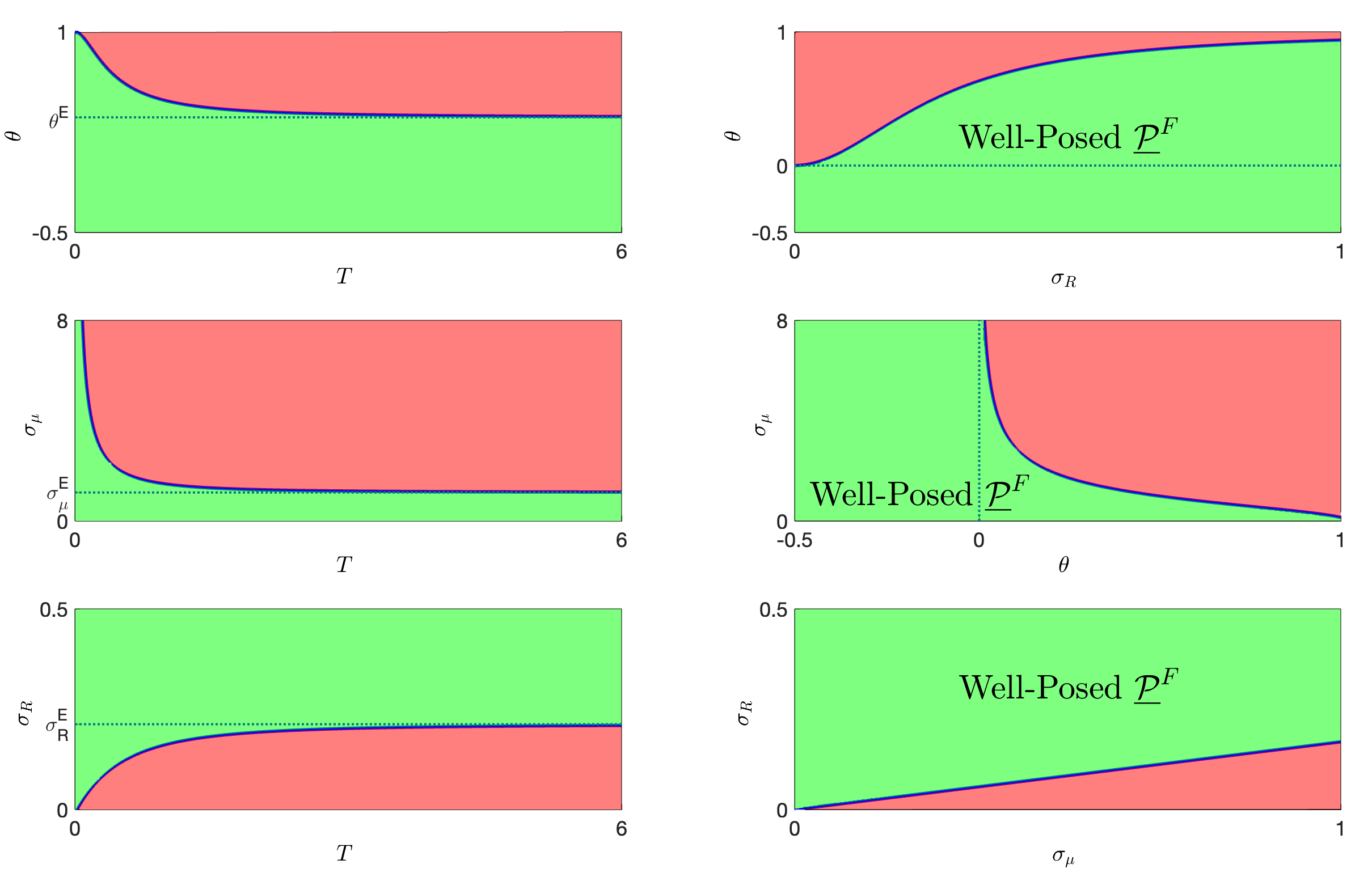
Figure 1: Subset $\underline{\pazocal P}^{F}$ of the set of feasible parameters $\pazocal P^{F}$
depending on   $\theta~{}~{}$ and $T$ (top left),       $\theta$ and $\sigma_{R}$ (top right),
depending on   $\sigma_{\mu}$ and $T$ (middle left), $\sigma_{\mu}$ and $\theta$   (middle right),
depending on   $\sigma_{R}$ and $T$ (bottom left), $\sigma_{R}$ and $\sigma_{\mu}$ (bottom right).
The other parameters are given in Table 1.

In Section 3 we have specified sufficient conditions to the model parameters for which the optimization problem is well-posed. For market models with a single risky asset which is assumed for the numerical experiments these conditions are given Corollary 3.9. In Figure 1 we visualize the subset $\underline{\pazocal P}^{F}$ of the set of feasible parameters $\pazocal P^{F}$ for which well posedness for the utility maximization problem of the fully informed investor can be guaranteed. In particular, we show the dependence of $\pazocal P^{F}$ on the investment horizon $T$, the power utility parameter $\theta$, the volatility $\sigma_{\mu}$ of the drift and the volatility $\sigma_{R}$ of the stock price.

The two top panels show the subset $\underline{\pazocal P}^{F}$ depending on $\theta,T$ and $\sigma_{R}$. It can be seen that for negative $\theta$, i.e. for investors which are more risk averse than the log-utility investor, the optimization problem is always well-posed. Moreover, the top left panel shows that for the selected parameters the optimization problem is well-posed for all $T>0$ if the parameter $\theta$ does not exceed the critical value $\theta^{E}\approx 0.36$. For $\theta>\theta^{E}$, i.e. for investors with sufficiently small risk-aversion, the optimization problem is no longer well-posed for all investment horizons $T$, but only up to a critical investment horizon $T^{E}=T^{E}(\theta)$ depending on $\theta$ and given in (27). The larger $\theta$, the smaller is that critical investment horizon $T(\theta)$. For the limiting case $\theta\rightarrow 1$ it holds $T^{E}(\theta)\rightarrow 0$. The top right panel shows for an investment horizon fixed to $T=1$ the subset $\underline{\pazocal P}^{F}$ depending on $\theta$ volatility $\sigma_{R}$ of stock price. It can be seen that larger values for the stock volatility allow to choose larger values of $\theta$.

The two panels in the middle illustrate the influence of the drift volatility $\sigma_{\mu}$ on the subset $\underline{\pazocal P}^{F}$ . The left panel shows that the optimization problem is well-posed for all $T>0$ as long as the volatility $\sigma_{\mu}$ of the drift does not exceed the critical value $\sigma_{\mu}^{E}\approx 1.15$. For volatilities $\sigma_{\mu}>\sigma_{\mu}^{E}$ the optimization problem is well-posed only for investment horizons $T$ smaller than the critical horizon $T^{E}=T^{E}(\sigma_{\mu})$ that depends on $\sigma_{\mu}$ and is given in (27).

In the right panel we investigate for fixed investment horizon $T=1$ the dependence of $\pazocal P^{F}$ on the drift volatility $\sigma_{\mu}$ and the power utility parameter $\theta$. While for $\theta<0$ there are no further restrictions on the parameters, this is no longer true for $\theta\in(0,1)$. The larger the volatility $\sigma_{\mu}$ the smaller one has to choose $\theta$.

The bottom two panels illustrate the influence of stock volatility $\sigma_{R}$ on the subset $\underline{\pazocal P}^{F}$ . In contrast to the volatility $\sigma_{\mu}$ of the drift, smaller values of $\sigma_{R}$ imply that the optimization problem is well-posed only for smaller $T$ as it can be seen in the bottom left panel. If $\sigma_{R}$ does not exceed the critical value $\sigma_{R}^{E}\approx 0.22$, then the optimization problem is well-posed only up to a critical investment horizon $T^{E}=T^{E}(\sigma_{R})$ that depends on $\sigma_{R}$. The larger $\sigma_{R}$, the larger the horizon can be set. However, for $\sigma_{R}$ exceeding the critical value $\sigma_{R}^{E}$ the control problem is well defined for any horizon time $T>0$. The bottom right panel shows the dependence of $\pazocal P^{F}$ on the two volatilities $\sigma_{R}$ and $\sigma_{\mu}$. Note that the two regions are separated by a straight line as it can be deduced from (26) and (27).

Finally, we consider the case of a partial informed investor. Then an additional condition on the covariance process $Q^{H}$ of the filter has to imposed to ensure well posedness. We refer to Corollary 3.7 for the multi-dimensional case and to Corollary 3.9 and (29) for the special case of markets with a single risky asset considered above. Here, the sufficient condition requires that $Q^{H}_{t}<1/(2A_{\gamma}(t))$ which is satisfied for the the model parameters from Table 1. First, it is known that $A_{\gamma}$ is decreasing on $[0,T]$. Second, properties of the conditional covariance process (see Gabih et al (2022) PowerFixed ; Sass et al (2017) ; Sass et al (2021) ) imply $Q^{H}_{t}\leq Q^{R}_{t}$. Further, for $q_{0}>Q_{\infty}^{R}=\lim_{t\to\infty}Q_{t}^{R}$ we have that $Q^{R}$ is decreasing. Here, it holds $Q_{\infty}^{R}<q_{0}$, thus we have $Q^{H}_{t}\leq q_{0}=0.1\overline{6}<0.675=\frac{1}{2A_{\gamma}(0)}\leq\frac{1}{2A_{\gamma}(t)}$ which shows that the problem is well-posed.

Appendix A Proof of Lemma 3.2

Proof

Consider first the function $D\in\pazocal C^{1,2}$ defined as follows

$${D}:[0,T]\times\mathbb{R}^{+}\times\mathbb{R}^{d}\rightarrow\mathbb{R}_{+};\qquad{D}(t,z,m):={\mathbb{E}}\left[\Psi_{T}^{t,z,m}\right].$$ (30)

Then it holds ${D}(T,z,m)={\mathbb{E}}\left[\xi_{T}^{T,z,m}\right]={\mathbb{E}}\left[z\right]=z$.
The dynamics of the drift $\mu$ and the process $\Psi$ for $s\in[t,T]$ read as

$$\begin{pmatrix}d\mu_{s}^{t,m}\\ d\Psi_{s}^{t,z,m}\end{pmatrix}=\begin{pmatrix}\kappa(\overline{\mu}-\mu_{s}^{t,m})\\ \gamma\Psi_{s}^{t,z,m}\big{(}\mu_{s}^{t,m}\big{)}^{\top}\Sigma_{R}^{-1}\mu_{s}^{t,m}\end{pmatrix}ds+\begin{pmatrix}\sigma_{\mu}\\ {0}_{1\times d_{2}}\end{pmatrix}dW_{s}^{\mu};\quad\begin{pmatrix}\mu_{t}^{t,m}\\ \Psi_{t}^{t,z,m}\end{pmatrix}=\begin{pmatrix}m\\ z\end{pmatrix}.$$

The drift and the diffusion coefficients of the last equation satisfy the Lipschitz- and linear growth conditions. Moreover, the Feynman-Kac-Formula for the expectation from (30) leads to the following partial differential equation for ${D}$

$$0=\frac{\partial}{\partial t}{D}(t,z,m)+\nabla_{m}^{\top}{D}(t,z,m)\;\kappa(\overline{\mu}-m) +\frac{1}{2}tr\{\nabla_{mm}{D}(t,z,m)\Sigma_{\mu}\}+\gamma zm^{\top}\Sigma_{R}^{-1}m\frac{\partial G_{b}(t,z,m)}{\partial z}$$ (31)

with ${D}(T,z,m)=z$ as terminal condition. The above terminal value problem can be solved with the following separation ansatz

$${D}(t,z,m)=z\;d(t,m),\quad d(T,m)=1.$$ (32)

At time $t$ we have $\mu_{t}^{t,m}=m$ and $\Psi_{t}^{t,1,m}=1$ so that we obtain ${\mathbb{E}}\big{[}\Psi_{T}^{t,1,m}\big{]}={D}(t,1,m)=d(t,m)$ which is the function $d$ defined in Lemma (3.2). Plugging (32) into (31) leads to the following linear parabolic PDE for $d$

$$0=\frac{\partial}{\partial t}d(t,m)+\nabla_{m}^{\top}d(t,m)\;\kappa(\overline{\mu}-m) +\frac{1}{2}tr\{\nabla_{mm}d(t,m)\Sigma_{\mu}\}+\gamma m^{\top}\Sigma_{R}^{-1}m\;d(t,m)$$

with terminal value $d(T,m)=1$. For solving the above PDE the ansatz

$$d(t,m)=\exp\big{\{}m^{\top}A_{\gamma}(t)m+B_{\gamma}^{\top}(t)m+C_{\gamma}(t)\big{\}}.$$

leads to the system of ODEs for $A_{\gamma}$, $B_{\gamma}$ and $C_{\gamma}$, which are given in (16), (17) and (18).

Appendix B Proof of Theorem 3.3

Proof

In the proof we follow an approach presented in Angoshtari (Angoshtari2013, , Theorem 1.8). Let $(\xi_{t})_{t\in[0,T]}$ be a stochastic process satisfying the SDE

$$d\xi_{t}={\color[rgb]{1,0,0}{-}}\xi_{t}\mu_{t}^{\top}\;\Sigma_{R}^{-1}\sigma_{R}\;dW_{t}^{R},\quad\xi_{0}=1,\;~{}\mu_{0}=\overline{m}_{0},$$ (33)

with the solution

$$\xi_{t}=\exp\Big{\{}-\frac{1}{2}\int\nolimits_{0}^{t}\|\mu_{s}^{\top}\;\Sigma_{R}^{-1}\sigma_{R}\|^{2}ds-\int\nolimits_{0}^{t}\mu_{s}^{\top}\;\Sigma_{R}^{-1}\sigma_{R}\;dW_{s}^{R}\Big{\}}.$$ (34)

For $t_{0}\in[0,T]$ we denote by $\mu_{t}^{t_{0},\overline{m}}$ the solution to the drift equation (3) starting at time $t_{0}$ with initial value $\overline{m}$, by $X_{t}^{\pi,t_{0},x,\overline{m}}$ the solution to the wealth equation (6) with initial values $(x,\overline{m})$ and by $\xi_{t}^{t_{0},z,\overline{m}}$ the solution of (33) at time $t$ with initial values $(z,\overline{m})$. Applying Itô’s-formula it holds

$$d(X^{\pi,0,x,\overline{m}_{0}}~{}\xi^{0,1,\overline{m}_{0}})_{t} =X_{t}^{\pi,0,x,\overline{m}_{0}}~{}d\xi_{t}^{0,1,\overline{m}_{0}}+\xi_{t}^{0,1,\overline{m}_{0}}\;dX_{t}^{\pi,0,x,\overline{m}_{0}}+d\langle X^{\pi,0,x,\overline{m}_{0}},\xi^{0,1,\overline{m}_{0}}\rangle_{t}$$

$$=\xi_{t}^{0,1,\overline{m}_{0}}~{}X_{t}^{\pi,0,x,\overline{m}_{0}}[\pi_{t}^{\top}\sigma_{R}-\mu_{t}^{0,\overline{m}_{0}}\Sigma_{R}^{-1}\sigma_{R}]\;dW_{t}^{R}.$$ (35)

Moreover, Fatou’s Lemma implies that the non-negative process $(X^{\pi}\xi)_{t}$ is a supermartingal, and as consequence it holds

$$x-{\mathbb{E}}[X_{T}^{\pi,0,x,\overline{m}_{0}}~{}\xi_{T}^{0,1,\overline{m}_{0}}]\geq 0.$$ (36)

From the other hand let $f:\mathbb{R}^{+}\rightarrow\mathbb{R}$ be the associated Legendre-Fenchel-Transformation of the utility function $\pazocal U_{\theta}(x)$ defined for every $w>0$ by

$$f(w):=\sup\limits_{x\in\mathbb{R}^{+}}\left\{\pazocal U_{\theta}(x)-xw\right\}=\frac{1-\theta}{\theta}w^{-\frac{\theta}{1-\theta}}.$$ (37)

Since $\xi_{T}^{0,1,\overline{m}_{0}}>0$, it holds for every $w>0$

$$f(\xi_{T}^{0,1,\overline{m}_{0}}~{}w)=\sup\limits_{x\in\mathbb{R}^{+}}\Big{\{}\pazocal U_{\theta}(x)-x\;\xi_{T}^{0,1,\overline{m}_{0}}\;w\Big{\}}\geq\pazocal U_{\theta}(X_{T}^{\pi,0,x,\overline{m}_{0}})-X_{T}^{\pi,0,x,\overline{m}_{0}}\;\xi_{T}^{0,1,\overline{m}_{0}}\;w.$$ (38)

Now for $w>0$ inequality (36) implies that

$${\mathbb{E}}\big{[}\pazocal U_{\theta}(X_{T}^{\pi,0,x,\overline{m}_{0}})\big{]} \leq{\mathbb{E}}\big{[}\pazocal U_{\theta}(X_{T}^{\pi,0,x,\overline{m}_{0}})\big{]}+w\big{(}x-{\mathbb{E}}\big{[}X_{T}^{\pi,0,x,\overline{m}_{0}}~{}\xi_{T}^{0,1,\overline{m}_{0}}\big{]}\big{)}$$

$$={\mathbb{E}}\big{[}\pazocal U_{\theta}(X_{T}^{\pi,0,x,\overline{m}_{0}})-X_{T}^{\pi,0,x,\overline{m}_{0}}\;\xi_{T}^{0,1,\overline{m}_{0}}\;\text{$w$}\big{]}+xw$$

$$\leq{\mathbb{E}}\Big{[}f(\xi_{T}^{0,1,\overline{m}_{0}}~{}w)\Big{]}+x\text{$w$},$$

where the last inequality follows from (38). For the term $f(\xi_{T}^{0,1,\overline{m}_{0}}~{}w)$ we now apply (37) to obtain

$${\mathbb{E}}\big{[}\pazocal U_{\theta}(X_{T}^{\pi,0,x,\overline{m}_{0}})\big{]} \leq\frac{1-\theta}{\theta}w^{-\frac{\theta}{1-\theta}}{\mathbb{E}}\big{[}\big{(}\xi_{T}^{0,1,\overline{m}_{0}}\big{)}^{-\frac{\theta}{1-\theta}}\big{]}+xw.$$ (39)

Since the last inequality holds for every admissible strategy $\pi\in\pazocal A^{G}$ and for every $w>0$, we can take the supremum over all strategies $\pi\in\pazocal A^{G}$ on the left-hand side and the infimum over all $w>0$ in the right-hand side to obtain

$$\pazocal V_{0}^{G}=\sup\limits_{\pi\in\pazocal A^{G}}{\mathbb{E}}\big{[}\pazocal U_{\theta}(X_{T}^{\pi,0,x,\overline{m}_{0}})\big{]} \leq\frac{1}{\theta}x^{\theta}\ \big{(}{\mathbb{E}}\big{[}\big{(}\xi_{T}^{0,1,\overline{m}_{0}}\big{)}^{-\frac{\theta}{1-\theta}}\big{]}\big{)}^{1-\theta}.$$ (40)

The problem is now reduced to investigate if the expectation in the r.h.s. of (40) is bounded. It holds

$$\big{(}\xi_{T}^{0,1,m}\big{)}^{-\frac{\theta}{1-\theta}} =\exp\Big{\{}\frac{\theta}{1-\theta}\Big{(}\frac{1}{2}\int\nolimits_{0}^{T}\big{\|}\big{(}\mu_{s}^{0,m}\big{)}^{\top}\Sigma_{R}^{-1}\sigma_{R}\big{\|}^{2}\;ds+\int\nolimits_{0}^{T}\big{(}\mu_{s}^{0,m}\big{)}^{\top}\Sigma_{R}^{-1}\sigma_{R}\;dW_{s}^{R}\Big{)}\Big{\}}=\Lambda_{T}\cdot\Psi_{T}^{0,1,m},$$

where $\Psi_{T}^{0,1,m}$ is given in (14) with $\gamma=\frac{\theta}{2(1-\theta)^{2}}$, and the term $\Lambda_{T}$ is given by

$$\Lambda_{T}=\exp\Big{\{}\int\nolimits_{0}^{T}\frac{\theta}{1-\theta}\big{(}\mu_{s}^{0,m}\big{)}^{\top}\Sigma_{R}^{-1}\sigma_{R}\;dW_{s}^{R}-\frac{1}{2}\int\nolimits_{0}^{T}\big{\|}\frac{\theta}{1-\theta}\big{(}\mu_{s}^{0,m}\big{)}^{\top}\Sigma_{R}^{-1}\sigma_{R}\big{\|}^{2}\;ds\bigg{\}}.$$

We now introduce a new probability measure  $P^{\ast}$ given by $\frac{dP^{\ast}}{dP~{}}=\Lambda_{T}$ so that the expectation from (40) can be expressed as follows

$${\mathbb{E}}\Big{[}\big{(}\xi_{T}^{0,1,m}\big{)}^{\frac{-\theta}{1-\theta}}\big{]} ={\mathbb{E}}\big{[}\Lambda_{T}\cdot\Psi_{T}^{0,1,m}\big{]}={\mathbb{E}}^{\ast}\Big{[}\Psi_{T}^{0,1,m}\Big{]}=d(0,m).$$

This expectation can be expressed according to (15) in Lemma 3.2, where ${\mathbb{E}}^{\ast}$ denotes the expectation under the new probability measure.

Appendix C Proof of Lemma 3.5

Proof

We give the proof for an invertible matrix $\Sigma_{Y}$. The general case is similar. It holds

$${\mathbb{E}}\big{[}\exp\big{\{}(Y+{b})^{\top}{U}(Y+{b})\big{\}}\big{]} =\big{(}(2\pi)^{d}\rm{det}(\Sigma_{Y})\big{)}^{-1/2}\int\nolimits_{\mathbb{R}^{d}}\exp\{f_{Y}(y)\}dy$$ (41)

with $f_{Y}(y):=-\frac{1}{2}(y-\mu_{Y})^{\top}\Sigma_{Y}^{-1}(y-\mu_{Y})+(y+{b})^{\top}{U}(y+{b})$. Quadratic complement with respect to $y$ with the notation $\Sigma_{Z}:=(\Sigma_{Y}^{-1}-2{U})^{-1}$ and $\mu_{Z}:=\Sigma_{Z}(2{U}{b}+\Sigma_{Y}^{-1}\mu_{Y})$ yields

$$f_{Y}(y) =-\frac{1}{2}(y-\mu_{Z})^{\top}\;\Sigma_{Z}^{-1}\;(y-\mu_{Z})+\frac{1}{2}\mu_{Z}^{\top}\Sigma_{Z}^{-1}\mu_{Z}+{b}^{\top}{U}{b}-\frac{1}{2}\mu_{Y}^{\top}\Sigma_{Y}^{-1}\mu_{Y}$$

$$=-\frac{1}{2}(y-\mu_{Z})^{\top}\;\Sigma_{Z}^{-1}\;(y-\mu_{Z})+(\mu_{Y}+{b})^{\top}\;({I}_{d}-2{U}\Sigma_{Y})^{-1}{U}(\mu_{Y}+{b}).$$ (42)

Substituting (42) into (41) and using that for a Gaussian random vector $Z\sim\pazocal N(\mu_{Z},\Sigma_{Z})$ the probability density function is $f_{Z}(y)=\big{(}(2\pi)^{d}\rm{det}(\Sigma_{Z})\big{)}^{-1/2}\exp\{-\frac{1}{2}(y-\mu_{Z})^{\top}\;\Sigma_{Z}^{-1}\;(x-\mu_{Z})\}$ with $\int_{\mathbb{R}^{d}}f_{Z}(x)\,dx=1$ and the relation $(\rm{det}(\Sigma_{Z})^{1/2}\rm{det}(\Sigma_{Y})^{-1/2}=(\rm{det}(\Sigma_{Y}^{-1}-2{U})\rm{det}(\Sigma_{Y}))^{-1/2}=(\rm{det}(I_{d}-2{U}\Sigma_{Y}))^{-1/2}$ proves the assertion.

Appendix D Proof of Theorem 3.6

Proof

We recall (20) stating $\pazocal V_{0}^{H}(\varrho)\leq\frac{x_{0}^{\theta}}{\theta}{\mathbb{E}}[d(0,\mu_{0})|\pazocal F_{0}^{H}]$. For the $H$-investors with $H=R,J,Z$ the conditional distribution of $\mu_{0}$ given $\pazocal F_{0}^{H}$ is the Gaussian distribution $\pazocal N(m_{0},q_{0})$. Thus we can write the conditional expectation ${\mathbb{E}}[d(0,\mu_{0})|\pazocal F_{0}^{H}]$ as ${\mathbb{E}}\big{[}d(0,m_{0}+q_{0}^{1/2}\varepsilon)\big{]}$ with a random variable $~{}\varepsilon\sim\pazocal N(0,I_{d})$ independent of $\pazocal F_{0}^{H}$. To simplify the notation we write in the following $A,B,C$ instead of $A_{\gamma}(0),B_{\gamma}(0),C_{\gamma}(0)$, respectively. Substituting into (20) and using representation (15) we deduce

$${\mathbb{E}}[d(0,\mu_{0})|\pazocal F_{0}^{H}] ={\mathbb{E}}\big{[}d(0,m_{0}+q_{0}^{1/2}\varepsilon)\big{]}$$

$$={\mathbb{E}}\big{[}\exp\big{\{}(m_{0}+{q_{0}}^{1/2}\varepsilon)^{\top}A(m_{0}+{q_{0}}^{1/2}\varepsilon)+B^{\top}(m_{0}+{q_{0}}^{1/2}\varepsilon)+C\big{\}}\big{]}$$

$$={\mathbb{E}}\big{[}\exp\big{\{}m_{0}^{\top}Am_{0}+B^{\top}m_{0}+C\big{\}}\exp\big{\{}({q_{0}}^{1/2}\varepsilon)^{\top}A{q_{0}}^{1/2}\varepsilon+(2m_{0}^{\top}A+B^{\top}){q_{0}}^{1/2}\varepsilon\big{\}}\big{]}$$

$$=d(0,m_{0}){\mathbb{E}}\big{[}\exp\big{\{}({q_{0}}^{1/2}\varepsilon)^{\top}A{q_{0}}^{1/2}\varepsilon+(2Am_{0}+B)^{\top}{q_{0}}^{1/2}\varepsilon\big{\}}\big{]}$$

$$=d(0,m_{0})\exp\Big{\{}-\frac{1}{4}{a}^{\top}A^{-1}{a}\Big{\}}{\mathbb{E}}\big{[}\exp\{Y^{\top}{A}Y\}\big{]}$$ (43)

where $Y=q_{0}^{1/2}\varepsilon+\frac{1}{2}A^{-1}a\sim\pazocal{N}(\mu_{Y},\Sigma_{Y})$ is a Gaussian random vector with mean $\mu_{Y}=\frac{1}{2}A^{-1}a$ and covariance matrix $\Sigma_{Y}=q_{0}$. We recall that $a=2Am_{0}+B$ and ${K}=I_{d}-2Aq_{0}$. Applying Lemma 3.5 with ${U}=A$ and ${b}=0_{d}$ yields

$${\mathbb{E}}\big{[}\exp\{Y^{\top}{A}Y\}\big{]} =\big{(}\rm{det}(K)\big{)}^{-1/2}\exp\big{\{}\mu_{Y}^{\top}\;K^{-1}A\,\mu_{Y}\big{\}}$$

and we obtain from (43)

$${\mathbb{E}}[d(0,\mu_{0})|\pazocal F_{0}^{H}] =d(0,m_{0})\big{(}\rm{det}(K)\big{)}^{-1/2}\exp\Big{\{}\mu_{Y}^{\top}\;K^{-1}A\,\mu_{Y}-\frac{1}{4}{a}^{\top}A^{-1}{a}\Big{\}}$$ (44)

Rearranging terms in the exponent using the symmetry of $A$ yields

$$\mu_{Y}^{\top}\;K^{-1}A\,\mu_{Y}-\frac{1}{4}{a}^{\top}A^{-1}{a} =\frac{1}{4}{a}^{\top}A^{-1}K^{-1}\,{a}-\frac{1}{4}d^{\top}A^{-1}d$$

$$=\frac{1}{4}{a}^{\top}A^{-1}\big{(}I_{d\times d}-K\big{)}K^{-1}\,{a}=\frac{1}{4}{a}^{\top}A^{-1}2Aq_{0}K^{-1}\,{a}=\frac{1}{2}{a}^{\top}q_{0}K^{-1}\,{a}.$$

Substituting into (44) and (20) proves the claim.

References

- (1) Angoshtari, B. (2014): Stochastic Modeling and Methods for Portfolio Managment in Cointegrated Markets. PhD thesis, University of Oxford, https://ora.ox.ac.uk/objects/uuid:1ae9236c-4bf0-4d9b-a694-f08e1b8713c0
- (2) Angoshtari, B. (2016): Portfolio On the Market-Neutrality of Optimal Pairs-Trading Strategies. arXiv:1608.08268 [q-fin.PM].
- (3) Battauz, A., De Donno, M. and Sbuelz, A. (2017): Reaching Nirvana With a Defaultable Asset?. Decisions in Economics and Finance 40, 31–52.
- (4) Björk, T., Davis, M. H. A. and Landén, C. (2010): Optimal Investment with Partial Information, Mathematical Methods of Operations Research 71, 371–399.
- (5) Black, F. and Litterman, R. (1992): Global Portfolio Optimization. Financial Analysts Journal 48(5), 28-43.
- (6) Brendle, S. (2006): Portfolio Selection Under Incomplete Information. Stochastic Processes and their Applications, 116(5), 701-723.
- (7) Chen, K. and Wong, Y. (2022): Duality in optimal consumption–investment problems with alternative data. arXiv:2210.08422 [q-fin.MF].
- (8) Colaneri, K., Herzel, S. and Nicolosi, M. (2021): The Value of Knowing the Market Price of Risk. Annals of Operations Research 299, 101–131.
- (9) Davis, M. and Lleo, S. (2013): Black-Litterman in Continuous Time: the Case for Filtering. Quantitative Finance Letters, 1,30-35
- (10) Davis, M. and Lleo, S. (2020): Debiased Expert Opinions in Continuous Time Asset Allocation. Journal of Banking & Finance, Vol. 113, 105759.
- (11) Davis, M. and Lleo, S. (2022): Jump-diffusion risk-sensitive benchmarked asset management with traditional and alternative data. Annals of Operations Research. DOI:10.1007/s10479-022-05130-3
- (12) Fleming, W. and Rishel, R.: Deterministic and Stochastic Optimal Control , Springer New York (1975).
- (13) Fouque, J. P, Papanicolaou, A. and Sircar, R. (2015): Filtering and Portfolio Optimization with Stochastic Unobserved Drift in Asset Returns. SSRN Electronic Journal,13(4):935-953.
- (14) Frey, R., Gabih, A. and Wunderlich, R. (2012): Portfolio Optimization under Partial Information with Expert Opinions. International Journal of Theoretical and Applied Finance, 15, No. 1.
- (15) Frey, R., Gabih, A. and Wunderlich, R. (2014): Portfolio Optimization under Partial Information with Expert Opinions: Dynamic Programming Approach. Communications on Stochastic Analysis Vol. 8, No. 1 (2014) 49-71.
- (16) Gabih, A., Kondakji, H. Sass, J. and Wunderlich, R. (2014): Expert Opinions and Logarithmic Utility Maximization in a Market with Gaussian Drift. Communications on Stochastic Analysis Vol. 8, No. 1 (2014) 27-47.
- (17) Gabih, A., Kondakji, H. and Wunderlich, R. (2020): Asymptotic Filter Behavior for High-Frequency Expert Opinions in a Market with Gaussian Drift. Stochastic Models 36:4, 519-547, 2020.
- (18) Gabih, A., Kondakji, H. and Wunderlich, R. (2023): Power Utility Maximization with Expert Opinions at Fixed Arrival Times in a Market with Hidden Gaussian Drift. arXiv:2301.06847 [q-fin.PM]
- (19) Gabih, A. and Wunderlich, R.: Portfolio optimization in a market with hidden Gaussian drift and randomly arriving expert opinions: Modeling and theoretical results. arXiv:2308.02049 [q-fin.PM] (2023).
- (20) Kim, T. S. and Omberg, E. (1996): Dynamic Nonmyopic Portfolio Behavior, The Review of Financial Studies 9(1), 141-161.
- (21) Kondakji, H. (2019): Optimal Portfolios for Partially Informed Investors in a Financial Market with Gaussian Drift and Expert Opinions (in German). PhD Thesis BTU Cottbus-Senftenberg. Available at https://opus4.kobv.de/opus4-btu/frontdoor/deliver/index/docId/4736/file/Kondakji_Hakam.pdf
- (22) Korn, R. and Kraft, H. (2004): On the Stability of Continuous-Time Portfolio Problems with Stochastic Opportunity Set, Mathematical Finance 14(3), 403-414.
- (23) Lakner, P. (1998): Optimal Trading Strategy for an Investor: The Case of Partial Information. Stochastic Processes and their Applications 76, 77-97.
- (24) Lee, S. and Papanicolaou A.: Pairs trading of two assets with uncertainty in co-integration’s level of mean reversion. International Journal of Theoretical and Applied Finance 19 (08), 1650054 (2016)
- (25) Rieder, U. and Bäuerle, N. (2005): Portfolio Optimization with Unobservable Markov-Modulated Drift Process. Journal of Applied Probability 43, 362-378.
- (26) Roduner, Ch.: Die Riccati-Gleichung, IMRT-Report Nr. 26, ETH Zurich (1994).
- (27) Rogers, L.C.G.(2013): Optimal Investment. Briefs in Quantitative Finance. Springer, Berlin-Heidelberg.
- (28) Sass, J. and Haussmann, U.G (2004): Optimizing the Terminal Wealth under Partial Information: The Drift Process as a Continuous Time Markov Chain. Finance and Stochastics 8, 553-577.
- (29) Sass, J., Westphal, D. and Wunderlich, R. (2017): Expert Opinions and Logarithmic Utility Maximization for Multivariate Stock Returns with Gaussian Drift. International Journal of Theoretical and Applied Finance Vol. 20, No. 4, 1-41.
- (30) Sass, J., Westphal, D. and Wunderlich, R. (2021): Diffusion Approximations for Randomly Arriving Expert Opinions in a Financial Market with Gaussian Drift. Journal of Applied Probability, 58 (1), 197 - 216.
- (31) Sass, J., Westphal, D. and Wunderlich, R. (2022): Diffusion approximations for periodically arriving expert opinions in a financial market with Gaussian drift. Stochastic Models, DOI:10.1080/15326349.2022.2100423
- (32) Schöttle, K., Werner, R. and Zagst, R. (2010): Comparison and Robustification of Bayes and Black-Litterman Models. Mathematical Methods of Operations Research 71, 453–475.