Bagged Polynomial Regression and Neural Networks

Abstract

Series and polynomial regression are able to approximate the same function classes as neural networks. However, these methods are rarely used in practice, although they offer more interpretability than neural networks. In this paper, we show that a potential reason for this is the slow convergence rate of polynomial regression estimators and propose the use of bagged polynomial regression (BPR) as an attractive alternative to neural networks. Theoretically, we derive new finite sample and asymptotic $L^{2}$ convergence rates for series estimators. We show that the rates can be improved in smooth settings by splitting the feature space and generating polynomial features separately for each partition. Empirically, we show that our proposed estimator, the BPR, can perform as well as more complex models with more parameters. Our estimator also performs close to state-of-the-art prediction methods in the benchmark MNIST handwritten digit dataset.

1 Introduction

Deep learning models have become ubiquitous in the machine learning literature. A cornerstone of the success of deep neural networks is that they can over-fit the training data while maintaining excellent generalization error. This feat is possible by training very large (over-parametrized) models with methods that induce self-regularization. At the same time, an extensive literature on universal approximators (starting with [7] and [10] among others) suggests that most neural network architectures can approximate the same function classes as polynomial regression models. In fact, polynomial regression approximations are used to study the generalization capacities of neural networks, for example, recently in [8] in a student/teacher model. In light of this, a question arises: why is polynomial regression not used more often in practice for predictive tasks?

One of the main reasons is that the number of transformed features in polynomial regression models increases exponentially with the dimension of the feature space and the degree of the polynomial embedding. This large number of features leads to two important problems in practice: (1) computationally, the model becomes very expensive very fast, and (2) the finite sample rates for the $L^{2}$ estimation error may require a prohibitively large sample size (i.e., slow convergence). Together these two problems imply that even in big data settings with access to computational power, it may be unfeasible to use polynomial regression for predictive tasks. Besides explicit regularization (shrinkage through penalty terms), some of the frequently suggested solutions to this problem include (1) embedding/dimensionality reduction, for example, by using PCA or by extracting an auto-encoder embedding [12]; (2) constraining the feature map, for instance for image data by adding a convolution step in generating the features [13], or (3) model ensembling, for example by bagging models [3].

In this paper, we focus on the second solution by showing theoretically how constraining the feature map in series regression affects the finite sample rate of the learning problem and proposing the use of a more flexible estimator, the bagged polynomial regression (BPR). Our theoretical contribution is characterizing a class of series regression models for which the $L^{2}$ finite sample rate for the learning problem can be optimized by building the polynomial features group-wise for a partition of the feature space rather than for all features. Intuitively, our theoretical results show how partitioning the feature space can optimally trade off the estimation and approximation errors to improve the rate of convergence and, therefore, the prediction error. These results are especially useful for smooth dense cases (not sparse) in which good models need to include high-order interactions to achieve a good fit.

Drawing from the theoretical insights, we propose the use of BPR as an alternative to neural networks that is computationally attractive and readily implementable in most machine learning software packages. By only building the polynomial embeddings for subsets of the feature space and averaging across multiple models, BPR can reduce the number of parameters needed to estimate models while maintaining low prediction and generalization errors. We analyze the performance of BPR in a standard prediction task to the MNIST hand-written digit database [14]. Our application shows that training BPR using only a fraction of the available features in each estimator performs comparably well to larger models. Furthermore, BPR performs better than standard polynomial regressions and achieves a test accuracy on MNIST close to convolutional neural networks and state-of-the-art methods. We believe that a fully tuned BPR model could perform like state-of-the-art in standard prediction tasks.

Related Literature On the theoretical side, this paper is mostly related with the series regression literature (see for example [15]) and the non-parametric regression literature (see for example [19]). Our paper builds on [2] by using [17] to get new asymptotic $L^{2}$ rates and then provides new finite sample rates for series regression models. Then, it uses these results to show that the rates can be optimized for partitioned series regression models. Theoretical treatments of similar partitioning models have been explored in the literature, for example [1] for additive interactive regression models, [5] for partitioning estimators or more recently [11] on sub-sampling ensembling in high dimensions. Our results can complement this literature by providing new finite sample rates for a related but different class of models. This paper may also be of interest to the machine learning literature regarding universal approximators for neural networks and polynomial regression and complement the recent literature comparing the two models, for example, [8] or [6]. In particular, our results improve on the [8] finding that polynomial regression can perform comparably well to neural networks.

Notation In what follows we use $E$ to denote the expectation operator and $\mathbb{E}$ to denote the empirical expectation operator such that $\mathbb{E}_{n}[f(x)]=1/n\sum_{i=1}^{n}f(x_{i})$. Furthermore, unless stated otherwise we denote the $l_{2}$ norm for a vector by $\|\cdot\|$, the operator norm for a matrix $\|\cdot\|_{op}$ and let $a\lor b=\max\{a,b\}$. Finally, we write $a\lesssim b$ to mean $a\leq Cb$ for some fixed constant $C>0$, $a\lesssim_{P}b$ to mean $a=O_{p}(b)$ and $a\asymp b$ to mean $a$ is asymptotic to $b$. All proofs can be found in the supplementary material appendix.

2 Theoretical results

We derive asymptotic and finite sample rates for sequences of models indexed by sample size $n$ that satisfy the following sampling assumption.

A. 1 (Sampling model).

For each $n$, random vectors $\{(y_{i},x_{i}^{\prime})\}_{i=1}^{n}$ are $i.i.d$ and given by the series regression model

$$y_{i}=g(x_{i})+\epsilon_{i},\quad E[\epsilon_{i}|x_{i}]=0,\quad x_{i}\in\mathcal{X}\subset\mathbb{R}^{d},\quad i=1,\dots,n,$$ (1)

where $y_{i}\in\mathbb{R}$ is the response variable, $x_{i}$ are the basic features in some bounded set $\mathcal{X}$, $\epsilon_{i}$ is a noise term and $g:\mathcal{X}\to\mathbb{R}$ is the conditional expectation function belonging to an arbitrary function class $\mathcal{G}$.

Given the sampling process, we focus on the set of models in which $g$ is approximated by linear forms $p(x)^{\prime}b$, where $p(x):\mathbb{R}^{d}\to\mathbb{R}^{k}$ is a tensor operator that generates polynomial features, with $k$ being the total number of features generated from the basic features $x$. For an iid sample $\{y_{i},x_{i}^{\prime}\}$, $i=1,\dots,n$, we estimate the series regressors by the minimizing the statistical risk for the square loss function (i.e. the least squares problem):

$$\beta_{g}=\text{argmin}_{b\in\mathbb{R}^{k}}E[(g(x_{i})-p(x_{i})^{\prime}b)^{2}],$$ (2)

where $\beta_{g}$ is the least squares estimate for a given conditional mean function $g$. This set up follows the set up in [2] and the standard framework in the series regression literature (see [15] or [1]). A key object in this literature is the approximation error $r_{g}(x)$ for features $x$ and target function $g$, defined as

$$r_{g}(x)=g(x)-p(x)^{\prime}\beta_{g}.$$ (3)

We can then re-write the sampling model as linear regression model

$$y_{i}=p_{i}^{\prime}\beta+u_{i},\quad E[u_{i}x_{i}]=0,\quad u_{i}=r_{i}+\epsilon_{i},$$ (4)

and define the standard least squares projection estimator:

$$\hat{\beta}=\text{argmin}_{b\in\mathbb{R}^{k}}\mathbb{E}_{n}[(y_{i}-p_{i}^{\prime}b)^{2}]=\mathbb{E}_{n}[p_{i}p_{i}^{\prime}]^{-1}\mathbb{E}_{n}[p_{i}y_{i}].$$ (5)

Given the regression model we can decompose the error in estimating the target function $g(x)$ in two components, an estimation error and an approximation error

$$\hat{g}(x)-g(x)=\underbrace{p(x)^{\prime}(\hat{\beta}-\beta)}_{\text{estimation error}}\quad-\underbrace{r(x).}_{\text{approximation error}}$$ (6)

Intuitively, the richer the polynomial embedding the smaller the approximation error will be, however this may come at the cost of a larger estimation error as the number of model parameters to estimate increases. Our theoretical results will show how to trade off these two errors in models in which we can constrain the feature map $p(x)$ to generate polynomial features for partitions of the feature space rather for all features. Observe that this trade off and our finite sample results go beyond the standard bias-variance trade-off that only considers the estimation error. Even if the model optimally trade offs bias and variance to control the estimation error, it may still be beneficial to reduce or increase the richness of the feature map depending on the approximation error.

An important quantity to understand the role of the estimation and approximation errors when estimating the target function $g$ is

$$\xi_{k}=\sup_{x\in\mathcal{X}}\|p(x)\|.$$ (7)

When we have multiple basic features, and $\mathcal{X}$ is multi-dimensional, building a series of polynomial degree $J$ for each basic feature and then constructing all interactions leads to $k=\sum_{b=1}^{d}{d\choose b}J^{b}=(J+1)^{d}-1$ total features. Furthermore, when $\mathcal{X}$ is bounded (as required by assumption 1), it can be shown that $\xi_{k}\precsim k$, which explodes exponentially in $d$, the dimension of the feature space $\mathcal{X}$. This is the main problem with polynomial regression that we motivated in the introduction. As $J$ and $d$ grow, $k$ becomes very large. For example, for $J=2$ and $d=40$, not a very high dimensional setting, $k$ is already of the order of $10^{19}$. On one hand, this leads to computational intractability as the OLS method requires inverting a matrix of size $k\times k$, and on the other hand, given that the $L^{2}$ convergence rate will depend on $k$ and require $k\to\infty$, as we will show in Theorem 1, this means that the sample size necessary for convergence will also have to grow exponentially.

We derive the $L^{2}$ convergence rates with respect to $\|\cdot\|_{F,2}$ when $x\sim F$ for a probability measure $F$ over $\mathcal{X}$, where

$$\|r_{g}\|_{F,2}\equiv\sqrt{\int_{x\in\mathcal{X}}r^{2}_{g}(x)dF(x)},\quad\|r_{g}\|_{F,\infty}\equiv\sup_{x\in\mathcal{X}}|r_{g}(x)|,$$ (8)

characterize the approximation properties of the underlying class of functions under $L^{2}(\mathcal{X},F)$ and uniform distances for any function $g\in\mathcal{G}$.

Our main result, Theorem 1, extends the $L^{2}$ convergence result in [2] by deriving new finite sample rates as well as asymptotic rates using the results from [17]. This result is valid for a large class of series regression models that satisfy assumption 1). Therefore, it is of interest beyond the case of polynomial regression further discussed in this paper.

Theorem 1 ($L^{2}$ rates).

Consider the following assumptions

1. For each $n$, random vectors $\{(y_{i},x_{i}^{\prime})\}_{i=1}^{n}$ are $i.i.d$ and given by the series regression model (1) with $\bar{\sigma}^{2}\equiv\sup_{x\in\mathcal{X}}E[\epsilon_{i}^{2}|x_{i}=x]<\infty$.

2. Uniformly over all $n$, eigenvalues of $Q\equiv E[p_{i}p_{i}^{\prime}]$ are bounded above and away from zero.

3. For each $n$ and $k$ there exist a finite constant such that for all $g\in\mathcal{G}$

   $$\|r_{g}\|_{F,2}\leq c_{k}.$$

   Then, if $c_{k}\to 0$

   $$\|\hat{g}-g\|_{F,2}=O_{p}\left(\left(\sqrt{\frac{\log(n)}{n}}\xi_{k}+1\right)\left(\sqrt{\frac{k}{n}}+c_{k}\right)\right),$$ (9)

   and if $\epsilon_{i}\sim\text{subG}(\sigma_{i}^{2})$, for $t\in(0,1)$ such that $c_{k}\leq t/2$, and $\frac{c_{k}\xi_{k}}{\sqrt{n}}\lor\sqrt{k/n}<t/8$,

   $$P(\|\hat{g}-g\|_{F,2}>t)\lesssim\exp\left\{-\frac{t}{a^{2}}\right\}+\exp\left\{-\frac{nt^{2}}{\xi_{k}c_{k}}\right\}+\exp\left\{-\frac{nt^{2}}{\xi_{k}\bar{\sigma}^{2}}\right\},$$ (10)

   where $a=\sqrt{\frac{\log n}{n}}\xi_{k}$.

The main takeaways from the first part of Theorem 1 is that the error in estimating the target function $g$ by series regression is bounded by the sum of an estimation error term $\sqrt{\frac{k}{n}}$ and an approximation error term $c_{k}$. This bound highlights the dimensionality problem of polynomial regression: $\xi_{k}\lesssim k$ and $\sqrt{\frac{\log(n)}{n}}\xi_{k}\to 0$ together imply that $n$ has to grow at a rate of at least $k^{2}$. Since for a polynomial embedding $k=O(J^{d})$, this quickly yields unfeasible sample sizes as $d$ increases. The second part of Theorem 1 provides finite sample rates valid for all $n$ and $k$ when the bound on the approximation error is small enough. While this finite sample rate is not of immediate practical interest as it does require large $n$ to be useful (and yield a rate smaller than one), it clarifies the role of the approximation and estimation errors. This situation is similar to the approximation rates developed in [9] and [20] and 2018 for neural networks with growing layer size, that also require large $n$ to be of practical relevance.

Theorem 1 can be used to characterize which models have the fastest rates for a given class of embeddings $p(x)$ and target functions spaces $\mathcal{G}$. Since different modelling settings imply different bounds for the terms $\xi_{k}$ and $c_{k}$, the finite sample rate will depend on the modelling assumptions. In particular, in this paper we consider $\mathcal{G}$ to be belong to $\Sigma_{s}(\mathcal{X})$, the class of functions of Holder smoothness of order $s$ defined by

$$\Sigma_{s}(\mathcal{X})=\{g:\mathcal{X}\to\mathbb{R}\quad|\quad\forall x,\tilde{x}\in\mathcal{X}\quad|g(x)-g(\tilde{x})|\lesssim(\sum_{j=1}^{d}(x_{j}-\tilde{x}_{j})^{2})^{s/2}\},$$ (11)

when $s\in(0,1]$. The definition can be extended for $s>1$ by bounding the difference in derivatives (see the supplementary materials appendix).

This implies that if $\mathcal{G}$ is contained in a ball of finite radius in $\Sigma_{s}(\mathcal{X})$, for the polynomial series

$$c_{k}\lesssim k^{-s/d},$$ (12)

which means the approximation error is bounded by the inverse of the number of terms in the polynomial series, see for example, [15] for references. In this case, the approximation error becomes bounded by a function of order $J^{-s}$.

To solve the curse of dimensionality problem in series regression, we study partioned series regression models in which features are built group-wise.

Definition 1 (Partitioned Polynomial Regression).

A series regression model in which features $(x_{i}^{1},\dots,x_{i}^{d})$ are divided in $B\in\{1,\dots,d\}$ equally sized groups and polynomial embeddings of order $J$ are generated independently for each group.

A partitioned series regression model with $B$ groups reduces the number of transformed features from $k=(J+1)^{d}-1$ to $k\leq B((J+1)^{\lceil d/B\rceil}-1)$. This change implies a trade-off: it decreases the estimation error by reducing the number of parameters to estimate, but it increases the approximation error. A rough bound on the approximation error for the partitioned polynomial series regression model when $\mathcal{G}\subset\Sigma_{s}(\mathcal{X})$ is

$$c_{k}\lesssim B^{-s/d}(J+1)^{-\lfloor s/B\rfloor},$$ (13)

which is increasing in $B$. This bound, while not applying directly for BPR, is informative for ensemble polynomial regression models. Indeed, as shown by [3] bagged models with random sampling of features (like random forests), have lower generalization error than their aggregated counterparts. Hence, one can think of this bound as being useful for BPR in which $M$ polynomial models are built by generating polynomial features for $\lceil d/M\rceil$ randomly sampled features without replacement as then $M=B$. So, there is a trade off for BPR between the approximation error and the estimation error that is parameterized by the number of weak estimators and sampled features per estimator. Corollary 1.1 relates the group size $B$ to the $L^{2}$ rate of Theorem 1.

Corollary 1.1 (Optimized rate for Partitioned Polynomial Regression).

Let $g\in\mathcal{G}$ where $\mathcal{G}$ is a bounded subset of $\Sigma_{s}(\mathcal{X})$. Under the assumptions of Theorem 1 when $k\asymp B(J)^{d/B}$ it follows that $c_{k}\lesssim B^{-s/d}(J)^{-\lfloor s/B\rfloor}$ and $\xi_{k}\lesssim B(J)^{d/B}$. Furthermore, for $t\in(0,1)$ such that $B^{-s/d}(J)^{-s/B}\leq t/2$, and large enough $n$, let $G$ be defined as follows

$$G(n,d,J,s,t,B)=\exp\left\{-\frac{nt}{\log(n)d^{2}(J/B)^{2d}}\right\}+\exp\left\{-\frac{nt^{2}}{B^{(d-s)/d}(J/B)^{d-s}}\right\}+\exp\left\{-\frac{nt^{2}}{d(J/B)^{d}}\right\},$$ (14)

then,

$$P(\|\hat{g}-g\|_{F,2}>t)\lesssim G(n,d,J,s,t,B),$$ (15)

and given $n,d,J$, $s$ and $t$ there exists an optimized rate given by the function

$$G^{*}(n,d,J,s,t)=\text{argmin}_{B\in\mathbb{Z}^{+}_{\leq d}}G(n,d,J,s,t,B)$$ (16)

that is achieved at

$$B^{*}=\sup\{B\in\{1,\dots,d\}|B^{-s/d}(J)^{-s/B}\leq t/2\}$$ (17)

when $d\geq s$.

Corollary 1.1 states that when features are built at the rate of the leading term in the number of features for partitioned polynomial regression or BPR, $k\asymp B(J)^{d/B}$, there exists an optimal finite sample rate that minimizes the rate found in Theorem 1. Furthermore, for a specific setting (fixing $n,d,J,s$ and $t$) the optimal group size $B^{*}$ is the largest possible $B$ that keeps the approximation error bound $c_{k}$ small enough with respect to $t$. The optimal $B^{*}$ is increasing in the degree $J$, the smoothness parameter $s$, and slowly decreasing in the feature space dimension $d$. Intuitively this result means that in settings in which approximating the target function is easier (low dimensions, smoother spaces, or being able to build polynomials of high degree) we are better off splitting the sample space in more groups as the estimation error will be more important than the approximation error.

The implications of Corollary 1.1 are better seen in Figure 1. Panels (a) and (b) show that for smooth settings (high $s$) or when we have series of high polynomial degree (high $J$) it is optimal to partition the features in groups. In fact, in some very smooth cases ($J=15$) it may be optimal to have groups of just 2 features (i.e. $B^{*}=d/2$). This relationship holds regardless of the tolerance parameter $t$ as shown by the confidence bands in the figure. Panel (c) shows that not partitioning the features in groups can lead to very slow rates as $d$ increases. Indeed when $B=1$ the rate rapidly increases with $d$, whereas when $B=10$ the rate is controlled even in large dimensions. This highlights the problem with standard polynomial regression and the potential benefits of using partitioned or BPR in high dimensions. Finally, panel (d) shows that $B$ also has a big impact on the sample size required for the rate to converge to zero. In a smooth setting with $J=3$, only when $B$ is high do we have convergence when $n=10^{8}$. This again speaks to the slow rate of the standard polynomial regression and how partitioned and how bagged models may be able to offer a faster solution.

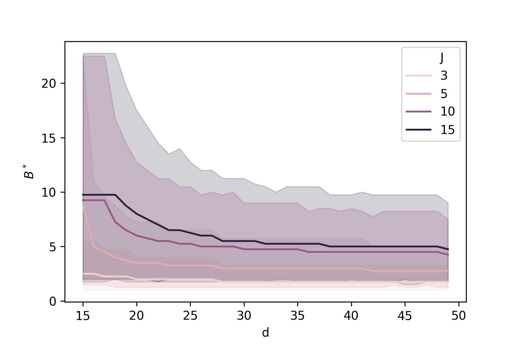
(a) $B^{*}$ by $J$ and $d$.

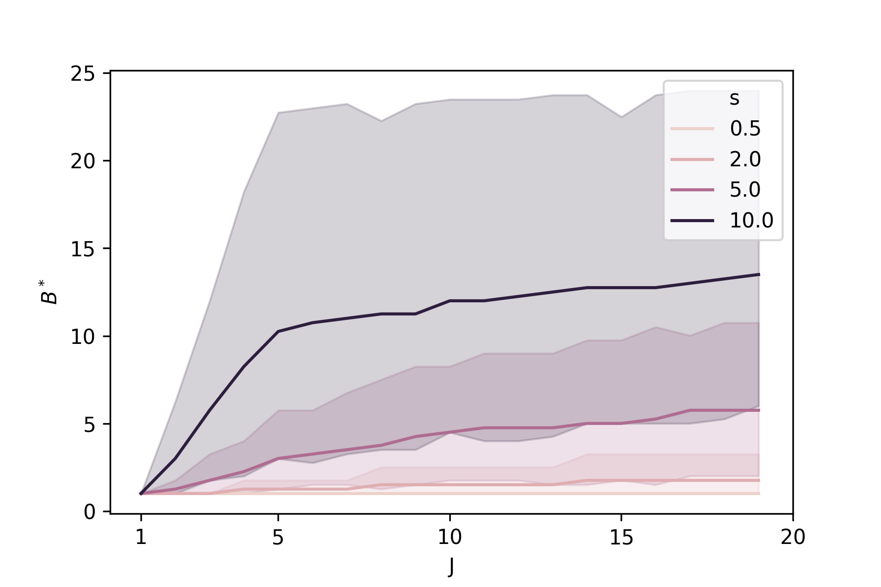
(b) $B^{*}$ by $s$ and $J$.

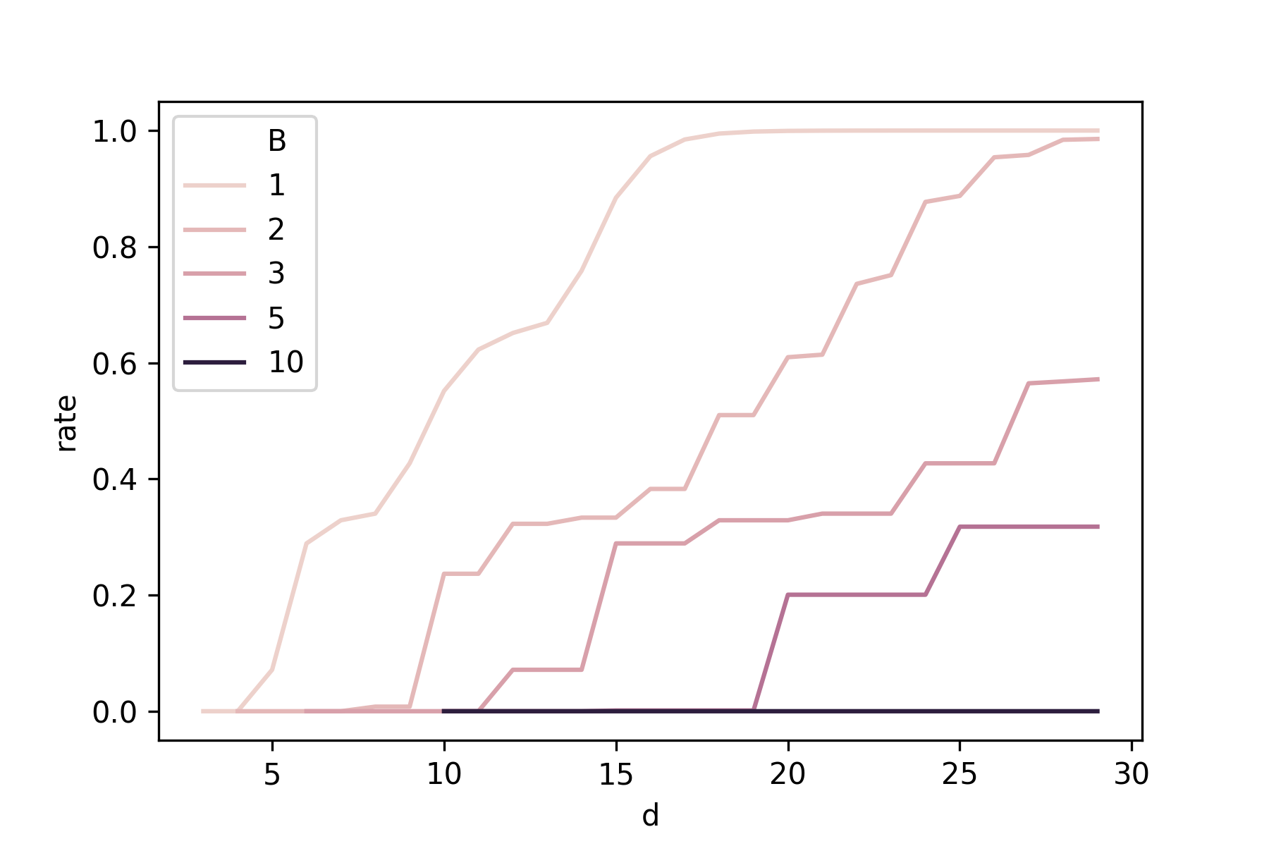
(c) Rate by $B$ and $d$.

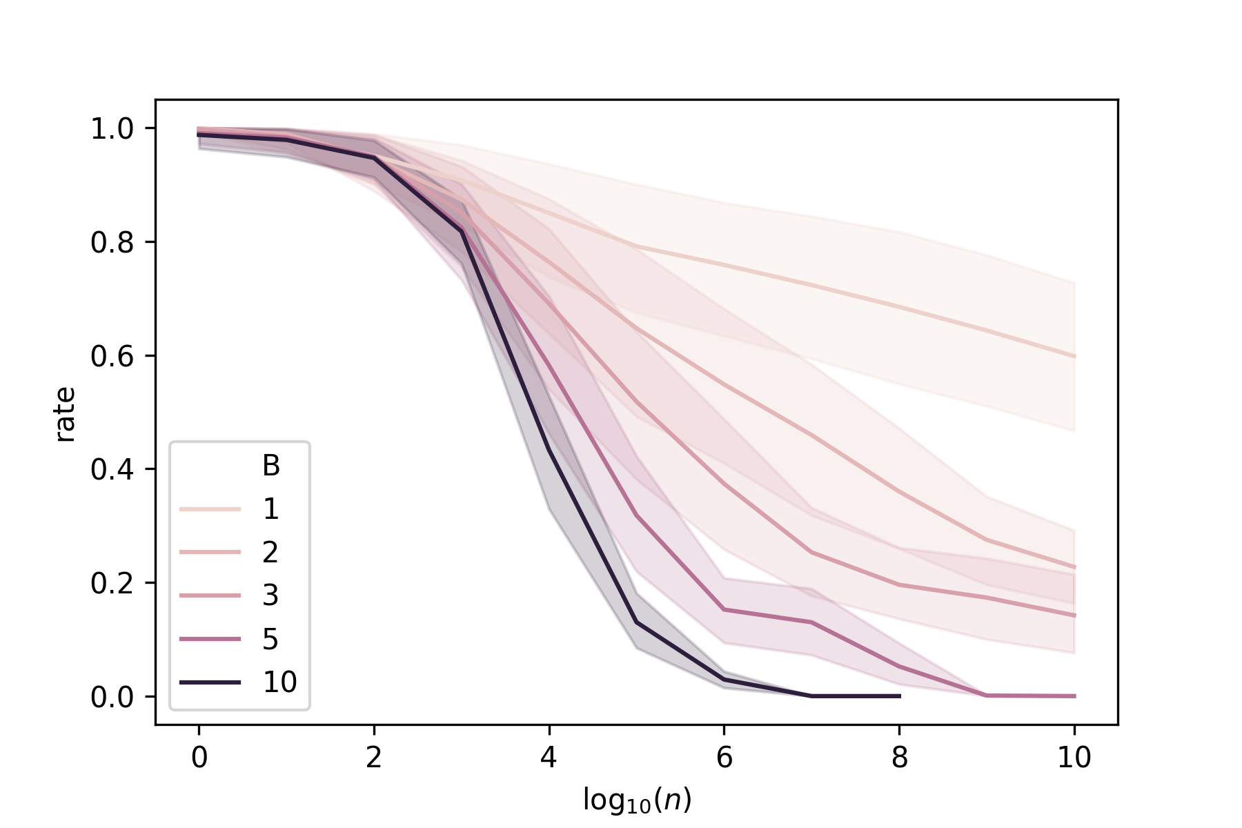
(d) Rate by $B$ and $n$.

Figure 1: Finite sample rates and the choice of partition number $B$.

• Notes: Panel (a) plots the upper bound on $B^{*}$ for different $J$ and $d$ values when $s=5$. Panel (b) shows the upper bound on $B^{*}$ for different $s$ and $J$ values when $d=40$. In both panels the solid lines and the bands are the means and confidence bands over values for $t\in[0.001,0.5]$. Panel (c) plots the finite sample rate, normalized to be bounded by 1, for different $B$ and $d$ values when $J=3$, $n=10^{7}$, $s=5$ and $t=0.05$. Panel (d) plots the same rate as panel (c) over different values of $n$, with confidence bands for values over $d\in[1,50]$. Discrete jumps in the curves are due to $d/B$ being coarsened to have integer values.

3 Bagged Polynomial Regression

Motivated by the theoretical insights we propose a bagged polynomial regression method. The aim of the method is to address the computational problem and slow rates when we have to estimate a large number of parameters while maintaining interpretability. We do so by relying on the feature splitting idea of partitioned series regression and through explicit regularization by penalization and model ensembling. This method draws from the drop-out idea for neural networks of only using some neurons in each training iteration [18] and from the model ensembling and bagging literature [4].

The BPR averages $M$ regression models trained on polynomial embeddings of degree $J$ of a random subset of basic features of size $F$. This setup allows us to choose $F$ and $k$ to control model complexity and make the problem computationally feasible even when we build polynomials of high degree. More precisely, we can write the output of the BPR model as

$$Y=\frac{1}{M}\sum_{m=1}^{M}\frac{1}{|N_{m}|}\sum_{i\in N_{m}}\langle W^{m},\Psi^{J}(X_{i}^{F_{m}})\rangle,$$ (18)

where $N_{m}$ is the sample of observations of size $|N_{m}|$ used to train model $m$, $W^{m}$ the weights for model $m$, and $\Psi^{J}$ is a function that generates polynomial features of degree $J$ from a random set of features denoted by $X_{i}^{F_{m}}$ of size $F$. The polynomial regression estimator for a model $m$ is defined by the $\hat{W}^{m}$ weights computed by solving the least squares problem for the restricted sample $N_{m}$ of observations and the polynomial features generated by $\Psi^{J}(X_{i}^{F_{m}})$. For simplicity, we assume that $S=|N_{m}|$ for all $m$, so that all models are trained on random samples of the same size. The following algorithm details the procedure:

Result: $\hat{Y}$.

Input: $Y\in\mathbb{R}^{n},X\in\mathbb{R}^{n\times d}$, $J$ degree of polynomial, $F$ number of features used, $M$ number of models trained, $S$ sample size used for training and $\lambda$ regularization parameter.

1

2for each $m\in\{1,\dots,M\}$ do

3       $X^{F_{m}}$ $\leftarrow$ random sample of $F$ features from $X$;

4       $N_{m}$ $\leftarrow$ random sample of $S$ observations indices;

5       generate polynomial features $\Psi^{J}(X_{i}^{F_{m}})$;

6       get $\hat{W}^{m}$ by minimizing

$$\sum_{i\in N_{m}}(Y_{i}-\langle W^{m},\Psi^{k}(X_{i}^{F_{m}})\rangle)^{2}+\lambda\|W^{m}\|_{2}^{2}$$

via stochastic gradient descent;

7       $\hat{Y}^{m}\leftarrow\frac{1}{S}\sum_{i\in N_{m}}Y_{i}-\langle\hat{W}^{m},\Psi^{J}(X_{i}^{F_{m}})\rangle$

8 end for

9$\hat{Y}\leftarrow\frac{1}{M}\sum_{m=1}^{M}\hat{Y}^{m}$;

Algorithm 1 Bagged Polynomial Regression

Note that we also include an $l_{2}$ regularization term denoted by $\lambda$, to avoid collinearity problems and improve out-of-sample fit, that can be hyper-tuned, along with the other parameters, using cross-validation.

Performance. By hyper-tuning the parameters $J$, $F$, $M$, $S$ and $\lambda$, BPR optimally chooses how to partition the feature space to build the polynomial features to navigate the approximation vs. estimation error trade-off. Choosing the hyper-parameters through cross-validation can be thought as estimating the optimal $B^{*}$ in Corollary 1.1 given the data setting. Furthermore, the additional $l_{2}$ penalty and model ensembling ensure that the generalization error is minimized.

This procedure can be used for both classification and regression problems. In the case of classification problems, we use logistic regression and minimize a logistic loss in step 5 of Algorithm 1, and instead of taking the average of the $M$ models we take the majority vote (median). In this case, bagging can be particularly useful as the activation function is non-linear so the models we train will have low bias and high variance. As in random forest, by taking the median/average of $M$ models we can successfully control the variance of the overall model and achieve a lower generalization error.

Interpretability. The BPR estimator is a good alternative to neural networks both in terms of performance and interpretability. Focusing on the case of classification, our estimator can be thought of as a weighted sum of logistic regression coefficients on our polynomial regressors. We weight all $M$ of our regressions equally – and if a regressor $X_{1}$ in included in a specific regression then the logistic coefficient $\beta_{1}$ will be weighted 1/$M$. Using logistic regression enables these $\beta_{1}$ parameters to have log-odds interpretations. Furthermore, using logistic regression makes sure we avoid the prediction problems of linear probability models that can predict values outside the support of our outcome model. These features make understanding how our variables impact the prediction of our outcome much more transparent than in the neural network case.

4 Application

In this section, we describe our computational results when the BPR is applied to the MNIST dataset [14]. We selected this dataset as it is a standard dataset for training and testing deep learning methods. Using MNIST enables us to compare our method to state-of-the-art prediction methods easily. We approach the prediction task as a classification problem with ten classes. The data has 60,000 observations and 784 features, where each feature is one pixel of the handwritten image and the labels are the 0-9 digits. Given the high-dimension of the feature space ($d=784$) standard polynomial regression may be ill-suited for this task, so we consider this example as a suitable setting to compare BPR to other models.

Main model. Our primary model for predicting the ten digits is based on combining ten different BPR models; one for each digit we are trying to predict, similarly to [8]. For each one of these ten models, we train a BPR model to predict whether the observed image is one of the digits or not. Each digit-specific model is trained following the BPR algorithm described in the last section. In practice, the number of bags we use is in the range 20 - 500. However, the main empirical results we report in this paper are for models that use a subset of features of size between 20 and 80 and polynomial embeddings of degree 2. When we create the polynomial embedding for a given subset of features, we include all of the base terms, all of the interactions between these terms, and their second-order polynomials. Note that this yields a number of transformed features smaller than the one used in the theoretical derivations, where all interactions were built. We choose not to include higher order interactions to reduce the computational burden of training the model.

Results. We start by showing how the choice of the number of bags and the number of features per sub-model affects performance for the a one digit prediction task. Figure 2 shows that models trained on only 40 out of the 784 features already achieve near perfect accuracy, while increasing the number of bags improves the convergence path. This can be seen in Figure 2 as larger ensemble models (dashed lines) only require 30 features per model to reach a near perfect accuracy. This empirical result highlights the theoretical intuition that it may be optimal to generate polynomial features only for subgroups to improve the convergence rate.

Our second empirical finding is that BPR can perform close to the state-of-the-art for the MNIST task while using significantly less parameters. Table 1 shows the out-of-sample accuracy for a BPR trained with 100 bags, 80 features per model and degree 2 polynomial transformations.

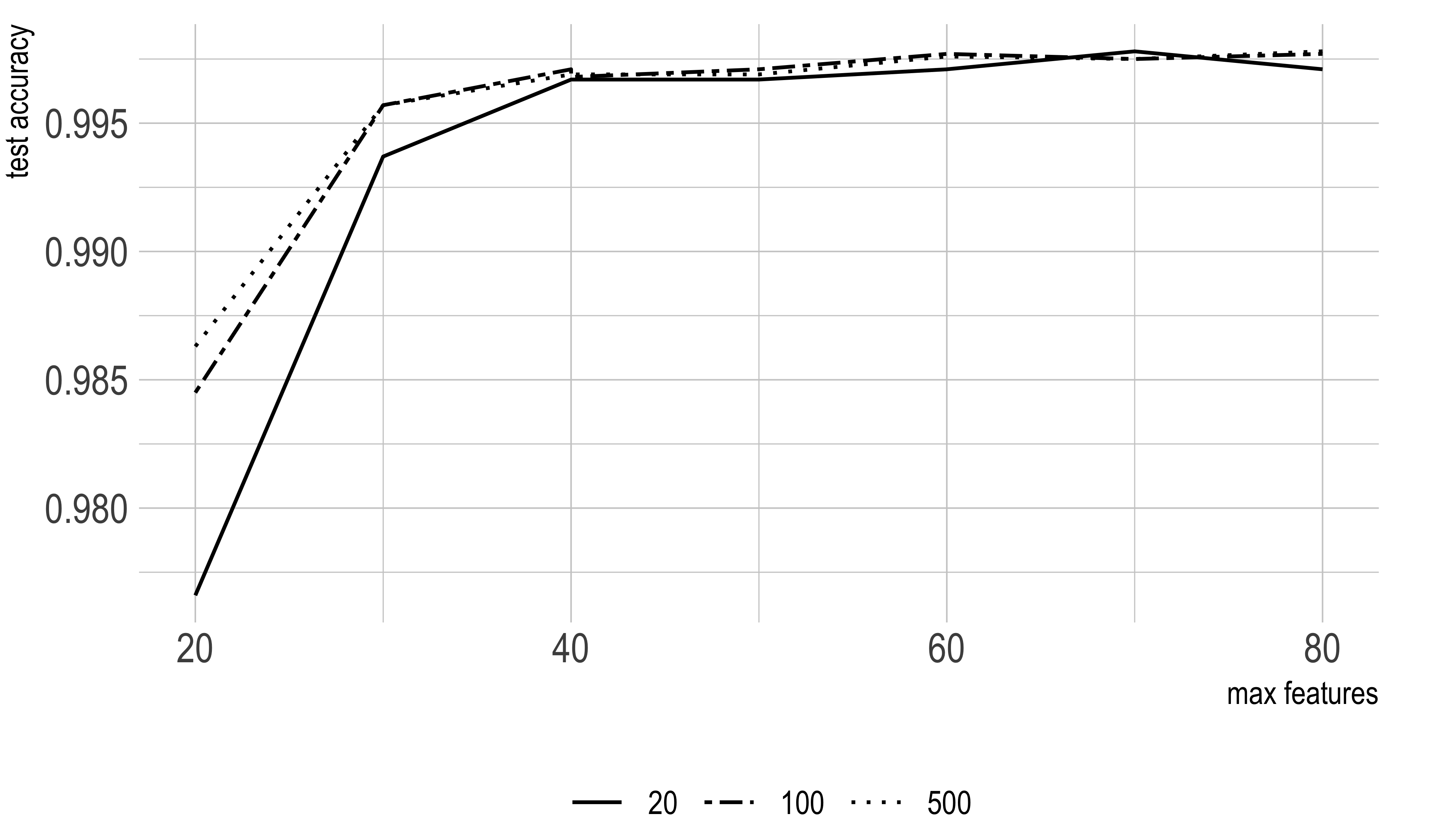
Figure 2: Test Accuracy By Number of Estimators.

• Notes: This figure shows test accuracy for predicting the digit 1 in the MNIST data. On the x-axis we have max features - the number of base regressors used in each weak estimator. On the y-axis we have the test accuracy which gives the percent of the digits correctly classified. The different dashed lines represent the number of models bagged in each case.

Table 1: MNIST 10 digit out-of-sample accuracy comparison between methods.

method	BPR	Polynomial regression	Convolutional Neural Net	State-of-the-Art
accuracy	97.58%	95.94%	99.03 %	99.79%

Comparison. In Table 1 we compare our BPR method to the polynomial regression method of [8], and the two neural net approaches cited in their paper. Our model achieves higher accuracy than [8], while estimating fewer parameters: [8] have 18,740 parameters per sub-model and our BPR is trained on 3,321 per sub-model. This is striking as we sample our features randomly for each sub-model, while [8] use the less naive approach of including the baseline interactions terms of features that are bordering pixels. More importantly, both our method and [8] use fewer parameters than the state-of-the-art and convolutional neural network that typically contain on the order of hundreds of thousands if not millions of parameters per model. Finally, it is important to note that we did not fully hyper-tune our BPR. We expect that a fully tuned BPR, with careful hyper-tuning of the parameters $J$, $F$, $M$, $S$ and $\lambda$, would be able to perform closer to the state-of-the-art.

5 Conclusion

In this paper, we highlight why polynomial regression, while offering more interpretability than neural networks and being able to approximate the same function classes, is rarely used in practice. By deriving new finite sample and asymptotic $L^{2}$ rates for series regression estimators, we show that the convergence rate for polynomial regression can be very slow. However, the rate can be improved when the polynomial embeddings are generated group-wise for partitions of the feature space rather than for all features. The improvement is particularly salient when the function class we are trying to estimate is smooth. Motivated by these results, we propose the use of BPR instead of standard polynomial regression as a potential substitute for neural networks. BPR draws from the theoretical insight of building polynomial embeddings for subsets of the feature space and from ensembling models by averaging multiple estimators to improve the out-of-sample performance. Finally, we show that it can perform similarly to more complex models, using fewer parameters, in an application to the MNIST handwritten digit data set.

Limitations and Future Work. This paper provides a formal reason why polynomial regression is ill-suited for prediction tasks in high-dimensional settings. However a limitation of the paper is that, while the main theorem (Theorem 1) applies to a large class of series regression models, the result for polynomial regression (Corollary 1.1) focuses on specific function classes (Holder smoothness of degree s) and a subset of models (partitioned polynomial regression). Future work should expand the application of the main result to include ensembles of polynomial regression models and formally link our theory with our proposed estimator the BPR. Furthermore, a more extensive benchmarking exercise should be carried out to compare BPR with existing state of the art methods. Given that in this paper we did not fully tune BPR, we expect future results to validate that BPR can perform as well as neural networks.

Societal and Ethic Impact. BPR could be used in a wide variety of applications, including recommender systems, modeling in economics, and classification problems more generally. Our method can be used to help researchers develop high performance classification models that retain interpretability. The interpretability of BPR over neural networks could help researchers better understand the underlying models and the importance of certain features in their data. While more accurate classification methods have the risk of helping to automate or disrupt various industries. For example, better recommender systems could lead to more market concentration by firms that gather large amounts of data, hurting consumer welfare. By proposing a method that is more interpretable and fully open source, we hope to improve competition and transparency.

Supplementary Materials

A.1 Holder class of smoothness order s

We replicate here the definition given in [2]. For $s>1$, we can define $\Sigma_{s}(\mathcal{X})$ as follows. For a tuple of $d$ non-negative integers $\alpha$, let

$$D^{\alpha}=\partial^{\alpha_{1}}_{x_{1}}\dots\partial_{x_{d}}^{\alpha_{d}}.$$ (A.1)

Let $\bar{s}$ denote the largest integer smaller than $s$, then $\Sigma_{s}(\mathcal{X})$ is defined as the set of all functions $f:\mathcal{X}\to\mathbb{R}$ such that $f$ is $\bar{s}$ times continuously differentiable and for some $C>0$,

$$|D^{\alpha}f(x)-D^{\alpha}f(\tilde{x})\leq C\left(\sum_{j}(x_{j}-\tilde{x}_{j})^{2}\right)^{(s-\bar{s})/2}$$ (A.2)

and $|D^{\beta}f(x)|\leq C$ for all $x,\tilde{x}\in\mathcal{X}$ and $\alpha,\beta$ nonnegative integer tuples such that $\sum_{j}\alpha_{j}=\bar{s}$ and $\sum_{j}\beta_{j}\leq\bar{s}$.

A.2 Rudelson and Vershynin 2007

A useful result to derive the finite sample rates in our setting is Theorem 3.1 in [17] which is a refinement of Rudelson’s LLN [16]:

Theorem A.1 (Rudelson and Vershynin 2007).

Let y be a random vector in $\mathbb{R}^{k}$ such that there exists an integer $M$ for which $\|y\|_{2}\leq M$ and under appropriate normalization $\|Ey\otimes y\|_{2}\leq 1$. For $y_{1},\dots,y_{n}$ independent copies of y, let

$$a\equiv C\sqrt{\frac{\log n}{n}}M.$$ (A.3)

Then, if $a<1$

$$E\left\|\frac{1}{n}\sum_{i}y_{i}\otimes y_{i}-Ey\otimes y\right\|_{2}\leq a,$$ (A.4)

and for $t\in(0,1)$

$$P\left(\left\|\frac{1}{n}\sum_{i}y_{i}\otimes y_{i}-Ey\otimes y\right\|_{2}>t\right)\leq 2e^{-ct^{2}/a^{2}},$$ (A.5)

for some positive constants $c$ and $C$, where $\|\cdot\|_{2}$ denotes the operator norm for matrices.

A.3 Proof of Theorem 1

Proof.

This proof adapts [2] by using [17] instead of [16] and deriving the asymptotic rates for non leading terms. Then the results are extended to include a finite sample rate under a subgaussianity assumption. Notation wise let $\|\cdot\|$ denote the Euclidean norm and $\|\cdot\|_{op}$ denote the operator norm for matrices. It will be useful to note that for a matrix $A$ and vector $b$, $\|Ab\|\leq\|A\|_{op}\|b\|$.

Start by observing that

$$\|\hat{g}-g\|_{F,2}\leq\|p^{\prime}\hat{\beta}-p^{\prime}\beta\|_{F,2}+c_{k}$$ (A.6)

and under normalization $Q=I$

$$\|p^{\prime}\hat{\beta}-p^{\prime}\beta\|_{F,2}=\|\hat{\beta}-\beta\|.$$ (A.7)

By the triangle inequality,

$$\|\hat{\beta}-\beta\|\leq\|\hat{Q}^{-1}\mathbb{E}_{n}[p_{i}\epsilon_{i}]\|+\|\hat{Q}^{-1}\mathbb{E}_{n}[p_{i}r_{i}]\|.$$ (A.8)

where $\hat{Q}=\frac{1}{n}\sum_{i}p_{i}\otimes p_{i}$. Applying [17] for $p_{i}$ we get that

$$E\|\hat{Q}-Q\|\leq a,$$ (A.9)

when $a\leq 1$ for $a=C\sqrt{\frac{\log n}{n}}\xi_{k}$ for a finite constant $C$. Furthermore, it can be shown that all eigenvalues of $\hat{Q}$ are bounded away from zero so the inverse exists and is well defined. This allows us to apply the continuous mapping theorem for the inverse. Next, we bound the two terms that depend on $\hat{Q}^{-1}$.

By Markov’s inequality, for $t>0$

$$P(\|\hat{Q}^{-1}\mathbb{E}_{n}[p_{i}\epsilon_{i}]\|>t) \leq\frac{E\|(\hat{Q}^{-1}-Q+Q)\mathbb{E}_{n}[p_{i}\epsilon_{i}]\|}{t}$$ (A.10)

$$\leq\frac{E\|(\hat{Q}^{-1}-Q)\mathbb{E}_{n}[p_{i}\epsilon_{i}]+Q\mathbb{E}_{n}[p_{i}\epsilon_{i}]\|}{t}$$ (A.11)

$$\leq\frac{E\|(\hat{Q}^{-1}-Q)\mathbb{E}_{n}[p_{i}\epsilon_{i}]\|+E\|\mathbb{E}_{n}[p_{i}\epsilon_{i}]\|}{t}$$ (A.12)

$$\lesssim\frac{(a+1)\sqrt{k/n}}{t}$$ (A.13)

where the $\sqrt{k/n}$ comes from

$$E\|\mathbb{E}_{n}[p_{i}\epsilon_{i}]\|^{2}=E[\sigma_{i}^{2}p_{i}^{\prime}p_{i}/n]\lesssim k/n,$$ (A.14)

given that $\sigma_{i}^{2}\leq\bar{\sigma}^{2}<\infty$ and the $a$ term comes from applying the Rudelson and Vershynin result and the continuous mapping theorem for the inverse.

We proceed similarly for the $\|\hat{Q}^{-1}\mathbb{E}_{n}[p_{i}r_{i}]\|$ term by observing that

$$\|\hat{Q}^{-1/2}\mathbb{E}_{n}[p_{i}r_{i}]\|\leq\mathbb{E}_{n}[r_{i}^{2}].$$ (A.15)

Then, by Markov’s inequality for $t>0$ when $c_{k}\to 0$

$$P(\|\hat{Q}^{-1}\mathbb{E}_{n}[p_{i}r_{i}]\|>t) \leq\frac{E\|(\hat{Q}^{-1}-Q)\mathbb{E}_{n}[p_{i}r_{i}]\|+E\|\mathbb{E}_{n}[p_{i}r_{i}]\|}{t}$$ (A.16)

$$\lesssim\frac{(a+1)c_{k}}{t}$$ (A.17)

where the $c_{k}$ term comes from $E[r_{i}^{2}]\leq c_{k}^{2}$ and we note that the all eigenvalues of $\hat{Q}^{1/2}$ are bounded away from zero with high probability.

Combining both bounds yields the desired asymptotic result.

For the finite sample rate, note that for some $\delta>0$,

$$P(\|\hat{\beta}-\beta\|>\delta) \leq P(\|\hat{Q}^{-1}\mathbb{E}_{n}[p_{i}\epsilon_{i}]\|+\|\hat{Q}^{-1}\mathbb{E}_{n}[p_{i}r_{i}]\|>\delta)$$ (A.18)

$$\leq P(\|(\hat{Q}^{-1}-Q+Q)\mathbb{E}_{n}[p_{i}\epsilon_{i}]\|>\delta/2)+P(\|(\hat{Q}^{-1}-Q+Q)\mathbb{E}_{n}[p_{i}r_{i}]\|>\delta/2)$$ (A.19)

$$\leq P(\|\hat{Q}^{-1}-Q\|_{op}\|\mathbb{E}_{n}[p_{i}\epsilon_{i}]\|>\delta/4)+P(\|\hat{Q}^{-1}-Q\|_{op}\|\mathbb{E}_{n}[p_{i}r_{i}]\|>\delta/4)$$ (A.20)

$$\quad+P(\|\mathbb{E}_{n}[p_{i}\epsilon_{i}]\|>\delta/4)+P(\|\mathbb{E}_{n}[p_{i}r_{i}]\|>\delta/4)$$ (A.21)

$$\leq 2P(\|\hat{Q}^{-1}-Q\|_{op}>\sqrt{\delta}/2)$$ (A.22)

$$\quad+P(\|\mathbb{E}_{n}[p_{i}\epsilon_{i}]\|>\sqrt{\delta}/2)+P(\|\mathbb{E}_{n}[p_{i}r_{i}]\|>\sqrt{\delta}/2)$$ (A.23)

$$\quad+P(\|\mathbb{E}_{n}[p_{i}\epsilon_{i}]\|>\delta/4)+P(\|\mathbb{E}_{n}[p_{i}r_{i}]\|>\delta/4),$$ (A.24)

where the last inequality follows from $P(\{w|x(w)y(w)>t\})\leq P(\{w|x(w)>\sqrt{t}\}\cap\{w|y(w)>\sqrt{t}\})\leq P(\{w|x(w)>\sqrt{t}\})+P(\{w|y(w)>\sqrt{t}\})$. The first term can be bounded directly by applying [17]:

$$P(\|\hat{Q}^{-1}-Q\|_{op}>\sqrt{\delta}/2)\lesssim 2\exp\left\{-c\frac{\delta}{4a^{2}}\right\},$$ (A.25)

where $a$ is defined as above. For the terms that depend on $\epsilon_{i}$ let $S_{n}=\|\mathbb{E}_{n}[p_{i}\epsilon_{i}]\|$ and observe that under the assumption that $\epsilon_{i}$ is subGaussian and that $p_{i}$ is uniformly bounded we have that $S_{n}-ES_{n}$ is a centered subGaussian random variable with coefficient $\nu_{i}=\xi_{k}\sigma_{i}$. Then, for $\delta>0$ by a suitable Hoeffding’s inequality

$$P(\|\mathbb{E}_{n}[p_{i}\epsilon_{i}]\|>\delta) =P(S_{n}-ES_{n}+ES_{n}>\delta)$$ (A.26)

$$\leq P(S_{n}-ES_{n}>\delta/2)+P(ES_{n}>\delta/2)$$ (A.27)

$$\leq\exp\left\{-\frac{n\delta^{2}}{4\xi_{k}\bar{\sigma}}\right\},$$ (A.28)

where the second step requires that $ES_{n}\leq\sqrt{k/n}<\delta/2$ and $\bar{\sigma}$ could be included in the constant term. For the terms that depends on $r_{i}$ observe that $R_{n}=\|\mathbb{E}[p_{i}r_{i}]\|$ is a uniformly bounded random variable given our assumptions on $p$ and $r$. Therefore, we can show that $R_{n}-ER_{n}$ is a subGaussian random variable with variance factor $4nc_{k}\xi_{k}$. In Belloni et al. 2015 it is shown that $ER_{n}\lesssim\frac{c_{k}\xi_{k}}{\sqrt{n}}$. Hence, applying Hoeffding’s inequality again

$$P(\|\mathbb{E}_{n}[p_{i}r_{i}]\|>\delta) =P(R_{n}-ER_{n}+ER_{n}>\delta)$$ (A.29)

$$\leq P(R_{n}-ER_{n}>\delta/2)+P(ER_{n}>\delta/2)$$ (A.30)

$$\lesssim\exp\left\{-\frac{n\delta^{2}}{8\xi_{k}c_{k}}\right\},$$ (A.31)

where the second step requires that $\frac{c_{k}\xi_{k}}{\sqrt{n}}<\delta/2$. Grouping all constants and noting that for $\delta<1$, $\sqrt{\delta}>\delta$, we can derive the finite sample bound by three exponential terms. It can be stated as follows, for $t\in(0,1)$, $c_{k}\leq t/2$, and $\frac{c_{k}\xi_{k}}{\sqrt{n}},\sqrt{k/n}<t/8$,

$$P(\|\hat{g}-g\|_{F,2}>\delta) \leq P(\|p^{\prime}\hat{\beta}-p^{\prime}\beta\|_{F,2}+c_{k}>\delta)$$ (A.32)

$$\leq P(\|p^{\prime}\hat{\beta}-p^{\prime}\beta\|_{F,2}>\delta/2)$$ (A.33)

$$\lesssim\exp\left\{-\frac{t}{a^{2}}\right\}+\exp\left\{-\frac{nt^{2}}{\xi_{k}c_{k}}\right\}+\exp\left\{-\frac{nt^{2}}{\xi_{k}}\right\}.$$ (A.34)

∎

A.4 Proof of Corollary 1.1

Proof.

Under the appropriate normalization it is shown in [15] that $\xi_{k}\lesssim k$ and in [2] that $c_{k}\lesssim k^{-s/d}$ for the holder class of smoothness $s$ denoted by $\Sigma_{s}(\mathcal{X})$. Observe that the approximation bound is decreasing in $k$ as $s,d>0$, so when $k\asymp B(J)^{d/B}$ it follows that $c_{k}\lesssim B^{-s/d}(J)^{\lfloor-s/B\rfloor}$. Similarly, $\xi_{k}\lesssim B(J)^{\lfloor d/B\lfloor}\leq B(J)^{d/B}$.

Next, consider the conditions of Theorem 2 $c_{k}\leq t/2$ and $\frac{c_{k}\xi_{k}}{\sqrt{n}}\lor\sqrt{k/n}<t/8$. Given $c_{k}\leq t/2$, a sufficient inequality for the second condition to hold is $\xi_{k}<\sqrt{n}/4$. Hence, under the bound $\xi_{k}\lesssim k$ a sufficient condition to apply Theorem 2 given $c_{k}\leq t/2$ is $n>16k^{2}$ (large enough $n$). To complete the prove then, it remains to show that the finite sample bound in Theorem 2 achieves a unique minimum with respect to $B$ given the other parameters.

Consider the function $G$ as defined in the Corollary statement, given that $e^{x}$ is a strictly increasing convex function, it follows that $G$ is non-increasing in $B$ for any $n,d,J,s>0$ and $t>0$ such that $d\geq s$. Furthermore, the image of $G$ is contained in $[0,3]$ and $B$ belongs to a compact set in $\mathbb{Z}^{+}$ given by $\mathcal{B}(n,d,J,s,t,)=\{B\in\mathbb{R}|B^{-s/d}(J/B)^{-s}\leq t/2\}\cap\mathbb{Z}^{+}$. Therefore, for any $n,d,J$, $s$ and $t$ such that $d\geq s$, there exists a unique $B\in\mathcal{B}(n,d,J,s)$ that minimizes $G$ which coincides with $\sup\mathcal{B}(n,d,J,s)$. Rewriting the condition $d^{-s/d}(J)^{-s/B}\leq t/2$ we get that the desired result. This implies that $G$ is a well defined function with respect to $B$. ∎

References

- [1] Donald WK Andrews and Yoon-Jae Whang “Additive interactive regression models: circumvention of the curse of dimensionality” In Econometric Theory 6.4 Cambridge University Press, 1990, pp. 466–479
- [2] Alexandre Belloni, Victor Chernozhukov, Denis Chetverikov and Kengo Kato “Some new asymptotic theory for least squares series: Pointwise and uniform results” In Journal of Econometrics 186.2, 2015, pp. 345–366
- [3] Leo Breiman “Bagging predictors” In Machine learning 24.2 Springer, 1996, pp. 123–140
- [4] Leo Breiman “Random forests” In Machine learning 45.1 Springer, 2001, pp. 5–32
- [5] Matias D Cattaneo and Max H Farrell “Optimal convergence rates, Bahadur representation, and asymptotic normality of partitioning estimators” In Journal of Econometrics 174.2 Elsevier, 2013, pp. 127–143
- [6] Xi Cheng, Bohdan Khomtchouk, Norman Matloff and Pete Mohanty “Polynomial regression as an alternative to neural nets” In arXiv preprint arXiv:1806.06850, 2018
- [7] George Cybenko “Approximation by superpositions of a sigmoidal function” In Mathematics of control, signals and systems 2.4 Springer, 1989, pp. 303–314
- [8] Matt Emschwiller, David Gamarnik, Eren C Kızıldağ and Ilias Zadik “Neural networks and polynomial regression. demystifying the overparametrization phenomena” In arXiv preprint arXiv:2003.10523, 2020
- [9] Max H Farrell, Tengyuan Liang and Sanjog Misra “Deep neural networks for estimation and inference” In Econometrica 89.1 Wiley Online Library, 2021, pp. 181–213
- [10] Kurt Hornik “Approximation capabilities of multilayer feedforward networks” In Neural networks 4.2 Elsevier, 1991, pp. 251–257
- [11] Khashayar Khosravi, Greg Lewis and Vasilis Syrgkanis “Non-parametric inference adaptive to intrinsic dimension” In arXiv preprint arXiv:1901.03719, 2019
- [12] Mark A Kramer “Nonlinear principal component analysis using autoassociative neural networks” In AIChE journal 37.2 Wiley Online Library, 1991, pp. 233–243
- [13] Alex Krizhevsky, Ilya Sutskever and Geoffrey E Hinton “Imagenet classification with deep convolutional neural networks” In Advances in neural information processing systems 25, 2012
- [14] Yann LeCun “The MNIST database of handwritten digits” In http://yann. lecun. com/exdb/mnist/, 1998
- [15] Whitney K Newey “Convergence rates and asymptotic normality for series estimators” In Journal of econometrics 79.1 Elsevier, 1997, pp. 147–168
- [16] Mark Rudelson “Random vectors in the isotropic position” In Journal of Functional Analysis 164.1 Elsevier, 1999, pp. 60–72
- [17] Mark Rudelson and Roman Vershynin “Sampling from large matrices: An approach through geometric functional analysis” In Journal of the ACM (JACM) 54.4 ACM New York, NY, USA, 2007, pp. 21–es
- [18] Nitish Srivastava et al. “Dropout: a simple way to prevent neural networks from overfitting” In The journal of machine learning research 15.1 JMLR. org, 2014, pp. 1929–1958
- [19] Charles J Stone “Optimal global rates of convergence for nonparametric regression” In The annals of statistics JSTOR, 1982, pp. 1040–1053
- [20] Dmitry Yarotsky “Error bounds for approximations with deep ReLU networks” In Neural Networks 94 Elsevier, 2017, pp. 103–114