A Panorama of Viable $F(R)$ Gravity Dark Energy Models

Abstract

In this work we shall study the late-time dynamics of several $F(R)$ gravity models. By appropriately expressing the field equations in terms of the redshift and of a statefinder function, we shall solve numerically the field equations using appropriate physical motivated initial conditions. We consider models which, by construction, are described by a nearly $R^{2}$-model at early epochs and we fine tune the parameters to achieve viability and compatibility with the latest Planck constraints at late times. Such models provide a unified description of inflation and dark energy era and notably a common feature of all the models is the presence of dark energy oscillations. Furthermore, we show that, in contrast to general relativistic fluids and scalar field descriptions, a large spectrum of different dark energy physics is generated by simple $F(R)$ gravity models, varying from phantom, to nearly de Sitter and to quintessential dark energy eras.

I Introduction

Unambiguously, the observation that the Universe is currently accelerating is one of the most unexpected and fascinating feature of the current cosmological evolution. Dark energy is a mystery in modern theoretical cosmology, and several theoretical proposals can in principle describe successfully this cosmological era. In the context of simple general relativity, the dark energy era can be described by quintessence fields, and also by the rather unmotivated and unappealing interacting fluids approach. However, the scalar field description fails to describe the dark energy era in a self-consistent way, if the dark energy era is phantom, which is a probability according to the current Planck cosmological constraints on cosmological parameters Planck:2018vyg . Modified gravity in its various forms reviews1 ; reviews2 ; reviews3 ; reviews4 ; reviews5 can successfully describe the dark energy era in a self-consistent way, without resorting to phantom scalar fields, in order to have an equation of state (EoS) parameter slightly tuned to the phantom. The most prominent and simpler among modified gravities is $F(R)$ gravity Nojiri:2003ft ; Capozziello:2005ku ; Capozziello:2004vh ; Capozziello:2018ddp ; Hwang:2001pu ; Cognola:2005de ; Nojiri:2006gh ; Song:2006ej ; Capozziello:2008qc ; Bean:2006up ; Capozziello:2012ie ; Faulkner:2006ub ; Olmo:2006eh ; Sawicki:2007tf ; Faraoni:2007yn ; Carloni:2007yv ; Nojiri:2007as ; Capozziello:2007ms ; Deruelle:2007pt ; Appleby:2008tv ; Dunsby:2010wg ; Odintsov:2020nwm ; Odintsov:2019mlf ; Odintsov:2019evb ; Oikonomou:2020oex ; Oikonomou:2020qah , in the context of which various cosmological eras can successfully be realized. More importantly, in the context of $F(R)$ gravity inflation and the dark energy era can be described in a unified way, see the pioneer work Nojiri:2003ft , and also Nojiri:2006gh ; Nojiri:2007as ; Appleby:2008tv ; Odintsov:2019evb ; Oikonomou:2020oex ; Oikonomou:2020qah for some recent developments. At first time the unification of the inflation with dark energy epoch in $F(R)$ gravity was proposed in Nojiri:2003ft . After that, several realistic models of $F(R)$ gravity unifying inflation with dark energy, and consistent with observational bounds were developed in Cognola:2007zu ; Nojiri:2007cq . In this line of research, in this work we shall present several dark energy $F(R)$ gravity models, which primordially are described by the $R^{2}$ model Starobinsky:1980te ; Bezrukov:2007ep and at late-times all these models mimic the $\Lambda$-Cold-Dark-Matter model ($\Lambda$CDM). All the models we shall present realize a viable dark energy era, with dark energy EoS parameter and dark energy density parameter compatible with the latest Planck constraints on cosmological parameters. With this work we aim to present a panorama of viable $f(R)$ gravity dark energy models which can also generate a viable inflationary era.

This paper is organized as follows: In section II we overview the formulation of $F(R)$ gravity which is suitable for describing the late-time dynamics of $F(R)$ gravity. We shall express the field equations in terms of the redshift as a dynamical parameter and we shall use a suitable statefinder parameter, capable of containing all the information needed for late-time dynamics. In section III we present several viable $F(R)$ gravity models which can produce a successful late-time era, in addition to a successful inflationary era. Finally, the conclusions follow at the end of the article.

II $F(R)$ Gravity Late-time Evolution Framework

Consider an $F(R)$ gravity model in the presence of perfect matter fluids, with action,

$$\centering\mathcal{S}=\int{d^{4}x\sqrt{-g}\left(\frac{F(R)}{2\kappa^{2}}+\mathcal{L}_{m}\right)}\,,\@add@centering$$ (1)

where $g$ denotes the determinant of the metric tensor $g^{\mu\nu}$ and $\mathcal{L}_{m}$ stands for the Lagrangian of the perfect matter fluids that are considered present. The term $F(R)$ describes an arbitrary function of the Ricci scalar $R$ and in our case it will be taking the form of,

$$F(R)=R+f(R).$$ (2)

We also note that $\kappa^{2}=8\pi G=\frac{1}{M_{p}^{2}}$, where $G$ is Newton’s constant and $M_{p}$ is the reduced Planck mass. For the background metric, we select the flat Friedmann-Robertson-Walker (FRW) metric with the following line element,

$$\centering ds^{2}=-dt^{2}+a(t)\sum_{i=1}^{3}dx_{i}^{2},\@add@centering$$ (3)

where $\alpha(t)$ is the scale factor. Given that the Ricci scalar for the FRW metric is equal to,

$$R=6\dot{H}+12H^{2},$$ (4)

by varying the action (1) with respect to the metric, we obtain the gravitational equations of motion,

$$3F_{R}H^{2}=\kappa^{2}\rho_{m}+\frac{F_{R}R-F}{2}-3H\dot{F}_{R}\,,$$ (5)

$$-2F_{R}\dot{H}=\kappa^{2}(\rho_{m}+R_{m})+\ddot{F}-H\dot{F}\,,$$ (6)

where $F_{R}=\frac{\partial F}{\partial R}$ and the “dot” denotes derivative with respect to cosmic time. $H=\frac{\dot{\alpha}}{\alpha}$ is the Hubble parameter and $\rho_{m},P_{m}$ stand for the matter fluids energy density and the corresponding pressure respectively. We can actually rewrite the field equations (5),(6) in the Einstein-Hilbert form for a flat FRW metric and we get,

$$3H^{2}=\kappa^{2}\rho_{tot}\ ,$$ (7)

$$-2\dot{H}=\kappa^{2}(\rho_{tot}+P_{tot})\ ,$$ (8)

where $\rho_{tot}$ is the total energy density of the effective cosmological fluid and $P_{tot}$ the corresponding pressure of it. We assume that the cosmological fluid has 3 main contributions, those of cold dark matter ($\rho_{m}$), of radiation ($\rho_{r}$) and of dark energy ($\rho_{DE}$) . Therefore we have, $\rho_{tot}=\rho_{m}+\rho_{r}+\rho_{DE}$ and $P_{tot}=P_{m}+P_{r}+P_{DE}$. The late-time evolution is predominantly driven by the dark energy fluid, the characteristics of which can be read off the Friedmann and Raychaudhuri equations, (5) and (6),

$$\rho_{DE}=\frac{F_{R}R-F}{2}+3H^{2}(1-F_{R})-3H\dot{F}_{R}\,,$$ (9)

$$P_{DE}=\ddot{F}-H\dot{F}+2\dot{H}(F_{R}-1)-\rho_{DE}\,.$$ (10)

However, instead of the cosmic time we prefer using the redshift as a dynamical variable to quantify evolution, which is defined as,

$$1+z=\frac{1}{a},$$ (11)

where we assumed that the present time scale factor is equal to unity, therefore $z=0$ at present. Furthermore, we introduce the statefinder function $y_{H}(z)$ Hu:2007nk ; Bamba:2012qi ; Odintsov:2020vjb ; Odintsov:2020nwm ; Odintsov:2020qyw ; reviews1 ,

$$y_{H}(z)=\frac{\rho_{DE}}{\rho_{m}^{(0)}}=\frac{H^{2}}{m_{s}^{2}}-(1+z)^{3}-\chi(1+z)^{4},$$ (12)

with $\rho_{m}^{(0)}$ denoting the energy density of the cold dark matter at present time, $m_{s}^{2}=\frac{\kappa^{2}\rho_{m}^{(0)}}{3}=H_{0}^{2}\Omega_{m}=1.37\times 10^{-67}eV^{2}$ is the mass scale and $\chi$ is defined as $\chi=\frac{\rho_{r}^{(0)}}{\rho_{m}^{(0)}}\simeq 3.1\times 10^{-4}$, where $\rho_{r}^{(0)}$ is the present time radiation energy density.

By combining the equations (7) , (2) and (12), we can express the Friedmann equation in terms of the statefinder $y_{H}$ and it reads,

$$\frac{d^{2}y_{H}}{dz^{2}}+J_{1}\frac{dy_{H}}{dz}+J_{2}y_{H}+J_{3}=0\,,$$ (13)

where the dimensionless functions $J_{1}$ , $J_{2}$ , $J_{3}$ are defined as follows,

$$J_{1}=\frac{1}{(z+1)}\Big{(}-3-\frac{1}{y_{H}+(z+1)^{3}+\chi(z+1)^{4}}\frac{1-F_{R}}{6m_{s}^{2}F_{RR}}\Big{)}\,,$$ (14)

$$J_{2}=\frac{1}{(z+1)^{2}}\Big{(}\frac{1}{y_{H}+(z+1)^{3}+\chi(z+1)^{4}}\frac{2-F_{R}}{3m_{s}^{2}F_{RR}}\Big{)}\,,$$ (15)

$$J_{3}=-3(z+1)-\frac{(1-F_{R})((z+1)^{3}+2\chi(z+1)^{4})+(R-F)/(3m_{s}^{2})}{(z+1)^{2}(y_{H}+(z+1)^{3}+\chi(z+1)^{4})}\frac{1}{6m_{s}^{2}F_{RR}}\,,$$ (16)

and $F_{RR}=\frac{\partial^{2}F}{\partial R^{2}}$. Also, the Ricci scalar as a function of the Hubble rate and of the redshift is equal to,

$$R=12H^{2}-6HH_{z}(1+z)\,,$$ (17)

so the Ricci scalar is an implicit function of the statefinder parameter $y_{H}$ and can be expressed in terms of it as follows,

$$R(z)=3\,m_{s}^{2}\left(-(z+1)\,\frac{dy_{H}(z)}{dz}+4y_{H}(z)+(1+z)^{3}\right)\,.$$ (18)

In order to study the late-time evolution of the universe using an $F(R)$ gravity approach, we need to solve (13) numerically for the redshift interval $z=[0,10]$ which demands determining the initial conditions. Note that the derivatives of the statefinder quantity $y_{H}(z)$ in terms of the redshift also appear in the dimensionless parameters $J_{i}$, see Eq. (18). Thus our aim is to solve numerically the differential equation (13), subject to physically motivated initial conditions. We consider the following physically motivated choice of initial conditions at $z_{f}=10$ Bamba:2012qi ; Odintsov:2020vjb ; Odintsov:2020nwm ; Odintsov:2020qyw ; reviews1 ,

$$y_{H}(z_{f})=\frac{\Lambda}{3m_{s}^{2}}\Big{(}1+\frac{1+z_{f}}{1000}\Big{)}\ ,\ \frac{dy_{H}(z)}{dz}\Big{|}_{z=z_{f}}=\frac{1}{1000}\frac{\Lambda}{3m_{s}^{2}},$$ (19)

where $\Lambda\simeq 11.895\times 10^{-67}eV^{2}$. The numerical analysis will yield the statefinder quantity $y_{H}(z)$ as a function of the redshift. From the obtained numerical solution $y_{H}(z)$, one can evaluate all the relevant physical quantities, such as the Hubble rate, the Ricci scalar, the energy density parameter $\Omega_{DE}(z)$, the dark energy EoS parameter, the total EoS parameter and the deceleration parameter. Specifically, the Hubble rate in terms of $y_{H}(z)$ is,

$$H(z)=m_{s}\sqrt{y_{H}(z)+(1+z)^{3}+\chi(1+z)^{4}}\,.$$ (20)

where $\chi$ is defined below Eq. (12). Also the Ricci scalar describing the curvature reads,

$$R(z)=3m_{s}^{2}\Big{(}4y_{H}(z)-(z+1)\frac{dy_{H}(z)}{dz}+(z+1)^{3}\Big{)},$$ (21)

and the energy density parameter $\Omega_{DE}(z)$ is given by,

$$\Omega_{DE}(z)=\frac{y_{H}(z)}{y_{H}(z)+(z+1)^{3}+\chi(z+1)^{4}}.$$ (22)

The dark energy EoS parameter is,

$$\omega_{DE}(z)=-1+\frac{1}{3}(z+1)\frac{1}{y_{H}(z)}\frac{dy_{H}(z)}{dz},$$ (23)

while the total EoS parameter reads,

$$\omega_{tot}(z)=\frac{2(z+1)H^{\prime}(z)}{3H(z)}-1\ ,$$ (24)

and finally the deceleration parameter is,

$$q(z)=-1-\frac{\dot{H}}{H^{2}}=-1-(z+1)\frac{H^{\prime}(z)}{H(z)},$$ (25)

where the “prime” denotes derivative with respect to the redshift. We also note that the Hubble rate is given by Eq. (20), while for the $\Lambda CDM$ model equals to

$$H_{\Lambda}(z)=H_{0}\sqrt{\Omega_{\Lambda}+\Omega_{M}(z+1)^{3}+\Omega_{r}(z+1)^{4}},$$ (26)

where $\Omega_{\Lambda}\simeq 0.68136$ and $\Omega_{M}\simeq 0.3153$. Also $H_{0}\simeq 1.37187\times 10^{-33}$eV is the present time Hubble rate according to the latest Planck data Planck:2018vyg .

Let us briefly discuss at this point the choice of the initial conditions (19) and the motivation for choosing these conditions. For a deeper analysis on this issue see also Bamba:2012qi . Basically the initial conditions (19) correspond to the behavior of the statefinder function $y_{H}(z)$ at large redshifts, so deeply in the matter domination era, multibillion years in our Universe’s past, well before the deceleration to acceleration transition point. Basically the redshift for which the initial conditions (19) should be valid is possibly well before $z\sim 2$. In such a case, $y_{H}(z)\ll(1+z)^{3}$ so one may solve the differential equation (13) around the auxiliary redshift $z_{0}$, which is a redshift well after the deceleration to acceleration transition corresponding to the late-time era. Deeply in the matter domination era, the scalar curvature is approximately $R\sim 3m_{s}^{2}(1+z)^{3}$. So by considering the differential equation (13) around $z\sim z_{0}+(z-z_{0})$ with $|z-z_{0}|\ll z$, and keeping leading order terms, the differential equation (13) becomes,

$$\frac{d^{2}y_{H}}{dz^{2}}+\frac{\alpha_{1}}{z-z_{0}}\frac{dy_{H}}{dz}+\frac{\beta_{1}}{(z-z_{0})^{2}}y_{H}=\zeta_{0}+\zeta_{1}(z-z_{0})\,,$$ (27)

where $\zeta_{0}$ and $\zeta_{1}$ are constants, and also $\alpha_{1}$ and $\beta_{1}$ are,

$$\alpha_{1}=-\frac{7}{2}-\frac{(1-F_{R}(R_{0}))F_{RRR}(R_{0})}{2F_{RR}(R_{0})^{2}},\,\,\,\beta_{1}=2+\frac{1}{R_{0}F_{RR}(R_{0})}+2\frac{(1-F_{R}(R_{0}))F_{RRR}(R_{0})}{F_{RR}(R_{0})^{2}}\,,$$ (28)

where $R_{0}$ is the curvature scalar at the redshift $z_{0}$. So by solving the differential equation (27) one obtains at leading order (we omit exponential decaying terms),

$$y_{H}(z)\simeq\alpha_{1}+\beta_{1}(z-z_{0})\,.$$ (29)

Hence at a redshift $z_{f}$ deeply in the matter domination era, one has a linear dependence of the statefinder function $y_{H}(z)$ in terms of the redshift. So this basically motivates the initial conditions of Eq. (19), for which we also allowed a physically motivated fine-tuning regarding the parameters $\alpha_{1}$ and $\beta_{1}$. It is notable though that the overall qualitative behavior of the models we shall present does not change, however if the initial conditions are changed, the values of the free parameters of the models that render each model viable, change, as is expected.

Also it is vital that every dark energy model which we shall discuss in the next section, satisfies the viability criteria that every $F(R)$ gravity must satisfy. These are reviews1 ; Zhao:2008bn ,

$$F^{\prime}(R)>0\,,\,\,\,F^{\prime\prime}(R)>0\,,$$ (30)

for $R>R_{0}$, with $R_{0}$ being the curvature at present day. So for each model these criteria should be satisfied, for all the curvatures from the present day up to the inflationary era, where $R\sim 12H_{I}^{2}$, with $H_{I}$ being the inflationary scale, which is assumed to be of the order $H_{I}\sim 10^{13}$GeV.

III Late-time $F(R)$ Gravity dynamics

In this section we present the results of the numerical analysis mentioned in the previous section for seven $F(R)$ gravity models. In essence, we calculate the present time values and plot the evolution of some of the aforementioned statefinder and physical quantities in the redshift interval $z=[0,10]$ and compare them with the $\Lambda CDM$ Model or the latest Planck data on cosmological parameters Planck:2018vyg . Another remark to be made is that we added a $R^{2}/M^{2}$ term in every function, where $M=3.04375\times 10^{22}$eV. The value for the parameter $M$, its actual value is determined by inflationary phenomenological reasons, and it is equal to $M=1.5\times 10^{-5}\left(\frac{N}{50}\right)^{-1}M_{p}$ Appleby:2009uf , where $N$ being the $e$-foldings number during the inflationary era. So for $N\sim\mathcal{O}(50-60)$ one gets the value $M=3.04375\times 10^{22}$eV. The $R^{2}$ term has a key role in the unification of the early-time and the late-time eras, since it is the dominant term in the evolution of the early universe, where $R\sim H_{I}^{2}$ where $H_{I}$ is the inflationary scale., but becomes insignificant compared to the other terms at late times where $R$ becomes comparable to the cosmological constant. On the contrary when $R\sim H_{I}^{2}$ where $H_{I}$ is the inflationary scale, the $R^{2}$ term dominates over the dark energy terms an thus the inflationary era is controlled by the $R^{2}$ model.

III.1 Type I $\Lambda$CDM-like with logarithmic $F(R)$ Gravity: Model 1

We shall begin with the following $F(R)$ function,

$$F(R)=R+\frac{R^{2}}{M^{2}}+\frac{b}{1+\log{(R/R_{0})}},$$ (31)

where $\log$ denotes the base 10 logarithm and $b$ and $R_{0}$ are free parameters with dimensions of $eV^{2}$ (dimensions of $[m]^{2}$ in natural units). We choose the values $b=0.5m_{s}^{2}$ and $R_{0}=220m_{s}^{2}$ and using Eqs. (13)-(26) we find that for $z=0$, that is the present time, the values of the dark energy density parameter and EoS parameter are $\Omega_{DE}(0)=0.6834$ and $\omega_{DE}(0)=-1.0372$, which fall into the viability limits of the Planck constraints, $\Omega_{DE}=0.6847\pm 0.0073$ and $\omega_{DE}=-1.018\pm 0.031$. In Fig.1 we plot $\omega_{DE}$ for the redshift interval $z=[0,10]$ and we observe that the oscillations amplify as the redshift increases. Unfortunately, oscillations are a characteristic of the behavior of the statefinders in most $F(R)$ gravity theories in the redshift interval $z=[5,10]$, and this a well known feature that has also been pointed out in the literature, see Hu:2007nk ; Bamba:2012qi ; Elizalde:2011ds ; Nadkarni-Ghosh:2021mws . In Fig. 1 we also plot the deceleration parameter, with $q(0)=-0.5632$ and the function $y_{H}$. Furthermore, in Fig. 2 we plot the total (effective) EoS parameter, which has a present time value of $\omega_{tot}(0)=-0.7088$. This $F(R)$ Gravity model provides a viable late-time phenomenology which is proved by the values of the parameters that either comply with the latest constraints or are very close to the observed ones, as one can see in Table. 1.

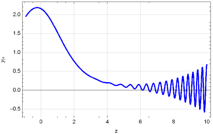
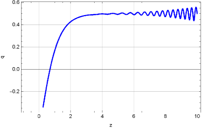
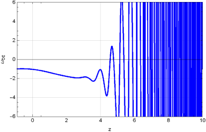
Figure 1: Plots of the statefinder quantities $y_{H}(z)$ (upper left plot), the deceleration parameter $q(z)$ (upper right plot) and the dark energy EoS parameter $\omega_{DE}(z)$ (lower plot) as functions of the redshift for the logarithmic type $F(R)$ model of Eq. (31) for $b=0.5m_{s}^{2}$ and $R_{0}=220m_{s}^{2}$.

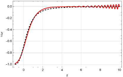
Figure 2: Plot of total (effective) EoS parameter for the logarithmic type $F(R)$ model of Eq. (31) for $b=0.5m_{s}^{2}$ and $R_{0}=220m_{s}^{2}$ (red line) and for the $\Lambda$CDM model (dashed line) as functions of the redshift.

One indication that this model can give good results is given by the plots of Fig. 1. The deceleration parameter varies from $q(0)\simeq-0.5$ to $q(10)\simeq 0.5$, illustrating the passage from a decelerating era to an accelerated one. Furthermore, the total EoS parameter is almost equal to the dark energy EoS parameter, both being driven to $\simeq 1$ and $\omega_{tot}(10)\simeq 0$, indicating that a (decelerating) matter dominated era is followed by a (accelerating) dark energy dominated era. The Hubble parameter is found equal to $H=1.36918\times 10^{-33}$eV, a value very close to the observed one today based on the CMB measurements.

III.2 Type I $\Lambda$CDM-like with logarithmic format $F(R)$: Model 2

Moving on, we examine another logarithmic type $F(R)$ function,

$$F(R)=R+\frac{R^{2}}{M^{2}}-\frac{b}{c+1/\log(R/R_{0})},$$ (32)

where, as before, $b$ and $R_{0}$ are free parameters with dimensions of $eV^{2}$ (dimensions of $[m]^{2}$ in natural units) and $c$ is a dimensionless free parameter. After some investigation we concluded that by setting the free parameters’ values equal to $b=11.81\Lambda,c=1.5,R_{0}=m_{s}^{2}/100$ we get a viable phenomenology. Specifically, the present time values for the dark energy density parameter, the dark energy EoS parameter and the total EoS parameter are $\Omega_{DE}(0)=0.6876$, $\omega_{DE}(0)=-0.9891$ and $\omega_{tot}=-0.6801$ respectively. The values of the first two parameters comply with the Planck constraints and the latter is very close to the value calculated for the $\Lambda$CDM model, that is $\omega_{\Lambda tot}=-0.6847$. The similarity between the evolution of the total EoS parameter between the two models is obvious in Fig. 4.

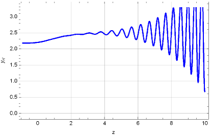
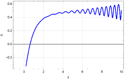
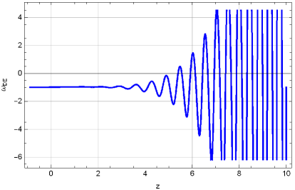
Figure 3: Plots of the statefinder quantities $y_{H}(z)$ (upper left plot), the deceleration parameter $q(z)$ (upper right plot) and the dark energy EoS parameter $\omega_{DE}(z)$ (lower plot) as functions of the redshift for the logarithmic type $F(R)$ model of Eq. (32) for $b=11.81\Lambda,c=1.5,R_{0}=m_{s}^{2}/100$.

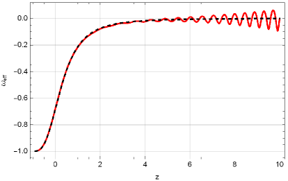
Figure 4: Plot of total (effective) EoS parameter for the logarithmic type $F(R)$ model of Eq. (32) for $b=11.81\Lambda,c=1.5,R_{0}=m_{s}^{2}/100$ (red line) and for the $\Lambda$CDM model (dashed line) as functions of the redshift.

In Fig. 3 we also plot the functions $y_{H}(z)$ and $q(z)$, with the latter taking the value $q(0)=-0.5201$, close to the one from the $\Lambda$CDM too. Finally, we shall mention that the calculated Hubble rate is $H=1.3785\times 10^{-33}$eV. The qualitative remarks from the plots are similar to the ones mentioned for the previous case.

III.3 Type I $\Lambda$CDM-like with exponential format $F(R)$ Model

Let us proceed to the results obtained from the study of the following $F(R)$ model,

$$F(R)=R+\frac{R^{2}}{M^{2}}-\frac{b}{c+\exp(-R/R_{0})},$$ (33)

where, as per usual, $b$ and $R_{0}$ are free parameters with dimensions of $eV^{2}$ (dimensions of $[m]^{2}$ in natural units) and $c$ is a dimensionless free parameter. We followed the numerical solution path described in the previous section and by setting $b=20\Lambda,c=2$ and $R_{0}=m_{s}^{2}/0.00091$ we concluded to a viable dark energy for $F(R)$ Gravity model. The plot of $y_{H}(z)$ is given in Fig. 5 and using this solution of (13) along with Eq. (20)-(24) we can construct the rest of the plots of Fig. 5 and Fig. 6 and calculate the present day values of the cosmological quantities of interest. The dark energy energy density parameter and EoS parameter at $z=0$ are evaluated to be $\Omega_{DE}=0.6918$ and $\omega_{DE}=-0.9974$, while the total EoS parameter is found equal to $\omega_{tot}=-0.6899$. Moreover, the deceleration parameter at present time is estimated equal to $q(0)=-0.5349$ and the Hubble rate equal to $H=1.3878\times 10^{-33}$eV. The values of the cosmological parameters $\Omega_{DE}$ and $\omega_{DE}$ comply with the latest Planck constraints and, generally, the values of all the aforementioned parameters belong within the observational regime.

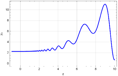
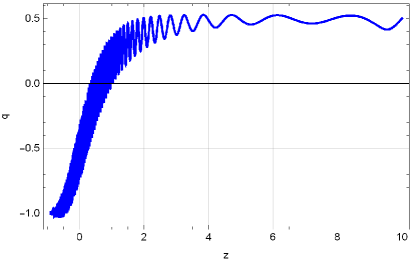
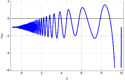
Figure 5: Plots of the statefinder quantities $y_{H}(z)$ (upper left plot), the deceleration parameter $q(z)$ (upper right plot) and the dark energy EoS parameter $\omega_{DE}(z)$ (lower plot) as functions of the redshift for the logarithmic type $F(R)$ model of Eq. (33) for $b=20\Lambda,c=2$ and $R_{0}=m_{s}^{2}/0.00091$.

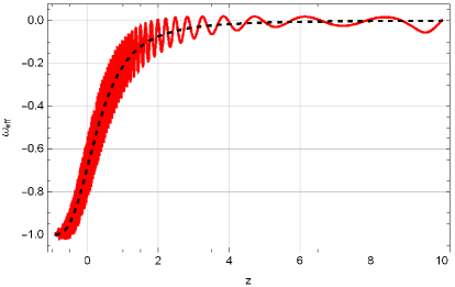
Figure 6: Plot of total (effective) EoS parameter for the logarithmic type $F(R)$ model of Eq. (33) for $b=20\Lambda,c=2$ and $R_{0}=m_{s}^{2}/0.00091$ (red line) and for the $\Lambda$CDM model (dashed line) as functions of the redshift.

One characteristic of this model is that the oscillations accompanying the evolution of these cosmological parameters are evident in the whole $z=[0,10]$ redshift range, losing amplitude but rising in frequency as we move from $z=10$ to $z=0$. It is widely suggested that the oscillations in $F(R)$ gravity theories are a model-dependent characteristic, therefore we attribute this to the exponential nature of the model.

III.4 Type I $\Lambda$CDM-like with polynomial format $F(R)$ Model

Another $F(R)$ model with interesting results comes from the following function,

$$F(R)=R+\frac{R^{2}}{M^{2}}-\alpha\frac{b(R/R_{0})^{n}}{c(R/R_{0})^{n}+d},$$ (34)

where $b,c,d,n$ are dimensionless parameters and $\alpha,R_{0}$ are free parameters with dimensions of $eV^{2}$ (dimensions of $[m]^{2}$ in natural units). We set $\alpha=1.4\Lambda$, $b=1$, $c=0.2$ , $d=0.04$, $R_{0}=m_{s}^{2}$ and $n=0.3$ and following the numerical analysis described in the previous section we find the present time values of the statefinder quantities of interest. In Fig. 7 we plot the quantities $y_{H}$ , $q$, $\omega_{DE}$ and in Fig. 8 the total EoS parameter $\omega_{tot}$ as functions of the redshift for the interval $z=[0,10]$. Specifically for the present day values, this model gives $\Omega_{DE}(0)=0.6851$, $\omega_{DE}(0)=-0.9887$, $q(0)=-0.5160$, $\omega_{tot}=-0.6773$ and $H=1.37295\times 10^{-33}$eV. It is obvious that for the chosen initial conditions and values for the free parameters, the values of the cosmological quantities for these model belong within the desired range.

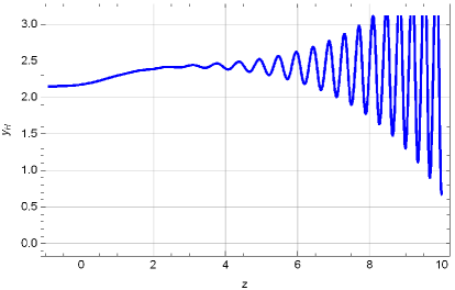
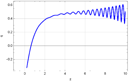
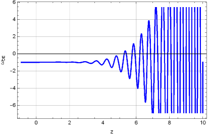
Figure 7: Plots of the statefinder quantities $y_{H}(z)$ (upper left plot), the deceleration parameter $q(z)$ (upper right plot) and the dark energy EoS parameter $\omega_{DE}(z)$ (lower plot) as functions of the redshift for the logarithmic type $F(R)$ model of Eq. (34) for $\alpha=1.4\Lambda$, $b=1$, $c=0.2$ , $d=0.04$, $R_{0}=m_{s}^{2}$ and $n=0.3$.

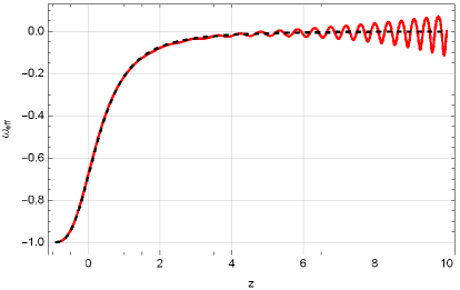
Figure 8: Plot of total (effective) EoS parameter for the logarithmic type $F(R)$ model of Eq. (34) for $\alpha=1.4\Lambda$, $b=1$, $c=0.2$ , $d=0.04$, $R_{0}=m_{s}^{2}$ and $n=0.3$ (red line) and for the $\Lambda$CDM model (dashed line) as functions of the redshift.

III.5 Type II $\Lambda$CDM-like with logarithmic format $F(R)$ model

Next we shall consider another type of $F(R)$ gravity function,

$$F(R)=R+\frac{R^{2}}{M^{2}}-\alpha R_{0}\log(1+R/R_{0}),$$ (35)

where $\alpha$ is a dimensionless free parameter and $R_{0}$ is another free parameter with dimensions of $eV^{2}$ (dimensions of $[m]^{2}$ in natural units). This type of $F(R)$ gravities were introduced and studied in Nojiri:2003ni ; Bamba:2014mua . The results from the study of this model for $R_{0}=m_{s}^{2}\times 10^{-64}$ and $\alpha=10^{63}\Lambda/m_{s}^{2}=2.0045\times 10^{63}$ are presented in Fig. 9, Fig. 10 and Table 1. In particular, for this $F(R)$ model we find that $\Omega_{DE}(0)=0.68596$, which is compatible with the Planck constraint $\Omega_{DE}=0.6847\pm 0.0073$ and $\omega_{DE}(0)=-0.9962$, which also is compatible with the Planck constraint $\omega_{DE}=-1.018\pm 0.031$. Additionally, we evaluate the present time values of to total EoS parameter $\omega_{tot}(0)=-0.6832$ , the deceleration parameter $q(0)=-0.5249$ and the Hubble rate $H=1.37483\times 10^{-33}$eV. Thus, we have another model with viable dark energy phenomenology for the values for the free parameters mentioned above and the initial conditions (19).

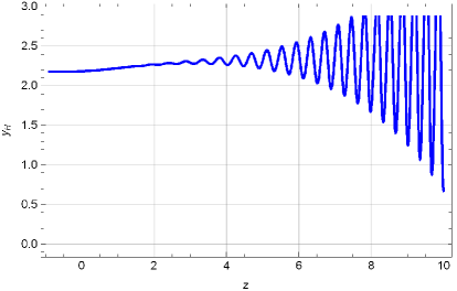
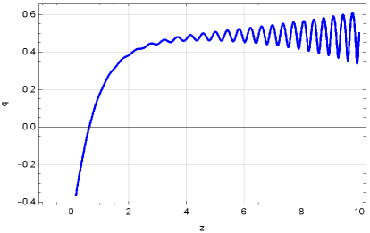
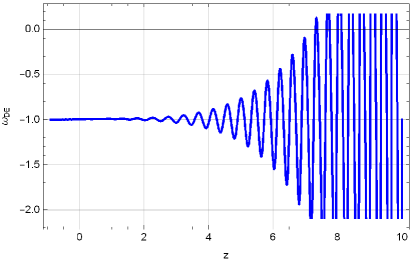
Figure 9: Plots of the statefinder quantities $y_{H}(z)$ (upper left plot), the deceleration parameter $q(z)$ (upper right plot) and the dark energy EoS parameter $\omega_{DE}(z)$ (lower plot) as functions of the redshift for the logarithmic type $F(R)$ model of Eq. (35) for $R_{0}=m_{s}^{2}\times 10^{-64}$ and $\alpha=10^{63}\Lambda/m_{s}^{2}=2.0045\times 10^{63}$.

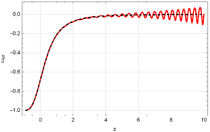
Figure 10: Plot of total (effective) EoS parameter for the logarithmic type $F(R)$ model of Eq. (35) for $R_{0}=m_{s}^{2}\times 10^{-64}$ and $\alpha=10^{63}\Lambda/m_{s}^{2}=2.0045\times 10^{63}$ (red line) and for the $\Lambda$CDM model (dashed line) as functions of the redshift.

III.6 Type II $\Lambda$CDM-like with exponential format $F(R)$ model

We shall proceed our examination with yet another exponential type $F(R)$ function,

$$F(R)=R+\frac{R^{2}}{M^{2}}-b[c-\exp(-R/R_{0})],$$ (36)

where $b,R_{0}$ are free parameters with dimensions of $eV^{2}$ (dimensions of $[m]^{2}$ in natural units) and $c$ is a dimensionless free parameter. For these parameters we pick the values $c=7.5$, $b=\Lambda$ and $R_{0}=m_{s}^{2}/0.0005$ and the viability of this model is evident from the results shown in Fig. 11, Fig. 12 and Table 1. In detail, for the dark energy density parameter we obtain $\Omega_{DE}(0)=0.6847$ and for the dark energy EoS parameter $\omega_{DE}(0)=-1.0367$, values that belong within the range of the Planck constraints. As for the rest cosmological parameters we find that $q(0)=-0.5647$, $\omega_{tot}=-0.7098$ and $H=1.37212\times 10^{-33}$eV. At this point we shall discuss the qualitative characteristics of the plots in Fig. 11 and 12. It is obvious from Eqs. (20)-(24) that the evolution of the cosmological parameters depends on the one of the statefinder quantity $y_{H}$ and as can be seen in Fig. 11 , $y_{H}$ is plagued with oscillations, as usual, with their amplitude falling and their frequency rising significantly as we move forward from the redshift $z=10$ to $z=0$, with that characteristic being passed to the other parameters as well. This observation was made before for another exponential-type $F(R)$ model, indicating that the nature of the models is indeed the cause.

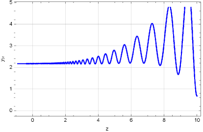
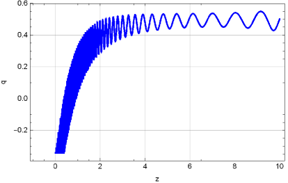
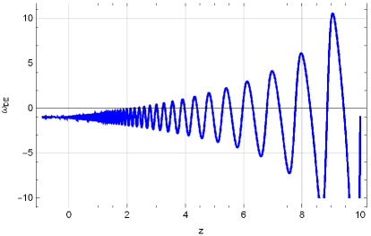
Figure 11: Plots of the statefinder quantities $y_{H}(z)$ (upper left plot), the deceleration parameter $q(z)$ (upper right plot) and the dark energy EoS parameter $\omega_{DE}(z)$ (lower plot) as functions of the redshift for the logarithmic type $F(R)$ model of Eq. (36) for $c=7.5$, $b=\Lambda$ and $R_{0}=m_{s}^{2}/0.0005$.

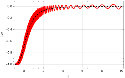
Figure 12: Plot of total (effective) EoS parameter for the logarithmic type $F(R)$ model of Eq. (36) for $c=7.5$, $b=\Lambda$ and $R_{0}=m_{s}^{2}/0.0005$ (red line) and for the $\Lambda$CDM model (dashed line) as functions of the redshift.

III.7 Type III $\Lambda$CDM-like with polynomial format $F(R)$ model

The last $F(R)$ function we shall study is,

$$F(R)=R+\frac{R^{2}}{M^{2}}-b\frac{c-(R_{0}/R)^{n}}{d+(R_{0}/R)^{n}},$$ (37)

where $c,d,n$ are dimensionless free parameters and $b,R_{0}$ are free parameters with dimensions of $eV^{2}$ (dimensions of $[m]^{2}$ in natural units). For this model, by setting $b=\Lambda$ , $R_{0}=m_{s}^{2}$, $c=27$ , $d=3$ and $n=0.01$ we find that $\Omega_{DE}(0)=0.6867$ and $\omega_{DE}(0)=-0.9976$, which satisfy the latest Planck mission constraints. Moreover, the numerical analysis gives $\omega_{tot}=-0.6849$, $q(0)=-0.5274$ and $H=1.37626\times 10^{-33}$eV, values very close to the observed ones at present time. These results are also shown in Table 1, compared to the ones of the other models along and the $\Lambda$CDM model or Planck constraints if provided. In Fig. 13 and Fig. 14 we plot the evolution of some of the cosmological quantities for the redshift interval $z=[0,10]$.

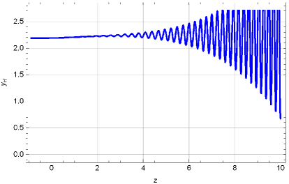
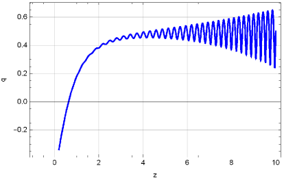
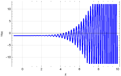
Figure 13: Plots of the statefinder quantities $y_{H}(z)$ (upper left plot), the deceleration parameter $q(z)$ (upper right plot) and the dark energy EoS parameter $\omega_{DE}(z)$ (lower plot) as functions of the redshift for the logarithmic type $F(R)$ model of Eq. (37) for $b=\Lambda$ , $R_{0}=m_{s}^{2}$ , $c=27$, $d=3$ and $n=0.01$.

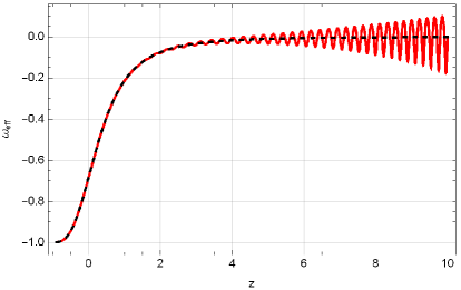
Figure 14: Plot of total (effective) EoS parameter for the logarithmic type $F(R)$ model of Eq. (37) for $b=\Lambda$ , $R_{0}=m_{s}^{2}$ , $c=27$, $d=3$ and $n=0.01$ (red line) and for the $\Lambda$CDM model (dashed line) as functions of the redshift.

Table 1: Cosmological Parameters Values at present day for the $F(R)$ Gravity models studied in this work, quoting only their corresponding Equation in the text, the $\Lambda$CDM Model and the Planck 2018 data where available (quoting only the Planck 2018 constraint if available). The values for the $\Lambda$CDM model are obtained by using the Hubble rate in Eq. (26) and Eqs. (22), (23), (24) and (25).

Parameter	(31)	(32)	(33)	(34)	(35)	(36)	(37)	Planck 2018 or SNe I$A^{a}$	$\Lambda$CDM
$\Omega_{DE}(0)$	$0.6834$	$0.6876$	$0.6918$	$0.6851$	$0.68596$	$0.6847$	$0.6867$	$0.6847\pm 0.0073$	-
$\omega_{DE}(0)$	$-1.0372$	$-0.9891$	$-0.9974$	$-0.9887$	$-0.9962$	$-1.0367$	$-0.9976$	$-1.018\pm 0.031$	-
$q(0)$	$-0.5632$	$-0.5201$	$-0.5349$	$-0.5160$	$-0.5249$	$-0.5647$	$-0.5274$	$-0.38\pm 0.05$ (SNe I$A^{a}$)	$-0.535$
$\omega_{tot}(0)$	$-0.7088$	$-0.6801$	$-0.6899$	$-0.6773$	$-0.6832$	$-0.7098$	$-0.6849$	-	$-0.68467$
$H\times 10^{-33}$eV	$1.36918$	$1.3785$	$1.3878$	$1.37295$	$1.37483$	$1.37212$	$1.37626$	$1.37187$	$1.37187$

At this point, let us investigate if the viability criteria (30) are satisfied for all the models studied in the this and the previous subsections. In Fig. 15 we plot the behavior of the derivatives $F^{\prime}(R)$ (upper left plot) and $F^{\prime\prime}(R)$ (upper right and bottom plots) in terms of the redshift in the range $z=[0,10]$. The Model 1 of Eq. (31) corresponds to the blue curve, the Model 2 of Eq. (32) corresponds to the pink curve, the type I $\Lambda$CDM-like with exponential format $F(R)$ model of Eq. (33) corresponds to the yellow curve, the type I $\Lambda$CDM-like with polynomial format $F(R)$ model of Eq. (34) corresponds to the green curve, the type II $\Lambda$CDM-like with logarithmic format $F(R)$ model of Eq. (35) corresponds to the red curve, the type III $\Lambda$CDM-like with polynomial format $F(R)$ model of Eq. (36) corresponds to the black dashed curve, and finally the type II $\Lambda$CDM-like with exponential format $F(R)$ model of Eq. (37) corresponds to the purple dashed curve. In the upper left plot of Fig. 15, where the $F^{\prime}(R)$ is plotted as a function of the redshift, it can be seen that the all the models satisfy the viability criterion and also that the models are identical similar regarding the values of $F^{\prime}(R)$. In fact, as it can be seen from the upper left plot, all the models are indistinguishable. In the upper right plot of Fig. 15 we present the values of $F^{\prime\prime}(R)$ as a function of the redshift for the models of Eqs. (32), (33), (34), (35), (36) and (37), and it can be seen that the viability criteria are satisfied and also some of the models are indistinguishable. The model of Eq. (31) is compared to the other models regarding the value of $F^{\prime\prime}(R)$ in the bottom plot of Fig. 15, since it is quite different from the other models, but regardless it also satisfies the viability criteria.

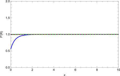
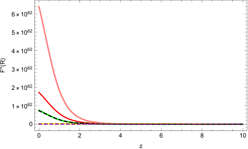
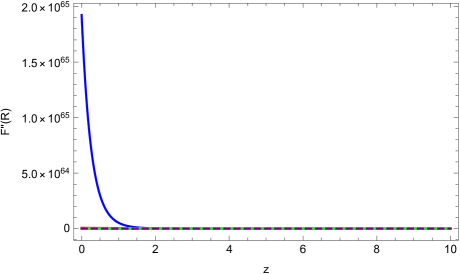
Figure 15: The terms $F^{\prime}(R)$ (upper left plot) and $F^{\prime\prime}(R)$ (upper right and bottom plot) as functions of the redshift in the redshift range $z=[0,10]$, for the models of Eqs. (31) (blue curve), (32) (pink curve), (33) (yellow curve), (34) (green curve), (35) (red curve), (36) (black curve) and (37) (purple curve). The viability criteria are satisfied for all the models.

The viability are also satisfied for higher redshifts, let us see this explicitly by considering inflationary scales of the curvature, when $H\sim H_{I}$, then $R\sim 12H_{I}^{2}$. For all the models we have $F^{\prime\prime}(R)\sim 2.1588\times 10^{-45}$eV^-1, and $F^{\prime}(R)\sim 3.59056$, hence the viability conditions (30) are satisfied too for inflationary scales. Also it is important to note that the reason for which the values of $F^{\prime}(R)$ and $F^{\prime\prime}(R)$ are the same for all the models is that the $F(R)$ gravity at early times is dominated by the $R^{2}$ term, and it can be checked that if we calculate $F^{\prime}(R)$ and $F^{\prime\prime}(R)$ by only keeping the $R^{2}$ term, we end up to the same values for $F^{\prime}(R)$ and $F^{\prime\prime}(R)$ we quoted above. This result was expected, since the models were engineered in such a way so that at early times the $R^{2}$ term dominates.

As an overall comment let us note that in principle there is a large range of values of the free parameters of the models we studied, for which the viability is guaranteed. However, the free parameters depend strongly on the values of the rest of free variables, so certain amount of fine-tuning is required so that the viability of each model is obtained.

It is also notable to mention that the starting redshift $z_{f}$ used in the initial conditions (19) also affects the viability of the models. We checked all the models by using different values for the starting redshift and a general conclusion is that as the initial redshift changes, the values of the free parameters must be changed for each model in order to achieve the viability of the models. This also mentioned in the relevant literature Nadkarni-Ghosh:2021mws . However we omit the details for different starting redshifts for brevity, since the overall qualitative picture is the same.

Finally, let us note that all the different seven models we considered, have more or less the same late-time qualitative behavior, since all of them mimic the $\Lambda$CDM model and predict viable dark energy related physical parameters. The differences is that some models predict a phantom evolution (Models (25) and (30)) while others predict a quintessential accelerating era (Models (26)-(29) and (31)).

IV Conclusions

In this paper we investigated several models of $F(R)$ gravity which may generated a viable dark energy era at late times and an $R^{2}$-like inflationary era primordially. We considered several different functional forms for the $F(R)$ gravities, varying from logarithmic models to exponential and power-law models. We expressed the field equations as functions of the redshift and we quantified our analysis by introducing a statefinder function $y_{H}(z)$ which basically measures the deformation from the Einstein-Hilbert gravity caused by the $F(R)$ gravity terms. By appropriately choosing the initial conditions at the last stages of the matter domination era for the statefinder function $y_{H}(z)$ and its derivative with respect to the redshift, we solved numerically the field equations and we derived the behavior of several physical quantities and statefinders. Specifically we were interested in the total EoS parameter, the dark energy EoS parameter, the dark energy density parameter and the deceleration parameter, which is the most characteristic statefinder available. As we demonstrated, a large spectrum of distinct late time cosmologies can be realized by different $F(R)$ gravity models. Specifically, it is possible to realize phantom, nearly de-Sitter and quintessential dark energy eras with simple $F(R)$ gravity models, without resorting to phantom scalar fields or relativistic fluids of any sort. With this work we aimed to provide a panorama of viable $F(R)$ gravity models which can describe inflation and dark energy in an unified manner, and we also aimed to demonstrate the large spectrum of different physics generated by simple $F(R)$ gravity models. It is a challenge to test some of these models regarding their primordial gravitational waves predictions, the reason being the behavior during the radiation domination era. In a future work we aim to present the predictions for the primordial gravitational waves spectrum of some of these models but also to consider ways to reduce the dark energy oscillations, which are present in all the models.

References

- (1) N. Aghanim et al. [Planck], Astron. Astrophys. 641 (2020), A6 [erratum: Astron. Astrophys. 652 (2021), C4] doi:10.1051/0004-6361/201833910 [arXiv:1807.06209 [astro-ph.CO]].
- (2) S. Nojiri, S. D. Odintsov and V. K. Oikonomou, Phys. Rept. 692 (2017) 1 [arXiv:1705.11098 [gr-qc]].
-
(3)
S. Capozziello, M. De Laurentis,
Phys. Rept. 509, 167 (2011);
V. Faraoni and S. Capozziello, Fundam. Theor. Phys. 170 (2010). - (4) S. Nojiri, S.D. Odintsov, eConf C0602061, 06 (2006) [Int. J. Geom. Meth. Mod. Phys. 4, 115 (2007)].
- (5) S. Nojiri, S.D. Odintsov, Phys. Rept. 505, 59 (2011);
- (6) A. de la Cruz-Dombriz and D. Saez-Gomez, Entropy 14 (2012) 1717 [arXiv:1207.2663 [gr-qc]].
- (7) S. Nojiri and S. D. Odintsov, Phys. Rev. D 68 (2003), 123512 doi:10.1103/PhysRevD.68.123512 [arXiv:hep-th/0307288 [hep-th]].
- (8) S. Capozziello, V. F. Cardone and A. Troisi, Phys. Rev. D 71 (2005), 043503 doi:10.1103/PhysRevD.71.043503 [arXiv:astro-ph/0501426 [astro-ph]].
- (9) S. Capozziello, C. A. Mantica and L. G. Molinari, Int. J. Geom. Meth. Mod. Phys. 16 (2018) no.01, 1950008 doi:10.1142/S0219887819500087 [arXiv:1810.03204 [gr-qc]].
- (10) S. Capozziello, V. F. Cardone and M. Francaviglia, Gen. Rel. Grav. 38 (2006), 711-734 doi:10.1007/s10714-006-0261-x [arXiv:astro-ph/0410135 [astro-ph]].
- (11) J. c. Hwang and H. Noh, Phys. Lett. B 506 (2001), 13-19 doi:10.1016/S0370-2693(01)00404-X [arXiv:astro-ph/0102423 [astro-ph]].
- (12) G. Cognola, E. Elizalde, S. Nojiri, S. D. Odintsov and S. Zerbini, JCAP 02 (2005), 010 doi:10.1088/1475-7516/2005/02/010 [arXiv:hep-th/0501096 [hep-th]].
- (13) S. Nojiri and S. D. Odintsov, Phys. Rev. D 74 (2006), 086005 doi:10.1103/PhysRevD.74.086005 [arXiv:hep-th/0608008 [hep-th]].
- (14) Y. S. Song, W. Hu and I. Sawicki, Phys. Rev. D 75 (2007), 044004 doi:10.1103/PhysRevD.75.044004 [arXiv:astro-ph/0610532 [astro-ph]].
- (15) S. Capozziello, V. F. Cardone and V. Salzano, Phys. Rev. D 78 (2008), 063504 doi:10.1103/PhysRevD.78.063504 [arXiv:0802.1583 [astro-ph]].
- (16) R. Bean, D. Bernat, L. Pogosian, A. Silvestri and M. Trodden, Phys. Rev. D 75 (2007), 064020 doi:10.1103/PhysRevD.75.064020 [arXiv:astro-ph/0611321 [astro-ph]].
- (17) S. Capozziello and M. De Laurentis, Annalen Phys. 524 (2012), 545-578 doi:10.1002/andp.201200109
- (18) T. Faulkner, M. Tegmark, E. F. Bunn and Y. Mao, Phys. Rev. D 76 (2007), 063505 doi:10.1103/PhysRevD.76.063505 [arXiv:astro-ph/0612569 [astro-ph]].
- (19) G. J. Olmo, Phys. Rev. D 75 (2007), 023511 doi:10.1103/PhysRevD.75.023511 [arXiv:gr-qc/0612047 [gr-qc]].
- (20) I. Sawicki and W. Hu, Phys. Rev. D 75 (2007), 127502 doi:10.1103/PhysRevD.75.127502 [arXiv:astro-ph/0702278 [astro-ph]].
- (21) V. Faraoni, Phys. Rev. D 75 (2007), 067302 doi:10.1103/PhysRevD.75.067302 [arXiv:gr-qc/0703044 [gr-qc]].
- (22) S. Carloni, P. K. S. Dunsby and A. Troisi, Phys. Rev. D 77 (2008), 024024 doi:10.1103/PhysRevD.77.024024 [arXiv:0707.0106 [gr-qc]].
- (23) S. Nojiri and S. D. Odintsov, Phys. Lett. B 657 (2007), 238-245 doi:10.1016/j.physletb.2007.10.027 [arXiv:0707.1941 [hep-th]].
- (24) S. Capozziello, A. Stabile and A. Troisi, Phys. Rev. D 76 (2007), 104019 doi:10.1103/PhysRevD.76.104019 [arXiv:0708.0723 [gr-qc]].
- (25) N. Deruelle, M. Sasaki and Y. Sendouda, Prog. Theor. Phys. 119 (2008), 237-251 doi:10.1143/PTP.119.237 [arXiv:0711.1150 [gr-qc]].
- (26) S. A. Appleby and R. A. Battye, JCAP 05 (2008), 019 doi:10.1088/1475-7516/2008/05/019 [arXiv:0803.1081 [astro-ph]].
- (27) P. K. S. Dunsby, E. Elizalde, R. Goswami, S. Odintsov and D. S. Gomez, Phys. Rev. D 82 (2010), 023519 doi:10.1103/PhysRevD.82.023519 [arXiv:1005.2205 [gr-qc]].
- (28) S. D. Odintsov and V. K. Oikonomou, Phys. Rev. D 101 (2020) no.4, 044009 doi:10.1103/PhysRevD.101.044009 [arXiv:2001.06830 [gr-qc]].
- (29) S. D. Odintsov and V. K. Oikonomou, Phys. Rev. D 99 (2019) no.6, 064049 doi:10.1103/PhysRevD.99.064049 [arXiv:1901.05363 [gr-qc]].
- (30) S. D. Odintsov and V. K. Oikonomou, Phys. Rev. D 99 (2019) no.10, 104070 doi:10.1103/PhysRevD.99.104070 [arXiv:1905.03496 [gr-qc]].
- (31) V. K. Oikonomou, Phys. Rev. D 103 (2021) no.12, 124028 doi:10.1103/PhysRevD.103.124028 [arXiv:2012.01312 [gr-qc]].
- (32) V. K. Oikonomou, Phys. Rev. D 103 (2021) no.4, 044036 doi:10.1103/PhysRevD.103.044036 [arXiv:2012.00586 [astro-ph.CO]].
- (33) G. Cognola, E. Elizalde, S. Nojiri, S. D. Odintsov, L. Sebastiani and S. Zerbini, Phys. Rev. D 77 (2008), 046009 doi:10.1103/PhysRevD.77.046009 [arXiv:0712.4017 [hep-th]].
- (34) S. Nojiri and S. D. Odintsov, Phys. Rev. D 77 (2008), 026007 doi:10.1103/PhysRevD.77.026007 [arXiv:0710.1738 [hep-th]].
- (35) A. A. Starobinsky, Phys. Lett. B 91 (1980), 99-102 doi:10.1016/0370-2693(80)90670-X
- (36) F. L. Bezrukov and M. Shaposhnikov, Phys. Lett. B 659 (2008), 703-706 doi:10.1016/j.physletb.2007.11.072 [arXiv:0710.3755 [hep-th]].
- (37) W. Hu and I. Sawicki, Phys. Rev. D 76 (2007), 064004 doi:10.1103/PhysRevD.76.064004 [arXiv:0705.1158 [astro-ph]].
- (38) K. Bamba, A. Lopez-Revelles, R. Myrzakulov, S. D. Odintsov and L. Sebastiani, Class. Quant. Grav. 30 (2013), 015008 doi:10.1088/0264-9381/30/1/015008 [arXiv:1207.1009 [gr-qc]].
- (39) S. D. Odintsov, V. K. Oikonomou, F. P. Fronimos and K. V. Fasoulakos, Phys. Rev. D 102 (2020) no.10, 104042 doi:10.1103/PhysRevD.102.104042 [arXiv:2010.13580 [gr-qc]].
- (40) S. D. Odintsov, V. K. Oikonomou and F. P. Fronimos, Phys. Dark Univ. 29 (2020), 100563 doi:10.1016/j.dark.2020.100563 [arXiv:2004.08884 [gr-qc]].
- (41) G. B. Zhao, L. Pogosian, A. Silvestri and J. Zylberberg, Phys. Rev. D 79 (2009), 083513 doi:10.1103/PhysRevD.79.083513 [arXiv:0809.3791 [astro-ph]].
- (42) S. A. Appleby, R. A. Battye and A. A. Starobinsky, JCAP 1006 (2010) 005 doi:10.1088/1475-7516/2010/06/005 [arXiv:0909.1737 [astro-ph.CO]].
- (43) E. Elizalde, S. D. Odintsov, L. Sebastiani and S. Zerbini, Eur. Phys. J. C 72 (2012), 1843 doi:10.1140/epjc/s10052-011-1843-7 [arXiv:1108.6184 [gr-qc]].
- (44) S. Nadkarni-Ghosh and S. Chowdhury, doi:10.1093/mnras/stac133 [arXiv:2110.05121 [astro-ph.CO]].
- (45) S. Nojiri and S. D. Odintsov, Gen. Rel. Grav. 36 (2004), 1765-1780 doi:10.1023/B:GERG.0000035950.40718.48 [arXiv:hep-th/0308176 [hep-th]].
- (46) K. Bamba, G. Cognola, S. D. Odintsov and S. Zerbini, Phys. Rev. D 90 (2014) no.2, 023525 doi:10.1103/PhysRevD.90.023525 [arXiv:1404.4311 [gr-qc]].