Upper Bounds for Continuous-Time End-to-End Risks
in Stochastic Robot Navigation

Abstract

We present an analytical method to estimate the continuous-time collision probability of motion plans for autonomous agents with linear controlled Itô dynamics. Motion plans generated by planning algorithms cannot be perfectly executed by autonomous agents in reality due to the inherent uncertainties in the real world. Estimating end-to-end risk is crucial to characterize the safety of trajectories and plan risk optimal trajectories. In this paper, we derive upper bounds for the continuous-time risk in stochastic robot navigation using the properties of Brownian motion as well as Boole and Hunter’s inequalities from probability theory. Using a ground robot navigation example, we numerically demonstrate that our method is considerably faster than the naïve Monte Carlo sampling method and the proposed bounds perform better than the discrete-time risk bounds.

I Introduction

Motion plans for mobile robots in obstacle-filled environments can be generated by autonomous trajectory planning algorithms [1]. In reality, due to the presence of uncertainties, the robots cannot follow the planned trajectories perfectly, and collisions with obstacles occur with a non-zero probability, in general. To address this issue, risk-aware motion planning has received considerable attention [2], [3]. Optimal planning under set-bounded uncertainty provides some solutions against worst-case disturbances [4], [5]. However, in many cases, modeling uncertainties with unbounded (e.g. Gaussian) distributions has a number of advantages over a set-bounded approach [3]. In the case of unbounded uncertainties, it is generally difficult to guarantee safety against all realizations of noise. This motivates for an efficient risk estimation technique that can both characterize the safety of trajectories and be embedded in the planning algorithms to allow explicit trade-offs between control optimality and safety. In this paper, we develop an analytical method of continuous-time risk estimation for autonomous agents with linear controlled Itô dynamics of the form (6). We assume that a planned trajectory with a finite length in a known configuration space $\mathcal{X}\subseteq\mathbb{R}^{n}$ is given and a robot tracks this trajectory in finite time $T$. If $\boldsymbol{x}^{sys}(t)\in\mathcal{X}$ represents the robot’s position at time $t$, and $\mathcal{X}_{obs}\subset\mathcal{X}$ is the obstacle region, then the continuous-time end-to-end risk $\mathcal{R}$ in the navigation of the given trajectory can be written as

$$\mathcal{R}=P\left(\bigcup\limits_{t\in[0,T]}\boldsymbol{x}^{sys}(t)\in\mathcal{X}_{obs}\right).$$ (1)

Unfortunately, exact evaluation of (1) is a challenging task because all the states $\boldsymbol{x}^{sys}(t)$ across the time horizon $[0,T]$ are correlated with each other. In this paper, we derive two upper bounds for $\mathcal{R}$ by leveraging properties of Brownian motion (also called a Wiener process) as well as Boole and Hunter’s inequalities from probability theory.

Monte Carlo and other sampling based methods [6], [7] provide accurate estimates of (1) by computing the ratio of the number of simulated executions that collide with obstacles. However, these methods are often computationally expensive due to the need for a large number of simulation runs to obtain reliable estimates and are cumbersome to embed in planning algorithms.

The discrete-time risk estimation methods compute risks at the discretized time steps $t_{i}$, $i=0,1,\ldots,N$, and approximate the probability in (1) by

$$\mathcal{R}\approx P\left(\bigcup\limits_{i=0}^{N}\boldsymbol{x}^{sys}(t_{i})\in\mathcal{X}_{obs}\right).$$ (2)

Since the states $\{\boldsymbol{x}^{sys}(t_{i})\}_{i=0,1,\ldots,N}$ are correlated with each other, evaluating the joint probability (2) exactly is computationally expensive [8]. Several approaches have been proposed in the literature to upper bound this joint probability [3], [8], [9]. The commonly used approach is to use Boole’s inequality (a.k.a. union bound) which states that for any number of events $\mathcal{E}_{j}$, we have

$$P\left(\bigcup\limits_{j=1}^{N}\mathcal{E}_{j}\right)\leq\sum\limits_{j=1}^{N}P\left(\mathcal{E}_{j}\right).$$ (3)

Using this inequality, the probability in (2) can be decomposed the over timesteps as [3]:

$$\mathcal{R}\leq\sum\limits_{i=0}^{N}P\left(\boldsymbol{x}^{sys}(t_{i})\in\mathcal{X}_{obs}\right).$$ (4)

While the discrete-time risk estimation approaches can be applied for continuous-time systems, their performance is highly sensitive to the chosen time discretization. They may underestimate the risk when the sampling rate is low or may produce severely conservative estimates when the sampling rate is high [8].

Various continuous-time risk estimation approaches also have been proposed in the literature such as the approaches based on stochastic control barrier functions [10], [11], cumulative lyapunov exponent [12], and first-exit times [13], [14], [15], [16]. The analyses presented by Shah et al. [13] and Chern et al. [16] give the exact continuous-time collision probability as the solution to a partial differential equation (PDE). Shah et al. [13] presents an analytic solution of this PDE for a simple case; namely that of a constrained spherical environment with no internal obstacles. However, such a closed-form solution is generally not tractable for complicated configuration spaces. Frey et al. [14] uses an interval-based integration scheme to approximate the collision probability by leveraging classical results in the study of first-exit times. Ariu et al. [15] proposes an upper-bound for the continuous-time risk using the reflection principle of Brownian motion and Boole’s inequality (3). In this paper, we extend the results presented in [15] and derive tighter continuous-time risk bounds.

The contributions of this work are summarized as follows: We first use the Markov property of Brownian motion, and tighten the risk bound derived in [15]. We then further reduce the conservatism of this bound by leveraging Hunter’s inequality of the probability of union of events. Both our bounds possess the time-additive structure required in several optimal control techniques (e.g. dynamic programming) [9], [17], making these bounds useful for risk-aware motion planning. Finally, using a ground robot navigation example, we demonstrate that our method requires considerably less computation time than the naïve Monte Carlo sampling method. We also show that compared to the discrete-time risk bound (4), our bounds are tighter, and at the same time ensure conservatism (i.e. safety).

II Preliminaries and Problem Statement

II-A Planned Trajectory

Let $\mathcal{X}_{free}=\mathcal{X}\backslash\mathcal{X}_{obs}$ be the obstacle-free region, and $\mathcal{X}_{goal}\subset\mathcal{X}$ be the target region. We assume that, for an initial position $x_{0}^{plan}\in\mathcal{X}_{free}$ of the robot, a trajectory planner gives us finite sequences of positions $\{x_{j}^{plan}\in\mathcal{X}_{free}\}_{j=0,1,\ldots,N}$ and control inputs $\{v_{j}^{plan}\in\mathbb{R}^{n}\}_{j=0,1,\ldots,N-1}$ such that $x_{N}^{plan}\in\mathcal{X}_{goal}$. Let $\mathcal{T}=\left(0=t_{0}<t_{1}<\ldots<t_{N}=T\right)$ be the partition of the time horizon $[0,T]$, with $\Delta t_{j}=t_{j+1}-t_{j}$ satisfying

$$v_{j}^{plan}\Delta t_{j}=x_{j+1}^{plan}-x_{j}^{plan},\qquad j=0,1,\ldots,N-1.$$ (5)

The planned trajectory, $x^{plan}(t)$, $t\in[0,T]$ is generated by the linear interpolations between $x_{j}^{plan}$ and $x_{j+1}^{plan}$, $(j=0,1,\ldots,N-1)$.

II-B Robot Dynamics

Assume that a robot following the planned path generates a trajectory defined by a random process $\boldsymbol{x}^{sys}(t)$, $t\in[0,T]$ with associated probability space $\left(\Omega,\mathcal{F},P\right)$. We assume that the process $\boldsymbol{x}^{sys}(t)$ satisfies the following controlled Itô process:

$$d\boldsymbol{x}^{sys}(t)=\boldsymbol{v}^{sys}(t)dt+R^{\frac{1}{2}}d\boldsymbol{w}(t),\qquad t\in[0,T]$$ (6)

with $\boldsymbol{x}^{sys}(0)=x^{plan}_{0}$. Here, $\boldsymbol{v}^{sys}(t)$ is the velocity input command, $\boldsymbol{w}(t)$ is the $n$-dimensional standard Brownian motion, and $R$ is a given positive definite matrix used to model the process noise intensity. We assume that the robot tracks the planned trajectory in open-loop using a piecewise constant control input:

$$\boldsymbol{v}^{sys}(t)=v_{j}^{plan}\qquad\forall\;t\in[t_{j},t_{j+1}).$$ (7)

The time discretization of (6) under $\mathcal{T}$, based on the Euler-Maruyama method [18] yields:

$$\boldsymbol{x}^{sys}(t_{j+1})=\boldsymbol{x}^{sys}(t_{j})+\boldsymbol{v}^{sys}(t_{j})\Delta t_{j}+\boldsymbol{n}(t_{j})$$ (8)

where $\boldsymbol{n}(t_{j})\sim\mathcal{N}(0,\Delta t_{j}R)$. Introducing $\boldsymbol{x}^{sys}_{j}\coloneqq\boldsymbol{x}^{sys}(t_{j})$, $\boldsymbol{u}^{sys}_{j}\coloneqq\boldsymbol{v}^{sys}(t_{j})\Delta t_{j}$, $\boldsymbol{n}_{j}\coloneqq\boldsymbol{n}(t_{j})$, and $\Sigma_{\boldsymbol{n}_{j}}\coloneqq\Delta t_{j}R$, (8) can be rewritten as

$$\boldsymbol{x}^{sys}_{j+1}=\boldsymbol{x}^{sys}_{j}+\boldsymbol{u}^{sys}_{j}+\boldsymbol{n}_{j},\qquad\boldsymbol{n}_{j}\sim\mathcal{N}(0,\Sigma_{\boldsymbol{n}_{j}}),$$ (9)

for $j=0,1,\ldots,N-1$. Further, using (7) and (5), $\boldsymbol{u}_{j}^{sys}$ can be rewritten as

$$\boldsymbol{u}_{j}^{sys}=v_{j}^{plan}\Delta t_{j}=x_{j+1}^{plan}-x_{j}^{plan}.$$ (10)

Let

$$\boldsymbol{x}(t)\coloneqq\boldsymbol{x}^{sys}(t)-x^{plan}(t),\qquad t\in[0,T]$$ (11)

be the deviation of the robot from the planned trajectory during trajectory tracking. Defining $\boldsymbol{x}_{j}\coloneqq\boldsymbol{x}(t_{j})$, from (9), (10) and (11), the dynamics of $\boldsymbol{x}_{j}$ can be written as

$$\boldsymbol{x}_{j+1}=\boldsymbol{x}_{j}+\boldsymbol{n}_{j},\qquad\boldsymbol{n}_{j}\sim\mathcal{N}(0,\Sigma_{\boldsymbol{n}_{j}})$$ (12)

for $j=0,1,\ldots,N-1$ with $\boldsymbol{x}_{0}=0$. The state $\boldsymbol{x}_{j}$ is distributed as $\boldsymbol{x}_{j}\sim\mathcal{N}(0,\Sigma_{\boldsymbol{x}_{j}})$ where $\Sigma_{\boldsymbol{x}_{j}}$ propagates according to $\Sigma_{\boldsymbol{x}_{j+1}}=\Sigma_{\boldsymbol{x}_{j}}+\Sigma_{\boldsymbol{n}_{j}},j=0,1,\ldots,N-1$, with the initial covariance $\Sigma_{\boldsymbol{x}_{0}}=0$.

II-C Problem Statement

As explained in Section I, the continuous-time end-to-end risk $\mathcal{R}$ over the time horizon $[0,T]$ is formulated as (1). Under $\mathcal{T}$, we reformulate $\mathcal{R}$ as follows:

$$\mathcal{R}=\!P\left(\bigcup\limits_{j=1}^{N}\bigcup\limits_{t\in\mathcal{T}_{j}}\boldsymbol{x}^{sys}(t)\!\in\mathcal{X}_{obs}\right)$$ (13)

where $\mathcal{T}_{j}=[t_{j-1},t_{j}]$, $j=1,2,\ldots,N$. In the rest of the paper, we deal with formulation (13) in order to derive upper bounds for $\mathcal{R}$.

II-D Properties of Brownian Motion

Definition 1 (Markov property)

Let $\boldsymbol{w}(t)$, $t\geq 0$ be an $n$-dimensional Brownian motion started in $z\in\mathbb{R}^{n}$. Let $s\geq 0$, then the process $\widetilde{\boldsymbol{w}}(t)\coloneqq\boldsymbol{w}(t+s)-\boldsymbol{w}(s)$, $t\geq 0$ is again a Brownian motion started in the origin and it is independent of the process $\boldsymbol{w}(t)$, $0\leq t\leq s$.

Theorem 1 (Reflection principle)

If $\boldsymbol{w}(t)$, $t\geq 0$ is a one-dimensional Brownian motion started in the origin and $d>0$ is a threshold value, then

$$P\left(\underset{s\in[0,t]}{\text{sup}}\boldsymbol{w}(s)\geq d\right)=2P\left(\boldsymbol{w}(t)\geq d\right).$$ (14)

Refer to [19] and [20] for the proof.

III Continuous-Time Risk Analysis

In this Section, we first reformulate $\mathcal{R}$ in terms of one-dimensional Brownian motions and then use the properties from Section II-D to compute bounds for $\mathcal{R}$. For the analysis in Sections III-A to III-C, we assume that $\mathcal{X}_{obs}$ is convex. In Section III-D, we explain how the analysis can be generalized when $\mathcal{X}_{obs}$ is non-convex.

III-A $\mathcal{R}$ in terms of One-Dimensional Brownian Motions

Let $\mathcal{S}_{j}$ be the path segment connecting $x_{j-1}^{plan}$ and $x_{j}^{plan}$ or equivalently, $x^{plan}(t_{j-1})$ and $x^{plan}(t_{j})$, $j=1,2,\ldots,N$. Now, we conservatively approximate $\mathcal{X}_{obs}$ with a half space, similar to [21], [22]. Since $\mathcal{S}_{j}$ and $\mathcal{X}_{obs}$ are convex, bounded and disjoint subsets of $\mathbb{R}^{n}$, from the hyperplane separation theorem, we can guarantee the existence of a hyperplane that strictly separates $\mathcal{S}_{j}$ and $\mathcal{X}_{obs}$. Let $\mathcal{H}_{j}:a_{j}^{T}x-b_{j}=0$, $a_{j}\in\mathbb{R}^{n}$, $b_{j}\in\mathbb{R}$, $\|a_{j}\|=1$ be a hyperplane such that $\mathcal{X}_{obs}\subseteq\mathcal{H}_{j}^{+}$ and $\mathcal{S}_{j}\subset\mathcal{H}_{j}^{-}$ where the half spaces $\mathcal{H}_{j}^{+}$ and $\mathcal{H}_{j}^{-}$ are defined as

$$\mathcal{H}_{j}^{+}\coloneqq\{x\in\mathbb{R}^{n}:a_{j}^{T}x-b_{j}\geq 0\},\quad\mathcal{H}_{j}^{-}\coloneqq\mathbb{R}^{n}\backslash\mathcal{H}_{j}^{+}.$$ (15)

Since $\mathcal{H}_{j}^{+}$ is a conservative approximation of $\mathcal{X}_{obs}$, we can upper bound $\mathcal{R}$ in (13) as

$$\mathcal{R}\leq\!P\left(\bigcup\limits_{j=1}^{N}\bigcup\limits_{t\in\mathcal{T}_{j}}\boldsymbol{x}^{sys}(t)\!\in\mathcal{H}_{j}^{+}\right).$$ (16)

To find a least conservative upper bound, each hyperplane $\mathcal{H}_{j}$ can be constructed using the solution ($y_{1}^{*}$, $y_{2}^{*}$) to the following optimization problem:

$$\min_{y_{1},y_{2}\in\mathbb{R}^{n}} \|y_{1}-y_{2}\|$$ (17)

s.t. $$y_{1}\in\mathcal{X}_{obs},\;y_{2}\in\mathcal{S}_{j}.$$

The least conservative hyperplane $\mathcal{H}_{j}$ will be perpendicular to the line segment connecting $y_{1}^{*}$ and $y_{2}^{*}$, and passing through $y_{1}^{*}$. If $d_{j}\coloneqq\|y_{1}^{*}-y_{2}^{*}\|$, then $d_{j}$ represents the minimum distance of $\mathcal{S}_{j}$ from $\mathcal{X}_{obs}$. Fig. 1 shows an example of an optimal hyperplane $\mathcal{H}_{j}$ for a given $\mathcal{X}_{obs}$ and $\mathcal{S}_{j}$.

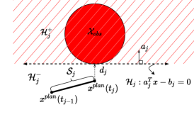
Figure 1: The least conservative hyperplane $\mathcal{H}_{j}$ approximating $\mathcal{X}_{obs}$ (shown in a red-faced circle) with a half space $\mathcal{H}_{j}^{+}$ (shown in red hatching). $d_{j}$ is the minimum distance of $\mathcal{S}_{j}$ from $\mathcal{X}_{obs}$.

Now, it can be shown that

$$\left(\bigcup\limits_{t\in\mathcal{T}_{j}}\boldsymbol{x}^{sys}(t)\in\mathcal{H}_{j}^{+}\!\!\right)\subseteq\left(\bigcup\limits_{t\in\mathcal{T}_{j}}a_{j}^{T}\boldsymbol{x}(t)\geq d_{j}\!\right)$$ (18)

where $\boldsymbol{x}(t)$ is the deviation of the robot from the planned trajectory as defined in (11). Proof of (18) is presented in Appendix A. Using (16) and (18), $\mathcal{R}$ can be upper-bounded as

$$\mathcal{R}\leq\!P\left(\bigcup\limits_{j=1}^{N}\bigcup\limits_{t\in\mathcal{T}_{j}}a_{j}^{T}\boldsymbol{x}(t)\geq d_{j}\right).$$ (19)

For the proposed robot dynamics (Section II-B), it is trivial to show that $a_{j}^{T}\boldsymbol{x}(t)$ is a one-dimensional Brownian motion for $t\in[0,T]$ that starts in the origin. Let us denote $\boldsymbol{w}_{j}(t)\coloneqq a_{j}^{T}\boldsymbol{x}(t)$, $j=1,2,\ldots,N$. Now, (19) can be written as

$$\mathcal{R}\leq P\left(\bigcup\limits_{j=1}^{N}\;\underset{t\in\mathcal{T}_{j}}{\text{max}}\;\boldsymbol{w}_{j}(t)\geq d_{j}\right).$$ (20)

Defining $\mathcal{E}_{j}\coloneqq\left(\underset{t\in\mathcal{T}_{j}}{\text{max}}\;\boldsymbol{w}_{j}(t)\geq d_{j}\right)$, (20) can be rewritten as

$$\mathcal{R}\leq P\left(\bigcup\limits_{j=1}^{N}\mathcal{E}_{j}\right).$$ (21)

Since $\{\mathcal{E}_{j}\}_{j=1,2,\ldots,N}$ are non-independent events, computing (21) exactly is a challenging task. In the following sections, we derive bounds for $P\left(\bigcup\limits_{j=1}^{N}\mathcal{E}_{j}\right)$.

III-B First-Order Risk Bound

Define $p_{j}\coloneqq P(\mathcal{E}_{j})=P\left(\underset{t\in[t_{j-1},t_{j}]}{\text{max}}\boldsymbol{w}_{j}(t)\geq d_{j}\right)$. Applying Boole’s inequality (3), the probability in (21) can be decomposed as

$$\mathcal{R}\leq P\left(\bigcup\limits_{j=1}^{N}\mathcal{E}_{j}\right)\leq\sum\limits_{j=1}^{N}p_{j}.$$ (22)

This gives us a first-order risk bound for $\mathcal{R}$. $p_{j}$ is the continuous-time risk associated with the time segment $\mathcal{T}_{j}=[t_{j-1},t_{j}]$. Note that the bound in (22) possesses the time-additive structure which is helpful to use this bound in the risk-aware motion planning algorithms.

In order to take advantage of the reflection principle to compute $p_{j}$, Ariu et al. [15] proposes to compute an upper bound to $p_{j}$ as

$$p_{j}\leq P\left(\underset{t\in[0,t_{j}]}{\text{max}}\,\boldsymbol{w}_{j}(t)\geq d_{j}\right).$$ (23)

Using the reflection principle (14), the right side of (23) can be evaluated as

$$\!\!P\!\left(\!\underset{t\in[0,t_{j}]}{\text{max}}\!\boldsymbol{w}_{j}(t)\!\geq\!d_{j}\!\!\right)\!\!=\!2P\!\left(\boldsymbol{w}_{j}(t_{j})\!\geq\!d_{j}\!\right)\!=\!2P\!\left(\!a_{j}^{T}\boldsymbol{x}_{j}\!\geq\!d_{j}\!\right)\!.$$ (24)

From (22), (23), and (24) we get

$$\mathcal{R}\leq 2\sum\limits_{j=1}^{N}P\left(a_{j}^{T}\boldsymbol{x}_{j}\geq d_{j}\right).$$ (25)

The bound in (25) requires computing probabilities only at the discrete-time steps, simplifying the estimation of the continuous-time risk. However, the over-approximation in (23) introduces unnecessary conservatism that can be avoided using the Markov property of Brownian motion. Next, we present a way by which $p_{j}$ can be computed exactly without any over-approximation.

For notational convenience, let us denote the random variables $\boldsymbol{w}_{j}(t_{j-1})$ and $\boldsymbol{w}_{j}(t_{j})$ by $\boldsymbol{z}^{s}_{j}$ and $\boldsymbol{z}^{e}_{j}$ respectively:

$$\boldsymbol{z}^{s}_{j}\coloneqq\boldsymbol{w}_{j}(t_{j-1})=a_{j}^{T}\boldsymbol{x}_{j-1},\quad\boldsymbol{z}^{e}_{j}\coloneqq\boldsymbol{w}_{j}(t_{j})=a_{j}^{T}\boldsymbol{x}_{j}$$ (26)

for $j=1,2,\ldots,N$. If $\mu_{\boldsymbol{\xi}}(\xi)$ denotes the probability density function (p.d.f.) of any random variable $\boldsymbol{\xi}$, then

$$\mu_{\boldsymbol{z}^{s}_{j}}({z}^{s}_{j})=\mathcal{N}(0,\sigma_{\boldsymbol{z}^{s}_{j}}^{2}), \qquad\sigma_{\boldsymbol{z}^{s}_{j}}^{2}=a_{j}^{T}\Sigma_{\boldsymbol{x}_{j-1}}a_{j},$$ (27)

$$\mu_{\boldsymbol{z}^{e}_{j}}({z}^{e}_{j})=\mathcal{N}(0,\sigma_{\boldsymbol{z}^{e}_{j}}^{2}), \qquad\sigma_{\boldsymbol{z}^{e}_{j}}^{2}=a_{j}^{T}\Sigma_{\boldsymbol{x}_{j}}a_{j}.$$

Let us define $\boldsymbol{z}_{j}\coloneqq\begin{bmatrix}\boldsymbol{z}^{s}_{j}&\boldsymbol{z}^{e}_{j}\end{bmatrix}^{T}\in\mathbb{R}^{2}$. It is straightforward to show that the joint distribution of $\boldsymbol{z}_{j}$ is

$$\mu_{\boldsymbol{z}_{j}}({z}_{j})=\mathcal{N}\left(0,\Sigma_{\boldsymbol{z}_{j}}\right),\qquad\Sigma_{\boldsymbol{z}_{j}}=\begin{bmatrix}\sigma_{\boldsymbol{z}^{s}_{j}}^{2}&\sigma_{\boldsymbol{z}^{s}_{j}}^{2}\\ \sigma_{\boldsymbol{z}^{s}_{j}}^{2}&\sigma_{\boldsymbol{z}^{e}_{j}}^{2}\end{bmatrix}.$$ (28)

Now, we compute $p_{j}$ using the following theorem:

Theorem 2

If $\mu_{\boldsymbol{z}^{s}_{j}}({z}^{s}_{j})$ and $\mu_{\boldsymbol{z}_{j}}({z}_{j})$ are the distributions of the normal random variables $\boldsymbol{z}^{s}_{j}$ and $\boldsymbol{z}_{j}$, represented as (27) and (28) respectively, then $p_{j}$ is given by:

$$p_{j}\!=\!\!\!\int_{{z}_{j}^{s}=d_{j}}^{\infty}\!\!\!\!\!\mu_{\boldsymbol{z}^{s}_{j}}({z}^{s}_{j})d{z}_{j}^{s}\!+2\!\!\int_{{z}_{j}^{s}=-\infty}^{d_{j}}\!\int_{{z}_{j}^{e}=d_{j}}^{\infty}\!\!\!\!\mu_{\boldsymbol{z}_{j}}({z}_{j})d{z}_{j}^{e}d{z}_{j}^{s}.$$ (29)

Proof:

Let us define:

$$p_{j}^{1}\coloneqq P\left(\underset{t\in[t_{j-1},t_{j}]}{\text{max}}\boldsymbol{w}_{j}(t)\geq d_{j},\;\boldsymbol{w}_{j}(t_{j-1})\geq d_{j}\right),$$

$$p_{j}^{2}\coloneqq P\left(\underset{t\in[t_{j-1},t_{j}]}{\text{max}}\boldsymbol{w}_{j}(t)\geq d_{j},\;\boldsymbol{w}_{j}(t_{j-1})<d_{j}\right).$$

Using the law of total probability, we can write $p_{j}$ as

$$p_{j}=p_{j}^{1}+p_{j}^{2}.$$ (30)

Since $\left(\boldsymbol{w}_{j}(t_{j-1})\geq d_{j}\right)\subseteq\left(\underset{t\in[t_{j-1},t_{j}]}{\text{max}}\boldsymbol{w}_{j}(t)\geq d_{j}\right)$, $p_{j}^{1}$ can be computed as

$$p_{j}^{1}=P\left(\boldsymbol{w}_{j}(t_{j-1})\geq d_{j}\right)=\int_{{z}_{j}^{s}=d_{j}}^{\infty}\mu_{\boldsymbol{z}^{s}_{j}}({z}^{s}_{j})d{z}_{j}^{s}.$$ (31)

Now, we write $p_{j}^{2}$ as

$$p_{j}^{2}= P\left(\underset{t\in[t_{j-1},t_{j}]}{\text{max}}\boldsymbol{w}_{j}(t)\geq d_{j},\;\boldsymbol{z}_{j}^{s}<d_{j}\right)$$

$$= P\left(\underset{t\in[0,t_{j}-t_{j-1}]}{\text{max}}\boldsymbol{w}_{j}(t+t_{j-1})\geq d_{j},\;\boldsymbol{z}_{j}^{s}<d_{j}\right).$$

From Markov property of Brownian motion (Definition 1),

$$\widetilde{\boldsymbol{w}}_{j}(t)=\boldsymbol{w}_{j}(t+t_{j-1})-\boldsymbol{w}_{j}(t_{j-1}),\quad t\in[0,(T-t_{j-1})]$$ (32)

is a one-dimensional Brownian motion that starts in the origin. Rewriting $p_{j}^{2}$ in terms of $\widetilde{\boldsymbol{w}}_{j}(t)$, we get

$$p_{j}^{2} =P\left(\underset{t\in[0,t_{j}-t_{j-1}]}{\text{max}}\widetilde{\boldsymbol{w}}_{j}(t)\geq d_{j}-\boldsymbol{z}_{j}^{s},\;\boldsymbol{z}_{j}^{s}<d_{j}\right)$$ (33)

$$=\!\!\!\int_{-\infty}^{d_{j}}\!\!\!P\!\left(\underset{t\in[0,t_{j}-t_{j-1}]}{\text{max}}\!\widetilde{\boldsymbol{w}}_{j}(t)\!\geq\!d_{j}-{z}_{j}^{s}\right)\mu_{\boldsymbol{z}^{s}_{j}}({z}^{s}_{j})d{z}_{j}^{s}.$$

Since $d_{j}-{z}_{j}^{s}>0$, $\forall\,{z}_{j}^{s}\in(-\infty,d_{j})$, we can apply the reflection principle (14) and rewrite (33) as

$$p_{j}^{2}\!=\!\!\int_{-\infty}^{d_{j}}\!\!\!2P\!\left(\widetilde{\boldsymbol{w}}_{j}(t_{j}\!-\!t_{j-1})\geq d_{j}\!-\!{z}_{j}^{s}\right)\mu_{\boldsymbol{z}^{s}_{j}}({z}^{s}_{j})d{z}_{j}^{s}.$$ (34)

Let us denote the random variable $\widetilde{\boldsymbol{w}}_{j}(t_{j}-t_{j-1})$ by $\boldsymbol{y}_{j}$. Using (32) and (26),

$$\boldsymbol{y}_{j}\coloneqq\widetilde{\boldsymbol{w}}_{j}(t_{j}-t_{j-1})=\boldsymbol{w}_{j}(t_{j})-\boldsymbol{w}_{j}(t_{j-1})=\boldsymbol{z}_{j}^{e}-\boldsymbol{z}_{j}^{s},$$

and the p.d.f. of $\boldsymbol{y}_{j}$ is $\mu_{\boldsymbol{y}_{j}}({y}_{j})=\mathcal{N}(0,\sigma_{\boldsymbol{y}_{j}}^{2})$ where $\sigma_{\boldsymbol{y}_{j}}^{2}=\sigma_{\boldsymbol{z}^{e}_{j}}^{2}-\sigma_{\boldsymbol{z}^{s}_{j}}^{2}$. Now, (34) can be rewritten as

$$p_{j}^{2} =2\int_{-\infty}^{d_{j}}\left(\int_{d_{j}-{z}_{j}^{s}}^{\infty}\mu_{\boldsymbol{y}_{j}}({y}_{j})\,d{y}_{j}\right)\mu_{\boldsymbol{z}^{s}_{j}}({z}^{s}_{j})d{z}_{j}^{s}$$ (35)

$$\!\!\!\!\!\!\!\!\!\!\!\!\!\!=\!2\!\!\!\int_{\!\!-\infty}^{d_{j}}\!\!\int_{\!d_{j}-{z}_{j}^{s}}^{\infty}\!\frac{1}{2\pi\sigma_{\boldsymbol{z}_{j}^{s}}\sigma_{\boldsymbol{y}_{j}}}exp\!\!\left\{\!\!-\frac{1}{2}\!\!\left(\!\!\frac{{z}_{j}^{s}}{\sigma_{\boldsymbol{z}_{j}^{s}}}\!\!\right)^{\!\!\!2}\!\!-\!\frac{1}{2}\!\!\left(\!\!\frac{{y}_{j}}{\sigma_{\boldsymbol{y}_{j}}}\!\!\right)^{\!\!\!2}\!\!\right\}\!\!d{y}_{j}d{z}_{j}^{s}.$$

The outside integral in right side of (35) is w.r.t. ${z}_{j}^{s}$ and the inside is one is w.r.t. ${y}_{j}$. Substituting ${y}_{j}$ with ${z}_{j}^{e}-{z}_{j}^{s}$, (35) can be rewritten as

$$p_{j}^{2}= 2\!\!\int_{{z}_{j}^{s}=-\infty}^{d_{j}}\!\int_{{z}_{j}^{e}=d_{j}}^{\infty}\frac{1}{2\pi\sigma_{\boldsymbol{z}_{j}^{s}}\sigma_{\boldsymbol{z}_{j}^{e}}\sqrt{1-\rho^{2}}}\cdot$$ (36)

$$\!\!\!\!\!\!\!\!\!\!\!\!\!\!\!\!\!\!\!\!\!\!\!\!exp\!\left\{\!\!-\frac{1}{2\!\left(1\!-\!\rho^{2}\right)}\!\!\left[\left(\!\!\frac{{z}_{j}^{s}}{\sigma_{\boldsymbol{z}_{j}^{s}}}\!\!\right)^{\!\!\!2}\!\!-\frac{2\rho\,{z}_{j}^{s}{z}_{j}^{e}}{\sigma_{\boldsymbol{z}_{j}^{s}}\sigma_{\boldsymbol{z}_{j}^{e}}}+\!\!\left(\!\!\frac{{z}_{j}^{e}}{\sigma_{\boldsymbol{z}_{j}^{e}}}\!\!\right)^{\!\!\!2}\right]\right\}d{z}_{j}^{e}\,d{z}_{j}^{s}$$

where $\rho=\sigma_{\boldsymbol{z}_{j}^{s}}/\sigma_{\boldsymbol{z}_{j}^{e}}$. The expression inside the double integral of (36) is a bivariate normal distribution of $\boldsymbol{z}_{j}$. Hence,

$$p_{j}^{2}=2\!\!\int_{{z}_{j}^{s}=-\infty}^{d_{j}}\int_{{z}_{j}^{e}=d_{j}}^{\infty}\mu_{\boldsymbol{z}_{j}}({z}_{j})d{z}_{j}^{e}\,d{z}_{j}^{s}.$$ (37)

Combining (30), (31) and (37) we recover (29). ∎

MATLAB’s mvncdf function can be utilized to compute the integrations (31) and (37) numerically.

III-C Second-Order Risk Bound

The proposed first-order risk bound (22) can be tightened using a variant of Hunter’s inequality that additionally considers the joint probability of consecutive events [23]:

$$\mathcal{R}\leq P\left(\bigcup\limits_{j=1}^{N}\mathcal{E}_{j}\right)\leq\sum\limits_{j=1}^{N}p_{j}-\sum\limits_{j=1}^{N-1}p_{j,\,j+1}$$

where $p_{j,\,j+1}\coloneqq P(\mathcal{E}_{j}\cap\mathcal{E}_{j+1})$ is the joint risk associated with the time segments $\mathcal{T}_{j}$ and $\mathcal{T}_{j+1}$. Computing $p_{j,\,j+1}$ exactly is challenging. In this work, we propose to compute a lower bound $p_{j,\,j+1}^{LB}$ of $p_{j,\,j+1}$ using the following theorem:

Theorem 3

If $t_{j-1}=\hat{t}_{j}^{0}<\hat{t}_{j}^{1}<\ldots<\hat{t}_{j}^{r_{j}}=t_{j}$ is a discretization of the time segment $\mathcal{T}_{j}$, and $\boldsymbol{z}_{j}^{i}$, $\mathcal{D}_{j}$ are defined as

$$\boldsymbol{z}_{j}^{i}\coloneqq\boldsymbol{w}_{j}(\hat{t}_{j}^{i})=a_{j}^{T}\boldsymbol{x}(\hat{t}_{j}^{i}),$$

$$\mathcal{D}_{j}\coloneqq\left(\boldsymbol{z}_{j}^{0}<d_{j}\right)\cap\left(\boldsymbol{z}_{j}^{1}<d_{j}\right)\cap\ldots\cap\left(\boldsymbol{z}_{j}^{r_{j}}<d_{j}\right),$$

then $p_{j,\,j+1}$ is lower bounded by $p_{j,\,j+1}^{LB}$ given as

$$p_{j,\,j+1}^{LB}=1-P(\mathcal{D}_{j})-P(\mathcal{D}_{j+1})+P(\mathcal{D}_{j}\cap\mathcal{D}_{j+1}).$$

Proof:

Introduce $\mathcal{C}_{j}$ as

$$\mathcal{C}_{j}= \left(\boldsymbol{w}_{j}(\hat{t}_{j}^{0})\geq d_{j}\right)\cup\left(\boldsymbol{w}_{j}(\hat{t}_{j}^{1})\geq d_{j}\right)\cup\ldots\cup\left(\boldsymbol{w}_{j}(\hat{t}_{j}^{r_{j}})\geq d_{j}\right)$$

$$= \left(\boldsymbol{z}_{j}^{0}\geq d_{j}\right)\cup\left(\boldsymbol{z}_{j}^{1}\geq d_{j}\right)\cup\ldots\cup\left(\boldsymbol{z}_{j}^{r_{j}}\geq d_{j}\right)$$

$$= \mathcal{D}_{j}^{c}.$$

Now, since $\mathcal{C}_{j}\subset\mathcal{E}_{j}$

$$p_{j,\,j+1} \geq P(\mathcal{C}_{j}\cap\mathcal{C}_{j+1})$$

$$=1-P(\mathcal{D}_{j}\cup\mathcal{D}_{j+1})$$

$$=1-P(\mathcal{D}_{j})-P(\mathcal{D}_{j+1})+P(\mathcal{D}_{j}\cap\mathcal{D}_{j+1})$$

$$=p_{j,\,j+1}^{LB}.$$

∎

$P(\mathcal{D}_{j})$ can be computed by finding the joint distribution of $\begin{bmatrix}\boldsymbol{z}_{j}^{0}&\boldsymbol{z}_{j}^{1}&\ldots&\boldsymbol{z}_{j}^{r_{j}}\end{bmatrix}^{T}$ and $P(\mathcal{D}_{j}\cap\mathcal{D}_{j+1})$ by finding the joint distribution of $\begin{bmatrix}\boldsymbol{z}_{j}^{0}&\boldsymbol{z}_{j}^{1}&\ldots&\boldsymbol{z}_{j}^{r_{j}}&\boldsymbol{z}_{j+1}^{0}&\boldsymbol{z}_{j+1}^{1}&\ldots&\boldsymbol{z}_{j+1}^{r_{j+1}}\end{bmatrix}^{T}$. The computations of $P(\mathcal{D}_{j})$ and $P(\mathcal{D}_{j}\cap\mathcal{D}_{j+1})$ are summarized in Appendix B. Now, we get our second-order risk bound as follows:

$$\mathcal{R}\leq\sum\limits_{j=1}^{N}p_{j}-\sum\limits_{j=1}^{N-1}p_{j,\,j+1}^{LB}.$$ (38)

Similar to the first-order risk bound (22), this bound also possesses the time-additive structure. Note that the higher sampling rates we choose to discretize the time segments $\mathcal{T}_{j}$ (a set of higher $r_{j}$’s), the tighter the bound in (38) becomes.

III-D Risk Analysis when $\mathcal{X}_{obs}$ is Non-Convex

As mentioned earlier, the analysis in Sections III-A to III-C assumes that $\mathcal{X}_{obs}$ is convex, which is sufficient to guarantee the existence of a set of separating hyperplanes $\{\mathcal{H}_{j}\}_{j=1,2,\ldots,N}$. When $\mathcal{X}_{obs}$ is non-convex, we partition it into $M$ subregions $\mathcal{X}_{obs_{m}}$, $m=1,2,\ldots,M$ such that $\mathcal{X}_{obs}=\left(\bigcup\limits_{m=1}^{M}\mathcal{X}_{obs_{m}}\right)$ and a set of separating hyperplanes $\{\mathcal{H}_{j}\}_{j=1,2,\ldots,N}$ exists for each $\mathcal{X}_{obs_{m}}$. We then bound $\mathcal{R}$ as

$$\mathcal{R}\leq\sum\limits_{m=1}^{M}\mathcal{R}_{m},\qquad\mathcal{R}_{m}=P\left(\bigcup\limits_{t\in[0,T]}\boldsymbol{x}^{sys}(t)\in\mathcal{X}_{obs_{m}}\right).$$

The first and second-order upper bounds for $\mathcal{R}_{m}$ can be computed using the analysis in Sections III-A to III-C. In order to obtain tight upper-bounds for $\mathcal{R}$, the partitioning of $\mathcal{X}_{obs}$ can be optimized which is left for the future work.

IV Simulation Results

In this Section, we demonstrate the validity and performance of our continuous-time risk bounds via a ground robot navigation simulation. The configuration space is $\mathcal{X}=[0,1]\times[0,1]$. We assume that the robot dynamics are governed by the Itô process (6), with $R=10^{-3}\times I$ ($I$ is a $2\times 2$ identity matrix), and it is commanded to travel at a unit velocity i.e., $\|\boldsymbol{v}^{sys}(t)\|=1$, $t\in[0,T]$. As explained in Section II, we discretize the dynamics (6) under the time partition $\mathcal{T}$. Due to the unit velocity assumption, $\Delta t_{j}=\|x_{j+1}^{plan}-x_{j}^{plan}\|$. Hence, our discrete-time robot dynamics are

$$\boldsymbol{x}^{sys}_{j+1}\!\!=\!\boldsymbol{x}^{sys}_{j}\!\!+\boldsymbol{u}^{sys}_{j}\!\!+\boldsymbol{n}_{j},\quad\boldsymbol{n}_{j}\!\sim\!\mathcal{N}(0,\|x_{j+1}^{plan}-x_{j}^{plan}\|R),$$ (39)

where $\boldsymbol{u}_{j}^{sys}$ is defined as per (10). The model (39) is natural for ground robots whose location uncertainty grows linearly with the distance traveled.

First, we plan trajectories using RRT* with the instantaneous safety criterion [24] (i.e., at every time step, the confidence ellipse with a fixed safety level is collision-free). For a given configuration space, four planned trajectories with $95\%$, $75\%$, $50\%$, and $25\%$ instantaneous safety levels are shown in Fig. 2. In each case, the confidence ellipses grow in size with the distance since the robot tracks these trajectories in open-loop.

	​​​​​​​
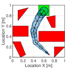
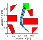
(a)	(b)
	​​​​​​​
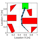
(c)	(d)

Figure 2: Trajectories planned with the instantaneous safety criterion [24] are shown in black. The black dots on the trajectories represent the planned positions $\{x^{plan}_{j}\}_{j=1,2,\ldots,N}$. The red dot represents the initial position $x^{plan}_{0}$ of the robot. The red-faced polygons represent $\mathcal{X}_{obs}$ and the green faced rectangle represents $\mathcal{X}_{goal}$. The trajectories are shown with (a) $95\%$, (b) $75\%$, (c) $50\%$ and (d) $25\%$ confidence ellipses. The ellipses at the time steps $\{t_{j}\}_{j=1,2,\ldots,N}$ are shown in black and the ellipses at the intermediate time steps are shown in blue.

Fig. 3 plots the continuous and discrete-time risk bounds for these plans having different instantaneous safety (risk) levels. For validation, we compute failure probabilities using $10^{5}$ Monte Carlo simulations at a high rate of time discretization ($r_{d}=100$) and assume them as the ground truths (shown in black). The dotted graphs are the discrete-time risk bounds ($B_{d}$) computed using (4) at different rates of time discretization ($r_{d}$). As is evident from the graph, the discrete-time risk bounds at a lower rate of time discretization underestimate the Monte Carlo estimates, and as the time-discretization rate increases, they become overly conservative. On the other hand, our continuous-time risk bounds ($B_{c}$) (shown with solid red and blue graphs) are tighter, and at the same time ensure conservatism.

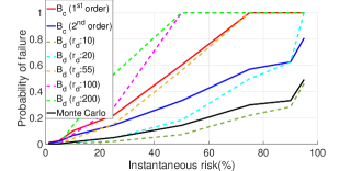
Figure 3: End-to-end probabilities of failure computed for the trajectories with different instantaneous risk levels. The solid red and blue graphs represent the first-order and second-order continuous-time risk bounds ($B_{c}$) respectively. The dotted graphs are discrete-time risk bounds ($B_{d}$) computed using (4) at different rates of time discretization ($r_{d}$). The Monte Carlo estimates of the same trajectories are shown in black.

Next, we demonstrate a larger statistical evaluation over $100$ trajectories planned using RRT* in randomly-generated environments (random initial, goal and obstacle positions). These trajectories are generated with $5\%$ instantaneous safety criterion [24]. The average risk estimate of $10^{5}$ Monte Carlo simulations (run at a high rate of time discretization $r_{d}=100$) is $0.27$. The statistics of the discrete-time and continuous-time risk estimates are shown in Table I. The discrete-time risk estimates are computed using (4) at increasing rates of time discretization ($r_{d}$). The continuous-time risk estimates are computed using the method proposed by Ariu et al. [15] and our approach. The Bias and RMSE columns lists respectively the mean (signed) difference and the root mean squared difference between the corresponding estimate and the Monte Carlo estimate. The % Conservative column reports the percentage of cases where the corresponding estimate was greater than (or within 0.1% of) the Monte Carlo estimate and the Avg. Time lists the average computation times for our MATLAB implementations.

TABLE I: Comparison of different risk estimates over $100$ trajectories. Computation is performed in MATLAB on a consumer laptop.

Risk Estimates	Avg. Time	Bias	RMSE	%Conservative
Monte Carlo	101.50 s	0	0	-
Discrete-time
$r_{d}:5$	0.14 s	-0.14	0.18	28%
$r_{d}:10$	0.26 s	-0.002	0.16	59%
$r_{d}:20$	0.52 s	0.31	0.57	82%
$r_{d}:55$	1.53 s	1.50	2.33	100%
$r_{d}:100$	2.87 s	2.98	4.53	100%
Continuous-time
Ariu et al. [15]	1.39 s	0.97	1.33	100%
Our $1^{st}$ order	1.47 s	0.66	0.90	100%
Our $2^{nd}$ order	2.23 s	0.28	0.36	100%

From the data presented, following conclusions can be drawn: First, our risk bounds require significantly less computation time than the Monte Carlo method. Second, unlike the discrete-time risk bounds at the lower sampling rates, our bounds remain conservative (i.e., safe) in all the trials. Lastly, our bounds produce tighter estimates than the discrete-time risk bounds at the higher sampling rates and the continuous-time risk bound of [15].

V Conclusion

In this paper, we conducted an analysis to estimate the continuous-time collision probability of motion plans for autonomous agents with linear controlled Itô dynamics. We derived two upper bound for the continuous-time risk using the properties of Brownian motion (Markov property and reflection principle), and probability inequalities (Boole and Hunter’s inequality). Our method boils down to computing probabilities at the discrete-time steps, simplifying the analysis, yet providing risk guarantees in continuous-time. We show that our bounds outperform the discrete-time risk bound (4) and are cheaper in computation than the naïve Monte Carlo sampling method.

Our analysis motivates a number of future investigations. This paper assumes that the robot follows a linear controlled Itô process. Future work will focus on risk analysis for systems with generalized stochastic dynamics. Another direction we would like to explore is risk analysis by fusing sampling-based methods and methods from continuous stochastic processes as suggested in [14]. This hybrid approach may provide the best of both worlds: high accuracy as well as computational simplicity and compatibility with continuous optimization.

APPENDIX A

Proof of (18)

$$\left(\bigcup\limits_{t\in\mathcal{T}_{j}}\boldsymbol{x}^{sys}(t)\in\mathcal{H}_{j}^{+}\!\!\right) =\left(\bigcup\limits_{t\in\mathcal{T}_{j}}a_{j}^{T}\boldsymbol{x}^{sys}(t)\geq b_{j}\right)$$ (40)

$$\!\!\!\!\!\!\!\!\!\!\!\!\!\!\!\!\!\!\!\!\!\!\!\!\!\!=\left(\bigcup\limits_{t\in\mathcal{T}_{j}}a_{j}^{T}\boldsymbol{x}(t)\geq b_{j}-a_{j}^{T}x^{plan}(t)\right).$$

Two equalities of (40) follow from (15) and (11) respectively. Now, recall that $d_{j}$ is the minimum distance of $\mathcal{S}_{j}$ from $\mathcal{X}_{obs}$ i.e., $d_{j}=b_{j}-a_{j}^{T}y_{2}^{*}$, where $y_{2}^{*}$ is the solution to the optimization problem (17). Noting that $b_{j}-a_{j}^{T}x^{plan}(t)\geq d_{j}$, $\forall\,t\in\mathcal{T}_{j}$, from (40),

$$\left(\bigcup\limits_{t\in\mathcal{T}_{j}}\boldsymbol{x}^{sys}(t)\in\mathcal{H}_{j}^{+}\!\!\right)\subseteq\left(\bigcup\limits_{t\in\mathcal{T}_{j}}a_{j}^{T}\boldsymbol{x}(t)\geq d_{j}\!\right).$$

APPENDIX B

Computation of $P(\mathcal{D}_{j})$ and $P(\mathcal{D}_{j}\cap\mathcal{D}_{j+1})$

Let us define: $\Delta\hat{t}_{j}^{i}\coloneqq\hat{t}_{j}^{i+1}-\hat{t}_{j}^{i}$, and $\hat{\boldsymbol{x}}_{j}^{i}\coloneqq\boldsymbol{x}(\hat{t}_{j}^{i})$. From (12), we can write

$$\hat{\boldsymbol{x}}_{j}^{i+1}=\hat{\boldsymbol{x}}_{j}^{i}+\hat{\boldsymbol{n}}_{j}^{i},\qquad\hat{\boldsymbol{n}}_{j}^{i}\sim\mathcal{N}(0,\Sigma_{\hat{\boldsymbol{n}}_{j}^{i}})$$ (41)

where $\hat{\boldsymbol{x}}_{j}^{0}=\boldsymbol{x}_{j-1}$, $\Sigma_{\hat{\boldsymbol{n}}_{j}^{i}}\coloneqq\Delta\hat{t}_{j}^{i}R$, for $i=0,1,\ldots,r_{j}-1$, and $j=1,2,\ldots,N$. Multiplying both sides of (41) by $a_{j}^{T}$ we get

$$a_{j}^{T}\hat{\boldsymbol{x}}_{j}^{i+1}=\boldsymbol{z}^{i+1}_{j}=a_{j}^{T}\hat{\boldsymbol{x}}_{j}^{i}+a_{j}^{T}\hat{\boldsymbol{n}}_{j}^{i},\qquad\hat{\boldsymbol{n}}_{j}^{i}\sim\mathcal{N}(0,\Sigma_{\hat{\boldsymbol{n}}_{j}^{i}}).$$

Stacking all $\boldsymbol{z}_{j}^{i}$ for $i=0,1,\ldots,r_{j}$, we can write the dynamics for the entire time segment $\mathcal{T}_{j}$ as

$$\boldsymbol{z}_{j}^{seg}=M_{j}\hat{\boldsymbol{x}}_{j}^{0}+K_{j}\hat{\boldsymbol{n}}_{j}^{seg},\qquad\hat{\boldsymbol{n}}_{j}^{seg}\sim\mathcal{N}(0,\Sigma_{\hat{\boldsymbol{n}}_{j}^{seg}})$$ (42)

where $\boldsymbol{z}_{j}^{seg}\coloneqq\begin{bmatrix}\boldsymbol{z}_{j}^{0}&\boldsymbol{z}_{j}^{1}&\ldots&\boldsymbol{z}_{j}^{r_{j}}\end{bmatrix}^{T}$, $M_{j}=a_{j}^{T}\cdot\mathds{1}$,
$\hat{\boldsymbol{n}}_{j}^{seg}=\begin{bmatrix}\hat{\boldsymbol{n}}_{j}^{0}&\hat{\boldsymbol{n}}_{j}^{1}&\ldots&\hat{\boldsymbol{n}}_{j}^{r_{j}-1}\end{bmatrix}^{T},\quad\Sigma_{\hat{\boldsymbol{n}}_{j}^{seg}}=\underset{0\leq i\leq r_{j}-1}{\text{diag}}\Sigma_{\hat{\boldsymbol{n}}_{j}^{i}},$

$$K_{j}=\begin{bmatrix}0&0&\ldots&0\\ a_{j}^{T}&0&\ldots&0\\ a_{j}^{T}&a_{j}^{T}&\ldots&0\\ \vdots&\vdots&\ddots&\vdots\\ a_{j}^{T}&a_{j}^{T}&\ldots&a_{j}^{T}\end{bmatrix}$$

Computation of $P(\mathcal{D}_{j})$:

In order to compute $P(\mathcal{D}_{j})$, we need to find the distribution of $\boldsymbol{z}_{j}^{seg}$. Since $\hat{\boldsymbol{x}}_{j}^{0}=\boldsymbol{x}_{j-1}$, it is distributed as $\hat{\boldsymbol{x}}_{j}^{0}\sim\mathcal{N}(0,\Sigma_{\boldsymbol{x}_{j-1}})$. Hence, from (42), the p.d.f. of $\boldsymbol{z}_{j}^{seg}$ can be written as $\mu_{\boldsymbol{z}_{j}^{seg}}({z}_{j}^{seg})=\mathcal{N}(0,\Sigma_{\boldsymbol{z}_{j}^{seg}})$ where $\Sigma_{\boldsymbol{z}_{j}^{seg}}=M_{j}\Sigma_{\boldsymbol{x}_{j-1}}M_{j}^{T}+K_{j}\Sigma_{\hat{\boldsymbol{n}}_{j}^{seg}}K_{j}^{T}$. Now, $P(\mathcal{D}_{j})$ can be computed as

$$P(\mathcal{D}_{j})=\int_{\mathcal{C}_{j}}\mu_{\boldsymbol{z}_{j}^{seg}}({z}_{j}^{seg})\,d{z}_{j}^{seg}$$ (43)

where $\mathcal{C}_{j}$ is a hypercube of dimension $r_{j}+1$, having its sides along each direction run from $-\infty$ to $d_{j}$.

Computation of $P(\mathcal{D}_{j}\cap\mathcal{D}_{j+1})$:

Let us define $\boldsymbol{z}_{j,\,j+1}^{seg}\coloneqq\begin{bmatrix}\boldsymbol{z}_{j}^{seg}&\boldsymbol{z}_{j+1}^{seg}\end{bmatrix}^{T}$. In order to compute $P(\mathcal{D}_{j}\cap\mathcal{D}_{j+1})$, we need to find the distribution of $\boldsymbol{z}_{j,\,j+1}^{seg}$. First, let us write $\hat{\boldsymbol{x}}_{j+1}^{0}$ in terms of $\hat{\boldsymbol{x}}_{j}^{0}$.

$$\hat{\boldsymbol{x}}_{j+1}^{0}=\hat{\boldsymbol{x}}_{j}^{0}+G_{j}\hat{\boldsymbol{n}}_{j}^{seg}$$ (44)

where $G_{j}=\begin{bmatrix}I&I&\ldots&I\end{bmatrix}_{n\times nr_{j}}$, $j=1,2,\ldots,N-1,$ and $I$ is an $n\times n$ identity matrix. We know that

$$\boldsymbol{z}_{j+1}^{seg}=M_{j+1}\hat{\boldsymbol{x}}_{j+1}^{0}+K_{j+1}\hat{\boldsymbol{n}}_{j+1}^{seg}.$$ (45)

Substituting $\hat{\boldsymbol{x}}_{j+1}^{0}$ from (44) in (45), we get

$$\boldsymbol{z}_{j+1}^{seg}=M_{j+1}\hat{\boldsymbol{x}}_{j}^{0}+M_{j+1}G_{j}\hat{\boldsymbol{n}}_{j}^{seg}+K_{j+1}\hat{\boldsymbol{n}}_{j+1}^{seg}.$$ (46)

Let $H_{j,\,j+1}\coloneqq cov(\boldsymbol{z}_{j}^{seg},\;\boldsymbol{z}_{j+1}^{seg})$. Using (42) and (46), we can show that

$$H_{j,\,j+1}=M_{j}\Sigma_{\boldsymbol{x}_{j-1}}M_{j+1}^{T}+K_{j}\Sigma_{\hat{\boldsymbol{n}}_{j}^{seg}}G_{j}^{T}M_{j+1}^{T}.$$ (47)

For computing (47) we use the fact that

$$cov(\hat{\boldsymbol{x}}_{j}^{0},\hat{\boldsymbol{n}}_{j}^{seg})=cov(\hat{\boldsymbol{x}}_{j}^{0},\hat{\boldsymbol{n}}_{j+1}^{seg})=cov(\hat{\boldsymbol{n}}_{j}^{seg},\hat{\boldsymbol{n}}_{j+1}^{seg})=0$$

Now, the p.d.f. of $\boldsymbol{z}_{j,\,j+1}^{seg}$ can be written as $\mu_{\boldsymbol{z}_{j,\,j+1}^{seg}}\left({z}_{j,\,j+1}^{seg}\right)=\mathcal{N}(0,\Sigma_{\boldsymbol{z}_{j,\,j+1}^{seg}})$ where

$$\Sigma_{\boldsymbol{z}_{j,\,j+1}^{seg}}=\begin{bmatrix}\Sigma_{\boldsymbol{z}_{j}^{seg}}&H_{j,\,j+1}\\ H_{j,\,j+1}^{T}&\Sigma_{\boldsymbol{z}_{j+1}^{seg}}\end{bmatrix}$$

and $P(\mathcal{D}_{j}\cap\mathcal{D}_{j+1})$ can be computed as

$$P(\mathcal{D}_{j}\cap\mathcal{D}_{j+1})=\!\int_{\mathcal{C}_{j}}\!\int_{\mathcal{C}_{j+1}}\!\!\!\!\mu_{\boldsymbol{z}_{j,\,j+1}^{seg}}\left({z}_{j,\,j+1}^{seg}\right)\,d{z}_{j+1}^{seg}d{z}_{j}^{seg}.$$ (48)

MATLAB’s mvncdf function can be utilized for computing (43) and (48) numerically.

References

• [1] S. M. LaValle, Planning algorithms.   Cambridge university press, 2006.
• [2] R. Pepy and A. Lambert, “Safe path planning in an uncertain-configuration space using RRT,” in 2006 IEEE/RSJ International Conference on Intelligent Robots and Systems.   IEEE, 2006, pp. 5376–5381.
• [3] L. Blackmore, M. Ono, and B. C. Williams, “Chance-constrained optimal path planning with obstacles,” IEEE Transactions on Robotics, vol. 27, no. 6, pp. 1080–1094, 2011.
• [4] A. Majumdar and R. Tedrake, “Robust online motion planning with regions of finite time invariance,” in Algorithmic foundations of robotics X.   Springer, 2013, pp. 543–558.
• [5] B. T. Lopez, J.-J. E. Slotine, and J. P. How, “Dynamic tube MPC for nonlinear systems,” in 2019 American Control Conference (ACC).   IEEE, 2019, pp. 1655–1662.
• [6] L. Blackmore, M. Ono, A. Bektassov, and B. C. Williams, “A probabilistic particle-control approximation of chance-constrained stochastic predictive control,” IEEE transactions on Robotics, vol. 26, no. 3, pp. 502–517, 2010.
• [7] L. Janson, E. Schmerling, and M. Pavone, “Monte Carlo motion planning for robot trajectory optimization under uncertainty,” in Robotics Research.   Springer, 2018, pp. 343–361.
• [8] A. Patil and T. Tanaka, “Upper and lower bounds for end-to-end risks in stochastic robot navigation,” arXiv preprint arXiv:2110.15879, 2021.
• [9] M. Ono, M. Pavone, Y. Kuwata, and J. Balaram, “Chance-constrained dynamic programming with application to risk-aware robotic space exploration,” Autonomous Robots, vol. 39, no. 4, pp. 555–571, 2015.
• [10] C. Santoyo, M. Dutreix, and S. Coogan, “A barrier function approach to finite-time stochastic system verification and control,” Automatica, vol. 125, p. 109439, 2021.
• [11] S. Yaghoubi, K. Majd, G. Fainekos, T. Yamaguchi, D. Prokhorov, and B. Hoxha, “Risk-bounded control using stochastic barrier functions,” IEEE Control Systems Letters, vol. 5, no. 5, pp. 1831–1836, 2020.
• [12] K. Oguri, M. Ono, and J. W. McMahon, “Convex optimization over sequential linear feedback policies with continuous-time chance constraints,” in 2019 IEEE 58th Conference on Decision and Control (CDC).   IEEE, 2019, pp. 6325–6331.
• [13] S. K. Shah, C. D. Pahlajani, and H. G. Tanner, “Probability of success in stochastic robot navigation with state feedback,” in 2011 IEEE/RSJ International Conference on Intelligent Robots and Systems.   IEEE, 2011, pp. 3911–3916.
• [14] K. M. Frey, T. J. Steiner, and J. How, “Collision probabilities for continuous-time systems without sampling,” Proceedings of Robotics: Science and Systems. Corvalis, Oregon, USA (July 2020), 2020.
• [15] K. Ariu, C. Fang, M. Arantes, C. Toledo, and B. Williams, “Chance-constrained path planning with continuous time safety guarantees,” in Workshops at the Thirty-First AAAI Conference on Artificial Intelligence, 2017.
• [16] A. Chern, X. Wang, A. Iyer, and Y. Nakahira, “Safe control in the presence of stochastic uncertainties,” arXiv preprint arXiv:2104.01259, 2021.
• [17] J. Van Den Berg, S. Patil, and R. Alterovitz, “Motion planning under uncertainty using iterative local optimization in belief space,” The International Journal of Robotics Research, vol. 31, no. 11, pp. 1263–1278, 2012.
• [18] P. E. Kloeden and E. Platen, Numerical solution of stochastic differential equations.   Berlin: Springer, 1992.
• [19] R. Durrett, Probability: theory and examples.   Cambridge university press, 2019, vol. 49.
• [20] P. Mörters and Y. Peres, Brownian motion.   Cambridge University Press, 2010, vol. 30.
• [21] D. Morgan, S.-J. Chung, and F. Y. Hadaegh, “Model predictive control of swarms of spacecraft using sequential convex programming,” Journal of Guidance, Control, and Dynamics, vol. 37, no. 6, pp. 1725–1740, 2014.
• [22] H. Zhu and J. Alonso-Mora, “Chance-constrained collision avoidance for MAVs in dynamic environments,” IEEE Robotics and Automation Letters, vol. 4, no. 2, pp. 776–783, 2019.
• [23] A. Prékopa, “Probabilistic programming,” Handbooks in operations research and management science, vol. 10, pp. 267–351, 2003.
• [24] A. R. Pedram, J. Stefan, R. Funada, and T. Tanaka, “Rationally inattentive path-planning via RRT,” in 2021 American Control Conference (ACC).   IEEE, 2021, pp. 3440–3446.