PROLIFIC: Projection-based Test for Lack of Importance of Smooth Functional Effect in Crossover Design

Abstract

Wearable devices for continuous monitoring of electronic health increased attention due to their richness in information. Often, inference is drawn from features that quantify some summary of the data, leading to a loss of information that could be useful when one utilizes the functional nature of the response. When functional trajectories are observed repeated over time, it is termed longitudinal functional data. This work is motivated by the interest to assess the efficacy of a noninflammatory medication, meloxicam, on the daily activity levels of household cats with a pre-existing condition of osteoarthritis under a crossover design. These activity profiles are recorded at a minute level by accelerometer over the entire study period. To this aspect, we propose an orthogonal projection-based test pseudo generalized F test for significance of the functional treatment effect under a functional additive crossover model after adjusting for the carryover effect and other baseline covariates. Under mild conditions, we derive the asymptotic null distribution of the test statistic when the projection function for the underlying Hilbert space is estimated from the data. In finite sample numerical studies, the proposed test maintains the size, is powerful to detect the significance of the smooth effect of meloxicam, and is very efficient compared to bootstrap-based alternatives.

1 Introduction

The prospect of monitoring health electronically has led to rapid use of wearable devices that are capable of collecting abundant amount of health related information continuously over time. Accelerometer is one of the most popular wearable devices that can objectively measure the physical activity (PA) count as densely as at a minute level (Bussmann et al., 2001). Most literature on this topic, summarize the massive activity data using various summary measures in pursuit of explaining the association between activities and health outcomes (Reider et al., 2020). However, such summaries-based approaches completely eliminate the variation of the PA over time. Functional data analysis (FDA)-based approaches view the daily PA counts as realization of some latent stochastic process and focus on modeling, prediction and studying the association between response with various important covariates such as age, gender, etc. through functional mixed models. See Zhang et al. (2019) for a comprehensive review of the existing statistical methodologies on the accelerometric PA profiles.

Modelling daily PA involves handling complex functional dependence that inherently exists in the data. When the daily PA activities are recorded over multiple days, Goldsmith et al. (2015) proposed a multilevel functional data method to analyze PA profiles, which was extended by Xiao et al. (2015) to account for subject specific covariates. However, in many applications response trajectories are not observed daily for each subject, and the days over which they are observed are different for each subject. In our motivating study, household cats were subjected to a placebo-controlled four period crossover design (Ratkowsky et al., 1992) with intermediate washout period where daily PA profiles were measured at every minute level for each subject through accelerometer over 12 weeks (Table 1). Such a data structure where functional response profiles are observed with a small number of curves per subject, fall under the framework of longitudinal functional data (LFD) (Di et al., 2009).

Table 1: Layout of the four period crossover design with active treatment meloxicam

Group	Period 1 (3 weeks)	Period 2 (3 weeks)	Period 3 (3 weeks)	Period 4 (3 weeks)
1 (29 subjects)	Meloxicam	Washout	Placebo	Washout
2 (29 subjects)	Placebo		Meloxicam

The objective of the study is to formally test the efficacy of an active drug meloxicam on the cats with degenerative joint disease (DJD) in the form of an improved daily physical activity counts. Let $\left\{\tau(\cdot,d)\right\}$ be the mean response that is specific to the meloxicam treatment during the $d$th day, since the beginning of the treatment period. We want to formally assess whether,

$$H_{0}:\tau(\cdot,d)=0\;\;\forall\;d\;\;\textrm{vs}\;\;H_{A}:\tau(\cdot,d)\neq 0\;\;\textrm{for some }d.$$

Most often, especially in a two period two treatment crossover design (chapter 2 of Jones and Kenward, 2014), the effect of treatment at period 2 is confounded by the residual effect of the treatments applied in period 1. This residual effect is termed as “carryover” effect of treatment (Cochran et al., 1941). Efficient estimation of direct treatment effect after removing the inherent high between-subject variability, even in the presence of significant carryover, can be done by choosing a suitable crossover design with more than two periods and/or more than two groups, which is the case in our meloxicam study. A significant amount of research has been done in the late twentieth century to address the estimation of direct treatment effect in presence of carryover (Hills and Armitage, 1979).

The literature of testing procedures for the bivariate mean function or bivariate smooth effect of a predictor involved in the context of LFD is sparse. Much of the existing methodologies on LFD concentrates on modelling through functional principal component analysis (FPCA) (Park and Staicu, 2015; Scheffler et al., 2020). To the best of our knowledge, the only functional testing procedure developed for LFD tests for invariance of the smooth bivariate mean $\mu(s,d)$ along the longitudinal component $d$ (Park et al., 2018; Koner et al., 2021). In this paper, we develop a pseudo Generalized F (pGF) test for the significance of smooth bivariate effect of treatment on the PA in a hierarchically structured longitudinal functional crossover design. Our methodology relies on projecting $\tau(\cdot,d)$ onto a set of orthogonal basis functions $\left\{\phi_{k}(\cdot)\right\}_{k\geq 1}$ and testing the dependence of coefficient functions over $d$ by extending the generalized F test developed by Wang and Chen (2012) in a more complex dependence structure. This allows us to transform the global null hypothesis into a number of simpler hypotheses along the longitudinal direction $d$. Compared to the pseudo likelihood ratio test (pLRT) developed in Koner et al. (2021), our pGF test is flexible, in the sense that it allows testing for the significance of a smooth bivariate effect in the presence other smooth effects in the model. This is important in our crossover design because we have to test for direct treatment effect in the presence of overall mean effect and the confounding carryover effect.

Testing for the direct effect of the treatment in the presence of carryover effect has its own challenges. Denoting $\lambda(\cdot,d)$ the carryover effect of the treatment that influences the response in the $d$th day of the washout period. Because the carryover is the residual effect of treatment, under the $H_{0}$, $\tau(\cdot,d)=0$ implies $\lambda(\cdot,d)=0$. On the other hand, under $H_{A}$ the objective is to test for the direct effect of treatment, not the carryover $\lambda(\cdot,d)$. This makes the hypotheses non-trivial in the sense that the $H_{0}$ and $H_{1}$ combined do not span the entire parameter space. As a result, a generalized F based statistic considering the null model where both the treatment and the carryover effect are zero, and the full model where both of them are present, will fail to maintain the empirical type 1 error. To mitigate this problem, we propose a two-stage procedure to carryout the test, where we first test for significance for the carryover effect in the presence of treatment, and in the second stage, we test for treatment effect under a model where carryover effect is present or absent depending on the conclusion of the test of carryover conducted at the first stage. The two-stage procedure maintains the type 1 error, has an excellent power in small samples and computationally efficient.

The rest of the article is organized as follows. In Section 2 we formulate the problem and introduce the model framework. The testing procedure along with the theoretical results related to the asymptotic null distribution are described in Section 3. Numerical studies are presented in Section 4 to demonstrate the finite sample performance of the test. Section 5 summarizes the findings on the efficacy of the active treatment meloxicam on physical activity, based on the conclusion drawn from the test. Assumptions related to the main theorem of the paper are in Appendix. Detailed proofs of the theorems as well as additional results related to the real data applications are provided in the supplementary material.

2 Model Framework

Let the $i$th datum be $\{([d_{ipj},\{Y_{ipj}(s_{ipjr}):r=1,\dots,R_{ipj}\}]_{j=1}^{m_{ip}},p=1,\dots,4),C_{i\ell},\ell=1,\dots,L\}$, where $Y_{ipj}(\cdot)$ is one-dimensional response trajectory (PA) observed for $i$th subject at the $j$th day during period $p$, $d_{ipj}$ for $j=1,\dots,m_{ip}$, $p=1,\dots,4$, along with a set of subject-specific baseline covariates $C_{i\ell},\ell=1,\dots,L$. The response curve is observed over a fine grid $s_{ipjr}$, $r=1,\ldots,R_{ipj}$ with $R_{ipj}$ large. We assume that for every $i,p$ and $j$, the set $\left\{s_{ipjr}:r=1,\dots,R_{ipj}\right\}$ is dense in compact set $\mathcal{S}$. Without loss of generality, we assume that $R_{ipj}=R$ and $s_{ipjr}=s_{r}$ for all $r,i,p$ and $j$ and use the index $s$ instead of $s_{r}$ to denote a typical observation in the entire trajectory. It is assumed that the number of curves in each period, $m_{ip}$, is small for each $i$ but the collection $\left\{d_{ipj}:j=1,\dots,m_{ip},p=1,\dots,4,i=1,\dots,n\right\}$, over all the subjects is dense in a compact set $\mathcal{D}$. Let $g_{i}\in\left\{1,2\right\}$ be the group identifier for each subject, i.e. $g_{i}=1$ if the subject is in group $1$ and $g_{i}=2$ otherwise. As depicted in Table 1, in a crossover design, the treatment regime applied at a period $p$ is identified by the group indicator $g_{i}$. Let $\mathcal{I}_{ip,\tau}$ be the variable indicating whether the active drug meloxicam is applied on subject $i$ at period $p$, i.e. $\mathcal{I}_{ip,\tau}=1$ if $g_{i}=1,p=1$ or $g_{i}=2,p=3$ and $\mathcal{I}_{ip,\tau}=0$ otherwise. Similarly, let $\mathcal{I}_{ip,\lambda}$ be the indicator variable for the carryover effect in the washout period i.e., $\mathcal{I}_{ip,\lambda}=1$ only if $g_{i}=1,p=2$ or $g_{i}=2,p=4$. We model the response trajectory using a functional additive crossover model (FACM) as,

$$Y_{ipj}(s)=\mu(s,d_{ipj})+\tau(s,d_{ipj})\;\mathcal{I}_{ip,\tau}+\lambda(s,d_{ipj})\;\mathcal{I}_{ip,\lambda}+\sum_{\ell=1}^{L}C_{i\ell}\beta_{\ell}(s)+\epsilon_{i}(s,d_{ipj}),$$ (1)

where $\mu(\cdot,d)$ is the population mean, $\tau(\cdot,d)$ is the direct effect of the treatment, and $\lambda(\cdot,d)$ is the carryover effect for the day $d$ since the beginning of the period. Additionally, $\beta_{\ell}(s)$ quantifies the smooth effect of the baseline covariate on the response curve. It is assumed that all these population level effects are smooth uni/bivariate functions. Finally, $\epsilon_{i}(s,d_{ipj})$ is a mean zero random deviation independent and identically distributed across all subjects $i$. The error process is meant to capture the variability in the response trajectory along with the variation in the response across different days in the period and the measurement error.

Under the FACM in (1) the hypothesis for significance of treatment effect translates to,

$$H_{0}:\tau(s,d)=0,\lambda(s,d)=0\;\forall\;s,d\;\;\;\;\text{vs}\;\;\;\;H_{A}:\tau(s,d)\neq 0\;\textrm{ for some }s,d.$$ (2)

Under the null hypothesis of no treatment effect, the carryover effect is constrained to be zero, whereas under the alternative of significant treatment effect, the carryover effect can either be zero or non-zero. Testing problem of this kind is atypical in the literature as the nuisance parameter $\lambda(s,d)$ is dependent on the actual parameter of interest $\tau(s,d)$. Since the carryover effect size is informative of the treatment effect, we propose to pursue it sequentially, by first testing for carryover and then for treatment effect, as we will describe in the next section.

2.1 Alternate formulation of original hypothesis

Let $\left\{\phi_{k}(s):s\in\mathcal{S}\right\}_{k\geq 1}$ be a set of orthonormal basis functions in $L^{2}(\mathcal{S})$, with $\int_{\mathcal{S}}\phi_{k}(s)\phi_{k^{\prime}}(s)ds=\mathrm{I}(k=k^{\prime})$ for $k,k^{\prime}\geq 1$. Then, the continuous function $\tau(s,d)$ can be represented uniquely as $\tau(s,d)=\sum_{k=1}^{\infty}\tau_{k}(d)\phi_{k}(s)$ for all $s\in\mathcal{S}$, where $\tau_{k}(d)=\int_{\mathcal{S}}\tau(s,d)\phi_{k}(s)ds$ is the coefficient function corresponding to $\phi_{k}(s)$ for $k\geq 1$. Using the same set of orthogonal basis, we can expand the carryover effect as $\lambda(s,d)=\sum_{k=1}^{\infty}\lambda_{k}(d)\phi_{k}(s)$ with $\lambda_{k}(d)=\int_{\mathcal{S}}\lambda(s,d)\phi_{k}(s)ds$. Then, the original null hypothesis in (2) is equivalent to testing a series of simpler hypotheses,

$$H_{0,k}:\tau_{k}(d)=0,\;\lambda_{k}(d)=0,\;\forall\;d\;\in\mathcal{D}\;\;\;\;\text{vs}\;\;\;\;H_{A,k}:\tau_{k}(d)\neq 0\text{ for some }d,$$ (3)

for all $k\geq 1$. Thus, we have converted the complex hypothesis testing for the significance of bivariate smooth effect into a series of hypotheses involving univariate functions that are much easier to solve. Under the null hypothesis $H_{0}$, even though we are interested in testing significance of $\tau_{k}(d)$, the carryover effect coefficients $\lambda_{k}(d)$ is also constrained to be zero; these parameters are allowed to vary freely in the alternative hypothesis. In fact, the presence of the carryover effect is only possible if there is a treatment effect. Ideally, we do not want to impose this constraint while estimating $\tau_{k}(d)$ and $\lambda_{k}(d)$, as they are separately estimable in our crossover design. Also, assuming a structure of the carryover as a function of the treatment effect would be restrictive (see Senn, 2002, section 1.8). Moreover, in practice the carryover effect can be zero while the treatment can be significant. Having an preliminary idea about the presence of carryover can guide us to test the significance of direct treatment effect in a more substantive model, improving efficiency of the test. To this end, we carryout the testing problem in two stages, where at the first stage we test for the carryover effect, followed by testing for the treatment effect using the information gained from the first stage:

$$H_{01,k}:\lambda_{k}(d)=0\quad\textrm{vs}\quad H_{A1,k}:\lambda_{k}(d)\neq 0,$$

$$H_{02,k}:\tau_{k}(d)=0\quad\textrm{vs}\quad H_{A2,k}:\tau_{k}(d)\neq 0.$$

We discuss the procedure in detail in Section 3. Prior to that, we set up the framework for testing $H_{01,k}$ and $H_{02,k}$ in the FACM (1) below.

2.2 Testing framework under the projected model

Given the set orthogonal basis functions $\left\{\phi_{k}(s)\right\}$, consider the projected data, $Y_{ipj,k}=\int_{\mathcal{S}}Y_{ipj}(s)\phi_{k}(s)ds$, for $k\geq 1$. The integral can be computed numerically with a very high precision since the grid at which the functional trajectories are observed is dense. The FACM in (1) for the projected response transforms to,

$$Y_{ipj,k}=\mu_{k}(d_{ipj})+\tau_{k}(d_{ipj})\;\mathcal{I}_{ip,\tau}+\lambda_{k}(d_{ipj})\;\mathcal{I}_{ip,\lambda}+\sum_{\ell=1}^{L}C_{i\ell}\beta_{\ell,k}+\epsilon_{i,k}(d_{ipj}),$$ (4)

where the components in the projected model are obtained by projecting each term of the original model onto $\phi_{k}(\cdot)$, i.e. $\mu_{k}(d):=\int_{\mathcal{S}}\mu(s,d)\phi_{k}(s)ds$, $\beta_{\ell,k}=\int_{\mathcal{S}}\beta_{\ell}(s)\phi_{k}(s)ds$, and $\epsilon_{i,k}(d_{ipj})=\int\epsilon_{i}(s,d_{ipj})\phi_{k}(s)ds$ is zero-mean residual that is dependent over $p$ and $j$.

In the context of the meloxicam study, the response trajectories are observed over $20$ days, one can approach the hypothesis problem in (3) as testing of $20$-dimensional vector $\left(\tau_{k}(d_{1}),\dots,\tau_{k}(d_{20})\right)^{\top}=0$. However, when the time points at which trajectories are observed are very sparse and different for each subject so that the set $\mathcal{D}$ can not be construed as a finite set with small number of elements, or when the variation of $\tau_{k}(d)$ is smooth over time, standard analysis of variance (ANOVA) type approaches are not powerful.

We use truncated polynomial basis to model the components of (4) to represent it as

$${\bm{\mathbf{{Y}}}}_{k}={\bm{\mathbf{{X}}}}_{b}{\bm{\mathbf{{\alpha}}}}_{b,k}+{\bm{\mathbf{{X}}}}_{\tau}{\bm{\mathbf{{\alpha}}}}_{\tau,k}+{\bm{\mathbf{{X}}}}_{\lambda}{\bm{\mathbf{{\alpha}}}}_{\lambda,k}+{\bm{\mathbf{{Z}}}}_{\mu}{\bm{\mathbf{{b}}}}_{\mu,k}+{\bm{\mathbf{{Z}}}}_{\tau}{\bm{\mathbf{{b}}}}_{\tau,k}+{\bm{\mathbf{{Z}}}}_{\lambda}{\bm{\mathbf{{b}}}}_{\lambda,k}+{\bm{\mathbf{{e}}}}_{k},$$ (5)

where ${\bm{\mathbf{{\alpha}}}}_{b,k}=({\bm{\mathbf{{\alpha}}}}_{\mu,k}^{\top},\beta_{1,k},\dots,\beta_{L,k})^{\top}$ be the $(h_{\mu}+L+1)$ length vector for fixed efficient coefficient for the mean and the baseline covariates, $({\bm{\mathbf{{\alpha}}}}_{\tau,k}$, ${\bm{\mathbf{{b}}}}_{\tau,k})$ are the vector of polynomial basis coefficients and the spline coefficients respectively for $\tau_{k}(d)$, $({\bm{\mathbf{{\alpha}}}}_{\lambda,k}$, ${\bm{\mathbf{{b}}}}_{\lambda,k})$ are the same for $\lambda_{k}(d)$, and ${\bm{\mathbf{{e}}}}_{k}$ being the vector of residuals. The details of the above linear mixed model (LMM) representation is provided in section S7 of the supplementary material.. In this model framework, $H_{01,k}$ and $H_{02,k}$ can be equivalently expressed as

$$H_{01,k}^{\prime}:{\bm{\mathbf{{\alpha}}}}_{\lambda,k}={\bm{\mathbf{{0}}}},\;\sigma^{2}_{\lambda,k}=0,\;\;\text{vs}\;\;H_{A1,k}^{\prime}:{\bm{\mathbf{{\alpha}}}}_{\lambda,k}\neq 0\;\text{or}\;\sigma^{2}_{\lambda,k}\neq 0,$$

$$H_{02,k}^{\prime}:{\bm{\mathbf{{\alpha}}}}_{\tau,k}={\bm{\mathbf{{0}}}},\;\sigma^{2}_{\tau,k}=0,\;\;\text{vs}\;\;H_{A2,k}^{\prime}:{\bm{\mathbf{{\alpha}}}}_{\tau,k}\neq 0\;\text{or}\;\sigma^{2}_{\tau,k}\neq 0.$$

Hypothesis testing of smooth effects carried out by a mixed model as above has been discussed in nonparameteric regression literature; Crainiceanu and Ruppert (2004) first computed null distribution of a restricted likelihood ratio test (RLRT). However, in the presence of nuisance variance components that lies in a close neighbourhood of the boundary, RLRT based test appears to be conservative. Moreover, generalization of RLRT for testing of variance components on the presence other nuisance variance components is not straight forward. Wang and Chen (2012) developed generalized F based testing procedure for testing significance of a single smooth effect under multiple variance components. However, Wang and Chen assumed that the error ${\bm{\mathbf{{e}}}}_{k}$ are independently distributed across all $i$, $p$, and $j$. In our setup, the covariance structure of ${\bm{\mathbf{{e}}}}_{i,k}$ in (5) is non-trivial. Assuming a completely unknown dependence structure, let $\sigma^{2}_{k}\bm{\Sigma}_{ik}$ be the $m_{i\centerdot}\times m_{i\centerdot}$ covariance matrix of ${\bm{\mathbf{{e}}}}_{i,k}$ in the linear mixed model (5), with typical element $\textrm{Cov}\{\epsilon_{i,k}(d_{ipj}),\epsilon_{i,k}(d_{ip^{\prime}j^{\prime}})\}=\sigma^{2}_{k}\{\gamma_{k}(d_{ipj},d_{ip^{\prime}j^{\prime}})+1\}$ where $\gamma_{k}(\cdot,\cdot)$ is a continuous covariance function and $\sigma^{2}_{k}>0$. Under the independence of the subjects, $\text{Cov}({\bm{\mathbf{{e}}}}_{k}):=\sigma^{2}_{k}\bm{\Sigma}_{k}=\sigma^{2}_{k}\;\text{diag}(\bm{\Sigma}_{1,k},\dots,\bm{\Sigma}_{n,k})$. Defining, $\pi_{k}:=\sigma^{2}_{\mu,k}/\sigma^{2}_{k}$, $\eta_{k}:=\sigma^{2}_{\tau,k}/\sigma^{2}_{k}$ and $\gamma_{k}:=\sigma^{2}_{\lambda,k}/\sigma^{2}_{k}$, the covariance of $\mathbf{Y}_{k}$ under the mixed model is $\sigma^{2}_{k}\mathbf{V}_{k}$ with $\mathbf{V}_{k}:=\bm{\Sigma}_{k}+\pi_{k}\mathbf{Z}_{\mu}\mathbf{Z}_{\mu}^{\top}+\eta_{k}\mathbf{Z}_{\tau}\mathbf{Z}_{\tau}^{\top}+\gamma_{k}\mathbf{Z}_{\lambda}\mathbf{Z}_{\lambda}^{\top}$, upto a constant $\sigma^{2}_{k}$. Inspired by Oh et al. (2019), we extend the generalized F test to the sequential procedure for testing $H_{0,k}^{\prime}$ in the form of $H_{01,k}^{\prime}$ and $H_{02,k}^{\prime}$, by substituting the true covariance with a proper estimator, as elaborated in our PROjection-based testing for the Lack of Importance of Functional effect in Crossover design (PROLIFIC) in Section 3.

3 PROjection-based test for Lack of Importance of Function in Crossover design (PROLIFIC)

The above testing framework requires a specified set of orthogonal basis system $\left\{\phi_{k}(s)\right\}_{k\geq 1}$ for the space $\mathcal{L}^{2}(\mathcal{S})$ to compute the projected response and test $H_{0k}$. We take the eigenfunctions $\left\{\phi_{k}(s)\right\}$ from the spectral decomposition of the so-called “marginal covariance” $\Xi(s,s^{\prime})$ of the error process $\epsilon_{i}(s,d_{ipj})$, as our choice of orthogonal bases. A detailed description on the choice of orthogonal bases is provided in Section S8 of the supplement. However, the projected response $Y_{ipj,k}$ in model (4) is unobserved since the true eigenfunctions $\left\{\phi_{k}(\cdot)\right\}_{k\geq 1}$ of the marginal covariance ${\Xi}(s,s^{\prime})$ are unknown. However, we can compute the “quasi projections” $W_{ipj,k}:=\int_{\mathcal{S}}Y_{ipj}(s)\widehat{\phi}_{k}(s)ds$ as a proxy to the unobserved $Y_{ipj.k}$. The rate of accuracy in the estimation of the eigenfunction $\widehat{\phi}_{k}(\cdot)$ ensures that the quasi projections $W_{ipj,k}$ are sufficiently close to $Y_{ipj,k}$. For each $k=1,2,\dots,K$, stack the $W_{ipj,k}$s for each subject $i$ to construct $\mathbf{W}_{i,k}:=(\mathbf{W}_{i1,k}^{\top},\dots,\mathbf{W}_{i4,k}^{\top})^{\top}$ with $\mathbf{W}_{ip,k}:=(W_{ip1,k},\dots,W_{ipm_{ip},k})^{\top}$. Let $\widehat{\bm{\Sigma}}_{W,k}$ be a consistent estimator of covariance matrix $\bm{\Sigma}_{k}$ constructed via $\mathbf{W}_{k}:=(\mathbf{W}_{1,k}^{\top},\dots,\mathbf{W}_{n,k}^{\top})^{\top}$. Scale the data and design matrices by the inverse square root of $\widehat{\bm{\Sigma}}_{W,k}$ to compute $\widetilde{\mathbf{W}}_{k}:=\widehat{\bm{\Sigma}}_{W,k}^{-1/2}\mathbf{W}_{k}$, $\widetilde{\mathbf{X}}_{k}:=\widehat{\bm{\Sigma}}_{W,k}^{-1/2}\mathbf{X}=(\widehat{\bm{\Sigma}}_{W,k}^{-1/2}\mathbf{X}_{b},\widehat{\bm{\Sigma}}_{W,k}^{-1/2}\mathbf{X}_{\tau},\widehat{\bm{\Sigma}}_{W,k}^{-1/2}\mathbf{X}_{\lambda})=(\widetilde{\mathbf{X}}_{b,k},\widetilde{\mathbf{X}}_{\tau,k},\widetilde{\mathbf{X}}_{\lambda,k})$ and $\widetilde{\mathbf{Z}}_{k}:=\widehat{\bm{\Sigma}}_{W,k}^{-1/2}\mathbf{Z}=(\widehat{\bm{\Sigma}}_{W,k}^{-1/2}\mathbf{Z}_{\mu},\widehat{\bm{\Sigma}}_{W,k}^{-1/2}\mathbf{Z}_{\tau},\widehat{\bm{\Sigma}}_{W,k}^{-1/2}\mathbf{Z}_{\lambda})=(\widetilde{\mathbf{Z}}_{\mu,k},\widetilde{\mathbf{Z}}_{\tau,k},\widetilde{\mathbf{Z}}_{\lambda,k})$. Moreover, define, $\widetilde{\mathbf{X}}_{-\lambda,k}:=(\widetilde{\mathbf{X}}_{b,k},\widetilde{\mathbf{X}}_{\tau,k})$ to be the subset of $\widetilde{\mathbf{X}}_{k}$ by removing the columns corresponding to $\bm{\alpha}_{\lambda,k}$. Similarly, define $\widetilde{\mathbf{X}}_{-\tau,k}:=(\widetilde{\mathbf{X}}_{b,k},\widetilde{\mathbf{X}}_{\lambda,k})$ and the same for $\widetilde{\mathbf{Z}}_{-\lambda,k}$ and $\widetilde{\mathbf{Z}}_{-\tau,k}$. Denote $r:=L+h_{\mu}+h_{\tau}+h_{\lambda}+3$ as the rank of $\mathbf{X}_{k}$ and $\widetilde{\mathbf{P}}_{k}:=\widetilde{\mathbf{X}}_{k}\left(\widetilde{\mathbf{X}}_{k}^{\top}\widetilde{\mathbf{X}}_{k}\right)^{-1}\widetilde{\mathbf{X}}_{k}^{\top}$ as the projection matrix onto the column space of $\widetilde{\mathbf{X}}_{k}$. Lastly, define $\widetilde{\mathbf{V}}_{k}(\pi_{k},\eta_{k},\gamma_{k}):=\mathbf{I}_{N}+\pi_{k}\widetilde{\mathbf{Z}}_{\mu,k}\widetilde{\mathbf{Z}}_{\mu,k}^{\top}+\eta_{k}\widetilde{\mathbf{Z}}_{\tau,k}\widetilde{\mathbf{Z}}_{\tau,k}^{\top}+\gamma_{k}\widetilde{\mathbf{Z}}_{\lambda,k}\widetilde{\mathbf{Z}}_{\lambda,k}^{\top}$ and $\widetilde{\mathbf{H}}_{k}=\widetilde{\mathbf{H}}_{k}(\pi_{k},\eta_{k},\gamma_{k}):=\widetilde{\mathbf{X}}_{k}\left(\widetilde{\mathbf{X}}_{k}^{\top}\widetilde{\mathbf{V}}_{k}(\pi_{k},\eta_{k},\gamma_{k})^{-1}\;\widetilde{\mathbf{X}}_{k}\right)^{-1}\widetilde{\mathbf{X}}_{k}^{\top}\widetilde{\mathbf{V}}_{k}(\pi_{k},\eta_{k},\gamma_{k})^{-1}$ to be the generalized projection matrix onto the column space of $\widetilde{\mathbf{X}}_{k}$ under the full model (5). With this setup, we layout the two stages of our testing procedure below.

Stage 1: Testing for carryover under the full model

First, we test the significance of the carryover under model (5). The residual sum of squares (RSS) for the full model (5) using the quasi-projections is $qRSS_{k}(\pi_{k},\eta_{k},\gamma_{k}):=\widetilde{\mathbf{W}}_{k}^{\top}(\mathbf{I}_{N}-\widetilde{\mathbf{H}}_{k})\widetilde{\mathbf{V}}_{k}(\pi_{k},\eta_{k},\gamma_{k})^{-1}(\mathbf{I}_{N}-\widetilde{\mathbf{H}}_{k})\widetilde{\mathbf{W}}_{k}/\sigma^{2}_{k}$. Under the null hypothesis $H_{01,k}^{\prime}$, $\bm{\alpha}_{\lambda,k}=0$ and $\gamma_{k}=0$. The RSS under $H_{01,k}^{\prime}$ simplifies to $qRSS_{0,k}^{S1}(\pi_{k},\eta_{k}):=\widetilde{\mathbf{W}}_{k}^{\top}(\mathbf{I}_{N}-\widetilde{\mathbf{H}}_{-\lambda,k})\widetilde{\mathbf{V}}_{k}(\pi_{k},\eta_{k},0)^{-1}(\mathbf{I}_{N}-\widetilde{\mathbf{H}}_{-\lambda,k})\widetilde{\mathbf{W}}_{k}/\sigma^{2}_{k}$ where $\widetilde{\mathbf{H}}_{-\lambda,k}:=\widetilde{\mathbf{X}}_{-\lambda,k}(\widetilde{\mathbf{X}}_{-\lambda,k}^{\top}\widetilde{\mathbf{V}}_{k}(\pi_{k},\eta_{k},0)^{-1}\widetilde{\mathbf{X}}_{-\lambda,k})^{-1}\widetilde{\mathbf{X}}_{-\lambda,k}^{\top}\widetilde{\mathbf{V}}_{k}(\pi_{k},\eta_{k},0)^{-1}$. The pseudo quasi GF (pqGF) statistic for testing $H_{01,k}^{\prime}$ can be constructed as,

$$pqGF_{N,k}^{S1}:=\frac{qRSS_{0,k}^{S1}(\widehat{\pi}_{k},\widehat{\eta}_{k})-qRSS_{k}(\widehat{\pi}_{k},\widehat{\eta}_{k},\widehat{\gamma}_{k})}{qRSS_{k}(\widehat{\pi}_{k},\widehat{\eta}_{k},\widehat{\gamma}_{k})/N},$$ (6)

where $\widehat{\pi}_{k}$, $\widehat{\eta}_{k}$, and $\widehat{\gamma}_{k}$ are estimated via restricted maximum likelihood (REML) under the full model (5). We call it as a pqGF statistic because it is constructed via quasi projections and the components of the model (5) are scaled by a pseudo estimator of the true covariance. The test statistic has a similar form to what Wang and Chen (2012) considered. However, the fundamental difference between the RSS of Wang and Chen (2012) and ${qRSS}_{k}$ is that the latter is constructed through the quasi-projections $W_{ipj,k}$, not $Y_{ipj,k}$. This makes the derivation of the null distribution significantly more challenging as $W_{ipj,k}$ are no longer independent across $i$, because $\left\{\phi_{k}(\cdot)\right\}_{k\geq 1}$ are obtained from the full data. Nonetheless, the next theorem states that if the eigenfunctions are estimated with high accuracy, then the null distribution changes by a minimal amount.

Theorem 3.1

Consider the data $\left\{[d_{ipj},Y_{ipj}(s),s\in\{s_{1},\ldots,s_{R}\}]_{j=1}^{m_{ip}}\right\}_{p=1}^{4}$ for $i=1,\ldots,n$ and suppose that Assumptions 6-6 hold for the true model (1). Assume that $\sup_{s\in\mathcal{S}}\;\lvert\widehat{\phi}_{k}(s)-\phi_{k}(s)\rvert\to 0$ in probability as $n\rightarrow\infty$ and the Assumptions 6-6 hold for the elements of the projected model in (5). Suppose, $\xi_{\lambda,k,s}(\pi_{k},\eta_{k})$ be the $s$th eigenvalue of $\widetilde{\mathbf{Z}}_{\lambda,k}^{\top}\widetilde{\mathbf{V}}_{k}(\pi_{k},\eta_{k},0)^{-1}(\mathbf{I}_{N}-\widetilde{\mathbf{H}}_{k}(\pi_{k},\eta_{k},0))\widetilde{\mathbf{Z}}_{\lambda,k}$ with $\widetilde{\mathbf{H}}_{k}(\pi_{k},\eta_{k},\gamma_{k}):=\widetilde{\mathbf{X}}_{k}\left(\widetilde{\mathbf{X}}_{k}^{\top}\widetilde{\mathbf{V}}_{k}(\pi_{k},\eta_{k},\gamma_{k})^{-1}\;\widetilde{\mathbf{X}}_{k}\right)^{-1}\widetilde{\mathbf{X}}_{k}^{\top}\widetilde{\mathbf{V}}_{k}(\pi_{k},\eta_{k},\gamma_{k})^{-1}$. Then, for every $k=1,\dots,K$, under the null hypothesis (2) the test statistic has an approximate distribution,

$$pqGF_{N,k}^{S1}\overset{d}{\approx}\frac{\sum_{s=1}^{Q_{\lambda}}\frac{\widehat{\gamma}_{k}\xi_{\lambda,k,s}(\widehat{\pi}_{k},\widehat{\eta}_{k})}{1+\widehat{\gamma}_{k}\xi_{\lambda,k,s}(\widehat{\pi}_{k},\widehat{\eta}_{k})}u_{s}^{2}+\chi^{2}_{h_{\lambda}+1}+o_{p}(1)}{\frac{1}{N}\left\{\sum_{s=1}^{Q_{\lambda}}\frac{1}{1+\widehat{\gamma}_{k}\xi_{\lambda,k,s}(\widehat{\pi}_{k},\widehat{\eta}_{k})}u_{s}^{2}+\chi^{2}_{N-r-Q_{\lambda}}\right\}+o_{p}(1)},$$ (7)

where $u_{s}\overset{iid}{\sim}\textrm{N}(0,1)$ and independently distributed with $\chi^{2}_{h_{\lambda}+1}$ and $\chi^{2}_{N-r-Q_{\lambda}}$. The quantities $\widehat{\pi}_{k}$, $\widehat{\eta}_{k}$ and $\widehat{\gamma}_{k}$ are the minimizer of the spectral decomposition of the negative log-profile restricted likelihood under the alternative,

$$(\widehat{\pi}_{k},\widehat{\eta}_{k},\widehat{\gamma}_{k}):= \operatorname*{arg\,min}_{\pi_{k},\eta_{k},\gamma_{k}}\;\;\left[(N-r)\log\left\{\sum_{s=1}^{Q_{\lambda}}\frac{u_{s}^{2}}{1+\gamma_{k}\xi_{\lambda,k,s}(\pi_{k},\eta_{k})}+\chi^{2}_{N-r-Q_{\lambda}}\right\}\right.$$

$$\hskip 72.26999pt+\left.\sum_{s=1}^{Q_{\lambda}}\log\left\{1+\gamma_{k}\xi_{\lambda,k,s}(\pi_{k},\eta_{k})\right\}+\sum_{s=1}^{Q_{\mu}+Q_{\tau}}\log\left\{1+\omega_{-\lambda,k,s}(\pi_{k},\eta_{k})\right\}\right],$$

where $\omega_{-\lambda,k,s}(\pi_{k},\eta_{k})$ be the $s$th eigenvalue of $\mathbf{D}_{-\lambda}(\pi_{k},\eta_{k})\widetilde{\mathbf{Z}}_{-\lambda,k}^{\top}(\mathbf{I}_{N}-\widetilde{\mathbf{P}}_{k})\widetilde{\mathbf{Z}}_{-\lambda,k}\mathbf{D}_{-\lambda}(\pi_{k},\eta_{k})$ with $\mathbf{D}_{-\lambda}(\pi_{k},\eta_{k}):=\mathrm{diag}(\sqrt{\pi_{k}}\;\mathbf{I}_{Q_{\mu}},\sqrt{\eta_{k}}\;\mathbf{I}_{Q_{\tau}})$.

A detailed proof is provided in Section S12 of the supplement. The asymptotic null distribution in (7) is non-standard. However, one can generate samples efficiently following Algorithm B of Wang and Chen (2012). The assumption of uniform convergence of $\{\widehat{\phi}_{k}(s)\}$ is satisfied if the marginal covariance $\Xi(s,s^{\prime})$ can be estimated at a uniform rate. This can be established following the proof of Theorem 3.1 of Koner et al. (2021), provided that the mean of $Y_{ipj}(\cdot)$ is estimated consistently at an uniform rate. Although establishing uniform convergence of the components of FACM (1) is not the focus of this article, there are several works on uniform convergence rate for a nonparameteric regression function such as Delaigle et al. (2016); Xiao (2019), which can be directly applied to our case. In that sense, uniform convergence of eigenfunctions is viable in the context of our model (1).

Fixing an $\alpha\in(0,1)$, let $pqGF_{\infty,k,\alpha}^{S1}$ be the $100(1-\alpha)\%$ percentile of the distribution of the random variable on the right hand side of (7). Then a $\alpha$-level test for the null hypothesis $H_{01,k}^{\prime}$ has the rejection region,

$$\mathcal{R}_{\alpha,k}^{S1}:=\left\{\mathcal{Y}_{N}:pqGF_{N,k}^{S1}\geq pqGF_{\infty,k,\alpha}^{S1}\right\},$$ (8)

where $\mathcal{Y}_{N}:=\left[\left\{Y_{ipj}(s_{r}):r=1,\dots,R\right\}:j=1,\dots,m_{ip},p=1,\dots,4\right]_{i=1}^{n}$ is the collection of response for all subjects and recall $N=\sum_{i=1}^{n}\sum_{p=1}^{4}m_{ip}$.

In the second stage, we test the null hypothesis $H_{02,k}^{\prime}$ for the direct treatment effect under a model that is evidenced by the conclusion drawn from the the first stage. To be specific, if the null hypothesis $H_{01,k}^{\prime}$ is rejected, then we test $H_{02,k}^{\prime}$ under the full model (5) (Stage 2a). However, if we fail to reject $H_{01,k}^{\prime}$ then we test $H_{02,k}^{\prime}$ under a reduced model assuming that there is no carryover effect (Stage 2b). The test-statistics along with its null distribution for testing $H_{02,k}^{\prime}$ in both the cases are discussed below.

Stage 2a: Testing for treatment in the presence of carryover

Assume that $H_{01,k}^{\prime}$ was tested at Stage 1 and the decision was to reject. Evidenced by the significance of the carryover effect, using the full model (5) construct the RSS under $H_{02,k}^{\prime}$ as $qRSS_{0,k}^{S2a}(\pi_{k},\gamma_{k}):=\widetilde{\mathbf{W}}_{k}^{\top}(\mathbf{I}_{N}-\widetilde{\mathbf{H}}_{-\tau,k})\widetilde{\mathbf{V}}_{k}(\pi_{k},0,\gamma_{k})^{-1}(\mathbf{I}_{N}-\widetilde{\mathbf{H}}_{-\tau,k})\widetilde{\mathbf{W}}_{k}/\sigma^{2}_{k}$ with $\widetilde{\mathbf{H}}_{-\tau,k}:=\widetilde{\mathbf{X}}_{-\tau,k}(\widetilde{\mathbf{X}}_{-\tau,k}^{\top}\widetilde{\mathbf{V}}_{k}(\pi_{k},0,\gamma_{k})^{-1}\widetilde{\mathbf{X}}_{-\tau,k})^{-1}\widetilde{\mathbf{X}}_{-\tau,k}^{\top}\widetilde{\mathbf{V}}_{k}(\pi_{k},0,\gamma_{k})^{-1}$, since $\bm{\alpha}_{\tau,k}=0$ and $\eta_{k}=0$ under $H_{02,k}^{\prime}$. Then, the pqGF statistic for testing $H_{02,k}^{\prime}$ effect under the full model (5) can be constructed as, $pqGF_{N,k}^{S2a}:=N\{{qRSS}_{0,k}^{S2a}(\widehat{\pi}_{k},\widehat{\gamma}_{k})-{qRSS}_{k}(\widehat{\pi}_{k},\widehat{\eta}_{k},\widehat{\gamma}_{k})\}/{qRSS}_{k}(\widehat{\pi}_{k},\widehat{\eta}_{k},\widehat{\gamma}_{k}),$ where $\widehat{\pi}_{k}$, $\widehat{\eta}_{k}$, and $\widehat{\gamma}_{k}$ are estimated via REML under the full model. Fixing an $\alpha\in(0,1)$, let $pqGF_{\infty,k,\alpha}^{S2a}$ be the $100(1-\alpha)\%$ percentile of the distribution of the random variable on the right hand side of (14) in Section S9 of the supplementary material. A $\alpha$-level test for testing the null hypothesis $H_{02,k}^{\prime}$ under the model (5) has rejection region

$$\mathcal{R}_{\alpha,k}^{S2a}=\left\{\mathcal{Y}_{N}:pqGF_{N,k}^{S2a}\geq pqGF_{\infty,k,\alpha}^{S2a}\right\}.$$ (9)

Stage 2b: Testing for treatment in the absence of carryover

Consider the situation that $H_{01,k}^{\prime}$ was tested and the results indicated lack of evidence of carryover effect. Then we test $H_{02,k}^{\prime}$ under a simpler model of (5), omitting the terms due to the carryover effect as,

$${\bm{\mathbf{{Y}}}}_{k}={\bm{\mathbf{{X}}}}_{b}{\bm{\mathbf{{\alpha}}}}_{b,k}+{\bm{\mathbf{{X}}}}_{\tau}{\bm{\mathbf{{\alpha}}}}_{\tau,k}+{\bm{\mathbf{{Z}}}}_{\mu}{\bm{\mathbf{{b}}}}_{\mu,k}+{\bm{\mathbf{{Z}}}}_{\tau}{\bm{\mathbf{{b}}}}_{\tau,k}+{\bm{\mathbf{{e}}}}_{k},$$ (10)

The RSS under the model (10) is ${qRSS}_{0,k}^{S1}(\pi_{k},\eta_{k})$, defined in the context of Stage 1. Additionally when $H_{02,k}^{\prime}$ is true, the RSS simplifies to ${qRSS}_{0,k}^{S2b}(\pi_{k}):=\widetilde{\mathbf{W}}_{k}^{\top}(\mathbf{I}_{N}-\widetilde{\mathbf{H}}_{b,k})\widetilde{\mathbf{V}}_{k}(\pi_{k},0,0)^{-1}(\mathbf{I}_{N}-\widetilde{\mathbf{H}}_{b,k})\widetilde{\mathbf{W}}_{k}/\sigma^{2}_{k}$ with $\widetilde{\mathbf{H}}_{b,k}:=\widetilde{\mathbf{X}}_{b,k}(\widetilde{\mathbf{X}}_{b,k}^{\top}\widetilde{\mathbf{V}}_{k}(\pi_{k},0,0)^{-1}\widetilde{\mathbf{X}}_{b,k})^{-1}\widetilde{\mathbf{X}}_{b,k}^{\top}\widetilde{\mathbf{V}}_{k}(\pi_{k},0,0)^{-1}$, since $\bm{\alpha}_{\tau,k}=0$ and $\eta_{k}=0$. Then the pqGF statistic for testing $H_{02,k}^{\prime}$ under the model (10) can be constructed as ${pqGF}_{N,k}^{S2b}:=N\{{qRSS}_{0,k}^{S2b}(\widehat{\pi}_{k})-{qRSS}_{0,k}^{S1}(\widehat{\pi}_{k},\widehat{\eta}_{k})\}/{qRSS}_{0,k}^{S1}(\widehat{\pi}_{k},\widehat{\eta}_{k})s$. Fixing an $\alpha\in(0,1)$, let ${pqGF}_{\infty,k,\alpha}^{S2b}$ be the $100(1-\alpha)\%$ percentile of the distribution of the random variable on the right hand side of (15) in Section S9 of the supplementary material. A $\alpha$-level test for the null hypothesis $H_{02,k}^{\prime}$ under the model (10) has rejection region

$$\mathcal{R}_{\alpha,k}^{S2b}=\left\{\mathcal{Y}_{N}:{pqGF}_{N,k}^{S2b}\geq{pqGF}_{\infty,k,\alpha}^{S2b}\right\}.$$ (11)

Two-stage test rule

We are now ready to present the proposed two-stage test along direction $k$. Fix a level of significance $\alpha_{1}\in(0,1)$ for testing the carryover at Stage 1. For any $\alpha\in(0,1)$, a level $\alpha$-test for testing the null hypothesis $H_{0k}^{\prime}$ has the rejection region,

$$\mathcal{R}_{k}(\alpha;\alpha_{1}):=\left\{\mathcal{R}_{\alpha_{1},k}^{S1}\;\bigcap\;\mathcal{R}_{\alpha,k}^{S2a}\right\}\;\bigcup\;\left\{\left({\mathcal{R}^{S1}_{\alpha_{1},k}}\right)^{c}\;\bigcap\;\mathcal{R}_{\alpha,k}^{S2b}\right\}.$$ (12)

The above test along the direction of $\widehat{\phi}_{k}(\cdot)$ is the key ingredient of the PROLIFIC, presented in (13).

Corollary 3.2

Assume the conditions of the Theorem 3.1 and fix a level of significance $\alpha_{1}\in(0,1)$ for the test for the carryover effect in (8). Then for every $k=1,\dots,K$ and any $\alpha\in(0,1)$, under the null hypothesis $H_{0}$, $\mathbb{P}(\mathcal{R}_{k}(\alpha;\alpha_{1}))\leq\alpha.$

The proof follows by the fact that both the tests in (9) and  (11) reject the null hypothesis $H_{0}$ with a probability at most $\alpha$ when $H_{0}$ is true. It is important that both the tests at the second stage for the treatment effect are conducted at the same level, $\alpha$, in order to ensure that the overall two-stage procedure has an overall size $\alpha$. Moreover, the size of the overall test in (12) is independent of the level ($\alpha_{1}$) at which the carryover is tested at Stage 1. This is because under the Gaussian data generating assumption the contrasts contributing to the direct treatment effect and that for the carryover effect are asymptotically independent. Put it differently, the inference drawn from test of carryover effect at Stage 1 does not influence the conclusion from the tests at Stage 2a and 2b, which is also evidenced by the numerical results presented in Section 4. This is the main reason behind the widely discussed criticism against the two-stage procedure for the typical AB/BA design (Senn, 2002, chapter 3) as the two tests at the Stage 1 and the Stage 2 are not independent (Freeman, 1989).

Under the null hypothesis $H_{02,k}^{\prime}$, both the tests with rejection regions $\mathcal{R}_{\alpha,k}^{S2a}$ and $\mathcal{R}_{\alpha,k}^{S2b}$ are equally capable of making a correct decision about the significance of treatment effect, up to an error level $\alpha$. Thus testing for the carryover effect at the first stage does not have any direct implication when $H_{0}$ is true. However, the impact of testing for the carryover at the first stage will be profound on the power to detect departure from null. To justify this, suppose that in truth, both the treatment and the carryover effects are significant. Then the power to detect the significant treatment effect using the test in (11) will be much smaller than using solely of (9), as the later is conducted on a correct model. Therefore, the test for the carryover effect at the first stage provides a tool against possible model misspecification, while testing for treatment effect.

Finally, our projection based test, PROLIFIC, formally assesses the global null hypothesis $H_{0}$ by simultaneous testing of $H_{0k}^{\prime}$ along the $K$ directions and using a Bonferroni multiple testing correction to control for the family-wise error rate. Fix the nominal level $\alpha_{1}\in(0,1)$ for the test of carryover at Stage 1. Then, for every $K\geq 1$ and pre-specified nominal level $\alpha$, the rejection region for PROLIFIC is,

$$\mathcal{R}_{\textrm{PROLIFIC}}^{K}(\alpha;\alpha_{1}):=\bigcup_{k=1}^{K}\mathcal{R}_{k}\left(\frac{\alpha}{K};\frac{\alpha_{1}}{K}\right).$$ (13)

Corollary 3.3

Assume the setup and the conditions of the Theorem 3.1. Furthermore, assume that the null hypothesis in (2) is true. Then, for any $K\geq 1$,

$$\mathbb{P}\left(\mathcal{R}_{\mathrm{PROLIFIC}}^{K}\left(\alpha;\alpha_{1}\right)\right)\leq\alpha,$$

for every $\alpha,\alpha_{1}\in(0,1)$.

The choice of the truncation parameter $K$ does not affect the size the PROLIFIC. However, it affects the power to detect departure from null. In an hypothetical situation, when the treatment effect $\tau(s,d)$ is not different zero along the direction of the eigenfunctions $\left\{\phi_{k}(s)\right\}_{k=1}^{K}$, but it is significantly different zero along a direction $\phi_{j}(s)$ for some $j>K$, then the test does not have any power. On the other hand, choosing a large value of $K$ will make the level for the individual hypothesis testing very small, $\alpha/K$ and $\alpha_{1}/K$, leading to a loss of power. In numerical results, we see that pre-specifying the percentage of variation explained (PVE) to $90\%$, PROLIFIC has desirable size and strong power performance.

The choice of nominal level $\alpha_{1}$ for the test for the carryover at Stage 1 should be determined based on the implication of finding a significant carryover effect. A test for the carryover effect may be important to assess the usefulness of the washout period. A very small value of $\alpha_{1}$ will lead to poor identification of the carryover, and as a result we might end up testing for the direct treatment effect in a wrong model. In practice, we recommend choosing a slightly higher value $\alpha_{1}$ (say $10\%$) compared to $\alpha$ (say $5\%$). We conclude this section by describing the steps associated to implement PROLIFIC in Algorithm 3.1.

1 Construct a smooth estimator of the components of mean model as $\widehat{\mu}_{0}(s)$, $\widehat{\tau}(s,d)$, $\widehat{\lambda}(s,d)$ and coefficient for other baseline covariates $\left\{\beta_{\ell}(s)\right\}_{\ell=1}^{L}$;

2 Compute the demeaned response, $\widetilde{Y}_{ipj}(s_{r}):=Y_{ipj}(s_{r})-\widehat{\mu}_{0}(s)-\widehat{\tau}(s,d_{ipj})\;\mathcal{I}_{ip,\tau}-\widehat{\lambda}(s,d_{ipj})\;\mathcal{I}_{ip,\lambda}-\sum_{\ell=1}^{L}C_{i\ell}\widehat{\beta}_{\ell}(s)$;

3 Obtain a smooth estimator of $\widehat{\Xi}(s,s^{\prime})$ using the demeaned responses;

4 Get $\left\{\widehat{\phi}_{k}(s)\right\}_{k=1}^{K}$ from the spectral decomposition of $\widehat{\Xi}(s,s^{\prime})$ with $K$ chosen by a pre-specified PVE;

5 for $k\in\{1,\ldots,K\}$ do

6       Construct the projected data $\{[(d_{ipj},W_{ipj,k})_{j=1}^{m_{ip}},p=1,\dots,4],i=1,\dots,n\}$ by calculating $W_{ipj,k}=R^{-1}\sum_{r=1}^{R}Y_{ipj}(s_{r})\widehat{\phi}_{k}(s_{r})$;

7       Compute the p-value $p_{k}$ of test in (12) with a specified level of significance $\alpha_{1}/K$ for the test of carryover at Stage 1;

8      

9 end for

10Reject $H_{0}$ in (2) if $\min\{p_{k}:k=1,\ldots,K\}<\alpha/K$ at some level of significance $\alpha$;

Algorithm 3.1 PROLIFIC

4 Simulation study

4.1 Data generation

To assess the performance of PROLIFIC, we generate synthetic data for sample size $n$ varying from $100$ to $300$. As described, we consider a crossover design with $4$ periods and within each period the response profiles are observed sparsely over $m_{ip}$ time points. The number of profiles in each period, $m_{ip}$, is generated randomly from $\{8,9,\ldots,12\}$ (low sparsity level). For each $m_{ip}$, the time points $d_{ipj}$ are uniformly sampled from $\mathcal{D}=[0,1]$. The profiles $Y_{ipj}(\cdot)$ are observed over a dense grid $R=101$ points equally spaced over $\mathcal{S}=[0,1]$. With the above simulation design, the data is generated from the model

$$Y_{ipj}(s)=\mu(s,d_{ipj})+\tau(s,d_{ipj})\;\mathcal{I}_{ip,\tau}+\lambda(s,d_{ipj})\;\mathcal{I}_{ip,\lambda}+\epsilon_{i}(s,d_{ipj}).$$

The residual term in the model is generated as $\epsilon_{i}(s,d_{ipj})=U_{i}(s)+\varepsilon^{sm}_{ipj}(s)+\varepsilon^{wn}_{ipj}(s)$, where $U_{i}(s)$ is mean zero subject specific random deviation that influences the response trajectories at every time point $d_{ipj}$, along with a smooth random variation $\varepsilon^{sm}_{ipj}(s)$ that is presumed to capture the additional variability at that specific time point and white noise process $\varepsilon^{wn}_{ipj}(s)$. The random components of the model are generated from the following mechanism: $U_{i}(s)=\zeta_{i,1}\phi_{1}(s)+\zeta_{i,2}\phi_{2}(s)$; $\varepsilon^{sm}_{ipj}(s)=r_{ipj,1}\phi_{1}(s)+r_{ipj,2}\phi_{2}(s)$ where $\phi_{1}(s)=\sqrt{2}\sin\left(2\pi s\right)$, $\phi_{2}(s)=\sqrt{2}\cos\left(2\pi s\right)$, $\zeta_{i,1}\overset{\rm{iid}}{\sim}N(0,1)$, $\zeta_{i,2}\overset{\rm{iid}}{\sim}N(0,0.7)$, $r_{ipj,1}\overset{\rm{iid}}{\sim}N(0,0.5)$, $r_{ipj,2}\overset{\rm{iid}}{\sim}N(0,0.1)$ and they are mutually independent. Finally, $\varepsilon_{ipj}^{wn}(s_{r})\overset{\rm{iid}}{\sim}N(0,0.25)$ for all $i,p,j$ and $r$.

The structure of the mean model are: $\mu(s,d):=2d\cos(\pi s/2)$, $\tau(s,d):=\delta\cos(\pi s/2)(1+4f_{\beta}(0.8d,a,b))$ and $\lambda(s,d):=\delta\gamma\cos(\pi s/2)(1+4f_{\beta}(2d/3+0.8,a,b))$ with $a<b$ and $f_{\beta}(x,a,b)$ is the density of Beta distribution with parameter $a>0$ and $b>0$. The above structure for the treatment effect ensures that the projection of $\tau(s,d)$ on $\phi_{k}(s)$, $\int_{0}^{1}\tau(s,d)\phi_{k}(s)ds,\;\;k=1,2$ is proportional to the $f_{\beta}(x,a,b)$ which is right-skewed for $a<b$. From a practical perspective (as we also see it in the data analysis), this going up trend and vanishing feature nature of treatment effect is reasonable. We scale the time point by $0.8$ to ensure that $\tau(s,d)$ does not vanish at the end of the period, i.e at $d=1$. Furthermore, the assumed structure of the carryover can be viewed as a continuation of the treatment effect in the next period which is non-zero for $d<0.3$ and then it vanishes for $d\geq 0.3$. The knob $\delta$ parametrizes the magnitude of the treatment and the carryover. Both $\tau(s,d)$ and $\lambda(s,d)$ are equal to zero if $\delta=0$. On the other hand, the parameter $\gamma$ controls the magnitude of carryover relative to the treatment. Setting $\delta>0$ and $\gamma=0$, we can enforce absence of carryover even when the treatment is significant. In our simulation study, we take the shape parameters of the beta density as $a=2,b=4$. Further computational details are in Section S10 of the supplement.

4.2 Remarks on competing methods

One can adopt other procedures suitable to test for significance of unknown smooth function in univariate functional data and apply them to test for the projection of treatment effect on $\phi_{k}(s)$, i.e. to test for $H_{02,k}:\tau_{k}(d)=0$ under the projected model (4). In this regard, we compute the $L_{2}$-norm based statistic $T_{ZC,k}=\int_{0}^{1}\left\{\widehat{\tau}_{k}(t)-\tau_{k}(t)\right\}^{2}dt$ constructed by Zhang and Chen (2007) to test for null hypothesis $H_{0k}$. When the functional data are observed densely, the asymptotic null distribution of the test statistic takes the form of a mixture of chi-square distribution with weights corresponds to the eigenvalue of the covariance matrix $\bm{\Sigma}_{k}$. As discussed in their paper, we approximate the null distribution by both the mixture of chi-square and by bootstrap. Since we do not observe the functions densely in our projected model, we call this method as an adapted version of the test and abbreviate it as Ad-ZC. The conclusion of about the overall test can be done by applying the same two-stage procedure implemented for PROLIFIC.

4.3 Assessing performance of the test

Table 2: Empirical size of PROLIFIC based on 5000 simulations

				$\alpha=0.01$	$\alpha=0.05$	$\alpha=0.1$	$\alpha=0.15$
$n=50$		$\alpha_{1}=0.05$		0.012 (0.002)	0.054 (0.003)	0.106 (0.004)	0.154 (0.005)
		$\alpha_{1}=0.1$		0.013 (0.002)	0.055 (0.003)	0.106 (0.004)	0.155 (0.005)
$n=100$		$\alpha_{1}=0.05$		0.012 (0.002)	0.049 (0.003)	0.097 (0.004)	0.144 (0.005)
		$\alpha_{1}=0.1$		0.012 (0.002)	0.049 (0.003)	0.097 (0.004)	0.144 (0.005)

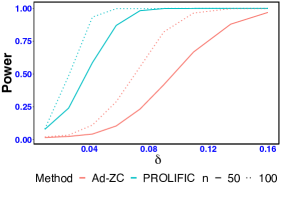
(a) True carryover is non-zero

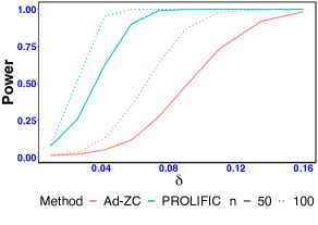
(b) True carryover is zero

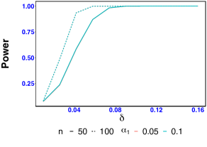
(c) True carryover is non-zero

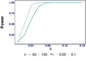
(d) True carryover is zero

Figure 1: Upper panel: Power curve of the PROLIFIC as a function of $\delta$ for $\alpha=0.05$ in comparison to the power of Ad-ZC (when null distribution is approximated by bootstrap) across $n=50$ and $100$, when the true $\lambda(s,d)$ is (a) nonzero and (b) zero, based on $1000$ simulations. The level of the carryover test $\alpha_{1}$ is set at $0.1$. Lower panel: Power curve of PROLIFIC for $\alpha=0.05$ across sample size $n=50$ and $100$ and two different levels of the test of carryover at Stage $1$, $\alpha_{1}=0.05$ and $0.1$, when the true $\lambda(s,d)$ is (c) nonzero and (d) zero.

Size: The empirical type 1 error rate of the PROLIFIC across small ($n=50$) and medium ($n=100$) sample size is presented in Table 2 at specified nominal levels $\alpha=0.01,0.05,0.1$ and $0.15$, with the two different levels ($\alpha_{1}$) of the carryover test at the first stage. The standard error of the estimates are presented in the parenthesis and the numbers are obtained based on $5000$ simulations. Even for sample size as small as $n=50$, the empirical size of PROLIFIC is maintained within twice standard error of the stipulated nominal level. The numbers demonstrate that the size of the overall test is not influenced by the level ($\alpha_{1}$) at which the test of carryover is conducted, as long as both the tests for the significance of the treatment effect at the second stage are conducted at the same level $\alpha$.

Table 3 displays the empirical size of the test conducted by $L_{2}$ norm based statistic of Ad-ZC method, when the null distribution is approximated by mixture of chi-squares. Remarkably, the test fails to maintain the nominal level by large margin, at least for sample size up to $100$. It is possible that a sample of size is $n=100$ is not large enough to fairly approximate the asymptotic null distribution. On the other hand, when the null distribution is approximated by bootstrap, the test exhibits a rather conservative type 1 error.

Power: Fix the level of significance $\alpha=0.05$. The empirical power of PROLIFIC is plotted as a function of $\delta$ for small and medium sample size in Figure 1, based on $1000$ simulations. The left column pertains to the situation when both the carryover and the treatment effect are significant, and the right column when carryover is absent and only the direct treatment effect is significant. We do not present the power of the Ad-ZC when the null distribution is approximated by mixture of chi-squares, because it fails to maintain the size. As expected, in both the cases, we see that the power of the test increases rapidly with the increment in the sample size and as $\delta$ goes away from zero. The upper panel demonstrates that PROLIFIC is more powerful than Ad-ZC to detect departure from null, irrespective whether carryover is zero or not. The overlapping plots in the lower panel illustrate that the power of PROLIFIC is not affected by the level ($\alpha_{1}$) at which the carryover is tested at the first stage.

The strength of PROLIFIC in detecting a very slight departure from null even with very small sample size can be attributed to the fact that both the contrasts for the treatment and the carryover are estimable after removing the variation due to subject and that for every subject, we observe the functional observations over four periods. Overall, the numerical results testify for the effectiveness of the two-stage procedure to detect the significant direct treatment effect in a crossover design, when both the treatment and carryover contrasts are separately estimable, in contrast to the widely criticized lack of power of the two-stage procedure in the case of AB/BA crossover design (Senn, 2002, chapter 3).

5 Meloxicam study of cats with osteoarthritis

The data originates from the meloxicam study of $58$ household cats with existing condition of osteoarthritis. These cats were enrolled in a completely randomized double masked placebo-controlled crossover trial conducted at the College of Veterinary Medicine of North Carolina State University. The subjects were randomized into two groups. As described in Table 1, the first group received the single dose of active drug meloxicam for the 20 days in the first period, followed by placebo during the last three periods. Whereas, group 2 received the drug at period $3$ and received placebo at all the remaining three periods. The objective of study is to understand the efficacy of an active drug meloxicam on the joint pain as reflected by an improved PA counts, measured at every minute level during the day by an activity monitor. See Gruen et al. (2015) for a complete details of the study.

5.1 Data preprocessing

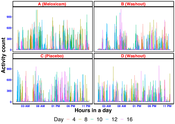
Figure 3: Daily raw activity profiles for a randomly selected cat (cat number $62$) over the days $4,8,10,12$, and $16$ in all the four periods.

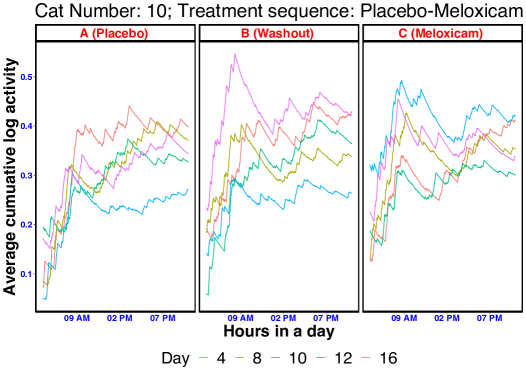
(a)

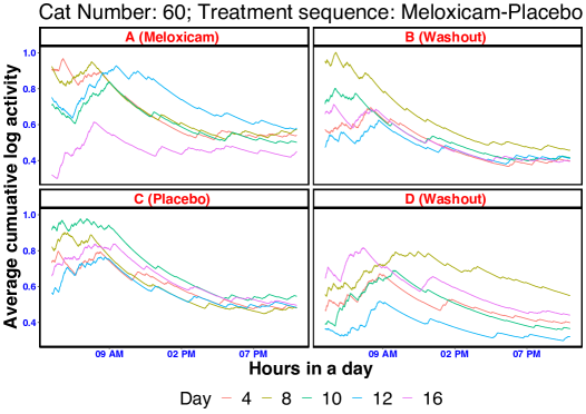
(b)

Figure 4: Cumulative average of the log activity profiles from $5$AM to $10$PM for two randomly selected cats (cat number $10$ and $60$) over the days $4,8,10,12$, and $16$ in all the four periods. No activities were recorded for the cat number $10$ in the last period.

Figure 3(a) presents the daily raw activity counts recorded by Accelerometer for a randomly selected cat over $5$ days in every period. Since the cats in general stays in a resting state for a long period of time, followed by a sudden jump due to some external factors, the raw activity profiles are condensed by a lot of zeros between two high peaks. To reduce the large scale of variation in the activity counts, we add them by $1$ and take the logarithm, i.e. $x\mapsto\log(x+1)$. Let us call these log transformed PA counts as logPA. As a part of the preprocessing step, we take the cumulative average of the logPA at every minute in the day as $Y_{ipj}(s_{r}):=r^{-1}\sum_{\ell=1}^{r}\log(1+\text{PA}_{ipj}(s_{\ell}))$, where $r=1,\dots,1440$ denotes the minutes in a day with $r=1$ referring to the midnight (12:00:00 AM) and $\text{PA}_{ipj}(s_{\ell})$ is the PA counts for the $i$th at the $\ell$th minute of the $j$th day in the $p$th period. We focus on the time of the day from $5$AM to $10$PM, when the owners are more likely to be awake; Figure 4 and 5 show the cumulative average of the logPA for four randomly selected cats during this time over some days in all the four periods. As the profiles are relatively smooth, we work with $Y_{ipj}(s_{r})$ between 5AM to 10PM (i.e. $r=300$ to $1320$) as our response profile.

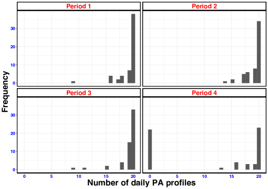
(a) Frequency distribution of $m_{ip}$ across all the periods

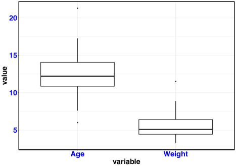
(b) Boxplot of baseline age and weight

Figure 6: (a) Frequency distribution of the number of PA profiles ($m_{ip}$) observed for each of the four periods. (b) Boxplot of the baseline age (in years) and weight (in lbs) of the cats.

There are several baseline covariates collected at the beginning of the study, notable of them are age (in days), weight (WT), a numeric radiologist evaluated disease severity score called as DJD score. The number of PA profiles in each period ($m_{ip}$) varies across the subjects and a frequency distribution of $\left\{m_{ip}\right\}_{i=1}^{n}$ for all the four periods is provided in Figure 6(a). The age of cats in the study varies between 6 years to 21 years with median age of 12 years. Based on a simple boxplot analysis (Figure 6(b)), we removed the cats with $6$ years (cat number 14) and $21$ years (cat number 15) of age from further analysis.

5.2 Data analysis

To test for the significance of the treatment effect, we posit the FACM,

$$Y_{ipj}(s) =\mu(s,\text{Age}_{ipj})+\tau(s,d_{ipj})\;\mathcal{I}_{ip,\tau}+\lambda(s,d_{ipj})\;\mathcal{I}_{ip,\lambda}$$

$$\hskip 108.405pt+\text{WT}_{i}\beta_{1}(s)+\text{WE}_{ipj}\beta_{2}(s)+\text{DJD}_{i}\beta_{3}(s)+\epsilon_{i}(s,d_{ipj}),$$

where $\text{Age}_{ipj}$ is the age of the $i$-th cat at the $j$-th day of the $p$-th period, $\text{WE}_{ipj}$ is the weekend indicator, i.e. it takes values $1$ if the $j$-th day in the $p$-th period is a weekend, otherwise it is zero. All the other components in the model are defined previously. The quantity $\text{Age}_{ipj}$ can be easily computed by adding the baseline age of the cats with the total number days spared in the study period. Instead of including age of the cat at the baseline in an additive manner, we consider that the mean of the response evolves as a smooth function of age, which allows us to the model the effect of age more generally. The DJD score is a factor that is expected to affect the PA. The activities of the cats are also expected to be different over weekdays or weekends, as their owners stay at home and spend more time with them.

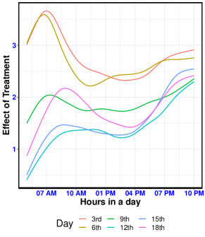
(a) Univariate cross-section of $\widehat{\tau}(\cdot,d)$

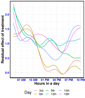
(b) Univariate cross-section of $\widehat{\lambda}(\cdot,d)$

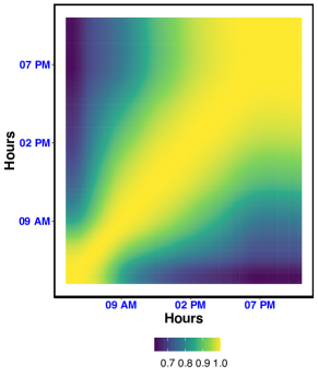
(c) Estimated correlation function

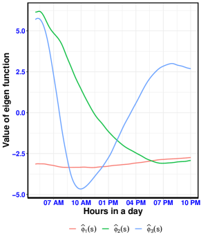
(d) Estimated eigenfunctions, $\widehat{\phi}_{k}(s)$

Figure 2: Upper panel: (a) Estimated treatment $\widehat{\tau}(\cdot,d)$ and (b) carryover $\widehat{\lambda}(\cdot,d)$ for $3$rd, $6$th, $9$th, $12$th, $15$th, and $18$th day in the period. The numbers in the y-axis are multiplied by $100$. Lower panel: (c) Estimated marginal correlation function obtained from $\widehat{\Xi}(s,s^{\prime})$, as a bivariate function of the hours in the day. (d) Estimated eigenfunctions $\widehat{\phi}_{k}(s)$, $k=1,2,3$ as a function of hours in the day, obtained by specifying a PVE $=95\%$.

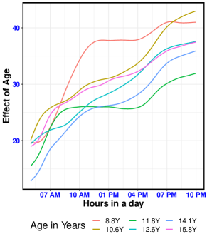
(a) Univariate cross-section of $\widehat{\mu}(s,Age)$

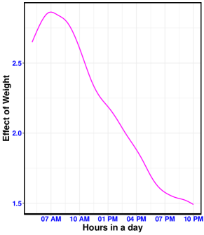
(b) Smooth effect of weight (WT)

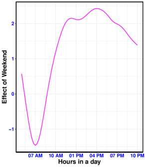
(c) Smooth effect of weekend (WE)

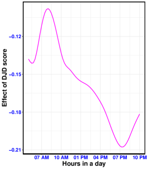
(d) Smooth effect of DJD score

Figure 7: (a) Estimated mean $\widehat{\mu}(\cdot,Age)$ at six equidistant quantiles of the distribution of $Age$ in the data, (b) Estimated effect of weight, $\widehat{\beta}_{1}(s)$ (c) Estimated effect of weekend, $\widehat{\beta}_{2}(s)$ (d) Estimated effect of DJD score, $\widehat{\beta}_{3}(s)$. The numbers in the y-axis are multiplied by $100$.

To test for the significance of the direct treatment effect $H_{0}:\tau(s,d)=0$ vs $H_{1}:\tau(s,d)\neq 0$ for some $s$ and $d$, we implement PROLIFIC as described in Section 3. We estimate the bivariate smooth functions in the model such as $\mu(s,\text{Age}_{ipj})$, and $\tau(s,d_{ipj})$, nonparametrically using a tensor product of cubic spline basis via gam() function in the mgcv package (Wood, 2004) in R. We place the knots at $20$ equidistant points for the dense component $s$ and $5$ equidistant points for the longitudinal component $d$. The smoothing parameters are selected via REML. The upper panel of Figure 2 shows the univariate cross-section of the estimated treatment and the carryover effect over $6$ equidistant days in a period, multiplied by $100$, showing evidence that the effect of treatment is higher in the first half of the period. The estimated effect of all the baseline covariates, multiplied by $100$, are presented in Figure 7. The estimated effect of the DJD score corroborates the negative association of PA with joint pain. A positive association of PA with the weekend can be attributed to the fact that the cats get more time to play with their owners during weekends.

After estimating the fixed components of the model, we demean the response and estimate the marginal covariance function $\widehat{\Xi}(s,s^{\prime})$ via sandwich smoother. The spectral decomposition yields $K=3$ eigenfunctions $\{\widehat{\phi}_{k}(\cdot)\}$ explaining $95\%$ of the total variation. The estimated marginal correlation along with the eigenfunctions are presented in the lower panel of Figure 2. The growing correlation along the center is a direct consequence of the cumulative average of activities, described in the preprocessing step. Using the $\{\widehat{\phi}_{k}(\cdot)\}$, we obtain the projected response $W_{ipj,k}=\sum_{r=1}^{R}Y_{ipj}(s_{r})\widehat{\phi}_{k}(s_{r})$ and consider the projected model

$$W_{ipj,k} =\mu_{k}(\text{Age}_{ipj})+\tau_{k}(d_{ipj})\;\mathcal{I}_{ip,\tau}+\lambda_{k}(d_{ipj})\;\mathcal{I}_{ip,\lambda}$$

$$\hskip 108.405pt+\text{WT}_{i}\beta_{1,k}+\text{WE}_{ipj}\beta_{2,k}+\text{DJD}_{i}\beta_{3,k}+\epsilon_{i,k}(d_{ipj})$$

The framework of PROLIFIC allows us to test for the $H_{0,k}:\tau_{k}(d)=0,\lambda_{k}(d)=0$ vs $H_{1,k}:\tau_{k}(d)\neq 0$, $k=1,2,3$ simultaneously under the projected model. We model the smooth components in the model using a truncated linear basis and apply the two stage testing procedure. For each of $k=1,2,3$, the p-values for the significance test of the carryover effect turn out to be high, suggesting no evidence of the presence of residual effect of the treatment in the washout period. Next we test for the significance of the treatment effect following the test rule in Stage 2b, dropping the carryover term from the projected model. The p-values of the three significance tests for the treatment are $<0.0001$, $0.06$, and $0.11$, suggesting a strong evidence for the significance of the direct effect of meloxicam. The results are coherent with the conclusion based on the p-values $(0.01,0.55,0.41)$ of Ad-ZC test when the null distribution is approximated by $5000$ bootstrap samples. The relatively higher p-values reflect the conservative nature of the Ad-ZC test to detect departure from null, compared to the more powerful PROLIFIC, that we noticed in Section 4.

6 Appendix

The assumptions on which Theorem 3.1 relies are, The number of curves within a period $m_{ip}$ for all $i=1,\dots,n$ and $p=1,\dots,4$ is such that $\sup_{i}\sup_{p}m_{ip}<\infty$. Let $\left\lVert Y\right\rVert:=\underset{s\in\mathcal{S}}{\sup}\left\lvert Y(s)\right\rvert$ for univariate (random) function $Y$ and $\left\lVert Y\right\rVert:=\underset{(s,d)\in\mathcal{S}\times\mathcal{D}}{\sup}\left\lvert Y(s,d)\right\rvert$ for a bivariate (random) function $Y$. Then, $\textrm{E}\left\lVert\epsilon\right\rVert^{2\psi}<\infty$ for some $\psi>1$. The next two assumptions are related to the projected model (5). For $k=1,\dots,K$, The random components ${\bm{\mathbf{{b}}}}_{k}$ and the errors ${\bm{\mathbf{{e}}}}_{k}$ are jointly Gaussian. The minimum eigenvalue of $\bm{\Sigma}_{k}$ is bounded away from zero as $n$ diverges. Let the estimator $\widehat{\bm{\Sigma}}_{W,k}$ of $\bm{\Sigma}_{k}$ satisfies $\mathbf{a}^{\top}\widehat{\bm{\Sigma}}_{W,k}^{-1}\mathbf{a}-\mathbf{a}^{\top}\bm{\Sigma}^{-1}_{k}\mathbf{a}=o_{p}(1)$, and $\mathbf{a}^{\top}\widehat{\bm{\Sigma}}_{W,k}^{-1}{\bm{\mathbf{{e}}}}_{k}-\mathbf{a}^{\top}\bm{\Sigma}^{-1}_{k}{\bm{\mathbf{{e}}}}_{k}=o_{p}(1)$, where $\mathbf{a}$ is any non random $N\times 1$ vector of unit norm. See section S11 of supplementary material for discussion on the assumptions.

S7 Truncated polynomial basis formula for the projected model

Employing the smoothness of $\tau_{k}(d)$, we expand $\tau_{k}(d)$ as a truncated polynomial basis as $\tau_{k}(d)=\alpha_{0\tau,k}+\alpha_{1\tau,k}d+\dots+\alpha_{h_{\tau}\tau,k}d^{h_{\tau}}+\sum_{q=1}^{Q_{\tau}}b_{q\tau,k}(d-\kappa_{q})_{+}^{h_{\tau}}$, where $\kappa_{1},\dots,\kappa_{Q_{\tau}}$ are appropriately placed knots (Ruppert et al., 2003). Similarly, we can expand the other smooth effects $\mu_{k}(d)$ and $\lambda_{k}(d)$ as $\mu_{k}(d)=\alpha_{0\mu,k}+\alpha_{1\mu,k}d+\dots+\alpha_{h_{\mu}\mu,k}d^{h_{\mu}}+\sum_{q=1}^{Q_{\mu}}b_{q\mu,k}(d-\kappa_{q})_{+}^{h_{\mu}}$ and $\lambda_{k}(d)=\alpha_{0\lambda,k}+\alpha_{1\lambda,k}d+\dots+\alpha_{h_{\lambda}\lambda,k}d^{h_{\lambda}}+\sum_{q=1}^{Q_{\lambda}}b_{q\lambda,k}(d-\kappa_{q})_{+}^{h_{\lambda}}$. Denote by ${\bm{\mathbf{{\alpha}}}}_{\mu,k}=\left(\alpha_{0\mu,k},\alpha_{1\mu,k},\dots,\alpha_{h_{\mu}\mu,k}\right)^{\top}$ the vector of the coefficients corresponding to the polynomial basis and by ${\bm{\mathbf{{b}}}}_{\mu,k}=\left(b_{1\mu,k},\dots,b_{Q_{\mu}\mu,k}\right)^{\top}$ the vector of spline coefficients for the mixed model representation of the smooth mean $\mu_{k}(d)$. Similarly, denote by ${\bm{\mathbf{{\alpha}}}}_{\tau,k}=\left(\alpha_{0\tau,k},\alpha_{1\tau,k},\dots,\alpha_{h_{\tau}\tau,k}\right)^{\top}$ the vector of the coefficients corresponding to the polynomial basis and by ${\bm{\mathbf{{b}}}}_{\tau,k}=\left(b_{1\tau,k},\dots,b_{Q_{\tau}\tau,k}\right)^{\top}$ the vector of spline coefficients for the smooth treatment effect $\tau_{k}(d)$; and ${\bm{\mathbf{{\alpha}}}}_{\lambda,k}$, ${\bm{\mathbf{{b}}}}_{\lambda,k}$ as the vector of polynomial basis coefficients and the spline coefficients respectively for the carryover effect $\lambda_{k}(d)$. As it is common in the literature we treat the coefficients of the polynomial terms as fixed but unknown parameters and the coefficients of the non-polynomial terms as random. Using the mixed model representation we can write $\mu_{k}(d_{ipj})=\mathbf{X}^{\top}_{ipj,\mu}\bm{\alpha}_{\mu,k}+\mathbf{Z}^{\top}_{ipj,\mu}\mathbf{b}_{\mu,k}$, where $\mathbf{X}^{\top}_{ipj,\mu}=(1,d_{ipj},\ldots,d_{ipj}^{h_{\mu}})$, $\mathbf{Z}^{\top}_{ipj,\tau}=((d_{ipj}-\kappa_{1})_{+}^{h_{\mu}},\ldots,(d_{ipj}-\kappa_{Q_{\mu}})_{+}^{h_{\mu}})$ and $b_{q\mu,k}$’s, are assumed to be iid with mean zero and variance $\sigma^{2}_{\mu,k}$ for $q=1,\ldots,{Q_{\mu}}$. For the treatment effect we can similarly write, $\tau_{k}(d_{ipj})\mathcal{I}_{ip,\tau}=\mathbf{X}^{\top}_{ipj,\tau}\bm{\alpha}_{\tau,k}+\mathbf{Z}^{\top}_{ipj,\tau}\mathbf{b}_{\tau,k}$, where $\mathbf{X}^{\top}_{ipj,\tau}=\mathcal{I}_{ip,\tau}\cdot(1,d_{ipj},\ldots,d_{ipj}^{h_{\tau}})$, $\mathbf{Z}^{\top}_{ipj,\tau}=\mathcal{I}_{ip,\tau}\cdot((d_{ipj}-\kappa_{1})_{+}^{h_{\tau}},\ldots,(d_{ipj}-\kappa_{Q_{\tau}})_{+}^{h_{\tau}})$ and $b_{q\tau,k}\overset{iid}{\sim}(0,\sigma^{2}_{\tau,k})$’s, and $\lambda_{k}(d_{ipj})\mathcal{I}_{ip,\lambda}$ as $\mathbf{X}^{\top}_{ipj,\lambda}\bm{\alpha}_{\lambda,k}+\mathbf{Z}^{\top}_{ipj,\lambda}\mathbf{b}_{\lambda,k}$ with $b_{q\lambda,k}\overset{iid}{\sim}(0,\sigma^{2}_{\lambda,k})$.

Let ${\bm{\mathbf{{X}}}}_{i,\mu}$ be the ${m_{i\centerdot}\times({h_{\mu}}+1)}$ fixed design matrix constructed by row-stacking $\mathbf{X}^{\top}_{ipj,\mu}$ over $p$ and $j$ and ${\bm{\mathbf{{Z}}}}_{i,\mu}$ be the ${m_{i\centerdot}\times{Q_{\mu}}}$ random design matrix obtained by row-stacking ${\bm{\mathbf{{Z}}}}^{\top}_{ipj,\mu}$, where $m_{i\centerdot}:=\sum_{p=1}^{4}m_{ip}$. Similarly, construct ${\bm{\mathbf{{X}}}}_{i,\tau}$ and ${\bm{\mathbf{{Z}}}}_{i,\tau}$ for the treatment effect and ${\bm{\mathbf{{X}}}}_{i,\lambda}$ and ${\bm{\mathbf{{Z}}}}_{i,\lambda}$ for the carryover effect respectively. Further construct a $m_{i\centerdot}\times L$ matrix $\mathbf{X}_{i,w}$ corresponding to the baseline covariates $C_{i\ell}$ in the model (4), i.e. $\mathbf{X}_{i,w}={\bm{\mathbf{{1}}}}_{m_{i\centerdot}}\otimes\left[C_{i1},\dots,C_{iL}\right]$ and column stack it with ${\bm{\mathbf{{X}}}}_{i,\mu}$ to construct ${\bm{\mathbf{{X}}}}_{i,b}=[{\bm{\mathbf{{X}}}}_{i,\mu},{\bm{\mathbf{{X}}}}_{i,w}]$, where ${\bm{\mathbf{{1}}}}_{m_{i\centerdot}}$ is the $m_{i\centerdot}$-length column vector $1$’s and $\otimes$ denotes the Kronecker product. Denote by $N:=\sum_{i=1}^{n}m_{i\centerdot}$ the total number of curves for all the subjects, by ${\bm{\mathbf{{X}}}}_{b}=\left[{\bm{\mathbf{{X}}}}_{1,b}^{\top},\dots,{\bm{\mathbf{{X}}}}_{n,b}^{\top}\right]^{\top}$ the $N\times(L+h_{\mu}+1)$ matrix of ${\bm{\mathbf{{X}}}}_{i,b}$’s, by ${\bm{\mathbf{{X}}}}_{\tau}=\left[{\bm{\mathbf{{X}}}}_{1,\tau}^{\top},\dots,{\bm{\mathbf{{X}}}}_{n,\tau}^{\top}\right]^{\top}$ the $N\times({h_{\tau}}+1)$ matrix of fixed effect for $\tau_{k}(d)$, by ${\bm{\mathbf{{X}}}}_{\lambda}=\left[{\bm{\mathbf{{X}}}}_{1,\lambda}^{\top},\dots,{\bm{\mathbf{{X}}}}_{n,\lambda}^{\top}\right]^{\top}$ the $N\times({h_{\lambda}}+1)$ matrix of fixed effect for $\lambda_{k}(d)$, by ${\bm{\mathbf{{Z}}}}_{\tau}=\left[{\bm{\mathbf{{Z}}}}_{1,\tau}^{\top},\dots,{\bm{\mathbf{{Z}}}}_{n,\tau}^{\top}\right]^{\top}$ the $N\times{Q_{\tau}}$ matrix of ${\bm{\mathbf{{Z}}}}_{i,\tau}$’s and by ${\bm{\mathbf{{Z}}}}_{\lambda}=\left[{\bm{\mathbf{{Z}}}}_{1,\lambda}^{\top},\dots,{\bm{\mathbf{{Z}}}}_{n,\lambda}^{\top}\right]^{\top}$ the $N\times{Q_{\lambda}}$ matrix of ${\bm{\mathbf{{Z}}}}_{i,\lambda}$’s. Furthermore, let $\mathbf{Y}_{k}=\left[{\bm{\mathbf{{Y}}}}_{1,k}^{\top},\dots,{\bm{\mathbf{{Y}}}}_{n,k}^{\top}\right]^{\top}$ with ${\bm{\mathbf{{Y}}}}_{i,k}$ be the columns vector of the projected responses for $i$th subject by stacking $Y_{ipj,k}$ over $p$ and $j$’s, and the residual vector ${\bm{\mathbf{{e}}}}_{k}=\left[{\bm{\mathbf{{e}}}}_{1,k}^{\top},\dots,{\bm{\mathbf{{e}}}}_{n,k}^{\top}\right]^{\top}$ with ${\bm{\mathbf{{e}}}}_{i,k}$ is constructed by stacking $\epsilon_{i,k}(d_{ipj})$ over all $p$ and $j$.

S8 Selection of the orthogonal basis

Testing the original hypothesis problem in (2) reduces to simultaneous sequential testing of $H_{01,k}$ and $H_{02,k},k=1,\dots,K$ for a large value of $K$. Moreover, the above testing framework requires a specified set of orthogonal basis system $\left\{\phi_{k}(s)\right\}_{k\geq 1}$ for the space $\mathcal{L}^{2}(\mathcal{S})$ to compute the projected response and test $H_{0k}$ under the projected model (4). Theoretically, any known preset orthogonal basis function such Fourier basis, wavelets or Legendre basis will work. However the selection of truncation parameter $K$ becomes difficult, and typically that will require to test a very large number of simpler hypotheses of the form $H_{0,k}$. To avoid this, we choose a set of data-driven eigenbases from an appropriate covariance function, as adopted by Koner et al. (2021). Specifically, define the so-called “marginal covariance” $\Xi(s,s^{\prime})$ of the error process $\epsilon_{i}(s,d_{ipj})$ in model (1) by marginalizing over the the sampling distribution of the design points $d_{ipj}$’s. As $\Xi(s,s^{\prime})$ is guaranteed to be a proper covariance function (Park and Staicu, 2015), we extract the eigenfunctions $\left\{\phi_{k}(s)\right\}$ from the spectral decomposition of $\Xi(s,s^{\prime})$ (Mercer, 1909). Finally, the truncation parameter $K$ is chosen as the minimum value of $K$ such that $\sum_{k=1}^{K}\lambda_{k}/\operatorname{tr}(\Xi)\geq\text{PVE}$, where $\lambda_{1}\geq\lambda_{2}\geq\dots\geq 0$ are the eigenvalues, $\operatorname{tr}(\Xi):=\int\Xi(s,s)ds$ is the trace of the covariance $\Xi(s,s^{\prime})$ and the PVE (typically $95\%$) is some pre-specified threshold indicating the percentage of variation explained.

Although using a set of eigenfunctions identifies principal sources of variations in the data and provides an objective framework for choosing $K$ parsimoniously, in practice these eigenfunctions are unknown. As a result, the projected response $Y_{ipj,k}$ can not be computed unless the eigenfunction are estimated with high accuracy. A detailed description of the estimation of the eigenfunctions from the marginal covariance is laid out in Koner et al. (2021), we omit it here to avoid redundancy. We develop the testing procedure using these estimated set of eigenfunctions $\left\{\widehat{\phi}_{k}(\cdot):k=1,\ldots,K\right\}$ as our choice of orthogonal basis functions. Furthermore, we derive the null distribution of the proposed test statistic; the results rely on the uniform convergence of the eigenfunctions estimators (Theorem 3.1).

S9 Additional results related to PROLIFIC

Corollary S9.1

Assume all the conditions of the Theorem 3.1. Let $\left\{\xi_{\tau,k,s}(\pi_{k},\gamma_{k})\right\}_{s=1}^{Q_{\tau}}$ be the eigenvalues of the $Q_{\tau}\times Q_{\tau}$ matrix $\widetilde{\mathbf{Z}}_{\tau,k}^{\top}\widetilde{\mathbf{V}}_{k}(\pi_{k},0,\gamma_{k})^{-1}(\mathbf{I}_{N}-\widetilde{\mathbf{H}}_{k}(\pi_{k},0,\gamma_{k}))\widetilde{\mathbf{Z}}_{\tau,k}$. Then under the null hypothesis in (2) the test statistic has an approximate distribution as follows

$$pqGF_{N,k}^{S2a}\overset{d}{\approx}\frac{\sum_{s=1}^{Q_{\tau}}\frac{\widehat{\eta}_{k}\xi_{\tau,k,s}(\widehat{\pi}_{k},\widehat{\gamma}_{k})}{1+\widehat{\eta}_{k}\xi_{\tau,k,s}(\widehat{\pi}_{k},\widehat{\gamma}_{k})}u_{s}^{2}+\chi^{2}_{h_{\tau}+1}+o_{p}(1)}{\frac{1}{N}\left\{\sum_{s=1}^{Q_{\tau}}\frac{1}{1+\widehat{\eta}_{k}\xi_{\tau,k,s}(\widehat{\pi}_{k},\widehat{\gamma}_{k})}u_{s}^{2}+\chi^{2}_{N-r-Q_{\tau}}\right\}+o_{p}(1)},$$ (14)

where $u_{s}\overset{iid}{\sim}\textrm{N}(0,1)$ and independent with $\chi^{2}_{h_{\tau}+1}$ and $\chi^{2}_{N-r-Q_{\tau}}$, and

$$(\widehat{\pi}_{k},\widehat{\eta}_{k},\widehat{\gamma}_{k}):= \operatorname*{arg\,min}_{\pi_{k},\eta_{k},\gamma_{k}}\;\;\left[(N-r)\log\left\{\sum_{s=1}^{Q_{\tau}}\frac{u_{s}^{2}}{1+\eta_{k}\xi_{\tau,k,s}(\pi_{k},\gamma_{k})}+\chi^{2}_{N-r-Q_{\tau}}\right\}\right.$$

$$\hskip 72.26999pt+\left.\sum_{s=1}^{Q_{\tau}}\log\left\{1+\eta_{k}\xi_{\tau,k,s}(\pi_{k},\gamma_{k})\right\}+\sum_{s=1}^{Q_{\mu}+Q_{\lambda}}\log\left\{1+\omega_{-\tau,k,s}(\pi_{k},\gamma_{k})\right\}\right],$$

where $\omega_{-\tau,k,s}(\pi_{k},\gamma_{k})$ be the $s$th eigenvalue of the $(Q_{\mu}+Q_{\lambda})\times(Q_{\mu}+Q_{\lambda})$ matrix $\mathbf{D}_{-\tau}(\pi_{k},\gamma_{k})\widetilde{\mathbf{Z}}_{-\tau,k}^{\top}(\mathbf{I}_{N}-\widetilde{\mathbf{P}}_{k})\widetilde{\mathbf{Z}}_{-\tau,k}\mathbf{D}_{-\tau}(\pi_{k},\gamma_{k})$ with $\mathbf{D}_{-\tau}(\pi_{k},\gamma_{k}):=\mathrm{diag}(\sqrt{\pi_{k}}\;\mathbf{I}_{Q_{\mu}},\sqrt{\gamma_{k}}\;\mathbf{I}_{Q_{\lambda}})$.

Corollary S9.2

Assume that all the conditions of the Theorem 3.1 hold. Suppose, $\xi_{\tau,k,s}(\pi_{k})$ be the $s$th eigenvalue of the $Q_{\tau}\times Q_{\tau}$ matrix $\widetilde{\mathbf{Z}}_{\tau,k}^{\top}\widetilde{\mathbf{V}}_{k}(\pi_{k},0,0)^{-1}(\mathbf{I}_{N}-\widetilde{\mathbf{H}}_{-\lambda,k}^{S2b})\widetilde{\mathbf{Z}}_{\tau,k}$ with $\widetilde{\mathbf{H}}_{-\lambda,k}^{S2b}:=\widetilde{\mathbf{X}}_{-\lambda,k}\left(\widetilde{\mathbf{X}}_{-\lambda,k}^{\top}\widetilde{\mathbf{V}}_{k}(\pi_{k},0,0)^{-1}\widetilde{\mathbf{X}}_{-\lambda,k}\right)^{-1}\widetilde{\mathbf{X}}_{-\lambda,k}^{\top}\widetilde{\mathbf{V}}_{k}(\pi_{k},0,0)^{-1}$ is the generalized projection onto column space of $\widetilde{\mathbf{X}}_{-\lambda,k}$. Under the null hypothesis in (2) the test statistic has an approximate distribution,

$${pqGF}_{N,k}^{S2b}\overset{d}{\approx}\frac{\sum_{s=1}^{Q_{\tau}}\frac{\widehat{\eta}_{k}\xi_{\tau,k,s}(\widehat{\pi}_{k})}{1+\widehat{\eta}_{k}\xi_{\tau,k,s}(\widehat{\pi}_{k})}u_{s}^{2}+\chi^{2}_{h_{\tau}+1}+o_{p}(1)}{\frac{1}{N}\left\{\sum_{s=1}^{Q_{\tau}}\frac{1}{1+\widehat{\eta}_{k}\xi_{\tau,k,s}(\widehat{\pi}_{k})}u_{s}^{2}+\chi^{2}_{N-r_{0}-Q_{\tau}}\right\}+o_{p}(1)},$$ (15)

where $r_{0}:=L+h_{\mu}+h_{\tau}+2$ is the rank of $\widetilde{\mathbf{X}}_{-\lambda,k}$ , $u_{s}\overset{iid}{\sim}\textrm{N}(0,1)$ and independent with $\chi^{2}_{h_{\tau}+1}$ and $\chi^{2}_{N-r_{0}-Q_{\tau}}$ and

$$(\widehat{\pi}_{k},\widehat{\eta}_{k}):= \operatorname*{arg\,min}_{\pi_{k},\eta_{k}}\;\;\left[(N-r_{0})\log\left\{\sum_{s=1}^{Q_{\tau}}\frac{u_{s}^{2}}{1+\eta_{k}\xi_{\tau,s,k}(\pi_{k})}+\chi^{2}_{N-r_{0}-Q_{\tau}}\right\}\right.$$

$$\hskip 108.405pt+\left.\sum_{s=1}^{Q_{\tau}}\log\left\{1+\eta_{k}\xi_{\tau,s,k}(\pi_{k})\right\}+\sum_{s=1}^{Q_{\mu}}\log\left\{1+\pi_{k}\omega_{s,k}\right\}\right],$$

where $\omega_{s,k}$ be the $s$th eigenvalue of the $Q_{\mu}\times Q_{\mu}$ matrix $\widetilde{\mathbf{Z}}_{\mu,k}^{\top}(\mathbf{I}_{N}-\widetilde{\mathbf{P}}_{-\lambda,k})\widetilde{\mathbf{Z}}_{\mu,k}$ with $\widetilde{\mathbf{P}}_{-\lambda,k}:=\widetilde{\mathbf{X}}_{-\lambda,k}(\widetilde{\mathbf{X}}_{-\lambda,k}^{\top}\widetilde{\mathbf{X}}_{-\lambda,k})^{-1}\widetilde{\mathbf{X}}_{-\lambda,k}^{\top}$.

S10 Details of estimation of FACM

To obtain the smooth estimates of bivariate mean function $\widehat{\mu}(s,d)$, treatment effect $\widehat{\tau}(s,d)$ and carryover effect $\widehat{\lambda}(s,d)$ we fit the FACM using gam() function in R package mgcv (Wood, 2004). Using the residulals, we estimate the marginal covariance using the bivariate sandwich smoother by Xiao et al. (2013) implemented in the fpca.face() in R package refund (Goldsmith et al., 2020). After estimating $K$ and the eigenfunctions $\widehat{\phi}_{k}(s)$ with a PVE of $90\%$, we project the response onto the direction of the eigenfunctions. Next, we fit the smooth components of the projected model (4) using a truncated linear basis $(h_{\mu}=h_{\tau}=h_{\lambda}=1)$ by placing the knots $\kappa_{1},\dots,\kappa_{Q}$ at a equally spaced quantile levels of the observed visit times $\left\{\left\{d_{ipj}\right\}_{j=1}^{m_{ip}}:i,p\right\}$ with a number of knots $Q=\max\{20,\min(0.25\times\text{ number of unique }d_{ipj},40)\}$ (Ruppert et al., 2003), which is also the same for $\mu,\tau$ and $\lambda$. For each $k$, the covariance function $\bm{\Sigma}_{k}$ of $\epsilon_{i,k}(d_{ipj})$ is estimated nonparametrically using fpca.sc() function in refund package. The number of eigenfunction is chosen with PVE of $90\%$. After denoising the quasi projections $W_{k,ij}$ with the inverse square root of estimated covariance matrix $\widehat{\bm{\Sigma}}_{W,k}$, we fit the LMM in (5) using the lme() function in nlme (Pinheiro et al., 2021) package and conduct the two-stage test in (12) by simulating from null distribution of the test statistics in (7), (14) and (15) implementing algorithm B of Wang and Chen (2012). Finally the overall conclusion for the hypothesis (2) is drawn combining the results of each of the $k=1,\dots,K$ tests as per the rule (13).

S11 Discussion of assumptions

Assumption 6 ensures that the number of curves for all subjects are finite. The moment condition in Assumption 6 is very common in FDA literature (Zhang et al., 2016; Xiao et al., 2020). It relates to the continuity of the sample paths of the error process $\epsilon(s,d)$. The condition ensures that the projection of the response trajectory onto the eigenfunction $\phi_{k}(\cdot)$, $Y_{ipj,k}=\int Y_{ipj}(s)\phi_{k}(s)ds$ is consistently defined and that the projected response has finite second moment. Assumption 6 states that the unobserved projected response $\mathbf{Y}_{k}$ in model (5) is multivariate Gaussian and is the key ingredient to derive the null distribution of the test statistic in Theorem 3.1. Gaussianity of $Y_{ipj,k}$ follows if the original response $Y_{ipj}(\cdot)$ is distributed as a Gaussian process with continuous sample paths and the eigenfunctions $\left\{\phi_{k}(\cdot)\right\}_{k\geq 1}$ are continuous (Taylor and Karlin, 2014, chapter 8). We want to point out that we do not make any distributional assumption for the quasi-projections $W_{ipj,k}$, which are based on the eigenfunctions $\widehat{\phi}_{k}(\cdot)$ that are estimated from the full data. Assumption 6, inspired by Staicu et al. (2014), is crucial to justify that the approximation error by pre-whitening the response with the estimator of the true covariance function $\bm{\Sigma}_{k}$ goes away as $n\to\infty$. When the eigenfunctions $\left\{\phi_{k}(\cdot)\right\}_{k\geq 1}$ are estimated consistently at a certain uniform rate of convergence, the accuracy in the estimation of $\bm{\Sigma}_{k}$ through the quasi projections $W_{ipj,k}$ does not degrade compared to when $\bm{\Sigma}_{k}$ is estimated through the unobserved projected response $Y_{ipj,k}$. A mathematical justification of this is provided in the appendix of Koner et al. (2021).

S12 Proof of theorems and corollaries

The proof of Corollary S9.1 and S9.2 goes exactly in the same way as the proof of Theorem 3.1. We provide a detailed proof of the Theorem 3.1 and omit the proofs of the corollaries to avoid redundancy.

We first derive the asymptotic null distribution of ${pqGF}_{N,k}^{S1}$, assuming that $\pi_{k}$ and $\eta_{k}$ are known. The linear mixed effect model in (5) can be equivalently written as

$$\mathbf{Y}_{k}=\mathbf{X}_{-\lambda,k}\bm{\alpha}_{-\lambda,k}+\mathbf{X}_{\lambda,k}\bm{\alpha}_{\lambda,k}+\mathbf{Z}_{\lambda,k}\mathbf{b}_{\lambda,k}+\mathbf{E}_{k},$$

where $\bm{\alpha}_{-\lambda,k}:=(\bm{\alpha}_{b,k}^{\top},\bm{\alpha}_{\tau,k}^{\top})^{\top}$ and under assumption 6, $\mathbf{E}_{k}$ follows a Normal distribution with variance $\sigma^{2}_{k}\left(\bm{\Sigma}_{k}+\pi_{k}\mathbf{Z}_{\mu}\mathbf{Z}_{\mu}^{\top}+\eta_{k}\mathbf{Z}_{\tau}\mathbf{Z}_{\tau}^{\top}\right)$. Now, define, $\mathbf{V}_{0,k}:=\mathbf{I}_{N}+\pi_{k}\bm{\Sigma}_{k}^{-1/2}\mathbf{Z}_{\mu}\mathbf{Z}_{\mu}^{\top}\bm{\Sigma}_{k}^{-1/2\top}+\eta_{k}\bm{\Sigma}_{k}^{-1/2}\mathbf{Z}_{\tau}\mathbf{Z}_{\tau}^{\top}\bm{\Sigma}_{k}^{-1/2\top}$. Denote the scaled version data and the design matrices of the model by the inverse square root of the true covariance of the data under the null model as $\mathbf{Y}_{k}^{0}:=\mathbf{V}_{0,k}^{-1/2}\bm{\Sigma}^{-1/2}_{k}\mathbf{Y}_{k}$, $\mathbf{X}_{k}^{0}:=\mathbf{V}_{0,k}^{-1/2}\bm{\Sigma}^{-1/2}_{k}\mathbf{X}=[\mathbf{X}_{-\lambda,k}^{0},\mathbf{X}_{\lambda,k}^{0}]$, $\mathbf{Z}_{-\lambda,k}^{0}:=\mathbf{V}_{0,k}^{-1/2}\bm{\Sigma}^{-1/2}_{k}\mathbf{Z}_{-\lambda,k}$ and $\mathbf{E}_{k}^{0}:=\mathbf{V}_{0,k}^{-1/2}\bm{\Sigma}^{-1/2}_{k}\mathbf{E}_{k}$. Then the linear mixed effect model can be conveniently written as

$$\mathbf{Y}_{k}^{0}=\mathbf{X}^{0}_{-\lambda,k}\bm{\alpha}_{-\lambda,k}+\mathbf{X}^{0}_{\lambda,k}\bm{\alpha}_{\lambda,k}+\mathbf{Z}^{0}_{\lambda,k}\mathbf{b}_{\lambda,k}+\mathbf{E}^{0}_{k},$$

where $\mathbf{E}^{0}_{k}\sim N(0,\sigma^{2}_{k}\mathbf{I}_{N})$. Define $N\times r$ matrix $\mathbf{G}_{k}^{0}$ and $N\times(h_{\lambda}+1)$ matrix $\mathbf{G}_{\lambda,k}^{0}$, both with orthonormal columns, such that $\mathbf{G}_{k}^{0}\mathbf{G}_{k}^{0\top}=\mathbf{I}_{N}-\mathbf{X}_{k}^{0}(\mathbf{X}_{k}^{0\top}\mathbf{X}_{k}^{0})^{-1}\mathbf{X}_{k}^{0\top}$ and $\mathbf{G}_{\lambda,k}^{0}\mathbf{G}_{\lambda,k}^{0\top}=\mathbf{X}_{k}^{0}(\mathbf{X}_{k}^{0\top}\mathbf{X}_{k}^{0})^{-1}\mathbf{X}_{k}^{0\top}-\mathbf{X}_{-\lambda,k}^{0}(\mathbf{X}_{-\lambda,k}^{0\top}\mathbf{X}_{-\lambda,k}^{0})^{-1}\mathbf{X}_{-\lambda,k}^{0\top}$.

For notational simplicity, denote the covariance matrix in the statement of the theorem, $\widetilde{\mathbf{V}}_{k}(\pi_{k},\eta_{k},0)$ as $\widetilde{\mathbf{V}}_{0,k}$. Further define, $\widetilde{\mathbf{W}}_{0,k}=\widetilde{\mathbf{V}}_{0,k}^{-1/2}\widetilde{\mathbf{W}}_{k}$, $\widetilde{\mathbf{Y}}_{0,k}=\widetilde{\mathbf{V}}_{0,k}^{-1/2}\widehat{\bm{\Sigma}}_{W,k}^{-1/2}\mathbf{Y}_{k}$, $\widetilde{\mathbf{X}}_{0,k}=\widetilde{\mathbf{V}}_{0,k}^{-1/2}\widetilde{\mathbf{X}}_{k}$, $\widetilde{\mathbf{Z}}_{0,k}=\widetilde{\mathbf{V}}_{0,k}^{-1/2}\widetilde{\mathbf{Z}}_{k}$ and $\widetilde{\mathbf{E}}_{0,k}=\widetilde{\mathbf{V}}_{0,k}^{-1/2}\widehat{\bm{\Sigma}}_{W,k}^{-1/2}\mathbf{E}_{k}$. Call $\widetilde{\mathbf{V}}_{1,k}:=\mathbf{I}_{N}+\widehat{\gamma}_{k}\widetilde{\mathbf{Z}}_{\lambda,0,k}\widetilde{\mathbf{Z}}_{\lambda,0,k}^{\top}=\widetilde{\mathbf{V}}_{0,k}^{-1/2}\widetilde{\mathbf{V}}_{k}\widetilde{\mathbf{V}}_{0,k}^{-1/2}$. Further, define $\widetilde{\mathbf{P}}_{0,k}:=\widetilde{\mathbf{X}}_{0,k}(\widetilde{\mathbf{X}}_{0,k}^{\top}\widetilde{\mathbf{X}}_{0,k})^{-1}\widetilde{\mathbf{X}}_{0,k}^{\top}$ be the projection matrix onto the column space of $\widetilde{\mathbf{X}}_{0,k}$. Further define, $\widetilde{\mathbf{P}}_{-\lambda,0,k}:=\widetilde{\mathbf{X}}_{-\lambda,0,k}(\widetilde{\mathbf{X}}_{-\lambda,0,k}^{\top}\widetilde{\mathbf{X}}_{-\lambda,0,k})^{-1}\widetilde{\mathbf{X}}_{-\lambda,0,k}^{\top}$ be the projection matrix onto the column space of $\widetilde{\mathbf{X}}_{-\lambda,0,k}$, where $\widetilde{\mathbf{X}}_{-\lambda,0,k}$ is the submatrix of $\widetilde{\mathbf{X}}_{0,k}$ after removing the columns corresponding to $\bm{\alpha}_{\lambda,k}$. Since $\mathbf{I}_{N}-\widetilde{\mathbf{P}}_{0,k}$ is a projection matrix with rank $N-r$, there exists a $N\times(N-r)$ matrix $\widetilde{\mathbf{G}}_{0,k}$ with orthonormal columns such that,

$$\widetilde{\mathbf{G}}_{0,k}\widetilde{\mathbf{G}}_{0,k}^{\top} =\mathbf{I}_{N}-\widetilde{\mathbf{P}}_{0,k},\quad\widetilde{\mathbf{G}}_{0,k}^{\top}\widetilde{\mathbf{G}}_{0,k}=\mathbf{I}_{N-r}.$$

$$\widetilde{\mathbf{G}}_{0,k}^{\top}\widetilde{\mathbf{V}}_{1,k}\widetilde{\mathbf{G}}_{0,k} =\widetilde{\mathbf{G}}_{0,k}^{\top}\left(\mathbf{I}_{N}+\widehat{\gamma}_{k}\widetilde{\mathbf{Z}}_{\lambda,0,k}\widetilde{\mathbf{Z}}_{\lambda,0,k}^{\top}\right)\widetilde{\mathbf{G}}_{0,k}=\mathbf{I}_{N-r}+\widehat{\gamma}_{k}\widetilde{\mathbf{D}}_{k},$$ (16)

where $\widetilde{\mathbf{D}}_{k}:=\textrm{diag}(\widetilde{\zeta}_{1,k},\dots,\widetilde{\zeta}_{N-r,k})$ with $\widetilde{\zeta}_{s}$ being the $s$th eigenvalue of the $(N-r)\times(N-r)$ matrix $\widetilde{\mathbf{G}}_{0,k}^{\top}\widetilde{\mathbf{Z}}_{\lambda,0,k}\widetilde{\mathbf{Z}}_{\lambda,0,k}^{\top}\widetilde{\mathbf{G}}_{0,k}$. See the supplementary material of Wang and Chen (2012) for the construction of this matrix $\widetilde{\mathbf{G}}_{0,k}$. Moreover, since $\widetilde{\mathbf{P}}_{0,k}-\widetilde{\mathbf{P}}_{-\lambda,0,k}$ is also a projection matrix with rank $(h_{\lambda}+1)$, there exists a $N\times(h_{\lambda}+1)$ matrix with orthonormal columns $\widetilde{\mathbf{G}}_{\lambda,0,k}$ such that $\widetilde{\mathbf{G}}_{\lambda,0,k}\widetilde{\mathbf{G}}_{\lambda,0,k}^{\top}=\widetilde{\mathbf{P}}_{0,k}-\widetilde{\mathbf{P}}_{-\lambda,0,k}$.

The most fascinating thing in the proof is that even after using the quasi-projection $W_{ipj,k}$ instead of the unobserved projection $Y_{ipj,k}$ we get null distribution that is same to what Oh et al. (2019) obtained using a known eigenfunction, upto a a remainder term that sharply goes to zero in probability at a rate that is dependent on the convergence rate of the eigenfunctions $\widehat{\phi}_{k}(s)$ and accuracy rate of estimation of $\bm{\Sigma}_{k}$. By the definition of $W_{ipj,k}$ and $Y_{ipj,k}$, the difference between these two quantities are,

$$\delta_{ipj,k} :=W_{ipj,k}-Y_{ipj,k}=\int_{\mathcal{S}}Y_{ipj}(s)\left(\widehat{\phi}_{k}(s)-\phi_{k}(s)\right)ds$$ (17)

$$=\int_{\mathcal{S}}\textrm{E}(Y_{ipj}(s))\left(\widehat{\phi}_{k}(s)-\phi_{k}(s)\right)ds+\int_{\mathcal{S}}\epsilon_{i}(s,d_{ipj})\left(\widehat{\phi}_{k}(s)-\phi_{k}(s)\right)ds$$

$$=\underline{\delta}_{ipj,k}+\bar{\delta}_{ipj,k}.$$ (18)

Note that under the null, $\underline{\delta}_{ipj,k}:=\int_{\mathcal{S}}\{\mu(s,d_{ipj})+\tau(s,d_{ipj})\;\mathcal{I}_{ip,\tau}+\sum_{l=1}^{L}W_{il}\beta_{l}(s)\}(\widehat{\phi}_{k}(s)-\phi_{k}(s))ds$. Define, $\bm{\delta}_{i,k}:=(\bm{\delta}_{i1,k}^{\top},\dots,\bm{\delta}_{i4,k}^{\top})^{\top}$; $\bm{\delta}_{ip,k}:=(\delta_{ip1,k},\dots,\delta_{ipm_{ip},k})^{\top}$. Define, $\bm{\delta}_{k}:=(\bm{\delta}_{1,k}^{\top},\dots,\bm{\delta}_{n,k}^{\top})^{\top}$ are stacked version of $\bm{\delta}_{i,k}$’s for all subjects. Similarly define $\underline{\bm{\delta}}_{k}:=(\underline{\bm{\delta}}_{1,k}^{\top},\dots,\underline{\bm{\delta}}_{n,k}^{\top})^{\top}$ and $\bar{\bm{\delta}}_{k}:=(\bar{\bm{\delta}}_{1,k}^{\top},\dots,\bar{\bm{\delta}}_{n,k}^{\top})^{\top}$. Further define the scaled version of these as $\widetilde{\bm{\delta}}_{0,k}:=\widetilde{\mathbf{V}}_{0,k}^{-1/2}\widehat{\bm{\Sigma}}^{-1/2}_{W,k}\bm{\delta}_{k}$, $\widehat{\underline{\bm{\delta}}}_{0,k}:=\widetilde{\mathbf{V}}_{0,k}^{-1/2}\widehat{\bm{\Sigma}}^{-1/2}_{W,k}\underline{\bm{\delta}}_{k}$, $\widetilde{\bar{\bm{\delta}}}_{k}:=\widetilde{\mathbf{V}}_{0,k}^{-1/2}\widehat{\bm{\Sigma}}^{-1/2}_{W,k}\bar{\bm{\delta}}_{k}$. This implies $\widetilde{\mathbf{W}}_{0,k}=\widetilde{\mathbf{Y}}_{0,k}+\widetilde{\bm{\delta}}_{0,k}$ and $\widetilde{\bm{\delta}}_{0,k}=\widetilde{\underline{\bm{\delta}}}_{0,k}+\widetilde{\bar{\bm{\delta}}}_{0,k}$, which we will used in the later part of the proof. With all the notations defined, we can now move onto proving the null distributions of ${pqGF}_{N,k}^{S1}$. Omitting the dependence on $(\pi_{k},\eta_{k},\gamma_{k})$ for brevity, the RSS under the null model can be written as,

$$\sigma^{2}_{k}\;{qRSS}_{0,k}^{S1} =\widetilde{\mathbf{W}}_{k}^{\top}(\mathbf{I}_{N}-\widetilde{\mathbf{H}}_{-\lambda,k})\widetilde{\mathbf{V}}_{k}^{-1}(\pi_{k},\eta_{k},0)(\mathbf{I}_{N}-\widetilde{\mathbf{H}}_{-\lambda,k})\widetilde{\mathbf{W}}_{k}$$

$$=\widetilde{\mathbf{W}}_{0,k}^{\top}(\mathbf{I}-\widetilde{\mathbf{P}}_{-\lambda,0,k})\widetilde{\mathbf{W}}_{0,k}$$

$$=\widetilde{\mathbf{W}}_{0,k}^{\top}(\mathbf{I}-\widehat{\mathbf{P}}_{0,k})\widetilde{\mathbf{W}}_{0,k}+\widetilde{\mathbf{W}}_{0,k}^{\top}(\widetilde{\mathbf{P}}_{0,k}-\widetilde{\mathbf{P}}_{-\lambda,0,k})\widetilde{\mathbf{W}}_{0,k}$$

$$=\widetilde{\mathbf{W}}_{k}^{\top}\widetilde{\mathbf{G}}_{0,k}\widetilde{\mathbf{G}}_{0,k}^{\top}\widetilde{\mathbf{W}}_{k}+\widetilde{\mathbf{W}}_{k}^{\top}\widetilde{\mathbf{G}}_{\lambda,0,k}\widetilde{\mathbf{G}}_{\lambda,0,k}^{\top}\widetilde{\mathbf{W}}_{k}.$$ (19)

Similarly, the RSS for the full model can be expressed as,

$$\sigma^{2}_{k}\;{qRSS}_{k} =\widetilde{\mathbf{W}}_{k}^{\top}(\mathbf{I}_{N}-\widetilde{\mathbf{H}}_{k})\widetilde{\mathbf{V}}_{k}(\pi_{k},\eta_{k},\gamma_{k})^{-1}(\mathbf{I}_{N}-\widetilde{\mathbf{H}}_{k})\widetilde{\mathbf{W}}_{k}$$

$$=\widetilde{\mathbf{W}}_{0,k}^{\top}\left(\widetilde{\mathbf{V}}^{-1}_{1,k}-\widetilde{\mathbf{V}}^{-1}_{1,k}\widetilde{\mathbf{X}}_{0,k}\left(\widetilde{\mathbf{X}}_{0,k}^{\top}\widetilde{\mathbf{V}}^{-1}_{1,k}\widetilde{\mathbf{X}}_{0,k}\right)^{-1}\widetilde{\mathbf{X}}_{0,k}^{\top}\widetilde{\mathbf{V}}^{-1}_{1,k}\right)\widetilde{\mathbf{W}}_{0,k}.$$ (20)

Now we will work with the quantity in the center of the quadratic form above. Note that by Woodbury matrix inversion identity,

$$(\mathbf{I}_{N}+\widehat{\gamma}_{k}\widetilde{\mathbf{Z}}_{\lambda,0,k}\widetilde{\mathbf{Z}}_{\lambda,0,k}^{\top})^{-1}=\mathbf{I}_{N}-\widetilde{\mathbf{Z}}_{\lambda,k}\left(\widehat{\gamma}_{k}^{-1}\mathbf{I}_{Q_{\lambda}}+\widetilde{\mathbf{Z}}_{\lambda,0,k}^{\top}\widetilde{\mathbf{Z}}_{\lambda,0,k}\right)^{-1}\widetilde{\mathbf{Z}}_{\lambda,0,k}^{\top}.$$

Using this and by one more application of Woodbury identity,

$$\widetilde{\mathbf{X}}_{0,k}(\widetilde{\mathbf{X}}_{0,k}^{\top}\widetilde{\mathbf{V}}_{1,k}^{-1}\widetilde{\mathbf{X}}_{0,k})^{-1}\widetilde{\mathbf{X}}_{0,k}^{\top}$$

$$=\widetilde{\mathbf{X}}_{0,k}\left(\widetilde{\mathbf{X}}_{0,k}^{\top}\widetilde{\mathbf{X}}_{0,k}-\widetilde{\mathbf{X}}_{0,k}^{\top}\widetilde{\mathbf{Z}}_{\lambda,0,k}\left(\widehat{\gamma}_{k}^{-1}\mathbf{I}_{Q_{\lambda}}+\widetilde{\mathbf{Z}}_{\lambda,0,k}^{\top}\widetilde{\mathbf{Z}}_{\lambda,0,k}\right)^{-1}\widetilde{\mathbf{Z}}_{\lambda,0,k}^{\top}\widetilde{\mathbf{X}}_{0,k}\right)^{-1}\widetilde{\mathbf{X}}_{0,k}^{\top}\qquad\qquad\qquad$$

$$=\widetilde{\mathbf{X}}_{0,k}\left(\widetilde{\mathbf{X}}_{0,k}^{\top}\widetilde{\mathbf{X}}_{0,k}\right)^{-1}\widetilde{\mathbf{X}}_{0,k}^{\top}+\widetilde{\mathbf{X}}_{0,k}\left(\widetilde{\mathbf{X}}_{0,k}^{\top}\widetilde{\mathbf{X}}_{0,k}\right)^{-1}\widetilde{\mathbf{X}}_{0,k}^{\top}\widetilde{\mathbf{Z}}_{\lambda,0,k}$$

$$\hskip 72.26999pt\left(\widehat{\gamma}_{k}^{-1}\mathbf{I}_{Q_{\lambda}}+\widetilde{\mathbf{Z}}_{\lambda,0,k}^{\top}\widetilde{\mathbf{Z}}_{\lambda,0,k}-\widetilde{\mathbf{Z}}_{\lambda,0,k}^{\top}\widetilde{\mathbf{X}}_{0,k}\left(\widetilde{\mathbf{X}}_{0,k}^{\top}\widetilde{\mathbf{X}}_{0,k}\right)^{-1}\widetilde{\mathbf{X}}_{0,k}^{\top}\widetilde{\mathbf{Z}}_{\lambda,0,k}\right)^{-1}$$

$$\hskip 144.54pt\widetilde{\mathbf{Z}}_{\lambda,0,k}^{\top}\widetilde{\mathbf{X}}_{0,k}\left(\widetilde{\mathbf{X}}_{0,k}^{\top}\widetilde{\mathbf{X}}_{0,k}\right)^{-1}\widetilde{\mathbf{X}}_{0,k}^{\top}$$

$$=\widetilde{\mathbf{P}}_{0,k}+\widetilde{\mathbf{P}}_{0,k}\widetilde{\mathbf{Z}}_{\lambda,0,k}\left(\widehat{\gamma}_{k}^{-1}\mathbf{I}_{Q_{\lambda}}+\widetilde{\mathbf{Z}}_{\lambda,0,k}^{\top}\widetilde{\mathbf{G}}_{0,k}\widetilde{\mathbf{G}}_{0,k}^{\top}\widetilde{\mathbf{Z}}_{\lambda,0,k}\right)^{-1}\widetilde{\mathbf{Z}}_{\lambda,0,k}^{\top}\widetilde{\mathbf{P}}_{0,k}.$$

By another application of woodbury identity,

$$\widetilde{\mathbf{Z}}_{\lambda,0,k}\left(\widehat{\gamma}_{k}^{-1}\mathbf{I}_{Q_{\lambda}}+\widetilde{\mathbf{Z}}_{\lambda,0,k}^{\top}\widetilde{\mathbf{G}}_{0,k}\widetilde{\mathbf{G}}_{0,k}^{\top}\widetilde{\mathbf{Z}}_{\lambda,0,k}\right)^{-1}\widetilde{\mathbf{Z}}_{\lambda,0,k}^{\top}$$

$$=\widehat{\gamma}_{k}\widetilde{\mathbf{Z}}_{\lambda,0,k}\widetilde{\mathbf{Z}}_{\lambda,0,k}^{\top}-\widehat{\gamma}_{k}\widetilde{\mathbf{Z}}_{\lambda,0,k}\widetilde{\mathbf{Z}}_{\lambda,0,k}^{\top}\widetilde{\mathbf{G}}_{0,k}\left(\mathbf{I}_{N-r}+\widehat{\gamma}_{k}\widetilde{\mathbf{G}}_{0,k}^{\top}\widetilde{\mathbf{Z}}_{\lambda,0,k}\widetilde{\mathbf{Z}}_{\lambda,0,k}^{\top}\widetilde{\mathbf{G}}_{0,k}\right)^{-1}\widetilde{\mathbf{G}}_{0,k}^{\top}\widehat{\gamma}_{k}\widetilde{\mathbf{Z}}_{\lambda,0,k}\widetilde{\mathbf{Z}}_{k}^{\top}$$

$$=(\widetilde{\mathbf{V}}_{1,k}-\mathbf{I}_{N})-(\widetilde{\mathbf{V}}_{1,k}-\mathbf{I}_{N})\widetilde{\mathbf{G}}_{0,k}\left(\mathbf{I}_{N-r}+\widetilde{\mathbf{G}}_{0,k}^{\top}(\widetilde{\mathbf{V}}_{1,k}-\mathbf{I}_{N})\widetilde{\mathbf{G}}_{0,k}\right)^{-1}\widetilde{\mathbf{G}}_{0,k}^{\top}(\widetilde{\mathbf{V}}_{1,k}-\mathbf{I}_{N})$$

$$=(\widetilde{\mathbf{V}}_{1,k}-\mathbf{I}_{N})-(\widetilde{\mathbf{V}}_{1,k}-\mathbf{I}_{N})\widetilde{\mathbf{G}}_{0,k}\left(\widetilde{\mathbf{G}}_{0,k}^{\top}\widetilde{\mathbf{V}}_{1,k}\widetilde{\mathbf{G}}_{0,k}\right)^{-1}\widetilde{\mathbf{G}}_{0,k}^{\top}(\widetilde{\mathbf{V}}_{1,k}-\mathbf{I}_{N})$$

$$=(\widetilde{\mathbf{V}}_{1,k}-\mathbf{I}_{N})\left\{\mathbf{I}_{N}-\widetilde{\mathbf{G}}_{0,k}\left(\widetilde{\mathbf{G}}_{0,k}^{\top}\widetilde{\mathbf{V}}_{1,k}\widetilde{\mathbf{G}}_{0,k}\right)^{-1}\widetilde{\mathbf{G}}_{0,k}^{\top}(\widetilde{\mathbf{V}}_{1,k}-\mathbf{I}_{N})\right\}.$$

Let’s define the matrix $\widetilde{\mathbf{L}}_{0,k}:=\widetilde{\mathbf{G}}_{0,k}\left(\widetilde{\mathbf{G}}_{0,k}^{\top}\widetilde{\mathbf{V}}_{1,k}\widetilde{\mathbf{G}}_{0,k}\right)^{-1}\widetilde{\mathbf{G}}_{0,k}^{\top}$. Note that $\widetilde{\mathbf{L}}_{0,k}$ satisfies,

$$\widetilde{\mathbf{L}}_{0,k}\widetilde{\mathbf{V}}_{1,k}\widetilde{\mathbf{G}}_{0,k}\widetilde{\mathbf{G}}_{0,k}^{\top}=\widetilde{\mathbf{G}}_{0,k}\widetilde{\mathbf{G}}_{0,k}^{\top}\quad\widetilde{\mathbf{L}}_{0,k}\widetilde{\mathbf{G}}_{0,k}\widetilde{\mathbf{G}}_{0,k}^{\top}=\widetilde{\mathbf{L}}_{0,k}.$$

This implies,

$$\widetilde{\mathbf{X}}_{0,k}(\widetilde{\mathbf{X}}_{0,k}^{\top}\widetilde{\mathbf{V}}_{1,k}^{-1}\widetilde{\mathbf{X}}_{0,k})^{-1}\widetilde{\mathbf{X}}_{0,k}^{\top}$$

$$=\widetilde{\mathbf{P}}_{0,k}+\widetilde{\mathbf{P}}_{0,k}\widetilde{\mathbf{Z}}_{\lambda,0,k}\left(\widehat{\gamma}_{k}^{-1}\mathbf{I}_{Q_{\lambda}}+\widetilde{\mathbf{Z}}_{\lambda,0,k}^{\top}\widetilde{\mathbf{G}}_{0,k}\widetilde{\mathbf{G}}_{0,k}^{\top}\widetilde{\mathbf{Z}}_{\lambda,0,k}\right)^{-1}\widetilde{\mathbf{Z}}_{\lambda,0,k}^{\top}\widetilde{\mathbf{P}}_{0,k}$$

$$=\widetilde{\mathbf{P}}_{0,k}+\widetilde{\mathbf{P}}_{0,k}(\widetilde{\mathbf{V}}_{1,k}-\mathbf{I}_{N})\left\{\mathbf{I}_{N}-\widetilde{\mathbf{L}}_{0,k}(\widetilde{\mathbf{V}}_{1,k}-\mathbf{I}_{N})\right\}(\mathbf{I}_{N}-\widetilde{\mathbf{G}}_{0,k}\widetilde{\mathbf{G}}_{0,k}^{\top})$$

$$=\widetilde{\mathbf{P}}_{0,k}+\widetilde{\mathbf{P}}_{0,k}(\widetilde{\mathbf{V}}_{1,k}-\mathbf{I}_{N})\left(\mathbf{I}_{N}-\widetilde{\mathbf{L}}_{0,k}\widetilde{\mathbf{V}}_{1,k}-\widetilde{\mathbf{L}}_{0,k}\right)(\mathbf{I}_{N}-\widetilde{\mathbf{G}}_{0,k}\widetilde{\mathbf{G}}_{0,k}^{\top})$$

$$=\widetilde{\mathbf{P}}_{0,k}+\widetilde{\mathbf{P}}_{0,k}(\widetilde{\mathbf{V}}_{1,k}-\mathbf{I}_{N})(\mathbf{I}_{N}-\widetilde{\mathbf{G}}_{0,k}\widetilde{\mathbf{G}}_{0,k}^{\top}-\widetilde{\mathbf{L}}_{0,k}\widetilde{\mathbf{V}}_{1,k}+\widetilde{\mathbf{G}}_{0,k}\widetilde{\mathbf{G}}_{0,k}^{\top}-\widetilde{\mathbf{L}}_{0,k}+\widetilde{\mathbf{L}}_{0,k})$$

$$=\widetilde{\mathbf{P}}_{0,k}+\widetilde{\mathbf{P}}_{0,k}(\widetilde{\mathbf{V}}_{1,k}-\mathbf{I}_{N})(\mathbf{I}_{N}-\widetilde{\mathbf{L}}_{0,k}\widetilde{\mathbf{V}}_{1,k})$$

$$=(\mathbf{I}_{N}-\widetilde{\mathbf{G}}_{0,k}\widetilde{\mathbf{G}}_{0,k}^{\top})\left\{\mathbf{I}_{N}+(\widetilde{\mathbf{V}}_{1,k}-\mathbf{I}_{N})(\mathbf{I}_{N}-\widetilde{\mathbf{L}}_{0,k}\widetilde{\mathbf{V}}_{1,k})\right\}$$

$$=(\mathbf{I}_{N}-\widetilde{\mathbf{G}}_{0,k}\widetilde{\mathbf{G}}_{0,k}^{\top})(\mathbf{I}_{N}+\widetilde{\mathbf{V}}_{1,k}-\widetilde{\mathbf{V}}_{1,k}\widetilde{\mathbf{L}}_{0,k}\widetilde{\mathbf{V}}_{1,k}-\mathbf{I}_{N}+\widetilde{\mathbf{L}}_{0,k}\widetilde{\mathbf{V}}_{1,k})$$

$$=(\widetilde{\mathbf{V}}_{1,k}-\widetilde{\mathbf{V}}_{1,k}\mathbf{H}\widetilde{\mathbf{V}}_{1,k}+\widetilde{\mathbf{L}}_{0,k}\widetilde{\mathbf{V}}_{1,k})-(\widetilde{\mathbf{G}}_{0,k}\widetilde{\mathbf{G}}_{0,k}^{\top}\widetilde{\mathbf{V}}_{1,k}-\widetilde{\mathbf{G}}_{0,k}\widetilde{\mathbf{G}}_{0,k}^{\top}\widetilde{\mathbf{V}}_{1,k}\widetilde{\mathbf{L}}_{0,k}\widetilde{\mathbf{V}}_{1,k}+\widetilde{\mathbf{G}}_{0,k}\widetilde{\mathbf{G}}_{0,k}^{\top}\widetilde{\mathbf{L}}_{0,k}\widetilde{\mathbf{V}}_{1,k})$$

$$=\widetilde{\mathbf{V}}_{1,k}-\widetilde{\mathbf{V}}_{1,k}\widetilde{\mathbf{L}}_{0,k}\widetilde{\mathbf{V}}_{1,k},$$

and,

$$\widetilde{\mathbf{V}}_{1,k}^{-1}-\widetilde{\mathbf{V}}_{1,k}^{-1}\widetilde{\mathbf{X}}_{0,k}(\widetilde{\mathbf{X}}_{0,k}^{\top}\widetilde{\mathbf{V}}_{1,k}^{-1}\widetilde{\mathbf{X}}_{0,k})^{-1}\widetilde{\mathbf{X}}_{0,k}^{\top}\widetilde{\mathbf{V}}_{1,k}^{-1}=\widetilde{\mathbf{L}}_{0,k}=\widetilde{\mathbf{G}}_{0,k}\left(\widetilde{\mathbf{G}}_{0,k}^{\top}\widetilde{\mathbf{V}}_{1,k}\widetilde{\mathbf{G}}_{0,k}\right)^{-1}\widetilde{\mathbf{G}}_{0,k}^{\top}.$$ (21)

Combining equation (20) and (21) with (16), we get,

$$\sigma^{2}_{k}\;{qRSS}_{k} =\widetilde{\mathbf{W}}_{0,k}^{\top}\widetilde{\mathbf{G}}_{0,k}\;\left\{\mathbf{I}_{N-r}+\widehat{\gamma}_{k}\widetilde{\mathbf{D}}_{k}\right\}^{-1}\widetilde{\mathbf{G}}_{0,k}^{\top}\widetilde{\mathbf{W}}_{0,k}.$$ (22)

Putting $\widetilde{\mathbf{W}}_{0,k}=\widetilde{\mathbf{Y}}_{0,k}+\widehat{\bm{\delta}}_{0,k}$, in (19) and (22) we obtain,

$$\sigma^{2}_{k}\;{qRSS}_{0,k}^{S1} =\widetilde{\mathbf{Y}}_{0,k}^{\top}\widetilde{\mathbf{G}}_{\lambda,0,k}\widetilde{\mathbf{G}}_{\lambda,0,k}^{\top}\widetilde{\mathbf{Y}}_{0,k}+2\widetilde{\mathbf{Y}}_{0,k}^{\top}\widetilde{\mathbf{G}}_{\lambda,0,k}\widetilde{\mathbf{G}}_{\lambda,0,k}^{\top}\widetilde{\bm{\delta}}_{0,k}+\widetilde{\bm{\delta}}_{0,k}^{\top}\widetilde{\mathbf{G}}_{\lambda,0,k}\widetilde{\mathbf{G}}_{\lambda,0,k}^{\top}\widetilde{\bm{\delta}}_{0,k}$$

$$\hskip 28.45274pt+\widetilde{\mathbf{Y}}_{0,k}^{\top}\widetilde{\mathbf{G}}_{k}\widetilde{\mathbf{G}}_{k}^{\top}\widetilde{\mathbf{Y}}_{0,k}+2\widetilde{\mathbf{Y}}_{0,k}^{\top}\widetilde{\mathbf{G}}_{0,k}\widetilde{\mathbf{G}}_{0,k}^{\top}\widetilde{\bm{\delta}}_{0,k}+\widetilde{\bm{\delta}}_{0,k}^{\top}\widetilde{\mathbf{G}}_{0,k}\widetilde{\mathbf{G}}_{0,k}^{\top}\widetilde{\bm{\delta}}_{0,k},$$ (23)

$$\sigma^{2}_{k}\;{qRSS}_{k} =\widetilde{\mathbf{Y}}_{0,k}^{\top}\widetilde{\mathbf{G}}_{0,k}\;\left\{\mathbf{I}_{N-r}+\widehat{\gamma}_{k}\widetilde{\mathbf{D}}_{k}\right\}^{-1}\widetilde{\mathbf{G}}_{0,k}^{\top}\widetilde{\mathbf{Y}}_{0,k}+2\widetilde{\mathbf{Y}}_{0,k}^{\top}\widetilde{\mathbf{G}}_{0,k}\;\left\{\mathbf{I}_{N-r}+\widehat{\gamma}_{k}\widetilde{\mathbf{D}}_{k}\right\}^{-1}\widetilde{\mathbf{G}}_{0,k}^{\top}\widetilde{\bm{\delta}}_{0,k}$$

$$\hskip 85.35826pt+\widetilde{\bm{\delta}}_{0,k}^{\top}\widetilde{\mathbf{G}}_{0,k}\;\left\{\mathbf{I}_{N-r}+\widehat{\gamma}_{k}\widetilde{\mathbf{D}}_{k}\right\}^{-1}\widetilde{\mathbf{G}}_{0,k}^{\top}\widetilde{\bm{\delta}}_{0,k}.$$ (24)

Although, $\left\{\widehat{\zeta}_{s,k}:s=1,\dots,N-r\right\}$ are the eigenvalues of the matrix $\widetilde{\mathbf{G}}_{0,k}^{\top}\widetilde{\mathbf{Z}}_{\lambda,0,k}\widetilde{\mathbf{Z}}_{\lambda,0,k}^{\top}\widetilde{\mathbf{G}}_{0,k}$, it is not of full rank if $Q_{\lambda}<N-r$. In fact, the non-zero eigenvalues of this matrix coincide with the eigenvalues of the $Q_{\lambda}\times Q_{\lambda}$ matrix $\widetilde{\mathbf{Z}}_{\lambda,0,k}^{\top}\widetilde{\mathbf{G}}_{0,k}\widetilde{\mathbf{G}}_{0,k}^{\top}\widetilde{\mathbf{Z}}_{\lambda,0,k}=\widetilde{\mathbf{Z}}_{\lambda,k}^{\top}\widetilde{\mathbf{V}}_{k}(\pi_{k},\eta_{k},0)^{-1}(\mathbf{I}_{N}-\widetilde{\mathbf{H}}_{k}(\pi_{k},\eta_{k},0))\widetilde{\mathbf{Z}}_{\lambda,k}$ as in Theorem 3.1. This means $\widetilde{\mathbf{D}}_{k}=\textrm{diag}(\xi_{\lambda,1,k},\dots,\xi_{\lambda,Q_{\lambda},k},0,\dots,0)$. Now, separate the terms involving $\widehat{\bm{\delta}}_{0,k}$ in equation (23) and (24) and define $\widetilde{\Lambda}_{k}:=\sigma_{k}^{-1}\widetilde{\mathbf{G}}^{\top}_{0,k}\widetilde{\mathbf{E}}_{0,k}$ and $\widetilde{\bm{\theta}}_{k}:=\sigma_{k}^{-1}\widetilde{\mathbf{G}}^{\top}_{\lambda,0,k}\widetilde{\mathbf{E}}_{0,k}$. Under the null hypothesis, $\widetilde{\mathbf{Y}}_{0,k}=\widetilde{\mathbf{X}}_{-\lambda,0,k}\bm{\alpha}_{-\lambda,k}+\widetilde{\mathbf{E}}_{0,k}$ and thus, $\widetilde{\mathbf{G}}_{0,k}^{\top}\widetilde{\mathbf{X}}_{-\lambda,0,k}=0$, $\widetilde{\mathbf{G}}_{\lambda,0,k}^{\top}\widetilde{\mathbf{X}}_{-\lambda,0,k}=0$, and $\widetilde{\mathbf{G}}_{0,k}^{\top}\widetilde{\underline{\bm{\delta}}}_{0,k}=0$, $\widetilde{\mathbf{G}}_{\lambda,0,k}^{\top}\widetilde{\underline{\bm{\delta}}}_{0,k}=0$. Therefore, the RSS under the null and alternate hypotheses reduce to,

$${qRSS}_{0,k}^{S1} =\sum_{s=1}^{N-r}\widetilde{\Lambda}_{s,k}^{2}+\sum_{s=1}^{h_{\lambda}+1}\widetilde{\theta}_{s,k}^{2}+T_{0,k}^{S1},$$ (25)

$${qRSS}_{k} =\sum_{s=1}^{Q_{\lambda}}(1+\widehat{\gamma}_{k}\xi_{\lambda,s,k})^{-1}\widetilde{\Lambda}_{s,k}^{2}+\sum_{s=Q_{\lambda}+1}^{N-r}\widetilde{\Lambda}_{s,k}^{2}+T_{k},$$ (26)

where,

$$T_{0,k}^{S1}=\sigma_{k}^{-2}\left\{2\widetilde{\mathbf{E}}_{0,k}^{\top}\widetilde{\mathbf{G}}_{0,k}\widetilde{\mathbf{G}}_{0,k}^{\top}\widehat{\bar{\bm{\delta}}}_{0,k}+2\widetilde{\mathbf{E}}_{0,k}^{\top}\widetilde{\mathbf{G}}_{-b,k}\widetilde{\mathbf{G}}_{-b,k}^{\top}\widehat{\bar{\bm{\delta}}}_{0,k}+\widehat{\bar{\bm{\delta}}}_{0,k}\widetilde{\mathbf{G}}_{0,k}\widetilde{\mathbf{G}}_{0,k}^{\top}\widehat{\bar{\bm{\delta}}}_{0,k}+\widehat{\bar{\bm{\delta}}}_{k}^{\top}\widetilde{\mathbf{G}}_{\lambda,0,k}\widetilde{\mathbf{G}}_{\lambda,0,k}^{\top}\widehat{\bar{\bm{\delta}}}_{0,k}\right\},$$

$$T_{k}=\sigma_{k}^{-2}\left\{2\widetilde{\mathbf{E}}_{0,k}^{\top}\widetilde{\mathbf{G}}_{0,k}\;\left\{\mathbf{I}_{N-r}+\widehat{\eta}_{k}\widetilde{\mathbf{D}}_{k}\right\}^{-1}\widetilde{\mathbf{G}}_{0,k}^{\top}\widehat{\bar{\bm{\delta}}}_{k}+\widehat{\bar{\bm{\delta}}}_{k}\widetilde{\mathbf{G}}_{0,k}\;\left\{\mathbf{I}_{N-r}+\widehat{\eta}_{k}\widetilde{\mathbf{D}}_{k}\right\}^{-1}\widetilde{\mathbf{G}}_{0,k}^{\top}\widehat{\bar{\bm{\delta}}}_{0,k}\right\}.$$

This implies that under the null the test-statistic is equal to,

$${pqGF}_{N,k}^{S1}=\frac{\sum_{s=1}^{Q_{\lambda}}\frac{\widehat{\gamma}_{k}\xi_{s,k}}{1+\widehat{\gamma}_{k}\xi_{s,k}}\widetilde{\Lambda}_{s,k}^{2}+\sum_{s=1}^{h_{\lambda}+1}\widetilde{\theta}_{s,k}^{2}+T_{0,k}^{S1}-T_{k}}{\frac{1}{N}\left\{\sum_{s=1}^{Q_{\lambda}}(1+\widehat{\gamma}_{k}\xi_{s,k})^{-1}\widetilde{\Lambda}_{s,k}^{2}+\sum_{s=Q_{\lambda}+1}^{N-r}\widetilde{\Lambda}_{s,k}^{2}+T_{k}\right\}}.$$

By Assumption 6 and an application of continuous mapping theorem (see Staicu et al., 2014, lemma 7.1), $\widetilde{\Lambda}_{s,k}$ and $s$th element of $\sigma_{k}^{-1}\mathbf{G}^{0\top}_{k}\mathbf{E}^{0}_{k}$ are asymptotically equivalent. Moreover, as $\mathbf{G}^{0\top}_{k}\mathbf{G}^{0}_{k}=\mathbf{I}_{N-r}$, by Assumption 6, each element of $\mathbf{G}^{0\top}_{k}\mathbf{E}^{0}_{k}$ are independently distributed Gaussian random variable with mean $0$ and variance $\sigma_{k}^{2}$. Thus $\widetilde{\Lambda}_{s,k}$ are asymptotically independent standard Gaussian. By the same argument, $\widetilde{\theta}_{s,k}$ are also asymptotically independent $N(0,1)$. Furthermore, since $\mathbf{G}^{0}_{\lambda,k}\mathbf{G}^{0}_{k}=0$, $\left\{\widehat{\Lambda}_{s,k}\right\}_{s=1}^{N-r}$ are also asymptotically independent of $\left\{\widehat{\theta}_{s,k}\right\}_{s=1}^{h_{\lambda}+1}$. Thus, it remains to show that $T_{0,k}^{S1}-T_{k}$ and $T_{k}/N$ converges to zero in probability as $n\to\infty$. Defining $\widetilde{\bm{\omega}}_{k}:=\widetilde{\mathbf{G}}_{0,k}^{\top}\widetilde{\bar{\bm{\delta}}}_{0,k}$ and $\widetilde{\bm{\nu}}_{k}:=\widetilde{\mathbf{G}}_{\lambda,0,k}^{\top}\widetilde{\bar{\bm{\delta}}}_{0,k}$,

$$\sigma_{k}^{2}\left(T_{0,k}^{S1}-T_{k}\right)=\sum_{s=1}^{Q_{\lambda}}\frac{\sigma_{k}\widehat{\eta}_{k}\widehat{\xi}_{s,k}}{1+\widehat{\eta}_{k}\widehat{\xi}_{s,k}}\widetilde{\Lambda}_{s,k}\widetilde{\omega}_{s,k}+\sum_{s=1}^{h_{\lambda}+1}\sigma_{k}\widetilde{\theta}_{s,k}\widetilde{\nu}_{s,k}+\sum_{s=1}^{Q_{\lambda}}\frac{\widehat{\eta}_{k}\widehat{\xi}_{s,k}}{1+\widehat{\eta}_{k}\widehat{\xi}_{s,k}}\widetilde{\omega}_{s,k}^{2}+\sum_{s=1}^{h_{\lambda}+1}\widetilde{\nu}_{s,k}^{2},$$ (27)

$$\sigma_{k}^{2}T_{k}=\sum_{s=1}^{Q_{\lambda}}\frac{\sigma_{k}\widetilde{\Lambda}_{s,k}\widetilde{\omega}_{s,k}}{1+\widehat{\eta}_{k}\widehat{\xi}_{s,k}}+\sum_{s=Q+1}^{N-r}\sigma_{k}\widetilde{\Lambda}_{s,k}\widetilde{\omega}_{s,k}+\sum_{s=1}^{Q_{\lambda}}(1+\widehat{\eta}_{k}\widehat{\xi}_{s,k})^{-1}\widetilde{\omega}_{s,k}^{2}+\sum_{s=Q_{\lambda}+1}^{N-r}\widetilde{\omega}_{s,k}^{2}.$$ (28)

From equation (27) and (28), because $\widetilde{\Lambda}_{s,k}=O_{p}(1)$ and $\widetilde{\theta}_{s,k}=O_{p}(1)$ (as they are asymptotically standard normal random variable) it is enough to show that $\widetilde{\omega}_{s,k}$ and $\widetilde{\nu}_{s,k}$ converges to zero in probability for each $s=1,\dots,Q_{\lambda}$. Further define, $\bm{\omega}_{k}^{0}:=\mathbf{G}_{k}^{0\top}\bar{\bm{\delta}}_{k}^{0}$ and $\bm{\nu}_{k}^{0}:=\mathbf{G}_{-b,k}^{0\top}\bar{\bm{\delta}}_{k}^{0}$ with $\bar{\bm{\delta}}_{k}^{0}:=\mathbf{V}^{-1/2}_{0,k}\bm{\Sigma}^{-1/2}_{k}\bar{\bm{\delta}}_{k}$. By application of continuous mapping theorem, one can show that $\bm{\omega}_{k}^{0}$ and $\widetilde{\bm{\omega}}_{k}$ are asymptotically equivalent. Therefore, showing that $\omega_{s,k}^{0}$ and $\nu_{s,k}^{0}$ converges to zero in probability is enough to establish the claim. Note that each element of the vector $\bm{\omega}_{k}^{0}$ can be written $\omega_{s,k}^{0}={\bm{\mathbf{{g_{s,k}}}}}^{0\top}\mathbf{V}^{-1/2}_{0,k}\bm{\Sigma}_{k}^{-1/2}\bar{\bm{\delta}}_{k}$ where ${\bm{\mathbf{{g_{s,k}^{0}}}}}$ is the $s$th column of the matrix $\mathbf{G}_{k}^{0}$ with ${\bm{\mathbf{{g_{s,k}}}}}^{0\top}{\bm{\mathbf{{g_{s,k}^{0}}}}}=1$. By Assumption 6, ${\bm{\mathbf{{g_{s,k}}}}}^{0\top}\mathbf{V}^{-1/2}_{0,k}\bm{\Sigma}_{k}^{-1}\;\mathbf{V}^{-1/2}_{0,k}{\bm{\mathbf{{g_{s,k}^{0}}}}}=O(1)$. The same argument holds for $\bm{\nu}^{0}_{k}$. Thus it remains to show for any $N\times 1$ non-random vector ${\bm{\mathbf{{a}}}}$ with ${\bm{\mathbf{{a}}}}^{\top}{\bm{\mathbf{{a}}}}=O(1)$ implies ${\bm{\mathbf{{a}}}}^{\top}\bar{\bm{\delta}}_{k}=o_{p}(1)$. To justify, observe that

$$\lvert{\bm{\mathbf{{a}}}}^{\top}\bar{\bm{\delta}}_{k}\rvert =\left\lvert\sum_{i=1}^{n}\sum_{p=1}^{4}\sum_{j=1}^{m_{ip}}a_{ipj}\bar{\delta}_{ipj,k}\right\rvert=\left\lvert\sum_{i=1}^{n}\sum_{p=1}^{4}\sum_{j=1}^{m_{ip}}a_{ipj}\int_{\mathcal{S}}\epsilon_{i}(s,d_{ipj})(\widehat{\phi}_{k}(s)-\phi_{k}(s))ds\right\rvert$$

$$\leq\sup_{s}\left\lvert\widehat{\phi}_{k}(s)-\phi_{k}(s)\right\rvert\sum_{i=1}^{n}\sum_{p=1}^{4}\sum_{j=1}^{m_{ip}}\left\lvert a_{ipj}\right\rvert\int_{\mathcal{S}}\left\lvert\epsilon_{i}(s,d_{ipj})\right\rvert ds.$$

$$=o_{p}(1)\sum_{i=1}^{n}\sum_{p=1}^{4}\sum_{j=1}^{m_{ip}}\left\lvert a_{ipj}\right\rvert\int_{\mathcal{S}}\left\lvert\epsilon_{i}(s,d_{ipj})\right\rvert ds.$$

To show that $\sum_{i=1}^{n}\sum_{p=1}^{4}\sum_{j=1}^{m_{ip}}\left\lvert a_{ipj}\right\rvert\int_{\mathcal{S}}\left\lvert\epsilon_{i}(s,d_{ipj})\right\rvert ds<\infty$ a.s as $n\to\infty$. calculate the variance,

$$\textrm{Var}\left(\sum_{i=1}^{n}\sum_{p=1}^{4}\sum_{j=1}^{m_{ip}}\left\lvert a_{ipj}\right\rvert\int_{\mathcal{S}}\left\lvert\epsilon_{i}(s,d_{ipj})\right\rvert ds\right) =\sum_{i=1}^{n}\textrm{Var}\left(\sum_{p=1}^{4}\sum_{j=1}^{m_{ip}}\left\lvert a_{ipj}\right\rvert\int_{\mathcal{S}}\left\lvert\epsilon_{i}(s,d_{ipj})\right\rvert ds\right)\qquad\qquad\qquad\qquad$$

$$\leq\sum_{i=1}^{n}\textrm{E}\left(\sum_{p=1}^{4}\sum_{j=1}^{m_{ip}}\left\lvert a_{ipj}\right\rvert\int_{\mathcal{S}}\left\lvert\epsilon_{i}(s,d_{ipj})\right\rvert ds\right)^{2}$$

$$\leq\sum_{i=1}^{n}\left\{\sup_{p}m_{ip}\right\}\sum_{p=1}^{4}\sum_{j=1}^{m_{ip}}a_{ipj}^{2}\textrm{E}\left(\int_{\mathcal{S}}\left\lvert\epsilon_{i}(s,d_{ipj})\right\rvert ds\right)^{2}$$

$$\leq\sum_{i=1}^{n}\left\{\sup_{p}m_{ip}\right\}\sum_{p=1}^{4}\sum_{j=1}^{m_{ip}}a_{ipj}^{2}\textrm{E}\lVert\epsilon_{i}\rVert^{2}$$

$$\leq\left(\sup_{i}\left\{\sup_{p}m_{ip}\right\}\right)\textrm{E}\lVert\epsilon\rVert^{2}\sum_{i=1}^{n}\sum_{p=1}^{4}\sum_{j=1}^{m_{ip}}a_{ipj}^{2}$$

$$<\infty\quad a.s\quad\textrm{as }n\to\infty,$$

where the first line is due to independence of the error across $i$, third line follows by Hölder’s inequality. The proof is now complete by the uniform convergence of the eigenfunctions $\widehat{\phi}_{k}(s)$, Assumption 6 and 6. When the variance parameters $\pi_{k}$ and $\eta_{k}$ are unknown but consistently estimated, $\widetilde{\mathbf{V}}_{k}(\widehat{\pi}_{k},\widehat{\eta}_{k},0)^{-1/2}\widetilde{\mathbf{V}}_{0,k}\widetilde{\mathbf{V}}_{k}(\widehat{\pi}_{k},\widehat{\eta}_{k},0)^{-1/2}=\mathbf{I}_{N}+o_{p}(1)$. Then the variance of $\widetilde{\mathbf{Y}}_{0,k}$ under the null hypothesis will be approximately $\sigma^{2}\mathbf{I}_{N}$ and under the full model will be approximately $\widetilde{\mathbf{V}}_{1,k}$. By replacing the $\pi_{k}$ and $\eta_{k}$ with $\widehat{\pi}_{k}$ and $\widehat{\eta}_{k}$, we obtain the spectral decomposition of the test statistic. The decomposition of the restricted likelihood under the full model can be derived in the same way as done in the online appendix of Wang and Chen (2012).

S13 Additional results relevant to the simulation study

Table 3: Empirical size of Ad-ZC based on 5000 simulations

The null distribution is approximated by mixture of chi-squares
				$\alpha=0.01$	$\alpha=0.05$	$\alpha=0.10$	$\alpha=0.15$
$n=50$		$\alpha_{1}=0.05$		0.063 (0.003)	0.197 (0.006)	0.306 (0.007)	0.395 (0.007)
		$\alpha_{1}=0.10$		0.063 (0.003)	0.197 (0.006)	0.304 (0.007)	0.398 (0.007)
$n=100$		$\alpha_{1}=0.05$		0.059 (0.003)	0.194 (0.006)	0.308 (0.007)	0.405 (0.007)
		$\alpha_{1}=0.10$		0.058 (0.003)	0.192 (0.006)	0.308 (0.007)	0.403 (0.007)
The null distribution is approximated by 500 bootstrap samples
				$\alpha=0.01$	$\alpha=0.05$	$\alpha=0.10$	$\alpha=0.15$
$n=50$		$\alpha_{1}=0.05$		0.003 (0.001)	0.019 (0.002)	0.037 (0.003)	0.068 (0.004)
		$\alpha_{1}=0.10$		0.003 (0.001)	0.019 (0.002)	0.038 (0.003)	0.069 (0.004)
$n=100$		$\alpha_{1}=0.05$		0.003 (0.001)	0.015 (0.002)	0.038 (0.003)	0.062 (0.003)
		$\alpha_{1}=0.10$		0.003 (0.001)	0.015 (0.002)	0.038 (0.003)	0.062 (0.003)

S14 Additional figures relevant to the meloxicam study

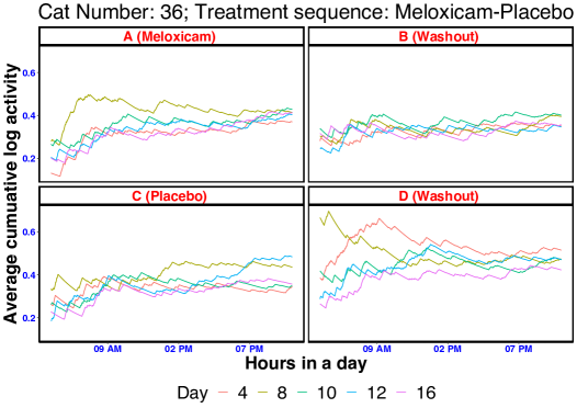
(a)

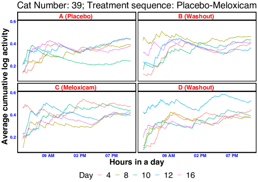
(b)

Figure 5: Cumulative average of the log activity profiles from $5$AM to $10$PM for two randomly selected cats (cat number $36$ and $39$) over the days $4,8,10,12$, and $16$ in all the four periods.

References

• Bussmann et al. (2001) Bussmann, J., Martens, W., Tulen, J., Schasfoort, F., Van Den Berg-Emons, H., and Stam, H. (2001). Measuring daily behavior using ambulatory accelerometry: the activity monitor. Behavior Research Methods, Instruments, & Computers 33, 349–356.
• Cochran et al. (1941) Cochran, W., Autrey, K., and Cannon, C. (1941). A double change-over design for dairy cattle feeding experiments. Journal of Dairy Science 24, 937–951.
• Crainiceanu and Ruppert (2004) Crainiceanu, C. M. and Ruppert, D. (2004). Likelihood ratio tests in linear mixed models with one variance component. Journal of the Royal Statistical Society: Series B 66, 165–185.
• Delaigle et al. (2016) Delaigle, A., Hall, P., and Zhou, W.-X. (2016). Nonparametric covariate-adjusted regression. The Annals of Statistics 44, 2190–2220.
• Di et al. (2009) Di, C.-Z., Crainiceanu, C. M., Caffo, B. S., and Punjabi, N. M. (2009). Multilevel functional principal component analysis. The Annals of Applied Statistics 3, 458.
• Freeman (1989) Freeman, P. (1989). The performance of the two-stage analysis of two-treatment, two-period crossover trials. Statistics in medicine 8, 1421–1432.
• Goldsmith et al. (2020) Goldsmith, J., Scheipl, F., Huang, L., Wrobel, J., Di, C., Gellar, J., Harezlak, J., McLean, M. W., Swihart, B., Xiao, L., Crainiceanu, C., and Reiss, P. T. (2020). refund: Regression with Functional Data. R package version 0.1-23.
• Goldsmith et al. (2015) Goldsmith, J., Zipunnikov, V., and Schrack, J. (2015). Generalized multilevel function-on-scalar regression and principal component analysis. Biometrics 71, 344–353.
• Gruen et al. (2015) Gruen, M. E., Griffith, E. H., Thomson, A. E., Simpson, W., and Lascelles, B. D. X. (2015). Criterion validation testing of clinical metrology instruments for measuring degenerative joint disease associated mobility impairment in cats. PLoS One 10, e0131839.
• Hills and Armitage (1979) Hills, M. and Armitage, P. (1979). The two-period cross-over clinical trial. British journal of clinical pharmacology 8, 7–20.
• Jones and Kenward (2014) Jones, B. and Kenward, M. G. (2014). Design and analysis of cross-over trials. Chapman and Hall/CRC.
• Koner et al. (2021) Koner, S., Park, S. Y., and Staicu, A.-M. (2021). Profit: Projection-based test in longitudinal functional data. arXiv preprint arXiv:2104.11355 .
• Mercer (1909) Mercer, J. (1909). Xvi. functions of positive and negative type, and their connection the theory of integral equations. Philosophical transactions of the royal society of London. Series A, containing papers of a mathematical or physical character 209, 415–446.
• Oh et al. (2019) Oh, S. et al. (2019). Significance tests for longitudinal functional data.
• Park and Staicu (2015) Park, S. Y. and Staicu, A.-M. (2015). Longitudinal functional data analysis. Stat 4, 212–226.
• Park et al. (2018) Park, S. Y., Staicu, A.-M., Xiao, L., and Crainiceanu, C. M. (2018). Simple fixed-effects inference for complex functional models. Biostatistics 19, 137–152.
• Pinheiro et al. (2021) Pinheiro, J., Bates, D., DebRoy, S., Sarkar, D., and R Core Team (2021). nlme: Linear and Nonlinear Mixed Effects Models. R package version 3.1-152.
• Ratkowsky et al. (1992) Ratkowsky, D., Alldredge, R., and Evans, M. A. (1992). Cross-over experiments: design, analysis and application, volume 135. CRC Press.
• Reider et al. (2020) Reider, L., Bai, J., Scharfstein, D. O., Zipunnikov, V., Investigators, M. O. S., et al. (2020). Methods for step count data: Determining “valid” days and quantifying fragmentation of walking bouts. Gait & Posture 81, 205–212.
• Ruppert et al. (2003) Ruppert, D., Wand, M. P., and Carroll, R. J. (2003). Semiparametric Regression. Cambridge university press.
• Scheffler et al. (2020) Scheffler, A., Telesca, D., Li, Q., Sugar, C. A., Distefano, C., Jeste, S., and Şentürk, D. (2020). Hybrid principal components analysis for region-referenced longitudinal functional eeg data. Biostatistics 21, 139–157.
• Senn (2002) Senn, S. (2002). Cross-over trials in clinical research, volume 5. John Wiley & Sons.
• Staicu et al. (2014) Staicu, A., Li, Y., Crainiceanu, C. M., and Ruppert, D. (2014). Likelihood ratio tests for dependent data with applications to longitudinal and functional data analysis. Scandinavian Journal of Statistics .
• Taylor and Karlin (2014) Taylor, H. M. and Karlin, S. (2014). An Introduction to Stochastic Modeling. Academic press.
• Wang and Chen (2012) Wang, Y. and Chen, H. (2012). On testing an unspecified function through a linear mixed effects model with multiple variance components. Biometrics 68, 1113–1125.
• Wood (2004) Wood, S. N. (2004). Stable and efficient multiple smoothing parameter estimation for generalized additive models. Journal of the American Statistical Association 99, 673–686.
• Xiao (2019) Xiao, L. (2019). Asymptotics of bivariate penalised splines. Journal of Nonparametric Statistics 31, 289–314.
• Xiao et al. (2020) Xiao, L. et al. (2020). Asymptotic properties of penalized splines for functional data. Bernoulli 26, 2847–2875.
• Xiao et al. (2015) Xiao, L., Huang, L., Schrack, J. A., Ferrucci, L., Zipunnikov, V., and Crainiceanu, C. M. (2015). Quantifying the lifetime circadian rhythm of physical activity: a covariate-dependent functional approach. Biostatistics 16, 352–367.
• Xiao et al. (2013) Xiao, L., Li, Y., and Ruppert, D. (2013). Fast bivariate p-splines: the sandwich smoother. Journal of the Royal Statistical Society: Series B pages 577–599.
• Zhang and Chen (2007) Zhang, J.-T. and Chen, J. (2007). Statistical inferences for functional data. The Annals of Statistics 35, 1052–1079.
• Zhang et al. (2016) Zhang, X., Wang, J.-L., et al. (2016). From sparse to dense functional data and beyond. The Annals of Statistics 44, 2281–2321.
• Zhang et al. (2019) Zhang, Y., Li, H., Keadle, S. K., Matthews, C. E., and Carroll, R. J. (2019). A review of statistical analyses on physical activity data collected from accelerometers. Statistics in biosciences 11, 465–476.
Supplementary Material for “PROLIFIC: Projection-based Test for Lack of Importance of Smooth Functional Effect in Crossover Design”