Molecular magnetism in the multi-configurational self-consistent field method

Abstract

We develop a structured theoretical framework used in our recent articles [Eur. Phys. J. B 92, 93 (2019) and Phys. Rev. B 101, 094427 (2020)] to characterize the unusual behavior of the magnetic spectrum, magnetization and magnetic susceptibility of the molecular magnet Ni₄Mo₁₂. The theoretical background is based on the molecular orbital theory in conjunction with the multi-configurational self-consistent field method and results in a post-Hartree-Fock scheme for constructing the corresponding energy spectrum. Furthermore, we construct a bilinear spin-like Hamiltonian involving discrete coupling parameters accounting for the relevant spectroscopic magnetic excitations, magnetization and magnetic susceptibility. The explicit expressions of the eigenenergies of the ensuing Hamiltonian are determined and the physical origin of broadening and splitting of experimentally observed peaks in the magnetic spectra is discussed. To demonstrate the efficiency of our method we compute the spectral properties of a spin-one magnetic dimer. The present approach may be applied to a variety of magnetic units based on transition metals and rare earth elements.

I Introduction

Since decades molecular magnets have secured their own place as prominent tools for gaining insights into the origin of magnetic exchange phenomena [1, 2, 3, 4, 5] and studying magneto-related effects [6, 7, 8, 9]. The magnetic properties of such small in size and isolated molecular units of matter are inevitably related to their size, symmetry, number and types of chemical bonds (for more details see [10, 11, 12, 13] and references therein). On the microscopic level, the low-spin and short-bridged magnetic compounds are ideal quantum systems for studying the origin of magneto-structural dependencies. Dimeric [14, 15, 16, 17] and trimeric [18, 19, 20] magnetic units are among the first and most widely explored sorts of spin clusters. In that regard, cooper based compounds have served as primordial tools in revealing the interdependence between exchange and structure parameters [21, 22, 23, 18, 24]. It is worth mentioning that, the relationship between bridging composition and magnetic exchange phenomena may be attributed to the study of different ligand bridged complexes with a variety of magnetic centers [25, 26, 27, 28, 29, 30]. Other prominent investigations related to the magneto-structural effects are complexes with Fe magnetic centers [31, 32, 33, 34, 35], Ni based compounds [36, 37, 38, 39, 40, 41] and Mn spin clusters [42, 43, 44, 45, 46, 47, 48].

For many isolated magnetic units that exhibit a mono or diatomic intermediate structure the ensuing exchange interactions may be approximately described by considering density functional theory, Hartree-Fock or non-sophisticated post-Hartree-Fock methods [49, 50, 51]. The electrons may be considered as localized. Thus the Goodenough-Kanamori-Anderson rules hold and the hopping and single-ion coulomb repulsion terms represent the leading electrons’ correlations. For such trivial bridging structure the analytical analysis allows the application of conventional microscopic spin models. Of particular interest are the Heisenberg and Hubbard models, since they possess just a few parameters to capture the main isotropic magnetic futures. On the other hand, any orbital contribution of the localized electrons into the exchange processes may require involving an anisotropic spin bilinear expression and/or including a single-ion anisotropy term accounting for the zero field splitting effect [1, 52].

In magnetic units with an intricate bridging structure [53, 54, 55] the mechanism of electrons’ exchange may involve a large number of intermediate atoms of different sorts. This imply that the correlations between electrons shared by individual metal centers contribute to the intrinsic magnetic features of these compounds. Thus, the constituent electrons are delocalized to a large extent occupying molecular orbitals. Depending on the spatial position of each metal center, the chemical composition of the bridges connecting two adjacent centers, the change in temperature and the action of external fields, the electrons’ distribution over the bridges may not be uniform. In other words, these compounds may allow multiple energetically favorable spin-orbital configurations giving rise to multiple independent magnetic excitations that are not related to local anisotropy effects nor to the existence of electronic bands. Studying the magnetic properties of these isolated molecular magnets requires the application of advanced methods, such as the multi-configurational self-consistent field. However, in contrast to single molecular magnets with trivial bridging structure and due to the lack of sufficient number of model parameters, the outcome of such advanced methods cannot be accounted for by conventional spin models. Neither the isotropic spin bilinear form nor higher-order spin interaction terms can account for all possible magnetic transitions and dependencies arising due to the delocalization of electrons. Moreover, neither the zero field splitting nor the exchange anisotropy terms are physically relevant to such process. Therefore, any attempt to gain insights into the existing exchange mechanisms by combining different conventional Hamiltonians will be inadequate.

The present paper develops a theoretical approach, used in our previous papers [56, 57, 58, 59], to determine the magnetic properties of isolated molecular magnets with non-trivial bridging structure. The named approach combines two widely used methods, namely the molecular orbital theory and the multi-configuration self-consistent field formalism resulting in a post-Hartree-Fock scheme for constructing the relevant energy spectrum. The main features of the ensuing energy sequence accounted for by constructing an effective spin-like microscopic model with a few adjustable running parameters. The named spin-like model was successfully applied to the identification of the magnetic spectra of the spin-half trimeric compounds family A₃Cu₃(PO₄)₄ A=(Ca, Sr, Pb) [57] and the spin-one tetrameric molecular magnet Ni₄Mo₁₂ [58]. A good agreement with inelastic neutron scattering experimental data was demonstrated. Furthermore, the ensuing model adequately reproduces the magnetization and low-field susceptibility measurements performed on the nickel tetramer Ni₄Mo₁₂ [59]. In contrast to conventional methods that require distinct spin Hamiltonians in order to explain the main features of each individual experiment, the constructed model includes a unique set of parameters for any experimental measurements.

The rest of the paper is organized as follows. In Sec. II we outline the basic principles of the molecular orbital theory and define the molecular orbitals to be further applied. In Sec. III we represent the mathematical formalism aiming to unveil the mechanisms of exchange and to quantify the magnetic properties in molecular magnets with non-trivial bridging structure. Thus, we introduce the total Hamiltonian and construct the variational functions. Moreover, we derive the corresponding effective matrices and compute the generalized energy spectrum. In Sec. IV we present the spin-like Hamiltonian accounting for the main features predicted by the applied variational method. Further, we discuss technical aspects of the relevant spin-like operators. A primer for the application of the proposed method and spin-like Hamiltonian is given in Sec. V. Section VI contains a summary of the introduced method and results.

II Molecular orbital theory

II.1 First principles

Nanomagnets possess unique properties with respect to their size and spatial symmetry and hence the corresponding chemical bonds length, angles and strength. These characteristics are a consequence of the overlap between pure or hybridized orbital states of the valence electrons interacting with each other and with the nuclei of the constituent atoms. The electrons distribute themselves in such a way to minimize the molecule’s total energy. Thus, the corresponding spatial distribution depends on the constituent electrons’ spin and therefore gives rise to a variety of magnetic effects.

There are two main theories describing chemical bonds in materials: the valence bond theory [60, 61, 62] and the molecular orbital theory [63, 64, 65, 66]. Both theories complement each other and successfully describe the quantum origin of chemical bonding. By analogy to the constructive and destructive interference when combining wave functions and with respect to the choice of internuclear axis the bonds are of two sorts: $\sigma$ and $\pi$ types. The strongest bonds are of $\sigma$ type and the associated electrons distributions are energetically more favorable.

The valence bond theory includes in the bonding processes only unpaired orbital electrons from the most outer shells and does not account for the contribution of the remaining paired valence electrons. Moreover, in explaining the chemical bonds, this theory regards the electrons as localized in between the constituent nuclei in pairs. Although, it is essential for the description of a multiple atomic molecule, it raises difficulties in explaining the behavior of paramagnetic molecules. Since magnetic exchange phenomena originate from the delocalization of electrons, such localized approach hinders the derivation of the full energy spectra of the exchange interactions. Thus, an alternative approach involving delocalized electrons may prove to be very useful. It lies on a basic principle of the molecular orbital theory, where the electrons are considered as spatially distributed over the entire molecule. Similar to the electron configurations in atoms, in molecular orbital theory electrons occupy molecular orbitals. Along these lines, the ligand field theory combines both the molecular orbital theory and the crystal field one to explain the electronic structure and spin state of coordination complexes [67] and to study the magnetic properties of larger magnetic clusters [30, 38, 19].

One way of constructing molecular orbitals is representing each one as a linear combination of atomic orbitals. Depending on the problem under consideration one may apply different approximations of atomic orbitals to minimize the energy, such as Hydrogen, Slater or Gaussian types [68, 50]. With respect to the type of bonds included in the construction of molecular orbitals, i.e. $\sigma$ and $\pi$ types, these are divided in three groups: bonding, antibonding and non-bonding. They are arranged in accordance to their energies. Lower in energy and hence most favorable are the bonding molecular orbitals, with energy less than that of the constituent atomic orbitals. Contrary, less energetically favorable are the antibonding molecular orbitals. Non-bonding orbitals have no contribution to the bond processes and have the same energy as the atomic orbitals they are constructed of. Moreover molecular orbitals are classified as core, active and virtual. Core orbitals are occupied by two electrons, also known as doubly or fully occupied by virtue of the Pauli exclusion principle. The second class, active molecular orbitals are those occupied by a single electron. They are also called half-filled. The virtual class represents the non-occupied molecular orbitals.

II.2 Molecular orbitals

In constructing the $i$-th electron molecular orbital state we assume that the corresponding atomic state taken with respect to the $\eta$-th constituent atom within the molecule is given by

$$\psi^{\eta}_{\mu_{i,\eta},m_{i}}(\mathbf{r}_{i})\equiv\psi^{\eta}_{\mu_{i,\eta}}(\mathbf{r}_{i})\lvert m_{i}\rangle,$$ (1)

where $\mu_{i,\eta}$ labels the shell and sub-shell that the $i$-th electron occupies on the $\eta$-th atom, $\mathbf{r}_{i}=(x_{i},y_{i},z_{i})$ and $m_{i}=\pm\tfrac{1}{2}$ are the $i$-th electron’s coordinates and spin-magnetic quantum number, respectively. For convenience the variational parameters in (1) are omitted. We would like to point out that in general the label $\mu_{i,\eta}$ may indicate either pure or hybridized atomic orbitals. For example, if the $i$-th electron occupies some of the three $2p$ orbitals in the $\eta$-th atom, then $\mu_{i,\eta}\in\{2p_{x},2p_{y},2p_{z}\}$ and the state in (1) will be rewritten as $\psi^{\eta}_{2p_{\alpha},m_{i}}(\mathbf{r}_{i})$, where $\alpha\in\mathbb{K}$. When the occupied orbital is a hybridization between $2s$ and $2p_{z}$ orbitals one has $\mu_{i,\eta}\in\{2sp^{\pm}_{z}\}$. Moreover, in the presence of an external magnetic field all orbitals are considered as gauge-invariant.

For all $\eta$ and $i$ the functions in (1) are orthogonal and normalized, i.e.,

$$\int\bar{\psi}^{\eta}_{\mu_{i,\eta},m_{i}}(\mathbf{r}_{i})\psi^{\eta}_{\mu^{\prime}_{i,\eta},m^{\prime}_{i}}(\mathbf{r}_{i})\mathrm{d}\mathbf{r}_{i}=\delta_{\mu_{i,\eta}\mu^{\prime}_{i,\eta}}\delta_{m_{i}m^{\prime}_{i}}.$$ (2)

Further, the overlap integral between any two arbitrary atomic states of the $i$-th electron residing on different atoms satisfies

$$0\leq\int\bar{\psi}^{\eta}_{\mu_{i,\eta},m_{i}}(\mathbf{r}_{i})\psi^{\eta^{\prime}}_{\mu^{\prime}_{i,\eta^{\prime}},m_{i}}(\mathbf{r}_{i})\mathrm{d}\mathbf{r}_{i}<1.$$ (3)

With respect to the state functions (1) and the Born–Oppenheimer approximation, we represent the $n$-th molecular orbital state of the $i$-th electron by

$$\phi_{n,m_{i}}(\mathbf{r}_{i})=\sum_{\eta}c^{\eta}_{n}\psi^{\eta}_{\mu_{i,\eta},m_{i}}(\mathbf{r}_{i}),$$ (4)

where the molecular orbital number $n$ is determined according to the symmetry of all atomic shells, sub-shells and the type of bonds, i.e. $\sigma$ and $\pi$ bonds. The coefficients $c^{\eta}_{n}$ are functions of the overlap integrals between the atomic orbitals, see (3). Employing the bra-ket notation in (1) the molecular orbital state representation (4) reads

$$\phi_{n,m_{i}}(\mathbf{r}_{i})\equiv\phi_{n}(\mathbf{r}_{i})\lvert m_{i}\rangle=\prod_{{\alpha\in\mathbb{K}}}\phi_{n}(\alpha_{i})\lvert m_{i}\rangle.$$ (5)

For all $i$ the molecular orbitals given in (4) are orthogonal,

$$\int\bar{\phi}_{n,m_{i}}(\mathbf{r}_{i})\phi_{n^{\prime},m^{\prime}_{i}}(\mathbf{r}_{i})\mathrm{d}\mathbf{r}_{i}=\delta_{nn^{\prime}}\delta_{m_{i}m^{\prime}_{i}}.$$ (6)

The arrangement of molecular orbitals in the energy diagram follows the value of $n$. According to the Aufbau principle their numeration is such that the lowest value of $n$ in (4) corresponds to the most energetically favorable molecular orbital. Thus, the first occupied molecular orbital should correspond the lowest level of the spectrum.

III Towards a post-Hartree-Fock method

Consider a molecular magnet composed of an arbitrary number of atoms. We have a multi particle non-relativistic system obeying the adiabatic approximation. Since the intrinsic electromagnetic field of the molecule, due to the presence of electrons and nuclei, includes static electric and magnetic components, henceforth we take into account only the dipole terms of the corresponding electron-electron and electron-nuclei interactions. We neglect the effect of all orbital-orbital, spin-spin and spin-orbital interactions between the electrons and atomic nuclei. The nuclei-nuclei potentials are also neglected, since for the considered system they do not contribute to the magnetic properties. Moreover the magnitude of the total magnetic vector potential is constant.

III.1 Electron’s generalized momentum

Let $\hat{\mathbf{p}}_{i}=(p^{\alpha}_{i})_{\alpha\in\mathbb{K}}$ be the $i$-th electron’s momentum operator with coordinates $\mathbf{r}_{i}=(\alpha_{i})_{\alpha\in\mathbb{K}}$, $\hat{\boldsymbol{s}}_{i}=(\hat{s}^{\alpha}_{i})_{\alpha\in\mathbb{K}}$ and $\hat{\boldsymbol{l}}_{i}=(\hat{l}^{\alpha}_{i})_{\alpha\in\mathbb{K}}$ are, respectively, the corresponding spin and angular momentum operators, where $\mathbb{K}=\{x,y,z\}$ and $i=1,\ldots,N$. Furthermore, let $\hat{\boldsymbol{\mu}}_{l_{i}}=-\mu_{\mathrm{B}}\hat{\boldsymbol{l}}_{i}$ and $\hat{\boldsymbol{\mu}}_{s_{i}}=-g_{s}\mu_{\mathrm{B}}\hat{\boldsymbol{s}}_{i}$ be the orbital and spin magnetic moments of the $i$-th electron, where $\mu_{\mathrm{B}}=e\hbar/2m_{e}$ is the Bohr magneton with $m_{e}$ denoting electron’s rest mass. The action of an external magnetic and the cluster’s intrinsic magnetic fields into the $i$-th electron momentum is accounted for by means of the generalized momentum operator $\hat{\mathbf{P}}_{i}=\hat{\mathbf{p}}_{i}-e\hat{\mathbf{A}}(\mathbf{r}_{i})$, where $\hat{\mathbf{A}}(\mathbf{r}_{i})=(\hat{A}_{\alpha}(\mathbf{r}_{i}))_{\alpha\in\mathbb{K}}$ is the operator related to the total magnetic vector potential at a point with coordinates $\mathbf{r}_{i}$. We have

$$\hat{\mathbf{A}}(\mathbf{r}_{i})=\hat{\mathbf{A}}_{ext}(\mathbf{r}_{i})+\sum_{j|_{j\neq i}}\hat{\mathbf{A}}(\mathbf{r}_{ij}),$$ (7)

where $\mathbf{r}_{ij}$ is the vector of the distance between $i$-th and $j$-th electrons. In equation (7), $\hat{\mathbf{A}}_{ext}=\big{(}\hat{A}^{\alpha}_{ext}(\mathbf{r}_{i})\big{)}_{\alpha\in\mathbb{K}}$, for $\hat{\mathbf{A}}_{ext}\equiv\mathbf{A}_{ext}$, represents the magnetic vector potential associated to the externally applied magnetic field $\mathbf{B}=(B_{\alpha})_{\alpha\in\mathbb{K}}$ and $\hat{\mathbf{A}}(\mathbf{r}_{ij})=\big{(}\hat{A}_{\alpha}(\mathbf{r}_{ij})\big{)}_{\alpha\in\mathbb{K}}$ the magnetic vector potential related to the orbital angular momentum operator of the $j$-th electron. In other words, under the considered approximations, we have

$$\mathbf{A}_{ext}(\mathbf{r})=\frac{1}{2}\mathbf{B}\times\mathbf{r}$$ (8a)

and

$$\hat{\mathbf{A}}(\mathbf{r}_{ij})=\frac{\mu_{0}\mu_{\mathrm{B}}}{4\pi^{2}\langle r_{ij}\rangle^{3}}\mathbf{r}_{ij}\times(\hat{\boldsymbol{l}}_{j}+g_{s}\hat{\boldsymbol{s}}_{j}),$$ (8b)

where $\mu_{0}$ is the magnetic permeability in vacuum, $r_{ij}=|\mathbf{r}_{i}-\mathbf{r}_{j}|$ is the distance between $i$-th and $j$-th electrons and $\mathbf{r}\in\{\mathbf{r}_{1},\ldots,\mathbf{r}_{N}\}$. The average $\langle r_{ij}\rangle$ is taken with respect to the molecular orbitals $i$-th and $j$-th electrons occupy.

Therefore, since for all $\alpha$ and $i$ the operators $\hat{A}_{\alpha}(\mathbf{r}_{i})$ and $\hat{p}^{\alpha}_{i}$ commute, with respect to equations (7) and (8) the generalized momentum operator reads

$$\hat{\mathbf{P}}^{2}_{i}= \ \hat{\mathbf{p}}^{2}_{i}+2m_{e}\!\!\sum_{j|_{j\neq i}}\hat{K}^{l}_{ij}+2m_{e}\!\!\sum_{j|_{j\neq i}}\hat{K}^{s}_{ij}$$

$$-2m_{e}\mu_{\mathrm{B}}\mathbf{B}\cdot\hat{\boldsymbol{l}}_{i}+\frac{e^{2}}{4}\mathbf{B}^{2}\mathbf{r}^{2}_{i},$$ (9a)

where

$$\hat{K}^{l}_{ij}= -\frac{\mu_{0}\mu^{2}_{\mathrm{B}}}{2\pi^{2}\langle r_{ij}\rangle^{3}}\hat{\boldsymbol{l}}_{i}\cdot\hat{\boldsymbol{l}}_{j}$$

$$+\frac{e^{2}\mu_{0}\mu_{\mathrm{B}}}{8m_{e}\pi^{2}\langle r_{ij}\rangle^{3}}\bigg{[}\left(\mathbf{r}_{ij}\cdot\mathbf{B}\right)\left(\mathbf{r}_{i}\cdot\hat{\boldsymbol{l}}_{j}\right)-\left(\mathbf{r}_{i}\cdot\mathbf{r}_{ij}\right)\left(\mathbf{B}\cdot\hat{\boldsymbol{l}}_{j}\right)\bigg{]},$$ (9b)

$$\hat{K}^{s}_{ij}= -\frac{\mu_{0}\mu^{2}_{\mathrm{B}}g_{s}}{2\pi^{2}\langle r_{ij}\rangle^{3}}\hat{\boldsymbol{l}}_{i}\cdot\hat{\boldsymbol{s}}_{j}$$

$$+\frac{e^{2}\mu_{0}\mu_{\mathrm{B}}g_{s}}{8m_{e}\pi^{2}\langle r_{ij}\rangle^{3}}\bigg{[}\left(\mathbf{r}_{ij}\cdot\mathbf{B}\right)\left(\mathbf{r}_{i}\cdot\hat{\boldsymbol{s}}_{j}\right)-\left(\mathbf{r}_{i}\cdot\mathbf{r}_{ij}\right)\left(\mathbf{B}\cdot\hat{\boldsymbol{s}}_{j}\right)\bigg{]}.$$ (9c)

For further details on the representation of the $i$-th electron’s general momentum operator in (9), the interested reader may consult Appendix A.1 and Refs. [69, 70].

III.2 The canonical Hamiltonian

According to all assumptions and definitions in Sec. III.1, the Hamiltonian accounting for all interactions in the considered system reads

$$\hat{H}=\sum_{i}\frac{{\hat{\mathbf{P}}^{2}_{i}}}{2m_{e}}+\sum_{\eta,i}\hat{U}_{\eta i}+\frac{1}{2}\sum_{i\neq j}\hat{R}_{ij}-g_{s}\mu_{\mathrm{B}}\sum_{i}\mathbf{B}\cdot\hat{\boldsymbol{s}}_{i},$$ (10)

where the potential energy operator $\hat{U}_{\eta i}\equiv U(r_{\eta i})$ accounts for the interaction of the $i$-th electron with the $\eta$-th nucleus, separated by the distance $r_{\eta i}=|\mathbf{r}_{i}-\mathbf{R}_{\eta}|$, with $\mathbf{R}_{\eta}$ representing the coordinates of the $\eta$-th nucleus. The operator $\hat{R}_{ij}\equiv R(r_{ij})$ is related to the repulsion potential between $i$-th and $j$-th electrons over the distance $r_{ij}=|\mathbf{r}_{i}-\mathbf{r}_{j}|$.

Taking into account equations (9), Hamiltonian (10) can be represented as the sum of three terms, i.e.

$$\hat{H}=\hat{H}_{r}+\hat{H}_{l}+\hat{H}_{s},$$ (11)

where the spin-independent part of the total Hamiltonian is given by

$$\hat{H}_{r}= \sum_{i}\frac{{\hat{\mathbf{p}}^{2}_{i}}}{2m_{e}}+\sum_{\eta,i}\hat{U}_{\eta i}+\sum_{i\neq j}\frac{1}{2}\hat{R}_{ij}-\sum_{i}\frac{e^{2}}{8m_{e}}\mathbf{B}^{2}\mathbf{r}^{2}_{i},$$ (12a)

the orbital term reads

$$\hat{H}_{l}=\sum_{i\neq j}\hat{K}^{l}_{ij}-\mu_{\mathrm{B}}\sum_{i}\mathbf{B}\cdot\hat{\boldsymbol{l}}_{i}$$ (12b)

and the spin one is

$$\hat{H}_{s}=\sum_{i\neq j}\hat{K}^{s}_{ij}-g_{s}\mu_{\mathrm{B}}\sum_{i}\mathbf{B}\cdot\hat{\boldsymbol{s}}_{i}.$$ (12c)

For $|\mathbf{B}|>0$, the orbital bilinear form in (9) and the spin-orbit form in (9) are negligibly small compared to the other terms. As a result, the expressions of the respective Hamiltonians given in (12b) and (12c) simplify. Thus, We have

$$\hat{H}_{l}=-\mu_{\mathrm{B}}B\sum^{N}_{i=1}\boldsymbol{g}_{i}\cdot\hat{\boldsymbol{l}}_{i}$$ (13)

and

$$\hat{H}_{s}=-g_{s}\mu_{\mathrm{B}}B\sum^{N}_{i=1}\boldsymbol{g}_{i}\cdot\hat{\boldsymbol{s}}_{i},$$ (14)

where $\mathbf{B}=\mathbf{n}B$, $\mathbf{n}=(n_{\alpha})_{{\alpha\in\mathbb{K}}}$ is a unit vector and the $\boldsymbol{g}$ factor reads

$$\boldsymbol{g}_{i}=\left(\mathbf{n}-\sum_{j|_{j\neq i}}\frac{e^{2}\mu_{0}}{8m_{e}\pi^{2}\langle r_{ij}\rangle^{3}}\bigg{[}\mathbf{r}_{j}\left(\mathbf{r}_{ij}\cdot\mathbf{n}\right)-\mathbf{n}\left(\mathbf{r}_{j}\cdot\mathbf{r}_{ij}\right)\bigg{]}\right),$$ (15)

with $\boldsymbol{g}_{i}=(g^{\alpha}_{i})_{\alpha\in\mathbb{K}}$.

III.3 State functions

Studying the magnetic behavior of a molecule with complex bridging structures we apply the molecular orbital theory and construct the variational state function within the multi-configurational self-consistent field method. Thus, selecting $\alpha\in\mathbb{K}$ axis as a quantization axis, we describe an arbitrary spin configuration of $N$ number of electrons, occupying $n$ molecular orbitals given in (4), by

$$\Psi^{1,\ldots,n-1,n}_{m_{1},\ldots,m_{N}}(\mathbf{r}_{1},\ldots,\mathbf{r}_{N})= \sum_{P_{\mathbf{r}_{1},\ldots,\mathbf{r}_{N}}}c_{\mathbf{r}_{1},\ldots,\mathbf{r}_{N}}\phi_{1,m_{1}}(\mathbf{r}_{1})\phi_{1,m_{2}}(\mathbf{r}_{2})$$

$$\cdots\phi_{{n-1},m_{N-1}}(\mathbf{r}_{N-1})\phi_{n,m_{N}}(\mathbf{r}_{N}),$$ (16)

where $n-1$ and $n$ are the highest in energy active molecular orbitals, the sum runs over all permutations on the set of coordinates $\mathbf{r}_{1},\ldots,\mathbf{r}_{N}$, the coefficients $c_{\mathbf{r}_{1},\ldots,\mathbf{r}_{N}}$ account for the orthonormalization and antisymmetry of the state function and the set $\{m_{1},\ldots,m_{N}\}$ identifies the spin configuration according to the selected quantization axis. Each function in (III.3) corresponds to a single Slater determinant.

In general, all $N$ electrons are involved in the exchange process. However, as the core molecular orbitals are permanently occupied by two electrons the total spin multiplet scheme of the system is generated with respect to the number of all active and post-active orbitals. Furthermore, since a triplet-singlet transition of an electron spin pair requires two active orbitals each individual spin multiplet relates to certain pairs of such orbitals. Therefore, let $\tau\in\{(n-i,n-j),\ldots,(n-1,n)\}$ indicate all pairs or a tuple of pairs of active orbitals, with $i\neq j=2,3\ldots,n-(\bar{n}+1)$, where $\bar{n}$ is the number of the highest in energy core molecular orbital. Then, the generalized state function representing a spin multiplet related to the pair of active orbitals $\tau=(n-1,n)$ is given by the following superposition of the basis states in (III.3)

$$\Psi^{\tau,v_{\tau,s_{\tau},s}}_{s_{\tau},s,m}(\mathbf{r}_{1},\ldots,\mathbf{r}_{N})= \sum_{m_{1}=-s_{1}}^{s_{1}}\!\ldots\!\sum_{m_{N}=-s_{N}}^{s_{N}}c^{s_{\tau},s,m}_{m_{1},\ldots,m_{N}}$$

$$\times\!\!\!\sum_{n-1,n}{c^{v_{\tau,s_{\tau},s}}_{n-1,n}}\Psi^{1,\ldots,n-1,n}_{m_{1},\ldots,m_{N}}(\mathbf{r}_{1},\ldots,\mathbf{r}_{N}),$$ (17)

where $c^{s_{\tau},s,m}_{m_{1},\ldots,m_{N}}$ are the Clebsch-Gordan coefficients, the scalars $c^{v_{\tau,s_{\tau},s}}_{n-i,n}$ symmetrize the state function with respect to all energetically equivalent orbitals within the considered pair or a tuple of pairs, with $v_{\tau,s_{\tau},s}\in\mathbb{N}$ indicating all linearly independent combinations, $s$ and $m$ denote the system’s total spin quantum numbers and $s_{\tau}\equiv s_{n-1,n}$ the local spin quantum number related to both active orbitals. We would like to point out that in both (III.3) and (III.3) there is a sum running over the permutation of all electrons. As a result, the quantum number $s_{n-1,n}$ will represent the spin quantum number of each electron pair occupying the orbitals $n-1$ and $n$. Furthermore, the array of subscripts $s_{\tau},s,m$ is a shorthand notation of the resulting spin multiplet represented by all good spin quantum numbers $\{s_{n-i,n-j},\ldots,s_{n-1,n},s,m\}$. For the sake of clarity we use only spin quantum number relevant to all active orbitals. For example, if the configuration includes four active orbitals, with $\tau=\{(n-3,n-2),(n-1,n)\}$, then the set $s_{\tau},s,m$ should be rewritten as $s_{n-3,n-2},s_{n-1,n},s,m$, see also Appendix A.2.

The number of all sets of molecular orbitals involved in the exchange processes $\tau$ increases with the number of all intermediate bridges. Respectively, the number of all state functions in (III.3) will depend on all distinct electrons’ distributions and hence spin-orbital configurations indicated by the index $\tau$. The electrons’ correlations for any such distribution are taken into account with respect to the effective Hamiltonian $\hat{H}_{\mathrm{eff}}=\hat{H}^{r}_{\mathrm{eff}}+\hat{H}^{l}_{\mathrm{eff}}+\hat{H}^{s}_{\mathrm{eff}}$ to the initial Hamiltonian given in (11), that accounts for the energy levels degeneracy with regard to the spatial and spin components of the considered state functions. The effective semi-spin states, corresponding to these given in (III.3), read $\lvert\Psi^{\tau,v_{\tau,s_{\tau},s}}_{s_{\tau},s,m}\rangle$. Hence, constructing the total effective matrix, we have

$$\Big{\langle}\Psi^{\tau,v_{\tau,s_{\tau},s}}_{s_{\tau},s,m}\Big{\rvert}\hat{H}_{\mathrm{eff}}\Big{\lvert}\Psi^{\tau,v_{\tau,s_{\tau},s}}_{s_{\tau},s,m}\Big{\rangle}\equiv \int\!\cdots\!\int\bar{\Psi}^{\tau,v_{\tau,s_{\tau},s}}_{s_{\tau},s,m}(\mathbf{r}_{1},\ldots,\mathbf{r}_{N})\hat{H}$$

$$\times\Psi^{\tau,v_{\tau,s_{\tau},s}}_{s_{\tau},s,m}(\mathbf{r}_{1},\ldots,\mathbf{r}_{N})\mathrm{d}\mathbf{r}_{1}\cdots\mathrm{d}\mathbf{r}_{N}.$$ (18)

Since Hamiltonian (10) accounts for only pair interactions and the terms $\hat{H}_{r}$ and $\hat{H}_{l}$ act only on the spatial component of (III.3), the effective matrices associated to $\hat{H}^{r}_{\mathrm{eff}}$ and $\hat{H}^{l}_{\mathrm{eff}}$ will have off-diagonal terms only with respect to $v_{\tau,s_{\tau},s}$. Accordingly, the diagonalization of the total matrix related to $\hat{H}_{\mathrm{eff}}$ will mix the elements of both matrices associated to $\hat{H}^{r}_{\mathrm{eff}}$ and $\hat{H}^{l}_{\mathrm{eff}}$. As a result, in diagonal form we have $\hat{H}_{\mathrm{eff}}\to\hat{\mathrm{H}}^{r,l}_{\mathrm{eff}}+\hat{\mathrm{H}}^{s}_{\mathrm{eff}}$, such that

$$\hat{\mathrm{H}}^{r,l}_{\mathrm{eff}}\big{\lvert}\Omega^{\tau,n_{\tau,s_{\tau},s}}_{s_{\tau},s,m}\big{\rangle}=E^{\mathrm{f},(n_{\tau,s_{\tau},s})}_{\tau,s_{\tau},s,m}\big{\lvert}\Omega^{\tau,n_{\tau,s_{\tau},s}}_{s_{\tau},s,m}\big{\rangle},$$ (19a)

$$\hat{\mathrm{H}}^{s}_{\mathrm{eff}}\big{\lvert}\Omega^{\tau,n_{\tau,s_{\tau},s}}_{s_{\tau},s,m}\big{\rangle}=\mathcal{E}^{(n_{\tau,s_{\tau},s})}_{\tau,s_{\tau},s,m}\big{\lvert}\Omega^{\tau,n_{\tau,s_{\tau},s}}_{s_{\tau},s,m}\big{\rangle},$$ (19b)

where the index $n_{\tau,s_{\tau},s}\in\mathbb{N}$ runs over the corresponding subset of all eigenstates given by

$$\big{\lvert}\Omega^{\tau,n_{\tau,s_{\tau},s}}_{s_{\tau},s,m}\big{\rangle}={\sum_{v_{\tau,s_{\tau},s}}c^{v_{\tau,s_{\tau},s}}_{n_{\tau,s_{\tau},s}}\big{\lvert}\Psi^{\tau,v_{\tau,s_{\tau},s}}_{s_{\tau},s,m}\big{\rangle}}.$$ (20)

and the superscript “f” indicates that in the case $B\neq 0$ the eigenvalues (19a) are functions of the externally applied magnetic field. Notice that after diagonalization the initial Hilbert space relevant to (III.3) is reduced and the eigenstates (19) take into account only the spins related to the active molecular orbitals.

Due to the existence of different spin-orbital configurations indicated by the indexes $\tau$ and $n_{\tau,s_{\tau},s}$, for a given total spin $s$ the basis set of all functions in (20) includes an array of spin multiplets each distinguished by the quantum numbers $s_{\tau}$. Therefore, in constructing the final effective spin space we incorporate the contributions of all individual spin multiplets, $(\ldots,s_{\tau},s,m),(\ldots,s^{\prime}_{\tau},s,m)\ldots,(\ldots,s^{\prime}_{\tau^{\prime}},s,m)$, by introducing the following superposition

$$\lvert s,m\rangle=\sum_{[\ldots,s_{\tau}]}\sum_{\tau,n_{\tau,s_{\tau},s}}c^{(n_{\tau,s_{\tau},s})}_{\tau,s_{\tau},s,m}\big{\lvert}\Omega^{\tau,n_{\tau,s_{\tau},s}}_{s_{\tau},s,m}\big{\rangle},$$ (21)

where the coefficients $c^{(n_{\tau,s_{\tau},s})}_{\tau,s_{\tau},s,m}$ are associated to the probability weights accounting for the contribution of each energetically distinct spin-orbital configuration labeled by $\tau$ and $n_{\tau,s_{\tau},s}$ for observing the system in a spin state characterized by the total quantum numbers $s$ and $m$. At each total spin level, the first sum, with $[\ldots,s_{\tau}]$ in (21), runs only over the local spin quantum numbers related to the selected active molecular orbitals. For example, if we consider four active orbitals with $\tau=\{(n-3,n-2),(n-1,n)\}$, then the sum will run over all values of $s_{n-3,n-2}$ and $s_{n-1,n}$, where $|s_{n-3,n-2}+s_{n-1,n}|\geq s\geq|s_{n-3,n-2}-s_{n-1,n}|$. Therefore, in contrast to (20) the Hilbert space dimension associated to (21) is reduced to a large extent rendering the analytical computation with an appropriately parametrized spin model more tractable.

III.4 Key integrals

In the presence of an external magnetic field the energy of each molecular orbital shifts and hence the values of all exchange integrals alter. Moreover, the indirect action of $\mathbf{B}$ on the electrons’ correlations is taken into account by the field-dependent eigenvalues (19a), where the diamagnetic terms (12a) and the paramagnetic ones (12b) contribute with different weights to these effective matrix’s diagonal elements.

Within th convention, the post-coulomb integral referring to the $(N-1)$-th and $N$-th electrons occupying the $n$-th molecular orbital, with $n=N/2$, reads

$$U_{n}=\iint\bar{\phi}_{n}(\mathbf{r}_{N-1})\bar{\phi}_{n}(\mathbf{r}_{N})\hat{H}^{\prime}_{r,l}\phi_{n}(\mathbf{r}_{N-1})\phi_{n}(\mathbf{r}_{N})\mathrm{d}\mathbf{r}_{N-1}\mathrm{d}\mathbf{r}_{N},$$ (22a)

where

$$\hat{H}^{\prime}_{r,l}= \prod_{i,j}^{\tfrac{N}{2}-1}\int\!\!\cdots\!\!\int\bar{\phi}_{j}(\mathbf{r}_{2j-1})\bar{\phi}_{j}(\mathbf{r}_{2j})(\hat{H}_{r}+\hat{H}_{l})$$

$$\times\phi_{i}(\mathbf{r}_{2i-1})\phi_{i}(\mathbf{r}_{2i})\mathrm{d}\mathbf{r}_{1}\cdots\mathrm{d}\mathbf{r}_{N-2},$$ (22b)

is the Hamiltonian associated to the energy of $$(N-1) N \hat{H}^{\prime}_{r,l}$$-th and -th electrons interacting with the averaged field of all remaining electrons. Hamiltonian incorporates all correlations related to the lowest in energy core molecular orbitals.

The post-hopping integral corresponding to the same electrons, with $N$-th one hopping between $n$-th and $n^{\prime}$-th molecular orbitals, is given by

$$t_{nn^{\prime}}=\iint\bar{\phi}_{n}(\mathbf{r}_{N-1})\bar{\phi}_{n}(\mathbf{r}_{N})\hat{H}^{\prime}_{r,l}\phi_{n}(\mathbf{r}_{N-1})\phi_{n^{\prime}}(\mathbf{r}_{N})\mathrm{d}\mathbf{r}_{N-1}\mathrm{d}\mathbf{r}_{N},$$ (22c)

where $n^{\prime}=N/2-k$, for $k\in\mathbb{N}$. In particular, according to the Hund’s rule, $k=1$. When both electrons occupy different orbitals, we have the second coulomb integral

$$V_{nn^{\prime}}=\iint\bar{\phi}_{n}(\mathbf{r}_{N-1})\bar{\phi}_{n^{\prime}}(\mathbf{r}_{N})\hat{H}^{\prime}_{r,l}\phi_{n}(\mathbf{r}_{N-1})\phi_{n^{\prime}}(\mathbf{r}_{N})\mathrm{d}\mathbf{r}_{N-1}\mathrm{d}\mathbf{r}_{N}.$$ (22d)

The direct exchange integral associated to the direct exchange of $(N-1)$-th and $N$-th electrons between orbitals $n$ and $n^{\prime}$ is

$$D_{nn^{\prime}}=\iint\bar{\phi}_{n}(\mathbf{r}_{N-1})\bar{\phi}_{n^{\prime}}(\mathbf{r}_{N})\hat{H}^{\prime}_{r,l}\phi_{n^{\prime}}(\mathbf{r}_{N-1})\phi_{n}(\mathbf{r}_{N})\mathrm{d}\mathbf{r}_{N-1}\mathrm{d}\mathbf{r}_{N}.$$ (22e)

After implicit summation over all electrons and probability coefficients in (III.3), integrals (22) determine the eigenvalues (19a) accordingly.

All eigenvalues in (19b) account for the direct action of the externally applied magnetic field, such that from (14) we have

$$\mathcal{E}^{(n_{\tau,s_{\tau},s})}_{\tau,s_{\tau},s,m}=-\mu_{\mathrm{B}}B\sum^{N}_{i=1}\langle g^{\alpha}_{i}\rangle^{(n_{\tau,s_{\tau},s})}_{\tau,s_{\tau},s}\langle\hat{s}^{\alpha}_{i}\rangle_{s_{\tau},s,m},$$ (23)

where the electron’s $g_{s}$-factor is implicitly included in the corresponding average and with respect to the preselected quantization axis $\alpha$, $\langle\hat{\boldsymbol{s}}_{i}\rangle_{s_{\tau},s,m}\to\langle\hat{s}^{\alpha}_{i}\rangle_{s_{\tau},s,m}$. Notice that depending on the existing spin-orbital configurations, after diagonalization, for all $\alpha$ the average value of the $g$-factor in (23) may be a function of multiple average values $\langle g^{\alpha}_{i}\rangle^{(v_{\tau,s_{\tau},s})}_{\tau,s_{\tau},s}$ entering in (III.3), with $v_{\tau,s_{\tau},s}\in\mathbb{N}$.

III.5 Energy spectrum

In obtaining the energy sequence corresponding to the total effective spin space (21) we take into account the temperature at which measurements take place and imply the relation

$$E^{\mathrm{f}}_{s,m}=\langle s,m\rvert\hat{\rho}_{s,m}\left(\hat{\mathrm{H}}^{r,l}_{\mathrm{eff}}+\hat{\mathrm{H}}^{s}_{\mathrm{eff}}\right)\lvert s,m\rangle,$$ (24)

where the operator

$$\hat{\rho}_{s,m}=\sum_{[\ldots,s_{\tau}]}\sum_{\tau,n_{\tau,s_{\tau},s}}\rho^{(n_{\tau,s_{\tau},s})}_{\tau,s_{\tau},s,m}\delta_{\tau\tau^{\prime}}\delta_{s_{\tau}s^{\prime}_{\tau}}\delta_{n_{\tau,s_{\tau},s}n^{\prime}_{\tau,s_{\tau},s}}$$ (25)

accounts for the probability distribution for observing the system in a state with given energy at given temperature. In terms of the Boltzmann distribution, we have

$$\rho^{(n_{\tau,s_{\tau},s})}_{\tau,s_{\tau},s,m}=Z^{-1}e^{-\beta\varSigma^{\mathrm{f},(n_{\tau,s_{\tau},s})}_{\tau,s_{\tau},s,m}},$$ (26)

where $\beta=1/\kappa_{B}T$ (with $\kappa_{B}$ the Boltzmann constant), the partition function

$$Z=\sum_{\tau,n_{\tau,s_{\tau},s}}\ \sum_{s_{\tau},s,m}e^{-\beta\varSigma^{\mathrm{f},(n_{\tau,s_{\tau},s})}_{\tau,s_{\tau},s,m}}$$

and

$$\varSigma^{\mathrm{f},(n_{\tau,s_{\tau},s})}_{\tau,s_{\tau},s,m}=E^{\mathrm{f},(n_{\tau,s_{\tau},s})}_{\tau,s_{\tau},s,m}+\mathcal{E}^{(n_{\tau,s_{\tau},s})}_{\tau,s_{\tau},s,m}.$$ (27)

Now, accounting for (24), (25) and (27), for the effective energy spectrum we get

$$E^{\mathrm{f}}_{s,m}=\sum_{[\ldots,s_{\tau}]}\sum_{\tau,n_{\tau,s_{\tau},s}}\left|c^{(n_{\tau,s_{\tau},s})}_{\tau,s_{\tau},s,m}\right|^{2}\rho^{(n_{\tau,s_{\tau},s})}_{\tau,s_{\tau},s,m}\varSigma^{\mathrm{f},(n_{\tau,s_{\tau},s})}_{\tau,s_{\tau},s,m}.$$ (28)

Hence, an arbitrary energy gap in the obtained spectrum is given by

$$\left|E^{\mathrm{f}}_{\Delta s,\Delta m}\right|= \left|\sum_{\tau}\left(\sum_{[\ldots,s_{\tau}]}\sum_{n_{\tau,s_{\tau},s}}\left|c^{(n_{\tau,s_{\tau},s})}_{\tau,s_{\tau},s,m}\right|^{2}\rho^{(n_{\tau,s_{\tau},s})}_{\tau,s_{\tau},s,m}\varSigma^{\mathrm{f},(n_{\tau,s_{\tau},s})}_{\tau,s_{\tau},s,m}\right.\right.$$

$$\left.\left.-\sum_{[\ldots,s^{\prime}_{\tau}]}\sum_{n_{\tau,s^{\prime}_{\tau},s^{\prime}}}\left|c^{(n_{\tau,s^{\prime}_{\tau},s^{\prime}})}_{\tau,s^{\prime}_{\tau},s^{\prime},m^{\prime}}\right|^{2}\rho^{(n_{\tau,s^{\prime}_{\tau},s^{\prime}})}_{\tau,s^{\prime}_{\tau},s^{\prime},m^{\prime}}\varSigma^{\mathrm{f},(n_{\tau,s^{\prime}_{\tau},s^{\prime}})}_{\tau,s^{\prime}_{\tau},s^{\prime},m^{\prime}}\right)\right|,$$ (29)

where $\Delta s=s-s^{\prime}$ and $\Delta m=m-m^{\prime}$. Within the last relation one has to bear in mind that the transitions between states characterized by a same local spin quantum number $s_{\tau}$ are forbidden. Consequently, the energy of a magnetic transition associated to $\Delta s$ and $\Delta m$ will vary in accordance to each spin-orbital configuration indicated by $\tau$ and $n_{\tau,s_{\tau},s}$.

IV The spin-sigma Hamiltonian

A magnetic molecule with a particular size, symmetry and complexity of the intermediate bridging structure among the magnetic centers may exhibits a unique set of energetically favorable electrons’ distributions. Accordingly, being exposed to an external action it may respond uniquely in revealing its magnetic properties. On the theoretical side, the relevant magnetic features could be studied with the aid of the post-Hartree-Fock method discussed in Section III and a spin Hamiltonian adequate to the computation of the energy spectrum (28). Since the spectrum in (28) consists of two independent components, we have to rely on two different spin terms. One Hamiltonian addressing the exchange interactions relevant to the eigenvalues (19a) and a Zeeman term incorporating the direct action of the external magnetic field according to energy eigenvalues in (19b).

Within the considered method, due to the small number of effective parameters, spin bilinear Hamiltonians, such as the Heisenberg model, may not account for all probable transitions in (III.5) at zero magnetic field, $|\mathbf{B}|=0$. Respectively, the effective energy spectrum obtained with any such Hamiltonian will represent only a small fragment of the full energy sequence relevant to the possible exchange processes. Further, for $|\mathbf{B}|\neq 0$ the conventional spin Zeeman term cannot be used within the present method, since the spectroscopic $g$-tensor is derived based on different physical reasoning. Under this circumstances, some splittings and broadening of the non-magnetic peaks in the corresponding magnetic spectrum may remain unexplained or erroneously attributed to the magnetic anisotropy. Therefore, as it was argued in Sec. I any attempt to describe such effects by adding different magneto-anisotropic terms or higher-order spin interaction terms to the Heisenberg model will not be physically adequate.

To identify all possible transitions described by (III.5), we need at hand an appropriate bilinear spin interaction form and a field term with eigenstates relevant to (21). To this end, we propose the following Hamiltonians

$$\hat{\mathcal{H}}_{\sigma}=\sum\limits_{i\neq j}J_{ij}\hat{\boldsymbol{\sigma}}_{i}\cdot\hat{\mathbf{s}}_{j}$$ (30a)

and

$$\hat{\mathcal{H}}_{Z}=-\mu_{\mathrm{B}}B\sum_{i}\hat{S}^{\alpha}_{i}$$ (30b)

where the couplings $J_{ij}=J_{ji}$ are effective exchange constants, $\hat{\mathbf{s}}_{i}=(\hat{\mathrm{s}}^{\alpha}_{i})_{\alpha\in\mathbb{K}}$, is the spin operator of the $i$-th effective magnetic center, for all $\alpha$ the sigma operator $\hat{\boldsymbol{\sigma}}_{i}=(\hat{\sigma}^{\alpha}_{i})_{\alpha\in\mathbb{K}}$ and $\hat{S}^{\alpha}_{i}$ are functions of the $i$-th effective spin discussed hereafter.

In particular, Hamiltonian (30a) maps the energy gaps given in (III.5) only with respect to the terms $E^{\mathrm{f},(n_{\tau,s_{\tau},s})}_{\tau,s_{\tau},s,m}$. The explicit representation and hence the physical meaning of all $J$-couplings differ from those entering the Heisenberg Hamiltonian. Moreover, as the energy terms $E^{\mathrm{f},(n_{\tau,s_{\tau},s})}_{\tau,s_{\tau},s,m}$ are field dependent the sigma operator aim to generate two sets of parameters. The first one accounts for all transitions related to the probability amplitudes and distribution probabilities (III.5) for $|\mathbf{B}|=0$. The second set indicates the changes in all electrons’ correlations due to the contribution of external magnetic field.

Hamiltonian (30b) represents the Zeeman term and hence takes into account only the direct action of the external magnetic field related to all energy terms $\mathcal{E}^{(n_{\tau,s_{\tau},s})}_{\tau,s_{\tau},s,m}$ (28). Generally speaking, the spin-like operator (30b) is a function of the spin $g$-factor given in (23) and the presence of only one component in (30b) is due to the preselected in Sec. III.3 quantization axis.

Taking into account (30), the energy spectrum given in (28) and the corresponding energy gaps (III.5), for the total Hamiltonian describing an arbitrary single molecular magnet, we get

$$\hat{\mathcal{H}}=\sum\limits_{i\neq j}J_{ij}\hat{\boldsymbol{\sigma}}_{i}\cdot\hat{\mathbf{s}}_{j}-\mu_{\mathrm{B}}B\sum_{i}\hat{S}^{\alpha}_{i}.$$ (31)

Henceforth, we discuss in details the properties of the defined spin-like operators.

IV.1 Sigma operators

The components of the $\boldsymbol{\sigma}$-operator are such that for all $i$,

$$\hat{\sigma}^{\alpha}_{i}\lvert\ldots,s_{i},m_{i},\ldots\rangle_{n_{s_{i}}}=a^{s_{i}}_{i,n_{s_{i}}}\hat{\mathrm{s}}^{\alpha_{\phantom{i}}}_{i}\lvert\ldots,s_{i},m_{i},\ldots\rangle_{n_{s_{i}}},$$ (32)

where the used basis states are orthogonal with respect to $n_{s_{i}}\in\mathbb{N}$ and $a^{s_{i}}_{i,n_{s_{i}}}$ are real parameters. Moreover, the $\boldsymbol{\sigma}$ rising and lowering operators obey

$$\hat{\sigma}^{\pm}_{i}\lvert\ldots,s_{i},m_{i},\ldots\rangle_{n_{s_{i}}}=a^{s_{i}}_{i,n_{s_{i}}}\hat{\mathrm{s}}^{{\pm}_{\phantom{i}}}_{i}\lvert\ldots,s_{i},m_{i},\ldots\rangle_{n_{s_{i}}}.$$ (33)

The square of $\hat{\boldsymbol{\sigma}}_{i}$ commutes only with its $z$ component and according to (32) and (33) it possesses the following eigenvalues

$$\hat{\boldsymbol{\sigma}}^{2}_{i}\lvert\ldots,s_{i},m_{i},\ldots\rangle_{n_{s_{i}}}=\left(a^{s_{i}}_{i,n_{s_{i}}}\right)^{2}s_{i}(s_{i}+1)\lvert\ldots,s_{i},m_{i},\ldots\rangle_{n_{s_{i}}},$$ (34)

For a non-coupled spin the parameter in (32) is unique and hence $\hat{\sigma}^{\alpha}_{i}\equiv\hat{\mathrm{s}}^{\alpha}_{i}$. When the spins of $i$-th and $j$-th magnetic centers are coupled with total spin operator $\hat{\mathbf{s}}_{ij}=\hat{\mathbf{s}}_{i}+\hat{\mathbf{s}}_{j}$, relation (32) transforms into a more general expression. The corresponding $\boldsymbol{\sigma}$-operator is $\hat{\boldsymbol{\sigma}}_{ij}$, with components

$$\hat{\sigma}^{\alpha}_{ij}\lvert\ldots,s_{ij},m_{ij},\ldots\rangle_{n_{s_{ij}}}=a^{s_{ij}}_{ij,n_{s_{ij}}}\hat{\mathrm{s}}^{\alpha_{\phantom{j}}}_{ij}\lvert\ldots,s_{ij},m_{ij},\ldots\rangle_{n_{s_{ij}}},$$ (35)

with $a^{s_{ij}}_{ij,n_{s_{ij}}}\in\mathbb{R}$. The $\boldsymbol{\sigma}$ rising and lowering operators of the considered spin pair then satisfy

$$\hat{\sigma}^{\pm}_{ij}\lvert\ldots,s_{ij},m_{ij},\ldots\rangle_{n_{s_{ij}}}=a^{s_{ij}}_{ij,n_{s_{ij}}}\hat{\mathrm{s}}^{{\pm}_{\phantom{i}}}_{ij}\lvert\ldots,s_{ij},m_{ij},\ldots\rangle_{n_{s_{ij}}}.$$ (36)

Accordingly, for the eigenvalues of $\hat{\boldsymbol{\sigma}}^{2}_{ij}$ we have

$$\left(a^{s_{ij}}_{ij,n_{s_{ij}}}\right)^{2}s_{ij}(s_{ij}+1).$$ (37)

Unlike (32), the $\boldsymbol{\sigma}$-operators associated to each individual spin, in the spin pair, share the same parameter such that

$$\hat{\sigma}^{\alpha}_{i}\lvert\ldots,s_{ij},m_{ij},\ldots\rangle_{n_{s_{ij}}}=a^{s_{ij}}_{ij,n_{s_{ij}}}\hat{\mathrm{s}}^{\alpha_{\phantom{j}}}_{i}\lvert\ldots,s_{ij},m_{ij},\ldots\rangle_{n_{s_{ij}}}.$$ (38)

When the total spin quantum number is a good quantum number, relations (35)–(38) have to be rewritten accordingly

$$a^{s_{ij}}_{ij,n_{s_{ij}}}\to a^{s_{ij},s}_{ij,n_{s_{ij},s}}.$$

For example, relation (38) will be given by

$$\hat{\sigma}^{\alpha}_{i}\lvert\ldots,s_{ij},\ldots,s,m\rangle_{n_{{s_{ij},s}}}=a^{s_{ij},s}_{ij,n_{{s_{ij},s}}}\hat{\mathrm{s}}^{\alpha_{\phantom{j}}}_{i}\lvert\ldots,s_{ij},\ldots,s,m\rangle_{n_{{s_{ij},s}}}.$$ (39)

In general, the coefficients in (38) and (39) are a function of two types of parameters. In particular, we have

$$a^{s_{ij}}_{ij,n_{s_{ij}}}=h^{s_{ij}}_{ij}c^{s_{ij}}_{ij,n_{s_{ij}}}$$ (40a)

and

$$a^{s_{ij},s}_{ij,n_{s_{ij},s}}=h^{s}_{ij}c^{s_{ij},s}_{ij,n_{s_{ij},s}},$$ (40b)

where the “$c$” parameters have to account for all transitions predicted in (III.5) and the “$h$” parameters the variations in energy level sequence due to the indirect action of externally applied magnetic field, see Sec III.4. Therefore, the “$c$–spectroscopic” parameters can be fitted to spectroscopic data for $|\mathbf{B}|=0$ and the values of “$h$–field” parameters can be fixed with respect to the magnetization or magnetic susceptibility measurements [59]. We would like to point out that the field parameters are not explicit functions of the applied magnetic field. They account only for the maximum rate of broadness in energy gaps (III.5) related to a certain spin multiplet.

Generally, “$c$” parameters are functions of the coulomb, hopping and direct exchange integrals. In the case of trivial bridging structure and uniform electrons’ distribution, $n_{s_{ij}}=1$, $n_{s_{ij},s}=1$ and the corresponding parameters will be equal to unity. In other words, the spatial component of the state functions (III.3) will be unique and so the energy gap related to indexes $\tau$ and $n_{\tau,s_{\tau},s}$. Such case is expected to correspond to sharp peaks in the magnetic spectrum. Hence the Hamiltonian (30a) reduces to the Heisenberg model. On the other hand, for all $n_{s_{ij}}\neq n^{\prime}_{s_{ij}}$, the inequality $\big{|}c^{s_{ij}}_{ij,n_{s_{ij}}}-c^{s_{ij}}_{ij,n^{\prime}_{s_{ij}}}\big{|}>0$ would have to be considered as a sign for broadened peaks that might split.

IV.2 The effective $g$-factor

Taking into account (15) and (28) for the $\alpha$ component of the operator (30b), we have

$$\hat{S}^{\alpha}_{i}\lvert\ldots,s,m\rangle_{n_{\ldots,s}}=\mathrm{g}^{\alpha}_{i,s,m}\hat{\mathrm{s}}^{\alpha}_{i}\lvert\ldots,s,m\rangle_{n_{\ldots,s}}$$ (41)

where

$$\mathrm{g}^{\alpha}_{i,s,m}=\sum_{[\ldots,s_{\tau}]}\sum_{\tau,n_{\tau,s_{\tau},s}}\left|c^{(n_{\tau,s_{\tau},s})}_{\tau,s_{\tau},s,m}\right|^{2}\rho^{(n_{\tau,s_{\tau},s})}_{\tau,s_{\tau},s,m}\langle g^{\alpha}_{i}\rangle^{(n_{\tau,s_{\tau},s})}_{\tau,s_{\tau},s}.$$ (42)

Here, according to (23), we get

$$\langle g^{\alpha}_{i}\rangle^{(n_{\tau,s_{\tau},s})}_{\tau,s_{\tau},s}=\left\langle g_{s}n_{\alpha}-\lambda\!\!\sum_{j|_{j\neq i}}\alpha_{j}\left(\mathbf{r}_{ij}\cdot\mathbf{n}\right)-n_{\alpha}\left(\mathbf{r}_{j}\cdot\mathbf{r}_{ij}\right)\right\rangle^{(n_{\tau,s_{\tau},s})}_{\tau,s_{\tau},s},$$

where $\lambda=g_{s}e^{2}\mu_{0}/8m_{e}\pi^{2}\langle r_{ij}\rangle^{3}$.

V Case study: The Spin-one dimer

The oxygen molecule is one among many fundamental examples of spin dimer molecules. The direct coupling of both oxygen atoms gives rise to a single transition [71] emphasizing the key role of the molecular orbital and the magnetic exchange theories, predicting one triplet-singlet transition. Another larger dimeric molecule demonstrating the closer relation between theory and experiment is the copper acetate [72]. For such trivial bonds and dimeric structure the theory does not predict any different behavior. However, as it is suggested in Sec. III, in case of complex bridging structure between the magnetic centers additional effects may be observed. Exploring the possible outcomes form the formalism discussed in Sec. III requires a lot of analytical efforts.

In order to shed more light on the present formalism we consider a fictive spin-one dimer molecular magnet with two identical metallic centers connected by a non-trivial bridging structure, see Fig. 1. The ground state of the dimer is singlet. Another example for the application of the introduced method and spin-sigma Hamiltonian, including a fictive spin-half dimer with two non-trivial bridges, is given in Ref. [56]. Moreover, the present formalism successfully reproduced the magnetic properties of real compounds, such as the trimeric spin-half clusters A₃Cu₃(PO₄)₄ with A = (Ca, Sr, Pb) [57] and the molecular magnet Ni₄Mo₁₂ [58, 59].

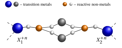
Figure 1: Sketch of a spin-one dimeric magnetic molecule with non-trivial exchange bridge. The identical spin-one ions $X^{+n}_{i}$, with $i=1,2$ and $n\in\mathbb{N}$, are colored in blue, where the letter “$X$” refers to magnetic transition metals. The remaining transition metals (dark-gray balls) belonging to the bridging complex are effectively non-magnetic.

V.1 State functions and energy levels

Let $N$ be the total number of all electrons in the considered dimer described by Hamiltonian (10). Since $N$ is an even number and we consider one exchange bridge, the total number of orbitals will be given by $n=N/2+2$, where we have $n-4$ core and $4$ active molecular orbitals. Respectively, the index $\tau$ will be unique and given by $\tau=(n-3,n-2),(n-1,n)$. We assume the energy of orbitals $(n-1,n)$ to be slightly higher than the energy of the pair $(n-3,n-2)$ yet the orbitals within each pair are energetically equal. Therefore, the number of all functions in (III.3) will depend on the values of $v_{\tau,s_{n-3,n-2},s_{n-1,n},s}$, where the considered system is characterized by the spin coupling set $\{s_{n-3,n-2},s_{n-1,n},s,m\}$.

With respect to the total spin quantum number we distinguish three levels $s=0,1,2$. The singlet level consists of two spin-multiplets $\{0,0,0,0\}$ and $\{1,1,0,0\}$. Accounting for all energetically distinct spin-orbitals configurations, described by the functions (III.3), the multiplet $\{0,0,0,0\}$ appears as $9$-fold degenerate. Thus, we have $v_{\tau,0,0,0}=1,2\ldots,9$ and $v_{\tau,1,1,0}=1$, respectively. In the case of constructive interference between double occupied $(n-3)$-th and $(n-2)$-th molecular orbitals, from all nine multiplets $\{0,0,0,0\}$, we distinguish three states

$$\Psi^{\tau,1}_{0,0,0,0}(\mathbf{r}_{1},\ldots,\mathbf{r}_{N})= \sum_{P_{\mathbf{r}_{1}\ldots\mathbf{r}_{N}}}\!\!\!\frac{c_{\mathbf{r}_{1},\ldots,\mathbf{r}_{N}}}{\sqrt{2^{-\frac{N}{2}}N!}}\prod_{i=1}^{\frac{N}{2}-2}\Phi^{i}_{0,0}(\mathbf{r}_{2i-1},\mathbf{r}_{2i})$$

$$\times\Phi^{n-3,n-2}_{0,0}(\mathbf{r}_{N-3},\mathbf{r}_{N-2})\Phi^{n-1,n}_{0,0}(\mathbf{r}_{N-1},\mathbf{r}_{N}),$$ (43a)

$$\Psi^{\tau,2}_{0,0,0,0}(\mathbf{r}_{1},\ldots,\mathbf{r}_{N})= \sum_{P_{\mathbf{r}_{1}\ldots\mathbf{r}_{N}}}\!\!\!\frac{c_{\mathbf{r}_{1},\ldots,\mathbf{r}_{N}}}{\sqrt{2^{-\frac{N}{2}}N!}}\prod_{i=1}^{\frac{N}{2}-2}\Phi^{i}_{0,0}(\mathbf{r}_{2i-1},\mathbf{r}_{2i})$$

$$\times\Phi^{n-3,n-2}_{0,0}(\mathbf{r}_{N-3},\mathbf{r}_{N-2})\varPhi^{n-1,n}_{0,0}(\mathbf{r}_{N-1},\mathbf{r}_{N}),$$ (43b)

$$\Psi^{\tau,3}_{0,0,0,0}(\mathbf{r}_{1},\ldots,\mathbf{r}_{N})= \sum_{P_{\mathbf{r}_{1}\ldots\mathbf{r}_{N}}}\!\!\!\frac{c_{\mathbf{r}_{1},\ldots,\mathbf{r}_{N}}}{\sqrt{2^{-\frac{N}{2}}N!}}\prod_{i=1}^{\frac{N}{2}-2}\Phi^{i}_{0,0}(\mathbf{r}_{2i-1},\mathbf{r}_{2i})$$

$$\times\Phi^{n-3,n-2}_{0,0}(\mathbf{r}_{N-3},\mathbf{r}_{N-2})\Psi^{n-1,n}_{0,0}(\mathbf{r}_{N-1},\mathbf{r}_{N}),$$ (43c)

where the coefficients $c_{\mathbf{r}_{1},\ldots,\mathbf{r}_{N}}$ account for the antisymmetry of the functions and the sum runs over the permutation of all electrons occupying orbitals of different energy. Here, the permutation $\Phi^{n}_{0,0}(\mathbf{r}_{i},\mathbf{r}_{j})\to\Phi^{n}_{0,0}(\mathbf{r}_{j},\mathbf{r}_{i})$ is not included, see (A.2). Further, according to (4) and in terms of up and down notations the functions in the summands are given by

$$\Phi^{n}_{0,0}(\mathbf{r}_{i},\mathbf{r}_{j})=\frac{1}{\sqrt{2}}\big{(}\phi_{n,\uparrow}(\mathbf{r}_{i})\phi_{n,\downarrow}(\mathbf{r}_{j})-\phi_{n,\downarrow}(\mathbf{r}_{i})\phi_{n,\uparrow}(\mathbf{r}_{j})\big{)},$$

where $s_{n}=0$, $m_{n}=0$,

$$\Phi^{n^{\prime},n}_{0,0}(\mathbf{r}_{i},\mathbf{r}_{j})= \frac{1}{\sqrt{4}}\Big{(}\phi_{n^{\prime},\uparrow}(\mathbf{r}_{i})\phi_{n^{\prime},\downarrow}(\mathbf{r}_{j})$$

$$-\phi_{n^{\prime},\downarrow}(\mathbf{r}_{i})\phi_{n^{\prime},\uparrow}(\mathbf{r}_{j})$$

$$+\phi_{n,\uparrow}(\mathbf{r}_{i})\phi_{n,\downarrow}(\mathbf{r}_{j})-\phi_{n,\downarrow}(\mathbf{r}_{i})\phi_{n,\uparrow}(\mathbf{r}_{j})\Big{)},$$

with $s_{n^{\prime},n}=0$ and $m_{n^{\prime},n}=0$ the constructive superposition between doubly occupied $n^{\prime}$-th and $n$-th orbitals,

$$\varPhi^{n^{\prime},n}_{0,0}(\mathbf{r}_{i},\mathbf{r}_{j})= \frac{1}{\sqrt{4}}\Big{(}\phi_{n^{\prime},\uparrow}(\mathbf{r}_{i})\phi_{n^{\prime},\downarrow}(\mathbf{r}_{j})$$

$$-\phi_{n^{\prime},\downarrow}(\mathbf{r}_{i})\phi_{n^{\prime},\uparrow}(\mathbf{r}_{j})$$

$$-\phi_{n,\uparrow}(\mathbf{r}_{i})\phi_{n,\downarrow}(\mathbf{r}_{j})+\phi_{n,\downarrow}(\mathbf{r}_{i})\phi_{n,\uparrow}(\mathbf{r}_{j})\Big{)},$$

is the destructive counterpart and

$$\Psi^{n^{\prime},n}_{0,0}(\mathbf{r}_{i},\mathbf{r}_{j})= \frac{1}{\sqrt{4}}\Big{(}\phi_{n^{\prime},\uparrow}(\mathbf{r}_{i})\phi_{n,\downarrow}(\mathbf{r}_{j})-\phi_{n^{\prime},\downarrow}(\mathbf{r}_{i})\phi_{n,\uparrow}(\mathbf{r}_{j})$$

$$+\phi_{n,\uparrow}(\mathbf{r}_{i})\phi_{n^{\prime},\downarrow}(\mathbf{r}_{j})-\phi_{n,\downarrow}(\mathbf{r}_{i})\phi_{n^{\prime},\uparrow}(\mathbf{r}_{j})\Big{)},$$

corresponds to the same local singlet with half-filled $n^{\prime}$-th and $n$-th orbitals.

The triplet level is build up from three spin-multiplets, $\{0,1,1,m\}$, $\{1,0,1,m\}$ and $\{1,1,1,m\}$, where $v_{\tau,0,1,1}=1,2,3$, $v_{\tau,1,0,1}=1,2,3$ and $v_{\tau,1,1,1}=1$, respectively. As an example, consider the triplet $\{0,1,1,+1\}$ with $s_{n-3,n-2}=0$, $s_{n-1,n}\equiv s=1$ and $m_{n-1,n}\equiv m=+1$. Thus, we have

$$\Psi^{\tau,1}_{0,1,1,+1}(\mathbf{r}_{1},\ldots,\mathbf{r}_{N})= \sum_{P_{\mathbf{r}_{1}\ldots\mathbf{r}_{N}}}\!\!\!\frac{c_{\mathbf{r}_{1},\ldots,\mathbf{r}_{N}}}{\sqrt{2^{-\frac{N}{2}}N!}}\prod_{i=1}^{\frac{N}{2}-2}\Phi^{i}_{0,0}(\mathbf{r}_{2i-1},\mathbf{r}_{2i})$$

$$\!\!\times\!\!\Phi^{n-3,n-2}_{0,0}(\mathbf{r}_{N-3},\mathbf{r}_{N-2})\Psi^{n-1,n}_{1,+1}(\mathbf{r}_{N-1},\mathbf{r}_{N}),$$ (44)

$$\Psi^{\tau,2}_{0,1,1,+1}(\mathbf{r}_{1},\ldots,\mathbf{r}_{N})= \sum_{P_{\mathbf{r}_{1}\ldots\mathbf{r}_{N}}}\!\!\!\frac{c_{\mathbf{r}_{1},\ldots,\mathbf{r}_{N}}}{\sqrt{2^{-\frac{N}{2}}N!}}\prod_{i=1}^{\frac{N}{2}-2}\Phi^{i}_{0,0}(\mathbf{r}_{2i-1},\mathbf{r}_{2i})$$

$$\!\!\times\!\!\varPhi^{n-3,n-2}_{0,0}(\mathbf{r}_{N-3},\mathbf{r}_{N-2})\Psi^{n-1,n}_{1,+1}(\mathbf{r}_{N-1},\mathbf{r}_{N}),$$

$$\Psi^{\tau,3}_{0,1,1,+1}(\mathbf{r}_{1},\ldots,\mathbf{r}_{N})= \sum_{P_{\mathbf{r}_{1}\ldots\mathbf{r}_{N}}}\!\!\!\frac{c_{\mathbf{r}_{1},\ldots,\mathbf{r}_{N}}}{\sqrt{2^{-\frac{N}{2}}N!}}\prod_{i=1}^{\frac{N}{2}-2}\Phi^{i}_{0,0}(\mathbf{r}_{2i-1},\mathbf{r}_{2i})$$

$$\!\!\!\times\!\!\Psi^{n-3,n-2}_{0,0}(\mathbf{r}_{N-3},\mathbf{r}_{N-2})\Psi^{n-1,n}_{1,+1}(\mathbf{r}_{N-1},\mathbf{r}_{N}),$$

where

$$\Psi^{n^{\prime},n}_{1,+1}(\mathbf{r}_{i},\mathbf{r}_{j})= \frac{1}{\sqrt{2}}\Big{(}\phi_{n^{\prime},\uparrow}(\mathbf{r}_{i})\phi_{n,\uparrow}(\mathbf{r}_{j})-\phi_{n,\uparrow}(\mathbf{r}_{i})\phi_{n^{\prime},\uparrow}(\mathbf{r}_{j})\Big{)}.$$

The quintet level, $\{1,1,2,m\}$, is unique and it is non-degenerate regarding the existing spin-orbitals configurations. As a result, the index $v_{\tau,1,1,2}=1$ and the state of maximal spin magnetic moment $m=2$, reads

$$\Psi^{\tau,1}_{1,1,2,+2}(\mathbf{r}_{1},\ldots,\mathbf{r}_{N})= \sum_{P_{\mathbf{r}_{1}\ldots\mathbf{r}_{N}}}\!\!\!\frac{c_{\mathbf{r}_{1},\ldots,\mathbf{r}_{N}}}{\sqrt{2^{-\frac{N}{2}}N!}}\prod_{i=1}^{\frac{N}{2}-2}\Phi^{i}_{0,0}(\mathbf{r}_{2i-1},\mathbf{r}_{2i})$$

$$\!\!\!\times\!\!\Psi^{n-3,n-2}_{1,+1}(\mathbf{r}_{N-3},\mathbf{r}_{N-2})\Psi^{n-1,n}_{1,+1}(\mathbf{r}_{N-1},\mathbf{r}_{N}).$$

Constructing the effective matrix elements with the aid of (III.3) and accounting for the integrals given in Sec. III.4, with respect to the singlet states (43), we get

$$\big{\langle}\Psi^{\tau,1}_{0,0,0,0}\big{\rvert}\hat{H}_{\mathrm{eff}}\big{\lvert}\Psi^{\tau,1}_{0,0,0,0}\big{\rangle}=U_{\tau}+D_{\tau},$$ (45a)

$$\big{\langle}\Psi^{\tau,2}_{0,0,0,0}\big{\rvert}\hat{H}_{\mathrm{eff}}\big{\lvert}\Psi^{\tau,2}_{0,0,0,0}\big{\rangle}=U_{\tau}-D_{\tau},$$ (45b)

$$\big{\langle}\Psi^{\tau,3}_{0,0,0,0}\big{\rvert}\hat{H}_{\mathrm{eff}}\big{\lvert}\Psi^{\tau,3}_{0,0,0,0}\big{\rangle}=V_{\tau}+D_{\tau},$$ (45c)

respectively. Furthermore, using the triplet state (V.1), for $m=0,\pm 1$ we have

$$\big{\langle}\Psi^{\tau,1}_{0,1,1,m}\big{\rvert}\hat{H}_{\mathrm{eff}}\big{\lvert}\Psi^{\tau,1}_{0,1,1,m}\big{\rangle}= V_{\tau}-D_{\tau}-\mu_{\mathrm{B}}Bm\sum^{N}_{i=1}\langle g^{\alpha}_{i}\rangle^{(1)}_{\tau,0,1,1}.$$ (46)

Working with (45) and (46), one has to bear in mind that (22) is rewritten according to the considered case and for example $U_{\tau}$ is a function of the single orbital integrals $U_{n-3},U_{n-2},U_{n-1}$ and $U_{n}$.

Computing the eigenvalues in (19) we obtain $9$ energy levels associated to the total singlet $s=0$, where $n_{\tau,0,0,0}=1,2,\ldots,9$ and $n_{\tau,1,1,0}=1$. Further, we get $21$ triplet levels corresponding to the indexes $n_{\tau,0,1,1}=1,2,3$, $n_{\tau,1,0,1}=1,2,3$ and $n_{\tau,1,1,1}=1$ for all $m=0,\pm 1$. As an example, since the triplet $\{1,1,1,m\}$ is unique, from (20) we get $\lvert\Omega^{\tau,1}_{1,1,1,m}\rangle\equiv\lvert\Psi^{\tau,1}_{1,1,1,m}\rangle$. Consequently, the corresponding eigenvalues from (19a) and (19b) read

$$E^{\mathrm{f},(1)}_{\tau,1,1,1,m}=V^{\prime}_{\tau}-D^{\prime}_{\tau}$$

and

$$\mathcal{E}^{(1)}_{\tau,1,1,1,m}=-\mu_{\mathrm{B}}Bm\sum^{N}_{i=1}\langle g^{\alpha}_{i}\rangle^{(1)}_{\tau,1,1,1},$$

respectively, where due to the different spin configuration related to the orbitals $n-3$ and $n-2$, we have $V^{\prime}_{\tau}\neq V_{\tau}$ and $D^{\prime}_{\tau}\neq D_{\tau}$.

The quintet level consists of five energy levels with $n_{\tau,1,1,2}=1$ and $m=0,\pm 1,\pm 2$.

V.2 Energy spectrum

Constructing the effective total spin space we take into account (21). Since index $\tau$ is unique the sum runs over all values of $n_{\tau,s_{n-3,n-2},s_{n-1,n},s}$ for each spin multiplet $\{s_{n-3,n-2},s_{n-1,n},s,m\}$. Thus, for all $m=0,\pm 1$, the triplet states read

$$\lvert 1,m\rangle= c^{(1)}_{1,1,1,m}\big{\lvert}\Omega^{\tau,n_{\tau,1,1,1}}_{1,1,1,m}\big{\rangle}+\!\!\!\!\sum^{3}_{n_{\tau,0,1,1}=1}c^{(n_{\tau,0,1,1})}_{0,1,1,m}\big{\lvert}\Omega^{\tau,n_{\tau,0,1,1}}_{0,1,1,m}\big{\rangle}$$

$$+\sum^{3}_{n_{\tau,1,0,1}=1}c^{(n_{\tau,1,0,1})}_{1,0,1,m}\big{\lvert}\Omega^{\tau,n_{\tau,1,0,1}}_{1,0,1,m}\big{\rangle},$$

where according to (28) the corresponding triplet energy is given by

$$E^{\mathrm{f}}_{1,m}= \big{|}c^{(1)}_{1,1,1,m}\big{|}^{2}\rho^{(1)}_{1,1,1,m}\varSigma^{\mathrm{f},(1)}_{1,1,1,m}$$

$$+\sum^{3}_{n_{\tau,0,1,1}=1}\big{|}c^{(n_{\tau,0,1,1})}_{0,1,1,m}\big{|}^{2}\rho^{(n_{\tau,0,1,1})}_{0,1,1,m}\varSigma^{\mathrm{f},(n_{\tau,0,1,1})}_{0,1,1,m}$$

$$+\sum^{3}_{n_{\tau,1,0,1}=1}\big{|}c^{(n_{\tau,1,0,1})}_{1,0,1,m}\big{|}^{2}\rho^{(n_{\tau,1,0,1})}_{1,0,1,m}\varSigma^{\mathrm{f},(n_{\tau,1,0,1})}_{1,0,1,m}.$$ (47a)

For the sake of clarity we write down the singlet energy,

$$E^{\mathrm{f}}_{0,0}= \big{|}c^{(1)}_{1,1,0,0}\big{|}^{2}\rho^{(1)}_{1,1,0,0}\varSigma^{\mathrm{f},(1)}_{1,1,0,0}$$

$$+\sum^{9}_{n_{\tau,0,0,0}=1}\big{|}c^{(n_{\tau,0,0,0})}_{0,0,0,0}\big{|}^{2}\rho^{(n_{\tau,0,0,0})}_{0,0,0,0}\varSigma^{\mathrm{f},(n_{\tau,0,0,0})}_{0,0,0,0}.$$ (47b)

The quintet level is unique. For all $m$, $c^{(1)}_{1,1,2,m}=1$ and hence

$$E^{\mathrm{f}}_{2,m}=\rho^{(1)}_{1,1,2,m}\varSigma^{\mathrm{f},(1)}_{1,1,2,m}.$$ (47c)

In the case $|\mathbf{B}|=0$, we have $E^{\mathrm{f}}_{s,m}\to E_{s,m}$.

V.3 Magnetic transitions

In the absence of an external magnetic field and at $T\to 0$ the dimer is in its ground state with energy $E_{0,0}$. The first excited level is the triplet with energy $E_{1,m}$, where $m=0,\pm 1$.

Assume measuring the dimer’s magnetic spectrum, we perform an inelastic neutron scattering experiment. Applying the corresponding selection rules under the considered spin coupling scheme, we take into account that for the allowed energy transitions the local spin quantum numbers $s_{n-3,n-2}$ and $s_{n-1,n}$ cannot be simultaneously changed. Accordingly, with respect to the quantum probabilities in (47) and (47), the applied variational method predicts one broadened low-temperature peak in the magnetic spectrum, centered at $E_{1,\Delta m}=E_{1,m}-E_{0,0}$. In particular, the obtained peak will be a product of three slightly energetically different magnetic excitations. One associated to the energy transition with $\Delta s_{n-3,n-2}=0$, $\Delta s_{n-1,n}=0$ and $\Delta s=1$, a second with $\Delta s_{n-3,n-2}=0$, $\Delta s_{n-1,n}=1$, $\Delta s=1$ and a third corresponding to the energy transition for which $\Delta s_{n-3,n-2}=1$, $\Delta s_{n-1,n}=0$, $\Delta s=1$. Thus, depending on the difference in energies of both orbital pairs $(n-3,n-2)$ and $(n-1,n)$ we may expect splitting of the peak.

Theoretically, a high-temperature magnetic transition is also allowed. The center of the corresponding peak will be characterized by the energy $E_{1,\Delta m}=E_{2,m^{\prime}}-E_{1,m}$, for all $m^{\prime}=0,\pm 1,\pm 2$. However, due to the higher temperature, features like broadening and splitting may not be pronounced.

Henceforth, we assume that for $T\to 0$ the probability for observing the transition with $\Delta s_{n-3,n-2}=0$, $\Delta s_{n-1,n}=0$ and $\Delta s=1$ is negligible and hence the low temperature peak is build of two different by intensity peaks, the first centered at

$$E^{(1)}_{1,\Delta m}= \sum^{3}_{n_{\tau,0,1,1}=1}\big{|}c^{(n_{\tau,0,1,1})}_{0,1,1,m}\big{|}^{2}\rho^{(n_{\tau,0,1,1})}_{0,1,1,m}\varSigma^{(n_{\tau,0,1,1})}_{0,1,1,m}$$

$$-\sum^{9}_{n_{\tau,0,0,0}=1}\big{|}c^{(n_{\tau,0,0,0})}_{0,0,0,0}\big{|}^{2}\rho^{(n_{\tau,0,0,0})}_{0,0,0,0}\varSigma^{(n_{\tau,0,0,0})}_{0,0,0,0}$$ (48a)

and the second at

$$E^{(2)}_{1,\Delta m}= \sum^{3}_{n_{\tau,1,0,1}=1}\big{|}c^{(n_{\tau,1,0,1})}_{1,0,1,m}\big{|}^{2}\rho^{(n_{\tau,1,0,1})}_{1,0,1,m}\varSigma^{(n_{\tau,1,0,1})}_{1,0,1,m}$$

$$-\sum^{9}_{n_{\tau,0,0,0}=1}\big{|}c^{(n_{\tau,0,0,0})}_{0,0,0,0}\big{|}^{2}\rho^{(n_{\tau,0,0,0})}_{0,0,0,0}\varSigma^{(n_{\tau,0,0,0})}_{0,0,0,0},$$ (48b)

where $$E^{(2)}_{1,\Delta m}>E^{(1)}_{1,\Delta m} \Delta m=m n_{\tau,0,1,1},n_{\tau,1,0,1}=1,2,3 T>0$$ and . Furthermore, let for all and , we have

$$\rho^{(1)}_{1,1,1,m}\gg\rho^{(n_{\tau,0,1,1})}_{0,1,1,m},\rho^{(n_{\tau,1,0,1})}_{1,0,1,m},$$

whereat the probability of observing a high-temperature magnetic excitation is related only to the transition with energy

$$E^{(3)}_{1,\Delta m}=\rho^{(1)}_{1,1,2,m^{\prime}}\varSigma^{(1)}_{1,1,2,m^{\prime}}-\big{|}c^{(1)}_{1,1,1,m}\big{|}^{2}\rho^{(1)}_{1,1,1,m}\varSigma^{(1)}_{1,1,1,m},$$ (48c)

for all $$\Delta m$$.

In addition, we imply that for each magnetic center the total effective $g$-factor in (42) is taken within the low-field limit, such that $c^{(n_{\tau,s_{\tau},s})}_{\tau,s_{\tau},s,m}\simeq c^{(n_{\tau,s_{\tau},s})}_{\tau,s_{\tau},s,m^{\prime}}$ and $\rho^{(n_{\tau,s_{\tau},s})}_{\tau,s_{\tau},s,m}\simeq\rho^{(n_{\tau,s_{\tau},s})}_{\tau,s_{\tau},s,m^{\prime}}$, where $m\neq m^{\prime}$.

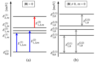
Figure 2: Energy spectrum of the considered spin-one dimer: (a) in the absence of magnetic field; (b) the energy levels of the non-magnetic states in the presence of magnetic field. The blue and red arrows depict the low-temperature and high-temperature magnetic transitions, respectively, see (51) and (52). The gray arrows show the energy level’s shifting due to the indirect action of $\mathbf{B}$, indicated by the “$h$-field” parameters in (55).

V.4 The dimer spin-sigma Hamiltonian

In order to construct an adequate energy spectrum that capture the physics behind the obtained variational energy spectrum discussed in Sec. V.2, account for the transitions (48) and simplify the computation of any relevant magnetic observables, we consider the spin-sigma Hamiltonian (31), that reads

$$\hat{\mathcal{H}}=J\big{(}\hat{\boldsymbol{\sigma}}_{1}\cdot\hat{\mathbf{s}}_{2}+\hat{\boldsymbol{\sigma}}_{2}\cdot\hat{\mathbf{s}}_{1}\big{)}-\mu_{\mathrm{B}}B\Big{(}\hat{S}^{z}_{1}+\hat{S}^{z}_{2}\Big{)},$$

where $J_{12}=J_{21}=J$ and we select the $z$ axis as a quantization axis. Both $\boldsymbol{\sigma}$-operators share the same coefficients $a_{s,n_{s}}=h_{s}c_{s,n_{s}}$ and hence obey (38), such that $|s_{2}+s_{1}|\geq s\geq|s_{2}-s_{1}|$ is the pair’s total spin quantum number and $s_{i}$ is the spin quantum number of the $i$-th effective magnetic center. Further, since both magnetic ions are indistinguishable and the $g$-factor is calculated within a low-temperature and low-field regime, we have $\mathrm{g}^{z}_{1,s,m}=\mathrm{g}^{z}_{2,s,m}\to\mathrm{g}^{z}_{s}$. Therefore, using (40) and (41), we get

$$\hat{\mathcal{H}}\lvert s,m\rangle_{n_{s}}=\mathcal{E}^{\mathrm{f},(n_{s})}_{s,m}\lvert s,m\rangle_{n_{s}},$$

where

$$\mathcal{E}^{\mathrm{f},(n_{s})}_{s,m}= \frac{Jh_{s}c_{s,n_{s}}}{2}\big{(}s(s+1)-s_{1}(s_{1}+1)-s_{2}(s_{2}+1)\big{)}$$

$$-m\mu_{\mathrm{B}}\mathrm{g}^{z}_{s}B.$$ (49)

Since all transitions given in (48) are related to the triplet state and the quintet state is unique, it follows that $n_{0}=1$, $n_{2}=1$ and $n_{1}=1,2,3$, with $c_{0,1}=1$ and $c_{2,1}=1$. Hence, we are left with three field parameters $\{h_{s}\}^{3}_{s=1}$ and three spectroscopic parameters $\{c_{1,n_{1}}\}^{3}_{n_{1}=1}$. The spectrum (V.4) consists of fifteen energy levels

$$\begin{array}[]{ll}\mathcal{E}^{\mathrm{f},(1)}_{2,m}=Jh_{2}-m\mu_{\mathrm{B}}\mathrm{g}^{z}_{2}B,&\mathcal{E}^{\mathrm{f},(3)}_{1,m}=-Jh_{1}c_{1,3}-m\mu_{\mathrm{B}}\mathrm{g}^{z}_{1}B,\\[7.11317pt] \mathcal{E}^{\mathrm{f},(1)}_{1,m}=-Jh_{1}c_{1,1}-m\mu_{\mathrm{B}}\mathrm{g}^{z}_{1}B,&\mathcal{E}^{\mathrm{f},(1)}_{0,0}=-2Jh_{0},\\[7.11317pt] \mathcal{E}^{\mathrm{f},(2)}_{1,m}=-Jh_{1}c_{1,2}-m\mu_{\mathrm{B}}\mathrm{g}^{z}_{1}B.&{}\end{array}$$ (50)

In the absence of external magnetic field $h_{s}=1$, for all $s$ and therefore $\mathcal{E}^{\mathrm{f},(1)}_{1,m}\to\mathcal{E}^{(1)}_{1,m}$, where $\mathcal{E}^{(1)}_{1,m}=-Jc_{1,1}$.

According to (48), we observe two low-temperature magnetic excitations with energies

$$\mathcal{E}^{(1)}_{1,m}-\mathcal{E}^{(1)}_{0,0}=E^{(1)}_{1,\Delta m},\qquad\mathcal{E}^{(2)}_{1,m}-\mathcal{E}^{(1)}_{0,0}=E^{(2)}_{1,\Delta m}$$ (51)

and a high-temperature one, with energy

$$\mathcal{E}^{(1)}_{2,m}-\mathcal{E}^{(3)}_{1,m^{\prime}}=E^{(3)}_{1,\Delta m}.$$ (52)

Determining the spectroscopic parameters, from (51) and (52), we obtain

$$J=E^{(1)}_{1,\Delta m},\quad c_{1,1}=1,\quad c_{1,2}=2-\frac{E^{(2)}_{1,\Delta m}}{E^{(1)}_{1,\Delta m}}$$ (53)

and

$$c_{1,3}=\frac{E^{(3)}_{1,\Delta m}}{E^{(1)}_{1,\Delta m}}-1,$$ (54)

respectively. The energy spectrum with all transitions are depicted on Fig. 2 (a).

Obtaining the expressions for the “$h$–field” parameters, we take into account the energy levels corresponding only to the non-magnetic states, i.e. for $m=0$. Thus, in addition to (51) and (52), we have

$$\mathcal{E}^{\mathrm{f},(1)}_{1,0}-\mathcal{E}^{\mathrm{f},(1)}_{0,0}=E^{\mathrm{f},(1)}_{1,0},\qquad\mathcal{E}^{\mathrm{f},(2)}_{1,0}-\mathcal{E}^{\mathrm{f},(1)}_{0,0}=E^{(2)}_{1,0}$$

and

$$\mathcal{E}^{\mathrm{f},(1)}_{2,0}-\mathcal{E}^{\mathrm{f},(3)}_{1,0}=E^{\mathrm{f},(3)}_{1,0},$$

respectively. As a result, we get

$$h_{0}=\frac{E^{\mathrm{f},(1)}_{1,0}+E^{\mathrm{f},(2)}_{1,0}}{4E^{(1)}_{1,\Delta m}}+\frac{1}{4}\left(3-\frac{E^{(2)}_{1,\Delta m}}{E^{(1)}_{1,\Delta m}}\right)\frac{E^{\mathrm{f},(1)}_{1,0}-E^{\mathrm{f},(2)}_{1,0}}{E^{(1)}_{1,\Delta m}-E^{(2)}_{1,\Delta m}},$$ (55a)

$$h_{1}=\frac{E^{\mathrm{f},(1)}_{1,0}-E^{\mathrm{f},(2)}_{1,0}}{E^{(1)}_{1,\Delta m}-E^{(2)}_{1,\Delta m}}$$ (55b)

and

$$h_{2}=\frac{E^{\mathrm{f},(3)}_{1,0}}{E^{(1)}_{1,\Delta m}}-\left(\frac{E^{(3)}_{1,\Delta m}}{E^{(1)}_{1,\Delta m}}-1\right)\frac{E^{\mathrm{f},(1)}_{1,0}-E^{\mathrm{f},(2)}_{1,0}}{E^{(1)}_{1,\Delta m}-E^{(2)}_{1,\Delta m}}.$$ (55c)

An illustration of how the external magnetic field may shift the non-magnetic energy levels due to the contribution of all diamagnetic and paramagnetic terms (12) is shown on Fig. 2 (b). This effect is considered as the main reason for the observed broadening of the magnetization steps of the molecular magnet Ni₄Mo₁₂, discussed in [59]

VI Conclusion

We present a detailed discussion on the theoretical framework recently used to study the magnetic properties of the Cu based spin-trimeric compounds [57] and Ni₄Mo₁₂ molecular magnet [58, 59]. The introduced method, see Sec. III, is based on the molecular orbital theory and follows closely the multi-configurational self-consistent field approach. The method produces a generalized energy spectrum that accounts for all distinct in energy spin-orbital configurations and hence nonhomogeneous electrons’ distributions that may result form the spatial structure of the studied magnetic unit. Moreover, individual orbitals have but minor contributions due to the delocalization of electrons, such that the associated anisotropy effects vanish. Thus, the obtained energy sequence predicts the existence of multiple possible magnetic excitations that are not related to energy transitions from the fine or hyper-fine structure in a zero-field approximation, but rather result from the excitation of electron pairs of different distributions. Broadened steps and a high-field saturation in magnetization is yet another possible feature.

Based on all predictions made within the framework of our method, in Sec. IV we propose a spin-like Hamiltonian with an appropriately selected parametrization scheme that captures the relevant magnetic features. In particular, the spin Hamiltonian includes two class of parameters, spectroscopic and field parameters, see (40a). The “$c$–spectroscopic” parameters account for all magnetic excitations contained in the variational energy spectrum and they can be fitted according to the relevant experimentally observed magnetic spectra. On the other hand, the “$h$–field” parameters address the shifting of all energy levels due to the indirect action of an externally applied magnetic field, see Sec. III.4. Their value can be fixed from the magnetization and magnetic susceptibility measurements.

As an example, for the application of the introduced method and spin-sigma model, we consider a fictive spin-one dimer molecular magnet with non-trivial bridging structure, see Sec. V. We derive the explicit expressions of the variational state functions (III.3), construct the energy spectrum (28) and discuss all allowed magnetic excitations associated to the transitions (III.5). Further, we introduce the dimer’s Hamiltonian (31) and the corresponding eigenvalues. In other words, we compute the “$c$–spectroscopic” and “$h$–field” parameters and hence show how the spin-sigma energy spectrum allows the derivation of the main features of that relevant to the variational approach.

Although the spin-like Hamiltonian (31) includes only a bilinear exchange interaction term (30a), it may describe reasonably well the magnetism in larger and more complex molecular magnets with $n$d or $n$f metal centers. However, the application of the underlying method proposed is Sec. III, remains restricted to specific variety of compounds in which the electrons are not localized around the magnetic ions and do not belong to a conduction band. Therefore, additional terms that account for any perturbation parameter addressing spin-orbital anisotropy would be inappropriate.

*

Appendix A

A.1 Generalized momentum

Since for all $\alpha$ and $i$ the operators $\hat{A}_{\alpha}(\mathbf{r}_{i})$ and $\hat{p}^{\alpha}_{i}$ given in Section III.1 commute, the $i$-th electron’s generalized momentum operator reads

$$\hat{\mathbf{P}}^{2}_{i}=\hat{\mathbf{p}}^{2}_{i}-2e\hat{\mathbf{A}}_{ext}(\mathbf{r}_{i})\cdot\hat{\mathbf{p}}_{i}+2e\!\!\!\!\sum_{j|_{j\neq i}}\hat{\mathbf{A}}(\mathbf{r}_{ij})\cdot\hat{\mathbf{p}}_{i}+e^{2}\hat{\mathbf{A}}^{2}(\mathbf{r}_{i}),$$

where

$$\hat{\mathbf{A}}^{2}(\mathbf{r}_{i})=\hat{\mathbf{A}}^{2}_{ext}(\mathbf{r}_{i})+2\sum_{j|_{j\neq i}}\hat{\mathbf{A}}_{ext}(\mathbf{r}_{i})\cdot\hat{\mathbf{A}}(\mathbf{r}_{ij})+\left(\sum_{j|_{j\neq i}}\hat{\mathbf{A}}(\mathbf{r}_{ij})\right)^{2}.$$

In terms of (8) we have the diamagnetic term

$$\hat{\mathbf{A}}^{2}_{ext}(\mathbf{r}_{i})=\frac{\mathbf{B}^{2}\mathbf{r}^{2}_{i}}{4},$$ (56a)

the paramagnetic terms

$$\hat{\mathbf{A}}_{ext}(\mathbf{r}_{i})\cdot\hat{\mathbf{p}}_{i}=\frac{\hbar}{2}\hat{\boldsymbol{l}}_{i}\cdot\mathbf{B},$$ (56b)

$$\hat{\mathbf{A}}(\mathbf{r}_{ij})\cdot\hat{\mathbf{p}}_{i}=\frac{\mu_{0}\mu_{\mathrm{B}}\hbar}{4\pi^{2}\langle r_{ij}\rangle^{3}}\left(\hat{\boldsymbol{l}}_{i}\cdot\hat{\boldsymbol{l}}_{j}+g_{s}\hat{\boldsymbol{l}}_{i}\cdot\hat{\boldsymbol{s}}_{j}\right),$$ (56c)

$$\hat{\mathbf{A}}_{ext}(\mathbf{r}_{i})\cdot\hat{\mathbf{A}}(\mathbf{r}_{ij})= \frac{\mu_{0}\mu_{\mathrm{B}}}{8\pi^{2}\langle r_{ij}\rangle^{3}}\bigg{[}\left(\mathbf{r}_{ij}\cdot\mathbf{B}\right)\left(\mathbf{r}_{i}\cdot\hat{\boldsymbol{l}}_{j}\right)$$

$$-\left(\mathbf{r}_{i}\cdot\mathbf{r}_{ij}\right)\left(\hat{\boldsymbol{l}}_{j}\cdot\mathbf{B}\right)\bigg{]}$$

$$+\frac{\mu_{0}\mu_{\mathrm{B}}g_{s}}{8\pi^{2}\langle r_{ij}\rangle^{3}}\bigg{[}\left(\mathbf{r}_{ij}\cdot\mathbf{B}\right)\left(\mathbf{r}_{i}\cdot\hat{\boldsymbol{s}}_{j}\right)$$

$$-\left(\mathbf{r}_{i}\cdot\mathbf{r}_{ij}\right)\left(\hat{\boldsymbol{s}}_{j}\cdot\mathbf{B}\right)\bigg{]}$$ (56d)

and

$$\left(\sum_{j|_{j\neq i}}\hat{\mathbf{A}}(\mathbf{r}_{ij})\right)^{2}= \frac{\mu^{2}_{0}\mu^{2}_{\mathrm{B}}}{16\pi^{4}}\sum_{j|_{j\neq i}}\Bigg{(}\frac{\mathbf{r}^{2}_{ij}\hat{\boldsymbol{l}}^{2}_{j}}{\langle r_{ij}\rangle^{6}}+\sum_{k|_{k\neq j}}\!\!\left(\langle r_{ij}\rangle\langle r_{ik}\rangle\right)^{-3}$$

$$\times\big{[}(\mathbf{r}_{ij}\cdot\mathbf{r}_{ik})(\hat{\boldsymbol{l}}_{j}\cdot\hat{\boldsymbol{l}}_{k})-(\mathbf{r}_{ij}\cdot\hat{\boldsymbol{l}}_{k})(\mathbf{r}_{ik}\cdot\hat{\boldsymbol{l}}_{j})\big{]}\Bigg{)}$$

$$+\frac{\mu^{2}_{0}\mu^{2}_{\mathrm{B}}g^{2}_{s}}{16\pi^{4}}\sum_{j|_{j\neq i}}\Bigg{(}\frac{\mathbf{r}^{2}_{ij}\hat{\boldsymbol{s}}^{2}_{j}}{\langle r_{ij}\rangle^{6}}+\!\!\!\!\sum_{k|_{k\neq j}}\!\!\!\left(\langle r_{ij}\rangle\langle r_{ik}\rangle\right)^{-3}$$

$$\times\big{[}(\mathbf{r}_{ij}\cdot\mathbf{r}_{ik})(\hat{\boldsymbol{s}}_{j}\cdot\hat{\boldsymbol{s}}_{k})-(\mathbf{r}_{ij}\cdot\hat{\boldsymbol{s}}_{k})(\mathbf{r}_{ik}\cdot\hat{\boldsymbol{s}}_{j})\big{]}\Bigg{)}$$

$$+\frac{\mu^{2}_{0}\mu^{2}_{\mathrm{B}}g_{s}}{16\pi^{4}}\sum_{j,k|_{j\neq k\neq i}}\!\!\!\!\!\frac{\big{\{}(\mathbf{r}_{ij}\times\hat{\boldsymbol{l}}_{j})_{\alpha},(\mathbf{r}_{ik}\times\hat{\boldsymbol{s}}_{k})_{\alpha}\big{\}}}{\left(\langle r_{ij}\rangle\langle r_{ik}\rangle\right)^{3}},$$ (57)

where we have the unit vector $\mathbf{n}_{ij}$ defined by $\mathbf{n}_{ij}=\mathbf{r}_{ij}/\langle r_{ij}\rangle$. For $|\mathbf{B}|>0$, in comparison to the terms in (56), the average of the operator in (A.1) can be neglected. Thus, taking into account that $\mu_{\mathrm{B}}=e\hbar/2m_{e}$ within the combination of (56c) and (56) we find it more convenient to define the operators (9) and (9), entering in the expression (9) for the $i$-th electron’s generalized momentum operator.

A.2 Four electrons state

In the case of four electrons, $N=4$, with one core $\phi_{1}$ and two active $\phi_{2}$, $\phi_{3}$ molecular orbitals, the index $\tau=(2,3)$ is unique, the spin quantum number related to the core orbital $s_{1}=0$, $s_{(2,3)}\equiv s$ is the total spin quantum number since the spin pair is unique and hence $v_{\tau,s_{\tau},s}\equiv v_{(2,3),s}$. We have three linear independent combinations with $v_{(2,3),0}=1,2,3$ associated to the singlet level $s=0$ and one corresponding to the triplet level $v_{(2,3),1}=1$. Let us focus on the non-magnetic triplet indicated by $v_{(2,3),1}=1$, $s=1$, $m=0$, with unique coefficient $c^{1}_{2,3}=1$ and given according to (III.3) as follows

$${\Psi^{1,(2,3)}_{1,0}}(\mathbf{r}_{1},\ldots,\mathbf{r}_{4})\equiv \frac{1}{\sqrt{6}}\Big{(}\Phi^{1}_{0,0}(\mathbf{r}_{1},\mathbf{r}_{2})\Psi^{2,3}_{1,0}(\mathbf{r}_{3},\mathbf{r}_{4})$$

$$-\Phi^{1}_{0,0}(\mathbf{r}_{1},\mathbf{r}_{3})\Psi^{2,3}_{1,0}(\mathbf{r}_{2},\mathbf{r}_{4})$$

$$+\Phi^{1}_{0,0}(\mathbf{r}_{1},\mathbf{r}_{4})\Psi^{2,3}_{1,0}(\mathbf{r}_{2},\mathbf{r}_{3})$$

$$+\Phi^{1}_{0,0}(\mathbf{r}_{2},\mathbf{r}_{3})\Psi^{2,3}_{1,0}(\mathbf{r}_{1},\mathbf{r}_{4})$$

$$-\Phi^{1}_{0,0}(\mathbf{r}_{2},\mathbf{r}_{4})\Psi^{2,3}_{1,0}(\mathbf{r}_{1},\mathbf{r}_{3})$$

$$+\Phi^{1}_{0,0}(\mathbf{r}_{3},\mathbf{r}_{4})\Psi^{2,3}_{1,0}(\mathbf{r}_{1},\mathbf{r}_{2})\Big{)},$$ (58)

where with respect to the denotation (4), for $m_{i}\in\{\uparrow,\downarrow\}$, we have

$$\Phi^{1}_{0,0}(\mathbf{r}_{i},\mathbf{r}_{j})=\frac{1}{\sqrt{2}}\big{(}\phi_{1,\uparrow}(\mathbf{r}_{i})\phi_{1,\downarrow}(\mathbf{r}_{j})-\phi_{1,\downarrow}(\mathbf{r}_{i})\phi_{1,\uparrow}(\mathbf{r}_{j})\big{)}$$

and

$$\Psi^{(2,3)}_{1,0}(\mathbf{r}_{i},\mathbf{r}_{j})= \frac{1}{\sqrt{4}}\Big{(}\phi_{2,\uparrow}(\mathbf{r}_{i})\phi_{3,\downarrow}(\mathbf{r}_{j})+\phi_{2,\downarrow}(\mathbf{r}_{i})\phi_{3,\uparrow}(\mathbf{r}_{j})$$

$$-\phi_{3,\uparrow}(\mathbf{r}_{i})\phi_{2,\downarrow}(\mathbf{r}_{j})-\phi_{3,\downarrow}(\mathbf{r}_{i})\phi_{2,\uparrow}(\mathbf{r}_{j})\Big{)}.$$

On the other hand, considering the magnetic triplet $m=+1$, we have

$$\Psi^{(2,3)}_{1,+1}(\mathbf{r}_{i},\mathbf{r}_{j})=\frac{1}{\sqrt{2}}\Big{(}\phi_{2,\uparrow}(\mathbf{r}_{i})\phi_{3,\uparrow}(\mathbf{r}_{j})-\phi_{3,\uparrow}(\mathbf{r}_{i})\phi_{2,\uparrow}(\mathbf{r}_{j})\Big{)}.$$

References

• Gatteschi et al. [2006] D. Gatteschi, R. Sessoli, and J. Villain, Molecular Nanomagnets (Oxford University Press, 2006).
• Winpenny [2011] R. Winpenny, Molecular Cluster Magnets, World Scientific Series in Nanoscience and Nanotechnology, Vol. 3 (WORLD SCIENTIFIC, 2011).
• Bartolomé et al. [2014] J. Bartolomé, F. Luis, and J. F. Fernández, eds., Molecular Magnets: Physics and Applications, NanoScience and Technology (Springer Berlin Heidelberg, Berlin, Heidelberg, 2014).
• Gao [2015] S. Gao, ed., Molecular Nanomagnets and Related Phenomena, Structure and Bonding, Vol. 164 (Springer, Berlin, 2015).
• Coronado [2020] E. Coronado, Molecular magnetism: from chemical design to spin control in molecules, materials and devices, Nat. Rev. Mater. 5, 87 (2020).
• Liu et al. [2019] J. Liu, J. Mrozek, W. K. Myers, G. A. Timco, R. E. Winpenny, B. Kintzel, W. Plass, and A. Ardavan, Electric Field Control of Spins in Molecular Magnets, Phys. Rev. Lett. 122, 037202 (2019).
• Vyaselev et al. [2020] O. M. Vyaselev, N. D. Kushch, E. B. Yagubskii, O. V. Maximova, and A. N. Vasiliev, Spin dynamics in two ReF6-based single-molecule magnets from NMR and ac susceptibility measurements, Phys. Rev. B 101, 134427 (2020).
• Cornia et al. [2020] A. Cornia, A.-L. Barra, V. Bulicanu, R. Clérac, M. Cortijo, E. A. Hillard, R. Galavotti, A. Lunghi, A. Nicolini, M. Rouzières, L. Sorace, and F. Totti, The Origin of Magnetic Anisotropy and Single-Molecule Magnet Behavior in Chromium(II)-Based Extended Metal Atom Chains, Inorg. Chem. 59, 1763 (2020).
• Kowalewska and Szałowski [2020] P. Kowalewska and K. Szałowski, Magnetocaloric properties of V6 molecular magnet, J. Magn. Magn. Mater 496, 165933 (2020).
• Chamati and Romano [2010] H. Chamati and S. Romano, Interaction anisotropy and random impurities - effects on the critical behaviour of ferromagnets, J. Phys.: Conf. Ser. 253, 012011 (2010).
• Chamati [2013] H. Chamati, Theory of Phase Transitions: From Magnets to Biomembranes, Adv. Planar Lipid Bilayers Liposomes 17, 237 (2013).
• Sellmyer et al. [2015] D. J. Sellmyer, B. Balamurugan, B. Das, P. Mukherjee, R. Skomski, and G. C. Hadjipanayis, Novel structures and physics of nanomagnets, J. Appl. Phys. 117, 172609 (2015).
• Sieklucka and Pinkowicz [2017] B. Sieklucka and D. Pinkowicz, eds., Molecular Magnetic Materials: Concepts and Applications (Wiley, Weinheim, 2017).
• Hay et al. [1975] P. J. Hay, J. C. Thibeault, and R. Hoffmann, Orbital interactions in metal dimer complexes, J. Am. Chem. Soc. 97, 4884 (1975).
• Felthouse et al. [1977] T. R. Felthouse, E. J. Laskowski, and D. N. Hendrickson, Magnetic exchange interactions in transition metal dimers. 10. Structural and magnetic characterization of oxalate-bridged, bis(1,1,4,7,7-pentaethyldiethylene triamine)oxalatodicopper tetraphenylborate and related dimers. Effects of nonbridging ligands and counterions on exchange interactions, Inorg. Chem. 16, 1077 (1977).
• Hart et al. [1992] J. R. Hart, A. K. Rappe, S. M. Gorun, and T. H. Upton, Estimation of magnetic exchange coupling constants in bridged dimer complexes, J. Phys. Chem. 96, 6264 (1992).
• Guo and Layfield [2017] F.-S. Guo and R. A. Layfield, Strong direct exchange coupling and single-molecule magnetism in indigo-bridged lanthanide dimers, Chem. Commun. 53, 3130 (2017).
• Gehring et al. [1993] S. Gehring, P. Fleischhauer, H. Paulus, and W. Haase, Ferromagnetic exchange coupling and magneto-structural correlations in mixed-bridged trinuclear copper(II) complexes. Magnetic data and theoretical investigations and crystal structures of two angled CuII3 complexes, Inorg. Chem. 32, 54 (1993).
• Yoon and Solomon [2007] J. Yoon and E. I. Solomon, Electronic structures of exchange coupled trigonal trimeric Cu(II) complexes: Spin frustration, antisymmetric exchange, pseudo-A terms, and their relation to O2 activation in the multicopper oxidases, Coord. Chem. Rev. 251, 379 (2007).
• Ferrer et al. [2012] S. Ferrer, F. Lloret, E. Pardo, J. M. Clemente-Juan, M. Liu-González, and S. García-Granda, Antisymmetric Exchange in Triangular Tricopper(II) Complexes: Correlation among Structural, Magnetic, and Electron Paramagnetic Resonance Parameters, Inorg. Chem. 51, 985 (2012).
• Astheimer and Haase [1986] H. Astheimer and W. Haase, Direct theoretical ab initio calculations in exchange coupled copper (II) dimers: Influence of structural and chemical parameters in modeled copper dimers, J. Chem. Phys. 85, 1427 (1986).
• Charlot et al. [1986] M. F. Charlot, O. Kahn, M. Chaillet, and C. Larrieu, Interaction between copper(II) ions through the azido bridge: concept of spin polarization and ab initio calculations on model systems, J. Am. Chem. Soc. 108, 2574 (1986).
• Lorösch et al. [1987] J. Lorösch, U. Quotschalla, and W. Haase, Magneto-structural dependencies for asymmetrically bridged Cu(II) dimers, Inorg. Chim. Acta 131, 229 (1987).
• Aebersold et al. [1998] M. A. Aebersold, B. Gillon, O. Plantevin, L. Pardi, O. Kahn, P. Bergerat, I. von Seggern, F. Tuczek, L. Öhrström, A. Grand, and E. Lelièvre-Berna, Spin Density Maps in the Triplet Ground State of [Cu${}_{\textrm{2}}$ (t-Bupy)${}_{\textrm{4}}$(N${}_{\textrm{3}}$)${}_{\textrm{2}}$](ClO${}_{\textrm{4}}$) ${}_{\textrm{2}}$(t-Bupy=p-tert-butylpyridine): A Polarized Neutron Diffraction Study, J. Am. Chem. Soc. 120, 5238 (1998).
• Ribas et al. [1993] J. Ribas, M. Monfort, C. Diaz, C. Bastos, and X. Solans, New antiferromagnetic dinuclear complexes of nickel(II) with two azides as bridging ligands. Magneto-structural correlations, Inorg. Chem. 32, 3557 (1993).
• Ribas et al. [1999] J. Ribas, A. Escuer, M. Monfort, R. Vicente, R. Cortés, L. Lezama, and T. Rojo, Polynuclear NiII and MnII azido bridging complexes. Structural trends and magnetic behavior, Coord. Chem. Rev. 193-195, 1027 (1999).
• Song et al. [2004] Y. Song, C. Massera, O. Roubeau, P. Gamez, A. M. M. Lanfredi, and J. Reedijk, An Unusual Open Cubane Structure in a $\mu_{1,1}$-Azido- and Alkoxo-Bridged Tetranuclear Copper(II) Complex, [Cu4L2($\mu_{1,1}$-N3)2]$\cdot$5H2O(H3L=N,N‘-(2-Hydroxylpropane-1,3-diyl)bis-salicylideneimine), Inorg. Chem. 43, 6842 (2004).
• Sadhu et al. [2017] M. H. Sadhu, C. Mathoniere, Y. P. Patil, and S. B. Kumar, Binuclear copper(II) complexes with N3s-coordinate tripodal ligand and mixed azide-carboxylate bridges: Synthesis, crystal structures and magnetic properties, Polyhedron 122, 210 (2017).
• Zhao et al. [2017] X.-H. Zhao, L.-D. Deng, Y. Zhou, D. Shao, D.-Q. Wu, X.-Q. Wei, and X.-Y. Wang, Slow Magnetic Relaxation in One-Dimensional Azido-Bridged Co${}^{\textrm{{ii}}}$ Complexes, Inorg. Chem. 56, 8058 (2017).
• Fraser et al. [2017] H. W. L. Fraser, G. S. Nichol, G. Velmurugan, G. Rajaraman, and E. K. Brechin, Magneto-structural correlations in a family of di-alkoxo bridged chromium dimers, Dalton Trans. 46, 7159 (2017).
• Angaridis et al. [2005] P. Angaridis, J. W. Kampf, and V. L. Pecoraro, Multinuclear Fe(III) Complexes with Polydentate Ligands of the Family of Dicarboxyimidazoles: Nuclearity- and Topology-Controlled Syntheses and Magneto-Structural Correlations, Inorg. Chem. 44, 3626 (2005).
• Mekuimemba et al. [2018] C. D. Mekuimemba, F. Conan, A. J. Mota, M. A. Palacios, E. Colacio, and S. Triki, On the Magnetic Coupling and Spin Crossover Behavior in Complexes Containing the Head-to-Tail [Fe${}^{\textrm{{ii}}}$ ${}_{\textrm{2}}$($\mu$-SCN)${}_{\textrm{2}}$] Bridging Unit: A Magnetostructural Experimental and Theoretical Study, Inorg. Chem. 57, 2184 (2018).
• Gregoli et al. [2009] L. Gregoli, C. Danieli, A.-L. Barra, P. Neugebauer, G. Pellegrino, G. Poneti, R. Sessoli, and A. Cornia, Magnetostructural Correlations in Tetrairon(III) Single-Molecule Magnets, Chem. Eur. J. 15, 6456 (2009).
• Viennois et al. [2010] R. Viennois, E. Giannini, D. van der Marel, and R. Černý, Effect of Fe excess on structural, magnetic and superconducting properties of single-crystalline Fe1+xTe1-ySeyJ. Solid State Chem. 183, 769 (2010).
• Kuzmann et al. [2017] E. Kuzmann, G. Zoppellaro, J. Pechousek, Z. Klencsár, L. Machala, J. Tucek, Z. Homonnay, J. Cuda, R. Szalay, and M. Pápai, Magnetic coupling and relaxation in Fe[N(SiPh2Me)2]2 molecular magnet, Struct. Chem. 28, 975 (2017).
• Schnack et al. [2006] J. Schnack, M. Brüger, M. Luban, P. Kögerler, E. Morosan, R. Fuchs, R. Modler, H. Nojiri, R. C. Rai, J. Cao, J. L. Musfeldt, and X. Wei, Observation of field-dependent magnetic parameters in the magnetic molecule {Ni4Mo12}, Phys. Rev. B 73, 094401 (2006).
• Nehrkorn et al. [2010] J. Nehrkorn, M. Höck, M. Brüger, H. Mutka, J. Schnack, and O. Waldmann, Inelastic neutron scattering study and Hubbard model description of the antiferromagnetic tetrahedral molecule Ni4Mo12Eur. Phys. J. B 73, 515 (2010).
• Loose et al. [2008] C. Loose, E. Ruiz, B. Kersting, and J. Kortus, Magnetic exchange interaction in triply bridged dinickel(II) complexes, Chem. Phys. Lett. 452, 38 (2008).
• Panja et al. [2017] A. Panja, N. C. Jana, S. Adak, P. Brandão, L. Dlháň, J. Titiš, and R. Boča, The structure and magnetism of mono- and di-nuclear Ni(II) complexes derived from {N${}_{\textrm{3}}$O}-donor Schiff base ligands, New J. Chem. 41, 3143 (2017).
• Das et al. [2017] A. Das, K. Bhattacharya, S. Giri, and A. Ghosh, Synthesis, crystal structure and magnetic properties of a dinuclear and a trinuclear Ni(II) complexes derived from tetradentate ONNO donor Mannich base ligands, Polyhedron 134, 295 (2017).
• Woods et al. [2017] T. J. Woods, H. D. Stout, B. S. Dolinar, K. R. Vignesh, M. F. Ballesteros-Rivas, C. Achim, and K. R. Dunbar, Strong Ferromagnetic Exchange Coupling Mediated by a Bridging Tetrazine Radical in a Dinuclear Nickel Complex, Inorg. Chem. 56, 12094 (2017).
• Goodenough [1955] J. B. Goodenough, Theory of the Role of Covalence in the Perovskite-Type Manganites [La,M(II)]MnO3Phys. Rev. 100, 564 (1955).
• DeFotis et al. [1990] G. C. DeFotis, E. D. Remy, and C. W. Scherrer, Magnetic and structural properties of Mn(SCN)2(CH3OH)2: A quasi-two-dimensional Heisenberg antiferromagnet, Phys. Rev. B 41, 9074 (1990).
• Law et al. [2000] N. A. Law, J. W. Kampf, and V. L. Pecoraro, A magneto-structural correlation between the Heisenberg constant, ${J}$, and the Mn-O-Mn angle in [MnIV($\mu$-O)]2 dimers, Inorg. Chim. Acta 297, 252 (2000).
• Han et al. [2004] M. J. Han, T. Ozaki, and J. Yu, Electronic structure, magnetic interactions, and the role of ligands in Mnn($n$=4,12) single-molecule magnets, Phys. Rev. B 70, 184421 (2004).
• Perks et al. [2012] N. Perks, R. Johnson, C. Martin, L. Chapon, and P. Radaelli, Magneto-orbital helices as a route to coupling magnetism and ferroelectricity in multiferroic CaMn7O12Nat. Commun. 3, 1277 (2012).
• Gupta and Rajaraman [2016] T. Gupta and G. Rajaraman, Modelling spin Hamiltonian parameters of molecular nanomagnets, Chem. Com. 52, 8972 (2016).
• Hänninen et al. [2018] M. M. Hänninen, A. J. Mota, R. Sillanpää, S. Dey, G. Velmurugan, G. Rajaraman, and E. Colacio, Magneto-Structural Properties and Theoretical Studies of a Family of Simple Heterodinuclear Phenoxide/Alkoxide Bridged Mn${}^{\textrm{{iii}}}$Ln${}^{\textrm{{iii}}}$ Complexes: On the Nature of the Magnetic Exchange and Magnetic Anisotropy, Inorg. Chem. 57, 3683 (2018).
• McQuarrie [2008] D. A. McQuarrie, Quantum chemistry, 2nd ed., edited by S. Blinder and J. House (University Science Books, Sausalito, Calif, 2008).
• Magnasco [2013] V. Magnasco, Elementary Molecular Quantum Mechanics (Elsevier, 2013).
• Townsend et al. [2019] J. Townsend, J. K. Kirkland, and K. D. Vogiatzis, Post-Hartree-Fock methods: configuration interaction, many-body perturbation theory, coupled-cluster theory, in Mathematical Physics in Theoretical Chemistry (Elsevier, 2019) pp. 63–117.
• Rudowicz and Karbowiak [2015] C. Rudowicz and M. Karbowiak, Disentangling intricate web of interrelated notions at the interface between the physical (crystal field) Hamiltonians and the effective (spin) Hamiltonians, Coord. Chem. Rev. 287, 28 (2015).
• McCleverty and Ward [1998] J. A. McCleverty and M. D. Ward, The Role of Bridging Ligands in Controlling Electronic and Magnetic Properties in Polynuclear Complexes, Acc. Chem. Res. 31, 842 (1998).
• Müller et al. [2000] A. Müller, C. Beugholt, P. Kögerler, H. Bögge, S. Bud’ko, and M. Luban, [Mo${}^{\textrm{V}}_{12}$O30($\mu_{2}$-OH)10H2{Ni${}^{\textrm{II}}$(H2O)3}4], a Highly Symmetrical $\varepsilon$-Keggin Unit Capped with Four Ni${}^{\textrm{II}}$ Centers: Synthesis and Magnetism, Inorg. Chem. 39, 5176 (2000).
• Vignesh et al. [2017] K. R. Vignesh, S. K. Langley, K. S. Murray, and G. Rajaraman, Quenching the Quantum Tunneling of Magnetization in Heterometallic Octanuclear {TM${}^{\textrm{III}}_{4}$ Dy${}^{\textrm{III}}_{4}$} (TM=Co and Cr) Single-Molecule Magnets by Modification of the Bridging Ligands and Enhancing the Magnetic Exchange Coupling, Chem. Eur. J. 23, 1654 (2017).
• Georgiev and Chamati [2019a] M. Georgiev and H. Chamati, Magnetic Exchange in Spin Clusters, AIP Conf. Proc. 2075, 020004 (2019a).
• Georgiev and Chamati [2019b] M. Georgiev and H. Chamati, Magnetic excitations in the trimeric compounds A3Cu3(PO4)4 (A = Ca, Sr, Pb), C.R. Acad. Bulg. Sci. 72, 29 (2019b).
• Georgiev and Chamati [2019c] M. Georgiev and H. Chamati, Magnetic excitations in molecular magnets with complex bridges: The tetrahedral molecule Ni4Mo12Eur. Phys. J. B 92, 93 (2019c).
• Georgiev and Chamati [2020] M. Georgiev and H. Chamati, Magnetization steps in the molecular magnet Ni4Mo12 revealed by complex exchange bridges, Phys. Rev. B 101, 094427 (2020).
• Epiotis [1983] N. D. Epiotis, Unified Valence Bond Theory of Electronic Structure, Lecture Notes in Chemistry, Vol. 34 (Springer Berlin Heidelberg, Berlin, Heidelberg, 1983).
• Cooper [2002] D. L. Cooper, ed., Valence bond theory, 1st ed., Theoretical and computational chemistry No. 10 (Elsevier, Amsterdam ; Boston, 2002).
• Shaik and Hiberty [2007] S. Shaik and P. C. Hiberty, A Chemist’s Guide to Valence Bond Theory (John Wiley & Sons, Inc., Hoboken, NJ, USA, 2007).
• Pople and Beveridge [1970] J. Pople and D. Beveridge, Approximate molecular orbital theory, McGraw-Hill series in advanced chemistry (McGraw-Hill, 1970).
• Fleming [2009] I. Fleming, Molecular Orbitals and Organic Chemical Reactions (Wiley, Chichester, UK, 2009).
• Evarestov [2012] R. A. Evarestov, Quantum Chemistry of Solids, Springer Series in Solid-State Sciences, Vol. 153 (Springer Berlin Heidelberg, Berlin, Heidelberg, 2012).
• Albright et al. [2013] T. A. Albright, J. K. Burdett, and M.-H. Whangbo, Orbital Interactions in Chemistry: Albright/Orbital Interactions in Chemistry (John Wiley & Sons, Inc., Hoboken, NJ, USA, 2013).
• Hoffmann et al. [2016] R. Hoffmann, S. Alvarez, C. Mealli, A. Falceto, T. J. Cahill, T. Zeng, and G. Manca, From Widely Accepted Concepts in Coordination Chemistry to Inverted Ligand Fields, Chem. Rev. 116, 8173 (2016).
• Magnasco [2007] V. Magnasco, Elementary Methods of Molecular Quantum Mechanics (Elsevier, 2007).
• Blundell [2001] S. Blundell, Magnetism in condensed matter, Oxford master series in condensed matter physics (Oxford University Press, Oxford ; New York, 2001).
• Getzlaff [2008] M. Getzlaff, Fundamentals of magnetism (Springer, Berlin; New York, 2008).
• Masuda et al. [2008] T. Masuda, S. Takamizawa, K. Hirota, M. Ohba, and S. Kitagawa, Magnetic Excitation in Artificially Designed Oxygen Molecule Magnet, J. Phys. Soc. Jpn 77, 083703 (2008).
• Furrer [2010] A. Furrer, Magnetic cluster excitations, Int. J. Mod. Phys. B 24, 3653 (2010).