Hot white dwarf candidates from the IGAPS-GALEX cross-match

Abstract

White dwarf (WD) stars are often associated with the central stars of planetary nebulae (CSPNe) on their way to the cooling track. A large number of WD star candidates have been identified thanks to optical large-scale surveys such as Gaia DR2 and EDR3. However, hot-WD/CSPNe stars are quite elusive in optical bands due to their high temperatures and low optical luminosities. The Galaxy Evolution Explorer (GALEX) matched with the INT Galactic Plane Survey (IGAPS) allowed us to identify hot-WD candidates by combining the GALEX far-UV (FUV) and near-UV (NUV) with optical photometric bands (g, r, i and H$\alpha$). After accounting for source confusion and filtering bad photometric data, a total of 236 485 sources were found in the GALEX and IGAPS footprint (GaPHAS). A preliminary selection of hot stellar sources was made using the GALEX colour cut on FUV$-$NUV$>-$0.53, yielding 74 hot-WD candidates. We analysed their spectral energy distribution (SED) by developing a fitting program for single- and two-body SED using an MCMC algorithm; 41 are probably binary systems (a binary fraction of $\sim$55% was estimated). Additionally, we classified the WD star candidates using different infrared (IR) colours available for our sample obtaining similar results as in the SED analysis for the single and binary systems. This supports the strength of the fitting method and the advantages of the combination of GALEX UV with optical photometry. Ground-based time-series photometry and spectra are required in order to confirm the nature of the WD star candidates.

1 Introduction

White dwarfs (WDs) represent the late stage of stellar evolution for low- and intermediate-mass stars ($\sim$0.8-8 M$\sun$ stars) and are often associated with Planetary Nebulae (PNe) as being their central stars (CSPNe) on their way to the cooling track (see Koester & Chanmugam (1990); Weidmann et al. (2020); Jones (2020)).

PNe are ionised shells of gas and dust that will eventually merge with the interstellar medium (ISM) after $\sim$10⁴ years (Kwitter & Henry 2022). Hence, the most evolved CSPNe are less likely to still be surrounded by a bright and well visible nebula. It is, therefore (extremely) difficult to detect these old PNe via traditional optical imaging analysis through the mapping of H$\alpha$ emission for example (Parker et al. 2005, 2006; Sabin et al. 2014). Thus, in order to trace the population of PNe in their most advanced stage of evolution and by extension to improve the PN census, the detection of their central stars is an alternative. Indeed, the identification of the ”youngest” and therefore hottest WDs i.e. at the tip of the cooling track (T_eff)$\gtrapprox$ 50 kK), would likely point towards an associated old and low surface brightness PN.

Various galactic optical large-scale surveys providing a deep scanning have been carried out, allowing the retrieval of a large number of WDs candidates. We can cite in particular the use of Gaia DR2 data (Gaia Collaboration & et al. 2018) by Gentile Fusillo et al. (2019, See citations therein for a full summary of WD researches) and Gaia EDR3 (Gaia Collaboration et al. 2021) by Gentile Fusillo et al. (2021) as well as those from the Sloan Digital Sky Survey (York et al. 2000) by Kepler et al. (2016, 2019) for example.

However, Gentile Fusillo et al. (2019) pointed out that their catalogue of white dwarfs lacked completeness in the areas close to the Galactic plane and in crowded regions due to their selection criteria, although there were some improvements using Gaia EDR3. It is also important to notice the inherent faintness of WDs/CSPNe which makes their detection difficult.

Therefore, in an attempt for completeness, we propose to use the latest deep optical surveys performed in Galactic Plane namely the INT and VST Galactic Plane Surveys (IGAPS; Monguió et al. 2020) and (VPHAS+; Drew et al. 2014)) associated to the Galaxy Evolution EXplorer (GALEX; Martin et al. 2005) survey. This will offer a unique opportunity to investigate hot stellar sources in the spectral range from UV to optical.

We propose to assemble a comprehensive matched catalogue, named GaPHAS, of unique sources that are in the footprint of the GALEX and the IGAPS/VPHAS+ catalogues. For our purpose, the sources of interest are hot objects (with $T_{\mathrm{eff}}$ $\geq$50 000 K) as they are more likely to be the nuclei of old/mature PNe. The outcome of this work would therefore set the stage for a deep imaging investigation aiming at unveiling the possibly still present surrounding PNe.

The article is organised as follows. In Section 2 we present the surveys used to detect the WDs as well as the cross-match process and its result. In Section 3 we describe the hot-WD selection process and its outcome. The stellar analysis of these hot-WDs via their spectral energy distribution is discussed in Section 4. Finally our discussion and conclusion are presented in Section 5 and Section 6 respectively.

2 The sky surveys

2.1 The IGAPS and VPHAS+ surveys

The INT Galactic Plane Surveys is the latest release of two surveys of the Northern Galactic plane conducted with the Wide Field Camera (WFC) mounted on the Isaac Newton Telescope (INT). IGAPS combines the recalibrated data from the INT Photometric H$\alpha$ survey (IPHAS; Drew et al. 2015; Barentsen et al. 2014) and the UV-Excess survey (UVEX; Groot et al. 2009) with a new astrometric solution that has been tied to the Gaia DR2 reference frame. Both surveys cover the range |b| < 5${\degr}$ and 30${\degr}$ < l < 215${\degr}$, which was scanned with the broadband filters Sloan i, r, g, and U_RGO, and narrow-band H$\alpha$.

The VST Photometric H$\alpha$ Survey has scanned the Southern Galactic Plane in the same latitude the range as IPHAS and UVEX and the Bulge between the range |b| < 10${\degr}$. This survey was performed with the Omega-CAM imager (Kuijken et al. 2002) on the VLT Survey Telescope (VST; Capaccioli et al. 2012) and uses (nearly) the same set of filters as its northern counterparts (Sloan broadband u, g, r and i; and narrow-band H$\alpha$).

Finally, it is worth noting that IGAPS and VPHAS+ are $\sim$1 arcsec angular resolution CCD surveys going down to $\sim$21 mag and provide photometric data for $\sim$300 million stars each.

2.2 The Galaxy Evolution Explorer

The Galaxy Evolution Explorer (GALEX; Martin et al. 2005) imaged the sky in far-UV (FUV, 1344–1786Å, $\lambda_{\text{eff}}=$1538.6Å) and near-UV (NUV, 1771–2831Å, $\lambda_{\text{eff}}=$2315.7Å), simultaneously, with a field-of-view of 1$\aas@@fstack{\circ}$2. The image resolution in FUV and NUV is 4$\aas@@fstack{\prime\prime}$2 and 5$\aas@@fstack{\prime\prime}$3 (Morrissey et al. 2007), respectively, sampled with virtual pixels of 1$\aas@@fstack{\prime\prime}$5 pixel^-1 as reconstructed from photon counting recordings (Bianchi et al. 2009). GALEX contains a few main surveys with different coverage and depths,of which we use the All-sky Imaging Survey (AIS) and the Medium [depth] Imaging Survey (MIS), the widest sky surveys in GALEX, reach a typical depth of 19.9/20.8 (FUV/NUV) and 22.6/22.7 (FUV/NUV), respectively, in the AB magnitude system (see Morrissey et al. 2007; Bianchi 2009, for a description of data products).

We used the GALEX sixth and seventh releases (GR6+7) AIS and MIS surveys, including a total of $\sim$83$\times$10⁶ unique sources in the GALEX catalogue of UV sources (GUVcat; Bianchi et al. 2017). The typical depth of GUVcat is 19.9 and 20.8 in FUV and NUV, respectively.

2.3 Matching IGAPS/VPHAS+ with GALEX

IGAPs and GUVcat catalogues were matched using the SIMBAD TAP VizieR service, which provides access to all VizieR tables using the Astronomical Data Query Language (ADQL; Osuna et al. 2008), by using the JOIN method around a matching radius of 5″. A total of 250 180 cross matches were found (hereafter, the GaPHAS catalogue). Note that although the GALEX sky coverage is fairly complete, there are very few observed fields located at low Galactic latitudes (between $|b|<5$ in which IGAPS and VPHAS+ are defined) due to GALEX brightness safety limits (see Bianchi et al. 2017), which explains the small number of sources between IGAPS and GUVcat, and the null sources between VPHAS+ and GUVcat (see Figure 1). Therefore, the VPHAS+ catalogue will not be part of this investigation.

The IGAPS catalogue also contains a flag, Class, to separate between point-like (=$-$1), extended (=1), and noise (=0) sources; for which GaPHAS catalogue contains 146 663, 39 658, and 13 695 sources, respectively. It can also indicate probable point-like (=$-2$; 1456 in GaPHAS) and probably extended (=$-3$; 0 in GaPHAS) sources. For the purpose of this work we only considered all sources without Class=0 set, leaving a total of 236 485 sources in the GaPHAS catalogue.

Multiple sources from the IGAPS catalogue can match the same source in GALEX due to differences in resolution. In such cases, the TAP query returns multiple rows with the same GALEX source and different IGAPS matches. We created a tag, distancerank, to classify these objects according to the distance between IGAPS and GALEX coordinates (following the same method as described in Table 1 of Bianchi & Shiao 2020). If for a given GALEX source there is only one IGAPS match we set distancerank=0, otherwise we set distancerank=1 for the closest match whereas the other matches were noted (distancerank>1) and ordered by distance. In the same way, we created a tab inversedistancerank, to classify those matches with multiple rows with the same IGAPS name and different GALEX matches (algouth these are rare cases; see Table 3 and 4 of Bianchi & Shiao 2020).

According to the work of Bianchi et al. (2011), and more recently of Bianchi & Shiao (2020), the number of spurious matches increase considerably toward the Galactic disc. To investigate the probability of spurious matches we follow the same method as Bianchi et al. (2011); Bianchi & Shiao (2020). We offset the GUVcat catalogue by 30-arcsec in (RA and DEC) and cross-matched it against the IGAPS catalogue (only Class=$-$1 were taken). We found just 4189 matches that correspond to a 3% of false positives.

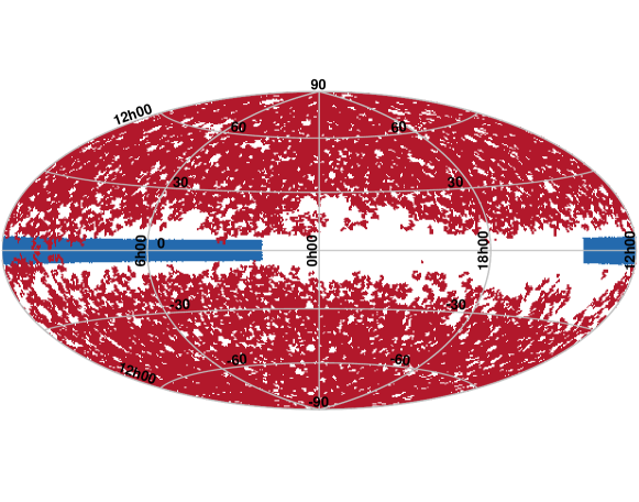
Figure 1: Red: Sky coverage of the GALEX catalogue GUVcat in Galactic coordinates. Blue: Sky coverage of IGAPS catalogue in Galactic coordinates. Only a small portion of the sky is in the footprint of both catalogues.

3 WD candidate selection

We selected WD candidates via colour-colour cuts that are defined by the intrinsic colours of hot-WD (e.g., Bianchi et al. 2011; Bianchi & Shiao 2020). In order to do so, we analysed a different set of UV-optical colour combinations. Figure 2 shows different colour-colour diagrams of the point-like (blue dots) and extended (black dots) sources, as defined in the tag Class from IGAPS, of the GaPHAS catalogue. We computed theoretical stellar colours for main-sequence (MS; red line) and supergiants (SG; brown line) stars using the stellar atmosphere models of Castelli & Kurucz (2003) for solar metallicity with $\log g=5.0$ and $\log g=3.0$, respectively, to guide the eye in the interpretation of the GaPHAS colours. We also calculated WD model colours (purple line) using the H-He non-LTE atmosphere models computed by Bianchi (2009); Bianchi et al. (2011), with the Tlusty code (Hubeny & Lanz 1995), with solar metallicity and $\log g=7.0$. A reddening vector with $E(B-V)=0.3$ mag is also shown in Figure 2 for a typical Milky-Way type dust, with $R_{V}=3.1$, using the Cardelli et al. (1989, hereafter CCM89) extinction law.

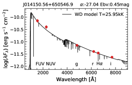
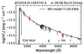
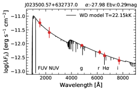
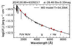
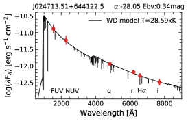
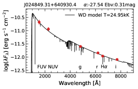
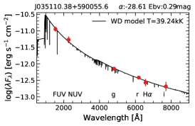
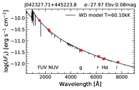
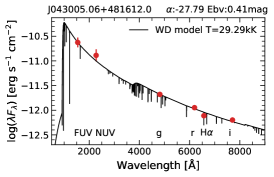
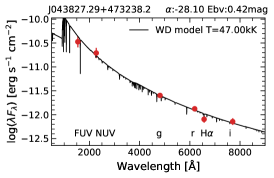
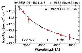
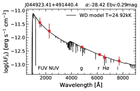
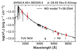
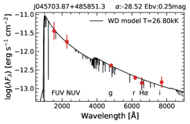
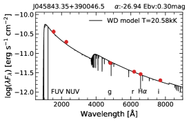
Figure 7: SED fit of the GALEX FUV and NUV + IGAPS g, r, i, and H$\alpha$ photometry (red dots) from which a single WD stars is infered. Synthetic spectrum of the best fit is also shown (black solid line).

In order to select reliable photometry of hot stellar sources from the GaPHAS catalogue, we selected the sources with the distancerank=0 and inversedistancerank=0 and with error cuts in optical and UV bands of 0.2 mag and 0.3 mag, respectively. We also removed the sources with the saturated=1 (from IGAPS catalogue) which indicates a saturated source in one or more than one optical bands. Similarly, we only selected FUV and NUV with magnitudes fainter than 13.73 and 13.85 mag, respectively (see Bianchi et al. 2018, for more information related to non-linearity limits). According to the work of Bianchi et al. (2011) the FUV$-$NUV$<-$0.13 colour cut corresponds to stellar $T_{\rm eff}$ hotter than 18 000 K (exact value might vary with gravity). Based on the Figure 7 of Bianchi et al. (2011), we set FUV$-$NUV$<-$0.53 colour cut in order to select stellar sources with $T_{\rm eff}$ hotter than 30 000 K (black dashed line in Figure 2) which covers the cases in which the hot-WD is young enough to still be likely to display a circumstellar ionised shell. The FUV$-$NUV colour selection also limits the contaminant sources such as galaxies and MS stars (e.g., Bianchi & Shiao 2020, and references therein; see Figure 2). A total of 74 sources were selected from the GaPHAS catalogue as probable hot-WD stellar sources (see Table 1; red dots in Figure 2) according to the FUV$-$NUV$<-$0.53 criteria. We also added a tag t50 indicating the sources with $T_{\rm eff}$ hotter than 50 000 K according to the FUV$-$NUV$<-$0.60 colour; a total of 52 sources are part of this group. Note that we only selected hot-WD candidates based on the FUV$-$NUV colour as it is usually less affected by the interstellar reddening (see $E(B-V)$ in Figure 2) and that other contaminants such as binary systems are not discarded (e.g., Bianchi et al. 2011; Raddi et al. 2017; Bianchi & Shiao 2020, for a review).

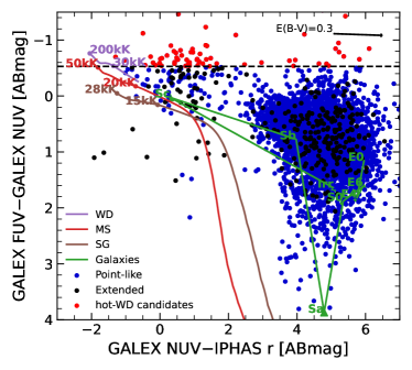
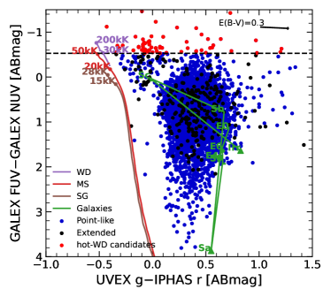
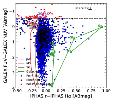
Figure 2: Color-color diagrams for IGAPS sources matched with GALEX UV sources. IGAPS point-like and extended sources are blue and black density points, respectively. The hot WD cooling sequence (purple line), the main-sequence (MS; red line), and the supergiant (SG; brown line) stellar sequences are for log(g) = 7.0, 5.0 and 3.0, respectively. Galaxy templates are shown in green for different morphologies labelled in the figure (E0, E4, E6, Sa, Sb, Sc, and Irr). Reddening vector for $E(B-V)=0.3$ mag is also shown in the upper-right side on each panel. The black dashed line indicates the cut of the hot WD candidates (red dots) using the FUV$-$NUV$-<$0.53 colour cut.

3.1 Matching WD candidates with Gaia EDR3

Distances from Gaia EDR3 (Gaia Collaboration 2020) were included for the WD star candidates shown in Table 1 when available. Because of the difference in epochs between IGAPS (which is in the Gaia DR2 reference frame) and Gaia EDR3 ( up to 12 yr) we need to account for stellar proper motions (see section 2.2 and section 4 of Raddi et al. 2017; Monguió et al. 2020, , respectively). First, we matched the list of WD candidates shown in Table 1 to Gaia EDR3 (Gaia Collaboration 2020) using a matching radius of 1′. The Gaia coordinates were converted to IGAPS observational epoch using the topcat Gaia command epochProp. Then, we re-calculated the sky distance between the Gaia propagated and IGAPS set of coordinates. Finally, the closest Gaia EDR3 match to the IGAPS coordinates was selected. The Gaia EDR3 Source column was used to match the WD stars with the Bayesian statistical distances from Bailer-Jones et al. (2021). Reported distances are only those with errors $\leq$30% resulting in 40 WD stars with reliable distances (see Table 1). Of these, only 30 were previously classified as WD candidates by Gentile Fusillo et al. (2021) (detGF in Table 1) by means of Gaia colour-colour diagrams and SDSS spectra.

In addition, we also tagged all WD stars that are reported with H$\alpha$ flux excess by matching the WD stars with the Fratta et al. (2021, Population-based identification of H $\alpha$-excess sources in the Gaia DR2 and IPHAS catalogues) by matching the Gaia EDR3 object ids. The Ha flux excess flag is also included in Table 1 when available; 17 WD star candidates are reported to have H$\alpha$ excess.

3.2 Matching WD candidates with 2MASS and UKIDDS

We matched the WD candidates with the Two-Micron All-Sky Survey Point Source Catalogue (2MASS PSC; Skrutskie et al. 2006) and with the UKIRT Infrared Deep Sky Survey (UKIDSS DR11; Lawrence et al. 2007; Almaini et al. 2007) using a matching radius of 1″, resulting in a 23 and 27 WD candidates with IR measurements, respectively. Note that we only account for matches with the information on the three J, H, and K bands, simultaneously.

Table 1: WD star candidates found between GALEX and IGAPS catalogues.

IGAPS Name	RAJ2000	DEJ2000	FUV	NUV	g	r	i	H$\alpha$	$r_{\rm geo}$	detGF	t50	H$\alpha^{\rm ex}$
			(mag)						(pc)
J012902.52+644429.1	01:29:02.52	+64:44:29.1	17.86	18.46	18.48	18.66	18.93	18.99	246.94	1	0	1
J014150.56+650546.9	01:41:50.56	+65:05:46.9	18.64	19.31	17.90	17.83	17.85	17.84	2175.63	0	1	0
J015418.01+654741.6	01:54:18.01	+65:47:41.6	19.81	20.59	19.59	19.63	19.93	20.10	320.34	1	1	1
J023215.29+632115.9	02:32:15.29	+63:21:15.9	19.96	20.50	16.08	15.58	15.34	15.59	5715.61	0	0	0
J023223.07+632040.9	02:32:23.07	+63:20:40.9	20.27	20.84	16.39	15.98	15.81	16.07	3837.86	0	0	1
J023500.57+632737.0	02:35:00.57	+63:27:37.0	20.09	20.84	19.60	19.67	19.99	19.87	371.75	1	1	0
J023527.80+632738.4	02:35:27.80	+63:27:38.4	20.67	21.52	16.91	16.39	16.14	16.43	7173.46	0	1	0
J024130.89+632923.7	02:41:30.89	+63:29:23.7	18.85	19.58	19.28	19.37	19.59	19.52	967.14	1	1	0
J024713.51+644122.5	02:47:13.51	+64:41:22.5	19.60	20.38	19.45	19.48	19.76	19.62	731.35	1	1	0
J024849.31+640930.4	02:48:49.31	+64:09:30.4	18.87	19.43	18.53	18.57	18.73	18.75	390.29	1	0	0
J024933.98+643643.0	02:49:33.98	+64:36:43.0	18.44	20.65	. . .	21.71	20.25	. . .	. . .	0	1	0
J025236.54+544506.9	02:52:36.54	+54:45:06.9	20.45	21.35	20.08	19.98	19.83	20.51	308.61	1	1	0
J025319.52+544414.1	02:53:19.52	+54:44:14.1	18.99	19.57	18.65	17.91	17.35	17.75	378.97	0	0	1
J025931.05+550806.3	02:59:31.05	+55:08:06.3	19.53	20.10	19.31	19.27	19.45	19.57	492.87	1	0	0
J031048.65+530022.7	03:10:48.65	+53:00:22.7	20.08	20.82	19.26	19.15	19.03	19.17	739.68	1	1	0
J031936.06+531425.1	03:19:36.06	+53:14:25.1	19.90	20.55	19.27	19.20	19.31	19.45	474.87	1	1	1
J032807.05+525737.0	03:28:07.05	+52:57:37.0	18.24	18.85	18.32	18.42	18.61	18.68	289.92	1	1	1
J033300.67+604529.5	03:33:00.67	+60:45:29.5	19.56	20.29	20.71	21.16	. . .	. . .	3592.07	0	1	0
J033300.81+524748.0	03:33:00.81	+52:47:48.0	18.38	19.10	18.44	18.47	18.59	18.61	340.38	1	1	1
J034015.23+615204.1	03:40:15.23	+61:52:04.1	19.04	20.47	15.79	15.06	14.81	14.96	894.44	0	1	0
J034631.63+590920.2	03:46:31.63	+59:09:20.2	18.98	19.75	19.20	19.28	19.38	19.42	628.46	1	1	1
J035010.66+600113.9	03:50:10.66	+60:01:13.9	19.46	20.00	19.98	19.95	20.23	20.19	500.34	1	0	0
J035110.38+590055.6	03:51:10.38	+59:00:55.6	19.31	19.99	19.80	19.93	20.16	20.19	636.55	1	1	0
J035737.37+570303.8	03:57:37.37	+57:03:03.8	19.64	21.78	15.83	15.11	14.75	14.99	8979.38	0	1	0
J035934.41+571348.5	03:59:34.41	+57:13:48.5	19.82	20.40	16.17	15.76	15.60	15.83	2872.91	0	0	1
J040144.53+461434.1	04:01:44.53	+46:14:34.1	20.44	21.05	19.84	19.91	20.07	20.24	424.76	1	1	0
J040522.62+555339.4	04:05:22.62	+55:53:39.4	20.68	21.63	16.88	16.42	16.21	16.44	6377.98	0	1	0
J040613.18+561233.9	04:06:13.18	+56:12:33.9	20.98	21.63	20.88	20.85	20.87	20.99	2913.53	0	1	0
J041039.52+444840.9	04:10:39.52	+44:48:40.9	20.26	21.10	20.10	20.14	. . .	20.52	1192.50	1	1	0
J041531.64+450209.2	04:15:31.64	+45:02:09.2	20.31	20.89	19.68	19.64	19.67	19.93	232.96	1	0	1
J042327.71+445223.8	04:23:27.71	+44:52:23.8	15.56	16.25	17.22	17.55	17.88	17.74	163.48	1	1	1
J042553.88+441907.5	04:25:53.88	+44:19:07.5	20.67	21.21	20.48	20.35	20.54	20.59	3436.54	0	0	0
J042641.65+444404.7	04:26:41.65	+44:44:04.7	18.01	18.55	15.63	14.65	14.25	14.45	336.63	0	0	0
J042646.87+444612.3	04:26:46.87	+44:46:12.3	19.59	20.30	20.29	20.57	. . .	20.85	527.77	1	1	0
J042703.35+414349.2	04:27:03.35	+41:43:49.2	18.73	19.27	18.45	18.52	18.59	18.70	441.61	1	0	1
J042756.39+413000.6	04:27:56.39	+41:30:00.6	20.02	20.59	20.09	20.17	. . .	20.45	1112.97	0	0	0
J042837.29+411452.6	04:28:37.29	+41:14:52.6	20.48	21.13	20.70	20.61	21.04	21.15	1265.56	0	1	0
J043005.06+481612.0	04:30:05.06	+48:16:12.0	19.52	20.19	19.09	19.10	19.19	19.37	462.32	1	1	1
J043137.79+415249.2	04:31:37.79	+41:52:49.2	20.11	21.22	17.23	17.00	16.89	17.08	5853.45	0	1	0
J043143.43+415247.0	04:31:43.43	+41:52:47.0	19.48	21.22	16.38	15.78	15.48	15.76	2896.42	0	1	0
J043145.95+445458.7	04:31:45.95	+44:54:58.7	19.51	20.36	14.89	14.25	13.98	14.19	824.39	0	1	1
J043326.01+413116.1	04:33:26.01	+41:31:16.1	20.86	21.50	17.88	17.55	17.49	17.64	4620.90	0	1	0
J043519.17+543932.7	04:35:19.17	+54:39:32.7	20.11	20.74	18.17	16.96	16.28	16.71	650.68	0	1	0
J043827.29+473238.2	04:38:27.29	+47:32:38.2	19.20	19.80	18.91	18.94	19.07	19.35	257.75	1	1	1
J044326.63+464520.2	04:43:26.63	+46:45:20.2	17.64	18.46	18.83	17.86	17.35	17.76	2776.41	0	1	0
J044447.07+394243.0	04:44:47.07	+39:42:43.0	20.90	21.55	20.88	20.78	. . .	. . .	. . .	0	1	0
J044554.05+492824.2	04:45:54.05	+49:28:24.2	20.27	21.05	16.14	15.82	15.65	15.88	2982.53	0	1	1
J044635.04+480118.6	04:46:35.04	+48:01:18.6	19.95	21.42	20.78	20.88	21.06	21.08	. . .	0	1	0
J044639.01+402003.3	04:46:39.01	+40:20:03.3	19.90	20.70	20.26	20.29	20.15	20.41	3275.08	0	1	0
J044822.93+483429.1	04:48:22.93	+48:34:29.1	18.31	18.90	16.40	15.94	15.74	15.97	4499.73	0	0	0
J044839.59+483606.0	04:48:39.59	+48:36:06.0	16.35	17.44	15.64	15.23	15.05	15.26	5244.07	0	1	0
J044923.41+491440.4	04:49:23.41	+49:14:40.4	20.59	21.25	20.33	20.48	20.62	20.65	3046.80	0	1	0
J044925.36+490701.4	04:49:25.36	+49:07:01.4	19.53	20.09	20.18	20.52	. . .	. . .	1695.95	0	0	0
J045614.60+385509.5	04:56:14.60	+38:55:09.5	20.58	21.42	20.38	20.47	20.59	20.80	1152.69	1	1	0
J045703.87+485851.3	04:57:03.87	+48:58:51.3	20.26	20.82	20.24	20.56	20.45	20.80	937.39	1	0	0
J045739.49+505757.4	04:57:39.49	+50:57:57.4	15.57	16.21	16.93	17.24	17.53	17.41	296.33	1	1	1
J045809.37+390538.7	04:58:09.37	+39:05:38.7	18.34	19.00	18.86	18.99	19.06	19.21	605.61	1	1	0
J045841.57+364234.2	04:58:41.57	+36:42:34.2	19.52	20.08	17.88	17.61	17.59	17.68	1850.52	0	0	0
J045843.35+390046.5	04:58:43.35	+39:00:46.5	18.16	18.72	17.61	17.61	17.71	17.65	2003.94	0	0	0
J045854.82+482831.0	04:58:54.82	+48:28:31.0	18.94	19.49	19.55	19.62	19.85	19.80	1421.53	1	0	0
J045930.01+485819.9	04:59:30.01	+48:58:19.9	18.24	20.14	. . .	21.69	20.99	. . .	. . .	0	1	0
J045946.22+505231.8	04:59:46.22	+50:52:31.8	20.06	20.65	20.62	20.66	. . .	. . .	4101.53	0	0	0
J050117.70+485213.5	05:01:17.70	+48:52:13.5	16.02	16.58	21.45	20.25	19.57	20.15	2948.58	0	0	0
J050209.17+492513.9	05:02:09.17	+49:25:13.9	20.39	21.30	19.95	19.96	20.12	19.89	2083.38	1	1	0
J050405.54+383324.9	05:04:05.54	+38:33:24.9	20.19	20.89	16.10	15.53	15.25	15.58	5473.55	0	1	0
J050933.75+345104.9	05:09:33.75	+34:51:04.9	20.00	20.65	15.39	14.83	14.57	14.82	1308.39	0	1	0
J051008.24+321804.2	05:10:08.24	+32:18:04.2	19.75	20.44	19.86	19.95	20.27	20.40	740.52	1	1	0
J051112.03+344722.5	05:11:12.03	+34:47:22.5	19.43	20.08	19.54	19.00	18.30	18.78	736.67	0	1	0
J052925.68+402700.9	05:29:25.68	+40:27:00.9	19.88	20.41	19.03	18.96	19.00	19.09	5651.06	0	0	0
J053207.61+404445.3	05:32:07.61	+40:44:45.3	19.85	21.46	20.18	20.27	20.26	20.58	3120.23	0	1	0
J053659.57+395430.0	05:36:59.57	+39:54:30.0	19.61	20.73	20.80	21.23	. . .	21.17	. . .	0	1	0
J053955.63+395004.6	05:39:55.63	+39:50:04.6	20.05	20.95	20.47	20.63	20.73	21.03	847.64	0	1	0
J190347.51+170140.6	19:03:47.51	+17:01:40.6	19.45	20.97	. . .	16.23	16.14	16.29	3926.18	0	1	0
J190443.07+172843.4	19:04:43.07	+17:28:43.4	20.26	21.50	20.19	20.16	20.34	20.33	3770.48	0	1	0

Table 2: Single WDs stellar parameters derived using the MCMC method. The objects in bold are the hot WDs with $T_{\rm eff}\geq 50\,000$ K.

IGAPS Name	$T_{\rm WD}$	$\alpha$	d	$R_{\rm WD}$	$\log(L_{\rm WD})$	$E(B-V)$
	(103)		(kpc)	(R$\sun$)	($L\sun$)	(mag)
J014150.56+650546.9	26$\pm$1	-27.039$\pm$0.018	2.18$\pm^{0.54}_{0.37}$	0.174$\pm^{0.044}_{0.030}$	1.094$\pm^{0.220}_{0.151}$	0.450$\pm$0.010
J015418.01+654741.6	26$\pm$1	-28.085$\pm$0.054	0.32$\pm^{0.03}_{0.03}$	0.009$\pm^{0.001}_{0.001}$	-1.473$\pm^{0.134}_{0.132}$	0.310$\pm$0.035
J023500.57+632737.0	22$\pm$1	-27.977$\pm$0.056	0.37$\pm^{0.05}_{0.04}$	0.012$\pm^{0.002}_{0.001}$	-1.530$\pm^{0.165}_{0.137}$	0.290$\pm$0.040
J024130.89+632923.7	54$\pm$6	-28.478$\pm$0.050	0.97$\pm^{0.28}_{0.18}$	0.018$\pm^{0.005}_{0.004}$	0.420$\pm^{0.322}_{0.263}$	0.330$\pm$0.007
J024713.51+644122.5	29$\pm$2	-28.051$\pm$0.051	0.73$\pm^{0.18}_{0.11}$	0.021$\pm^{0.005}_{0.004}$	-0.563$\pm^{0.243}_{0.171}$	0.341$\pm$0.040
J024849.31+640930.4	25$\pm$1	-27.536$\pm$0.023	0.39$\pm^{0.02}_{0.02}$	0.019$\pm^{0.001}_{0.001}$	-0.898$\pm^{0.064}_{0.067}$	0.314$\pm$0.014
J035110.38+590055.6	39$\pm$5	-28.611$\pm$0.085	0.64$\pm^{0.17}_{0.12}$	0.011$\pm^{0.003}_{0.002}$	-0.620$\pm^{0.338}_{0.299}$	0.286$\pm$0.016
J042327.71+445223.8	60$\pm$2	-27.969$\pm$0.018	0.16$\pm^{0.00}_{0.00}$	0.005$\pm^{0.001}_{0.001}$	-0.503$\pm^{0.071}_{0.072}$	0.083$\pm$0.004
J043005.06+481612.0	29$\pm$1	-27.788$\pm$0.038	0.46$\pm^{0.07}_{0.05}$	0.018$\pm^{0.003}_{0.002}$	-0.691$\pm^{0.148}_{0.126}$	0.412$\pm$0.023
J043827.29+473238.2	47$\pm$6	-28.105$\pm$0.082	0.26$\pm^{0.01}_{0.01}$	0.007$\pm^{0.001}_{0.001}$	-0.652$\pm^{0.247}_{0.246}$	0.419$\pm$0.005
J044635.04+480118.6	106$\pm$42	-29.517$\pm$0.181	. . .	. . .	. . .	0.338$\pm$0.020
J044923.41+491440.4	25$\pm$2	-28.417$\pm$0.062	3.05$\pm^{2.29}_{1.67}$	. . .	. . .	0.290$\pm$0.052
J045614.60+385509.5	38$\pm$16	-28.653$\pm$0.167	1.15$\pm^{0.76}_{0.49}$	. . .	. . .	0.420$\pm$0.060
J045703.87+485851.3	27$\pm$2	-28.524$\pm$0.078	0.94$\pm^{1.43}_{0.39}$	. . .	. . .	0.250$\pm$0.050
J045843.35+390046.5	26$\pm$1	-27.008$\pm$0.015	2.00$\pm^{0.65}_{0.37}$	. . .	. . .	0.376$\pm$0.010
J050209.17+492513.9	27$\pm$2	-28.116$\pm$0.056	2.08$\pm^{0.77}_{0.97}$	. . .	. . .	0.400$\pm$0.040
J051008.24+321804.2	49$\pm$14	-28.682$\pm$0.130	0.74$\pm^{0.46}_{0.21}$	. . .	. . .	0.345$\pm$0.041
J053955.63+395004.6	49$\pm$42	-28.977$\pm$0.262	0.85$\pm^{0.61}_{0.38}$	. . .	. . .	0.340$\pm$0.032
J190443.07+172843.4	97$\pm$47	-28.904$\pm$0.227	3.77$\pm^{2.05}_{1.45}$	. . .	. . .	0.510$\pm$0.023

Table 3: Binary WD stellar parameters determined with the MCMC method. The objects in bold are the hot WDs with $T_{\rm eff}\geq 50\,000$ K

IGAPS Name	$T_{\rm WD}$	$T_{\rm S}$	$\alpha$	$\beta$	d	$R_{\rm WD}$	$R_{\rm S}$	$\log(L_{\rm WD})$	$E(B-V)$
	(103)				(kpc)	(R$\sun$)		(L$\sun$)	(mag)
J012902.52+644429.1	100$\pm$3	9$\pm$1	-29.719$\pm$0.006	11.767$\pm$2.265	0.25$\pm^{0.01}_{0.01}$	0.001$\pm^{0.001}_{0.001}$	0.016$\pm^{0.003}_{0.003}$	-0.775$\pm^{0.057}_{0.052}$	0.008$\pm$0.004
J023215.29+632115.9	140$\pm$20	7$\pm$1	-29.507$\pm$0.012	104.473$\pm$21.832	5.72$\pm^{1.05}_{0.80}$	0.039$\pm^{0.007}_{0.005}$	4.059$\pm^{1.129}_{1.023}$	2.720$\pm^{0.293}_{0.275}$	0.380$\pm$0.085
J023223.07+632040.9	190$\pm$18	8$\pm$1	-29.553$\pm$0.003	80.582$\pm$14.037	3.84$\pm^{0.64}_{0.46}$	0.025$\pm^{0.004}_{0.003}$	2.006$\pm^{0.484}_{0.423}$	2.862$\pm^{0.218}_{0.192}$	0.460$\pm$0.033
J023527.80+632738.4	28$\pm$2	8$\pm$1	-28.000$\pm$0.003	16.119$\pm$16.160	. . .	. . .	. . .	. . .	0.495$\pm$0.015
J025236.54+544506.9	98$\pm$15	8$\pm$1	-29.677$\pm$0.036	9.756$\pm$2.770	0.31$\pm^{0.04}_{0.03}$	0.002$\pm^{0.001}_{0.001}$	0.017$\pm^{0.005}_{0.005}$	-0.580$\pm^{0.289}_{0.275}$	0.328$\pm$0.025
J025319.52+544414.1	27$\pm$1	4$\pm$1	-28.175$\pm$0.004	24.160$\pm$0.623	0.38$\pm^{0.01}_{0.01}$	0.010$\pm^{0.001}_{0.001}$	0.236$\pm^{0.011}_{0.011}$	-1.321$\pm^{0.037}_{0.039}$	0.206$\pm$0.007
J025931.05+550806.3	47$\pm$4	9$\pm$1	-28.661$\pm$0.027	3.635$\pm$0.546	0.49$\pm^{0.07}_{0.06}$	0.008$\pm^{0.001}_{0.001}$	0.028$\pm^{0.006}_{0.006}$	-0.573$\pm^{0.207}_{0.193}$	0.330$\pm$0.006
J031048.65+530022.7	27$\pm$1	4$\pm$1	-27.772$\pm$0.030	5.141$\pm$1.104	. . .	. . .	. . .	. . .	0.444$\pm$0.050
J031936.06+531425.1	101$\pm$9	9$\pm$1	-29.814$\pm$0.013	14.388$\pm$5.058	0.47$\pm^{0.06}_{0.07}$	0.002$\pm^{0.001}_{0.001}$	0.034$\pm^{0.013}_{0.013}$	-0.282$\pm^{0.183}_{0.197}$	0.226$\pm$0.027
J032807.05+525737.0	71$\pm$2	9$\pm$1	-29.229$\pm$0.005	9.240$\pm$1.466	0.29$\pm^{0.01}_{0.01}$	0.003$\pm^{0.001}_{0.001}$	0.024$\pm^{0.004}_{0.004}$	-0.814$\pm^{0.062}_{0.062}$	0.109$\pm$0.014
J033300.81+524748.0	77$\pm$3	8$\pm$1	-29.209$\pm$0.007	10.272$\pm$3.801	0.34$\pm^{0.02}_{0.02}$	0.003$\pm^{0.001}_{0.001}$	0.032$\pm^{0.012}_{0.012}$	-0.508$\pm^{0.077}_{0.075}$	0.147$\pm$0.042
J034015.23+615204.1	154$\pm$18	6$\pm$1	-28.872$\pm$0.012	92.356$\pm$13.522	0.89$\pm^{0.02}_{0.02}$	0.011$\pm^{0.001}_{0.001}$	1.059$\pm^{0.157}_{0.157}$	1.825$\pm^{0.209}_{0.209}$	0.459$\pm$0.007
J034631.63+590920.2	87$\pm$3	9$\pm$1	-29.485$\pm$0.009	8.864$\pm$3.435	0.63$\pm^{0.09}_{0.07}$	0.004$\pm^{0.001}_{0.001}$	0.039$\pm^{0.016}_{0.016}$	-0.015$\pm^{0.138}_{0.116}$	0.169$\pm$0.049
J035010.66+600113.9	32$\pm$2	8$\pm$2	-28.570$\pm$0.055	1.535$\pm$3.744	0.50$\pm^{0.13}_{0.08}$	0.009$\pm^{0.002}_{0.002}$	0.013$\pm^{0.033}_{0.033}$	-1.139$\pm^{0.250}_{0.173}$	0.230$\pm$0.008
J035737.37+570303.8	200$\pm$12	6$\pm$1	-29.895$\pm$0.002	265.645$\pm$22.274	. . .	. . .	. . .	. . .	0.310$\pm$0.030
J035934.41+571348.5	147$\pm$17	7$\pm$1	-29.465$\pm$0.012	83.334$\pm$14.470	2.87$\pm^{0.31}_{0.25}$	0.020$\pm^{0.002}_{0.002}$	1.697$\pm^{0.349}_{0.331}$	2.242$\pm^{0.222}_{0.215}$	0.386$\pm$0.010
J040144.53+461434.1	130$\pm$25	10$\pm$1	-30.578$\pm$0.014	19.045$\pm$4.821	0.42$\pm^{0.11}_{0.08}$	0.001$\pm^{0.001}_{0.001}$	0.019$\pm^{0.007}_{0.006}$	-0.596$\pm^{0.400}_{0.368}$	0.152$\pm$0.041
J040522.62+555339.4	151$\pm$24	7$\pm$1	-30.206$\pm$0.003	140.513$\pm$23.329	6.38$\pm^{1.46}_{1.32}$	0.022$\pm^{0.005}_{0.004}$	3.028$\pm^{0.857}_{0.805}$	2.338$\pm^{0.337}_{0.327}$	0.313$\pm$0.031
J040613.18+561233.9	43$\pm$7	8$\pm$1	-29.840$\pm$0.039	7.162$\pm$5.358	. . .	. . .	. . .	. . .	0.190$\pm$0.100
J041531.64+450209.2	122$\pm$20	9$\pm$1	-30.096$\pm$0.017	15.296$\pm$4.383	0.23$\pm^{0.03}_{0.02}$	0.001$\pm^{0.001}_{0.001}$	0.013$\pm^{0.004}_{0.004}$	-0.818$\pm^{0.314}_{0.303}$	0.236$\pm$0.035
J042553.88+441907.5	48$\pm$8	8$\pm$1	-30.120$\pm$0.026	11.777$\pm$6.844	. . .	. . .	. . .	. . .	0.100$\pm$0.060
J042641.65+444404.7	41$\pm$1	4$\pm$1	-29.060$\pm$0.012	182.122$\pm$51.271	0.34$\pm^{0.01}_{0.01}$	0.004$\pm^{0.001}_{0.001}$	0.651$\pm^{0.184}_{0.184}$	-1.498$\pm^{0.054}_{0.053}$	0.021$\pm$0.021
J042703.35+414349.2	50$\pm$3	9$\pm$1	-29.161$\pm$0.006	9.109$\pm$2.279	0.44$\pm^{0.04}_{0.04}$	0.004$\pm^{0.001}_{0.001}$	0.039$\pm^{0.010}_{0.010}$	-1.001$\pm^{0.118}_{0.113}$	0.122$\pm$0.020
J042837.29+411452.6	94$\pm$14	8$\pm$1	-30.514$\pm$0.030	12.903$\pm$4.285	. . .	. . .	. . .	. . .	0.100$\pm$0.070
J043137.79+415249.2	198$\pm$15	8$\pm$1	-30.239$\pm$0.002	82.734$\pm$11.700	. . .	. . .	. . .	. . .	0.260$\pm$0.020
J043143.43+415247.0	172$\pm$13	6$\pm$1	-29.574$\pm$0.011	124.632$\pm$11.675	2.90$\pm^{0.36}_{0.34}$	0.018$\pm^{0.002}_{0.002}$	2.293$\pm^{0.358}_{0.345}$	2.427$\pm^{0.172}_{0.168}$	0.343$\pm$0.010
J043145.95+445458.7	152$\pm$19	6$\pm$1	-29.870$\pm$0.011	345.047$\pm$51.821	0.82$\pm^{0.02}_{0.02}$	0.004$\pm^{0.001}_{0.001}$	1.344$\pm^{0.204}_{0.205}$	0.863$\pm^{0.218}_{0.218}$	0.248$\pm$0.086
J043326.01+413116.1	195$\pm$20	7$\pm$1	-30.768$\pm$0.003	114.280$\pm$18.479	. . .	. . .	. . .	. . .	0.210$\pm$0.040
J043519.17+543932.7	121$\pm$11	4$\pm$1	-30.431$\pm$0.003	377.559$\pm$99.229	0.65$\pm^{0.05}_{0.05}$	0.002$\pm^{0.001}_{0.001}$	0.662$\pm^{0.182}_{0.182}$	-0.221$\pm^{0.171}_{0.172}$	0.123$\pm$0.040
J044554.05+492824.2	143$\pm$23	8$\pm$1	-29.372$\pm$0.004	73.031$\pm$13.000	2.98$\pm^{0.31}_{0.23}$	0.023$\pm^{0.002}_{0.002}$	1.694$\pm^{0.349}_{0.329}$	2.309$\pm^{0.296}_{0.290}$	0.474$\pm$0.029
J044639.01+402003.3	30$\pm$2	4$\pm$2	-28.675$\pm$0.055	10.425$\pm$3.378	. . .	. . .	. . .	. . .	0.240$\pm$0.114
J044822.93+483429.1	22$\pm$1	6$\pm$1	-26.894$\pm$0.013	6.679$\pm$0.849	4.50$\pm^{1.34}_{0.82}$	0.417$\pm^{0.125}_{0.077}$	2.786$\pm^{0.905}_{0.622}$	1.564$\pm^{0.262}_{0.163}$	0.350$\pm$0.019
J044839.59+483606.0	49$\pm$2	5$\pm$1	-26.555$\pm$0.020	8.391$\pm$0.874	5.24$\pm^{1.11}_{0.76}$	0.682$\pm^{0.145}_{0.100}$	5.722$\pm^{1.353}_{1.030}$	3.368$\pm^{0.200}_{0.149}$	0.523$\pm$0.009
J045739.49+505757.4	62$\pm$1	9$\pm$1	-28.205$\pm$0.006	4.171$\pm$0.282	0.30$\pm^{0.01}_{0.01}$	0.007$\pm^{0.001}_{0.001}$	0.031$\pm^{0.002}_{0.002}$	-0.126$\pm^{0.034}_{0.036}$	0.029$\pm$0.012
J045809.37+390538.7	49$\pm$3	8$\pm$1	-28.613$\pm$0.018	3.499$\pm$0.338	0.61$\pm^{0.11}_{0.08}$	0.010$\pm^{0.002}_{0.001}$	0.035$\pm^{0.007}_{0.006}$	-0.280$\pm^{0.186}_{0.154}$	0.213$\pm$0.005
J045841.57+364234.2	102$\pm$5	7$\pm$1	-30.248$\pm$0.002	61.904$\pm$17.079	. . .	. . .	. . .	. . .	0.070$\pm$0.024
J045854.82+482831.0	59$\pm$4	8$\pm$1	-29.829$\pm$0.010	10.439$\pm$4.919	. . .	. . .	. . .	. . .	0.001$\pm$0.025
J050405.54+383324.9	118$\pm$21	8$\pm$1	-28.479$\pm$0.012	40.139$\pm$13.803	5.47$\pm^{1.02}_{0.88}$	0.104$\pm^{0.019}_{0.017}$	4.175$\pm^{1.634}_{1.587}$	3.271$\pm^{0.353}_{0.343}$	0.650$\pm$0.006
J050933.75+345104.9	144$\pm$24	7$\pm$1	-29.643$\pm$0.011	190.016$\pm$37.862	1.31$\pm^{0.06}_{0.05}$	0.008$\pm^{0.001}_{0.001}$	1.475$\pm^{0.302}_{0.299}$	1.366$\pm^{0.289}_{0.288}$	0.360$\pm$0.010
J052925.68+402700.9	66$\pm$7	8$\pm$1	-29.997$\pm$0.006	20.727$\pm$10.184	. . .	. . .	. . .	. . .	0.090$\pm$0.050
J053207.61+404445.3	161$\pm$36	9$\pm$1	-30.367$\pm$0.015	20.873$\pm$16.554	. . .	. . .	. . .	. . .	0.202$\pm$0.100

Table 4: WD stars classification according to the regions defined by Wellhouse et al. (2005). The objects in bold are the hot WDs with $T_{\rm eff}\geq 50\,000$ K.

IGAPS Name	Region2MASS	RegionUKIDSS
J023215.29+632115.9	III
J023223.07+632040.9	III
J023527.80+632738.4	I
J025319.52+544414.1	II
J031048.65+530022.7		III
J033300.81+524748.0		IV
J034015.23+615204.1	I
J035737.37+570303.8	I	I
J035934.41+571348.5	I	I
J040522.62+555339.4	I	I
J041531.64+450209.2		I
J042641.65+444404.7	II	II
J042703.35+414349.2		IV
J043137.79+415249.2	I	I
J043143.43+415247.0	I	I
J043145.95+445458.7	I	I
J043326.01+413116.1	II	III
J043519.17+543932.7	II
J044326.63+464520.2	III	III
J044554.05+492824.2	I	I
J044822.93+483429.1	I	I
J044839.59+483606.0	I	I
J045739.49+505757.4		I
J045809.37+390538.7		III
J045841.57+364234.2	II	I
J045843.35+390046.5		I
J045930.01+485819.9		II
J050117.70+485213.5		II
J050405.54+383324.9	I	III
J050933.75+345104.9	I	I
J051112.03+344722.5	II	II
J052925.68+402700.9		IV
J190347.51+170140.6	III	I

4 SED fitting

We estimated the physical parameters ($T_{\rm eff}$, radius, and interstellar reddening) of the candidates by performing fits of their spectral energy distributions (SED).

Theoretically, the equation that describes the magnitude observed of any source in the AB magnitude system, is

$$m_{\rm AB}=-2.5\log\left(F_{\nu}\left[e^{\alpha}\right]^{2}\right)-48.6$$ (1)

with

$$\alpha\equiv\ln\left(\frac{R_{1}}{D}\right)$$

where $R$ is the radius of the star, D is the distance to it, and $F_{\nu}=F_{\nu}\left(T_{\rm eff},\log(g),Z\right)$ the flux of the star at frequency $\nu$. The total number of free parameters are five: $R$, $D$, $T_{\rm eff}$, $\log(g)$, and the metallicity, $Z$.

Equation 1 would be enough to fit any WD star. However, it is difficult to achieve accurate values of stellar parameters ($T_{\rm WD}$, $R_{\rm WD}$) with few observable variables (2 points from GALEX, when available, and 4 points from IGAPS). To reduce the number of free parameters, we fitted colour indexes instead of magnitudes as follows,

$$m_{\rm A}-m_{\rm B}=-2.5\log\left(F_{\rm A}/F_{\rm B}\right)$$ (2)

which remove the stellar radius,$R$, and the distance to the object. The A and B subscripts indicate the magnitude difference between filter A and B.

In the case of binary systems, equation 2 transforms to

$$m_{\rm A}-m_{\rm B}=-2.5\log\left(\frac{F^{1}_{\rm A}+F^{2}_{\rm A}\beta^{2}}{F^{1}_{\rm B}+F^{2}_{\rm B}\beta^{2}}\right)$$ (3)

where

$$\beta\equiv R_{2}/R_{1}.$$

Note that in all the equations the flux is accounting for the extinction in the following form,

$$F_{\nu}=f_{\nu}10^{0.4E(B-V)X_{\lambda}}$$ (4)

where $f_{\nu}$ is the observed flux, and $X_{\lambda}$ is the extinction coefficient according to Cardelli et al. (1989) extinction law.

A Nelder-Mead algorithm (NMA) was employed to find the best fit to the equation 2 (and equation 3 in the case of binary systems) and then equation 1. Appropriate atmosphere models for WD stars and for MS stars, for possible cool companions, were selected. The H-He non-LTE TLUSTY (Hubeny & Lanz 1995) solar atmosphere models for the hot-WD stars (Bianchi 2009; Bianchi et al. 2011) were used, which covers a range of effective temperature, $T_{\rm eff}$, from 20 000 K$<T_{\rm eff}<$200 000 K and a range of gravities of 4.0$<\log g<$9.0. For the MS stars the solar LTE BT-Settl stellar atmosphere models from Phoenix/NextGen group (Hauschildt et al. 1999; Allard et al. 2012) which covers a range from 2600 K$<T_{\rm eff}<$15 000 K and $-0.5<\log g<5.5$ were used. Each atmosphere model was convolved with the GALEX and IGAPS transmission curves in order to create a grid of synthetic flux models. It is important to mention that we fixed the value of $\log g$= 5 and 7 for MS and WD atmosphere models, respectively, as have been proven that $\log g$ is not very sensitive to colour indexes (see Barker et al. 2018). After NMA fitting, we sampled the posterior probability of the stellar parameters using the Markov-Chain Monte-Carlo (MCMC) through the emcee (Foreman-Mackey et al. 2013) python package.

The fitting procedure of each object was as follows. First, we run the NMA fitting procedure, taking the equation 2 as a kernel (or equation 3 if a binary is guessed), to first estimate the stellar parameters and $E(B-V)$, and calculate their posterior probability with the MCMC algorithm. For this, we reddened the theoretical spectra and convolved with GALEX and IGAPS bands on the fly, varying the $E(B-V)$ according to equation 4. For objects with reliable Gaia distances, we set the $E(B-V)$ and the error (as obtained using Bayestar2019; Green et al. 2019) as priors to the MCMC run. For Bayestar2019, we only selected $E(B-V)$ values and distances that contained both ’reliable_dist’ and ’converged’ flags set to True. For cases where the value of $E(B-V)$ could not be obtained using Bayestar2019, we selected the reddening value from GUVcat catalogue (which is calculated using the extinction map of Schlegel et al. 1998) and varied $E(B-V)$ from 0 to GUVcat $E(B-V)$ value.

A second run was used to obtain the marginalised posterior distribution of the stellar parameters of the star (or binary system) by first using equation 2, to obtain $T_{\rm WD}$ (and $\beta$ and $T_{\rm MS}$ if a binary system is previously fitted), and then equation 1 to obtain the scaling factor, $\alpha$. Note that for the second run we fixed the value of $E(B-V)$ as resulted from the first run; the observed magnitudes were previously unreddened with this value to be compared with the grid of theoretical flux models.

Table 2 shows the stellar parameters resulted from the MCMC method of single WD stars along with the $E(B-V)$ value. Most of the WD stars have an $T_{\rm eff}<50\,000$ K with only four greater than 50 000 K. Table 3 shows the objects for which a binary system was fitted. In this case, a total of 27 binary systems contain WD stars with $T_{\rm WD}>50\,000$ K. Note that sources with more than one missing magnitude measurement were not fitted because of MCMC convergence problems (i.e., MCMC did not converge due to a few observable values). Stellar radius was calculated using Gaia distances and $\alpha$ whereas the luminosity was calculated using the Stefan-Boltzmann luminosity relation.

Gaia EDR3 provides a direct measurement of distance for the majority of the WD stars candidates of our sample. Most of them with distances $<$1 kpc and only ten with distances $>$1 kpc. The combination of Gaia EDR3 distances allowed us to concurrently determine the stellar radius of the WD and binary WD candidates, using the distance to solve the $\alpha$ and $\beta$ parameters, and its luminosity, $L_{\rm WD}$. Figure 3 shows the H-R diagram of the WD (blue) and binary WD candidates (red) along with the low- and intermediate-mass stars theoretically evolutionary tracks of Miller Bertolami (2016, MB2016) and the low-mass He- and O-core WD tracks of Panei et al. (2007, Pa2007). Note that for MB2016 models we linearly extended the theoretical tracks to account for luminosities below of $\log(L/L_{\odot})<0.$ instead of the limit of $\log(L/L_{\odot})=1$ as the original ones. The evolutionary stage of the majority of the objects corresponds to the WD cooling track except for four objects whose evolutionary stage corresponds to the constant luminosity phase for low mass stars (J044839.59+483606.0, J050405.54+383324.9, J044822.93+483429.1, and J014150.56+650546.9).

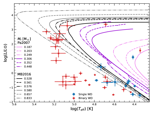
Figure 3: H-R diagram showing the single (blue) and binary (red) WD candidates in conjunction with the low- and intermediate-mass stars theoretical tracks of MB2016 (gray lines) and the He- and O-core WD tracks of Pa2007 (purple lines). Masses of the evolutionary tracks are labelled in the figure.

In Figure 4, we show the IGAPS colour-magnitude (CMD) diagram of the candidate WDs. For reference, we plot the MESA/MIST (Choi et al. 2016, and references therein) evolutionary tracks for stars of 1–4 M_⊙ and the La Plata cooling tracks for WDs of 0.2–1.2 M_⊙ with hydrogen-rich atmospheres (Althaus et al. 2013; Camisassa et al. 2016; Camisassa et al. 2019). The absolute magnitudes of WDs were computed by means of appropriate synthetic spectra (Koester 2010).

We converted the IGAPS magnitudes of the candidate WDs into absolute magnitudes by using the $E(V-B)$ and distances from Tables 2 and 3. The single WD stars from the GaPHAS catalogue appear in the WD cooling phase, as expected, in the CMD whereas the colours of the binary WD stars are scattered around in the CMD due to the blending of the two components; a few of them overlap with the main-sequence (MS) while others are close to the WD cooling sequence. Binary objects that are located in the MS loci are dominated by the flux of the companion star in the optical range (e.g., J023215.29+632115.9, J0333.07+632040.9, and J040522.62+555339.4) whereas the magnitude of the binary objects located close to the WD loci is the composition of both the WD and the binary companion flux (e.g., J045739.49+505757.4, J025931.05+550806.3, and J045809.37+390538.7). One additional problem is that for these hot and very hot stars, a small $T_{\rm eff}$ uncertainty may actually mean a large uncertainty in the reddening/extinction and hence affecting the position in the CMD; the latter could be solved by spectroscopic observations.

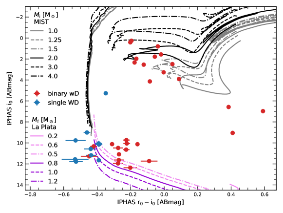
Figure 4: Colour-magnitude diagram using the MIST theoretical tracks (gray/black lines) and La Plata WD cooling tracks (purple lines) for different initial masses (labelled in the figure). Single (blue dots) and binary (red dots) WD candidates are also shown.

5 Discussion

In the following subsections, we present the discussion of the SED fitting in terms of the estimated stellar parameters and their comparison with different theoretical evolutionary tracks. We also discuss the WD candidates classification on infrared (IR) colour-colour maps as well as the nature of the binary companions found in our sample. Finally, a discussion related to the nebulae around WD star candidates is also included.

5.1 Physical properties of WD candidates

The combination of GALEX FUV and NUV, and IGAPS g r H$\alpha$ i, analysed with synthetic spectra, enable a preliminary characterisation of the WD and unresolved binary WD candidates (see e.g., Bianchi et al. 2018). Figures 7 to 11 show the best fitted synthetic spectrum to the UV-optical photometry, as extracted from GaPHAS catalogue, for single and binary WD candidates, respectively. The majority of the fitted $T_{\rm eff}$ correspond to the $T_{\rm eff}$ expected from the GALEX FUV$-$NUV colour; the GALEX FUV$-$NUV$<-$0.53 corresponds to $T_{\rm eff}\geq$30 000 K (see Figure 7 of Bianchi et al. 2011). However, large errors in the photometry could strongly affect the position of the WD stars in the colour-colour diagrams presented in Figure 2. Objects with GALEX colours FUV$-$NUV$\sim-$0.53 but large errors could result in smaller or higher $T_{\rm eff}$ during the fitting procedure; this could be the case for objects resulting with $T_{\rm eff}<$30 000 K. This can also occur when the binary companion contributes to the overall flux in the GALEX NUV band (e.g., J023527.80+632738.4 and J044822.93+483429.1).

As mentioned in section 4 the stellar parameters were obtained by fitting the different combinations of colour indexes between GALEX and IGAPS catalogues by the implementation of the MCMC algorithm. Most of the fitted parameters are very well constrained between 20 000 K$\leq T_{\rm eff}\leq$100 000 K, however, for $T_{\rm eff}>$100 000 K the fitting is not accurate because colour indexes, specially GALEX FUV$-$NUV (see Figure 7 Bianchi et al. 2011), are not very sensitive to higher effective temperatures. Objects resulting with $T_{\rm eff}>$100 000 K must be taken as an upper limit and must be combined with spectral data in order to corroborate its nature.

Figure 5 show the total number of single and binary WD candidates obtained from the SED fitting. Out of the 74 WD candidates, a total of 41 resulted in probably binary systems in which a binary fraction of 55.4% is estimated, similar to the binary fractions expected for solar-like and M-type MS stars (e.g., Raghavan et al. 2010; Winters et al. 2019) and lower than the fraction of binary central stars of PNe ($\sim$70%; De Marco et al. 2013; Jones & Boffin 2017).

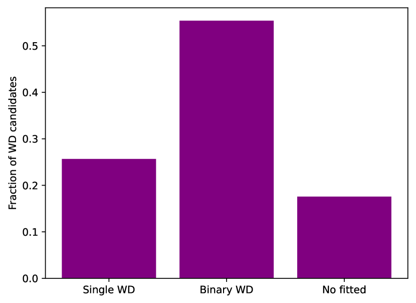
Figure 5: Fraction of single and binary WD star candidates from the GaPHAS catalogue resulted from the fitting procedure. The fraction of WD stars that were not fitted is also shown. A binary fraction of 55% was estimated.

5.2 WD classification

According to Wellhouse et al. (2005), the infrared colour-colour diagrams of WDs can be classified into four different regions that are occupied by: I) single WDs; II) binary WDs with colours dominated by a low-mass late MS companions or a very low-mass L-type companions; III) binary WDs that have very low-mass brown dwarf companions; IV) objects with colours that are probably contaminated by the presence of circumstellar material (see Figure 1 from Wellhouse et al. 2005). In this context, an analysis of the IR 2MASS and UKIDSS colour indexes of the WD stars that are shown in Table 1 was performed. Figure 6 shows the colour-colour diagrams for 2MASS (top) and UKIDSS (bottom) colour indexes. In the 2MASS diagram we identified 13 objects in region I, 6 in region II, 4 in region III, and none in region IV. In the UKIDSS diagram we found 15 objects in region I, 4 in region II, 5 in region III, and 3 in region IV. Only 13 WD candidates (ten of which are part of the region I) coincide in terms of identification in both diagrams.
We notice that objects selected as single in Fig.6 are also described as such based on their SED analysis (2). The same applies to those classified as binary WDs (3). This is underlying the strength of the method used in Section 4.

The objects present in region III are of particular interest as they might be a case of a WD with a planetary companion, although a low mass brown dwarf is not discarded. We, therefore, performed a search in the Transiting Exoplanet Survey Satellite (TESS) database (Ricker et al. 2015) for all the objects in regions III and IV. We expect this investigation to be completed by follow-up observations using ground-based facilities in order to obtain more accurate information on the binary parameters.

5.3 Nature of the binary companion

Due to these targets mostly being faint and located in crowded fields, they received low priority in the TESS Candidate Target List (CTL; Stassun et al. 2018) and were therefore not selected for short-cadence observations. We created light curves from the TESS full-frame images (FFIs) using the eleanor Python package (Feinstein et al. 2019), by specifying the target coordinates. We then detrended these raw light curves by two different methods; 1) by regressing against background level and co-trending basis vectors from eleanor; and 2) by a 10-hour biweight window slider (Hippke et al. 2019), which can account better for unknown systematics, such as coming from other stars within the aperture. We found the light curves to be negatively impacted by momentum dumps (every ${\sim}5$ days), so we applied the detrending separately in regions bounded by the times of these dumps. We then searched these corrected lightcurves for periodic signals using the Box-fitting Least Squares algorithm (BLS; Kovács et al. 2002).

While transits of any planet around a white dwarf would be very large compared to the photometric precision of TESS, there are a number of effects that act to diminish the detection sensitivity of this search. The vast majority of the targets were observed in sectors 18 and 19 and therefore were observed at a cadence of 30 minutes. Transits of short-period objects around white dwarfs are much shorter than this; consequently, their transit depths will be significantly reduced when sampled with 30-minute integrations. For example, the 8-minute, 56% deep signal of the planet candidate around WD 1856+534 (Vanderburg et al. 2020) would be reduced to ${\sim}$10% at the 30-minute cadence. The crowdedness of the fields also has a significant impact. Due to the large pixel size of TESS (${\sim}20\arcsec$), the light from many stars is combined in the aperture around the target. This dilutes any signals on the white dwarf by an unknown amount and includes stellar signals, diminishing their significance. Our search resulted in a handful of low-SNR candidates, which we hope to follow up with ground-based photometric observations.

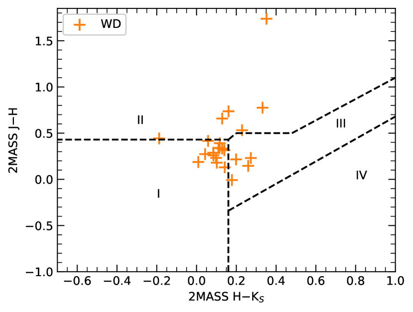
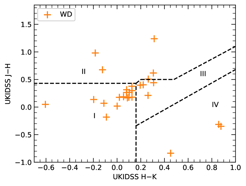
Figure 6: Near-IR (2MASS-top and UKIDSS -bottom) colour-colour diagrams of the hot-WDs selection (orange crosses) are shown. The four regions delimited by a dashed line represent single WD (I), WDs with low-mass, late-type MS star (or L-type star) as a companion (II), WDs with low-mass brown dwarf (L-type star) companion (III), and WDs that are probably contaminated by the presence of circumstellar material (IV) (see Wellhouse et al. 2005).

5.4 Nebulae around the WDs

Finally, we searched for the presence of H$\alpha$ emitting nebulae around the 74 hottest new WD candidates using the IPHAS/IGAPS imagery, and we found no obvious sign of such nebulosities in the close vicinity of the objects in our sample (up to 15$\arcmin$). We note however that the exposure time used for the H$\alpha$ images is relatively short (120s), and as it was shown by Sabin et al. (2021), deeper observations of these IPHAS/IGAPS objects can reveal new faint external structures. Then, in very few cases, we found the WDs candidates embedded in an H$\alpha$ cloud. We also searched for H$\alpha$ excess in these sources using the data by (Fratta et al. 2021). In Table 2, the last column indicates that only 17 out of 74 objects present such excess with a 3$\sigma$ significance. We identified 6 of them as single and 11 in a binary system. In the latter case, the H$\alpha$-excess could be due to accretion onto the WD. Therefore, deeper optical imaging is needed to investigate if the WDs are (still) surrounded by an ionised (planetary) nebula.

6 Conclusions

GALEX UV in combination with optical databases offers a unique opportunity to investigate and characterise WD stars that are usually elusive in the optical range. We combined GALEX UV with the optical IGAPS catalogue and found 74 WD star candidates in the footprint of both catalogues. The selection of the WD candidates was made by analysing the colour-colour diagrams using different combinations of colours (see Figure 2).

An analysis of the SED was done by implementing an MCMC algorithm to fit the GALEX UV and IGAPS photometry resulting in 19 and 31 single and binary WD candidates, respectively (see apendix A and B). The combination of Gaia EDR3 distances enables us to determine the stellar parameters which in turn enable the characterisation of different evolutionary stages. However, for the very hot stars, a small $T_{\rm eff}$ uncertainty, may increase the uncertainty of the reddening calculation and hence affecting the derived evolutionary stage (see Figures 3 and 4). A spectral analysis must be done in order to obtain more accurate values of the hot star stellar parameters and to confirm its single and/or binary nature.

We classified the WD star candidates by analysing the different IR colours using photometric data from 2MASS and UKIDSS catalogues. Objects found to be single and binary WD candidates in the IR colour-colour diagrams (see Figure 6) also resulted as such in the SED analysis. This supports the strength of the method used in Section 4 and the advantages of the combination of GALEX UV with optical photometry. The IR colour-colour diagrams enable us to also identify WD stars that probably contain a brown dwarf or planetary companion. Follow-up TESS observations with higher cadence as well as follow-up using ground-based facilities are required in order to obtain more accurate information on the binary parameters. Finally, no nebulae were detected around the hot-WDs by exploiting the short exposure IGAPS imagery, further deeper observations are needed to unveil the very evolved PNe.

Data Availability

All data used in this manuscript are available through public archives.

Appendix A Single WD fitting

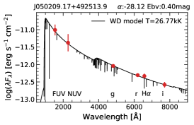
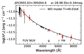
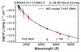
Figure 8: Similar to Figure 7.

Appendix B Binary WD SED fitting

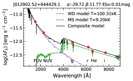
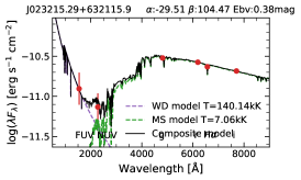
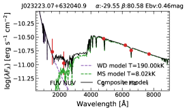
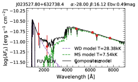
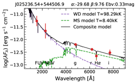
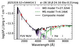
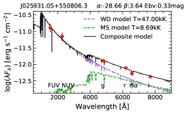
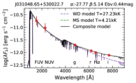
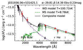
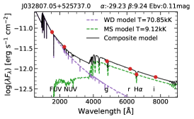
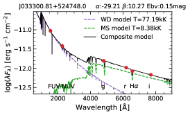
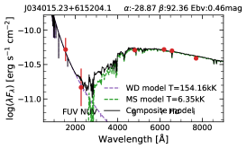
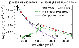
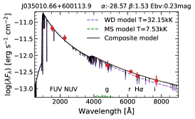
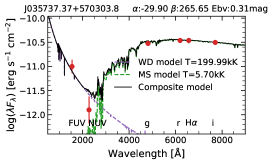
Figure 9: SED fit of the GALEX FUV and NUV + IGAPS g, r, i, and H$\alpha$ photometry (red dots) from which a binary WD star is infered. Synthetic spectra of the best fit of hot and cool star is shown as purple and green dashed lines, respectively. The composite model spectrum is also shown (black solid line).

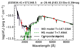
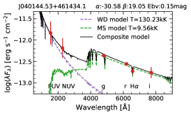
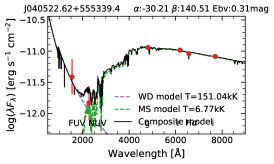
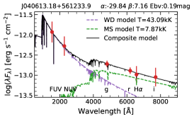
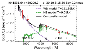
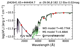
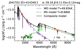
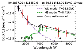
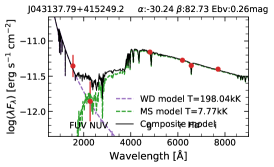
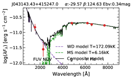
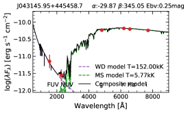
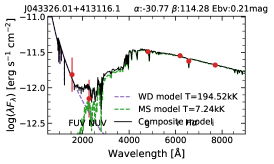
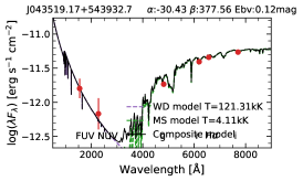
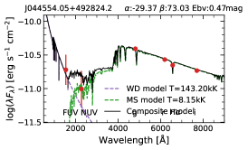
Figure 10: Similar to Figure 9.

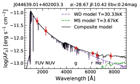
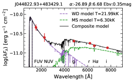
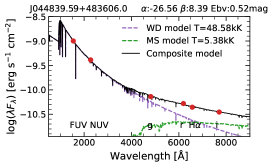
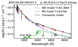
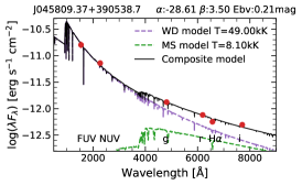
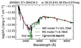
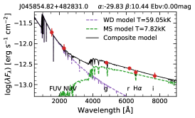
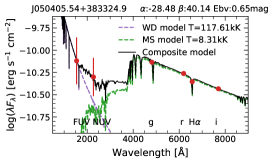
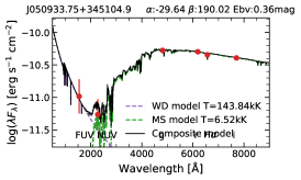
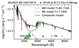
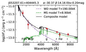
Figure 11: Similar to Figure 9.

References

- Allard et al. (2012) Allard F., Homeier D., Freytag B., 2012, Philosophical Transactions of the Royal Society of London Series A, 370, 2765
- Almaini et al. (2007) Almaini O., et al., 2007, in Metcalfe N., Shanks T., eds, Astronomical Society of the Pacific Conference Series Vol. 379, Cosmic Frontiers. p. 163
- Althaus et al. (2013) Althaus L. G., Miller Bertolami M. M., Córsico A. H., 2013, A&A, 557, A19
- Bailer-Jones et al. (2021) Bailer-Jones C. A. L., Rybizki J., Fouesneau M., Demleitner M., Andrae R., 2021, AJ, 161, 147
- Barentsen et al. (2014) Barentsen G., et al., 2014, MNRAS, 444, 3230
- Barker et al. (2018) Barker H., Zijlstra A., De Marco O., Frew D. J., Drew J. E., Corradi R. L. M., Eislöffel J., Parker Q. A., 2018, MNRAS, 475, 4504
- Bianchi (2009) Bianchi L., 2009, Ap&SS, 320, 11
- Bianchi & Shiao (2020) Bianchi L., Shiao B., 2020, ApJS, 250, 36
- Bianchi et al. (2009) Bianchi L., Hutchings J. B., Efremova B., Herald J. E., Bressan A., Martin C., 2009, AJ, 137, 3761
- Bianchi et al. (2011) Bianchi L., Efremova B., Herald J., Girardi L., Zabot A., Marigo P., Martin C., 2011, MNRAS, 411, 2770
- Bianchi et al. (2017) Bianchi L., Shiao B., Thilker D., 2017, ApJS, 230, 24
- Bianchi et al. (2018) Bianchi L., Keller G. R., Bohlin R., Barstow M., Casewell S., 2018, Ap&SS, 363, 166
- Camisassa et al. (2016) Camisassa M. E., Althaus L. G., Córsico A. H., Vinyoles N., Serenelli A. M., Isern J., Miller Bertolami M. M., García-Berro E., 2016, ApJ, 823, 158
- Camisassa et al. (2019) Camisassa M. E., et al., 2019, A&A, 625, A87
- Capaccioli et al. (2012) Capaccioli M., et al., 2012, in Science from the Next Generation Imaging and Spectroscopic Surveys. p. 1
- Cardelli et al. (1989) Cardelli J. A., Clayton G. C., Mathis J. S., 1989, ApJ, 345, 245
- Castelli & Kurucz (2003) Castelli F., Kurucz R. L., 2003, in Piskunov N., Weiss W. W., Gray D. F., eds, Vol. 210, Modelling of Stellar Atmospheres. p. A20 (arXiv:astro-ph/0405087)
- Choi et al. (2016) Choi J., Dotter A., Conroy C., Cantiello M., Paxton B., Johnson B. D., 2016, ApJ, 823, 102
- De Marco et al. (2013) De Marco O., Passy J.-C., Frew D. J., Moe M., Jacoby G. H., 2013, MNRAS, 428, 2118
- Drew et al. (2014) Drew J. E., et al., 2014, MNRAS, 440, 2036
- Drew et al. (2015) Drew J. E., et al., 2015, VizieR Online Data Catalog, p. J/MNRAS/440/2036
- Feinstein et al. (2019) Feinstein A. D., et al., 2019, PASP, 131, 094502
- Foreman-Mackey et al. (2013) Foreman-Mackey D., Hogg D. W., Lang D., Goodman J., 2013, PASP, 125, 306
- Fratta et al. (2021) Fratta M., et al., 2021, MNRAS, 505, 1135
- Gaia Collaboration (2020) Gaia Collaboration 2020, VizieR Online Data Catalog, p. I/350
- Gaia Collaboration & et al. (2018) Gaia Collaboration et al. 2018, A&A, 616, A1
- Gaia Collaboration et al. (2021) Gaia Collaboration et al., 2021, A&A, 649, A1
- Gentile Fusillo et al. (2019) Gentile Fusillo N. P., et al., 2019, MNRAS, 482, 4570
- Gentile Fusillo et al. (2021) Gentile Fusillo N. P., et al., 2021, MNRAS, 508, 3877
- Green (2018) Green G., 2018, The Journal of Open Source Software, 3, 695
- Green et al. (2019) Green G. M., Schlafly E., Zucker C., Speagle J. S., Finkbeiner D., 2019, ApJ, 887, 93
- Groot et al. (2009) Groot P. J., et al., 2009, MNRAS, 399, 323
- Hauschildt et al. (1999) Hauschildt P. H., Allard F., Baron E., 1999, ApJ, 512, 377
- Hippke et al. (2019) Hippke M., David T. J., Mulders G. D., Heller R., 2019, AJ, 158, 143
- Hubeny & Lanz (1995) Hubeny I., Lanz T., 1995, ApJ, 439, 875
- Jones (2020) Jones D., 2020, Galaxies, 8, 28
- Jones & Boffin (2017) Jones D., Boffin H. M. J., 2017, Nature Astronomy, 1, 0117
- Kepler et al. (2016) Kepler S. O., et al., 2016, MNRAS, 455, 3413
- Kepler et al. (2019) Kepler S. O., et al., 2019, MNRAS, 486, 2169
- Koester (2010) Koester D., 2010, Mem. Soc. Astron. Italiana, 81, 921
- Koester & Chanmugam (1990) Koester D., Chanmugam G., 1990, Reports on Progress in Physics, 53, 837
- Kovács et al. (2002) Kovács G., Zucker S., Mazeh T., 2002, A&A, 391, 369
- Kuijken et al. (2002) Kuijken K., et al., 2002, The Messenger, 110, 15
- Kwitter & Henry (2022) Kwitter K. B., Henry R. B. C., 2022, PASP, 134, 022001
- Lawrence et al. (2007) Lawrence A., et al., 2007, MNRAS, 379, 1599
- Martin et al. (2005) Martin D. C., et al., 2005, ApJ, 619, L1
- Miller Bertolami (2016) Miller Bertolami M. M., 2016, A&A, 588, A25
- Monguió et al. (2020) Monguió M., et al., 2020, A&A, 638, A18
- Morrissey et al. (2007) Morrissey P., et al., 2007, ApJS, 173, 682
- Osuna et al. (2008) Osuna P., et al., 2008, IVOA Astronomical Data Query Language Version 2.00, IVOA Recommendation 30 October 2008 (arXiv:1110.0503), doi:10.5479/ADS/bib/2008ivoa.spec.1030O
- Panei et al. (2007) Panei J. A., Althaus L. G., Chen X., Han Z., 2007, MNRAS, 382, 779
- Parker et al. (2005) Parker Q. A., et al., 2005, MNRAS, 362, 689
- Parker et al. (2006) Parker Q. A., et al., 2006, MNRAS, 373, 79
- Raddi et al. (2017) Raddi R., et al., 2017, MNRAS, 472, 4173
- Raghavan et al. (2010) Raghavan D., et al., 2010, ApJS, 190, 1
- Ricker et al. (2015) Ricker G. R., et al., 2015, Journal of Astronomical Telescopes, Instruments, and Systems, 1, 014003
- Sabin et al. (2014) Sabin L., et al., 2014, MNRAS, 443, 3388
- Sabin et al. (2021) Sabin L., et al., 2021, arXiv e-prints, p. arXiv:2108.13612
- Schlegel et al. (1998) Schlegel D. J., Finkbeiner D. P., Davis M., 1998, ApJ, 500, 525
- Skrutskie et al. (2006) Skrutskie M. F., et al., 2006, AJ, 131, 1163
- Stassun et al. (2018) Stassun K. G., et al., 2018, AJ, 156, 102
- Vanderburg et al. (2020) Vanderburg A., et al., 2020, Nature, 585, 363
- Weidmann et al. (2020) Weidmann W. A., et al., 2020, A&A, 640, A10
- Wellhouse et al. (2005) Wellhouse J. W., Hoard D. W., Howell S. B., Wachter S., Esin A. A., 2005, PASP, 117, 1378
- Winters et al. (2019) Winters J. G., et al., 2019, AJ, 157, 216
- York et al. (2000) York D. G., et al., 2000, AJ, 120, 1579