The Fredkin staircase: An integrable system with a finite-frequency Drude peak

Abstract

We introduce and explore an interacting integrable cellular automaton, the Fredkin staircase, that lies outside the existing classification of such automata, and has a structure that seems to lie beyond that of any existing Bethe-solvable model. The Fredkin staircase has two families of ballistically propagating quasiparticles, each with infinitely many species. Despite the presence of ballistic quasiparticles, charge transport is diffusive in the d.c. limit, albeit with a highly non-gaussian dynamic structure factor. Remarkably, this model exhibits persistent temporal oscillations of the current, leading to a delta-function singularity (Drude peak) in the a.c. conductivity at nonzero frequency. We analytically construct an extensive set of operators that anticommute with the time-evolution operator; the existence of these operators both demonstrates the integrability of the model and allows us to lower-bound the weight of this finite-frequency singularity.

Introduction— Conventional hydrodynamics predicts that high-temperature transport in lattice systems should generically be diffusive. This expectation is strongly violated in two tractable classes of systems. First, kinetically constrained models (KCMs)—i.e., models of stochastic dynamics subject to hard kinetic constraints, initially introduced as toy models of glassy behavior Garrahan (2018); Fredrickson and Anderson (1984); Garrahan et al. (2010); Ritort and Sollich (2003); Everest et al. (2016)—have been shown to exhibit subdiffusive transport under quite general conditions. In some subdiffusive KCMs the constraints lead to the presence of additional conservation laws, giving rise to “fracton hydrodynamics” Iaconis et al. (2019); Feldmeier et al. (2020); Gromov et al. (2020); Morningstar et al. (2020); in other cases, it is unclear whether additional conservation laws are present Singh et al. (2021); Richter and Pal (2022). Subdiffusion in KCMs was experimentally observed in Ref. Guardado-Sanchez et al. (2020). A second class of systems that escape conventional hydrodynamics are integrable systems Castro-Alvaredo et al. (2016); Bertini et al. (2016); Bulchandani et al. (2017); Bastianello et al. (2022), which have extensively many conservation laws, as well as stable ballistically propagating quasiparticles. One might expect transport in integrable systems to be ballistic, but in the presence of internal symmetries, integrable spin chains can exhibit transport that is sub-ballistic, and either diffusive or superdiffusive De Nardis et al. (2018); Gopalakrishnan et al. (2018); Gopalakrishnan and Vasseur (2019); Nardis et al. (2019); Bulchandani et al. (2021). Remarkably, there are deep links between integrable systems and KCMs: if one applies the update rules of a KCM in certain deterministic sequences (rather than at random) one obtains discrete-time integrable cellular automata. This correspondence has been noted in multiple cases, see e.g. Medenjak et al. (2017); Gopalakrishnan (2018); Gopalakrishnan and Zakirov (2018); Friedman et al. (2019); Buča et al. (2021); Pozsgay (2021); Gombor and Pozsgay (2021, 2022); how general it is, and how the properties of the stochastic and integrable versions of the model are related, remain open questions.

In the present work we identify a new such correspondence, by constructing an integrable cellular automaton based on the Fredkin update rule. This update rule acts on four adjacent sites, swapping the middle two provided the outer sites obey the kinetic constraint sketched in Fig. 1. The stochastic Fredkin model Singh et al. (2021); Causer et al. (2022) has nontrivial subdiffusive dynamics, with a spacetime scaling $x\sim t^{3/8}$ whose origin is not yet understood. We construct a cellular automaton with the Fredkin update rule; we call this model the Fredkin staircase automaton (FSA). We show that the FSA is integrable by explicitly showing how an extensive family of conservation laws can be constructed; however, we have not completely solved the model as the conservation laws we construct do not exhaust its quasiparticle content. Because the FSA is a cellular automaton, we are able to extract both the spectrum of quasiparticles and scattering phase shifts between them from numerics. We find two families of quasiparticle species, called $\beta$ and $\sigma$ quasiparticles. The $\beta$ quasiparticles also form bound states, which we call $\beta$-strings; there is an infinite family of these. The scattering properties between $\beta$ and $\sigma$ quasiparticles are unusual, and it is not clear how to relate the integrable structures we find to standard Bethe ansatz concepts.

In addition to identifying the quasiparticle structure, we study transport in this model by numerically computing its a.c. conductivity through the Kubo formula Bertini et al. (2021). Our most unexpected finding is that the a.c. conductivity has a $\delta$-function “Drude” peak at a nonzero frequency, associated with persistent oscillations of current fluctuations. We are unaware of any other integrable systems with a nonzero-frequency Drude peak (although related oscillations have been observed in non-hydrodynamic quantities Medenjak et al. (2020)). On the other hand, the d.c. limit of the conductivity is finite, so transport is asymptotically diffusive despite the presence of ballistic quasiparticles. In addition, the dynamical structure factor of this model is spatially strongly asymmetric, and obeys a scaling form $C(x,t)=t^{-1/z}f(x/t^{1/z})$, with $z=2$ and $f$ a skewed, non-Gaussian scaling function. We discuss the origin of these transport phenomena in terms of an infinite family of charges that anti-commute with the time evolution operator.

Model.— Our system is a one dimensional chain of qubits of length $L$ whose basis states we represent as $|\bullet\rangle$ and $|\circ\rangle$ to denote whether a particle has occupied a site or not. The dynamics is governed by a Floquet operator $\mathcal{U}$, shown pictorially in Fig. 1, which is composed of three layers of four site unitary gates, i.e. $\mathcal{U}=V_{3}V_{2}V_{1}$, where

$$V_{i}=\prod_{j\equiv i\,\text{mod}\,3}U_{j,j+1,j+2,j+3},$$ (1)

and

$$\begin{split}U_{j,j+1,j+2,j+3}&=P^{\bullet}_{j}\text{SWAP}_{j+1,j+2}P^{\bullet}\\ &+P^{\bullet}_{j}\text{SWAP}_{j+1,j+2}P^{\circ}_{j+3}\\ &+P^{\circ}_{j}\text{SWAP}_{j+1,j+2}P^{\circ}_{j+3}\\ &+P^{\circ}_{j}\mathds{1}_{j+1,j+2}P^{\bullet}_{j+3}.\end{split}$$ (2)

$P^{\bullet}_{j}=|\bullet\rangle\langle\bullet|_{j}$, $P^{\circ}_{j}=|\circ\rangle\langle\circ|_{j}$ and $\text{SWAP}_{j,j+1}$ is the usual swap gate. Note that these gates locally preserve particle number so that the total particle number of the system is conserved.

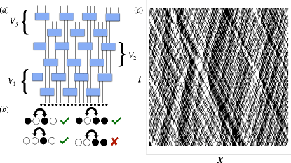
Figure 1: Model. (a) Pictorial representation of the circuit geometry described by Eq.1. (b) Pictorial representation of the rules associated to the Fredkin constraint as described in Eq.2. $\bullet$ represents particles while $\circ$ represents holes. (c) Time evolution of a random product state in the occupation basis.

We remark that the gate geometry is equivalent to a staircase geometry hence the name: Fredkin Staircase Automaton, as the constrained swaps satisfy the so-called Fredkin constraint Dell’Anna et al. (2016); Chen et al. (2017a, b); Adhikari and Beach (2021); Udagawa and Katsura (2017); Zhang and Klich (2017); Salberger and Korepin (2016); Chen et al. (2020); Movassagh and Shor (2016); Salberger et al. (2017); Langlett and Xu (2021). The gate geometry leads to an asymmetric circuit light-cone for local operators where the support of the light cone increase by 6 sites to the left and 3 sites to the right. Owing to the fact that the circuit light cone increases by a multiple of 3, we will partition our chain into unit cells containing 3 sites. We note that the gate pattern we are using is crucial for the model to be integrable. In the supplemental material SM , we show that deforming the gate geometry breaks the integrability of the model and leads to subdiffusion with an exponent $z\simeq 8/3$ in line with the predictions of Ref. Singh et al. (2021). Each update conserves the total number of $\bullet$ (and $\circ$) sites, so we can regard the fraction of $\bullet$ sites as the “filling fraction” $f$.

Quasiparticles.— We first identify single quasiparticle excitations of the FSA model above its vacuum state (i.e., the state $|\circ\rangle^{\otimes N}$). One can create states with a single elementary quasiparticle by occupying a single site. Since there are three inequivalent sites in the unit cell there are three inequivalent quasiparticles. For the gate pattern and unit cell in Fig. 1, quasiparticles on the first and third sites of the unit cell move ballistically leftward with velocity $v_{\sigma}=3/2$, whereas those on the second site move rightward with velocity $v_{\beta}=3$—as this notation anticipates we will call the two left-moving quasiparticles $\sigma$-particles and the right-moving quasiparticle a $\beta$-quasiparticle. (We will avoid calling them left- and right-movers as the direction they move is set by the arbitrarily chosen chirality of the gate pattern.)

We now turn to states with two occupied sites. When the occupied sites are more than one unit cell apart, such states have two quasiparticles, with flavors that depend on the location of the filled site in the unit cell (as above). When the occupied sites are in the same or adjacent unit cells, the identification is more subtle. One might have expected that a configuration like $\bullet\circ\bullet\circ\circ\circ$ or $\circ\circ\bullet\bullet\circ\circ$ contains two $\sigma$-quasiparticles; in fact they contain a $\sigma$ and a $\beta$ quasiparticle in the process of colliding. In this sense, $\sigma$-quasiparticles obey a hardcore constraint: if one slot is occupied its neighbor cannot be. Moreover, as we will see below, two $\beta$-quasiparticles in adjacent unit cells are not independently propagating, but instead form a bound state.

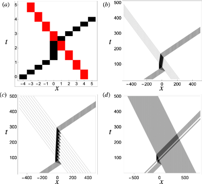
Figure 2: Quasiparticles scattering. (a) A collision between a $\sigma$ (colored red) and $\beta$ (colored black) particle where integer time steps represent evolving by a full Floquet step while fractional steps indicate evolving by individual layers. One can see the $\sigma$ particle receives no scattering shift but the $\beta$ particle is delayed by one Floquet time step. (b) A size 40 $\beta$-string (moving right) collides with a size 200 2-spaced type-A $\sigma$-string (moving left). One can clearly see that the velocity of the $\beta$-string is renormalized when it is inside the $\sigma$-string. (c) A size 40 $\beta$-string collides with a size 200 10-spaced type-A $\sigma$-string. Observe that the the $\beta$-string’s velocity is much lower than compared to the previous situation indicating that the effective velocity of $\beta$-strings is highly dependent on spacings of $\sigma$-particles . (d) Two $\beta$ strings collide when they encounter the large $\sigma$-string. One can see that the smaller $\beta$-string overtakes the larger one after the collision occurs.

We now turn to the scattering between quasiparticles. Here, in contrast to standard integrable systems, we find a strong asymmetry between $\sigma$ and $\beta$ quasiparticles: the trajectories of $\sigma$ quasiparticles are totally unaffected by collisions, while $\beta$ quasiparticles are slowed down. When colliding with a single $\sigma$ quasiparticle, a sequence of $s$ $\beta$ quasiparticles is slowed down by $s$ unit cells. These sequences thus form collectively moving bound states, which we call $\beta$-strings of size $s$; collisions with $\sigma$ quasiparticles renormalize the velocities of such $\beta$-strings in an $s$-dependent way. Lastly, we note that because $\beta$-strings of different sizes have different renormalized velocities (in the presence of $\sigma$ strings), two $\beta$-strings can collide (when a smaller string tries to overtake a larger one). In the bottom-right panel of Fig. 2, we show a collision between a size 40 $\beta$-string and size 10 $\beta$-string. The two collide with each other once they encounter the $\sigma$-string and then one observes that the smaller $\beta$-string “overtakes” the larger $\beta$-string. When two $\beta$-strings of size $(s,s^{\prime})$ collide the faster of them is further sped up (and the slower is further slowed down) by $2\min(s,s^{\prime})$ unit cells. This scattering phase shift precisely parallels the result for Heisenberg spin chains.

To set up generalized hydrodynamics for this model, we would need the scattering shifts between an arbitrary-size $\beta$-string and an arbitrary configuration of $\sigma$ quasiparticles. In a typical Bethe-ansatz solvable problem, one would have to identify all the distinct $\sigma$-type strings and the scattering shift accumulated by a $\beta$-string passing through the $\sigma$ quasiparticles would be a sum of shifts due to each $\sigma$-type string. In the FSA this separation does not happen: rather, the scattering shift is sensitive to the separation between $\sigma$ quasiparticles (Fig. 2). Consider, as a simple example, the case of a $\beta$-string of size $\ell$ scattering off two $\sigma$ quasiparticles separated by $d$ unit cells: the resulting scattering shift is $\min(2\ell,\ell+2d)$ unit cells. Thus, from the point of view of their scattering properties, even two arbitrarily well separated $\sigma$ quasiparticles cannot be treated as independent scatterers with additive scattering shifts. Although we are able to find expressions for the scattering shift of an arbitrary $\beta$-string in an arbitrary background of $\sigma$ quasiparticles, it is not clear how to express these in the standard Bethe ansatz form. Nevertheless, our numerical results strongly suggest that all quasiparticles are stable (so the model is integrable), and we now explicitly demonstrate this for the $\sigma$ quasiparticles.

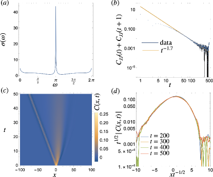
Figure 3: Transport. (a) a.c. conductivity $\sigma(\omega)$. Note that $\omega=\pi$ features a prominent peak indicating a $\pi$ Drude weight and that we also have a finite non-zero value at $\omega=0$ which suggests diffusive behavior. (b) Behavior of the Kubo correlator $C_{JJ}(t)+C_{JJ}(t+1)$ which is twice the average value over one period of the oscillations in the current-current correlator. $C_{JJ}(t)+C_{JJ}(t+1)$ falls off in a power law fashion, i.e. $t^{-\beta}$, with $\beta\approx 1.7>1$ indicating the presence of a finite non-zero diffusion constant at low frequency. (c) Behavior of the particle structure factor $C(x,t)$ at short times and (d) Diffusive scaling collapse of the structure factor, $C(x,t)=t^{-1/2}f(x/t^{1/2})$ with $f$ a non-Gaussian skewed scaling function. (a) and (b) is data averaged over $10^{8}$ realizations and (c) and (d) are averaged over $10^{7}$ realizations.

Integrability.— In this section we show that there are an infinite number of quasi-local operators that are conserved. The construction is based on the intuition that operators which correspond to creating $\sigma$-strings should be rather simple to construct since $\sigma$-strings propagate without scattering delays. First, we note that a $\sigma$-particle is given by the one of the following configurations: $\bullet\square\circ$ or $\square\square\bullet\circ\square\square$, where $\square$ is meant to denote that a particle may or may not occupy that site. Using the above fact, one can construct a number operator counting the total number of $\sigma$-particles spaced by $s$ unit cells given by

$$N_{s}=N_{s}^{\bullet\times\circ}+N_{s}^{\bullet\circ},$$ (3)

where

$$N_{s}^{\bullet\times\circ} =\sum_{i\equiv 1\text{mod}3}P^{\bullet\times\circ}_{i}\prod_{j=i+1}^{i+s}(\mathds{1}-P_{j}^{\bullet\times\circ})P^{\bullet\times\circ}_{i+s+1},$$ (4)

$$N_{s}^{\bullet\circ} =\sum_{i\equiv 1\text{mod}3}P^{\bullet}_{i-1}P^{\circ}_{i}\prod_{j=i+1}^{i+s}(\mathds{1}-P_{j-1}^{\bullet}P_{j}^{\circ})P_{i+s}^{\bullet}P_{i+s+1}^{\circ},$$

is conserved. If $s\leq 0$ one should replace the product of operators with an identity operator and we note that for $s=-1$, $N_{s}$ simply counts the total number of $\sigma$-particles. We further note that the $N_{s}^{\bullet\times\circ}$ and $N_{s}^{\bullet\circ}$ correspond to the asymptotic spacings Gopalakrishnan et al. (2018) of type-A and type-B $\sigma$-particles, respectively.

One can show that $N_{s}$ is conserved by noting that the Floquet evolution operator, $\mathcal{U}$, maps $P_{i}^{\bullet\times\circ}\mapsto P_{i-1}^{\bullet}P_{i}^{\circ}$ and $P_{i-1}^{\bullet}P_{i}^{\circ}\mapsto P_{i-3}^{\bullet\times\circ}$ which implies $N_{s}^{\bullet\times\circ}\leftrightarrow N_{s}^{\bullet\circ}$ at each time step.

All operators commute with each other since they are diagonal in the occupation basis. Additionally, they are orthogonal to each other under the Hilbert-Schmidt inner product (i.e., $\langle A,B\rangle\equiv 2^{-L}\langle A^{\dagger}B\rangle$) because for $s^{\prime}>s$, all terms in $N_{s^{\prime}}$ have larger support than all terms in $N_{s}$. Since we constructed an infinite set of linearly independent conserved quasi-local operators, the FSA model is integrable. We note that there are clearly more operators which are conserved such as the total number of $\beta$-strings. It would be interesting to further investigate the algebraic integrable structure of this model in future work Gombor and Pozsgay (2021); Pozsgay (2021); Prosen (2021); Gombor and Pozsgay (2022); Buča et al. (2021); Gombor and Pozsgay (2022).

Transport.— Because of its integrability, it is natural to expect particle transport in the FSA model to be ballistic: if the particle current overlaps with any of the conserved charges, it cannot fully relax leading to persistent currents. In what follows, we argue analytically and numerically that transport in the FSA is a lot more exotic and interesting: none of the charges uncovered above overlap with the current operator, and we find numerically that low frequency transport is diffusive. However, we identify analytically another set of changes which anticommute with the time evolution operator, and which do have a finite overlap with the current. We argue that this leads to a finite Drude peak in the conductivity at frequency $\omega=\pi$. Alternatively, it shows that the FSA is a (fine-tuned) equilibrium discrete time-crystal Khemani et al. (2016); Else et al. (2016); Khemani et al. (2019); Medenjak et al. (2020), as it exhibits persistent oscillating currents.

We characterize the transport properties of the FSA by computing the current-current correlation function, $C_{JJ}(t)=\frac{1}{L}\langle J(t)J(0)\rangle$, where $J(t)=\sum_{x}j(x,t)$ and $j(x,t)$ represents the local current density and $\langle A\rangle\equiv 2^{-L}\text{tr}(A)$ for an operator $A$. We present the details of the calculation of $j(x,t)$ and its lengthy expression in the supplemental material SM . We numerically computed $C_{JJ}(t)$ using classical evolution and averages are performed over $10^{8}$ random initial states.

From the current-current correlator, we compute the a.c. conductivity, $\sigma(\omega)$ by using the Kubo formula Bertini et al. (2021)

$$\sigma(\omega)=\frac{1}{2}C_{JJ}(t=0)+\sum_{t=1}^{\infty}{\rm e}^{i\omega t}C_{JJ}(t).$$ (5)

Because of the Floquet (discrete time) nature of model, we have $\omega\in[0,2\pi)$. We computed this conductivity numerically, see Fig. 3. One can see a clear peak at $\omega=\pi$ indicating persistent oscillations in the time-dependent conductivity and hence also the current-current correlator. We attribute these persistent oscillations to the existence of an extensive number of operators $Q$ such that $\mathcal{U}^{\dagger}Q\mathcal{U}=-Q$. To see that such operators imply such persistent oscillations , consider the $\pi$-Drude weight, defined as

$$\mathcal{D}_{\pi}=\lim_{t\rightarrow\infty}\frac{1}{t}\sum_{\tau=1}^{t}(-1)^{\tau}C_{JJ}(\tau).$$ (6)

The $\pi$-Drude weight characterizes the weight of a possible Drude (delta function) peak in the conductivity at frequency $\pi$.

One can show that if a collection of operators $Q_{s}$ satisfy the aforementioned conditions then one can lower bound $\mathcal{D}_{\pi}$ through the application of a Mazur bound Mazur (1969); Dhar et al. (2021); Ampelogiannis and Doyon (2021), i.e.

$$\mathcal{D}_{\pi}\geq\frac{3}{L}\sum_{s}\frac{\langle J(0)Q_{s}\rangle^{2}}{\langle Q_{s}^{2}\rangle}.$$ (7)

A family of such operators $Q_{s}$ are given by $Q_{s}=N_{s}^{\bullet\times\circ}-N_{s}^{\bullet\circ}$ and they anticommute with $\mathcal{U}$ since $N_{s}^{\bullet\times\circ}\leftrightarrow N_{s}^{\bullet\circ}$ at each time step:

$$\{Q_{s},\mathcal{U}\}=0$$ (8)

We remark that if these were all the charges which anticommuted with $\mathcal{U}$ then Eq. 7 would become an equality. The fact that $\langle J(0)Q_{s}\rangle\neq 0$ means that $\mathcal{D}_{\pi}$ is non-zero which implies that $C_{JJ}(t)$ necessarily has to be of the form $C_{JJ}(t)=(-1)^{t}(\mathcal{D}_{\pi}+\text{sub-leading terms})$. Such persistent oscillations indicate that the FSA is a discrete time crystal—albeit fine-tuned rather than generic Khemani et al. (2016); Else et al. (2016); Khemani et al. (2019); Buča (2022); Medenjak et al. (2020).

Despite this exotic behavior near $\omega=\pi$ frequency, low-frequency transport appears to be diffusive. None of the charges (4) overlap the current, so there is no obvious zero-frequency Drude weight. Numerically, we find that the averaged Kubo correlators $C_{JJ}(t)+C_{JJ}(t+1)$ decays as $t^{-\beta}$, with an exponent $\beta\approx 1.7>1$, indicating a finite d.c. conductivity $\sigma(\omega=0)$, and thus a finite diffusion constant. The structure factor $C(x,t)=\langle q(x,t)q(0,0)\rangle$, with $q$ the local particle number appropriately coarse-grained over unit cells SM , displays an ever richer structure (Fig. 3), with some ballistic peak carrying vanishing weight due to $\sigma$-strings, and an asymmetric non-Gaussian diffusive peak near the origin.

Discussion.—In this work we introduced a new reversible cellular automaton based on the Fredkin update rule. We showed that the spectrum of this automaton contains two genera of stable quasiparticles, the $\beta$-strings and the $\sigma$ quasiparticles. The $\beta$-strings of all sizes have the same bare velocity, but are renormalized differently through their collisions with $\sigma$ quasiparticles. Thus this model features an infinite hierarchy of quasiparticles with distinct effective velocities above a typical thermal state. The motion of the $\sigma$ quasiparticles, meanwhile, is unaffected by the scattering, so it is not entirely clear if (and how) one can assign them to “strings.” As we discussed, the $\beta-\sigma$ scattering depends nontrivially on the spacing between adjacent $\sigma$ quasiparticles; while this dependence can be computed, we have not been able to factor it into contributions due to a hierarchy of $\sigma$-type strings. Thus the full Bethe ansatz solution of this model remains a task for future work. We remark that this model does not appear to fall under a current partial classification of integrable CAs Gombor and Pozsgay (2021); Pozsgay .

Although we were unable to fully solve the model, we could analytically establish the presence of an infinite hierarchy of conserved charges; physically, these charges represent the spacings between $\sigma$ quasiparticles, which are conserved. Such asymptotic spacings are also conserved in the Rule 54 RCA Gopalakrishnan (2018); Buča et al. (2021) but do not seem to affect the hydrodynamics of the model. However, scattering of $\beta$ strings depends on spacings of $\sigma$-particles in a $\sigma$-string suggesting that they might play a role in determining the late time behavior of the FSA.

Finally, we studied transport properties in this model. We found that the d.c. limit of transport is diffusive, but with an asymmetric and non-gaussian dynamic structure factor. Moreover, the model features persistent current oscillations, leading to a finite-frequency delta-function peak in the a.c. conductivity. A comprehensive understanding of the transport behavior in this model should be amenable to generalized hydrodynamics (GHD) Bastianello et al. (2022). However, this would require one to re-express the scattering data in a standard Bethe-ansatz form; this task is currently out of reach.

Acknowledgements.— We thank B. Pozsgay and B. Ware for stimulating discussions. This work was supported by the National Science Foundation under NSF Grant No. DMR-1653271 (S.G.), the US Department of Energy, Office of Science, Basic Energy Sciences, under Early Career Award No. DE-SC0019168 (R.V.), and the Alfred P. Sloan Foundation through a Sloan Research Fellowship (R.V.).

See pages 1 of suppmat.pdf

See pages 2 of suppmat.pdf

See pages 3 of suppmat.pdf

See pages 4 of suppmat.pdf

See pages 5 of suppmat.pdf

See pages 6 of suppmat.pdf

See pages 7 of suppmat.pdf

See pages 8 of suppmat.pdf

See pages 9 of suppmat.pdf

See pages 10 of suppmat.pdf

References

- Garrahan (2018) J. P. Garrahan, Physica A: Statistical Mechanics and its Applications 504, 130 (2018), lecture Notes of the 14th International Summer School on Fundamental Problems in Statistical Physics.
- Fredrickson and Anderson (1984) G. H. Fredrickson and H. C. Anderson, Physical Review Letters 53, 1244 (1984).
- Garrahan et al. (2010) J. P. Garrahan, P. Sollich, and C. Toninelli, “Kinetically constrained models,” (2010).
- Ritort and Sollich (2003) F. Ritort and P. Sollich, Advances in Physics 52, 219 (2003).
- Everest et al. (2016) B. Everest, M. Marcuzzi, J. Garrahan, and I. Lesanovsky, Physical Review E 94 (2016), 10.1103/PhysRevE.94.052108.
- Iaconis et al. (2019) J. Iaconis, S. Vijay, and R. Nandkishore, Physical Review B 100 (2019), 10.1103/PhysRevB.100.214301.
- Feldmeier et al. (2020) J. Feldmeier, P. Sala, G. D. Tomasi, F. Pollmann, and M. Knapp, Physical Review Letters 125 (2020), 10.1103/PhysRevLett.125.245303.
- Gromov et al. (2020) A. Gromov, A. Lucas, and R. Nandkishore, Physical Review Research 2 (2020), 10.1103/PhysRevResearch.2.033124.
- Morningstar et al. (2020) A. Morningstar, V. Khemani, and D. A. Huse, Physical Review B 101 (2020), 10.1103/PhysRevB.101.214205.
- Singh et al. (2021) H. Singh, B. A. Ware, R. Vasseur, and A. J. Friedman, Physical Review Letters 127 (2021), 10.1103/PhysRevLett.127.230602.
- Richter and Pal (2022) J. Richter and A. Pal, Physical Review Research 4 (2022), 10.1103/PhysRevResearch.4.L012003.
- Guardado-Sanchez et al. (2020) E. Guardado-Sanchez, A. Morningstar, B. M. Spar, P. T. Brown, D. A. Huse, and W. S. Bakr, Phys. Rev. X 10, 011042 (2020).
- Castro-Alvaredo et al. (2016) O. A. Castro-Alvaredo, B. Doyon, and T. Yoshimura, Phys. Rev. X 6, 041065 (2016).
- Bertini et al. (2016) B. Bertini, M. Collura, J. De Nardis, and M. Fagotti, Phys. Rev. Lett. 117, 207201 (2016).
- Bulchandani et al. (2017) V. B. Bulchandani, R. Vasseur, C. Karrasch, and J. E. Moore, Phys. Rev. Lett. 119, 220604 (2017).
- Bastianello et al. (2022) A. Bastianello, B. Bertini, B. Doyon, and R. Vasseur, Journal of Statistical Mechanics: Theory and Experiment 2022, 014001 (2022).
- De Nardis et al. (2018) J. De Nardis, D. Bernard, and B. Doyon, Phys. Rev. Lett. 121, 160603 (2018).
- Gopalakrishnan et al. (2018) S. Gopalakrishnan, D. A. Huse, V. Khemani, and R. Vasseur, Physical Review B 98 (2018), 10.1103/PhysRevB.98.220303.
- Gopalakrishnan and Vasseur (2019) S. Gopalakrishnan and R. Vasseur, Phys. Rev. Lett. 122, 127202 (2019).
- Nardis et al. (2019) J. D. Nardis, D. Bernard, and B. Doyon, SciPost Phys. 6, 49 (2019).
- Bulchandani et al. (2021) V. B. Bulchandani, S. Gopalakrishnan, and E. Ilievski, Journal of Statistical Mechanics: Theory and Experiment 2021, 084001 (2021).
- Medenjak et al. (2017) M. Medenjak, K. Klobas, and T. Prosen, Physical Review Letters 119 (2017), 10.1103/PhysRevLett.119.110603.
- Gopalakrishnan (2018) S. Gopalakrishnan, Physical Review B 98 (2018), 10.1103/PhysRevB.98.060302.
- Gopalakrishnan and Zakirov (2018) S. Gopalakrishnan and B. Zakirov, Quantum Science and Technology 3, 044004 (2018).
- Friedman et al. (2019) A. J. Friedman, S. Gopalakrishnan, and R. Vasseur, Phys. Rev. Lett. 123, 170603 (2019).
- Buča et al. (2021) B. Buča, K. Klobas, and T. Prosen, Journal of Statistical Mechanics: Theory and Experiment 2021, 074001 (2021).
- Pozsgay (2021) B. Pozsgay, Journal of Physics A: Mathematical and Theoretical 54, 384001 (2021).
- Gombor and Pozsgay (2021) T. Gombor and B. Pozsgay, Phys. Rev. E 104, 054123 (2021).
- Gombor and Pozsgay (2022) T. Gombor and B. Pozsgay, SciPost Phys. 12, 102 (2022).
- Causer et al. (2022) L. Causer, J. P. Garrahan, and A. Lamacraft, “Slow dynamics and large deviations in classical stochastic fredkin chains,” (2022), arXiv:2202.06989 [cond-mat.stat-mech] .
- Bertini et al. (2021) B. Bertini, F. Heidrich-Meisner, C. Karrasch, T.Prosen, R. Steinigeweg, and M. Žnidarič, Reviews of Modern Physics 93 (2021), 10.1103/RevModPhys.93.025003.
- Medenjak et al. (2020) M. Medenjak, B. Buča, and D. Jaksch, Phys. Rev. B 102, 041117 (2020).
- Dell’Anna et al. (2016) L. Dell’Anna, O. Salberger, L. Barbiero, A. Trombettoni, and V. E. Korepin, Phys. Rev. B 94, 155140 (2016).
- Chen et al. (2017a) X. Chen, E. Fradkin, and W. Witczak-Krempa, Journal of Physics A: Mathematical and Theoretical 50, 464002 (2017a).
- Chen et al. (2017b) X. Chen, E. Fradkin, and W. Witczak-Krempa, Physical Review B 96 (2017b), 10.1103/PhysRevB.96.180402.
- Adhikari and Beach (2021) K. Adhikari and K. S. D. Beach, Phys. Rev. B 104, 115149 (2021).
- Udagawa and Katsura (2017) T. Udagawa and H. Katsura, Journal of Physics A: Mathematical and Theoretical 50, 405002 (2017).
- Zhang and Klich (2017) Z. Zhang and I. Klich, Journal of Physics A: Mathematical and Theoretical 50, 425201 (2017).
- Salberger and Korepin (2016) O. Salberger and V. Korepin, “Fredkin spin chain,” (2016).
- Chen et al. (2020) X. Chen, R. Nandkishore, and A. Lucas, Physical Review B 101 (2020), 10.1103/PhysRevB.101.064307.
- Movassagh and Shor (2016) R. Movassagh and P. W. Shor, Proceedings of the National Academy of Sciences 113, 13278 (2016).
- Salberger et al. (2017) O. Salberger, T. Udagawa, Z. Zhang, H. Katsura, I. Klich, and V. Korepin, Journal of Statistical Mechanics: Theory and Experiment 2017, 063103 (2017).
- Langlett and Xu (2021) C. M. Langlett and S. Xu, Physical Review B 103 (2021), 10.1103/PhysRevB.103.L220304.
- (44) See supplemental material .
- Prosen (2021) T. Prosen, arXiv e-prints , arXiv:2106.01292 (2021), arXiv:2106.01292 [cond-mat.stat-mech] .
- Gombor and Pozsgay (2022) T. Gombor and B. Pozsgay, arXiv e-prints , arXiv:2205.02038 (2022), arXiv:2205.02038 [nlin.SI] .
- Khemani et al. (2016) V. Khemani, A. Lazarides, R. Moessner, and S. Sondhi, Physical Review Letters 116 (2016), 10.1103/PhysRevLett.116.250401.
- Else et al. (2016) D. V. Else, B. Bauer, and C. Nayak, Phys. Rev. Lett. 117, 090402 (2016).
- Khemani et al. (2019) V. Khemani, R. Moessner, and S. L. Sondhi, arXiv e-prints , arXiv:1910.10745 (2019), arXiv:1910.10745 [cond-mat.str-el] .
- Mazur (1969) P. Mazur, Physica 43, 533 (1969).
- Dhar et al. (2021) A. Dhar, A. Kundu, and K. Saito, Chaos, Solitons and Fractals 144, 110618 (2021).
- Ampelogiannis and Doyon (2021) D. Ampelogiannis and B. Doyon, “Ergodicity and hydrodynamic projections in quantum spin lattices at all frequencies and wavelengths,” (2021).
- Buča (2022) B. Buča, Phys. Rev. Lett. 128, 100601 (2022).
- (54) B. Pozsgay, Private communication .