Disentangling Visual Embeddings for Attributes and Objects

Abstract

We study the problem of compositional zero-shot learning for object-attribute recognition. Prior works use visual features extracted with a backbone network, pre-trained for object classification and thus do not capture the subtly distinct features associated with attributes. To overcome this challenge, these studies employ supervision from the linguistic space, and use pre-trained word embeddings to better separate and compose attribute-object pairs for recognition. Analogous to linguistic embedding space, which already has unique and agnostic embeddings for object and attribute, we shift the focus back to the visual space and propose a novel architecture that can disentangle attribute and object features in the visual space. We use visual decomposed features to hallucinate embeddings that are representative for the seen and novel compositions to better regularize the learning of our model. Extensive experiments show that our method outperforms existing work with significant margin on three datasets: MIT-States, UT-Zappos, and a new benchmark created based on VAW. The code, models, and dataset splits are publicly available at https://github.com/nirat1606/OADis.

1 Introduction

Objects in the real world can appear with different properties, i.e., different color, shape, material, etc. For instance, an apple can be red or green, cut or peeled, raw or ripe, and even dirty or clean. Understanding object properties can greatly benefit various applications, e.g., robust object detection [7, 17, 29, 18], human object interaction [10, 53, 55], and activity recognition [37, 21, 6, 5, 3, 19]. Since the total number of possible attribute-object pairs in the real world is prohibitively large, it is impractical to collect image examples and train multiple classifiers. Prior works proposed compositional learning, i.e., learning to compose knowledge of known attributes and object concepts to recognize a new attribute-object composition. Datasets such as MIT-States [27] and UT-Zappos [60] are commonly used to study this task, with joint attribute-object recognition for a diverse, yet limited set of objects and attributes.

Compositional learning refers to combining simple primitive concepts to understand a complex concept.

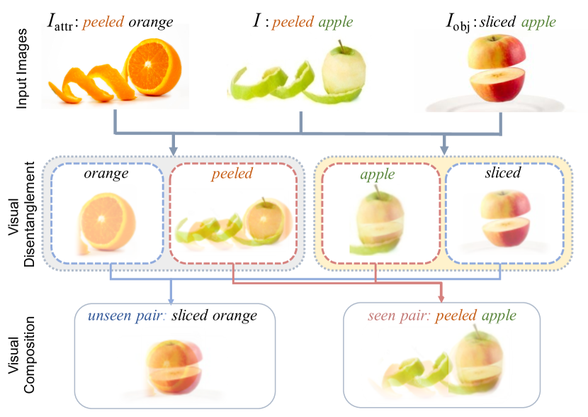
Figure 1: Method illustration: Given an input image $I$ of peeled apple, we use two other images: (1) one with same object, different attribute ${I_{\text{obj}}}$ - sliced apple, (2) one with same attribute, different object ${I_{\text{attr}}}$ - peeled orange. We propose a novel architecture that takes $I$ and ${I_{\text{attr}}}$, and extracts their visual similarity features for peeled and visual dissimilarity features for orange. Similarly, using $I$ and ${I_{\text{obj}}}$, the visual similarity features for apple, and the dissimilarity features for sliced can be extracted. We compose these primitive visual features to hallucinate a seen pair peeled apple, and a novel unseen pair sliced orange to be used for regularizing our embedding space. Note that this is a visualization of embedding space composition, we do not generate images.

This idea dates back to Recognition and Composition theory by Biederman [8], and early work in the visual domain by Hoffman [25], which proposed recognition by parts for pose estimation. Prior works explore compositionality to a certain degree, e.g., via feature sharing and shared embeddings space. Among them, most works use linguistically inspired losses to separate attributes and objects in the shared embedding space, then use that primitive knowledge to compose new complex pairs. Using linguistic embeddings is helpful since: (1) there is a clear distinction between attribute and object in the embedding space, and (2) these embeddings already contain semantic knowledge of similar objects and attributes, which is helpful for composition. However, unlike word embedding, it is difficult to discriminate the object and attribute in the visual embedding space.

This is due to the fact that image feature extractor is usually pre-trained for object classification, often along with image augmentation (e.g., color jitter) that tends to produce attribute-invariant image representation, thus does not learn objects and attributes separately. In this paper, we propose a new direction that focuses on visual cues, instead of using linguistic cues explicitly for novel compositions.

Analogous to linguistic embedding, our work focuses on disentangling attribute and object in the visual space. Our method, Object Attribute Disentanglement (OADis), learns distinct and independent visual embeddings for peeled and apple from the visual feature of peeled apple. As shown in Figure 1, for image $I$ of peeled apple, we use two other images: one with same object and different attribute ${I_{\text{obj}}}$ (e.g., sliced apple), and one with same attribute and different object ${I_{\text{attr}}}$ (e.g., peeled orange). OADis takes $I$ and ${I_{\text{obj}}}$ and learns the similarity (apple) and dissimilarity (sliced) of the second image with respect to the first one. Similarly, using $I$ and ${I_{\text{attr}}}$, the commonality between them (peeled) and the left out dissimilarity (orange) can also be extracted. Further, composition of these extracted visual primitives are used to hallucinate seen and unseen pair, peeled apple and sliced orange respectively.

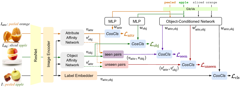
Figure 2: System Overview: Given an image $I$, for peeled apple, we consider two images:, one with same object: ${I_{\text{obj}}}$, sliced apple, and one with same attribute, ${I_{\text{attr}}}$ peeled orange. (1) The Object-Conditioned Network composes pair word embedding, using GloVe word embeddings for labels. (2) Label Embedder uses the image $I$ and embeds visual feature ${v_{\text{attr,obj}}}$ along with word embedding ${w_{\text{attr,obj}}}$, using loss ${\mathcal{L}_{\text{cls}}}$. (3) Attribute Affinity Network and Object Affinity Network, disentangles the same attribute and object from the pair of images $I,{I_{\text{attr}}}$ and $I,{I_{\text{obj}}}$ respectively. Disentangled visual features for peeled (${v_{\text{attr}}}$) and apple (${v_{\text{obj}}}$) are used along with word embeddings of attribute (${w_{\text{attr}}}$) and objects (${w_{\text{obj}}}$), to compute ${\mathcal{L}_{\text{attr}}}$ and ${\mathcal{L}_{\text{obj}}}$. (4) Using disentangled features, we compose seen pair peeled apple (${v_{\text{attr}}},{v_{\text{obj}}}$) and unseen pair sliced orange (${v_{\text{attr}}^{\prime}},{v_{\text{obj}}^{\prime}}$), for composition losses ${\mathcal{L}_{\text{seen}}}$ and ${\mathcal{L}_{\text{unseen}}}$.

For compositional learning, it is necessary to decompose first before composing new unseen attribute-object pairs. As humans, we have the ability to imagine an unseen complex concept using previous knowledge of its primitive concepts. For example, if someone has seen a clown and a unicycle, they can imagine clown on a unicycle even if they have never seen this combination in real life [47, 23]. This quality of imagination is the basis of various works such as GANs [15], CLIP [51] and DALL-E [52]. However, these works rely on larger datasets and high computation power for training. We study this idea of imagination for a smaller setup by composing newer complex concepts using disentangled attributes and object visual features. Our work focuses on answering the question, can there be visual embedding of peeled and apple, disentangled separately from visual feature of peeled apple? Our contributions are as follows:

• We propose a novel approach, OADis, to disentangle attribute and object visual features, where visual embedding for peeled is distinct and independent of embedding for apple.

• We compose unseen pairs in the visual space using the disentangled features. Following Compositional Zero-shot Learning (CZSL) setup, we show competitive improvement over prior works on standard datasets [27, 60].

• We propose a new large-scale benchmark for CZSL using an existing attribute dataset VAW [49], and show that OADis outperforms existing baselines.

2 Related Work

Visual Attributes. Visual attributes have been studied widely to understand visual properties and low-level semantics of objects. These attributes help further improve on various downstream tasks such as object detection [17, 29, 18, 7, 40, 14], action recognition [37, 21, 6, 5, 3, 19], image captioning [28, 44], and zero-shot and semi-supervised classification [45, 4, 30, 43, 13, 54, 14]. Similar to multi-class classification for objects, initial work for attribute understanding used discriminative models [29, 46], without understanding attributes. Other works [18, 35, 11, 26] explored the relation between the same attributes and different objects, to learn visual attributes. Particularly, disentangling object features from attribute features are explored in [20, 22]. Although, these works use clustering and probabilistic models to learn the attributes of objects.

Compositional Zero-shot Learning. Concept of compositional learning was first introduced in Recognition by Parts [25]. Initially, [39] employed this concept for objects and attributes. Unlike zero-shot learning (ZSL), CZSL requires the model to learn to compose unseen concepts from already learned primitive components. [39, 11] proposed separate classifiers for primitive components, and merged all into a final classifier. Most prior works use linguistically inspired auxiliary loss terms to regularize training for embedding space, such as: [42] models attributes as a linear transformation of objects,  [33] uses rules of symmetry for understanding states, and  [59] learns composition and decomposition of attributes hierarchically. Another set of studies uses language priors to learn unseen attribute-object pairs, either in feature space or with multiple networks [34, 50, 56]. Other recent works use graph structure to leverage information transfer between seen to unseen pairs using Graph Convolutional Networks [41, 36], and [58] uses key-query based attention, along with modular network with message passing for learning relation between primitive concepts.

3 Object Attribute Disentanglement (OADis)

Contrary to prior works [42, 33, 41, 59], we explicitly focus on separating attributes and object features in the visual space. More precisely, TMN [50] uses word embeddings to generate attention layers to probe image features corresponding to a given pair, GraphEmbedding [41] exploits the dependency between word embeddings of the labels, and HiDC [59] mainly uses word embeddings to compose novel pairs and generate more examples for their triplet loss. To the best of our knowledge, none of the existing works have explored visual feature disentanglement of attributes and objects. We hypothesize that attribute and object visual features can be separated when considering visual feature similarities and differences between image pairs. Composing these disentangled elements help regularize the common embedding space to improve recognition performance. More concretely, we take cues from [20] and [39, 59], to learn to compose unseen attribute-object pairs leveraging visual attributes based on auxiliary losses.

3.1 Task Formulation

We follow the conventional Compositional Zero-shot Learning (CZSL) setup, where distinct attribute-object compositions are used at training and testing. Each image $I$ is labeled with $y=y_{\text{attr,obj}}\in Y$, where $y_{\text{attr}}$ and $y_{\text{obj}}$ are respectively the attribute and object label. The dataset is divided into two parts, seen pairs $y^{s}\in Y^{s}$ and unseen pairs $y^{u}\in Y^{u}$, such that $Y=Y^{s}\cup Y^{u},Y^{s}\cap Y^{u}=\emptyset$. Although $y^{u}=y_{\text{attr,obj}}\in Y^{u}$ consists of attribute $y_{\text{attr}}$ and object $y_{\text{obj}}$ that are never seen together in training, they are separately seen. We employ the Generalized CZSL setup defined in [50], which has seen $Y^{s}$ and unseen pairs $Y^{u}$ in the validation and test sets as detailed in Table 1. As shown in Figure 2, for image $I$, with label peeled apple, we choose two additional images: one with same object and different attribute ${I_{\text{obj}}}$ (e.g., sliced apple), and another image with same attribute and different object ${I_{\text{attr}}}$ (e.g., peeled orange). Note that the subscript of image symbol, e.g., attr in ${I_{\text{attr}}}$, shows similarity with $I$, whereas superscript denotes seen and unseen sets.

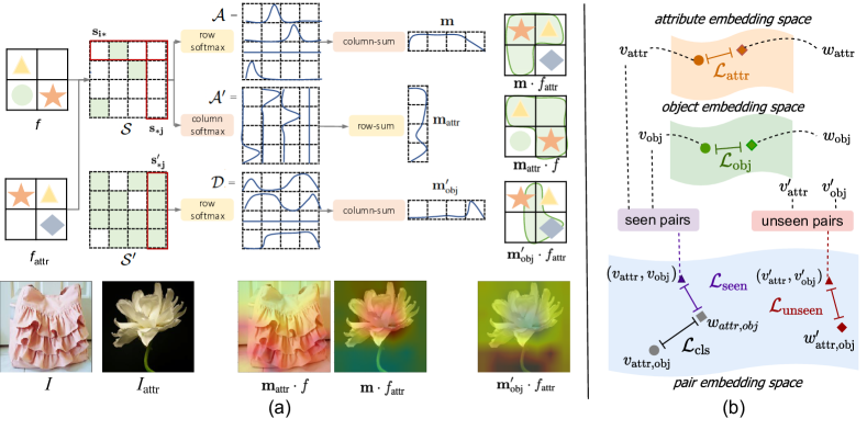
Figure 3: (a) Attribute Affinity Module: We compute the cosine similarity between blocks in $f$ and ${f_{\text{attr}}}$ ($S$ in Eq. 3), then apply row-wise and column-wise softmax (${\mathcal{A}}$ and ${\mathcal{A}^{\prime}}$), followed by a respective column-sum and row-sum to obtain $\mathbf{m}$ and $\mathbf{{m_{\text{attr}}}}$. $\mathbf{m}$ represents regions where ${f_{\text{attr}}}$ is highly similar to $f$ (hence, we reshape and multiply $\mathbf{m}$ with ${f_{\text{attr}}}$) and $\mathbf{{m_{\text{attr}}}}$ represents regions where $f$ is highly similar to ${f_{\text{attr}}}$ (thus, $\mathbf{{m_{\text{attr}}}}\cdot f$). Similarly, $S^{\prime}$ represents the regions where feature ${f_{\text{attr}}}$ is not similar to feature $f$ (more details in Section 3.2). The last row shows real samples and generated attention maps overlayed on images. Give image ruffled bag and ruffled flower, we show that attribute ruffle is highlighted in the center $\mathbf{{m_{\text{attr}}}}\cdot f$ and $\mathbf{m}\cdot{f_{\text{attr}}}$. Whereas, $\mathbf{{m_{\text{obj}}^{\prime}}}\cdot{f_{\text{attr}}}$ shows the dissimilar regions of ${I_{\text{attr}}}$ w.r.t $I$. (b) Shows the three embedding spaces learnt with different losses. Same notation is used as Figure 2.

3.2 Disentangling Visual Features

We extract image and label embedding features from pre-trained networks (ResNet [24] and GloVe [48]). As seen in Figure 2, we use Image Encoder (IE) and Object Conditioned Network (OCN), for image and word embedding features respectively. Similar to [42], we use Label Embedder (LE) as an additional FC-Layer for the image feature. LE and OCN learn image and word embeddings and embed those in a common pair embedding space. Next, visual similarity between $I$ and ${I_{\text{obj}}}$ is computed using Object Affinity Network, which extracts visual features for object, ${v_{\text{obj}}}$. Whatever is not similar is considered dissimilar. Hence, visual features of ${I_{\text{obj}}}$ that are least similar to visual features of $I$ are considered as the attribute feature ${v_{\text{attr}}^{\prime}}$ in ${I_{\text{obj}}}$, which is sliced in this example. Similarly, Attribute Affinity Network takes $I$ and ${I_{\text{attr}}}$, and extracts visual similarity feature ${v_{\text{attr}}}$ for peeled, and dissimilar visual features of ${I_{\text{attr}}}$, as object feature ${v_{\text{obj}}^{\prime}}$ for orange. The disentangled features are then used to compose seen and unseen pairs. We discuss the details in the following sections:

Image Encoder (IE). We use the second last layer before AveragePool of an ImageNet-pretrained ResNet-18 [24, 16] to extract features for all images. IE is a single convolutional layer that is shared across images $I$, ${I_{\text{attr}}}$ and ${I_{\text{obj}}}$ to generate their image features, represented as $f$, ${f_{\text{attr}}}$ and ${f_{\text{obj}}}$ respectively, where each $f\in\mathbb{R}^{n\times 49}$ and $n$ is the output dimension of IE.

Label Embedder (LE). Inspired by [42], our LE inputs spatial feature from ResNet [24], AveragePools and passes through a linear layer to extract final feature ${v_{\text{attr,obj}}}$ for pair embedding, which has same dimension as the word embedding final feature ${w_{\text{attr,obj}}}$, extracted from Object Conditioned Network (OCN) (Figure 2). This is the main branch, and is used for input image $I$ only.

Object Conditioned Network (OCN). This takes word embeddings of attribute $emb_{\text{attr}}$ and object $emb_{\text{obj}}$, concatenates the features and passes through multiple layers. Object-conditioned is named because a residual connection for the object feature is concatenated with the final attribute feature, and the output feature is ${w_{\text{attr,obj}}}\in Y$. We discuss the motivation for this in Section 4.3.

Cosine Classifier (CosCls). Analogous to compatibility function used in [41, 36], we use cross-entropy along with cosine similarity to get the final score for each pair. For visual features ${v_{\text{attr,obj}}}$ (from LE), and composed word embeddings ${w_{\text{attr,obj}}}$ (from OCN), CosCls provides logits for an image $I$. For instance, let us assume $v:X\rightarrow Z$ and $w:Y\rightarrow Z$. $Z$ is the common embedding space for word embeddings $w$ and visual embeddings $v$. Then classifier unit CosCls gives the score for label $y\in Y^{s}$ is $C$:

$$h(v,w)=\cos(v,w)=\delta\cdot\frac{v^{T}w}{\left\|v\right\|\left\|w\right\|}$$ (1)

$$C(v,w)=\frac{e^{h(v,w)}}{\sum_{y\in Y^{s}}e^{h(v,y)}}$$ (2)

where $\delta$ is the temperature variable. Each loss function uses same CosCls score evaluator, with different inputs.

Object and Attribute Similarity Modules. Our main contribution is the proposed affinity modules and compositional losses. Inspired by image captioning [31, 32, 12], OADis uses image similarities and differences to identify visual features corresponding to attributes and objects. Object Affinity Network (OAN) uses $f$ and ${f_{\text{obj}}}$, whereas Attribute Affinity Network (AAN) uses $f$ and ${f_{\text{attr}}}$. For brevity, we explain the AAN, while the OAN follows the same architecture. Reminded that both $f$ and ${f_{\text{attr}}}\in\mathbb{R}^{n\times 49}$.

Similar to [57], which computes attention between word concepts with corresponding visual blocks, we compute attention between two images $I$ and ${I_{\text{attr}}}$. Since both images have the same attribute, i.e., peeled, our affinity network learns visual similarity between the images, which represents the attribute. Similarity matrix $\mathcal{S}$ is the cosine similarity between $f$ and ${f_{\text{attr}}}$, such that $\mathcal{S}\in\mathbb{R}^{49\times 49}$ as:

$$\mathcal{S}=\frac{f^{T}{f_{\text{attr}}}}{\left\|f\right\|_{2}\left\|{{f_{\text{attr}}}}\right\|_{2}}\vspace{-.1in}$$ (3)

where element $s_{ij}$ represents the similarity between $i^{\text{th}}$ element of $f$ with $j^{\text{th}}$ element of ${f_{\text{attr}}}$. Moreover, let $\mathbf{s_{i*}}$ and $\mathbf{s_{*j}}$ represent the $i^{\text{th}}$ row and $j^{\text{th}}$ column of $\mathcal{S}$ respectively. Then, $\mathbf{s_{i*}}$ captures the similarity of all the elements in ${f_{\text{attr}}}$ with respect to $i^{\text{th}}$ element of $f$. To know the most similar element among ${f_{\text{attr}}}$ with respect to $i^{\text{th}}$ element of $f$, we can take a row-wise softmax over $\mathcal{S}$. Similarly, for $j^{\text{th}}$ element of ${f_{\text{attr}}}$, column $\mathbf{s_{*j}}$ represents the similarity with all the elements of $f$. Using a column-wise softmax, we can interpret the most similar and least similar element of $f$ with respect to $j^{\text{th}}$ element of ${f_{\text{attr}}}$, as shown in Figure 3. Therefore, by applying column-wise and row-wise softmax, we get two matrices, ${\mathcal{A}}$ and ${\mathcal{A}^{\prime}}$ (${\mathcal{A}},{\mathcal{A}^{\prime}}\in\mathbb{R}^{d\times d},d=49$),

$${\mathcal{A}}_{i}=\frac{e^{\lambda\mathbf{s_{i*}}}}{\sum_{j=1}^{d}e^{\lambda s_{ij}}}\quad\text{and}\quad{\mathcal{A}^{\prime}}_{j}=\frac{e^{\lambda\mathbf{s_{*j}}}}{\sum_{i=1}^{d}e^{\lambda s_{ij}}},$$ (4)

where $\lambda$ is the inverse temperature parameter. We compute row and column sum for ${\mathcal{A}}$ and ${\mathcal{A}^{\prime}}$ respectively, to get final similarity maps, $\mathbf{m}$ and $\mathbf{{m_{\text{attr}}}}$,

$$m_{j}=\sum_{i=1}^{d}{\mathcal{A}}_{ij}\quad\text{and}\quad{{m_{\text{attr}}}}_{i}=\sum_{j=1}^{d}{\mathcal{A}^{\prime}}_{ij}.$$ (5)

Similarly, the difference between these two images $f$ and ${f_{\text{attr}}}$ is the object label, ${y_{\text{obj}}}$. Hence, we use the negative of $\mathcal{S}$ as the image difference, denoted as ${\mathcal{S}^{\prime}}$. Then, difference of ${f_{\text{attr}}}$ with respect to $f$ would be row-wise softmax of difference matrix, denoted by ${\mathcal{D}}$. Hence, by performing column-sum over ${\mathcal{D}}$, we get difference map, $\mathbf{{m_{\text{obj}}^{\prime}}}$,

$$\mathcal{D}_{j}=\frac{e^{\gamma\mathbf{s^{\prime}_{*j}}}}{\sum_{i=1}^{d}e^{\gamma s^{\prime}_{ij}}}\quad\text{and}\quad{{m_{\text{obj}}^{\prime}}}_{i}=\sum_{j=1}^{d}{\mathcal{D}}_{ij}.$$ (6)

The final disentangled features for attribute ${v_{\text{attr}}}$ and object ${v_{\text{obj}}^{\prime}}$, for both AAN and OAN, can be computed as:

$$\begin{split}{v_{\text{attr}}}=\mathbf{m}\cdot{f_{\text{attr}}}+\mathbf{{m_{\text{attr}}}}\cdot f\quad&\text{and}\quad{v_{\text{obj}}^{\prime}}=\mathbf{{m_{\text{obj}}^{\prime}}}\cdot{f_{\text{attr}}}\\ {v_{\text{obj}}}=\mathbf{m}\cdot{f_{\text{obj}}}+\mathbf{{m_{\text{obj}}}}\cdot f\quad&\text{and}\quad{v_{\text{attr}}^{\prime}}=\mathbf{{m_{\text{attr}}^{\prime}}}\cdot{f_{\text{obj}}}.\end{split}$$ (7)

More details using a toy example can be seen in Figure 3. Using concatenation of ${v_{\text{attr}}}$ and ${v_{\text{obj}}}$ along with a single Linear layer, composes the pair peeled apple, represented by $({v_{\text{attr}}},{v_{\text{obj}}})$. Similarly, the disentangled visual features ${v_{\text{attr}}^{\prime}}$ and ${v_{\text{obj}}^{\prime}}$, are used to compose unseen pair sliced orange, and is represented as $({v_{\text{attr}}^{\prime}},{v_{\text{obj}}^{\prime}})$.

3.3 Embedding Space Learning objectives

As shown in Figure 3b, we learn three embedding spaces: (1) attributes space, (2) object space, and (3) attribute-object pair space. The attribute and object spaces are used for disentangling the two, whereas pair embedding is used for final pair composition and inference. OADis has separate loss functions for disentangling and composing. All loss functions are expressed in terms of CosCls defined previously.

The loss function for main branch, ${\mathcal{L}_{\text{cls}}}$ uses combined visual feature ${v_{\text{attr,obj}}}$ from LE and word embedding feature ${w_{\text{attr,obj}}}$ from OCN. ${\mathcal{L}_{\text{cls}}}$ is used for the pair embedding space. Similarly, ${\mathcal{L}_{\text{attr}}}$ and ${\mathcal{L}_{\text{obj}}}$ are used to learn the visual attribute and object feature, in their respective embedding spaces. ${\mathcal{L}_{\text{attr}}}$ pushes the visual feature of attribute, closer to the word embedding. ${\mathcal{L}_{\text{obj}}}$ does the same for objects in object embedding space Figure 3b. These losses cover the concept of disentanglement, and can be represented as:

$$\begin{split}{\mathcal{L}_{\text{cls}}}&=C({v_{\text{attr,obj}}},{w_{\text{attr,obj}}})\\ {\mathcal{L}_{\text{attr}}}&=C({v_{\text{attr}}},{w_{\text{attr}}});\,\,{\mathcal{L}_{\text{obj}}}=C({v_{\text{obj}}},{w_{\text{obj}}})\\ \end{split}$$ (8)

For composition, we use ${\mathcal{L}_{\text{seen}}}$ and ${\mathcal{L}_{\text{unseen}}}$. Among the images seen ($I$, ${I_{\text{attr}}}$, and ${I_{\text{obj}}}$), disentangled features ${v_{\text{obj}}}$ and ${v_{\text{attr}}}$, composes the same pair as $({v_{\text{attr}}},{v_{\text{obj}}})$, which we refer to as the seen composition. Note that $({v_{\text{attr}}},{v_{\text{obj}}})$ is different from ${v_{\text{attr,obj}}}$, as the former is hallucinated feature with combination of disentangled attribute and object visual features, and latter is the combined visual feature extracted with LE. Here, we use ${\mathcal{L}_{\text{seen}}}$ loss which takes the composition of disentangled features and learns to put the composition closer to ${w_{\text{attr,obj}}}$. Moreover, the dissimilarity aspect from OAN and AAN extracts ${v_{\text{attr}}^{\prime}}$ and ${v_{\text{obj}}^{\prime}}$, which composes an unseen pair $({v_{\text{attr}}^{\prime}},{v_{\text{obj}}^{\prime}})$. We use ${\mathcal{L}_{\text{unseen}}}$ as unseen loss since the hallucinated composition is never seen among $I$ , ${I_{\text{attr}}}$, and ${I_{\text{obj}}}$.

$$\begin{split}{\mathcal{L}_{\text{seen}}}&=C(({v_{\text{attr}}},{v_{\text{obj}}}),{w_{\text{attr,obj}}})\\ {\mathcal{L}_{\text{unseen}}}&=C(({v_{\text{attr}}^{\prime}},{v_{\text{obj}}^{\prime}}),{w_{\text{attr,obj}}^{\prime}})\\ \end{split}$$ (9)

The combined loss function $\mathcal{L}$ is minimized over all the training images, to train OADis end-to-end. The weights for each loss ($\mathcal{\alpha}$) are empirically computed:

$$\begin{split}\mathcal{L}&={\mathcal{L}_{\text{cls}}}+\alpha_{1}{\mathcal{L}_{\text{attr}}}+\alpha_{2}{\mathcal{L}_{\text{obj}}}+\alpha_{3}{\mathcal{L}_{\text{seen}}}+\alpha_{4}{\mathcal{L}_{\text{unseen}}}.\end{split}$$

Table 1: This table shows dataset splits. $Y^{s}$ and $Y^{u}$ are seen and unseen compositions respectively. We propose a new benchmarck, VAW-CZSL [49], which has more than 10$\times$ compositions in each split compared to other datasets.

	Train set			Val set	Test set
Datasets	attr.	obj.	$Y^{s}$	$Y^{s}/Y^{u}$	$Y^{s}/Y^{u}$
MIT-states [27]	115	245	1262	300 / 300	400 / 400
UT-Zappos [60]	16	12	83	15 / 15	18 / 18
VAW-CZSL [49]	440	541	11175	2121 / 2322	2449 / 2470

Table 2: We show results on MIT-states [27] and UT-Zappos [60]. Following [41, 50], we use AUC in % between seen and unseen compositions with different bias terms, along with Val, Test, attribute and object accuracy. HM is Harmonic Mean. OADis consistently outperforms on most categories with significant increment.

	MIT-States							UT-Zappos
Model	Val@1	Test@1	HM	Seen	Unseen	Attribute	Object		Val@1	Test@1	HM	Seen	Unseen	Attribute	Object
AttrOpr [42]	2.5	2.0	10.7	16.6	18.4	22.9	24.7		29.9	22.8	38.1	55.5	54.4	38.6	70.0
LabelEmbed+ [42]	3.5	2.3	11.5	16.2	21.2	25.6	27.5		35.5	22.6	37.7	53.3	58.6	40.9	69.1
TMN [50]	3.3	2.6	11.8	22.7	17.1	21.3	24.2		35.9	28.4	44.0	58.2	58.0	40.8	68.4
Symnet [33]	4.5	3.4	13.8	24.8	20.0	26.1	25.7		27.4	27.7	42.5	56.7	61.6	44.0	70.6
CompCos [36]	6.9	4.8	16.9	26.9	24.5	28.3	31.9		40.8	26.9	41.1	57.7	62.8	43.3	73.0
GraphEmb [41]	7.2	5.3	18.1	28.9	25.0	27.2	32.5		33.9	24.7	38.9	58.8	61.0	44.0	72.6
OADis	7.6	5.9	18.9	31.1	25.6	28.4	33.2		40.8	30.0	44.4	59.5	65.5	46.5	75.5

4 Experiment

Table 3: We show results on VAW-CZSL. Since it is a much more challenging dataset, with significantly large number of compositions, to discriminate performance among different baseline, we show top-3 and top-5 AUC (in %) for Val and Test sets.

	Val. Set		Test Set
Model	V@3	V@5	V@3	V@5	HM	Seen	Unseen	Attr.	Obj.
AttrOpr [42]	1.4	2.5	1.4	2.6	9.1	16.4	11.7	13.7	34.9
LabelEmbed+ [42]	1.5	2.8	1.6	2.8	9.8	16.2	13.2	13.4	35.1
Symnet [33]	2.3	3.9	2.3	3.9	12.2	19.1	15.8	18.6	40.9
TMN [50]	2.2	3.9	2.3	4.0	11.9	19.9	15.4	15.9	38.3
CompCos [36]	3.1	5.6	3.2	5.6	14.2	23.9	18.0	16.9	41.9
GraphEmb [41]	2.7	5.3	2.9	5.1	13.0	23.4	16.8	16.9	40.8
OADis	3.5	6.0	3.6	6.1	15.2	24.9	18.7	17.5	43.3

4.1 Datasets and Metrics

We show results on three datasets: MIT-states [27], UT-Zappos [60], and a new benchmark for evaluating CZSL on images of objects in-the-wild, referred as VAW-CZSL. VAW-CZSL is created based on images with object and attribute labels from the VAW dataset [49]. Both MIT-states [27] and UT-Zappos [60] are common datasets used for this task in previous studies. MIT-states covers wide range of objects (i.e., laptop, fruits, fish, room, etc.) and attributes (i.e., mossy, dirty, raw, etc.), whereas UT-zappos has fewer objects (i.e., shoes type: boots, slippers, sandals) and fine-grained attributes (i.e., leather, fur, etc.).

Proposed New Benchmark. While experimenting with MIT-states [27] and UT-Zappos [60], we found several shortcomings with these datasets and discovered issues across all baselines using these datasets:

• Both datasets are small, with a maximum of 2000 attribute-object pairs and 30k images, leading to overfitting fairly quickly.

• Random seed initialization makes performance fluctuate significantly (0.2-0.4% AUC). Moreover, [4] found 70% noise in human-annotated labels on MIT-States [27].

• A new dataset C-GQA was introduced in [41], but the dataset is still small and we found a lot of discrepancies (kindly refer to the suppl.).

To address these limitations, we propose a new benchmark VAW-CZSL, a subset of VAW [49], which is a multi-label attribute-object dataset. We sample one attribute per image, leading to much larger dataset in comparison to previous datasets as shown in Table 1 (details in the suppl.).

Evaluation. We use Generalized CZSL setup, defined in [50], with dataset statistics presented in Table 1. As observed in prior works [41, 50], a model trained on a set of labels $Y^{s}$, does not generalize well on unseen pairs $Y^{u}$. Therefore, [41, 50] use a scalar term for overcoming the negative bias for unseen pairs. We use the same evaluation protocol, which computes Area Under the Curve (AUC) (in %) between the accuracy on seen and unseen compositions with different bias terms [50]. Larger bias term leads to better results for unseen pairs whereas smaller bias leads to better results for seen pairs. Harmonic mean is reported, to balance the bias. We also report the attribute and object accuracy for unseen pairs, to show improvement due to visual disentanglement of features. Our new benchmark subset for VAW [49], follows the similar split as other datasets. In addition, we conduct all experiments with image augmentation for all methods (discussed in Section 4.3).

4.2 Results and Discussion

Baselines. We compare with related recent and prominent prior works: AttrOp [42], LabelEmbed+ [42], TMN [50], Symnet [33], CompCos [36] and GraphEmb [41]. We do not compare with BMP [58], since it uses the concatenation of features from all four ResNet blocks (960-d features), resulting in higher input features and the number of network parameters than all other setups. Moreover, GraphEmb [41] is state-of-the-art; hence, comparing with that makes our work comparable to other baselines that [41] already outperforms. To be consistent, we state the performance of all models (including GraphEmb [41]) using frozen backbone ResNet without fine-tuning the image features, and using GloVe [48] for the object and attribute word embeddings. Before passing through backbone, training images are augmented with horizontal flip and random crop. Compared to other baselines, OADis uses convolutional features rather than AvgPooled, since it is easier to segregate visual features in the spatial domain for attributes and objects. Moreover, other studies [41, 36] have also used additional FC layers on top of IE, which we argue makes it fair for us to use pre-pooled features for OADis.

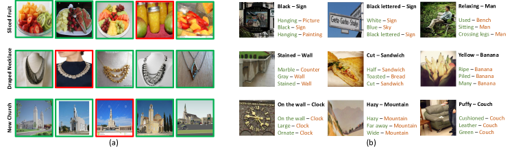
Figure 4: Qualitative Results: We show the nearest neighbors using the hallucinated unseen composition features for MIT-states and UT-Zappos. Although, all the neighbors are not correct (represented with red outline), they look very similar to true class labels: (a) First row: pureed fruit, Second row: engraved coin, Third row: huge tower. (b) We show top-3 predictions for images in VAW-CZSL.

Table 4: We quantitatively show that the proposed architecture and different losses help in disentanglement and composition of unseen pairs. The experiments are conducted on MIT-States [27], where change in accuracy is shown with green and red based on increment or decrement respectively from the previous row. A dash (-) represents no change more than ($\pm$ 0.1). Refer to Section 4.2 for details.

Losses	Val AUC@1	Test AUC@1	Seen	Unseen	Attribute	Object
${\mathcal{L}_{\text{cls}}}$	7.24	5.43	29.92	25.33	28.03	33.10
${\mathcal{L}_{\text{cls}}}$ + ${\mathcal{L}_{\text{attr}}}$	-	-	31.09 (+2.0)	-	28.30 (+0.3)	-
${\mathcal{L}_{\text{cls}}}$ + ${\mathcal{L}_{\text{obj}}}$	-	-	-	25.50 (+0.2)	-	33.38 (+0.2)
${\mathcal{L}_{\text{cls}}}$ + ${\mathcal{L}_{\text{attr}}}$ + ${\mathcal{L}_{\text{obj}}}$	7.49 (+0.2)	5.73 (+0.2)	-	-	28.50 (+0.2)	-
${\mathcal{L}_{\text{cls}}}$ + ${\mathcal{L}_{\text{attr}}}$ + ${\mathcal{L}_{\text{obj}}}$ + ${\mathcal{L}_{\text{seen}}}$	-	5.44 (-0.5)	31.21 (+0.2)	-	28.18 (-0.4)	-
${\mathcal{L}_{\text{cls}}}$ + ${\mathcal{L}_{\text{attr}}}$ + ${\mathcal{L}_{\text{obj}}}$ + ${\mathcal{L}_{\text{unseen}}}$	-	5.73 (+0.3)	-	25.80 (+0.4)	28.51 (+0.4)	-
${\mathcal{L}_{\text{cls}}}$ + ${\mathcal{L}_{\text{attr}}}$ + ${\mathcal{L}_{\text{obj}}}$ + ${\mathcal{L}_{\text{seen}}}$ + ${\mathcal{L}_{\text{unseen}}}$	7.62 (+0.2)	5.94 (+0.2)	31.64 (+0.4)	25.60 (-0.2)	28.51	33.20

Table 5: Results with different networks for word-embeddings. Object-conditioning with attribute performs the best, and is therefore used for OADis (Section 4.3).

	Linear	MLP	Obj-cond. Network
Val@1	6.6	7.0	7.6
Test@1	5.0	5.2	5.9

Results on MIT-States. MIT-states has considerable label noise [4], but still is a standard dataset for this task. We show significant improvement on this dataset (reported in Table 2), from previous state-of-the-art GraphEmb, which has 7.2 Val AUC and 5.3 Test AUC. Note that we do not report GraphEmb results with fine-tuning backbone, as we find it incomparable with other baselines that did not incorporate fine-tuning as part of their proposed methods. Overall, our model performs significantly better than GraphEmb on all metrics.

Results on UT-Zappos. Similar improvement trends hold for UT-Zapopos as well (see Table 2). Although, as explained for GraphEmb, it is difficult to balance the best performance for Val and Test set in this dataset. The problem is that 7/36 ($\sim$20%) attributes in Test set do not appear in Val set. Hence, improving Val set AUC, does not necessarily improve Test AUC for UT-Zappos. Similar trend can be seen for other baselines: CompCos has best Val AUC, but does not perform well on Test set, compared to TMN and Symnet. Even GraphEmb in their final table show the frozen backbone network has much lower performance than TMN. However, OADis performs well on UT-Zappos overall, with $\sim$4.0 improvement for Val and Test AUC, HM, unseen and object accuracy.

Results on VAW-CZSL. Our model performs well on VAW-CZSL, and is consistently better than other methods across almost all metrics. As shown in Table 1, VAW-CZSL has $\sim$6-8 times more pairs in each split than MIT-States, which shows how challenging the benchmark is. Due to top-1 AUC being too small to quantify any learning and comparing between methods, we report top-3 and top-5 AUC instead. This is also because objects in-the-wild tend to depict multiple possible attributes; hence, evaluating only the top-1 prediction is insufficient. We provide qualitative results of how our model makes object-attribute composition prediction on VAW-CZSL in the suppl.

Is disentangling and hallucinating pairs helpful? Prior works rely heavily on word embeddings for this task, but to improve the capabilities of visual systems, it is imperative to explore what is possible in the visual domain. We do an extensive study to understand if our intuition aligns with OADis (Table 4). Here are some takeaways:

• Using only ${\mathcal{L}_{\text{cls}}}$, we get a benchmark performance based on the architectural contributions, such as LE and ONC. When ${\mathcal{L}_{\text{attr}}}$ is added, significant performance boost for attribute accuracy can be seen in Table 4.

• Adding object loss ${\mathcal{L}_{\text{obj}}}$ with ${\mathcal{L}_{\text{cls}}}$, makes object accuracy better but no change in Val and Test AUC. This indicates the need of both losses to balance the effects. Using both ${\mathcal{L}_{\text{attr}}}$ and ${\mathcal{L}_{\text{obj}}}$ gives improvement in all measures.

• Adding ${\mathcal{L}_{\text{seen}}}$ results in boost for seen AUC, but drop in Test AUC, which has unseen pairs along with seen pairs. Using unseen loss ${\mathcal{L}_{\text{unseen}}}$ leads to increase in both Test and attribute accuracy.

• Finally adding unseen composition loss ${\mathcal{L}_{\text{unseen}}}$ along with seen loss ${\mathcal{L}_{\text{seen}}}$, the model improves on most metrics. Each loss plays a role and regularizes effects from other losses.

Is visual disentangling actually happening? Visual disentanglement in feature space is challenging to visualize since: (a) parts of an image for attributes and objects are hard to distinguish, as attributes are aspects of an object; (b) OADis is end-to-end trained with losses to disentangle features for attribute and object embeddings, which is separate from pair embedding space. Inspired by [42, 33], we show a few qualitative results in Figure 5. Using all training images, prototype features $\mathcal{V_{\text{attr}}}$ for each attribute can be computed by averaging features for all images containing that attributes ${v_{\text{attr}}}$ using AAN. Similarly, with OAN, prototype object features are also computed. For each test image, we find top-3 nearest neighbors from these prototype features (Figure 5). Hence, the disentangled prototype features of attributes and objects are used for classifying unseen images. Note that results reported in Table 1 use pair embedding space for attribute and object classification, whereas here we use auxiliary attribute and object embedding spaces (in Figure 3b) for the same task. If disentanglement features are not robust, then composition features will also not be efficient. We also show that using the composition of disentangled features for unseen pairs, relevant images from the test set can be found in suppl.

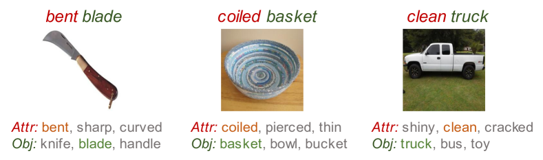
Figure 5: Qualitative results showing top 3 attributes and objects from test images, using prototype disentangled features computed on training data.

Limitations. Despite OADis outperforming prior works on all benchmarks, we still notice some outstanding deficiencies in this problem domain. First, similar to [41], OADis often struggles on images containing multiple objects, where it does not know which object to make prediction on. One possible solution is to utilize an object-conditioned attention that allows the model to focus and possibly output attribute for multiple objects. Second, from qualitative studies on VAW-CZSL, we notice there are multiple cases where OADis makes the correct prediction but is considered incorrect by the image label. This is due to the fact that objects in-the-wild are mostly multi-label (containing multiple attributes), which none of the current single-label benchmarks have attempted to address.

4.3 Ablation Studies

In this section, we show experiments to support our design choices for OADis. All the ablations are done for MIT-states [27], for one random seed initialization, and are consistent for other datasets as well. Empirical results for $\lambda$, $\delta$ and different word embeddings can be found in suppl.

Why Object-Conditioned Network? Label Embedder [42] uses a linear layer and concatenates word embeddings for attributes and objects. We experiment with other networks: MLP with more parameters with two layers and ReLU and Object-conditioned network that uses a residual connection for object embedding. Our intuition is that same attribute contributes differently to each object, i.e., ruffled bag is very different from ruffled flower. Hence, attributes are conditioned on object. Adding a residual connection for object embeddings to the final attribute embedding helps condition the attribute. We empirically demonstrate that object-conditioning helps in Table 5 (refer to the suppl.).

To augment or not to augment? Augmentation is a common technique to reduce over-fitting and improve generalization. Surprisingly, prior works do not use any image augmentation. OADis without augmentation gives 6.7% AUC on Val and 5.1% AUC on Test set for MIT-states. Hence, we use augmentation for OADis and re-implemented rest of the baselines in Table 2, showing that augmentation helps improving all methods $\sim$1.0-1.5% AUC. We use horizontal flip and random crop as augmentation.

4.4 Qualitative results

To qualitatively analyze our hallucinated compositions, we perform a nearest neighbor search on all three datasets. We pick the unseen compositions composed using the disentangled features, and find their top-5 nearest neighbors from the validation and test set. Figure 4(a) illustrates a few of our results. Note that these pairs are never seen in training. Based on the hallucinated compositions of disentangled attributes and objects, we are able to retrieve samples from these unseen compositions.

In Figure 4(b), we show the top-3 predictions of OADis on VAW-CSZL. Column 1 shows results for seen, and columns 2 and 3 show unseen compositions, with the ground-truth label on top (bold black). In all examples, our top-3 predictions describe the visual content of the images accurately, even though in many cases the ground-truth label is not predicted in top-1. For column 3, we purposely show examples where our model predictions totally differ from the ground-truth label, but still correctly describe the visual information in each image. Similar to [41], this explains the multi-label nature of object-attribute recognition, and why we report top-3 and top-5 metrics for the VAW-CZSL benchmark.

5 Conclusion

In this work, we demonstrated the ability to disentangle object and attribute in the visual feature space, that are used for hallucinating novel complex concepts, as well as regularizing and obtaining a better object-attribute recognition model. Through extensive experiments, we show the efficacy of our method, and surpass previous methods across three different benchmarks. In addition, we also propose a new benchmark for the compositional zero-shot learning task with images of objects in-the-wild, which we believe can help shift the focus of the community towards images in more complex scenes. Finally, we also highlight limitations of our work, including the notable problem of multi-label in object attributes, which we hope would encourage future works to start tackling CSZL for more realistic scenarios.

Acknowledgements. This work was supported by the Air Force (STTR awards FA865019P6014, FA864920C0010), DARPA SAILON program (W911NF2020009) and gifts from Adobe collaboration support fund.

Appendix

Appendix A Dataset issues of C-GQA [41]

GraphEmb [41] proposes a new benchmark for compositional zero-shot learning. However, there are some issues with the dataset have been raised on their official github page [1, 2]. These issues are related to (1) the attribute-object pairs being placed into the incorrect train, validation, and test subset, and (2) there are missing images for a decent amount of pairs (20%), which could potentially affect the final experiment results. Due to [41] being unable to provide a corrected version of the dataset in time before the CVPR 2022 deadline, we were unable to run any experiments for C-GQA. Post the deadline, we did run some preliminary results where our method outperformed GraphEmb [41]. Although, a major issue we observed was for OADis, C-GQA [41] training set did not have similar attributes and objects samples for constructing ${I_{\text{attr}}}$ and ${I_{\text{obj}}}$. However, we propose for learning compositional concepts, firstly disentangled concepts must be learnt, and for that, we require ${I_{\text{attr}}}$ and ${I_{\text{obj}}}$. Hence, we do not report results on C-GQA for OADis.

Appendix B Dataset Creation: VAW-CZSL

We propose a new benchmark for the compositional zero-shot learning task (CZSL), focusing on images of objects and attributes in the wild that span across a much larger number of categories. We select the VAW dataset [49] to create our benchmark. VAW contains images originally from Visual Genome (thus objects and attributes in the wild). Every image of an object instance contains an object label and one (or possibly multiple) attribute labels. In the followings, we describe our steps in creating the VAW-CZSL benchmark, which shares some similarities with the C-GQA dataset.

Different from C-GQA, we consider object instances whose bounding boxes are larger than 50 x 50. C-GQA selected instances whose boxes are larger than 112 x 112, which could possibly leave out small, narrow objects that are still recognizable from images. For every object instance, among its possibly multiple attributes label, we keep only one attribute that has the lowest frequency in the dataset (i.e., the uncommon attribute) to be consistent with the standard CZSL benchmark. By keeping the most uncommon attribute and using the top-3 & 5 evaluation metrics, all methods will be evaluated based on whether they are able to rank this uncommon (but still representative) attribute in its top-3 & 5 predictions rather than always predicting the most frequent attributes. From this, we follow the similar steps from [41] to merge plurals and synonyms (e.g., {airplane, plane, aeroplane, airplanes…}, {rock, stone, rocks…}). We then keep only those attribute and object categories with frequency greater than 30 to make sure all primitive concepts have a decent amount of data for training and evaluating.

We use images in VAW-training as our training set, and use images in VAW-val and VAW-test for creating the validation and testing splits following the standard generalized benchmark in CZSL. We first merge VAW-val and VAW-test in one set, and follow similar steps mentioned in [41] to create a validation and test set of seen and unseen attribute-object pairs. At the end, we remove objects and attributes that no longer appear in the training set. This is because a model that has never seen an attribute (or object) will find it impossible to generalize to unseen pairs containing this attribute (or object). This problem happens with the C-GQA dataset where  8% of attribute and  22% of object categories do not exist in their training set. More details about dataset can be found in Table 6. The dataset splits are made publicly available at https://github.com/nirat1606/OADis.

Appendix C Implementation Details

Following baselines, we use ResNet18 [24] pre-trained on Imagenet [16] as backbone feature extractor. Since, proposed auxiliary losses leverage image features, we use a single convolutional layer with Batch Normalization, ReLU and dropout for Image embedder with output dimension 1024 and dropout as 0.3. Note that we extract ResNet features before average pool. For word embeddings, we initialize with GLoVe [48]. Object Conditioned network, uses multiple linear layers, first for objects and attributes separately, then for concatenated features. Label embedder takes 1024-$d$ feature, performs AveragePool and finally embeds in a 300-$d$ space. Each loss uses compatibility function, i.e. cosine similarity, followed by cross-entropy loss over the compatibility function. Object similarity and attribute similarity modules also use two linear layers with dropout 0.05. On UT-Zappos, because the dataset is very small, we find using a linear layer (a smaller and simpler module than OCN) with dropout 0.1 results in better performance. We use Adam optimizer with weight decay $5e^{-5}$, and learning rate $2.5e^{-6}$ for the GLoVe embedding. The learning rate for the rest of the model is $3e^{-4}$ on MIT-States, and $1e^{-4}$ on UT-Zappos and VAW-CZSL. We decay the learning rate by 10 at epoch 30 and 40 on MIT-States, at epoch 50 on UT-Zappos, and at epoch 70 on VAW-CZSL. OADis needs to be trained for 70-150 epochs depending on the dataset, and training time is comparable with other methods (5-7 hours). These implementation details are also provided in our released source code.

Table 6: Dataset Details: This table shows the statistics for different datasets and their splits. The proposed VAW-CZSL benchmark significantly increases the number of attributes and objects.

			Train set			Val set			Test set
Datasets:	Attr.	Obj.	Seen Pairs.	# Images	Seen Pairs	Unseen Pairs	# Images	Seen Pairs	Unseen Pairs	# Images
MIT-States [27]	115	245	1262	30338	300	300	10420	400	400	12995
UT-Zappos [60]	16	12	83	22998	15	15	3214	18	18	2914
VAW-CZSL [49]	440	541	11175	72203	2121	2322	9524	2449	2470	10856

Appendix D Ablation studies (extension)

As mentioned in the paper, we show ablation for various other parameters. All the ablations are done for MIT-states [27], for one random seed initialization, and are consistent for other datasets as well.

D.1 Choice of word embeddings

Prior works [33, 41, 36] experiment with various kinds of word embeddings. In fact, GraphEmb [41] has more advantages over all other baselines, since they use a combination of word embeddings word2vec [38] and fasttext [9], whereas rest of the works use GloVe [48] only. To keep the results fair between all methods, we run all the baselines, even GraphEmb [41] with only GloVe [48], and report the accuracy in Table 1, in the main paper. Results for using different embedding combinations is shown in Table 7. Overall, since our method uses word embeddings for visual disentanglement, the choice of word embeddings does not impact the performance much. Although, empirically, we found our model performs best when GloVe embeddings are used.

Table 7: Results with pre-trained word-embeddings. GloVe [48] performs the best, and is therefore used for OADis. (Sec D.1)

Word Embs	Val AUC@1	Test AUC@1
Glove	7.6	5.9
Fasttext	7.4	5.3
Word2vec	7.5	5.4
Glove+fasttext	7.4	5.5
Glove+word2vec	7.5	5.6
Fasttext+word2vec	7.4	5.6

D.2 Object-conditioned network

We experiment with different networks on top of word embeddings, namely Linear, MLP and Object-Conditioned. Object conditioned network uses word embedding for object to concatenate with attribute-object composition embeddings. We show in Figure 6, the diagrammatic representation of different networks.

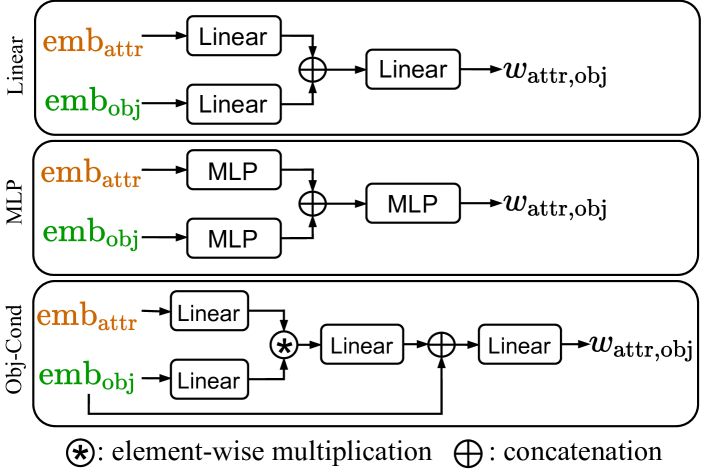
Figure 6: We show the different networks used on top of word embeddings. Empirically and following our intuition, Object-Conditioned network works best among the three (rest two are Linear and MLP). (Sec D.2)

D.3 Values for $\lambda$ and $\delta$

We find the temperature variables $\lambda$ and $\delta$ empirically. The values $\lambda=10$ and $\delta=0.05$ works best for OADis. Table 8 shows the results for all the different configurations. To understand the effect of each temperature variable, we keep all the rest of the parameters constant and only change the studied parameter.

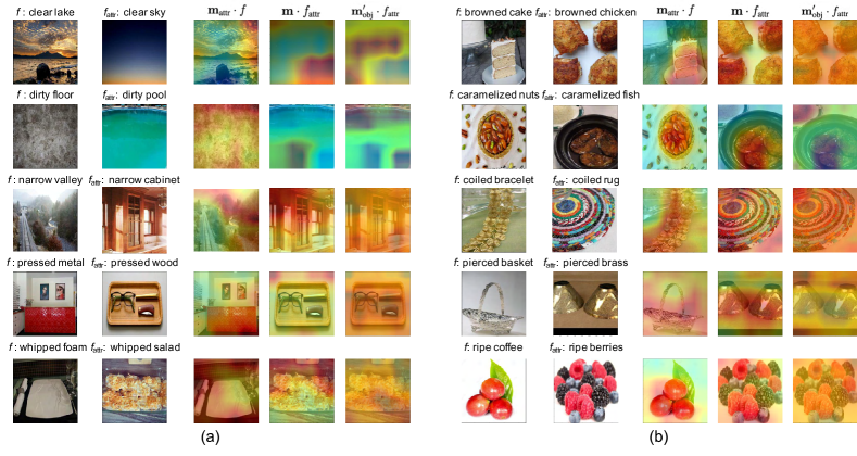
Figure 7: (a) Failure Cases: Shows the image pairs, $f$ and ${f_{\text{attr}}}$, and the similarity and dissimilarity map overlayed (details in Sec 7). Moreover, we show for some cases for MIT-States, the examples are very vague or incorrect to actually capture attribute and object concepts separately. For instance, in clear lake and clear sky, it is very difficult to distinguish lake and sky. Hence the similarity and dissimilarity maps do not perform very well. Other examples are also of failure cases where the overlayed similarity and dissimilarity maps do not make sense. (b) Correct Examples: This shows some good examples, where the similarity and dissimilarity maps capture the attibutes and objects correctly for MIT-States.

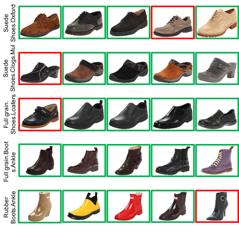
Figure 8: We show the top 5 nearest neighbors using the hallucinated unseen composition features for UT-Zappos. All the neighbors with correct labels are represented by green, whereas incorrect ones are represented with red outline.

Table 8: Results with pre-trained word-embeddings. GloVe [48] performs the best, and is therefore used for OADis. (Sec D.3)

$\lambda$	Val AUC@1	Test AUC@1
0.01	7.5	5.6
0.1	7.5	5.7
1	7.4	5.7
10	7.6	5.9
100	7.4	5.7
$\delta$	Val AUC@1	Test AUC@1
0.01	6.4	4.8
0.05	7.6	5.9
0.1	6.7	5.2

D.4 Different weights for losses

We mention different weights for each loss function in the paper, in Section 3.3. Each $\alpha$ value is empirically found, and is used in the following equation for final loss function:

$$\begin{split}\mathcal{L}&={\mathcal{L}_{\text{cls}}}+\alpha_{1}{\mathcal{L}_{\text{attr}}}+\alpha_{2}{\mathcal{L}_{\text{obj}}}+\alpha_{3}{\mathcal{L}_{\text{seen}}}+\alpha_{4}{\mathcal{L}_{\text{unseen}}}\end{split}$$

Note that ${\mathcal{L}_{\text{cls}}}$ is the main branch. The object and attribute losses are complementary, as shown in paper (Table 4). Hence, $\alpha_{1}$ and $\alpha_{2}$, which are the weights for ${\mathcal{L}_{\text{attr}}}$ and ${\mathcal{L}_{\text{obj}}}$ share the same values, i.e. 0.5. Finally, $\alpha_{4}$ and $\alpha_{5}$ have the same value since both are composition losses for seen and unseen pairs, i.e. 0.05. The chosen weights for $\alpha$ values are in bold in Table 9.

Table 9: We show empirical weights of each loss function in this table. (Sec D.4)

$\alpha_{1}$ and $\alpha_{2}$	$\alpha_{3}$ and $\alpha_{4}$	Val AUC@1	Test AUC@1
0.1	0.05	7.1	5.7
0.5	0.1	7.0	5.3
0.1	0.05	7.5	5.8
0.5	0.05	7.6	5.9
1.0	0.05	7.3	5.6

Appendix E Qualitative results

We show more qualitative results to support our architecture for different datasets.

E.1 UT-Zappos.

We show nearest neighbor results in paper for MIT-States [27] (Fig. 4(a)). Here, we show similar study for UT-Zappos [60] in Figure 8. Using the hallucinated composed features of unseen pairs, we find the top 5 nearest neighbors from test set. The red boxes show incorrect labels, where green show the correct labels.

E.2 Attention Maps

In Figure 7 and 9, we show the qualitative results on MIT-States [27] and VAW-CZSL, with examples $f$ and ${f_{\text{attr}}}$ and overlayed feature maps. To re-iterate, for images with features $f$ and ${f_{\text{attr}}}$, $\mathbf{{m_{\text{attr}}}}\cdot f$ shows how the regions in $f$ which are most similar to ${f_{\text{attr}}}$, and $\mathbf{m}\cdot{f_{\text{attr}}}$ shows the regions in ${f_{\text{attr}}}$ which are most similar to regions in $f$. Lastly, $\mathbf{{m_{\text{obj}}^{\prime}}}\cdot{f_{\text{attr}}}$ shows the regions of ${f_{\text{attr}}}$ which are most dissimilar to $f$. Although, the overlayed attention maps for similarity and dissimilarity make sense most of the times ( Figure 7(b)), due to some inconsistencies in dataset, we still find some samples where is it difficult to disentangle the attribute and object features. The main reasons why this happens is:

• Some concepts are abstract, such as clear sky, pressed metal, dirty floor (fig. 7(a)), since it is very difficult to separate dirty from floor. Hence, the attention maps for similarity and dissimilarity do not make much sense.

• Some images in MIT-States and even in other dataset are mislabelled (e.g. whipped foam in fig. 7(a)), which makes it difficult to learn attributes from those.

• Finally, for some cases, like narrow valley, our method fails to disentangle attribute and object similarity, due to various objects in the scene. For future work, using a foreground and background separator before finding similarities and dissimilarities between features can be helpful.

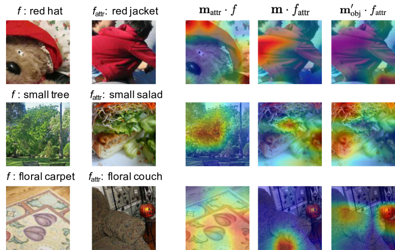
Figure 9: Correct Examples: We show the similarity and dissimilarity attention maps overlayed on images for VAW-CZSL as well. To re-iterate, for images with features $f$ and ${f_{\text{attr}}}$, $\mathbf{{m_{\text{attr}}}}\cdot f$ shows how the regions in $f$ which are most similar to ${f_{\text{attr}}}$, and $\mathbf{m}\cdot{f_{\text{attr}}}$ shows the regions in ${f_{\text{attr}}}$ which are most similar to regions in $f$. Lastly, $\mathbf{{m_{\text{obj}}^{\prime}}}\cdot{f_{\text{attr}}}$ shows the regions of ${f_{\text{attr}}}$ which are most dissimilar to $f$.

Appendix F Negative Impact of our work

Our work is a new initiative in the direction of learning visual features for objects and it’s attributes. We present it as a prototype, or an alternative direction for understanding attributes-object pairs. Similar to any other work in vision, learning attributes of objects can have various positive implications, e.g. in object detection, knowing attributes can provide additional knowledge about the objects. However, knowing the additional information about attributes, it can be used for persuasion for marketing policies, for even worse factors. Even though it seems very far fetched ideas, but using attribute classification along with object detection, knowing the attributes people can build weapons and ammunition to either counter attack the present ammunition. Attribute classification can also be used on humans, to detect certain traits of human for bypassing large-scale surveillance applications. In general, attributes provide additional information for objects, which can be used negatively or positively.

Appendix G Dataset license

Because we are creating the VAW-CZSL dataset based on the existing VAW dataset, as per the guideline of CVPR 2022, we provide the VAW dataset URL and license as follows:

• URL: https://vawdataset.com

• License: https://github.com/adobe-research/vaw_dataset/blob/main/LICENSE.md

References

- [1] Official github for c-gqa. https://github.com/ExplainableML/czsl/issues/4. Accessed: 2021-11-22.
- [2] Official github for c-gqa. https://github.com/ExplainableML/czsl/issues/3. Accessed: 2021-11-22.
- [3] Jean-Baptiste Alayrac, Josef Sivic, I. Laptev, and S. Lacoste-Julien. Joint discovery of object states and manipulation actions. 2017 IEEE International Conference on Computer Vision (ICCV), pages 2146–2155, 2017.
- [4] Y. Atzmon, F. Kreuk, U. Shalit, and Gal Chechik. A causal view of compositional zero-shot recognition. ArXiv, abs/2006.14610, 2020.
- [5] Nachwa Abou Bakr, J. Crowley, and Rémi Ronfard. Recognizing manipulation actions from state-transformations. ArXiv, abs/1906.05147, 2019.
- [6] Nachwa Abou Bakr, Rémi Ronfard, and J. Crowley. Recognition and localization of food in cooking videos. In CEA/MADiMa ’18, 2018.
- [7] Gedas Bertasius and Lorenzo Torresani. Cobe: Contextualized object embeddings from narrated instructional video, 2020.
- [8] Irving Biederman. Recognition-by-components: a theory of human image understanding. Psychological review, 94 2:115–147, 1987.
- [9] Piotr Bojanowski, Edouard Grave, Armand Joulin, and Tomas Mikolov. Enriching word vectors with subword information. Transactions of the Association for Computational Linguistics, 5:135–146, 2017.
- [10] Yu-Wei Chao, Yunfan Liu, Xieyang Liu, Huayi Zeng, and Jia Deng. Learning to detect human-object interactions. 2018 IEEE Winter Conference on Applications of Computer Vision (WACV), pages 381–389, 2018.
- [11] Chao-Yeh Chen and Kristen Grauman. Inferring analogous attributes. 2014 IEEE Conference on Computer Vision and Pattern Recognition, pages 200–207, 2014.
- [12] Hui Chen, Guiguang Ding, Xudong Liu, Zijia Lin, Ji Liu, and Jungong Han. Imram: Iterative matching with recurrent attention memory for cross-modal image-text retrieval. 2020 IEEE/CVF Conference on Computer Vision and Pattern Recognition (CVPR), pages 12652–12660, 2020.
- [13] Hui Chen, Zhixiong Nan, Jingjing Jiang, and Nanning Zheng. Learning to infer unseen attribute-object compositions. arXiv preprint arXiv:2010.14343, 2020.
- [14] Xinlei Chen, Abhinav Shrivastava, and Abhinav Gupta. NEIL: Extracting Visual Knowledge from Web Data. In IEEE International Conference on Computer Vision (ICCV), 2013.
- [15] Yunjey Choi, Youngjung Uh, Jaejun Yoo, and Jung-Woo Ha. Stargan v2: Diverse image synthesis for multiple domains. 2020 IEEE/CVF Conference on Computer Vision and Pattern Recognition (CVPR), pages 8185–8194, 2020.
- [16] Jia Deng, W. Dong, R. Socher, L. Li, K. Li, and Li Fei-Fei. Imagenet: A large-scale hierarchical image database. In CVPR 2009, 2009.
- [17] Ali Farhadi, Ian Endres, and Derek Hoiem. Attribute-centric recognition for cross-category generalization. 2010 IEEE Computer Society Conference on Computer Vision and Pattern Recognition, pages 2352–2359, 2010.
- [18] Ali Farhadi, Ian Endres, Derek Hoiem, and David Alexander Forsyth. Describing objects by their attributes. 2009 IEEE Conference on Computer Vision and Pattern Recognition, pages 1778–1785, 2009.
- [19] Alireza Fathi and James M Rehg. Modeling actions through state changes. In Proceedings of the IEEE Conference on Computer Vision and Pattern Recognition, pages 2579–2586, 2013.
- [20] Vittorio Ferrari and Andrew Zisserman. Learning visual attributes. In NIPS, 2007.
- [21] A. Fire and S. Zhu. Learning perceptual causality from video. ACM Trans. Intell. Syst. Technol., 7:23:1–23:22, 2015.
- [22] Jianlong Fu, Jinqiao Wang, Xin-Jing Wang, Yong Rui, and Hanqing Lu. What visual attributes characterize an object class? In ACCV, 2014.
- [23] Liane Gabora. The ’power of then’: The uniquely human capacity to imagine beyond the present. arXiv: Neurons and Cognition, 2015.
- [24] Kaiming He, X. Zhang, Shaoqing Ren, and Jian Sun. Deep residual learning for image recognition. 2016 IEEE Conference on Computer Vision and Pattern Recognition (CVPR), pages 770–778, 2016.
- [25] Donald D. Hoffman and Whitman Richards. Parts of recognition. Cognition, 18:65–96, 1984.
- [26] Sung Ju Hwang, Fei Sha, and Kristen Grauman. Sharing features between objects and their attributes. CVPR 2011, pages 1761–1768, 2011.
- [27] Phillip Isola, Joseph J. Lim, and E. Adelson. Discovering states and transformations in image collections. 2015 IEEE Conference on Computer Vision and Pattern Recognition (CVPR), pages 1383–1391, 2015.
- [28] Girish Kulkarni, Visruth Premraj, Vicente Ordonez, Sagnik Dhar, Siming Li, Yejin Choi, Alexander C. Berg, and Tamara L. Berg. Babytalk: Understanding and generating simple image descriptions. IEEE Trans. Pattern Anal. Mach. Intell., 35:2891–2903, 2013.
- [29] Christoph H. Lampert, Hannes Nickisch, and Stefan Harmeling. Learning to detect unseen object classes by between-class attribute transfer. 2009 IEEE Conference on Computer Vision and Pattern Recognition, pages 951–958, 2009.
- [30] Hao-Wei Lee, Chia-Po Wei, and Yu-Chiang Frank Wang. Learning grassmann manifolds for object state discovery. 2017 IEEE International Conference on Acoustics, Speech and Signal Processing (ICASSP), pages 1223–1227, 2017.
- [31] Kuang-Huei Lee, Xi Chen, Gang Hua, Houdong Hu, and Xiaodong He. Stacked cross attention for image-text matching. ArXiv, abs/1803.08024, 2018.
- [32] Kunpeng Li, Yulun Zhang, K. Li, Yuanyuan Li, and Yun Raymond Fu. Visual semantic reasoning for image-text matching. 2019 IEEE/CVF International Conference on Computer Vision (ICCV), pages 4653–4661, 2019.
- [33] Yong-Lu Li, Yue Xu, Xiaohan Mao, and Cewu Lu. Symmetry and group in attribute-object compositions. 2020 IEEE/CVF Conference on Computer Vision and Pattern Recognition (CVPR), pages 11313–11322, 2020.
- [34] Cewu Lu, Ranjay Krishna, Michael S. Bernstein, and Li Fei-Fei. Visual relationship detection with language priors. In ECCV, 2016.
- [35] Dhruv Kumar Mahajan, Sundararajan Sellamanickam, and Vinod Nair. A joint learning framework for attribute models and object descriptions. 2011 International Conference on Computer Vision, pages 1227–1234, 2011.
- [36] Massimiliano Mancini, Muhammad Ferjad Naeem, Yongqin Xian, and Zeynep Akata. Learning graph embeddings for open world compositional zero-shot learning. ArXiv, abs/2105.01017, 2021.
- [37] T. McCandless and K. Grauman. Object-centric spatio-temporal pyramids for egocentric activity recognition. In BMVC, 2013.
- [38] Tomas Mikolov, Kai Chen, Gregory S. Corrado, and Jeffrey Dean. Efficient estimation of word representations in vector space. In ICLR, 2013.
- [39] I. Misra, A. Gupta, and M. Hebert. From red wine to red tomato: Composition with context. 2017 IEEE Conference on Computer Vision and Pattern Recognition (CVPR), pages 1160–1169, 2017.
- [40] Ishan Misra*, Abhinav Shrivastava*, Abhinav Gupta, and Martial Hebert. Cross-stitch Networks for Multi-task Learning. In IEEE Conference on Computer Vision and Pattern Recognition (CVPR), 2016.
- [41] Muhammad Ferjad Naeem, Yongqin Xian, Federico Tombari, and Zeynep Akata. Learning graph embeddings for compositional zero-shot learning. ArXiv, abs/2102.01987, 2021.
- [42] Tushar Nagarajan and K. Grauman. Attributes as operators: Factorizing unseen attribute-object compositions. In ECCV, 2018.
- [43] Z. Nan, Y. Liu, N. Zheng, and S. Zhu. Recognizing unseen attribute-object pair with generative model. In AAAI, 2019.
- [44] Vicente Ordonez, Girish Kulkarni, and Tamara L. Berg. Im2text: Describing images using 1 million captioned photographs. In NIPS, 2011.
- [45] Devi Parikh and Kristen Grauman. Relative attributes. 2011 International Conference on Computer Vision, pages 503–510, 2011.
- [46] Genevieve Patterson and James Hays. Coco attributes: Attributes for people, animals, and objects. In ECCV, 2016.
- [47] Joel Pearson. The human imagination: the cognitive neuroscience of visual mental imagery. Nature Reviews Neuroscience, pages 1–11, 2019.
- [48] Jeffrey Pennington, Richard Socher, and Christopher D. Manning. Glove: Global vectors for word representation. In EMNLP, 2014.
- [49] Khoi Pham, Kushal Kafle, Zhe Lin, Zhihong Ding, Scott Cohen, Quan Tran, and Abhinav Shrivastava. Learning to predict visual attributes in the wild. In Proceedings of the IEEE/CVF Conference on Computer Vision and Pattern Recognition (CVPR), 2021.
- [50] Senthil Purushwalkam, Maximilian Nickel, Abhinav Gupta, and Marc’Aurelio Ranzato. Task-driven modular networks for zero-shot compositional learning. 2019 IEEE/CVF International Conference on Computer Vision (ICCV), pages 3592–3601, 2019.
- [51] Alec Radford, Jong Wook Kim, Chris Hallacy, Aditya Ramesh, Gabriel Goh, Sandhini Agarwal, Girish Sastry, Amanda Askell, Pamela Mishkin, Jack Clark, Gretchen Krueger, and Ilya Sutskever. Learning transferable visual models from natural language supervision. CoRR, abs/2103.00020, 2021.
- [52] Aditya Ramesh, Mikhail Pavlov, Gabriel Goh, Scott Gray, Chelsea Voss, Alec Radford, Mark Chen, and Ilya Sutskever. Zero-shot text-to-image generation. CoRR, abs/2102.12092, 2021.
- [53] Liyue Shen, Serena Yeung, Judy Hoffman, Greg Mori, and Li Fei-Fei. Scaling human-object interaction recognition through zero-shot learning. 2018 IEEE Winter Conference on Applications of Computer Vision (WACV), pages 1568–1576, 2018.
- [54] Abhinav Shrivastava, Saurabh Singh, and Abhinav Gupta. Constrained semi-supervised learning using attributes and comparative attributes. In European Conference on Computer Vision, 2012.
- [55] Tiancai Wang, Tong Yang, Martin Danelljan, Fahad Shahbaz Khan, X. Zhang, and Jian Sun. Learning human-object interaction detection using interaction points. 2020 IEEE/CVF Conference on Computer Vision and Pattern Recognition (CVPR), pages 4115–4124, 2020.
- [56] Kun-Juan Wei, Muli Yang, H. Wang, Cheng Deng, and Xianglong Liu. Adversarial fine-grained composition learning for unseen attribute-object recognition. 2019 IEEE/CVF International Conference on Computer Vision (ICCV), pages 3740–3748, 2019.
- [57] Guangyue Xu, Parisa Kordjamshidi, and Joyce Yue Chai. Zero-shot compositional concept learning. ArXiv, abs/2107.05176, 2021.
- [58] Ziwei Xu, Guangzhi Wang, Yongkang Wong, and Mohan S. Kankanhalli. Relation-aware compositional zero-shot learning for attribute-object pair recognition. ArXiv, abs/2108.04603, 2021.
- [59] Muli Yang, Cheng Deng, Junchi Yan, Xianglong Liu, and Dacheng Tao. Learning unseen concepts via hierarchical decomposition and composition. 2020 IEEE/CVF Conference on Computer Vision and Pattern Recognition (CVPR), pages 10245–10253, 2020.
- [60] A. Yu and K. Grauman. Fine-grained visual comparisons with local learning. 2014 IEEE Conference on Computer Vision and Pattern Recognition, pages 192–199, 2014.