Fine-resolution landscape-scale biomass mapping using a spatiotemporal patchwork of LiDAR coverages

Abstract

Estimating forest aboveground biomass (AGB) at large scales and fine spatial resolutions has become increasingly important for greenhouse gas accounting, monitoring, and verification efforts to mitigate climate change. Airborne LiDAR is highly valuable for modeling attributes of forest structure including AGB, yet most LiDAR collections take place at local or regional scales covering irregular, non-contiguous footprints, resulting in a patchwork of different landscape segments at various points in time. Here, as part of a statewide forest carbon assessment for New York State (USA), we addressed common obstacles in leveraging a LiDAR patchwork for AGB mapping at landscape scales, including selection of training data, the investigation of regional or coverage specific patterns in prediction error, and map agreement with field inventory across multiple scales.

Three machine learning algorithms and an ensemble model were trained with Forest Inventory and Analysis (FIA) field measurements, airborne LiDAR, and topographic, climatic, and cadastral geodata. Using a novel set of plot selection criteria and growth adjustments to temporally align LiDAR coverages with FIA measurements, 801 FIA plots were selected with co-located point clouds drawn from a patchwork of 17 leaf-off LiDAR coverages (2014-2019). Our ensemble model was used to produce 30 m AGB prediction surfaces within a predictor-defined area of applicability (98% of LiDAR coverage) and within four vegetated landcover classes. The resulting AGB maps were compared with FIA plot-level and areal estimates at multiple scales of aggregation. Our model was overall accurate (% root mean squared error 22-45%; mean absolute error 11.6-29.4 Mg ha^-1; mean error 2.4-6.3 Mg ha^-1), explained 73-80% of field-observed variation, and yielded estimates that were largely consistent with FIA’s design-based estimates (89% of estimates within FIA’s 95% confidence interval). We share practical solutions to challenges faced in using spatiotemporal patchworks of LiDAR to meet growing needs for AGB prediction and mapping in support of broad-scale applications in forest carbon accounting and ecosystem stewardship.

Keywords Airborne LiDAR  $\cdot$ Aboveground biomass  $\cdot$ Machine learning  $\cdot$ Model ensembles  $\cdot$ Forest Inventory and Analysis (FIA)

1 Introduction

Mapping and monitoring forest aboveground biomass (AGB) has become increasingly important as the basis for large-scale accounting of carbon and greenhouse gas (GHG) fluxes in support of policy, regulatory, and land stewardship initiatives to mitigate global climate change. Although carbon stocks are the ultimate endpoint in GHG accounting, for several practical reasons forest AGB serves as a proxy for carbon stocks (and stock-changes) in large-scale accounting methodologies (Buendia et al. 2019; Woodall et al. 2015). Such applications, based primarily on field inventory, yield aggregate tabular estimates for political units (e.g., states, provinces), but offer little insights on landscape patterns within and across those units. Landscape-scale AGB maps with fine-resolutions can serve as inputs to GHG accounting and can help decision makers identify specific units of land for protection from deforestation, or as suitable candidates for reforestation, afforestation, or improved management in efforts to increase terrestrial carbon sequestration and offset GHG emissions from other sectors (R. A. Houghton et al. 2012; R. Houghton 2005).

National field sampling programs, like the United States Department of Agriculture’s Forest Inventory and Analysis program (FIA) (Gray et al. 2012), provide estimates of AGB at individual plots and are scaled to larger areas through a design-based approach (Bechtold and Patterson 2005). However, the resolution at which design-based estimates can be reliably produced is limited to relatively coarse units, such as states or counties, due to the density of the sample (McRoberts 2011). For instance, the FIA program samples forest conditions and land cover across New York State (NYS) at a density of roughly one plot per 2,400 ha (Gray et al. 2012), while 65% of NY forestlands are owned in parcels smaller than 40 ha (L’Roe and Allred 2013). Although FIA’s extensive plot network was never designed to yield such localized results, this inherent resolution mismatch poses obstacles to accounting and decision-support applications that must account for local geography, both ecological and cadastral, to be practical and effective.

To address this need, model-based approaches combining field inventory data, like the FIA, with auxiliary remotely sensed data can produce predictions for all map units (pixels) in a given area. Airborne LiDAR has been established as a highly valuable remotely sensed data source for such purposes (Huang et al. 2019; Hurtt et al. 2019; Chen and McRoberts 2016) offering detailed information on forest structure at fine spatial resolutions. However, LiDAR data are most commonly acquired at local to regional scales in irregular or non-contiguous footprints (Skowronski and Lister 2012), resulting in a complex patchwork of data from component coverages acquired at different times with different sensors and mission parameters, in turn posing a host of challenges for broad-scale AGB mapping (Lu et al. 2014; Huang et al. 2019). These challenges include insufficient field inventory plots that spatially and temporally match LiDAR acquisitions and data discrepancies among LiDAR coverages.

Yet several groups have undertaken broad-scale AGB mapping efforts with LiDAR patchworks with varying degrees to which training data have been pooled from multiple LiDAR coverages. The choice between an individual or a pooled modeling approach often reflects practical considerations relating to sufficient sample size across all sub-regions and the cost of developing multiple models. Nilsson et al. (2017) did not pool at all, implementing a separate model trained for each coverage. Huang et al. (2019) pooled by ecoregion. Both Ayrey et al. (2021) and Hauglin et al. (2021) pooled all coverages but used a convolutional neural network and a mixed-effects model respectively, with differing protocols for inventory plot selection.

In this study, as part of a broader effort for map-based forest carbon accounting across NYS, we addressed several common challenges in using LiDAR patchworks for broad-scale, fine-resolution biomass modeling and mapping. We leveraged FIA inventories for model training and assessment data, and implemented FIA-developed methods to assess the agreement between our estimates and those produced by FIA. With the goal of producing a spatially explicit representation of FIA AGB information, we used a model-based approach to translate FIA’s discrete plot-level estimates to wall-to-wall predictions at a 30 m resolution across a patchwork of 17 discrete LiDAR coverages in NYS.

We implemented a rigorous plot selection framework to limit temporal lags between LiDAR acquisitions and field inventories. When strict temporal alignment yielded too few plots, we leveraged repeated FIA inventories to boost the number of plots that temporally match LiDAR acquisitions without the incorporation of additional models or manual processes (Ayrey et al. 2021; Hauglin et al. 2021). In spite of this strategy, we were left with limited model training data, where some coverages and regions lacked sufficient information to support independent models, necessitating a single model or pooled approach.

We used machine learning (ML) algorithms including random forests (Breiman 2001a), gradient boosting machines (Friedman 2002), and support vector machines (Cortes and Vapnik 1995), as well as ‘stacked ensembles’ of said algorithms (Wolpert 1992). These have been shown to be better suited for pure prediction (Efron 2020; Breiman 2001b) when compared to their conventional regression counterparts (Hauglin et al. 2021), especially when the input data are noisy and the processes governing the relationships between predictors and responses are complex or unknown, as is often the case in nature (Wintle et al. 2003). Furthermore, using pre-selected hyperparameters these algorithms can be trained in minutes with typical consumer-grade hardware, avoiding some of the drawbacks of computationally intense deep-learning approaches (Ayrey et al. 2021).

We also employed multiple strategies to address concerns that differences among sensors and mission parameters could lead to non-randomly distributed errors in our AGB prediction surfaces. First, we produced an area of applicability (Meyer and Pebesma 2021) mask to both examine the uniformity of our predictors across the component coverages, as well as to screen predictions based on anomalous predictor data. Second, we examined the spatial autocorrelation of our residuals and mapped our prediction error to identify the presence of region or coverage specific patterns. Finally, we assessed the agreement between our mapped predictions and FIA estimates across a range of scales (Riemann et al. 2010; Menlove and Healey 2020).

2 Data and Methods

2.1 LiDAR Coverages

Our study relied upon a set of 17 LiDAR datasets hosted by the NYS GIS Program Office (GPO) covering 62.46% (7,835,690 ha) of NYS (hereafter “GPO-LiDAR area”; Table 1; Figure 1). We selected individual coverages from the most recent five years of available data that contained temporally matching field data (2014-2019) to minimize sensor and data differences. All component coverages were originally collected to generate digital elevation models for flood risk analysis, and to this end were flown during leaf-off conditions. Several previous studies have shown that leaf-off LiDAR models can be as accurate as their leaf-on counterparts (Hawbaker et al. 2010; White et al. 2015; Anderson and Bolstad 2013).

Table 1: Component LiDAR coverage metadata. IDs for cross figure correspondence; Year of acquisition; Area covered (ha); Pulse density (PD) in pulses per m²; Number of FIA plots in model and map assessment datasets. Area of Applicability (AOA) in percent of LiDAR coverage pixels considered inside of the area of applicability. AOA computation conducted after initial LCMAP masking.

ID	Coverage Name	Year	Area	PD	% AOA	Model	Assessment
1	Erie, Genesee & Livingston	2019	555,853	2.04	97.72	11	33
2	Fulton, Saratoga, Herkimer & Franklin	2018	557,421	2.60	99.61	39	84
3	Southwest B	2018	527,075	1.98	98.06	28	66
4	Cayuga & Oswego	2018	438,201	2.78	96.89	25	43
5	Southwest	2017	423,714	1.98	98.53	33	74
6	Franklin & St. Lawrence	2017	977,620	2.69	99.24	104	188
7	Oneida Subbasin	2017	264,886	2.10	96.02	15	31
8	Allegany & Steuben	2016	309,081	1.69	97.77	32	53
9	Columbia & Rensselaer	2016	248,839	1.69	98.19	17	28
10	Clinton, Essex & Franklin	2015	600,755	2.23	98.70	115	127
11	Warren, Washington & Essex	2015	611,704	3.24	99.37	106	128
12	Madison & Otsego	2015	471,564	2.13	99.24	56	92
13	3 County	2014	755,629	2.04	96.12	92	114
14	Long Island	2014	315,542	2.04	94.77	22	12
15	Schoharie	2014	256,464	2.04	95.12	31	40
16	New York City (NYC)	2014	77,211	1.54	90.40	2	1
17	Great Lakes	2014	444,215	2.04	98.47	73	103
	GPO-LiDAR		7,835,773		98.12	801	1,217

Figure 1: GPO-LiDAR component coverages, colored by year of acquisition and labeled by ID numbers in Table 1.

2.2 Field Data

Two field datasets were compiled from the inventory USDA FIA inventory in NYS with the distinct purposes of model development and map assessment. The FIA program compiled AGB estimates for trees $\geq$ 12.7 cm (5 in) diameter at breast height (Gray et al. 2012), and were converted to units of megagrams per hectare (Mg ha^-1). The FIA uses permanent inventory plots arranged in a quasi-systematic hexagonal grid that are remeasured on a rolling seven-year basis in the Northeastern United States (Bechtold and Patterson 2005). Tree measurements, and subsequently AGB estimates, are only recorded on portions of plots considered forested. For an area to be considered forested by the FIA, the area must be at least 10% stocked with trees, at least 0.4 ha (1 acre) in size, and at least 36.58 m (120 ft) wide. Additionally, any lands meeting these minimum requirements, but developed for nonforest land uses, are not considered forested. With an understanding that some nonforest conditions contained AGB that was not measured by FIA, we assumed that any nonforest condition contained 0 AGB.

FIA plots are composed of four identical circular subplots with radii of 7.32 m (24 ft), with one subplot centered at the macroplot centroid and three subplots located 36.6 m (120 ft) away at azimuths of 360^∘, 120^∘, and 240^∘ (Bechtold and Patterson 2005). The plot locations were provided by the FIA program in the form of average coordinates, collected over multiple repeat visits, representing the centroid of the center subplot, which we then used to build a polygon dataset representing the entire plot layout including all four subplots (Figure 2). Averaged coordinates were necessary due to the lack of precision of initial GPS coordinates for the macroplot centroids (Hoppus and Lister 2005). Any reference to an FIA plot hereafter implies the aggregation of all four component subplots.

2.2.1 Model Development Dataset

In selecting plots for model development (model dataset hereafter; Table 1) we aimed to maximize the number of reference plots (Fassnacht et al. 2014), while minimizing the temporal lag between LiDAR acquisitions and inventories and ensuring high quality co-registered LiDAR data (White et al. 2013; CEOS 2021). Temporal misalignment between plots and LiDAR has been shown to introduce error in model predictions; Gonçalves et al. (2017) found that 7-17% of their prediction error could be attributed to 3-year lags between inventories and LiDAR acquisitions.

We only considered FIA plots when all subplots were marked as measured and when forest conditions were uniform at the plot level (all subplots completely forested or completely non-forested). Only 324 plots were available when we required a strict temporal match between inventories and LiDAR acquisitions (Table 2; Criterion 1). To increase the number of reference plots, we applied a growth adjustment to FIA plots with inventories both before and after the LiDAR acquisition, or ‘bracketing inventories’. For plots with bracketing inventories, we excluded those where AGB decreased by $\geq$ 5% between measurements indicating a disturbance event on the plot. For the remaining (relatively undisturbed) plots with bracketing inventories, AGB at the time of the LiDAR collection was then estimated by linearly interpolating between bracketing FIA estimates. This procedure added 843 plots to our dataset (Table 2; Criterion 2), and is analogous to existing growth adjustment methods (Gonçalves et al. 2017; Gobakken and Næsset 2008).

Several plot exclusion rules were implemented to filter duplicates and remove problematic observations resulting from vegetation in non-forest conditions, interfering structures, or other data anomalies which would otherwise degrade the relationships between AGB and our predictor variables (Table 2; Criteria 3-5). Point clouds were clipped to the constructed plot footprints and were excluded with criteria 3-5 (Figure 2).

2.2.2 Map Assessment Dataset

For our map assessment dataset (assessment dataset hereafter; Table 1) we were primarily concerned with maintaining FIA’s probability sample of inventory plots in order to leverage unbiased estimators of map agreement metrics (Stehman and Foody 2019; Riemann et al. 2010). As in the model dataset, only those plots with all four subplots marked as measured were considered. Excluding non-measured plots, however, does not invalidate FIA’s probability sample, as the FIA program assumes these plots to be randomly distributed across the landscape (Bechtold and Patterson 2005). To this end, we selected FIA plots on a coverage-by-coverage basis (Figure 1), choosing only plots that had been inventoried in +/- 2 years from the year of the LiDAR acquisition, but not inventoried in the same year as the LiDAR acquisition to maintain independence from the model dataset (Table 3; Criterion 1). Where plots were shared with the model dataset, AGB values differed, with AGB values derived from measurements in the map assessment dataset, and AGB values derived from our growth-adjustment process in the model dataset, therefore representing different points in time. Furthermore, plots falling outside of our mapped area, based on our landcover and area-of-applicability masks (Section 2.6), were excluded as they were considered outside our population of interest (Table 3; Criteria 2-3).

Table 2: Summary of plot selection criteria for the model dataset.

	Criteria	Description	Num Plots
	1	Plots inventoried in the same year as a LiDAR acquisition.	324
Include	2	Plots growth-adjusted to temporally align with LiDAR acquisition.	843
	3	Plots where measured AGB = 0 Mg ha-1 but maximum LiDAR return $>$ 1m.	327
	4	Plots where the convex hull of LiDAR returns clipped to a given subplot did not contain at least 90% of the subplot area.	13
Exclude	5	Plots duplicated in neighboring coverages. Temporal matches given preference, followed by inventory recency.	26

Table 3: Summary of plot selection criteria for the assessment dataset.

	Criteria	Description	Num Plots
Include	1	Plots inventoried in +/- 2 years of LiDAR acquisition but not in the same year as the acquisition.	1639
	2	Plots with any portion of the plot footprint outside of our landcover mask.	291
Exclude	3	Plots with any portion of the plot footprint outside of our area of applicability mask.	131

2.3 LiDAR and Auxiliary Data Pre-Processing

First, we height-normalized the raw LiDAR data and computed 40 predictors (Supplementary Materials S1) based on previous studies (Hawbaker et al. 2010; Huang et al. 2019; Pflugmacher et al. 2014). Predictors at individual FIA plots were computed from LiDAR returns clipped to only the measured subplot footprints and then pooled at the plot level (Figure 2). The corresponding predictors computed for map pixels were based on the set of returns within each 30 m cell. The lidR (Roussel and Auty 2020; Jean-Romain et al. 2020) package in R (R Core Team 2021) was used for height-normalization and predictor generation.

A group of steady-state predictors was included to represent geospatial variation in climate and topography (Kennedy et al. 2018). Additionally, a 2019 tax parcel layer was incorporated as a set of boolean indicator variables (Supplementary Materials S2). Tax codes and categories provide cadastral information related to land-use and management (Thompson et al. 2011). All auxiliary predictors were reprojected and resampled to pixel geometries matching the 30 m LiDAR predictor surfaces.

Figure 2: a) FIA plot layout overlaid on a 1 m LiDAR-derived max-height surface. b) Height-normalized LiDAR returns clipped to individual FIA subplots and pooled prior to predictor computation.

2.4 Model Development

Three ML models were fit to a randomly selected 80% of the model dataset (training set; n = 630), leaving the 20% remaining plots as an independent testing set to assess the final model performance on point clouds clipped to FIA plot footprints (testing set; n = 171). Random forest models (RF; ranger; Wright and Ziegler (2017)), stochastic gradient boosting machines (GBM; lightgbm; Ke et al. (2021), Ke et al. (2017)), and support vector machines (SVM; kernlab; Karatzoglou et al. (2004)) were tuned using the 80% training dataset and an iterative grid search approach, starting by testing wide ranges of hyperparameters using five-fold cross validation and then narrowing down to only the most performant combinations over several iterations. Models then used the most accurate sets of hyperparameters in all other analyses. For each of the $n$ observation in the training dataset, all three component models were fit, using their optimal hyperparameters, with $n-1$ observations. Predictions for each component model were made for the nth (left out) observation. A linear regression model was used to estimate AGB as a function of these leave-one-out predictions, combining the three ML approaches in a stacked ensemble to reduce the generalization error of our component models (Wolpert 1992).

2.5 Model Performance

Model performance was assessed against the 20% testing partition of the model dataset (Table 1) based on metrics including root-mean-squared error in Mg ha^-1 (RMSE, equation (1)), percent RMSE (% RMSE, equation (2)), mean absolute error in Mg ha^-1 (MAE, equation (3)), percent MAE (% MAE, equation (4)), mean error in Mg ha^-1 (ME, equation (5)), and the coefficient of determination ($R^{2}$, equation (6)) as follows:

$$\operatorname{RMSE}=\sqrt{(\frac{1}{n})\sum_{i=1}^{n}(y_{i}-\hat{y_{i}})^{2}}$$ (1)

$$\operatorname{\%\ RMSE}=100\cdot\frac{\operatorname{RMSE}}{\bar{y}}$$ (2)

$$\operatorname{MAE}=(\frac{1}{n})\sum_{i=1}^{n}(\lvert y_{i}-\hat{y_{i}}\rvert)$$ (3)

$$\operatorname{\%\ MAE}=100\cdot\frac{\operatorname{MAE}}{\bar{y}}$$ (4)

$$\operatorname{ME}=(\frac{1}{n})\sum_{i=1}^{n}(y_{i}-\hat{y_{i}})$$ (5)

$$\operatorname{R^{2}}=1-\frac{\sum_{i=1}^{n}\left(y_{i}-\hat{y}_{i}\right)^{2}}{\sum_{i=1}^{n}\left(y_{i}-\bar{y}\right)^{2}}$$ (6)

where $n$ is the number of FIA plots included in the data set, $\hat{y_{i}}$ is the predicted value of AGB, $y_{i}$ the AGB value measured at the corresponding location, and $\bar{y}$ the mean AGB value from FIA field measurements.

Standard errors for R² and RMSE were computed as follows:

$$\operatorname{SE_{boot}}=\sqrt{\frac{Var_{boot}}{n}}$$ (7)

where $n$ is the number of FIA plots included in the dataset, and $Var_{boot}$ is computed as the variance of R² and RMSE estimates for 1000 iterations of bootstrap resampling. Standard errors for MAE and ME were computed as follows:

$$\operatorname{SE}=\sqrt{\frac{\sum_{i=1}^{n}\left(e_{i}-\bar{e}\right)^{2}}{n-1}}$$ (8)

where $e_{i}$ is the error at an FIA plot, and $\bar{e}$ is the mean error from all FIA plots included. In the case of MAE, $e_{i}=|y_{i}-\hat{y_{i}}|$, the absolute value of the error at a given FIA plot.

2.6 AGB Mapping and Post-processing

The linear model ensemble was used to make predictions for all 30 m pixels within the GPO-LiDAR area. Predictions on newer coverages superseded those based on older coverages in areas where neighboring LiDAR coverages overlapped. All AGB prediction surfaces were projected to match Landsat 30 m pixel geometries to avoid mixed pixel effects in subsequent raster overlay analyses (Wulder et al. 2022).

With recognition that our predictions are best suited to areas populated by woody biomass, we tabulated our predictions across landcover types determined from the United States Geological Survey’s Land Change Monitoring, Assessment, and Projection (LCMAP) primary classification products (Brown et al. 2020; Zhu and Woodcock 2014), which has a reported overall accuracy of 77.4% in the eastern United States for the years 1985-2018 (Pengra et al. 2020). LCMAP’s annual resolution (1985-2019) allowed for temporal alignment with the patchwork of LiDAR-AGB surfaces, and shared identical pixel geometries. We masked our AGB prediction surfaces to remove Developed, Water, and Barren pixels, and then tabulated AGB by the four remaining vegetated LCMAP classes of Tree Cover, Grass/Shrub, Cropland, and Wetland.

Lastly, we computed an area of applicability (AOA) surface which identifies pixels containing predictor data that are beyond a pre-specified predictor-space distance from the training data (Meyer and Pebesma (2021); Supplementary Materials S4). We used this surface as a final mask for our AGB prediction surfaces, restricting our maps to only areas that were well-represented in the training data.

2.7 Map Agreement Analysis

We assessed the agreement between our AGB maps and FIA reference data following approaches prescribed by Riemann et al. (2010) and Menlove and Healey (2020). The former evaluated agreement across a range of scales and accounts for the mismatch in spatial support between map aggregate estimates (many pixels) and FIA aggregate estimates (few plots) by only extracting pixels coincident with FIA plots. The latter compared FIA-derived AGB estimates — which have been adjusted for forest cover within, and area-extrapolated to, hexagon map units — to zonal averages of our mapped AGB.

Following Riemann et al. (2010) we compared our AGB prediction surfaces to the assessment dataset (Section 2.2). Comparisons were made at both the plot-to-pixel scale and within variably-sized hexagons with distances between centroids ranging from 10 km (8660 ha) to 100 km (866,025 ha). As an extension of the Riemann et al. (2010) methodology we assessed prediction error (RMSE, MAE, ME) with choropleth maps that summarized the mapped residuals and FIA reference data distributions within hexagon units with centroids spaced 50 km apart. We also grouped plot to pixel results by the majority LCMAP classification at each plot, to demonstrate the level of agreement across vegetated landcover classes. To evaluate the presence of spatial autocorrelation among mapped residuals, which could indicate the presence of regional or coverage specific error in our model’s predictions, Global Moran’s I statistics were computed for search radii ranging from 1 to 50 km using both the model dataset and the assessment dataset separately (Moran 1950).

Following the Menlove and Healey (2020) approach we compared the average of our masked predictions, weighted by the proportion of each pixel intersecting a given hexagon, to a set of FIA-derived estimates for 64,000 ha hexagons representing FIA’s finest acceptable scale for the most recent inventory cycle in NYS (2013-2019) (Menlove and Healey 2020). As recommended by Menlove and Healey (2020), we accounted for differences in forest definitions between the FIA estimates and our mapped estimates by dividing FIA estimates by the total area of vegetated (based on LCMAP Tree cover, Wetland, Cropland, Grass/Shrub) pixels within each hexagon. Lastly, we limited this comparison to only those hexagons that contained > 10% mapped area, using the summed area of all pixels inside of our LCMAP and AOA mask (Section 2.6) to define mapped area within each hexagon.

The exactextractr (Daniel Baston 2021), spdep (Bivand, Pebesma, and Gomez-Rubio 2013), sf (Pebesma 2018), raster (Hijmans 2021), and terra (Hijmans 2022) packages in R (R Core Team 2021) were used to conduct all analyses described here. Further description of this assessment is included in Supplementary Materials S5.

3 Results

3.1 Growth-Adjusted Field Plots

Of the 801 FIA plots in our model dataset, 562 were growth-adjusted, representing about 70% of the full dataset. The average annual AGB increment applied to all growth-adjusted plots was 1.84 Mg ha^-1 year^-1 over an average of 3.96 years. The largest annual AGB increment applied was 11.17 Mg ha^-1 year^-1 over 3 years. The longest adjustments (applied to 5 plots) occurred over 10 years at an average annual increment of 2.63 Mg ha^-1 year^-1.

3.2 Model Performance

The final model performance against the 20% test partition of the model dataset showed generally accurate predictions, but with greater accuracy towards the mean of the reference distribution (Figure 3). This resulted in slight overpredictions at smaller AGB plots and underpredictions at larger AGB plots (Figure 3). A more detailed analysis of performance for the ensemble model and the three component models can be found in Supplementary Materials S3.

Figure 3: Measured vs predicted AGB scatter plot for the testing portion of the model dataset. AGB values in Mg ha^-1. GMFR trend line shown with dashed (orange) line, and 1:1 line shown with solid (red) line

3.3 AGB by Landcover Class

Approximately 62% of all pixels, accounting for 87% of the total mapped AGB (Figure 4), were contained within areas identified as Tree cover by LCMAP (Table 4). All other LCMAP classes contained comparatively small, but non-zero estimates of AGB, with Wetlands and Grass/Shrub containing larger average predictions within small portions of the mapped area, and Cropland containing smaller average predictions across a larger proportion of the mapped area (Table 4).

Figure 4: AGB prediction surfaces reflecting a temporal patchwork of conditions across the 17 component LiDAR coverages in the GPO-LiDAR area with New York State (USA).

Table 4: Summary of FIA reference plots in the model dataset and mapped predictions by LCMAP landcover classes. n = number of plots. Mean AGB values in Mg ha^-1. Total AGB values in millions of metric tons. Area in hectares. AOA expressed as percent of LCMAP classified pixels considered inside of the area of applicability.

	Reference Plots		Mapped
LCMAP	n	Mean AGB	Area	% Area	Mean AGB	Total AGB	% AGB	% AOA
Tree cover	599	137.97	4,251,812	62.42	132.66	564.06	87.38	98.13
Cropland	132	1.98	1,748,905	25.68	14.11	24.67	3.82	98.25
Wetland	36	115.13	613,578	9.01	77.22	47.38	7.34	97.64
Grass/Shrub	12	30.68	196,852	2.89	47.86	9.42	1.46	98.17

3.4 Area of Applicability

All mapped (vegetated) LCMAP classes contained AOA $\geq$ 97.64% and the AOA breakdown across component LiDAR coverages (after LCMAP masking) was uniform ($\geq$ 90.4%) with NYC and Long Island the only two coverages with $\leq$ 95% AOA (Tables 1 and 4). In total, 98.12% of the GPO-LiDAR area was considered inside the AOA after initial LCMAP masking.

3.5 Map Agreement Analysis

We observed improved agreement between the mapped estimates and the FIA estimates as the aggregation unit size increased, with % RMSE decreasing from 45 to 15% and MAE decreasing from 28 to 10 Mg ha^-1 (Table 5, Figures 5 and 6). The scatter plot results (Figure 5) for the plot to pixel and 10 km scales show a pattern of large overpredictions where FIA reference values are 0 Mg ha^-1 AGB — likely an indication of the structural zeroes introduced by FIA’s strict definition of forest. Notably, ME increased as a function of aggregation unit size, which appears to be a reflection of outlier hexagons with very small samples rather than any additive effects from aggregation (Supplementary materials S5). We again observed less accurate predictions at the extremes of the distributions across most scales, though our extreme predictions (small and large) became more accurate as a function of aggregation unit size, as indicated by the geometric mean functional relationship (GMFR; Riemann et al. (2010)) slope approaching 1 at the largest scales (Figures 5 and 6).

The model’s mapped residuals grouped to 50 km spaced hexagons did not reveal any observable spatial patterns of prediction error (RMSE, MAE, ME) (Figure 7). The ME map (Figure 7c) was dominated by near-zero positive prediction error but indicated the tendency for hexagons with negative prediction ME to have larger mean FIA AGB values, while hexagons with positive ME were more likely to have smaller mean FIA AGB values (Figure 7g). The RMSE map (Figure 7a) and MAE map (Figure 7b) largely mirrored one another.

Comparison of our AGB maps with FIA’s design based estimates of AGB density (Menlove and Healey 2020) indicated overall strong agreement, with 89% of our estimates falling within the FIA estimate 95% confidence intervals (CI) (Figure 8). The majority of our estimates falling outside the CI were at the lower range of the AGB distribution, reinforcing the observed pattern of overprediction in comparison to FIA-derived estimates at the low end of the reference distribution.

Map agreement across LCMAP vegetated classes was highly variable, with the smallest % RMSE for plots classified as Tree Cover by LCMAP (Table 6). Absolute RMSE for Grass/Shrub and Cropland plots was small (< 24 Mg ha^-1), but their relative values were quite large (% RMSE > 100%), reflecting the small FIA AGB averages within these classes. Mean errors were positive and large for Grass/Shrub and Croplands (14.64 Mg ha^-1 and 6.67 Mg ha^-1 respectively; Table 6), suggesting that errors contained in these two landcover classes had a relatively large contribution to the overall patterns of positive ME and overprediction on the low end of the FIA AGB distribution across the entire GPO-LiDAR area.

The global Moran’s I analysis with the assessment dataset found evidence of very weak spatial autocorrelation ($\leq$ 0.10) in mapped residuals for all search radii (Supplementary Materials S6). Notably, when the analysis was conducted with the model dataset, similarly very weak spatial autocorrelation ($\leq$ 0.08) was only evident for search radii of 9 km to 14 km, but was not evident at any other scales (Supplementary Materials S6).

Table 5: Map agreement results for select scales. Distance = distance between hexagon centroids in km; PPH = plots per hexagon; n = number of comparison units (plots or hexagons); RMSE, MAE, ME in Mg ha^-1. All accuracy metrics as defined in Section 2.5. Standard errors in parentheses.

Distance	n	PPH	% RMSE	RMSE	MAE	ME	R2
	1217		44.87	40.93 (0.04)	28.12 (0.85)	4.40 (1.17)	0.73 (0.01)
10	739	1.65	37.95	34.06 (0.05)	23.95 (0.89)	4.63 (1.24)	0.77 (0.01)
25	199	6.12	27.95	24.68 (0.13)	17.13 (1.26)	2.36 (1.75)	0.80 (0.01)
50	72	16.9	25.86	21.17 (0.41)	14.26 (1.86)	6.26 (2.40)	0.78 (0.01)
100	26	46.81	22.28	17.39 (0.71)	11.58 (2.59)	5.42 (3.30)	0.74 (0.03)

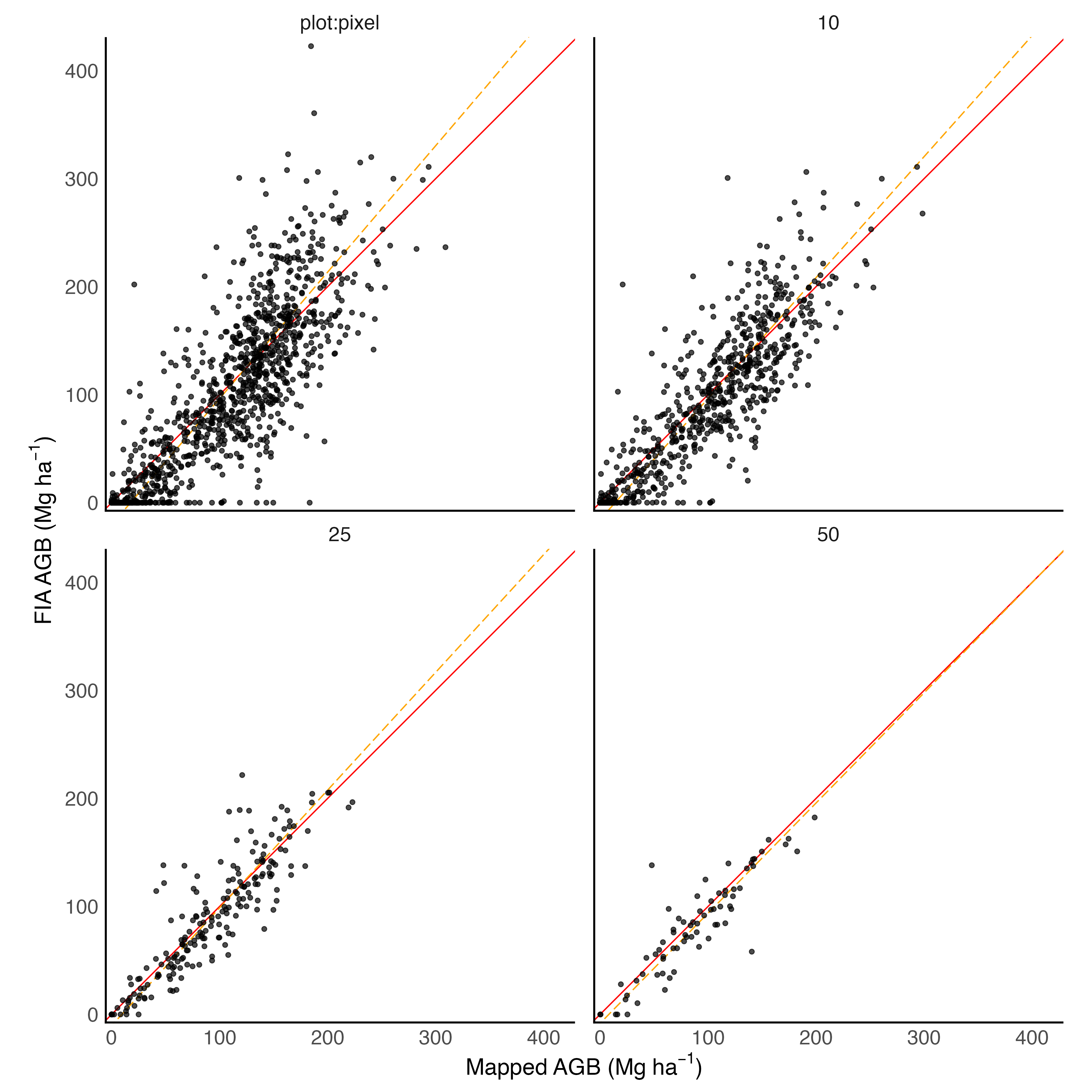
Figure 5: Comparing mapped AGB to FIA estimated AGB across selected scales represented by distances between hexagon centroids (plot:pixel, 10 km, 25 km, and 50 km). AGB values in Mg ha^-1. GMFR trend line shown with dashed (orange) line, and 1:1 line shown with solid (red) line.

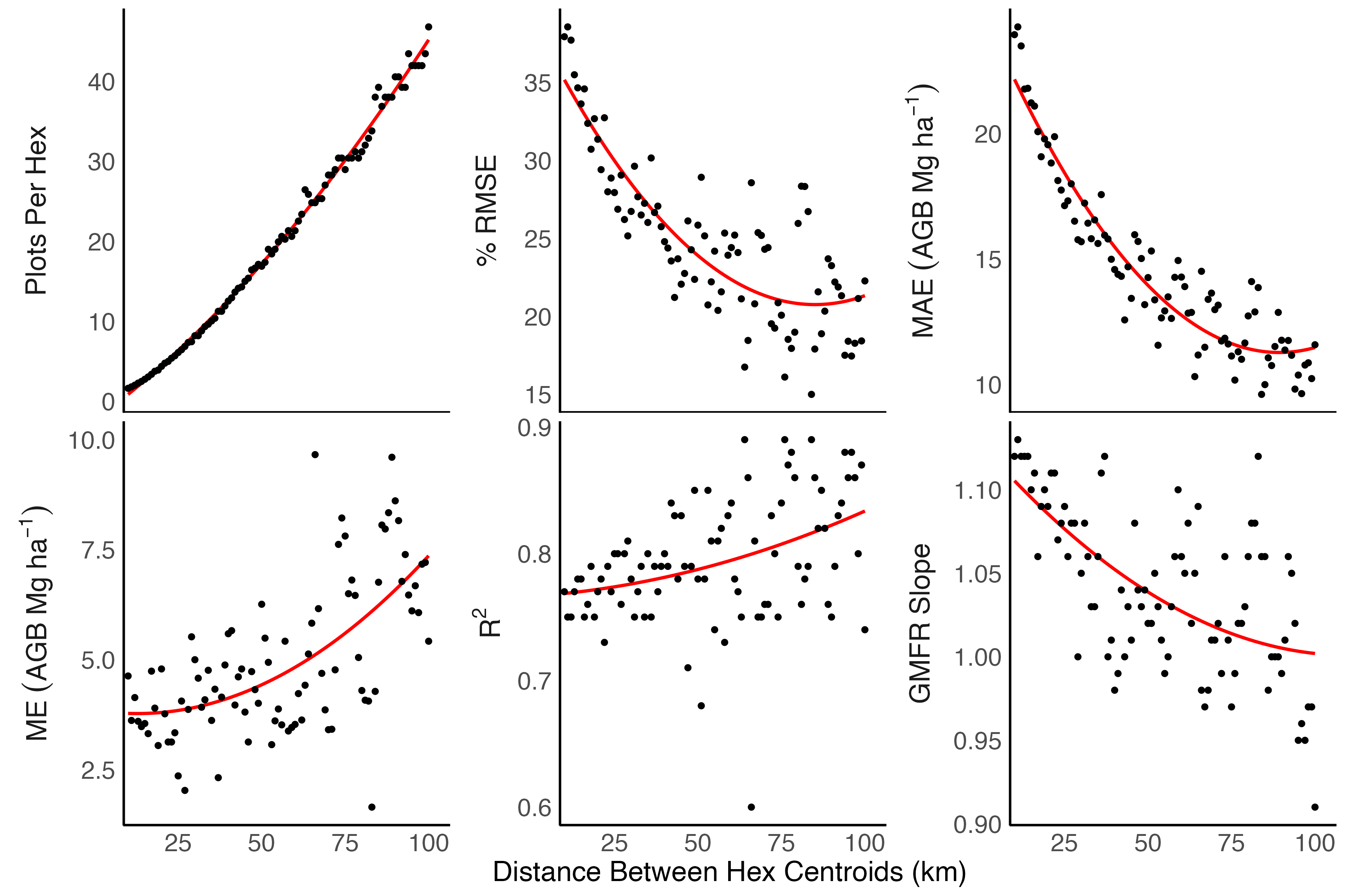
Figure 6: Summary assessment metrics (as defined in Section 2.5) comparing mapped predictions to FIA estimates as a function of aggregation unit size (described by distances between hexagon centroids). Red trend lines produced using quadratic regression.

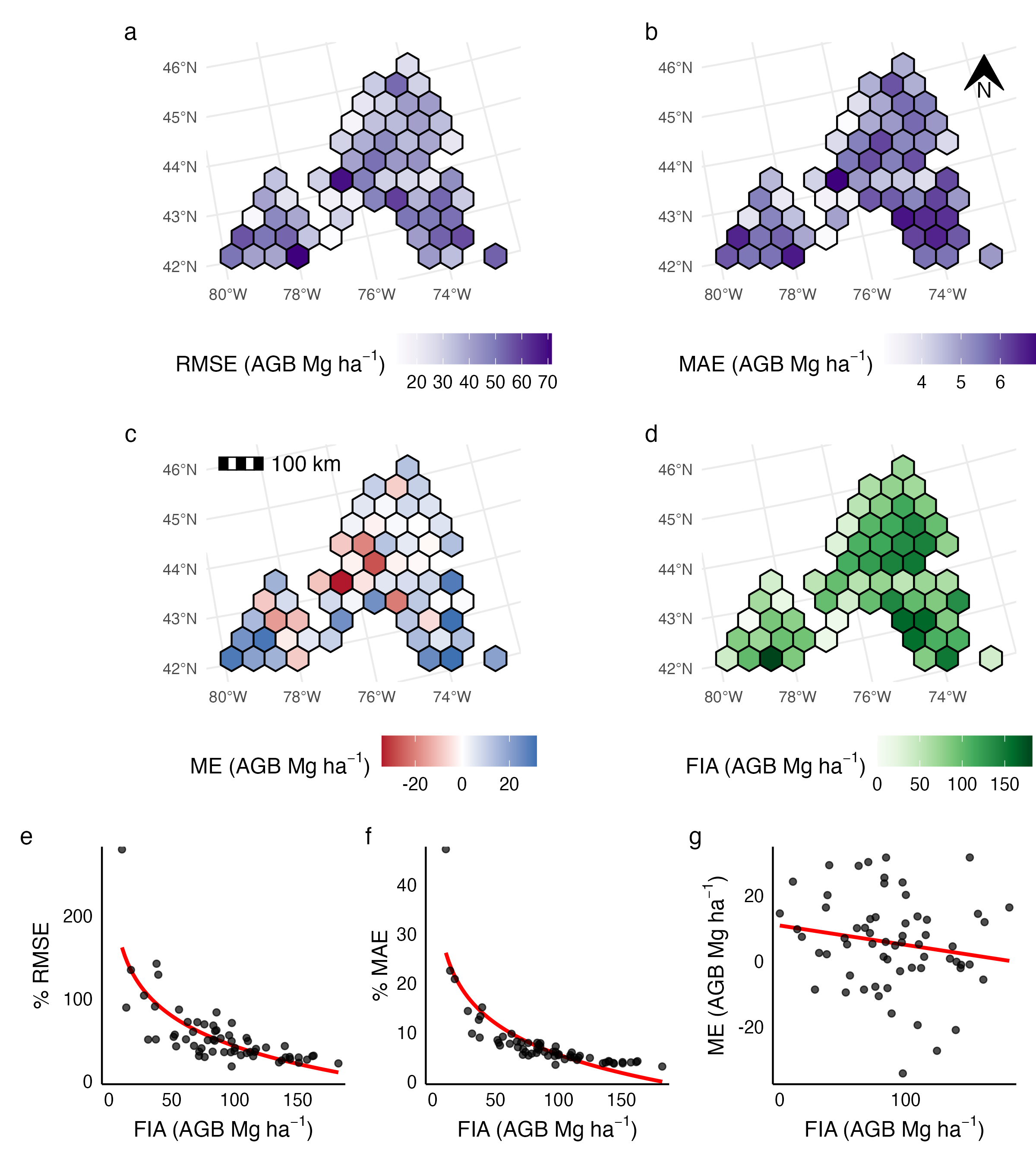
Figure 7: Plot-to-pixel residuals summarized at units spaced 50 km apart. Hexagons with only one reference plot were removed. a) RMSE Mg ha^-1 b) MAE Mg ha^-1 c) ME Mg ha^-1 d) Mean FIA AGB value Mg ha^-1 e) Hex-level % RMSE as a function of mean reference value f) Hex-level % MAE as a function of mean reference value. g) Hex-level ME as a function of mean reference value within each hexagon. 1 observation excluded from e and f where 0 FIA AGB makes % RMSE impossible to compute. Trend lines in e and f produced using logarithmic regression. Trend line in g produced using least-squares regression. RMSE, MAE, and ME as defined in Section 2.5.

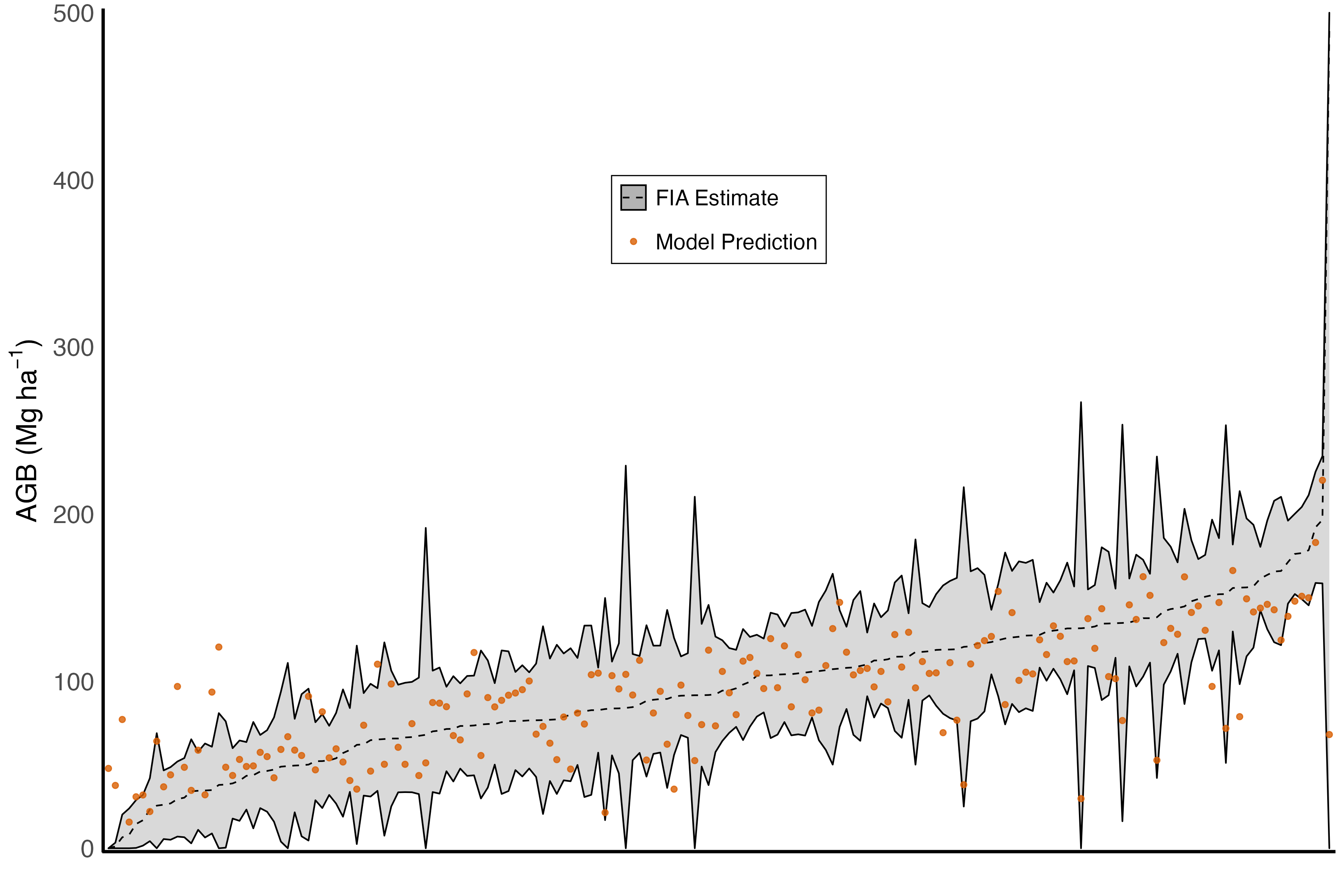
Figure 8: Comparison of mapped predicted AGB to Menlove and Healey (2020) estimates (dashed line) and associated 95% confidence interval (gray shaded region) within 64,000-ha aggregation hexagons. FIA estimates of AGB are scaled by the proportion of forest cover indicated by LCMAP 2016 Tree cover, Wetland, Croplands, and Grass/Shrub classified pixels. Hexagons with mapped areas $\leq$ 10% of their total area were excluded from this analysis. Observations are sorted by increasing FIA estimates along the x-axis.

Table 6: Map agreement at the plot to pixel scale, grouped by LCMAP classification. n = number of plots; RMSE, MAE, ME in Mg ha^-1. All accuracy metrics as defined in Section 2.5. Standard errors in parentheses, with a minimum of 0.01 for display.

LCMAP	n	% RMSE	RMSE	MAE	ME	R2
Tree Cover	797	36.35	45.85 (2.56)	34.42 (1.07)	3.83 (1.62)	0.55 (0.01)
Cropland	303	229.82	18.90 (2.40)	10.32 (0.91)	6.67 (1.02)	0.40 (0.03)
Wetland	91	62.48	51.36 (30.77)	35.56 (3.91)	-1.13 (5.41)	0.55 (0.01)
Grass/Shrub	26	119.65	23.71 (17.01)	16.03 (3.49)	14.64 (3.73)	0.50 (1.24)

4 Discussion

In this study we attempted to use a patchwork of 17 discrete LiDAR coverages for broad-scale, fine-resolution forest aboveground biomass (AGB) mapping across New York State (NYS), USA. Faced with a limited sample of temporally aligned field inventory data, we leveraged repeated inventories to boost the model training sample, and used a machine learning ensemble model to produce accurate predictions. We addressed concerns of sensor and mission discrepancies among component LiDAR coverages by investigating spatial patterns of prediction error, and by using an AOA mask to both show predictor uniformity across coverages, as well as to mask predictions based on anomalous data. Our results demonstrated that our maps accurately characterized the spatial patterns of AGB across the state, and showed that our predictions have strong agreement with FIA estimates across a range of aggregation scales.

4.1 Growth-Adjusted Field Plots

Our approach to solve the common lack of temporally coincident LiDAR and field data was parsimonious and effectively tripled the sample size while achieving accurate modeling results. We did this by leveraging the existing inventory data, without additional field campaigns, remotely sensed data, or growth and yield models. However, a potential limitation to this approach is the requirement of regular historical inventories so that bracketing inventory years can be identified for LiDAR acquisitions. Additionally, the maximum temporal distance between growth-adjusted AGB values and the nearest measured AGB values in our dataset was 10 years; growth-adjustment following our approach may not be reliable for longer temporal lags.

4.2 Pooled Modeling

Despite our efforts to boost the amount of training information available to models via growth adjustment, we were left with a non-uniform spatial arrangement of FIA plots across the GPO-LiDAR area. Several coverages contained fewer than 20 plots in the model dataset (Table 1), requiring a pooled modeling approach. Pooling information from all component LiDAR coverages allowed our model to borrow information from coverages with more training data to build relationships between our predictors and AGB that were then applied to coverages with less training data.

We relied on the computed AOA surface to enforce predictor space similarity with the training data, thus ensuring that our model did not predict into unknown predictor space, even in coverages with limited FIA plots. Moreover, the AOA surface provided evidence of predictor-space uniformity across all 17 component LiDAR coverages, indicating that each of the component coverages was well represented in the model training dataset (Meyer and Pebesma 2021). It stands to reason, however, that the NYC coverage contained the lowest proportion of AOA, since there were only two model plots available in this coverage (Table 1). Generally, pixels falling outside the AOA surface appeared to be the result of problems with LiDAR collection or data processing abnormalities, with some visible outliers that could not be attributed to any known ecological phenomena. We found the AOA mapping especially valuable in utilizing publicly available LiDAR coverages off the shelf with limited knowledge of, or responsibility for, their provenance.

4.3 Forest Definition Disparities

A forest can be defined in many ways depending on goals, perspectives, and operational concerns, and aligning the various definitions to make comparisons or derive relationships is neither a trivial nor a unique challenge (Chazdon et al. 2016; Riemann et al. 2010; Huang et al. 2019). FIA’s strict forest definition that is in part based on field observations of land-use, which is traditionally difficult to classify with remotely sensed data (Fritz et al. 2017), was difficult to harmonize with LiDAR. Since FIA does not provide a forest/nonforest map, and FIA’s definition of forest can exclude significant AGB stocks in areas containing tree cover (Johnson et al. 2015, 2014), we relied on LCMAP’s classifications of vegetated cover types to mask our prediction surfaces. Our AGB maps thus reflect a more inclusive definition of forest than FIA, incorporating AGB stocks across a broader range of conditions and land-uses. Despite these definitional differences, there was overlap between FIA forest and our LCMAP-derived definition, as evidenced by the non-zero FIA AGB averages for model dataset plots grouped within each of the four vegetated LCMAP classes (Table 4). Further, we were able to separate true zeros from structural zeros in FIA nonforest conditions using a 1 m LiDAR max-height threshold (Table 2), giving our model information to make predictions in areas with little to no canopy cover.

Although most of our mapped AGB was contained within pixels classified as tree cover, a significant minority was contained within pixels classified as Cropland and Grass/Shrub (Table 4). As the total area of agricultural lands has been declining in NYS (USDA National Agricultural Statistics Service 2019), we expect that many of these predictions represented early successional forests, or patches of ‘young and stunted trees’ in open fields (Yang et al. 2018), both transitional states which are challenges for LCMAP’s classification algorithm (Mahoney, Johnson, and Beier 2022; Brown et al. 2020). In summary, the landscape-level context in NYS, and LCMAP’s algorithmic challenges provided support to generate predictions for all LCMAP vegetated classes.

4.4 Model Performance and Map Agreement Assessment

Our prediction accuracy against the 20% testing partition of our model dataset was favorably comparable to previous LiDAR-AGB mapping studies (Huang et al. 2019; Nilsson et al. 2017; Ayrey et al. 2021; Hauglin et al. 2021). Using a set of FIA-developed methods (Riemann et al. 2010; Menlove and Healey 2020) we further demonstrated an overall strong agreement between our map-based estimates and FIA-derived estimates.

It is unsurprising that assessment metrics generally improved as the scales of aggregation increased, given that the plot-to-pixel scale can be considered the most rigorous, with the largest variance in both the pixel and plot AGB distributions, as well as the most potential for spatial misalignment between 30 m pixel predictions and FIA plot measurements to influence agreement metrics (McRoberts et al. 2018). When mapped residuals were summarized within units spaced 50 km apart, larger magnitudes of prediction error (RMSE, ME) emerged, but region or coverage specific patterns were not evident (Figure 7). Rather, we observed ME to be mostly positive across the GPO-LiDAR area, and to be weakly related to the underlying distribution of FIA reference data. We can also infer that large RMSE values were a reflection of extreme individual outliers as they were often paired with reasonable MAE values.

Our choice to maintain FIA’s probability sample in order to leverage unbiased estimators of map agreement metrics came with some drawbacks. Namely, we had to accept temporal lags of +/- 2 years between LiDAR acquisitions and field inventories, and we had to include structural zeros in our assessment dataset where FIA did not record tree measurements in non-forest conditions. It is likely that the former inflated our estimates of error due to growth or disturbances occurring at plots between the time of inventory and the time of LiDAR acquisition, though we have no means to quantitatively confirm this possibility. We can say with more certainty that the structural zeros introduced by non-forest plots had a large impact on our map agreement assessment as evidenced by the stack of non-zero predictions along the x-axis in plot to pixel comparisons (Figure 5) and the large positive ME for plots classified as Grass/Shrub and Cropland (Table 6). Given the large non-zero biomass predictions produced at these plots, it is not unreasonable to assume they contain trees unmeasured by FIA that would be captured by LiDAR height metrics. These structural zeros are likely the driving force behind the positive average prediction error (ME) found in our assessments, and may be the cause for the slight increase in Moran’s I values computed with the assessment dataset relative to those computed with the model dataset (Supplementary Materials S6).

Nearly all of our assessments, including performance against the testing partition of the model data (Figure 3), the Riemann analysis (Figure 5), agreement with the Menlove and Healey FIA estimates (Figure 8), and the weak relationship between ME and average FIA AGB estimate (Figure 7 g) reinforced our model’s tendency towards lower accuracy at the extremes of the FIA reference dataset. These discrepancies can likely be attributed to the model structure and training approach, the aforementioned structural zeros in our map assessment dataset, as well as the saturation problem inherent in LiDAR-AGB modeling (St-Onge, Hu, and Vega 2008) where models fail to predict the largest AGB values in the data set. In general, with the extremes of the response distribution occurring less often, most models will be more accurate making predictions near the mean.

We also recognize the presence of uncertainty in the AGB reference data due to allometric, measurement, and locational errors, as well as our growth adjustment procedure used to boost the size of the model dataset, though quantifying the magnitude of this uncertainty was outside the scope of this paper. Duncanson et al. (2017) indicated that different choices in allometric models used to predict AGB from tree diameter and height measurements can result in large variation (up to 20%) of plot-level AGB estimates. An improvement would be to embed measurement errors, as well as allometric and growth adjustment uncertainty in a quantification of model precision or uncertainty at the pixel level (CEOS 2021). Such information could help to develop variance estimates for any aggregation of pixel predictions that could be used in estimating AGB in areas that lack field inventories (Dettmann et al. 2022; CEOS 2021).

4.5 Map Applications

Our rigorously evaluated map products have a range of applications where knowledge of the spatial patterns of forest biomass (and by extension, forest carbon pools) is needed for monitoring, reporting, and verification efforts alongside policy or regulatory decision support. These uses include the identification of forested areas for future monitoring, protection, or management, and for providing AGB as a predictor in subsequent ecological models. Our AGB maps can also be leveraged as diverse training data for models driven by spaceborne remote sensing platforms with more contiguous spatial and temporal coverage than LiDAR patchworks, providing the basis for landscape-scale carbon accounting (Hudak et al. 2020; CEOS 2021).

5 Conclusion

Accurate AGB predictions at fine resolutions can provide landowners and decision makers with valuable information on landscape patterns needed to implement forest-based climate solutions, including reforestation opportunities, avoided deforestation, and improved management for carbon storage and sequestration. We implemented a model-based approach leveraging extensive field inventory data (FIA) and publicly available LiDAR coverages to develop AGB maps across NYS, where forests are expected to contribute substantially as carbon sinks towards achieving a net-zero carbon economy by 2050. Although LiDAR point clouds provide detailed information on forest structure that can yield superior models of forest biomass, their limited coverage in both spatial and temporal domains produces patchworks of disparate datasets over broad scales. Our modeling approach, and the comprehensive set of assessments demonstrated here, addressed several of the common challenges inherent in using LiDAR patchworks for AGB mapping, including a lack of temporally matching reference data and data discrepancies among component LiDAR coverages. Our results show that our approach and the resulting map products provide accurate AGB information at scales relevant to forest and climate stewardship in NYS.

6 Acknowledgements

We would like to thank the USDA FIA program for their data sharing and cooperation, the NYS GPO for compiling LiDAR data and sharing tax-parcel data, and the NYS Department of Environmental Conservation, Office of Climate Change, for funding support.

References

reAnderson, Ryan S., and Paul V. Bolstad. 2013. “Estimating Aboveground Biomass and Average Annual Wood Biomass Increment with Airborne Leaf-on and Leaf-off LiDAR in Great Lakes Forest Types.” Northern Journal of Applied Forestry 30 (1): 16–22. https://doi.org/10.5849/njaf.12-015.

preAyrey, Elias, Daniel J. Hayes, John B. Kilbride, Shawn Fraver, John A. Kershaw, Bruce D. Cook, and Aaron R. Weiskittel. 2021. “Synthesizing Disparate LiDAR and Satellite Datasets Through Deep Learning to Generate Wall-to-Wall Regional Inventories for the Complex, Mixed-Species Forests of the Eastern United States.” Remote Sensing 13 (24). https://doi.org/10.3390/rs13245113.

preBechtold, William A, and Paul L Patterson. 2005. The Enhanced Forest Inventory and Analysis Program–National Sampling Design and Estimation Procedures. Vol. 80. USDA Forest Service, Southern Research Station. https://doi.org/10.2737/SRS-GTR-80.

preBivand, Roger S., Edzer Pebesma, and Virgilio Gomez-Rubio. 2013. Applied Spatial Data Analysis with R, Second Edition. Springer, NY. https://doi.org/10.1007/978-0-387-78171-6.

preBreiman, Leo. 2001a. “Random Forests.” Machine Learning 45 (1): 5–32. https://doi.org/10.1023/A:1010933404324.

pre———. 2001b. “Statistical Modeling: The Two Cultures.” Statistical Science 16 (3): 199–231. https://doi.org/10.1214/ss/1009213726.

preBrown, Jesslyn F., Heather J. Tollerud, Christopher P. Barber, Qiang Zhou, John L. Dwyer, James E. Vogelmann, Thomas R. Loveland, et al. 2020. “Lessons learned implementing an operational continuous United States national land change monitoring capability: The Land Change Monitoring, Assessment, and Projection (LCMAP) approach.” Remote Sensing of Environment 238: 111356. https://doi.org/10.1016/j.rse.2019.111356.

preBuendia, E, K Tanabe, A Kranjc, J Baasansuren, M Fukuda, S Ngarize, A Osako, Y Pyrozhenko, P Shermanau, and S Federici. 2019. “Refinement to the 2006 IPCC Guidelines for National Greenhouse Gas Inventories.” IPCC: Geneva, Switzerland 5: 194.

preCEOS. 2021. “Aboveground Woody Biomass Product Validation Good Practices Protocol.” https://doi.org/10.5067/DOC/CEOSWGCV/LPV/AGB.001.

preChazdon, Robin L, Pedro HS Brancalion, Lars Laestadius, Aoife Bennett-Curry, Kathleen Buckingham, Chetan Kumar, Julian Moll-Rocek, Ima Célia Guimarães Vieira, and Sarah Jane Wilson. 2016. “When Is a Forest a Forest? Forest Concepts and Definitions in the Era of Forest and Landscape Restoration.” Ambio 45 (5): 538–50. https://doi.org/10.1007/s13280-016-0772-y.

preChen, Qi, and Ronald McRoberts. 2016. “Statewide Mapping and Estimation of Vegetation Aboveground Biomass Using Airborne Lidar.” In 2016 IEEE International Geoscience and Remote Sensing Symposium (IGARSS). IEEE. https://doi.org/10.1109/igarss.2016.7730157.

preCortes, Corinna, and Vladimir Vapnik. 1995. “Support-Vector Networks.” Machine Learning 20 (3): 273–97. https://doi.org/10.1007/bf00994018.

preDaniel Baston. 2021. Exactextractr: Fast Extraction from Raster Datasets Using Polygons. https://CRAN.R-project.org/package=exactextractr.

preDettmann, Garret T, Philip J Radtke, John W Coulston, P Corey Green, Barry T Wilson, and Gretchen G Moisen. 2022. “Review and Synthesis of Estimation Strategies to Meet Small Area Needs in Forest Inventory.” https://doi.org/10.3389/ffgc.2022.813569 .

preDuncanson, Laura, Wenli Huang, Kristofer Johnson, Anu Swatantran, Ronald E McRoberts, and Ralph Dubayah. 2017. “Implications of Allometric Model Selection for County-Level Biomass Mapping.” Carbon Balance and Management 12 (1): 1–11. https://doi.org/10.1186/s13021-017-0086-9.

preEfron, Bradley. 2020. “Prediction, Estimation, and Attribution.” Journal of the American Statistical Association 115 (530): 636–55. https://doi.org/10.1080/01621459.2020.1762613.

preFassnacht, F. E., F. Hartig, H. Latifi, C. Berger, J. Hernández, P. Corvalán, and B. Koch. 2014. “Importance of Sample Size, Data Type and Prediction Method for Remote Sensing-Based Estimations of Aboveground Forest Biomass.” Remote Sensing of Environment 154: 102–14. https://doi.org/10.1016/j.rse.2014.07.028.

preFriedman, Jerome H. 2002. “Stochastic Gradient Boosting.” Computational Statistics and Data Analysis 38 (4): 367–78. https://doi.org/10.1016/S0167-9473(01)00065-2.

preFritz, Steffen, Linda See, Christoph Perger, Ian McCallum, Christian Schill, Dmitry Schepaschenko, Martina Duerauer, et al. 2017. “A Global Dataset of Crowdsourced Land Cover and Land Use Reference Data.” Scientific Data 4 (1). https://doi.org/10.1038/sdata.2017.75.

preGobakken, Terje, and Erik Næsset. 2008. “Assessing Effects of Laser Point Density, Ground Sampling Intensity, and Field Sample Plot Size on Biophysical Stand Properties Derived from Airborne Laser Scanner Data.” Canadian Journal of Forest Research 38 (5): 1095–1109. https://doi.org/10.1139/X07-219.

preGonçalves, Fabio, Robert Treuhaft, Beverly Law, André Almeida, Wayne Walker, Alessandro Baccini, João dos Santos, and Paulo Graça. 2017. “Estimating Aboveground Biomass in Tropical Forests: Field Methods and Error Analysis for the Calibration of Remote Sensing Observations.” Remote Sensing 9 (1): 47. https://doi.org/10.3390/rs9010047.

preGray, Andrew N, Thomas J Brandeis, John D Shaw, William H McWilliams, and Patrick Miles. 2012. “Forest Inventory and Analysis Database of the United States of America (FIA).” Biodiversity and Ecology 4: 225–31. https://doi.org/10.7809/b-e.00079.

preHauglin, Marius, Johannes Rahlf, Johannes Schumacher, Rasmus Astrup, and Johannes Breidenbach. 2021. “Large Scale Mapping of Forest Attributes Using Heterogeneous Sets of Airborne Laser Scanning and National Forest Inventory Data.” Forest Ecosystems 8 (1). https://doi.org/10.1186/s40663-021-00338-4.

preHawbaker, Todd J., Terje Gobakken, Adrian Lesak, Eric Trømborg, Kirk Contrucci, and Volker Radeloff. 2010. “Light Detection and Ranging-Based Measures of Mixed Hardwood Forest Structure.” Forest Science 56 (3): 313–26. https://doi.org/10.1093/forestscience/56.3.313.

preHijmans, Robert J. 2021. Raster: Geographic Data Analysis and Modeling. https://CRAN.R-project.org/package=raster.

pre———. 2022. Terra: Spatial Data Analysis. https://CRAN.R-project.org/package=terra.

preHoppus, Michael, and Andrew Lister. 2005. “The Status of Accurately Locating Forest Inventory and Analysis Plots Using the Global Positioning System.” In Proceedings of the Seventh Annual Forest Inventory and Analysis Symposium. https://www.nrs.fs.fed.us/pubs/7040.

preHoughton, R. A., J. I. House, J. Pongratz, G. R. van der Werf, R. S. DeFries, M. C. Hansen, C. Le Quéré, and N. Ramankutty. 2012. “Carbon Emissions from Land Use and Land-Cover Change.” Biogeosciences 9 (12): 5125–42. https://doi.org/10.5194/bg-9-5125-2012.

preHoughton, RA. 2005. “Aboveground Forest Biomass and the Global Carbon Balance.” Global Change Biology 11 (6): 945–58.

preHuang, Wenli, Katelyn Dolan, Anu Swatantran, Kristofer Johnson, Hao Tang, Jarlath O’Neil-Dunne, Ralph Dubayah, and George Hurtt. 2019. “High-resolution mapping of aboveground biomass for forest carbon monitoring system in the Tri-State region of Maryland, Pennsylvania and Delaware, USA.” Environmental Research Letters 14 (9): 095002. https://doi.org/10.1088/1748-9326/ab2917.

preHudak, Andrew T, Patrick A Fekety, Van R Kane, Robert E Kennedy, Steven K Filippelli, Michael J Falkowski, Wade T Tinkham, et al. 2020. “A Carbon Monitoring System for Mapping Regional, Annual Aboveground Biomass Across the Northwestern USA.” Environmental Research Letters 15 (9): 095003. https://doi.org/10.1088/1748-9326/ab93f9.

preHurtt, G, M Zhao, R Sahajpal, A Armstrong, R Birdsey, E Campbell, K Dolan, et al. 2019. “Beyond MRV: high-resolution forest carbon modeling for climate mitigation planning over Maryland, USA.” Environmental Research Letters 14 (4): 045013. https://doi.org/10.1088/1748-9326/ab0bbe.

preJean-Romain, Roussel, David Auty, Nicholas C. Coops, Piotr Tompalski, Tristan R. H. Goodbody, Andrew Sánchez Meador, Jean-François Bourdon, Florian de Boissieu, and Alexis Achim. 2020. “lidR: An R package for analysis of Airborne Laser Scanning (ALS) data.” Remote Sensing of Environment 251: 112061. https://doi.org/10.1016/j.rse.2020.112061.

preJohnson, Kristofer D, Richard Birdsey, Jason Cole, Anu Swatantran, Jarlath O’Neil-Dunne, Ralph Dubayah, and Andrew Lister. 2015. “Integrating LIDAR and Forest Inventories to Fill the Trees Outside Forests Data Gap.” Environmental Monitoring and Assessment 187 (10): 1–8. https://doi.org/10.1007/s10661-015-4839-1.

preJohnson, Kristofer D, Richard Birdsey, Andrew O Finley, Anu Swantaran, Ralph Dubayah, Craig Wayson, and Rachel Riemann. 2014. “Integrating Forest Inventory and Analysis Data into a LIDAR-Based Carbon Monitoring System.” Carbon Balance and Management 9 (1). https://doi.org/10.1186/1750-0680-9-3.

preKaratzoglou, Alexandros, Alexandros Smola, Kurt Hornik, and Achim Zeileis. 2004. “kernlab - An S4 Package for Kernel Methods in R.” Journal of Statistical Software, Articles 11 (9): 1–20. https://doi.org/10.18637/jss.v011.i09.

preKe, Guolin, Qi Meng, Thomas Finley, Taifeng Wang, Wei Chen, Weidong Ma, Qiwei Ye, and Tie-Yan Liu. 2017. “LightGBM: A Highly Efficient Gradient Boosting Decision Tree.” In Advances in Neural Information Processing Systems, edited by I. Guyon, U. V. Luxburg, S. Bengio, H. Wallach, R. Fergus, S. Vishwanathan, and R. Garnett. Vol. 30. Curran Associates, Inc. https://proceedings.neurips.cc/paper/2017/file/6449f44a102fde848669bdd9eb6b76fa-Paper.pdf.

preKe, Guolin, Damien Soukhavong, James Lamb, Qi Meng, Thomas Finley, Taifeng Wang, Wei Chen, Weidong Ma, Qiwei Ye, and Tie-Yan Liu. 2021. Lightgbm: Light Gradient Boosting Machine. https://CRAN.R-project.org/package=lightgbm.

preKennedy, Robert E, Janet Ohmann, Matt Gregory, Heather Roberts, Zhiqiang Yang, David M Bell, Van Kane, et al. 2018. “An Empirical, Integrated Forest Biomass Monitoring System.” Environmental Research Letters 13 (2): 025004. https://doi.org/10.1088/1748-9326/aa9d9e.

preL’Roe, Andrew W, and Shorna Broussard Allred. 2013. “Thriving or Surviving? Forester Responses to Private Forestland Parcelization in New York State.” Small-Scale Forestry 12 (3): 353–76. https://doi.org/10.1007/s11842-012-9216-0.

preLu, Dengsheng, Qi Chen, Guangxing Wang, Lijuan Liu, Guiying Li, and Emilio Moran. 2014. “A Survey of Remote Sensing-Based Aboveground Biomass Estimation Methods in Forest Ecosystems.” International Journal of Digital Earth 9 (1): 63–105. https://doi.org/10.1080/17538947.2014.990526.

preMahoney, Michael J, Lucas K Johnson, and Colin M Beier. 2022. “Classification and Mapping of Low-Statured ’Shrubland’ Cover Types in Post-Agricultural Landscapes of the US Northeast.” arXiv. https://doi.org/10.48550/ARXIV.2205.05047.

preMcRoberts, Ronald E. 2011. “Satellite Image-Based Maps: Scientific Inference or Pretty Pictures?” Remote Sensing of Environment 115 (2): 715–24. https://doi.org/10.1016/j.rse.2010.10.013.

preMcRoberts, Ronald E., Qi Chen, Brian F. Walters, and Daniel J. Kaisershot. 2018. “The Effects of Global Positioning System Receiver Accuracy on Airborne Laser Scanning-Assisted Estimates of Aboveground Biomass.” Remote Sensing of Environment 207: 42–49. https://doi.org/10.1016/j.rse.2017.09.036.

preMenlove, James, and Sean P. Healey. 2020. “A Comprehensive Forest Biomass Dataset for the USA Allows Customized Validation of Remotely Sensed Biomass Estimates.” Remote Sensing 12 (24): 4141. https://doi.org/10.3390/rs12244141.

preMeyer, Hanna, and Edzer Pebesma. 2021. “Predicting into unknown space? Estimating the area of applicability of spatial prediction models.” Methods in Ecology and Evolution 12 (9): 1620–33. https://doi.org/10.1111/2041-210x.13650.

preMoran, Patrick AP. 1950. “Notes on Continuous Stochastic Phenomena.” Biometrika 37 (1/2): 17–23. https://doi.org/10.2307/2332142.

preNilsson, Mats, Karin Nordkvist, Jonas Jonzén, Nils Lindgren, Peder Axensten, Jörgen Wallerman, Mikael Egberth, et al. 2017. “A nationwide forest attribute map of Sweden predicted using airborne laser scanning data and field data from the National Forest Inventory.” Remote Sensing of Environment 194: 447–54. https://doi.org/https://doi.org/10.1016/j.rse.2016.10.022.

prePebesma, Edzer. 2018. “Simple Features for R: Standardized Support for Spatial Vector Data.” The R Journal 10 (1): 439–46. https://doi.org/10.32614/RJ-2018-009.

prePengra, Bruce, Steve Stehman, Josephine A Horton, Daryn J Dockter, Todd A Schroeder, Zhiqiang Yang, Alex J Hernandez, et al. 2020. “LCMAP Reference Data Product 1984-2018 Land Cover, Land Use and Change Process Attributes (Ver. 1.2, November 2021).” https://doi.org/10.5066/P9ZWOXJ7.

prePflugmacher, Dirk, Warren B. Cohen, Robert E. Kennedy, and Zhiqiang Yang. 2014. “Using Landsat-derived disturbance and recovery history and lidar to map forest biomass dynamics.” Remote Sensing of Environment 151: 124–37. https://doi.org/10.1016/j.rse.2013.05.033.

preR Core Team. 2021. R: A Language and Environment for Statistical Computing. Vienna, Austria: R Foundation for Statistical Computing. https://www.R-project.org/.

preRiemann, Rachel, Barry Tyler Wilson, Andrew Lister, and Sarah Parks. 2010. “An effective assessment protocol for continuous geospatial datasets of forest characteristics using USFS Forest Inventory and Analysis (FIA) data.” Remote Sensing of Environment 114 (10): 2337–52. https://doi.org/10.1016/j.rse.2010.05.010.

preRoussel, Jean-Romain, and David Auty. 2020. Airborne LiDAR Data Manipulation and Visualization for Forestry Applications. https://cran.r-project.org/package=lidR.

preSkowronski, Nicholas S, and Andrew J Lister. 2012. “Utility of LiDAR for large area forest inventory applications.” In In: Morin, Randall s.; Liknes, Greg c., Comps. Moving from Status to Trends: Forest Inventory and Analysis (FIA) Symposium 2012; 2012 December 4-6; Baltimore, MD. Gen. Tech. Rep. NRS-p-105. Newtown Square, PA: US Department of Agriculture, Forest Service, Northern Research Station.[CD-ROM]: 410-413., 410–13. https://www.fs.usda.gov/treesearch/pubs/42792.

preStehman, Stephen V., and Giles M. Foody. 2019. “Key Issues in Rigorous Accuracy Assessment of Land Cover Products” 231 (September): 111199. https://doi.org/10.1016/j.rse.2019.05.018.

preSt-Onge, B., Y. Hu, and C. Vega. 2008. “Mapping the height and above-ground biomass of a mixed forest using lidar and stereo Ikonos images.” International Journal of Remote Sensing 29 (5): 1277–94. https://doi.org/10.1080/01431160701736505.

preThompson, Jonathan R., David R. Foster, Robert Scheller, and David Kittredge. 2011. “The influence of land use and climate change on forest biomass and composition in Massachusetts, USA.” Ecological Applications 21 (7): 2425–44. https://doi.org/10.1890/10-2383.1.

preUSDA National Agricultural Statistics Service. 2019. “2017 Census of Agriculture.” https://www.nass.usda.gov/Publications/AgCensus/2017/index.php.

preWhite, Joanne C., John T. T. R. Arnett, Michael A. Wulder, Piotr Tompalski, and Nicholas C. Coops. 2015. “Evaluating the Impact of Leaf-on and Leaf-Off Airborne Laser Scanning Data on the Estimation of Forest Inventory Attributes with the Area-Based Approach.” Canadian Journal of Forest Research 45 (11): 1498–1513. https://doi.org/10.1139/cjfr-2015-0192.

preWhite, Joanne C., Michael A. Wulder, Andrés Varhola, Mikko Vastaranta, Nicholas C. Coops, Bruce D. Cook, Doug Pitt, and Murray Woods. 2013. “A Best Practices Guide for Generating Forest Inventory Attributes from Airborne Laser Scanning Data Using an Area-Based Approach.” The Forestry Chronicle 89 (06): 722–23. https://doi.org/10.5558/tfc2013-132.

preWintle, B. A., M. A. McCarthy, C. T. Volinksy, and R. P. Kavanagh. 2003. “The Use of Bayesian Model Averaging to Better Represent Uncertainty in Ecological Models.” Conservation Biology 17 (6): 1579–90. https://doi.org/10.1111/j.1523-1739.2003.00614.x.

preWolpert, David H. 1992. “Stacked Generalization.” Neural Networks 5 (2): 241–59. https://doi.org/10.1016/S0893-6080(05)80023-1.

preWoodall, Christopher W, John W Coulston, Grant M Domke, Brian F Walters, David N Wear, James E Smith, Hans-Erik Andersen, et al. 2015. “The US Forest Carbon Accounting Framework: Stocks and Stock Change, 1990-2016.” Gen. Tech. Rep. NRS-154. Newtown Square, PA: US Department of Agriculture, Forest Service, Northern Research Station. 49 p. 154: 1–49. https://doi.org/10.2737/NRS-GTR-154.

preWright, Marvin N., and Andreas Ziegler. 2017. “Ranger: A Fast Implementation of Random Forests for High Dimensional Data in c++ and r.” Journal of Statistical Software, Articles 77 (1): 1–17. https://doi.org/10.18637/jss.v077.i01.

preWulder, Michael A., David P. Roy, Volker C. Radeloff, Thomas R. Loveland, Martha C. Anderson, David M. Johnson, Sean Healey, et al. 2022. “Fifty Years of Landsat Science and Impacts.” Remote Sensing of Environment 280: 113195. https://doi.org/10.1016/j.rse.2022.113195.

preYang, Limin, Suming Jin, Patrick Danielson, Collin Homer, Leila Gass, Stacie M. Bender, Adam Case, et al. 2018. “A new generation of the United States National Land Cover Database: Requirements, research priorities, design, and implementation strategies.” ISPRS Journal of Photogrammetry and Remote Sensing 146 (December): 108–23. https://doi.org/10.1016/j.isprsjprs.2018.09.006.

preZhu, Zhe, and Curtis E. Woodcock. 2014. “Continuous change detection and classification of land cover using all available Landsat data.” Remote Sensing of Environment 144: 152–71. https://doi.org/10.1016/j.rse.2014.01.011.

p