Learning-Augmented Streaming Codes are Approximately Optimal for Variable-Size Messages

Abstract

Real-time streaming communication requires a high quality-of-service despite contending with packet loss. Streaming codes are a class of codes best suited for this setting. A key challenge for streaming codes is that they operate in an “online” setting in which the amount of data to be transmitted varies over time and is not known in advance. Mitigating the adverse effects of variability requires spreading the data that arrives at a time slot over multiple future packets, and the optimal strategy for spreading depends on the arrival pattern. Algebraic coding techniques alone are therefore insufficient for designing rate-optimal codes. We combine algebraic coding techniques with a learning-augmented algorithm for spreading to design the first approximately rate-optimal streaming codes for a range of parameter regimes that are important for practical applications.

I Introduction

Real-time communication arises in many popular applications, including VoIP, online gaming, and videoconferencing. These applications involve a sender transmitting packets of information to a receiver over a lossy channel. The receiver must decode the data within a strict playback deadline. In many scenarios, one cannot retransmit the lost packets because doing so requires an extra round trip time and can thus exceed the maximum tolerable latency [2]. Instead, one can use erasure coding to recover lost packets.

While erasure coding has been well studied, real-time communication has several unique aspects that require a new “streaming model,” as was introduced by Martinian and Sundberg [3]. During each time slot, $i$, a “message packet,” denoted as $S[i]$, of size $k$ arrives at a sender. The sender then transmits a “channel packet,” denoted as $X[i]$, of size $n$ to a receiver over a burst-only loss channel. The sender must recover $S[i]$ by time slot $(i+\tau)$. An overview of the model is presented in Figure 1, with the sender, channel, and receiver appearing in blue. (The component “side information” is introduced later.) Coding schemes that recover lost symbols from each message packet $\tau$ time slots later have significantly higher rates than alternatives, such as interleaved maximal distance separable codes, that recover all lost symbols together by $\tau$ time slots after the first message packet for which the symbols are lost [3].

Numerous works [4, 5, 6, 7, 8, 9, 10, 11, 12, 13, 14, 15, 16, 17, 18, 19, 20, 21, 22, 23, 24, 25] have employed tools from algebraic coding theory to design optimal streaming codes for various settings where the sizes of message packets and channel packets are fixed in advance. These regimes are suitable for applications that involve sending fixed quantities of data, such as VoIP when audio packets are sent uncompressed.

In contrast, many applications, such as videoconferencing, involve transmitting variable amounts of data. A new streaming model incorporating message packets of varying sizes was introduced in [26]. Two factors affect the optimal rate in this setting. First is the sequence of the sizes of all message packets of a transmission, called the “message packet size sequence.” Second is the maximum number of time slots the receiver can wait to decode each message packet under a lossless transmission, called “lossless delay” and denoted as $\tau_{L}$.

The optimal rate for “offline” schemes (which know the message packet size sequence) exceeds that of “online” schemes (which cannot access the sizes of message packets for future time slots) in all but two settings [27]. In one setting where $\tau_{L}$ has its maximum possible value, a technique for spreading the symbols of each message packet over several channel packets independently of all other message packets is rate optimal. The other setting, where $\tau_{L}$ has its minimum possible value (i.e., $0$), requires sending the symbols of each message packet in the corresponding channel packet. Therefore, information about the sizes of the future message packets does not help. Rate-optimal constructions, or even approximately rate-optimal constructions, are not known even for the offline setting for all remaining parameter regimes.

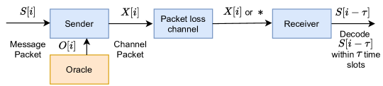
Figure 1: Overview of the model for streaming codes.

We consider the setting of $\tau_{L}=1$, which is important since it is the smallest value for which the symbols of a message packet can be spread over multiple channel packets. Spreading helps to significantly mitigate the adverse effect of variability of the sizes of message packets on the rate [26]. On the other hand, maintaining a small value of $\tau_{L}$ is crucial for latency-sensitive applications, as the delay of $\tau_{L}$ extra time slots may be incurred for decoding every message packet.

We first consider the offline setting and decompose the code design into two distinct challenges. First, how can we best spread message symbols over channel packets? Second, how can we send the minimum necessary number of parity symbols to ensure that each message packet is decoded in time, given any choice of how to spread message symbols? We use an integer program offline to determine how to optimally spread message symbols over channel packets. We then introduce a building block for constructing a rate-optimal streaming code for any given choice of how to spread message symbols over channel packets. One final challenge remains: how can we construct a rate-optimal online streaming code?

We address the problem by combining machine learning with tools from algebraic coding theory. We take a learning-based approach, relying on techniques similar to empirical risk minimization to convert the optimal offline solution into an approximately optimal online one that maximizes the expected rate. Our proposed method determines how to spread symbols online, and then the building block construction is applied.

Our methodology can be viewed as using a “learning-augmented algorithm”—a topic that has recently surged to prominence, tackling problems in other domains, such as caching [28], metric task systems [29], bloom filters [30], learned index structures [31], scheduling [32], etc. [33, 34, 35, 36, 37]. However, to the best of our knowledge, the powerful paradigm of learning-augmented algorithms has not been applied to design coding schemes until now.

Using machine learning models to perform encoding and/or decoding has received considerable attention in the recent past, including for channel coding [38, 39, 40, 41, 42, 43, 44, 45, 46], decoding with feedback [47, 48], approximate coded computation [49, 50, 51], MIMO [52, 53], etc. [54, 55, 56, 57, 58]. Most of these works use neural networks to handle encoding and or decoding in a black-box manner. In contrast, our work applies machine learning only to a small portion of the problem: to determine how to spread message symbols to address the uncertainty in the sizes of the future message packets. We then leverage tools from classical algebraic coding theory to solve the rest of the problem. This makes the learning part lightweight and interpretable and allows for theoretical guarantees on the rate.

II Model and background

We now present the system model used in this work, which is built on top of the model of streaming codes for variable-size messages [27, 26].

A transmission occurs over $(t+1)$ time slots for a non-negative integer $t$. During the $i$th time slot for $i\in\{0,\ldots,t\}$, the sender obtains a message packet, $S[i]\in\mathbb{F}^{k_{i}}$, where $\mathbb{F}$ is a finite field, and $k_{i}\in\{0,\ldots,m\}$ for a positive integer $m$. The sender also receives “side information,” $O[i]$, that captures the differences between the online and offline settings. In the offline setting, which assumes knowledge of the future, the side information is the sizes of the future message packets. In the online setting, the side information is independent $\mathcal{S}$ samples from the distribution of the sizes of future message packets for some positive integer $\mathcal{S}$. Let $D_{k_{0},\ldots,k_{i}}$ be the conditional distribution of $k_{i+1},\ldots,k_{t}$ given $k_{0},\ldots,k_{i}$. Then,

$$O[i]=\begin{cases}\left(k_{i+1},\ldots,k_{t}\right)&\text{if offline}\\ \big{\langle}\left(k_{i+1}^{(j)},\ldots,k_{t}^{(j)}\right)\sim D_{k_{0},\ldots,k_{i}}\mid j\in\{0,\ldots,\mathcal{S}-1\}\big{\rangle}&\text{if online}.\end{cases}$$ (1)

During the $i$th time slot, the sender transmits a channel packet, $X[i]\in\mathbb{F}^{n_{i}}$ to a receiver, where $n_{i}$ is a non-negative integer. The receiver obtains $Y[i]\in\{X[i],*\}$, which reflects packet reception or packet loss, respectively. When all channel packets are received, $S[i]$ must be decoded by the receiver by time slot $(i+\tau_{L})$ for a parameter $\tau_{L}\geq 0$. This requirement is called the “lossless-delay” constraint and represents the maximum tolerable latency for lossless transmission. Recall that our work considers $\tau_{L}=1$ (as discussed in Section I). In addition, $S[i]$ must be decoded by time slot $(i+\tau)$ when losses occur for a parameter $\tau\geq\tau_{L}$. This reflects the maximum acceptable latency in the worst case and is called the “worst-case-delay” constraint.

Our work uses the packet loss model from previous work [3, 4, 27]. Packets are lost in bursts of up to $b$ consecutive losses followed by at least $\tau$ successful receptions. Formally, for any $i\in\{0,\ldots,t-\tau-b+1\}$, if $\left(Y[i]=*\right)$ then $\forall j\in\{i+b,\ldots,i+b+\tau-1\}$ $\left(Y[j]=X[j]\right).$ To ensure that the worst-case-delay constraint is satisfiable, $\tau\geq b$. Furthermore, $b>0$ because coding is not needed otherwise. Finally, $\tau>b$, since $\tau\geq(\tau_{L}+b)$ [26] and $\tau_{L}=1$ in our work.

When the sizes of message packets and channel packets are fixed, the rate is simply the ratio of their sizes. However, a more nuanced notion of rate is needed due to the variability in the sizes of message packets and channel packets. The rate for a message packet size sequence $k_{0},\ldots,k_{t}$ is defined as

$$R_{t}=\frac{\sum_{i=0}^{t}k_{i}}{\sum_{i=0}^{t}n_{i}}.$$ (2)

For any integer $i$, $\{0,\ldots,i\}$ is denoted by $[i]$. For convenience of notation, $k_{i}=0$ for $i\in[2\tau-1]\cup\{t-2\tau+1,\ldots,t\},$ and $t$ is taken to be at least $4\tau$. This assumption is satisfied by adding zero padding, which does not affect the rate. As such, $S[0],\ldots,S[2\tau-1]$ are known to be of size zero, and $X[0],\ldots,X[2\tau-1]$ are empty. Encoding and decoding depends on the history of the transmission, which is summarized as follows.

Definition 1 (State)

For any $t,\tau,$ and $i\in\{2\tau,\ldots,t\}$, the state is denoted $\mathcal{X}_{i}=(k_{0},\ldots,k_{i},X[0],\ldots,X[i-1])$.

This section considers systematic codes for clarity, but the results also hold for general codes. To meet the lossless-delay constraint, the symbols of $S[i]$ must be sent by time slot $(i+\tau_{L})$ (i.e., in $X[i]$ and $X[i+1]$). The “policy” of a construction, as defined below, specifies how to spread the message symbols.

Definition 2 (Policy)

The policy of a construction for any $i\in[t]$ and state $\mathcal{X}_{i}$ is the number of symbols of $S[i]$ sent in channel packet $X[i]$. The policy is denoted as $\mathcal{F}_{i}\left(\mathcal{X}_{i}\right)$ (or $f_{i}$ for conciseness) and lies in $[k_{i}]$.

For any $i>0$, $X[i]$ comprises (a) the first $f_{i}$ symbols of $S[i]$, (b) the final $(k_{i-1}-f_{i-1})$ symbols of $S[i-1]$, and (c) $p_{i}$ parity symbols, denoted as $P[i]$. The encoding is given by $X[i]=$

$$Enc(\mathcal{X}_{i},S[i-\tau],\ldots,S[i-1],S_{0}[i],\ldots,S_{f_{i}-1}[i],O[i])$$ (3)

for $i\geq 2\tau$, and $X[i]$ is empty for $i<2\tau$. This section assumes that $X[i]$ is independent of the message symbols of $S[i]$ sent in $X[i+1]$ for clarity, although the results hold without this assumption. The receiver obtains $Y[i]\in\{X[i],*\}$ depending on whether channel packet $X[i]$ is received or dropped. Under lossless transmission, $S[i]$ is available in uncoded form. Otherwise, $S[i]$ is decoded as

$$Dec\left(\left\langle Y[j],k_{j},f_{j}\mid j\in[i+\tau]\right\rangle\right).$$ (4)

The following notation is used throughout our work. A vector $V$ has length $v$, comprises symbols $(V_{0},\ldots,V_{v-1})$, and is a row vector. For any $i\leq j\in[v-1]$, $V_{i}^{j}=(V_{i},\ldots,V_{j})$.

III A Building block construction

In this section, we present a rate-optimal construction, called the “$\left(\tau,b,t,\left\langle f_{i}\mid i\in[t]\right\rangle\right)-$Spread Code,” for any given policies, i.e., choice of how to spread the message symbols over channel packets. Specifically, for any given $\left\langle f_{i}\mid i\in[t]\right\rangle$, at least $f_{i}$ symbols of $S[i]$ will be sent in $X[i]$ under the construction for each $i\in[t]$.

The first $2\tau$ channel packets are empty. For each $i\in[t]\setminus[2\tau-1]$, $X[i]$ comprises (a) the first $f_{i}^{\prime}$ symbols of $S[i]$ for some $f_{i}^{\prime}\geq f_{i}$, (b) the final $(k_{i-1}-f_{i-1}^{\prime})$ symbols of $S[i-1]$, and (c) $p_{i}$ parity symbols called $P[i]$. Next, we define $f_{i}^{\prime}$, $p_{i}$, and $P[i]$ for any message packet size sequence, $k_{0},\ldots,k_{t}$.

Defining each $f_{i}^{\prime}$ and $p_{i}$. For time slots $i\in[2\tau-1]\cup\{t-2\tau+1,\ldots,t\}$, $f_{i}^{\prime}=k_{i}=0$. For time slots $i\in[3\tau-1]\cup\{t-\tau+1,\ldots,t\}$, $p_{i}=0$. For all $i=2\tau,\ldots,(t-2\tau)$, we define $p_{i+\tau}$ to be as small as possible while ensuring that $S[i]$ is decoded by time slot $(i+\tau)$ under any lossy transmission. Specifically, $p_{i+\tau}=$

$$\max_{j\in\{i-b+1,\ldots,i+1\}}\Big{(}0,\mathds{1}[j+b-1\geq i+1]\left(k_{i}-f_{i}\right)+\mathds{1}[j\leq i]f_{i}+\sum_{l=j}^{i}(k_{l-1}-f_{l-1}^{\prime})+\sum_{l=j}^{i-1}f_{l}^{\prime}-\sum_{l=j+b}^{i+\tau-1}p_{l}\Big{)},$$ (5)

as is illustrated in Figure LABEL:fig:codeParity. We then use $p_{i+\tau}$ to define

$$f_{i}^{\prime}=\max\left(f_{i},p_{i+\tau}\right).$$ (6)

Constructing parity symbols. The parity symbols are defined analogously to those of the construction from [27] (which builds on the construction from [5]). For $i\in\{2\tau,\ldots,t-\tau\}$, the message symbols sent in $X[i]$ are partitioned into (a) symbols of $S[i]$ that are recovered during time slot $(i+\tau)$ under a lossy transmission, and (b) symbols of $S[i-1]$ and $S[i]$ that are recovered by time slot $(i-1+\tau)$ under a lossy transmission. The two components are of sizes $u_{i}$ and $v_{i}$ and are denoted as $U[i]$ and $V[i]$, respectively. Thus, $X[i]=\left(U[i],V[i],P[i]\right)$, where

$$U[i] =S_{0}^{p_{i+\tau}-1}[i]$$ (7)

$$V[i] =\big{(}S_{p_{i+\tau}}^{k_{i}-f_{i}^{\prime}-1}[i],S_{f_{i-1}^{\prime}}^{k_{i-1}-1}[i-1]\big{)}$$ (8)

$$P[i] =U[i-\tau]+P^{(v)}[i].$$ (9)

Each symbol of $P^{(v)}[i]$ is a linear combination of the symbols of $\left(V[i-\tau],\ldots,V[i-1]\right)$, where the linear equations are chosen using a $(2m\tau)\times(2m\tau)$ Cauchy matrix, $A$, as follows. Let $W[i]$ be a length $2m\tau$ vector where positions $2m(j\bmod\tau),\ldots,\left(2m(j\bmod\tau)+2m-1\right)$ comprise $V[j]$ followed by $(2m-v_{j})$ $0$’s for $j\in\{i-\tau,\ldots,i-1\}$, as is illustrated in Figure 2.

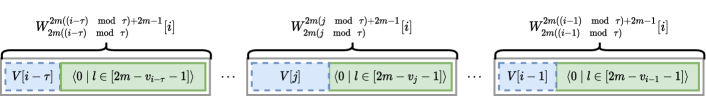
Figure 2: Defining $W[i]$ by placing the symbols of $V[i-\tau]$ in positions $2m(j\bmod\tau),\ldots,\left(2m(j\bmod\tau)+v_{j}-1\right)$ for $j\in\{i-\tau,\ldots,i-1\}$. The remaining positions are filled with $0$’s.

Finally, we define

$$P^{(v)}[i]=W[i]A_{(i)},$$ (10)

where $A_{(i)}$ is $A$ restricted to columns $2m(i\bmod\tau),\ldots,\left(2m(i\bmod\tau)+p_{i}-1\right)$. The $\left(\tau,b,t,\left\langle f_{i}\mid i\in[t]\right\rangle\right)-$Spread Code is shown recovering a burst in Figure LABEL:fig:spreading.

Decoding. For $i\in[t]$, $S[i]$ is decoded (a) from $X[i]$ and $X[i+1]$ under lossless conditions, and (b) by solving a system of linear equations corresponding to the symbols of $S[i-\tau],\ldots,S[i-1],Y[i],\ldots,Y[i+\tau]$ when losses occur.

Next, we show that the $\left(\tau,b,t,\left\langle f_{i}\mid i\in[t]\right\rangle\right)-$Spread Code meets the lossless-delay and worst-case-delay constraints.

Lemma 1

For any parameters $(\tau,b$), an arbitrary message packet size sequence $k_{0},\ldots,k_{t}$, and any policy $f_{i}$ for $i\in[t]$, the $\left(\tau,b,t,\left\langle f_{i}\mid i\in[t]\right\rangle\right)-$Spread Code satisfies the lossless-delay constraint and worst-case-delay constraint.

Proof:

For any $i\in[t-1]$, $S[i]=\left(S_{0}^{f_{i}^{\prime}-1}[i],S_{f_{i}^{\prime}}^{k_{i}-1}[i]\right)$, where $S_{0}^{f_{i}^{\prime}-1}[i]$ is sent in $X[i]$, and $S_{f_{i}^{\prime}}^{k_{i}-1}[i]$ is sent in $X[i+1]$. For $S[t]$, $k_{t}=0$ is known. Thus, the lossless-delay constraint is met.

Next, we show that the worst-case-delay is satisfied for any burst. Satisfaction is immediate if the burst starts after $(t-\tau-b+1)$, since $k_{t-\tau-b}=0,\ldots,k_{t}=0$ is known. Otherwise, suppose $X[i],\ldots,X[i+b-1]$ are lost for some $i\in[t-\tau-b+1]$. We assume that $i\geq 2\tau$, since $k_{0}=0,\ldots,k_{2\tau-1}=0$ is known, and no symbols are sent in $X[0],\ldots,X[2\tau-1]$. Each $P^{(v)}[i+b]=\left(P[i+b]-U[i+b-\tau]\right),\ldots,P^{(v)}[i+\tau-1]=\left(P[i+\tau-1]-U[i-1]\right)$ is known.

We show that enough parity symbols are received after the burst by time slot $(i+\tau-1)$ to recover $V[i],\ldots,V[i+b-1]$ as follows:

$$f_{i+b-1}+\sum_{j=i}^{i+b-1}\left(k_{j-1}-f_{j-1}^{\prime}\right)+\sum_{j=i}^{i+b-2}f_{j}^{\prime}\leq \sum_{j=i+b}^{i+b+\tau-1}p_{j}$$ (11)

$$\sum_{j=i}^{i+b-1}\left(k_{j-1}-f_{j-1}^{\prime}+f_{j}^{\prime}\right)\leq \sum_{j=i+b}^{i+b+\tau-1}p_{j}$$ (12)

$$\sum_{j=i}^{i+b-1}v_{j}+u_{j}\leq \sum_{j=i+b}^{i+b+\tau-1}p_{j}$$ (13)

$$\sum_{j=i}^{i+b-1}v_{j}\leq \sum_{j=i+b}^{i+\tau-1}p_{j},$$ (14)

where Eq. (11) follows from Eq. (5), Eq. (12) follows from (a) $f_{i+b-1}^{\prime}=f_{i+b-1}$, or (b) combining $f_{i+b-1}^{\prime}=p_{i+b-1+\tau}$ with Eq. (5) to show

$$\sum_{j=i}^{i+b-1}\left(k_{j-1}-f_{j-1}^{\prime}\right)+\sum_{j=i}^{i+b-2}f_{j}^{\prime}=k_{i-1}-f_{i-1}^{\prime}+\sum_{j=i}^{i+b-2}k_{j}\leq\sum_{j=i+b}^{i+b+\tau-2}p_{j},$$

Eq. (13) follows from Eqs. (7) and (8), and Eq. (14) follows from Eqs. (7) and  (9).

Next, we show that $P[i+b],\ldots,P[i+\tau-1]$ suffice to recover $V[i],\ldots,V[i+b-1]$ Recall that $P^{(v)}[j]=W[j]A_{(j)}$ for $j\in\{i+b,\ldots,i+\tau-1\}$, where $W[j]$ contains $V[l]$ in positions

$$I^{(i,j)}=\bigcup_{l\in\{i,\ldots,i+b-1\}}\{2m(l\bmod\tau),\ldots,\left(2m(l\bmod\tau)+v_{l}-1\right)\},$$

as defined in Eq. (10) and illustrated in Figure 2. Let $W^{\prime}[j]$ be the vector of length $2m\tau$ with (a) $0$’s in positions in $I^{(i,j)}$, (b) $W_{r}[j]$ for positions $r\in[2m\tau-1]\setminus I$. The receiver can compute $W^{\prime}[j]$ and use it to determine $P^{*}[j]=\left(P^{(v)}[j]-W^{\prime}[j]A_{(j)}\right)$. Let $l_{0}=i,\ldots,l_{b-1}=(i+b-1)$, and $r=\arg\min_{l\in\{i,\ldots,i+b-1\}}(l\bmod\tau)$. Let $l_{0}^{\prime}=(i+b),\ldots,l_{\tau-b-1}=(i+\tau-1)$, and $r^{\prime}=\arg\min_{l\in\{i+b,\ldots,i+\tau-1\}}(l\bmod\tau)$. Then

$$\begin{bmatrix}P^{*}[l_{r^{\prime}-(i+b)}^{\prime}]^{T}\\ \vdots\\ P^{*}[l_{\tau-b-1}^{\prime}]^{T}\\ P^{*}[l_{0}^{\prime}]^{T}\\ \vdots\\ P^{*}[l_{r^{\prime}-(i+b)-1}^{\prime}]^{T}\end{bmatrix}^{T}=\begin{bmatrix}V[l_{(r-i)}]^{T}\\ \vdots\\ V[l_{b-1}]^{T}\\ V[l_{0}]^{T}\\ \vdots\\ V[l_{(r-i)-1}]^{T}\end{bmatrix}^{T}A_{(i)}^{\prime},$$ (15)

where $T$ means transpose, and $A_{(i)}^{\prime}$ is a submatrix of a Cauchy matrix of dimensions $\left(\sum_{j=i}^{i+b-1}v_{j}\right)\times\left(\sum_{j=i+b}^{i+\tau-1}p_{j}\right)$. As such, $A_{(i)}^{\prime}$ is full rank, allowing the receiver to solve for $V[i],\ldots,V[i+b-1]$.

Finally, for $j=i,\ldots,(i+b-1)$, the receiver uses the symbols of $V[j],\ldots,V[j+\tau-1]$ to compute $P^{(v)}[j+\tau]$, yielding $U[j]=\left(P[j+\tau]-P^{(v)}[j+\tau]\right)$. As $S[j]$ is sent over $V[j],U[j],$ and $V[j+1]$, it is recovered by time slot $(j+\tau)$. ∎

Next, we provide a lower bound on the number of parity symbols sent by any streaming code that satisfies the lossless-delay and worst-case-delay constraints. The bound is illustrated in Figure LABEL:fig:systematicConstraints

Lemma 2

Consider any $\tau,t,b$, and any streaming code that satisfies the lossless-delay and worst-case-delay constraints. Suppose for $l\in[t]$, the construction sends $p^{\dagger}_{l}$ parity symbols and uses policy $f_{l}$. For any $i\in\{3\tau,\ldots,t\}$ and $j\in\{i-\tau-b+1,\ldots,i-\tau+1\}$, the number of parity symbols satisfies

$$-f_{j-1}-\mathds{1}[j+b-1=i-\tau]\big{(}k_{i-\tau}-f_{i-\tau}\big{)}+\sum_{l=j-1}^{i-\tau}k_{l}\leq\sum_{l=j+b}^{i}p^{\dagger}_{l}.$$ (16)

Proof:

Suppose $X[j],\ldots,X[j+b-1]$ are lost. Due to the worst-case-delay constraint, $S[j-1],\ldots,S[i-\tau]$ must be recovered by time slot $i$. Thus, $\sum_{l=j-1}^{i-\tau}k_{l}$ symbols need to be decoded. Because the message packets are independent, the symbols of $X[0],\ldots,X[j-2]$ contain no information about $S[j-1],\ldots,S[i-\tau]$. By definition of encoding (that is, Eq. (3)), $X[j-1]$ contains $f_{j-1}$ symbols of $S[j-1]$, no additional information about $S[j-1]$, and no information about $S[j],\ldots,S[i-\tau]$. When $(j+b-1)==(i-\tau)$, $X[i-\tau+1]$ is received, and its message symbols include $(k_{i-\tau}-f_{i-\tau})$ symbols of $S[i-\tau]$. The remaining message symbols of $X[j+b],\ldots,X[i]$ correspond to $S[i-\tau+1],\ldots,S[i]$ and cannot be used to recover $S[j-1],\ldots,X[i-\tau]$ (independence of message packets). Altogether,

$$-f_{j-1}-\mathds{1}[j+b-1=i-\tau]\big{(}k_{i-\tau}-f_{i-\tau}\big{)}+\sum_{l=j-1}^{i-\tau}k_{l}$$

symbols corresponding to $S[j-1],\ldots,S[i-\tau]$ need to be recovered by time slot $i$. These symbols can only be recovered using the parity symbols of $X[j+b],\ldots,X[i]$, of which there are

$$\sum_{l=j+b}^{i}p^{\dagger}_{l}.$$

The symbols of message packets are drawn uniformly at random from the underlying field. Thus, the total number of parity symbols must match the number of message symbols to be decoded. ∎

We show the rate of the $\left(\tau,b,t,\left\langle f_{i}\mid i\in[t]\right\rangle\right)-$Spread Code matches that of any streaming code with policy $f_{i}$ for $i\in[t]$.

Lemma 3

For any $\tau,t,b$, and message packet size sequence $k_{0},\ldots,k_{t}$, the $\left(\tau,b,t,\left\langle f_{i}\mid i\in[t]\right\rangle\right)-$Spread Code matches the rate of any streaming code with policy $f_{i}$ for $i\in[t]$ that satisfies the lossless-delay and worst-case-delay constraints.

Proof:

Under the $\left(\tau,b,t,\left\langle f_{i}\mid i\in[t]\right\rangle\right)-$Spread Code, $\sum_{l=0}^{t}(k_{l}+p_{l})$ symbols are sent. Consider any streaming code construction that satisfies the lossless-delay and worst-case-delay constraints, and for each $i\in[t]$, employs policy $f_{i}$ and sends $p^{\dagger}_{i}$ parity symbols. This streaming code construction sends $\sum_{l=0}^{t}\left(k_{l}+p^{\dagger}_{l}\right)$ symbols in total.

We show by induction on $i=0,\ldots,t$ that $\sum_{l=0}^{i}p_{l}\leq\sum_{l=0}^{i}p^{\dagger}_{l}$. The base case holds for $j<3\tau$ because $p_{0}=0,\ldots,p_{3\tau-1}=0$. For the inductive hypothesis, we note for all $j<i$ :

$$\sum_{l=0}^{j}p_{l}\leq\sum_{l=0}^{j}p^{\dagger}_{l}.$$ (17)

In the inductive step, consider $i=3\tau,\ldots,t-\tau$. By Eq. (17), the proof holds if $p_{i}\leq p^{\dagger}_{i}$. Otherwise, $p_{i}>p^{\dagger}_{i}\geq 0$. Due to Eq. (17), we only need to show for $j\leq i$ that $\sum_{l=j}^{i}p_{l}\leq\sum_{l=j}^{i}p^{\dagger}_{l}$.

Let ${i_{*}}=(i-\tau)$. By Eq. (5), there exists ${j_{*}}\in\{{i_{*}}-b+1,\ldots,{i_{*}}+1\}$ (specifically, taking ${j_{*}}$ as the value of $j$ used to define $p_{i}$) such that

$$\sum_{l={j_{*}}+b}^{i}p_{l} =$$ (18)

$$\sum_{l={j_{*}}+b}^{{i_{*}}+\tau}p_{l} =\mathds{1}[{j_{*}}+b-1\geq{i_{*}}+1]\left(k_{{i_{*}}}-f_{{i_{*}}}\right)+\mathds{1}[{j_{*}}\leq{i_{*}}]f_{{i_{*}}}+\sum_{l={j_{*}}}^{{i_{*}}}(k_{l-1}-f_{l-1}^{\prime})+\sum_{l={j_{*}}}^{{i_{*}}-1}f_{l}^{\prime}$$ (19)

$$=-\mathds{1}[{j_{*}}={i_{*}}+1]f_{{j_{*}}-1}-\mathds{1}[{j_{*}}>({i_{*}}+1)]f_{{j_{*}}-1}^{\prime}-\mathds{1}[{j_{*}}+b-1={i_{*}}]\left(k_{{i_{*}}}-f_{{i_{*}}}\right)+\sum_{l={j_{*}}-1}^{{i_{*}}}k_{l}$$ (20)

$$=-f_{{j_{*}}-1}^{\prime}-\mathds{1}[{j_{*}}+b-1={i_{*}}]\left(k_{{i_{*}}}-f_{{i_{*}}}\right)+\sum_{l={j_{*}}-1}^{{i_{*}}}k_{l}$$ (21)

$$=-f_{{j_{*}}-1}^{\prime}-\mathds{1}[{j_{*}}+b-1=i-\tau]\left(k_{i-\tau}-f_{i-\tau}\right)+\sum_{l={j_{*}}-1}^{i-\tau}k_{l}$$ (22)

$$\leq-f_{{j_{*}}-1}-\mathds{1}[{j_{*}}+b-1=i-\tau]\left(k_{i-\tau}-f_{i-\tau}\right)+\sum_{l={j_{*}}-1}^{i-\tau}k_{l}.$$ (23)

Eq. (19) follows from the fact that ${i_{*}}=(i-\tau)$ and Eq. (5). Eq. (20) follows from rearranging terms. Eq. (21) is immediate if ${j_{*}}>{i_{*}}$ and otherwise follows from $p_{{i_{*}}+\tau}\leq f_{{i_{*}}}$ (by ${j_{*}}>{i_{*}}$ and Eq. (5)) leading to $f_{{i_{*}}}^{\prime}=f_{{i_{*}}}$ (by Eq. (6)). Eq. (22) follows from substituting ${i_{*}}=(i-\tau)$. Eq. (23) follows from Eq. (6).

By Lemma 2,

$$\sum_{l={j_{*}}+b}^{i}p^{\dagger}_{l}\geq-f_{{j_{*}}-1}-\mathds{1}[{j_{*}}+b-1=i-\tau]\big{(}k_{i-\tau}-f_{i-\tau}\big{)}+\sum_{l={j_{*}}-1}^{i-\tau}k_{l}.$$ (24)

Combining Eqs. (18),  (23) and (24) leads to

$$\sum_{l={j_{*}}+b}^{i}p^{\dagger}_{l}\geq\sum_{l={j_{*}}+b}^{i}p_{l}.$$ (25)

Applying Eq. (17) (for $j={j_{*}}+b-1$) to Eq. (25) leads to

$$\sum_{l=0}^{{j_{*}}+b-1}p^{\dagger}_{l}+\sum_{l={j_{*}}+b-1}^{i}p^{\dagger}_{l}=\sum_{l=0}^{i}p^{\dagger}_{l}\geq\sum_{l=0}^{{j_{*}}+b-1}p_{l}+\sum_{l={j_{*}}+b-1}^{i}p_{l}=\sum_{l=0}^{i}p_{l},$$ (26)

proving the inductive step for $l\in\{3\tau,\ldots,t-\tau\}$. Recall that $p_{t-\tau+1}=0,\ldots,p_{t}=0$, leading to

$$\sum_{l=0}^{t}p^{\dagger}_{l}\geq\sum_{l=0}^{t-\tau}p^{\dagger}_{l}\geq\sum_{l=0}^{t-\tau}p_{l}=\sum_{l=0}^{t}p_{l}.$$

The $\left(\tau,b,t,\left\langle f_{i}\mid i\in[t]\right\rangle\right)-$Spread Code sends $\sum_{l=0}^{t}(k_{l}+p_{l})$ symbols, which is no more than the number sent under the alternative construction (i.e., $\sum_{l=0}^{t}(k_{l}+p^{\dagger}_{l})$). ∎

IV Offline-optimal streaming codes

In this section, we design the first rate-optimal offline construction for the setting of $\tau_{L}=1$. We build the construction with two steps for an arbitrary message packet size sequence, $k_{0},\ldots,k_{t}$. First, we design an integer program (IP) to use constraints to model satisfying the lossless-delay and Lemma 2. The IP determines the optimal policy for each time slot: $\left\langle f_{i}\mid i\in[t]\right\rangle$, as is illustrated in Figure 3.

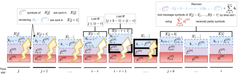
Figure 3: Modeling the transmission and constraints using the variables of the integer program. For any $i\in\{3\tau,\ldots,t-\tau\}$ and burst (lightning bolts) of length $b$ starting in $j\in\{i-\tau-b+1,\ldots,i-\tau+1\}$, $S[j-1],\ldots,S[i-\tau]$, are recovered by time slot $j$ under the relaxation of receiving the lost symbols of $S[i-\tau+1],\ldots,S[j+b-1]$ (boxes with thick black outline).

Second, we employ the $\left(\tau,b,t,\left\langle f_{i}\mid i\in[t]\right\rangle\right)-$Spread Code given the polices. The objective function of the integer program is to minimize the total number of parity symbols transmitted, which maximizes the rate.

Next, we introduce Algorithm 1 to determine an optimal policy, $f_{i}$, for each time slot $i\in[t]$ and then verify that the $\left(\tau,b,t,\left\langle f_{i}\mid i\in[t]\right\rangle\right)-$Spread Code is rate optimal.

Algorithm 1 Computes $\left\langle f_{i}\mid i\in[t]\right\rangle$ for which the $\left(\tau,b,t,\left\langle f_{i}\mid i\in[t]\right\rangle\right)-$Spread Code matches the offline-optimal-rate.

Input: $(\tau,b,t,k_{0},\ldots,k_{t})$

Minimize $\sum_{i=0}^{t}p^{(IP)}_{i}$ subject to

• $\forall i\in[t]$, $f^{(IP)}_{i}\geq 0,f^{(IP)}_{i}\leq k_{i},p^{(IP)}_{i}\geq 0$.

• $\forall i\in\{3\tau,\ldots,t-\tau\},j\in\{i-\tau-b+1,\ldots,i-\tau+1\}$,

$$-f^{(IP)}_{j-1}-\mathds{1}[j+b-1=i-\tau]\left(k_{i-\tau}-f^{(IP)}_{i-\tau}\right)+\sum_{l=j-1}^{i-\tau}k_{l}\leq\sum_{l=j+b}^{i}p^{(IP)}_{l}.$$

Output: $\left\langle f_{i}\mid i\in[t]\right\rangle$

Theorem 1

For any $(\tau,b,t)$ and message packet size sequence $k_{0},\ldots,k_{t}$, suppose Algorithm 1 outputs $\left\langle f_{i}\mid i\in[t]\right\rangle$. Then the $\left(\tau,b,t,\left\langle f_{i}\mid i\in[t]\right\rangle\right)-$Spread Code is rate optimal.

Proof:

Due to Lemma 3, the rate of the $\left(\tau,b,t,\left\langle f_{i}\mid i\in[t]\right\rangle\right)-$Spread Code is the same as a construction that for $i\in[t]$ employs the policy $f_{i}$ and sends $p^{(IP)}_{i}$ parity symbols in $X[i]$. We will show that no coding scheme can send fewer than $\sum_{i=0}^{t}p^{(IP)}_{i}$ parity symbols.

An arbitrary rate-optimal construction must satisfy the first constraint because for all $i\in[t]$ between $0$ and $k_{i}$ symbols of $S[i]$ are sent in $X[i]$ along with a non-negative number of parity symbols. The construction must satisfy the second constraint due to Lemma 2. Using each policy of this rate-optimal construction along with the number of parity symbols it sends is a valid solution to the integer program. Correctness follows from minimization. ∎

Although Algorithm 1 applies to the entire message packet size sequence, it is trivial to modify the algorithm to apply to the remainder of a transmission after channel packets $X[0],\ldots,X[l]$ have been sent for some $l\in[t]$. This involves adding constraints for all $j\in[l]$ (a) $f^{(IP)}_{j}=f_{j}$ and (b) $p^{(IP)}_{j}=p_{j}$. We call the modified algorithm “Algorithm 2.”

Corollary 1

For any $(\tau,b,t)$, message packet size sequence $k_{0},\ldots,k_{t}$, and $l\in[t-\tau]$, suppose that for all $j\in[l]$, policy $f_{j}$ was used and $p_{j}$ parity symbols were sent in $X[j]$, and Algorithm 2 outputs $\left\langle f_{i}\mid i\in[t]\right\rangle$. Then the $\left(\tau,b,t,\left\langle f_{i}\mid i\in[t]\right\rangle\right)-$Spread Code attains the best possible rate given the prior transmission of $X[0],\ldots,X[l]$.

V Learning-based online streaming codes

We now present an online code construction, dubbed the “$(\tau,b,t)-$Spread ML Code,” whose expected rate is within $\epsilon$ of the online-optimal-rate. The construction uses a learning-based approach to specify the policy of spreading the symbols of $S[i]$, denoted $f^{(\epsilon)}_{i}$, for each $i\in[t]$, and then applies the $\left(\tau,b,t,\left\langle f^{(\epsilon)}_{i}\mid i\in[t]\right\rangle\right)-$Spread Code, as is shown at a high level in Figure 4.

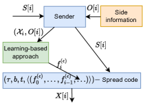
Figure 4: Illustration of the $(\tau,b,t)-$Spread ML Code. A learning-based approach is used to determine a policy, $f^{(\epsilon)}_{i}$, during the $i$th time slot, which is then used by the $\left(\tau,b,t,\left\langle f^{(\epsilon)}_{i}\mid i\in[t]\right\rangle\right)-$Spread Code.

To determine how to spread message symbols, we use the side information of $\mathcal{S}$ samples the distribution of the sizes of the future message packets, which was defined in Eq. (1) as $\big{\langle}(k_{i+1}^{(j)},\ldots,k_{t}^{(j)})\sim D_{k_{0},\ldots,k_{i}}\mid j\in\{0,\ldots,\mathcal{S}-1\}\big{\rangle}$. We use a similar technique to empirical risk minimization over the $\mathcal{S}$ samples to set $f^{(\epsilon)}_{i}$ to the value leading to lowest expected number of symbols being sent by a rate-optimal offline code. Specifically, for any $i=0,\ldots,t$, $j\in[\mathcal{S}-1]$ and $l\in[k_{i}]$, let

$$z_{i,j,l}=\sum_{r=i}^{t}p^{(IP)}_{r},$$

where $p^{(IP)}_{i},\ldots,p^{(IP)}_{t}$ are variables used by the IP of Algorithm 2 given $X[0],\ldots,X[i-1],$ and $f^{(IP)}_{i}=l$. Then

$$f^{(\epsilon)}_{i}=\arg\min_{l\in[k_{i}]}\frac{1}{\mathcal{S}-1}\sum_{j\in[\mathcal{S}-1]}z_{i,j,l}.$$ (27)

We demonstrate how $f^{(\epsilon)}_{i}$ is defined in Figure 5.

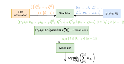
Figure 5: Illustration of the learning-based approach (green) to determine how to spread message symbols.

The key observation to interpret the choice of $f^{(\epsilon)}_{i}$ is that the number of parity symbols sent corresponding to message packet $S[i]$, namely $p_{i+\tau}$, is monotonically non-decreasing as $f^{(\epsilon)}_{i}$ increases. Thus, smaller values of $f^{(\epsilon)}_{i}$ lead to smaller values of $p_{i+\tau}$, which exploits the parity symbols already sent before time slot $(i+\tau)$. This strategy is effective when the next several message packets are likely small. Therefore, a small $P[i+\tau]$ suffices to ensure that the next several message packets are recovered when some of $X[i+2],\ldots,X[i+\tau-1]$ are lost. In contrast, larger values of $f^{(\epsilon)}_{i}$ promote larger values of $p_{i+\tau}$, which is suitable when the next several message packets are likely to be large. Hence, a large $P[i+\tau]$ will not go to waste even if a burst starts after receiving $S[i]$.

To show that the $(\tau,b,t)-$Spread ML Code is approximately rate optimal, we analyze the number of extra symbols it sends compared to an optimal scheme as follows.

Definition 3 (Regret)

The regret, $\mathcal{R}_{k_{i},\ldots,k_{t}}\left(f^{(\epsilon)}_{i}\right)$, for the message packet size sequence $k_{0},\ldots,k_{t}$ is the number of extra symbols sent under Algorithm 2 when $f^{(\epsilon)}_{i}$ is used compared to the best offline policy, $f_{i}^{\prime}$.

The number of extra symbols sent compared to an optimal offline scheme is $\sum_{i=0}^{t}\mathcal{R}_{k_{i},\ldots,k_{t}}\left(f^{(\epsilon)}_{i}\right)$, as is shown next for completeness.

Lemma 4

For message packet size sequence $k_{0},\ldots,k_{t}$, the $(\tau,b,t)-$Spread ML Code transmits $\sum_{i=0}^{t}\mathcal{R}_{k_{i},\ldots,k_{t}}\left(f_{i}\right)$ more symbols than a scheme meeting the offline-optimal-rate.

Proof:

We can sequentially improve the $(\tau,b,t)-$Spread ML Code for $i=t-2\tau,\ldots,2\tau$ by switching $f^{(\epsilon)}_{j}$ for $j\in\{i,\ldots,t\}$ to the one computed by Algorithm 2 given $f^{(\epsilon)}_{0},\ldots,f^{(\epsilon)}_{i-1},p_{0},\ldots,p_{i-1}$. For each value of $i$, the improvement in total number of symbols sent is $\mathcal{R}_{k_{i},\ldots,k_{t}}\left(f_{i}\right)$ by Definition 3. After reaching $i=2\tau$, the output is simply Algorithm 2, as $k_{0}=0,\ldots,k_{2\tau-1}=0$. ∎

Next, we bound the expected regret of the $(\tau,b,t)-$Spread ML Code from spreading message symbols for any time slot.

Lemma 5

For any $(\tau,b,t)$, $\mathcal{S}\geq\sqrt{\ln(\frac{8m^{2}}{\epsilon})}\frac{2\sqrt{2}m^{3}}{\epsilon}$ samples from the side information, where $m$ is the maximum size of a message packet, $i\in[t]$, $k_{0},\ldots,k_{i-1},$ and $f_{i}^{\prime}\in[k_{i}]$,

$$\mathrm{E}_{k_{i+1},\ldots,k_{t}}\left[\mathcal{R}_{k_{i},\ldots,k_{t}}\left(f^{(\epsilon)}_{i}\right)-\mathcal{R}_{k_{i},\ldots,k_{t}}\left(f_{i}^{\prime}\right)\right]\leq\epsilon.$$ (28)

Proof:

If $k_{i}=0$, $f_{i}=f^{(\epsilon)}_{i}$, concluding the proof. Otherwise, the choice of $f^{(\epsilon)}_{i}$ leads to sending $k_{i}$ extra parity symbols in $X[i+\tau]$ compared to an optimal scheme, so

$$\mathcal{R}_{k_{i},\ldots,k_{t}}\left(f^{(\epsilon)}_{i}\right)\leq m$$ (29)

and

$$\mathrm{E}_{k_{i+1},\ldots,k_{t}}\left[\mathcal{R}_{k_{i},\ldots,k_{t}}\left(f^{(\epsilon)}_{i}\right)\right]\leq m,\>\mathrm{Var}_{k_{i+1},\ldots,k_{t}}\left(\mathcal{R}_{k_{i},\ldots,k_{t}}\left(f^{(\epsilon)}_{i}\right)\right)\leq m^{2}.$$

At a high level, we apply the Hoeffding bound [59] to show that the expected regret for each possible policy is well approximated using the empirical mean over the $\mathcal{S}$ samples from the side information. The unlikely event that the expected value deviates greatly from the mean will have negligible impact due to Eq. (29).

Next, we use $O[i]$ to determine the values of $\mathcal{S}$ random variables, $\left(z_{i,j,0},\ldots,z_{i,j,\mathcal{S}-1}\right)$, equaling $\mathcal{R}_{k_{i},\ldots,k_{t}}(j)$ in distribution. The empirical mean, $\frac{1}{\mathcal{S}}\sum_{l=0}^{\mathcal{S}-1}z_{i,j,l}$, is used to estimate $\mathrm{E}_{k_{i},\ldots,k_{t}}[\mathcal{R}_{k_{i},\ldots,k_{t}}(j)]$. By the Hoeffding bound [59],

$$\left|\frac{1}{\mathcal{S}}\left(\sum_{l=0}^{\mathcal{S}-1}z_{i,j,l}\right)-\mathrm{E}_{k_{0},\ldots,k_{t}}[\mathcal{R}_{k_{i},\ldots,k_{t}}(j)]\right|<\epsilon_{\dagger}$$

with probability at least

$$\left(1-2e^{-\frac{2\mathcal{S}^{2}(\epsilon_{\dagger})^{2}}{m^{2}}}\right)\geq(1-\delta)$$

as long as

$$\frac{\delta}{2} \geq e^{-\frac{2\mathcal{S}^{2}(\epsilon_{\dagger})^{2}}{m^{2}}}$$

$$\frac{2\mathcal{S}^{2}(\epsilon_{\dagger})^{2}}{m^{2}} \geq\ln\left(\frac{2}{\delta}\right)$$

$$\mathcal{S}^{2} \geq\ln\left(\frac{2}{\delta}\right)\frac{m^{2}}{2(\epsilon_{\dagger})^{2}}$$

$$\mathcal{S} \geq\sqrt{\ln\left(\frac{2}{\delta}\right)}\frac{m}{\sqrt{2}\epsilon_{\dagger}}.$$

Using $\epsilon_{\dagger}=\delta=\frac{\epsilon}{4m^{2}}$ and applying the union bound over the at most $m$ values of $k_{i}$ shows with probability $(1-m\delta)$ for all $j\in[k_{i}]$,

$$\left|\frac{1}{\mathcal{S}}\left(\sum_{l=0}^{\mathcal{S}-1}z_{i,j,l}\right)-\mathrm{E}_{k_{0},\ldots,k_{t}}\left[\mathcal{R}_{k_{i},\ldots,k_{t}}\right]\left(f^{(\epsilon)}_{i,j}\right)]\right|<\epsilon_{\dagger}.$$ (30)

We set $f^{(\epsilon)}_{i}$ according to Eq. (27) as

$$f^{(\epsilon)}_{i}=\arg\min_{j}\frac{1}{\mathcal{S}}\sum_{l=0}^{\mathcal{S}-1}z_{i,j,l}.$$

With probability $(1-m\delta)$ Eq. (30) holds, leading to

$$\mathrm{E}_{k_{i},\ldots,k_{t}}\left[\mathcal{R}_{k_{i},\ldots,k_{t}}\left(f^{(\epsilon)}_{i}\right)-\mathcal{R}_{k_{i},\ldots,k_{t}}\left(f_{i}^{\prime}\right)\right]\leq$$ (31)

$$\mathrm{E}_{k_{i},\ldots,k_{t}}\left[\mathcal{R}_{k_{i},\ldots,k_{t}}\left(f^{(\epsilon)}_{i}\right)-\mathcal{R}_{k_{i},\ldots,k_{t}}\left(f_{i}^{\prime}\right)\right]+\left(\frac{1}{\mathcal{S}}\left(\sum_{l=0}^{\mathcal{S}-1}z_{i,f_{i}^{\prime},l}\right)-\frac{1}{\mathcal{S}}\left(\sum_{l=0}^{\mathcal{S}-1}z_{i,f^{(\epsilon)}_{i},l}\right)\right)\leq$$

$$\left(\mathrm{E}_{k_{i},\ldots,k_{t}}\left[\left(\mathcal{R}_{k_{i},\ldots,k_{t}}\left(f^{(\epsilon)}_{i}\right)\right]-\frac{1}{\mathcal{S}}\left(\sum_{l=0}^{\mathcal{S}-1}z_{i,f^{(\epsilon)}_{i},l}\right)\right)\right)+\left(\left(\frac{1}{\mathcal{S}}\left(\sum_{l=0}^{\mathcal{S}-1}z_{i,f_{i}^{\prime},l}\right)-\mathrm{E}_{k_{i},\ldots,k_{t}}\left[\mathcal{R}_{k_{i},\ldots,k_{t}}\left(f_{i}^{\prime}\right)\right]\right)\right)\leq$$

$$\left|\mathrm{E}_{k_{i},\ldots,k_{t}}\left[\mathcal{R}_{k_{i},\ldots,k_{t}}\left(f^{(\epsilon)}_{i}\right)\right]-\frac{1}{\mathcal{S}}\left(\sum_{l=0}^{\mathcal{S}-1}z_{i,f^{(\epsilon)}_{i},l}\right)\right|+\left|\left(\frac{1}{\mathcal{S}}\left(\sum_{l=0}^{\mathcal{S}-1}z_{i,f_{i}^{\prime},l}\right)-\mathrm{E}_{k_{i},\ldots,k_{t}}\left[\mathcal{R}_{k_{i},\ldots,k_{t}}\left(f_{i}^{\prime}\right)\right]\right)\right|\leq 2\epsilon_{\dagger},$$

which used the fact that Eq. (27) led to

$$\frac{1}{\mathcal{S}}\left(\sum_{l=0}^{\mathcal{S}-1}z_{i,f_{i}^{\prime},l}\right)\geq\frac{1}{\mathcal{S}}\left(\sum_{l=0}^{\mathcal{S}-1}z_{i,f^{(\epsilon)}_{i},l}\right).$$

Otherwise, with probability $m\delta$

$$\mathrm{E}_{k_{i},\ldots,k_{t}}\left[\mathcal{R}_{k_{i},\ldots,k_{t}}(f^{(\epsilon)}_{i})-\mathcal{R}_{k_{i},\ldots,k_{t}}\left(f_{i}^{\prime}\right)\right]\leq m.$$ (32)

Combining Eqs. (31) and (32) leads to

$$\mathrm{E}_{k_{i},\ldots,k_{t}}\left[\mathcal{R}_{k_{i},\ldots,k_{t}}(f^{(\epsilon)}_{i})-\mathcal{R}_{k_{i},\ldots,k_{t}}\left(f_{i}^{\prime}\right)\right]\leq\delta m^{2}+2\epsilon_{\dagger}\leq\epsilon.$$

∎

Finally, we show that the expected online-optimal-rate, denoted as “$R^{(\mathrm{E},Opt)}$,” is within $\epsilon$ of the expected rate of the $(\tau,b,t)-$Spread ML Code, denoted as

$$R^{(\mathrm{E})}=\mathrm{E}_{k_{0},\ldots,k_{t}}\left[\frac{\sum_{i=0}^{t}k_{i}}{\sum_{i=0}^{t}k_{i}+p_{i}}\right].$$ (33)

Theorem 2

For any $(\tau,b,t)$ and for $\mathcal{S}\geq\sqrt{\ln(\frac{8m^{2}}{\epsilon})}\frac{2\sqrt{2}m^{3}}{\epsilon}$ samples from the side information, where $m$ is the maximum size of a message packet, $(R^{(\mathrm{E},Opt)}-R^{(\mathrm{E})})<\epsilon$.

Proof:

We consider an online scheme with the optimal expected rate, namely the $\left(\tau,b,t,\left\langle f_{i}^{\prime}\mid i\in[t]\right\rangle\right)-$Spread Code, which must exist by Lemma 3. Let $n_{i}$ be the number of symbols sent in $X[i]$ under the optimal scheme and

$$n_{\epsilon} =\sum_{i=0}^{t}\mathcal{R}_{k_{i},\ldots,k_{t}}\left(f^{(\epsilon)}_{i}\right)-\mathcal{R}_{k_{i},\ldots,k_{t}}\left(f_{i}^{\prime}\right)$$ (34)

be the number of additional symbols sent under the $\left(\tau,b,t,\left\langle f_{i}^{\prime}\mid i\in[t]\right\rangle\right)-$Spread Code.

By definition

$$R^{(\mathrm{E},Opt)}-R^{(\mathrm{E})} \leq\mathrm{E}_{k_{0},\ldots,k_{t}}\left[\left|\frac{\sum_{i=0}^{t}k_{i}}{\sum_{i=0}^{t}n_{i}}-\frac{\sum_{i=0}^{t}k_{i}}{n_{\epsilon}+\sum_{i=0}^{t}n_{i}}\right|\right]$$ (35)

$$\leq\mathrm{E}_{k_{0},\ldots,k_{t}}\left[\left|\frac{|n_{\epsilon}|\sum_{i=0}^{t}k_{i}}{\left(\sum_{i=0}^{t}n_{i}\right)\left(n_{\epsilon}+\sum_{i=0}^{t}n_{i}\right)}\right|\right]$$

$$\leq\mathrm{E}_{k_{0},\ldots,k_{t}}\left[\frac{|n_{\epsilon}|}{\sum_{i=0}^{t}n_{i}}\right]$$ (36)

$$\leq\mathrm{E}_{k_{0},\ldots,k_{t}}\left[\frac{|n_{\epsilon}|}{\sum_{i=0}^{t}\mathds{1}[k_{i}>0]}\right],$$ (37)

where Eq. (36) follows from sending $\sum_{i=0}^{t}n_{i}\geq\sum_{i=0}^{t}k_{i}$ symbols to satisfy the lossless-delay constraint, and Eq. (37) follows from $\sum_{i=0}^{t}k_{i}\geq\sum_{i=0}^{t}\mathds{1}[k_{i}>0]$.

If $k_{i}=0$, then $\mathcal{R}_{k_{i},\ldots,k_{t}}\left(f^{(\epsilon)}_{i}\right)=\mathcal{R}_{k_{i},\ldots,k_{t}}\left(f_{i}^{\prime}\right)=0$. Thus, we can simplify Eq. (34) as

$$n_{\epsilon}=\sum_{i=0}^{t}\mathds{1}[k_{i}>0]\left(\mathcal{R}_{k_{i},\ldots,k_{t}}\left(f^{(\epsilon)}_{i}\right)-\mathcal{R}_{k_{i},\ldots,k_{t}}\left(f_{i}^{\prime}\right)\right).$$ (38)

Applying Eq. (38) to Eqs. (35) and (37) leads to

$$R^{(\mathrm{E},Opt)}-R^{(\mathrm{E})} \leq\mathrm{E}_{k_{0},\ldots,k_{t}}\left[\frac{\sum_{i=0}^{t}\mathds{1}[k_{i}>0]\left(\mathcal{R}_{k_{i},\ldots,k_{t}}\left(f^{(\epsilon)}_{i}\right)-\mathcal{R}_{k_{i},\ldots,k_{t}}\left(f_{i}^{\prime}\right)\right)}{\sum_{i=0}^{t}\mathds{1}[k_{i}>0]}\right]$$

$$\leq\max_{i\in[t]}\mathrm{E}_{k_{0},\ldots,k_{t}}\left[\mathcal{R}_{k_{i},\ldots,k_{t}}\left(f^{(\epsilon)}_{i}\right)-\mathcal{R}_{k_{i},\ldots,k_{t}}\left(f_{i}^{\prime}\right)\right]$$

$$=\max_{i\in[t]}\mathrm{E}_{k_{0},\ldots,k_{i-1}}\left[\mathrm{E}_{k_{i},\ldots,k_{t}}\left[\mathcal{R}_{k_{i},\ldots,k_{t}}\left(f^{(\epsilon)}_{i}\right)-\mathcal{R}_{k_{i},\ldots,k_{t}}\left(f_{i}^{\prime}\right)\right]\right]$$

As such, it suffices to show for all $i\in[t]$ that

$$\mathrm{E}_{k_{0},\ldots,k_{i-1}}\left[\mathrm{E}_{k_{i},\ldots,k_{t}}\left[\mathcal{R}_{k_{i},\ldots,k_{t}}\left(f^{(\epsilon)}_{i}\right)-\mathcal{R}_{k_{i},\ldots,k_{t}}\left(f_{i}^{\prime}\right)\right]\right]\leq\epsilon.$$ (39)

Because $\mathcal{S}\geq\sqrt{\ln(\frac{8m^{2}}{\epsilon})}\frac{2\sqrt{2}m^{3}}{\epsilon}$, Lemma 5 guarantees for any $k_{0},\ldots,k_{i-1}$,

$$\mathrm{E}_{k_{i},\ldots,k_{t}}\left[\mathcal{R}_{k_{i},\ldots,k_{t}}\left(f^{(\epsilon)}_{i}\right)-\mathcal{R}_{k_{i},\ldots,k_{t}}\left(f_{i}^{\prime}\right)\right]\leq\epsilon,$$

concluding the proof. ∎

We have designed an online code that uses a black box algorithm to determine how to spread message symbols and bounded how close the rate is to optimal based on the regret due to the choices of how to spread. To show that the code is approximately rate optimal, we presented an explicit learning-based approach of leveraging samples to the distribution of the sizes of future message packets to spread message symbols (i.e., Eq. (27)) and showed in Lemma 5 that it has a sufficiently small expected regret. More generally, any criteria with a sufficiently small expected regret could be used, leading to the following result.

Corollary 2

Theorem 2 holds when any criteria for spreading message symbols is substituted for Eq. (27) if the criteria satisfies Eq. (28) for all $i\in[t]$, $k_{0},\ldots,k_{t},$ and $f_{i}^{\prime}\in[k_{i}]$.

VI Conclusion

Inspired by the growing field of learning-augmented algorithms, this work introduces a new methodology for constructing online streaming codes that combines machine learning with algebraic coding theory tools. The approach is to (a) isolate the component that can benefit from machine learning, (b) solve the offline version of the problem by integrating optimization with algebraic coding theory techniques, and (c) convert the offline scheme into an online one using a learning-based approach. This strategy is applicable beyond the setting considered in this paper, including numerous other settings for real-time streaming communication.

References

- [1] M. Rudow and K. Rashmi, “Learning-based streaming codes are approximately optimal for variable-size messages,” to be published 2022 IEEE International Symposium on Information Theory (ISIT). IEEE, 2022.
- [2] A. Badr, A. Khisti, W. Tan, and J. Apostolopoulos, “Perfecting protection for interactive multimedia: A survey of forward error correction for low-delay interactive applications,” IEEE Signal Processing Magazine, vol. 34, no. 2, pp. 95–113, March 2017.
- [3] E. Martinian and C. . W. Sundberg, “Burst erasure correction codes with low decoding delay,” IEEE Trans. Inf. Theory, vol. 50, no. 10, pp. 2494–2502, Oct 2004.
- [4] E. Martinian and M. Trott, “Delay-optimal burst erasure code construction,” in ISIT, June 2007, pp. 1006–1010.
- [5] A. Badr, P. Patil, A. Khisti, W. Tan, and J. Apostolopoulos, “Layered constructions for low-delay streaming codes,” IEEE Trans. Inf. Theory, vol. 63, no. 1, pp. 111–141, Jan 2017.
- [6] S. L. Fong, A. Khisti, B. Li, W. Tan, X. Zhu, and J. Apostolopoulos, “Optimal streaming codes for channels with burst and arbitrary erasures,” IEEE Trans. Inf. Theory, vol. 65, no. 7, pp. 4274–4292, July 2019.
- [7] M. N. Krishnan and P. V. Kumar, “Rate-optimal streaming codes for channels with burst and isolated erasures,” in ISIT, June 2018, pp. 1809–1813.
- [8] M. N. Krishnan, D. Shukla, and P. V. Kumar, “Rate-optimal streaming codes for channels with burst and random erasures,” IEEE Trans. Inf. Theory, vol. 66, no. 8, pp. 4869–4891, 2020.
- [9] E. Domanovitz, S. L. Fong, and A. Khisti, “An explicit rate-optimal streaming code for channels with burst and arbitrary erasures,” IEEE Transactions on Information Theory, vol. 68, no. 1, pp. 47–65, 2022.
- [10] A. Badr, D. Lui, A. Khisti, W. Tan, X. Zhu, and J. Apostolopoulos, “Multiplexed coding for multiple streams with different decoding delays,” IEEE Trans. Inf. Theory, vol. 64, no. 6, pp. 4365–4378, June 2018.
- [11] S. L. Fong, A. Khisti, B. Li, W. Tan, X. Zhu, and J. Apostolopoulos, “Optimal multiplexed erasure codes for streaming messages with different decoding delays,” IEEE Trans. Inf. Theory, vol. 66, no. 7, pp. 4007–4018, 2020.
- [12] A. Badr, A. Khisti, and E. Martinian, “Diversity embedded streaming erasure codes (de-sco): Constructions and optimality,” IEEE J. Sel. Areas Inf. Theory, vol. 29, no. 5, pp. 1042–1054, May 2011.
- [13] A. Badr, D. Lui, and A. Khisti, “Streaming codes for multicast over burst erasure channels,” IEEE Trans. Inf. Theory, vol. 61, no. 8, pp. 4181–4208, Aug 2015.
- [14] M. Haghifam, M. N. Krishnan, A. Khisti, X. Zhu, W.-T. Tan, and J. Apostolopoulos, “On streaming codes with unequal error protection,” IEEE J. Sel. Areas Inf. Theory, 2021.
- [15] N. Adler and Y. Cassuto, “Burst-erasure correcting codes with optimal average delay,” IEEE Trans. Inf. Theory, vol. 63, no. 5, pp. 2848–2865, May 2017.
- [16] D. Leong and T. Ho, “Erasure coding for real-time streaming,” in ISIT, July 2012, pp. 289–293.
- [17] D. Leong, A. Qureshi, and T. Ho, “On coding for real-time streaming under packet erasures,” in ISIT, July 2013, pp. 1012–1016.
- [18] A. Badr, A. Khisti, W. Tan, and J. Apostolopoulos, “Streaming codes with partial recovery over channels with burst and isolated erasures,” IEEE J. Sel. Topics Signal Process., vol. 9, no. 3, pp. 501–516, April 2015.
- [19] S. L. Fong, A. Khisti, B. Li, W.-T. Tan, X. Zhu, and J. Apostolopoulos, “Optimal streaming erasure codes over the three-node relay network,” IEEE Trans. Inf. Theory, vol. 66, no. 5, pp. 2696–2712, 2020.
- [20] A. Badr, A. Khisti, W.-t. Tan, X. Zhu, and J. Apostolopoulos, “Fec for voip using dual-delay streaming codes,” in IEEE INFOCOM 2017 - IEEE Conference on Computer Communications, 2017, pp. 1–9.
- [21] Z. Li, A. Khisti, and B. Girod, “Correcting erasure bursts with minimum decoding delay,” in Conf. Rec. Asilomar Conf. Signals Syst. Comput., Nov 2011, pp. 33–39.
- [22] Y. Wei and T. Ho, “On prioritized coding for real-time streaming under packet erasures,” in Allerton. IEEE, 2013, pp. 327–334.
- [23] M. N. Krishnan, V. Ramkumar, M. Vajha, and P. V. Kumar, “Simple streaming codes for reliable, low-latency communication,” IEEE Communications Letters, pp. 1–1, 2019.
- [24] V. Ramkumar, M. Vajha, M. N. Krishnan, and P. Vijay Kumar, “Staggered diagonal embedding based linear field size streaming codes,” pp. 503–508, 2020.
- [25] P.-W. Su, Y.-C. Huang, S.-C. Lin, I.-H. Wang, and C.-C. Wang, “Random linear streaming codes in the finite memory length and decoding deadline regime,” in ISIT, 2021, pp. 730–735.
- [26] M. Rudow and K. Rashmi, “Streaming codes for variable-size messages,” IEEE Transactions on Information Theory, pp. 1–1, 2022.
- [27] ——, “Online versus offline rate in streaming codes for variable-size messages,” in ISIT. IEEE, 2020, pp. 509–514.
- [28] T. Lykouris and S. Vassilvtiskii, “Competitive caching with machine learned advice,” in International Conference on Machine Learning. PMLR, 2018, pp. 3296–3305.
- [29] A. Antoniadis, C. Coester, M. Elias, A. Polak, and B. Simon, “Online metric algorithms with untrusted predictions,” in International Conference on Machine Learning. PMLR, 2020, pp. 345–355.
- [30] M. Mitzenmacher, “A model for learned bloom filters and optimizing by sandwiching,” Advances in Neural Information Processing Systems, vol. 31, 2018.
- [31] T. Kraska, A. Beutel, E. H. Chi, J. Dean, and N. Polyzotis, “The case for learned index structures,” in Proceedings of the 2018 international conference on management of data, 2018, pp. 489–504.
- [32] S. Lattanzi, T. Lavastida, B. Moseley, and S. Vassilvitskii, “Online scheduling via learned weights,” in Proceedings of the Fourteenth Annual ACM-SIAM Symposium on Discrete Algorithms. SIAM, 2020, pp. 1859–1877.
- [33] É. Bamas, A. Maggiori, and O. Svensson, “The primal-dual method for learning augmented algorithms,” Advances in Neural Information Processing Systems, vol. 33, pp. 20 083–20 094, 2020.
- [34] M. Mitzenmacher and S. Vassilvitskii, “Algorithms with predictions,” arXiv preprint arXiv:2006.09123, 2020.
- [35] C.-Y. Hsu, P. Indyk, D. Katabi, and A. Vakilian, “Learning-based frequency estimation algorithms.” in International Conference on Learning Representations, 2019.
- [36] T. Jiang, Y. Li, H. Lin, Y. Ruan, and D. P. Woodruff, “Learning-augmented data stream algorithms,” in International Conference on Learning Representations, 2019.
- [37] K. Anand, R. Ge, and D. Panigrahi, “Customizing ml predictions for online algorithms,” in International Conference on Machine Learning. PMLR, 2020, pp. 303–313.
- [38] T. Gruber, S. Cammerer, J. Hoydis, and S. t. Brink, “On deep learning-based channel decoding,” in 2017 51st Annual Conference on Information Sciences and Systems (CISS), 2017, pp. 1–6.
- [39] E. Nachmani, E. Marciano, L. Lugosch, W. J. Gross, D. Burshtein, and Y. Be’ery, “Deep learning methods for improved decoding of linear codes,” IEEE J. Sel. Topics Signal Process., vol. 12, no. 1, pp. 119–131, 2018.
- [40] L. Lugosch and W. J. Gross, “Neural offset min-sum decoding,” in ISIT, 2017, pp. 1361–1365.
- [41] S. Dörner, S. Cammerer, J. Hoydis, and S. t. Brink, “Deep learning based communication over the air,” IEEE J. Sel. Topics Signal Process., vol. 12, no. 1, pp. 132–143, 2018.
- [42] S. Cammerer, T. Gruber, J. Hoydis, and S. ten Brink, “Scaling deep learning-based decoding of polar codes via partitioning,” in GLOBECOM 2017 - 2017 IEEE Global Communications Conference, 2017, pp. 1–6.
- [43] Y. Jiang, H. Kim, H. Asnani, S. Kannan, S. Oh, and P. Viswanath, “Turbo autoencoder: Deep learning based channel codes for point-to-point communication channels,” Advances in neural information processing systems, vol. 32, pp. 2758–2768, 2019.
- [44] Y. Jiang, S. Kannan, H. Kim, S. Oh, H. Asnani, and P. Viswanath, “Deepturbo: Deep turbo decoder,” in 2019 IEEE 20th International Workshop on Signal Processing Advances in Wireless Communications (SPAWC). IEEE, 2019, pp. 1–5.
- [45] E. Nachmani and L. Wolf, “Hyper-graph-network decoders for block codes,” Advances in Neural Information Processing Systems, vol. 32, pp. 2329–2339, 2019.
- [46] A. V. Makkuva, X. Liu, M. V. Jamali, H. Mahdavifar, S. Oh, and P. Viswanath, “Ko codes: inventing nonlinear encoding and decoding for reliable wireless communication via deep-learning,” in International Conference on Machine Learning. PMLR, 2021, pp. 7368–7378.
- [47] H. Kim, Y. Jiang, S. Kannan, S. Oh, and P. Viswanath, “Deepcode: Feedback codes via deep learning,” Advances in neural information processing systems, vol. 31, 2018.
- [48] D. B. Kurka and D. Gündüz, “Deepjscc-f: Deep joint source-channel coding of images with feedback,” IEEE J. Sel. Areas Inf. Theory, vol. 1, no. 1, pp. 178–193, 2020.
- [49] J. Kosaian, K. Rashmi, and S. Venkataraman, “Parity models: erasure-coded resilience for prediction serving systems,” in Proceedings of the 27th ACM Symposium on Operating Systems Principles, 2019.
- [50] J. Kosaian, K. V. Rashmi, and S. Venkataraman, “Learning-based coded computation,” IEEE J. Sel. Areas Inf. Theory, vol. 1, no. 1, pp. 227–236, 2020.
- [51] H. V. Krishna Giri Narra, Z. Lin, G. Ananthanarayanan, S. Avestimehr, and M. Annavaram, “Collage inference: Using coded redundancy for lowering latency variation in distributed image classification systems,” in 2020 IEEE 40th International Conference on Distributed Computing Systems (ICDCS), 2020, pp. 453–463.
- [52] Y.-S. Jeon, S.-N. Hong, and N. Lee, “Blind detection for mimo systems with low-resolution adcs using supervised learning,” in 2017 IEEE International Conference on Communications (ICC), 2017, pp. 1–6.
- [53] N. Samuel, T. Diskin, and A. Wiesel, “Learning to detect,” EEE Trans. Signal Process., vol. 67, no. 10, pp. 2554–2564, 2019.
- [54] N. Farsad and A. Goldsmith, “Detection algorithms for communication systems using deep learning,” 2017.
- [55] G. Gui, H. Huang, Y. Song, and H. Sari, “Deep learning for an effective nonorthogonal multiple access scheme,” IEEE Trans. Veh. Technol., vol. 67, no. 9, pp. 8440–8450, 2018.
- [56] T. O’Shea and J. Hoydis, “An introduction to deep learning for the physical layer,” IEEE Trans. Cogn. Commun. Netw., vol. 3, no. 4, pp. 563–575, 2017.
- [57] T. J. O’Shea, K. Karra, and T. C. Clancy, “Learning to communicate: Channel auto-encoders, domain specific regularizers, and attention,” in 2016 IEEE Int. Symp. Signal Process. Inf. Technol., 2016, pp. 223–228.
- [58] K. Choi, K. Tatwawadi, T. Weissman, and S. Ermon, “Necst: neural joint source-channel coding,” 2018.
- [59] W. Hoeffding, Probability Inequalities for sums of Bounded Random Variables. New York, NY: Springer New York, 1994, pp. 409–426. [Online]. Available: https://doi.org/10.1007/978-1-4612-0865-5_26