Do Neural Networks Compress
Manifolds Optimally?

Abstract

Artifical Neural-Network-based (ANN-based) lossy compressors have recently obtained striking results on several sources. Their success may be ascribed to an ability to identify the structure of low-dimensional manifolds in high-dimensional ambient spaces. Indeed, prior work has shown that ANN-based compressors can achieve the optimal entropy-distortion curve for some such sources. In contrast, we determine the optimal entropy-distortion tradeoffs for two low-dimensional manifolds with circular structure and show that state-of-the-art ANN-based compressors fail to optimally compress them.

I Introduction

Stochastically-trained Artificial Neural-Network-based (ANN-based) lossy compressors are the state-of-the-art for various types of sources, most notably images [1, 2, 3]. One particularly successful framework for using ANNs for lossy compression, which is the focus of this paper, creates the compressed representation by quantizing the latent variables in an autoencoder-like architecture [4]. One can view this as similar to the transform-based coding approach that underpins JPEG and other standards, except that the transforms are implemented by multilayer perceptrons and can therefore be nonlinear. These ANN-based compressors outperform linear-transform-based methods, even under a mean-squared-error (MSE) distortion measure [1]. Since the latter is provably near-optimal for stationary Gaussian sources under an MSE distortion constraint, ANN-based compressors are evidently able to exploit non-Gaussianity in sources.

Given that ensembles of images have long been suspected to live on low-dimensional manifolds in pixel-space, it is natural to conjecture that ANN-based compressors are adept at compressing sources that exhibit low-dimensional manifold structure in a high-dimensional ambient space. Previous work [5] considered a particular random process (the “sawbridge”) over $[0,1]$ exhibiting this structure and found that stochastically-trained ANNs indeed compress the process optimally.

We consider the random process obtained by applying a random cyclic shift to the function $t\mapsto t-1/2$ over $[0,1]$. We call the resulting process the ramp. We characterize the entropy-distortion function for this process under an MSE distortion constraint. Despite the considerable similarities between the ramp and the sawbridge, we find that stochastically-trained ANN-based compressors fail to compress the ramp optimally at high-SNR. The difficulty stems from the fact that, unlike the sawbridge, the set of ramp realizations forms a closed loop in function space, which creates a topological challenge related to the impossibility of mapping a circle to a segment in a continuous and invertible way [6, Chap 2. Ex. 7]. To illustrate this issue in arguably its simplest form, we begin by considering the problem of compressing the unit circle in two-dimensions. We characterize the entropy-distortion function and again find that stochastically-trained ANNs are suboptimal at high rates.

II Preliminaries

For a source $X$ in a space ${\cal M}$, we define an encoder and its entropy and distortion. In this paper ${\cal M}$ will be either $L^{2}\left[0,1\right]$ or $\mathbb{R}^{2}$. In both cases, conditional expectations and norms are well-defined.

Definition 1.

An encoder is a mapping $f:{\cal M}\mapsto\mathbb{N}$. Its entropy and distortion are given by

$$H(f) =\sum\limits_{i\in\mathbb{N}}-\Pr\left(f(X)=i\right)\log{\left({\Pr{\left({f(X)=i}\right)}}\right)}$$

$$D(f) =\mathbb{E}{\left[{\left\lVert X-\mathbb{E}{\left[{X\mid f(X)}\right]}\right\rVert^{2}}\right]},$$

respectively.

Note in particular that we consider mean squared error as the distortion measure. We shall characterize optimal compression performance via the entropy-distortion function.

Definition 2.

The entropy-distortion function of $X$ is

$$E(D)= \inf\limits_{f}H(f)$$

$$\textrm{s.t. }D(f)\leq D.$$

We consider the entropy-distortion function instead of the more-conventional rate-distortion function [7, Theorem 10.2.1] because ANN-based compressors optimize entropy, which is known to be a lower bound to the expected codeword length under optimal, one-shot prefix-free encoding [7, Theorem 5.4.1]

III The Circle

The circle is a 2-D source with a 1-D latent variable.

$$\theta\sim\text{Unif}\left[0,2\pi\right),{{\overrightarrow{Z}}}=\left(\cos\theta,\sin\theta\right).$$ (1)

We first derive its optimal entropy-distortion tradeoff and then analyze the performance of ANN-based compressors.

III-A The Optimal Tradeoff

Theorem 3.

For the circle, if $D\geq 1$, $E_{\text{c}}(D)=0$. If $0<D<1$, then

$$E_{\text{c}}(D)=\inf\limits_{\left\{\theta_{i}\right\}_{i=1}^{\infty}}\quad- \sum\limits_{i}^{\infty}\frac{\theta_{i}}{2\pi}\log{\left({\frac{\theta_{i}}{2\pi}}\right)}$$

s.t. $$\sum\limits_{i=1}^{\infty}\frac{\theta_{i}}{2\pi}\left(1-\operatorname{sinc}^{2}{\left({\frac{\theta_{i}}{2}}\right)}\right)\leq D,$$

$$\sum\limits_{i=1}^{\infty}\theta_{i}=2\pi,\theta_{i}\geq 0\text{ for all i},$$

where

$$\operatorname{sinc}(x)=\begin{cases}\frac{\sin(x)}{x}&\text{if $x\neq 0$}\\ 1&\text{otherwise}.\end{cases}$$ (2)

Proof.

Let $f:\mathbb{R}^{2}\mapsto\mathbb{N}$ be an encoder. For the circle source, an encoder $f$ can be alternatively represented as a function of the angle $\theta\in\left[0,2\pi\right)$ as $h(\theta)=f{\left({\left[\cos\theta,\sin\theta\right]}\right)}$. Let ${\cal C}$ denote the unit circle and define $C_{i}\stackrel{{\scriptstyle\text{def}}}{{=}}{\cal C}\cap f^{-1}(i)$ and $\Theta_{i}\stackrel{{\scriptstyle\text{def}}}{{=}}\left[0,2\pi\right)\cap h^{-1}(i)$. $C_{i}$ is said to be contiguous if $\Theta_{i}$ is an interval or if it is of the form $\left[0,\theta_{1}\right]\cup\left[2\pi-\theta_{2},2\pi\right)$. Let $\mu(C_{i})$ be the Lebesgue of $C_{i}$. The entropy and distortion are given by

$$H(f) =\sum\limits_{i=1}^{\infty}-\frac{\mu(C_{i})}{2\pi}\log{\left({\frac{\mu(C_{i})}{2\pi}}\right)},$$

$$D(f) =\sum\limits_{i=1}^{\infty}\frac{\mu(C_{i})}{2\pi}\mathbb{E}{\left[{\left\lVert{{\overrightarrow{Z}}}-\mathbb{E}{\left[{{{\overrightarrow{Z}}}\mid{{\overrightarrow{Z}}}\in C_{i}}\right]}\right\rVert^{2}\mid{{\overrightarrow{Z}}}\in C_{i}}\right]}$$

respectively.

We now prove that

$${\left\|{\mathbb{E}{\left[{{{\overrightarrow{Z}}}\mid{{\overrightarrow{Z}}}\in C_{i}}\right]}}\right\rVert^{2}}\leq\operatorname{sinc}^{2}{\left({\frac{\mu(C_{i})}{2}}\right)}.$$ (3)

To this end, note that we can write

$$\mathbb{E}{\left[{\left\lVert{{\overrightarrow{Z}}}-\mathbb{E}{\left[{{{\overrightarrow{Z}}}\mid{{\overrightarrow{Z}}}\in C_{i}}\right]}\right\rVert^{2}\mid{{\overrightarrow{Z}}}\in C_{i}}\right]}$$

$$=\mathbb{E}{\left[{\left\lVert{{\overrightarrow{Z}}}\right\rVert^{2}\mid{{\overrightarrow{Z}}}\in C_{i}}\right]}-\left\|\mathbb{E}{\left[{{{\overrightarrow{Z}}}\mid{{\overrightarrow{Z}}}\in C_{i}}\right]}\right\rVert^{2}$$

$$=1-\left\|\mathbb{E}{\left[{{{\overrightarrow{Z}}}\mid{{\overrightarrow{Z}}}\in C_{i}}\right]}\right\rVert^{2}.$$

First suppose that $C_{i}$ is contiguous with corresponding $\Theta=\left[\theta_{l},\theta_{r}\right]$ where $\theta_{l}<\theta_{r}$. Then we have

$${\left\|{\mathbb{E}{\left[{{{\overrightarrow{Z}}}\mid{{\overrightarrow{Z}}}\in C}\right]}}\right\rVert^{2}}$$

$$={\left({\mathbb{E}{\left[{\cos\theta\mid\theta\in\left[\theta_{l},\theta_{r}\right]}\right]}}\right)}^{2}+{\left({\mathbb{E}{\left[{\sin\theta\mid\theta\in\left[\theta_{l},\theta_{r}\right]}\right]}}\right)}^{2}$$ (4)

$$=\frac{1}{{\left({\theta_{r}-\theta_{l}}\right)}^{2}}{\left({{\left({\sin\theta_{r}-\sin\theta_{l}}\right)}^{2}+{\left({\cos\theta_{l}-\cos\theta_{r}}\right)}^{2}}\right)}$$

$$=\frac{1}{{\left({\theta_{r}-\theta_{l}}\right)}^{2}}{\left({2-2\cos{\left({\theta_{r}-\theta_{l}}\right)}}\right)}$$

$$=\frac{4}{{\left({\theta_{r}-\theta_{l}}\right)}^{2}}\sin^{2}{\left({\frac{\theta_{r}-\theta_{l}}{2}}\right)}$$

$$=\operatorname{sinc}^{2}{\left({\frac{\theta_{r}-\theta_{l}}{2}}\right)}$$

$$=\operatorname{sinc}^{2}{\left({\frac{\mu(C_{i})}{2}}\right)}.$$ (5)

More generally, suppose $C_{i}$ is a finite, disjoint union of closed intervals. If $C_{i}$ consists of a single interval then it is contiguous. Otherwise, let $C_{l}$ denote one of the intervals comprising $C_{i}$ and let $C_{r}$ denote the remainder. We have

$$\mathbb{E}{\left[{{{\overrightarrow{Z}}}\mid{{\overrightarrow{Z}}}\in C_{i}}\right]} =\frac{\mu(C_{l})}{\mu(C_{l})+\mu(C_{r})}\mathbb{E}{\left[{{{\overrightarrow{Z}}}\mid{{\overrightarrow{Z}}}\in C_{l}}\right]}$$

$$\hskip 14.22636pt+\frac{\mu(C_{r})}{\mu(C_{l})+\mu(C_{r})}\mathbb{E}{\left[{{{\overrightarrow{Z}}}\mid{{\overrightarrow{Z}}}\in C_{r}}\right]}.$$

and therefore,

$$\left\|\mathbb{E}{\left[{{{\overrightarrow{Z}}}\mid{{\overrightarrow{Z}}}\in C_{i}}\right]}\right\rVert^{2}$$

$$={\left({\frac{\mu(C_{l})}{\mu(C_{l})+\mu(C_{r})}}\right)}^{2}{\left\|{\mathbb{E}{\left[{{{\overrightarrow{Z}}}\mid{{\overrightarrow{Z}}}\in C_{l}}\right]}}\right\rVert^{2}}$$

$$\hskip 14.22636pt+{\left({\frac{\mu(C_{r})}{\mu(C_{l})+\mu(C_{r})}}\right)}^{2}{\left\|{\mathbb{E}{\left[{{{\overrightarrow{Z}}}\mid{{\overrightarrow{Z}}}\in C_{r}}\right]}}\right\rVert^{2}}$$

$$\hskip 14.22636pt+2{\left({\frac{\mu(C_{l})}{\mu(C_{l})+\mu(C_{r})}}\right)}^{2}{\left({\frac{\mu(C_{r})}{\mu(C_{l})+\mu(C_{r})}}\right)}^{2}\times$$

$$\hskip 28.45274pt\mathbb{E}{\left[{{{\overrightarrow{Z}}}\mid{{\overrightarrow{Z}}}\in C_{l}}\right]}^{\top}\mathbb{E}{\left[{{{\overrightarrow{Z}}}\mid{{\overrightarrow{Z}}}\in C_{r}}\right]}.$$

The right-hand side is evidently maximized by rotating $C_{l}$ along the circle until it abuts $C_{r}$. Repeating this process results in a contiguous $C_{i}$, for which (5) holds.

Finally, consider an arbitrary measurable $C_{i}$. For all $\epsilon>0$, there exists a subset of the circle, $C_{i}^{\prime}$ that is a finite, disjoint union of closed intervals such that [8, Theorem 1.20]

$$E[|1(Z\in C_{i})-1(Z\in C_{i}^{\prime})|]\leq\epsilon.$$ (6)

Then we have

$$\left\|\mathbb{E}{\left[{{{\overrightarrow{Z}}}\mid{{\overrightarrow{Z}}}\in C_{i}}\right]}-\mathbb{E}{\left[{{{\overrightarrow{Z}}}\mid{{\overrightarrow{Z}}}\in C_{i}^{\prime}}\right]}\right\rVert^{2}$$ (7)

$$=\left\lVert\mathbb{E}{\left[{\frac{{\overrightarrow{Z}}1{\left({{{\overrightarrow{Z}}}\in C_{i}}\right)}}{\mu(C_{i})}-\frac{{\overrightarrow{Z}}1{\left({{{\overrightarrow{Z}}}\in C_{i}^{\prime}}\right)}}{\mu(C_{i}^{\prime})}}\right]}\right\rVert^{2}$$ (8)

$$\leq\mathbb{E}{\left[{{\left({\frac{1(Z\in C_{i})}{\mu(C_{i})}-\frac{1(Z\in C_{i}^{\prime})}{\mu(C_{i}^{\prime})}}\right)}^{2}}\right]}$$ (9)

$$\leq\frac{\epsilon}{\min^{2}(\mu(C_{i}),\mu(C_{i}^{\prime}))}+\frac{(\mu(C_{i})-\mu(C_{i}^{\prime}))^{2}}{\mu(C_{i})^{2}\mu(C_{i})^{2}}$$ (10)

$$\leq\frac{\epsilon(1+\epsilon)}{(\mu(C_{i})-\epsilon)^{2}}.$$ (11)

Thus, since $C_{i}^{\prime}$ satisfies the triangle inequality,

$$\left\|\mathbb{E}{\left[{{{\overrightarrow{Z}}}\mid{{\overrightarrow{Z}}}\in C_{i}}\right]}\right\rVert$$ (12)

$$\leq\left\|\mathbb{E}{\left[{{{\overrightarrow{Z}}}\mid{{\overrightarrow{Z}}}\in C_{i}^{\prime}}\right]}\right\rVert+\left\|\mathbb{E}{\left[{{{\overrightarrow{Z}}}\mid{{\overrightarrow{Z}}}\in C_{i}}\right]}\right.$$ (13)

$$\hskip 14.22636pt\left.-\mathbb{E}{\left[{{{\overrightarrow{Z}}}\mid{{\overrightarrow{Z}}}\in C_{i}^{\prime}}\right]}\right\rVert$$ (14)

$$\leq\left|\operatorname{sinc}{\left({\frac{\mu(C_{i}^{\prime})}{2}}\right)}\right|+\frac{\sqrt{\epsilon(1-\epsilon)}}{(\mu(C_{i})-\epsilon)^{2}}$$ (15)

$$\leq\left|\operatorname{sinc}{\left({\frac{\mu(C_{i})-\epsilon}{2}}\right)}\right|+\frac{\sqrt{\epsilon(1-\epsilon)}}{(\mu(C_{i})-\epsilon)^{2}}.$$ (16)

Since $\epsilon>0$ was arbitrary, (3) and the theorem follows.

∎

Theorem 4.

$$E_{\text{c}}(D) \geq\sup\limits_{\lambda\geq 0}\inf\limits_{0<\theta<2\pi}-\log{\left({\frac{\theta}{2\pi}}\right)}$$ (17)

$$+\hskip 14.22636pt\lambda{\left({1-\operatorname{sinc}^{2}{\left({\frac{\theta}{2}}\right)}}\right)}-\lambda D.$$ (18)

Proof.

By weak duality,

$$E_{\text{c}}(D) \geq\sup\limits_{\lambda\geq 0}\inf_{\begin{subarray}{c}\left\{\theta_{i}\right\}_{i=1}^{\infty}:\\ \sum_{i}\theta_{i}=2\pi,\\ \theta_{i}\geq 0\text{ for all }i\end{subarray}}\sum\limits_{i}^{\infty}-\frac{\theta_{i}}{2\pi}\log{\left({\frac{\theta_{i}}{2\pi}}\right)}$$

$$\hskip 14.22636pt+\lambda{\left({\sum\limits_{i=1}^{\infty}\frac{\theta_{i}}{2\pi}\left(1-\operatorname{sinc}^{2}{\left({\frac{\theta_{i}}{2}}\right)}\right)-D}\right)}$$

$$=\sup\limits_{\lambda\geq 0}\inf_{\begin{subarray}{c}\left\{\theta_{i}\right\}_{i=1}^{\infty}:\\ \sum_{i}\theta_{i}=2\pi,\\ \theta_{i}\geq 0\text{ for all }i\end{subarray}}\sum\limits_{i}^{\infty}\frac{\theta_{i}}{2\pi}\left[-\log{\left({\frac{\theta_{i}}{2\pi}}\right)}\right.$$

$$\hskip 14.22636pt\left.+\lambda\left(1-\operatorname{sinc}^{2}{\left({\frac{\theta_{i}}{2}}\right)}\right)-\lambda D\right]$$

$$\geq\sup\limits_{\lambda\geq 0}\inf\limits_{0<\theta<2\pi}-\log{\left({\frac{\theta}{2\pi}}\right)}$$

$$\hskip 14.22636pt+\lambda\left(1-\operatorname{sinc}^{2}{\left({\frac{\theta}{2}}\right)}\right)-\lambda D.$$

∎

The lower bound in Theorem 4 is illustrated in Fig. 1 (“lower bound”). An upper bound can be obtained by partitioning the circle into arcs with a biuniform size distribution (“achievable for biuniform” intervals in Fig. 1). Note that these bounds essentially coincide at high-SNR.

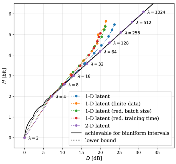
Figure 1: Circle: Entropy-Distortion tradeoff of ANN-based compressors with latent dimensions $1$ and $2$ along with lower bound and upper bound on optimal tradeoff.

III-B ANN Performance

To compress a source of dimension $d_{s}$ using a latent dimension of $d_{c}$, a stochastically-trained ANN-based compressor consists of an analysis transform $g_{a}:\mathbb{R}^{d_{s}}\mapsto\mathbb{R}^{d_{c}}$, a synthesis transform $g_{s}:\mathbb{R}^{d_{c}}\mapsto\mathbb{R}^{d_{s}}$, a quantizer and an entropy model that is factorized across each dimension of the codeword. The analysis and synthesis transforms are fully-connected feedforward neural networks with $2$ hidden layers containing $100$ neurons each. The quantization operation is not differentiable, and therefore during training we replace it with a differentiable proxy that varies over the course of the training process, beginning with dithered quantization and ending with the hard quantizer that is used at test time [9]. During training, a $d_{s}$-dimensional vector is fed into the analysis transform to obtain a $d_{c}$-dimensional latent vector. The quantization-proxy is then applied to the latent vector, which is then fed to the synthesis transform to obtain the $d_{s}$-dimensional reconstruction. The entropy model is a feedforward neural network that computes the entropy, $E$ of the quantized latents. Distortion $D$ is the mean-squared error between the reconstruction and the input vector. The Lagrangian $E+\lambda D$ is stochastically minimized over the trainable parameters of the ANN-based compressor using Adam [10]. We sweep across different values of $\lambda$ to obtain points on the lower convex hull of the ANN-compressor’s entropy-distortion tradeoff. We remark that the neural-network architecture and entropy model are similar to the ANN-based compressor trained for the sawbridge process in [5]. Since the circle is described by the scalar random variable $\theta$, we take the latent dimension $d_{c}=1$. The resulting performance is shown in Fig. 1. We see that the performance is suboptimal at high-SNR.

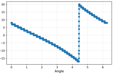
(a)

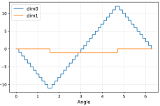
(b)

Figure 2: (a) Quantized encoder output vs. angle $\theta$ for $\lambda=512$ and $1$-D latent (away from optimal tradeoff). The analysis transform is not sufficiently steep. (c) Quantized encoder output vs. angle $\theta$ for $\lambda=512$ and $2$-D latents (on optimal tradeoff). 2-D latents are discussed in Section V.

To see why, note that intuition suggests, and the proofs of Theorems 3 and 4 essentially confirm, that an optimal scheme for compressing the circle is to quantize the angle $\theta$ into contiguous cells, all but (at most) one of which are the same size. Thus we would like the analysis transform to extract the angle $\theta$ from the realization of the circle, i.e., to implement $\mathrm{atan2({\overrightarrow{Z}})}$ or some scaled and shifted version thereof. The issue is that the function ${\overrightarrow{Z}}\mapsto\theta$ is not continuous over the circle, while the analysis transform must be continuous (and indeed differentiable) by construction.

This is confirmed in Fig. 2(a), which shows the quantized output of the trained analysis transform $g_{a}$ as a function of the angle $\theta$ at high SNR. We see that the analysis transform attempts to implement a discontinuity around 4.5 radians, but the function is insufficiently steep, so it passes through various intermediate quantization levels on its way from its minimum value to its maximum value. This creates an identifiability problem at the decoder, in that certain quantizer outputs can be caused by two values of $\theta$, one in the decreasing part of the function and one in the increasing part. Of course, the location of the discontinuity (4.5 radians in this case) is arbitrary and will be different if the network is retrained. At low SNR, the distortion accruing from this lack of invertibility is negligible compared to the distortion arising from the quantization process. At high rates, it dominates, and the performance is off the optimal entropy-distortion curve. The extent of the suboptimality is determined by how steep the analysis transform can be made, which in turn is controlled by the training process. In order for the training process to make the “steep” portion of the analysis transform steeper, we require source realizations from the range over which the function is steep to be present in the batch. Smaller batch sizes are less likely to include such points, and thus reducing the batch size leads to a larger gap from optimality (Fig. 1). Fixing a training data set (instead of drawing fresh samples at each iteration) has a similar effect, because once the steep portion of the function falls entirely between two training points, the training process has no incentive to make it steeper (Fig. 1). This issue is not unique to the circle in the Euclidean plane. Indeed, it can arise in more complex sources whose support has a circular structure, such as the ramp process to which we turn next.

IV The Ramp

Consider the following process.

$$J_{t}\stackrel{{\scriptstyle\text{def}}}{{=}}\left[\left(t+V\right)\text{ mod }1\right]-\frac{1}{2},$$ (19)

where $V\sim\text{Unif}\left[0,1\right]$. We call this the ramp process and $V$ the phase. We are interested in this process as a model of low-dimensional structure in high-dimensional spaces: on the one hand, the set of source realizations has infinite linear span; on the other hand, the realization is completely determined by the scalar random variable $V$. Note that $V=1$ and $V=0$ yield identical realizations of the ramp. Thus the set of realizations forms a circle in function space in some sense. This process is similar in some important respects to the “sawbridge” process considered in an earlier work [5]. But whereas the sawbridge is optimally compressed by the ANN-based architecture under study, we shall see that the ramp is not.

Since realizations of the ramp process are in one-to-one correspondence with realizations of $V$, it is natural to compress the ramp process by quantizing the $V$. The next theorem confirms that this is indeed optimal.

IV-A The Optimal Tradeoff

Theorem 5.

For the ramp, if $D\geq\frac{1}{12}$, $E_{\text{r}}(D)=0$. If $0<D<\frac{1}{12}$, then

$$E_{\text{r}}(D)=\inf\limits_{\left\{p_{i}\right\}_{i=1}^{\infty}}\quad- \sum\limits_{i=1}^{\infty}p_{i}\log p_{i}$$ (20)

s.t. $$\sum\limits_{i=1}^{\infty}\frac{p_{i}^{2}(2-p_{i})}{12}\leq D,$$ (21)

$$\sum\limits_{i=1}^{\infty}p_{i}=1,p_{i}\geq 0\text{ for all i}.$$ (22)

Proof.

Let $f_{\text{ramp}}:L^{2}\left[0,1\right]\mapsto\mathbb{N}$ be an encoder. Each value of the phase variable defines a unique realization. Therefore, define $S_{i}=f_{\text{ramp}}^{-1}\left(i\right)$ where

$$f_{\text{ramp}}^{-1}\left(i\right)\stackrel{{\scriptstyle\text{def}}}{{=}}\left\{v\in\left[0,1\right]:f_{\text{ramp}}\left([(t+v)\text{ mod}1]-0.5\right)=i\right\}.$$ (23)

Let $\mu$ be the Lebesgue measure. The optimal reconstruction is $t\mapsto\mathbb{E}\left[J_{t}\mid f_{\text{ramp}}(J_{t})\right]$. Thus the entropy and distortion of the encoder-decoder pair is given by

$$H\left(f_{\text{ramp}}\right) =-\sum_{i}\mu(S_{i})\log\left(\mu(S_{i})\right),$$

$$D\left(f_{\text{ramp}}\right) =\mathbb{E}\left[\int_{0}^{1}\left(J_{t}-\mathbb{E}\left[J_{t}\mid f_{\text{ramp}}(J_{t})\right]\right)^{2}dt\right].$$

The distortion can be expressed as

$$\mathbb{E}\left[\int_{0}^{1}\left(J_{t}-\mathbb{E}\left[J_{t}\mid f_{\text{ramp}}(J_{t})\right]\right)^{2}dt\right]$$ (24)

$$=\sum_{i}\mu\left(S_{i}\right)\mathbb{E}\left[\int_{0}^{1}\left(J_{t}-\mathbb{E}\left[J_{t}\mid V\in S_{i}\right]\right)^{2}dt\middle|V\in S_{i}\right]$$ (25)

$$=\sum_{i}\mu\left(S_{i}\right)\left(\mathbb{E}\left[\int_{0}^{1}J_{t}^{2}dt\mid V\in S_{i}\right]-\right.$$ (26)

$$\left.\hskip 113.81102pt\int_{0}^{1}\left(\mathbb{E}\left[J_{t}\middle|V\in S_{i}\right]\right)^{2}\;dt\right)$$ (27)

$$=\sum_{i}\mu\left(S_{i}\right)\left(\frac{1}{12}-\int_{0}^{1}\left(\mathbb{E}\left[J_{t}\mid V\in S_{i}\right]\right)^{2}dt\right).$$ (28)

where the last line follows because, irrespective of the phase, we have $\int_{0}^{1}J_{t}^{2}\;dt=\frac{1}{12}$.

We will show that, for any measurable $S\subset[0,1]$, we have

$$\int_{0}^{1}\left(\mathbb{E}\left[J_{t}\mid V\in S\right]\right)^{2}dt\leq\frac{1}{3}{\left({\frac{1-\mu{\left({S}\right)}}{2}}\right)}^{2}.$$ (29)

Write $y_{t}=E[J_{t}|V\in S]$. Then we have

$$\mathbb{E}\left[(t+V\mod 1)-\frac{1}{2}\middle|V\in S\right]$$ (30)

$$=\mathbb{E}\left[{\left({t+V-\frac{3}{2}}\right)}1(t+V>1)\right.$$

$$\hskip 14.22636pt+\left.{\left({t+V-\frac{1}{2}}\right)}1(t+V\leq 1)\middle|V\in S\right]$$

$$=t+\mathbb{E}[V|V\in S]-\mathbb{P}{\left({t+V>1\mid V\in S}\right)}-\frac{1}{2}$$

$$=t+\mathbb{E}[V|V\in S]-\frac{\mu{\left({S\cap[1-t,1]}\right)}}{\mu(S)}-\frac{1}{2}.$$ (31)

From (30) we see that the left-hand side of (29) is invariant with respect to cyclic rotation of $S$ of the form $S\mapsto s+S\mod 1$. Evidently the right-hand side of (29) is also invariant with respect to such a shift. Thus to show (29) we may cyclically rotate $S$ as convenient.

First, suppose that $S$ can be cyclicly rotated to obtain an interval of the form $[0,s]$. In this case (31) reads

$$y_{t}=\begin{cases}t\left(1-\frac{1}{s}\right)+\frac{s}{2}-\frac{3}{2}+\frac{1}{s}&\text{if $t>1-s$}\\ t-\frac{1-\mu{\left({S}\right)}}{2}&\text{if $t\leq 1-s$},\end{cases}$$ (32)

and thus we can explicitly compute

$$\int_{0}^{1}y_{t}^{2}dt=\frac{1}{3}{\left({\frac{1-\mu(S)}{2}}\right)}^{2}.$$ (33)

and equality in (29) holds in this case. More generally, suppose that $S$ is a finite union of closed, disjoint intervals, $S_{0},\ldots,S_{n-1}$ such that all points in $S_{0}$ are less than those in $S_{1}$, etc. Due to the rotational invariance of (29), we can assume that $\min S_{0}=0$ and $\max S_{n-1}<1$. Define

$$s_{i} =\min S_{i}\quad i=0,\ldots,n-1$$ (34)

$$s_{n} =1$$ (35)

$$t_{i} =s-s_{n-i}\quad i=0,\ldots,n.$$ (36)

Note that for each $i$, from (31), over the interval $[t_{i},t_{i+1}]$, $y_{t}$ is linearly increasing and then decreasing. Thus for $t\in[t_{i},t_{i+1}]$,

$$y_{t}\leq y_{t_{i}}+\frac{t-t_{i}}{t_{i+1}-t_{i}}(y_{t_{i+1}}-y_{t_{i}})$$ (37)

and as a result

$$\int_{t_{i}}^{t_{i+1}}y_{t}\;dt\leq\frac{y_{t_{i}}+y_{t_{i+1}}}{2}[t_{i+1}-t_{i}].$$ (38)

Since every realization of $J_{t}$ integrates to zero, we have

$$0 =\mathbb{E}\left[\int_{0}^{1}J_{t}dt\middle|V\in S\right]$$

$$=\int_{0}^{1}\mathbb{E}[J_{t}|V\in S]dt$$

$$=\int_{0}^{1}y_{t}dt$$

$$=\sum_{i=0}^{n-1}\int_{s_{i}}^{s_{i+1}}y_{t}dt$$

$$\leq\sum_{i=1}^{n}\frac{y_{t_{i}}+y_{t_{i+1}}}{2}\left[t_{i+1}-t_{i}\right].$$

It follows that there exists $i$ such that $y_{t_{i}}+y_{t_{i+1}}>0$. By rotational invariance, we can assume that $i=0$. Consider the modified set $\tilde{S}=\tilde{S}_{0}\cup\cdots\cup\tilde{S}_{n-1}$ wherein $\tilde{S}_{i}=S_{i}$ for $i=0,\ldots,n-2$ and $\tilde{S}_{n-1}$ is a closed interval satisfying $\mu(\tilde{S}_{n-1})=\mu(S_{n-1})$ and $\max\tilde{S}_{n-1}=1$. In words, we shift $S_{n-1}$ to the right so that its right end-point is 1. Define

$$\tilde{y}_{t}=\mathbb{E}[J_{t}|V\in\tilde{S}]$$ (39)

and note that, from (31), we have

$$\tilde{y}_{t}=\begin{cases}y_{0}+y_{t_{1}}-y_{t_{1}-t}&\text{if $t\in[0,t_{1}]$}\\ y_{t}&\text{if $t\in(t_{1},1]$}.\end{cases}$$ (40)

From this it follows that the norm of $\tilde{y}_{t}$ dominates that of $y_{t}$:

$$\int_{0}^{1}\tilde{y}_{t}^{2}dt =\int_{0}^{t_{1}}{\left({y_{0}+y_{t_{1}}-y_{t_{1}-t}}\right)}^{2}dt+\int_{t_{1}}^{1}y_{t}^{2}dt$$ (41)

$$=\int_{0}^{1}y_{t}^{2}dt+{\left({y_{0}+y_{t_{1}}}\right)}^{2}t_{1}$$ (42)

$$\hskip 14.22636pt-2(y_{0}+y_{t_{1}})\int_{0}^{t_{1}}y_{t}dt$$ (43)

$$\geq\int_{0}^{1}y_{t}^{2}dt,$$ (44)

where the final equality follows from (37) and the assumption that $y_{t_{i}}+y_{t_{i+1}}>0$. Now $\tilde{S}$ can be written as a union of $n-1$ disjoint closed intervals, since $\tilde{S}_{0}$ and $\tilde{S}_{n-1}$ are effectively conjoined. Repeating this process until we arrive at a single interval and then applying (33) gives

$$\int_{0}^{1}\mathbb{E}[J_{t}|V\in S]^{2}dt\leq\frac{1}{3}{\left({\frac{1-\mu(S)}{2}}\right)}^{2}$$ (45)

for any $S$ that is a disjoint union of closed intervals. Finally, consider an arbitrary (measurable) $S\subset[0,1]$. Then for any $\epsilon>0$, there exists a $\tilde{S}\subset[0,1]$ that is finite union of disjoint closed intervals such that

$$\mu{\left({(S\backslash\tilde{S})\cup(\tilde{S}\backslash S)}\right)}$$ (46)

can be made arbitrarily small [8, Theorem 1.20], and in particular for any $\epsilon$ we can have

$$\left|\frac{\mathbb{E}[V\cdot 1(V\in S)]}{\mathbb{P}(V\in S)}-\frac{\mathbb{E}[V\cdot 1(V\in\tilde{S})]}{\mathbb{P}(V\in\tilde{S})}\right| \leq\epsilon$$ (47)

$$\left|\frac{\mu(S\cap[1-t,1])}{\mu(S)}-\frac{\mu(\tilde{S}\cap[1-t,1])}{\mu(\tilde{S})}\right| \leq\epsilon.$$ (48)

Define the two conditional means

$$y_{t} =\mathbb{E}[J_{t}|V\in S]$$

$$\tilde{y}_{t} =\mathbb{E}[J_{t}|V\in\tilde{S}].$$

Then from (47) and (48) we have, for each $t$,

$$y_{t}\leq\tilde{y}_{t}+2\epsilon,$$

which, since

$$\int_{0}^{1}\tilde{y}_{t}dt=0.$$ (49)

implies that

$$\int_{0}^{1}y_{t}^{2}dt \leq\frac{1}{3}\left(\frac{1-\mu(\tilde{S})}{2}\right)^{2}+4\epsilon^{2}$$ (50)

$$\leq\frac{1}{3}\left(\frac{1-\mu(S)+\epsilon}{2}\right)^{2}+4\epsilon^{2},$$ (51)

from (48). Taking $\epsilon\rightarrow 0$ establishes (29).

Now given any code, $f_{\text{ramp}}$, for the ramp, define $S_{i}$ as in (23). Then we have from (28)

$$D\left(f_{\text{ramp}}\right) =\sum_{i}\mu(S_{i}){\left({\frac{1}{12}-\int_{0}^{1}\mathbb{E}[J_{t}|V\in S_{i}]^{2}dt}\right)}$$ (52)

$$\geq\sum_{i}\mu(S_{i}){\left({\frac{1}{12}-\frac{1}{3}\left(\frac{1-\mu(S_{i})}{2}\right)^{2}}\right)}$$ (53)

$$=\sum_{i}\mu(S_{i}){\left({\frac{1}{6}\mu(S_{i})-\frac{1}{12}\mu^{2}(S_{i})}\right)}.$$ (54)

Setting $p_{i}=\mu(S_{i})$ establishes the converse of the theorem. Achievability follows by noting that, for any $\{p_{i}\}$ satisfying the constraint in (21), we can create a code with entropy $-\sum_{i}p_{i}\log p_{i}$ satisfying the distortion constraint by setting $S_{0},S_{1},\ldots,S_{n-1}$ to be intervals with $\mu(S_{i})=p_{i}$ and noting equality in (29). ∎

The entropy-distortion function in (5) is formally an infinite-dimensional optimization problem. The following lower bound is easily computed.

Theorem 6.

$$E_{\text{r}}(D)\geq\sup\limits_{\lambda\geq 0}\inf_{0<p_{i}<1}-\log(p_{i})+\lambda\frac{p_{i}(2-p_{i})}{12}.$$ (55)

Proof.

By weak duality,

$$E_{\text{r}}(D) \geq\sup\limits_{\lambda\geq 0}\inf_{\begin{subarray}{c}\left\{p_{i}\right\}_{i=1}^{\infty}:\\ \sum_{i}p_{i}=1,\\ p_{i}\geq 0\text{ for all }i\end{subarray}}\sum\limits_{i=1}^{\infty}-p_{i}\log(p_{i})+\lambda\frac{p_{i}^{2}(2-p_{i})}{12}$$

$$=\sup\limits_{\lambda\geq 0}\inf_{\begin{subarray}{c}\left\{p_{i}\right\}_{i=1}^{\infty}:\\ \sum_{i}p_{i}=1,\\ p_{i}\geq 0\text{ for all }i\end{subarray}}\sum\limits_{i=1}^{\infty}p_{i}{\left({-\log(p_{i})+\lambda\frac{p_{i}(2-p_{i})}{12}}\right)}$$

$$\geq\sup\limits_{\lambda\geq 0}\inf_{0<p_{i}<1}-\log(p_{i})+\lambda\frac{p_{i}(2-p_{i})}{12}.$$

∎

The bound in Theorem 55 is illustrated in Fig. 3 (“lower bound”). For rates equal to $\log K$ where $K\geq 2$ is an integer, an achievable scheme uniformly quantizes the phase. The encoder assigns a ramp realization $J_{t}$ to the midpoint of the interval that contains $J_{0}+0.5$. The decoder outputs the conditional mean of the ramp restricted to the phase lying in the encoded interval. For rates between $\log K$ and $\log K+1$, an upper bound on the optimal tradeoff is obtained by dividing the ramp into biuniform intervals, where one interval has length $\varepsilon$ and the other $K$ intervals have length $\frac{1-\varepsilon}{K}$.

We next compare this optimal performance against that of stochastically-trained ANN-based compressors.

IV-B ANN performance

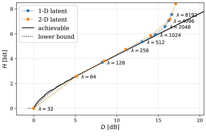
Figure 3: Entropy-distortion tradeoff for ramp.

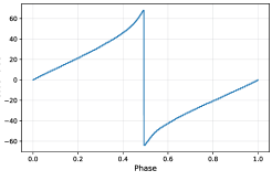
(a)

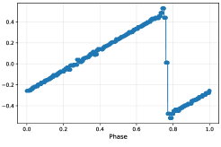
(b)

Figure 4: (a) Quantized encoder output vs. phase for $\lambda=4096$ (away from optimal tradeoff). (b) Reconstruction at randomly chosen index vs. phase for $\lambda=4096$. Here the synthesis transform is insufficiently steep.

Figure 3 shows the entropy-distortion tradeoff for the ANN-based compressor. We see that the performance is suboptimal at high rates. The problem is similar to that which arose with the circle. Per Theorem 5, we expect the analysis transform to output the phase $V$, or some scaled and shifted version of it such as $Y=\alpha(v+V\mod 1)+\beta$. The training process does indeed find such a solution for $g_{a}(\cdot)$, as shown in Fig. 4(a). Now consider the synthesis transform, $g_{s}(\cdot)$, evaluated at a particular output time, $t$. The mapping we require in order to recover $J_{t}$ from $Y$ is

$$Y\mapsto((Y-\beta)/\alpha+t-v)\mod 1.$$ (56)

This function is not continuous, however, and being a multilayer perceptron, $g_{s}(\cdot)$ must be continuous (and indeed differentiable). In practice, the trained synthesis transform will implement a continuous approximation to (56) that incurs distortion because its discontinuity is insufficiently steep. The situation is thus analogous to the circle. Note that for the circle, however, the problem arose with the analysis transform, whereas here it arises in the synthesis transform. Indeed, evaluating the ramp at one fixed time $t$ already has the desired form for the analysis transform,

$$J_{t}=\left[\left(t+V\right)\text{ mod }1\right]-\frac{1}{2}.$$ (57)

Thus the analysis transform can simply transmit any of the input samples directly, which is clearly a continuous map. On the other hand, Fig. 4(b) shows the reconstruction, evaluated at a fixed time index, as a function of $V$. We see that the discontinuity is insufficiently steep.

As with the circle, at low rates, the approximation error noted above is negligible compared with the quantization error, and thus this phenomenon does not lead to entropy-distortion suboptimality.

V Overparametrizing the Latent Space

One possible workaround to the suboptimality identified above is to overparametrize the latent space. In the above examples, the analysis transform could output a 2-D vector ($d_{c}=2$) rather than a scalar, for instance. In the case of the circle, this evidently solves the identifiability problem, as the analysis transform can now simply be the identity map. This makes the quantization problem more difficult, however, because the latent variables are always quantized independently of each other, but if the analysis transform is indeed the identity map then the two latent variables are not statistically independent (though they are uncorrelated). With an identity analysis transform, it is possible to independently quantize the two latent variables so that the overall system is optimal if one uses quantizers that are highly asymmetrical between the two components. Specifically, one of the components is quantized to a single bit to indicate which hemisphere the source is in, and the other is quantized with high resolution. The resulting system will be optimal so long as the quantized values are independent and uniformly distributed over their respective supports. Remarkably, with enough training, the network is able to find this solution, as shown in Figs. 1 and 2(b). Of course, this only works when the number of reconstructions is even.

For the ramp, on the other hand, overparametrizing the latent space appears to provide little benefit (Fig. 3). From the discussion in Section IV, this is unsurprising.

VI Discussion

We conclude that the argument that ANN-based compressors are adept at compressing low-dimensional manifolds should be applied with some care. While ANNs are essentially optimal compressors for some manifolds [5], they are suboptimal for the sources exhibiting a circular topology considered in this paper.

Low-level models of natural images have long included spatially-local image features that exist on one or more intrinsic dimensions and can be organized on circular topologies, such as spatial orientation [11, 12, 13, 14]. It has also been noted that different edge or feature profiles can be determined by their phase, another dimension which has a circular topology, and their phase congruency, in complex wavelet representations [15, 16]. Empirically, it has been shown that local image statistics are inherently low-dimensional [17] and that these local statistics live on a topology equivalent to a Klein bottle [18], a topology which is also found in orientation-selective complex wavelet filters. Thus while the sources considered in this paper are obviously synthetic, the findings in this paper may have some applicability to image compression.

Beyond the findings about ANN-based compressors, we have also determined the entropy-distortion functions of the circle and ramp. Classical rate-distortion theory has favored the study of Gaussian sources over those with low-dimensional manifold structure, despite the relevance of the latter to the study of image compression. Prior work on compression of low-dimensional sets includes rate-distortion tradeoffs for fractal sources [19] and rate-distortion analysis of compressed sensing [20, 21] More connected to the results of this paper, [22] provides a lower bound and [23] an upper bound on the rate-distortion function of the circle. We have provided a complete characterization of the entropy-distortion function.

References

• [1] Johannes Ballé, Valero Laparra and Eero P Simoncelli “End-to-end Optimized Image Compression” In International Conference on Learning Representations, ICLR 2017, 2017
• [2] Johannes Ballé et al. “Variational image compression with a scale hyperprior” In International Conference on Learning Representations, ICLR 2018, 2018
• [3] Fabian Mentzer, George Toderici, Michael Tschannen and Eirikur Agustsson “High Fidelity Generative Image Compression” In Advances in Neural Information Processing Systems 34, 2020
• [4] Johannes Ballé et al. “Nonlinear Transform Coding” In IEEE Journal of Selected Topics in Signal Processing 15.2 IEEE, 2020, pp. 339–353
• [5] A.. Wagner and Johannes Ballé “Neural Networks Optimally Compress the Sawbridge” arXiv:2011.05065
• [6] James R Munkres “Topology” Prentice Hall Upper Saddle River, 2000
• [7] Thomas M. Cover and Joy A. Thomas “Elements of Information Theory” Hoboken: John Wiley & Sons, 2006
• [8] Gerald B. “Real Analysis” Wiley Interscience, 1999
• [9] Eirikur Agustsson and Lucas Theis “Universally Quantized Neural Compression” In Advances in Neural Information Processing Systems 33, 2020, pp. 12367–12376
• [10] D.P. Kingma, Jimmy Ba, Yoshua Bengio and Yann LeCun “Adam: A method for stochastic optimization” In 3rd International Conference on Learning Representations, 2015
• [11] Eero P. Simoncelli, William T. Freeman, Edward H. Adelson and David J. Heeger “Shiftable Multiscale Transforms” In IEEE Trans. on Information Theory 38.2, 1992 DOI: 10.1109/18.119725
• [12] Bruno Olshausen and David J. Field “Emergence of Simple-Cell Receptive Field Properties by Learning a Sparse Code for Natural Images” In Nature 381, 1996 DOI: 10.1038/381607a0
• [13] Anthony J. Bell and Terrence J. Sejnowski “The “Independent Components” of Natural Scenes are Edge Filters” In Vision Research 37.23, 1997 DOI: 10.1016/S0042-6989(97)00121-1
• [14] J.. Hateren and A. Schaaf “Independent Component Filters of Natural Images Compared with Simple Cells in Primary Visual Cortex” In Proc. of the Royal Society of London B: Biological Sciences 265.1394, 1998 DOI: 10.1098/rspb.1998.0303
• [15] Svetha Venkatesh and Robyn A. Owens “On the Classification of Image Features” In Pattern Recognition Letters 11.5, 1990, pp. 339–349 DOI: 10.1016/0167-8655(90)90043-2
• [16] Peter Kovesi “Image Features from Phase Congruency” In Videre: Journal of Computer Vision Research 1.3, 1999, pp. 2–26
• [17] Olivier Hénaff, Johannes Ballé, Neil C. Rabinowitz and Eero P. Simoncelli “The Local Low-Dimensionality of Natural Images” In 3rd Int. Conf. on Learning Representations (ICLR), 2015 arXiv:1412.6626
• [18] Gunnar Carlsson, Tigran Ishkhanov, Vin Silva and Afra Zomorodian “On the Local Behavior of Spaces of Natural Images” In Int. Journal of Computer Vision 76, 2008 DOI: 10.1007/s11263-007-0056-x
• [19] Tsutomu Kawabata and Amir Dembo “The Rate-distortion Dimension of Sets and Measures” In IEEE Transactions on Information Theory 40.5 IEEE, 1994, pp. 1564–1572
• [20] Yihong Wu and Sergio Verdú “Rényi Information Dimension: Fundamental Limits of Almost Lossless Analog Compression” In IEEE Transactions on Information Theory 56.8, 2010, pp. 3721–3748 DOI: 10.1109/TIT.2010.2050803
• [21] Markus Leinonen, Marian Codreanu, Markku Juntti and Gerhard Kramer “Rate-Distortion Performance of Lossy Compressed Sensing of Sparse Sources” In IEEE Transactions on Communications 66.10, 2018, pp. 4498–4512 DOI: 10.1109/TCOMM.2018.2834349
• [22] Erwin Riegler, Helmut Bölcskei and Günther Koliander “Rate-distortion Theory for General Sets and Measures” In 2018 IEEE International Symposium on Information Theory (ISIT), 2018, pp. 101–105 IEEE
• [23] Günther Koliander, Georg Pichler, Erwin Riegler and Franz Hlawatsch “Entropy and Source Coding for Integer-dimensional Singular Random Variables” In IEEE Transactions on Information Theory 62.11 IEEE, 2016, pp. 6124–6154