Entanglement harvesting between two inertial Unruh-DeWitt detectors from non-vacuum quantum fluctuations

Abstract

Entanglement harvesting from the quantum field is a well-known fact that, in recent times, is being rigorously investigated further in flat and different curved backgrounds. The usually understood formulation studies the possibility of two uncorrelated Unruh-DeWitt detectors getting entangled over time due to the effects of quantum vacuum fluctuations. Our current work presents a thorough formulation to realize the entanglement harvesting from non-vacuum background fluctuations. In particular, we further consider single excitation field states and a pair of inertial detectors, respectively, in $(1+1)$ and $(1+3)$ dimensions for this investigation. Our main observation asserts that entanglement harvesting is suppressed compared to the vacuum fluctuations in this situation. Our other observations confirm a non-zero individual detector transition probability in this background and vanishing entanglement harvesting for parallel co-moving detectors. We look into the characteristics of the harvested entanglement and discuss its dependence on different system parameters.

I Introduction

The investigations to understand quantum entanglement-related phenomena for relativistic particles have gained significant momentum recently (see Fuentes-Schuller and Mann (2005); Reznik (2003); Lin and Hu (2010); Ball et al. (2006); Cliche and Kempf (2010); Martin-Martinez and Menicucci (2012); Salton et al. (2015); Martin-Martinez et al. (2016); Cai and Ren (2018); Menezes (2018); Menezes et al. (2017); Zhou and Yu (2017); Benatti and Floreanini (2004); Pan and Zhang (2020); Barman and Majhi (2021); Kane and Majhi (2021); Barman and Majhi (2022); Barman et al. (2022)). This veneration of quantum entanglement lies in its fascinating nature to be able to distinguish a quantum phenomenon from a classical one. Furthermore, the discovery of gravitational waves provided additional interest in this direction. Though predicted entirely from the classical considerations, these discoveries encourage one to look also for the signatures of the quantum phenomena from the early universe. Therefore, entanglement is revered as an arena to broaden our conceptual horizon, and it is also relevant from many practical fronts. In particular, it finds its applications in many forerunning expectations of modern technology like quantum communication, cryptography, and teleportation Tittel et al. (1998); Sal . The experimental verification of entanglement in systems with photons and even in electrons Kirby and Franson (2013); Hensen et al. (2015) makes these possibilities all the more lucrative. In this regard, an enormous amount of interest is given to the possibility of two initially uncorrelated systems getting entangled over time, which is better known in the literature as the entanglement harvesting. It predicts that from the vacuum fluctuation of the quantum fields, depending upon the motions of the systems, one can harvest entanglement between two or more systems when they are interacting with the background quantum fields. Moreover, one can further utilize this for quantum information-related works like quantum teleportation Hotta (2008, 2009); Frey et al. (2014). The works Valentini (1991); Reznik (2003); Reznik et al. (2005); Salton et al. (2015) first introduced the idea of entanglement harvesting. In particular, the work Reznik (2003), where Reznik pioneered this phenomenon, considers point-like two-level Unruh-DeWitt (UD) hypothetical particle detectors. In this work, the author provided the understanding of entanglement harvesting between two accelerated and causally disconnected UD detectors (initially conceptualized to understand the Unruh effect Unruh (1976); Unruh and Wald (1984)), which interact with the background massless scalar field. Since these articles, there has been a significant amount of research towards the realization of entanglement harvesting from the quantum field vacuum in different spacetime backgrounds as well as for various types of motions of detectors Martín-Martínez et al. (2013); Lorek et al. (2014); Ver Steeg and Menicucci (2009); Brown et al. (2014); Pozas-Kerstjens and Martin-Martinez (2015, 2016); Martin-Martinez et al. (2016); Kukita and Nambu (2017); Sachs et al. (2017); Trevison et al. (2019); Li et al. (2018); Henderson et al. (2018); Henderson and Menicucci (2020); Stritzelberger et al. (2020); Koga et al. (2018); Ng et al. (2018); Koga et al. (2019); Brown (2013); Simidzija and Martín-Martínez (2018); Lima et al. (2020); Barman et al. (2021a, b). Also the relative motion of the detectors has significant impact on the initial entanglement between them Chowdhury and Majhi (2022). However, there remain many other extensive areas to venture further in this endeavour. One such area is the possibility of entanglement harvesting from the non-vacuum quantum fluctuations, which may be relevant from the practical point of view. Till now, so far we are aware of, no investigation related to entanglement harvesting with the excited fields has been done. This venture gains its motivation as, in nature, it is not guaranteed that the background field will be in a vacuum state. And if the background field state is indeed in some excited state, how much do the results concerning the entanglement harvesting change compared to the vacuum fluctuations.

In the current work, we are going to investigate the entanglement harvesting condition (see Koga et al. (2018, 2019); Hu and Yu (2015) for elaborate discussions on these conditions), for two UD detectors in inertial motion interacting with the single-particle background field states (motivated from the work Lochan and Padmanabhan (2015) where the detector’s response function for an accelerated detector in single particle excited state has been studied) in $(1+1)$ and $(1+3)$ dimensions. In principle the field can be in any excited state; but here, following Lochan and Padmanabhan (2015), we consider the simplest model where the fields are in single-particle excited state. We will see that this becomes an analytically tractable system. In particular, we have considered detectors in parallel inertial motion in $(1+1)$ dimensions, and in parallel and perpendicular inertial motions in $(1+3)$ dimensions. Our study involves detectors interacting for eternity with the background massless, minimally coupled scalar quantum field through monopole-type couplings. Here we aim to provide a rigorous formulation for entanglement harvesting with a background non-vacuum field state. In this regard, we have followed the works Koga et al. (2018, 2019), where one can thoroughly understand entanglement harvesting conditions with detectors interacting with the field vacuum.

In particular, our principal observation in this work is that the entanglement harvested with inertial detectors from the single-particle field states is lower than that harvested from the field vacuum. In this regard, we consider normalizable single-particle states with two specific types of distribution functions. Namely the exponential decaying and the Gaussian distribution functions (see Lochan and Padmanabhan (2015) for elaborate discussions on these field states). We also observe that in both $(1+1)$ and $(1+3)$ dimensions, inertial UD detectors’ self transition probabilities are non-zero due to the non-vacuum background fluctuations. In $(1+1)$ dimensions, our observations suggest that one cannot harvest entanglement between two comoving inertial detectors. In $(1+3)$ dimensions, two parallelly moving observers with equal velocity do not harvest entanglement. While in perpendicular motion, we do not confirm a similar situation. Furthermore, in this work, we elucidate the different characteristics of entanglement harvesting and study its dependence on the parameters of our considered system.

This work is organized as follows. In sec. II we shall provide a brief discussion of the model set-up consisting of two UD detectors interacting with a minimally coupled, massless scalar field through monopole couplings in the background of a non-vacuum field state. This section contains the discussion on the general mathematical description of the entanglement harvesting condition. In sec. III we shall consider two inertial Unruh-DeWitt detectors in $(1+1)$ dimensions and investigate the individual detector transition probabilities and entanglement harvesting conditions. Subsequently, in sec. IV, UD detectors are considered in $(1+3)$ dimensions for studying the same relevant quantities. There are two special cases for $(1+3)$ dimensions; one is for parallel motion, and the other is for the perpendicular motion of the detectors. They constitute different subsections. We conclude by discussing our findings in sec. V.

II The model and working formulas

This section presents the formulation for understanding the possibility of two uncorrelated atomic Unruh-DeWitt detectors getting entangled over time while interacting with a general field state. Particularly we are interested to find the condition to be entangled and also the quantification of it will be done. The whole analysis will be valid till the second order perturbative series of the density matrix of the system, when the expansion is done order by order in terms of interaction strength.

II.1 The system: a general framework

We consider two two-level Unruh-DeWitt detectors, associated with our observers Alice and Bob, denoted as $A$ and $B$. Furthermore, we perceive the detectors to be point-like and interacting with a background massless, minimally coupled real scalar quantum field $\phi(X)$ through monopole interaction. Then the interaction action is given by

$$S_{int} = c\int_{-\infty}^{\infty}\left[\kappa_{A}\left(\tau_{A}\right)m_{A}\left(\tau_{A}\right)\Phi\left(X_{A}\left(\tau_{A}\right)\right)d\tau_{A}\right.$$ (1)

$$\left.~{}~{}~{}+\kappa_{B}\left(\tau_{B}\right)m_{B}\left(\tau_{B}\right)\Phi\left(X_{B}\left(\tau_{B}\right)\right)d\tau_{B}\right]\,,$$

where $c$ is the coupling constant between different detectors and the scalar field (which we have assumed to be the same for both the detectors $c_{A}=c_{B}=c$), $\kappa_{j}\left(\tau_{j}\right)$ is the switching function for $j^{th}$ detectors (with $j=A,~{}B$) and $\tau_{j}$ is the individual detector’s proper time. The initial state of the composite system is taken to be $|in\rangle=|\Psi\rangle|E_{0}^{A}\rangle|E_{0}^{B}\rangle$, where $|\Psi\rangle$ is a general field state and $|E_{n}^{j}\rangle$ is the $n^{th}$ state of detector $j~{}(n=0,1)$. In the asymptotic future one can obtain the final state of the system as $|out\rangle=T\{e^{iS_{int}}\}|in\rangle$. Then by tracing out the field degrees of freedom from the final total density matrix one can get the reduced density matrix for the detectors $\rho_{AB}$, which in the basis of $\{|E_{1}^{A}\rangle|E_{1}^{B}\rangle,|E_{1}^{A}\rangle|E_{0}^{B}\rangle,|E_{0}^{A}\rangle|E_{1}^{B}\rangle,|E_{0}^{A}\rangle|E_{0}^{B}\rangle\}$ is expressed as

$$\rho_{AB}=\begin{pmatrix}0&0&0&c^{2}\mathcal{E}\\ 0&c^{2}\mathcal{P}_{A}&c^{2}\mathcal{P}_{AB}&0\\ 0&c^{2}\mathcal{P}^{\star}_{AB}&c^{2}\mathcal{P}_{B}&0\\ c^{2}\mathcal{E}^{\star}&0&0&1-c^{2}\mathcal{P}_{A}-c^{2}\mathcal{P}_{B}\end{pmatrix}+O(c^{4}).$$ (2)

To arrive at this density matrix we have used the expression of the monopole moment operator $m_{j}(0)=|E_{0}^{j}\rangle\langle E_{1}^{j}|+|E_{1}^{j}\rangle\langle E_{0}^{j}|$. The expressions for the matrix elements are

$$\mathcal{P}_{j} = \left|\left\langle E_{1}^{j}\left|m_{j}(0)\right|E_{0}^{j}\right\rangle\right|^{2}\mathcal{I}_{j}\,,$$

$$\mathcal{E} = \left\langle E_{1}^{B}\left|m_{B}(0)\right|E_{0}^{B}\right\rangle\left\langle E_{1}^{A}\left|m_{A}(0)\right|E_{0}^{A}\right\rangle\mathcal{I}_{\varepsilon}\,,$$

$$\mathcal{P}_{AB} = \left\langle E_{1}^{A}\left|m_{A}(0)\right|E_{0}^{A}\right\rangle\left\langle E_{1}^{B}\left|m_{B}(0)\right|E_{0}^{B}\right\rangle^{\dagger}\mathcal{I}_{AB}\,.$$ (3)

Again the quantities $\mathcal{I}_{j}$, $\mathcal{I}_{AB}$ and $\mathcal{I}_{\varepsilon}$ in these expressions are given by

$$\mathcal{I}_{j} = \int_{-\infty}^{\infty}\int_{-\infty}^{\infty}{d\tau_{j}d\tau^{\prime}_{j}}\kappa_{j}(\tau_{j})\kappa_{j}(\tau^{\prime}_{j})e^{-i\Delta{E}(\tau_{j}-\tau^{\prime}_{j})}$$

$$~{}~{}~{}~{}~{}~{}~{}~{}~{}~{}~{}~{}~{}~{}~{}~{}~{}~{}~{}~{}~{}~{}~{}~{}~{}~{}\times\langle\Psi|\phi(X_{j})\phi(X^{\prime}_{j})|\Psi\rangle\,,$$

$$\mathcal{I}_{\varepsilon} = -\int_{-\infty}^{\infty}\int_{-\infty}^{\infty}{d\tau_{B}d\tau^{\prime}_{A}}\kappa_{B}(\tau_{B})\kappa(\tau^{\prime}_{A})e^{i\Delta{E}(\tau^{\prime}_{A}+\tau_{B})}$$

$$~{}~{}~{}~{}~{}~{}~{}~{}~{}~{}~{}~{}~{}~{}~{}~{}~{}~{}~{}~{}~{}~{}~{}\times\langle\Psi|T\phi(X_{B})\phi(X^{\prime}_{A})|\Psi\rangle\,,$$

$$\mathcal{I}_{AB} = \int_{-\infty}^{\infty}\int_{-\infty}^{\infty}{d\tau_{B}d\tau^{\prime}_{A}}\kappa_{B}(\tau_{B})\kappa_{A}(\tau^{\prime}_{A})e^{i\Delta{E}(\tau^{\prime}_{A}-\tau_{B})}$$ (4)

$$~{}~{}~{}~{}~{}~{}~{}~{}~{}~{}~{}~{}~{}~{}~{}~{}~{}~{}~{}~{}~{}~{}~{}~{}~{}~{}\times\langle\Psi|\phi(X_{B})\phi(X^{\prime}_{A})|\Psi\rangle\,,$$

where, $\langle\Psi|\phi(X_{i})\phi(X^{\prime}_{j})|\Psi\rangle$ is the two point function corresponding to a general field state. We should also mention that to arrive at these expressions the explicit forms of the initial field state $|\Psi\rangle$ were not needed, which is evident from Eq. (II.1). Mostly the expressions of the time evolution operators were exploited up to this point. In this regard, one may note that by replacing $|\Psi\rangle$ by the vacuum state $|0\rangle$, one can get the density matrix if the detectors were interacting with the fields in vacuum (or no particle state). Nevertheless, one may look into the article Koga et al. (2018) for a detailed understanding of the procedure to obtain these expressions in an initial field vacuum. The same method has been adopted here as well and we landed up a result which is in identical form as obtained for vacuum state; except the vacuum state has been replaced by a general excited field state in the correlation functions. Therefore the general discussion regarding the entanglement harvesting condition as well as measurement of harvested entanglement will exactly follow from previous literature, except the explicit measures of the quantities appearing in matrix elements will differ. The condition for the two detectors to get entangled Peres (1996); Horodecki et al. (1996), is obtained when the partial transposition of the reduced density matrix from Eq. (2) has negative eigenvalue. This condition is expressed as

$$\mathcal{P}_{A}\,\mathcal{P}_{B}<|\mathcal{E}|^{2}~{},$$ (5)

which can also be cast into the form Koga et al. (2018, 2019)

$$\mathcal{I}_{A}\mathcal{I}_{B}<|\mathcal{I}_{\varepsilon}|^{2}~{}.$$ (6)

Once the possibility of entanglement harvesting is arisen (i.e. the condition (6) is satisfied), one may study different entanglement measures to quantify the harvested entanglement. In this regard, in the two qubits case one of the convenient entanglement measures is the concurrence $\mathcal{C}(\rho_{AB})$ (see Koga et al. (2018, 2019); Hu and Yu (2015)), which enables one to estimate the entanglement of formation $E_{F}(\rho_{AB})$ (see Bennett et al. (1996); Hill and Wootters (1997); Wootters (1998); Koga et al. (2018, 2019)). For two-qubits system the concurrence Koga et al. (2018) is

$$\mathcal{C}(\rho_{AB}) = 2c^{2}\left(|\mathcal{E}|-\sqrt{\mathcal{P}_{A}\mathcal{P}_{B}}\right)+\mathcal{O}(c^{4})$$

$$= 2c^{2}|\langle E_{1}^{B}|m_{B}(0)|E_{0}^{B}\rangle||\langle E_{1}^{A}|m_{A}(0)|E_{0}^{A}\rangle|$$

$$~{}~{}~{}~{}~{}~{}\times\left(|\mathcal{I}_{\varepsilon}|-\sqrt{\mathcal{I}_{A}\mathcal{I}_{B}}\right)+\mathcal{O}(c^{4})~{}.$$ (7)

One can notice that the quantities $|\langle E_{1}^{j}|m_{j}(0)|E_{0}^{j}\rangle|$ are completely dependent on the detectors’ internal structure. The considered background spacetime, scalar fields, and the motions of the detectors do not contribute in them. Then from the point of view of investigating the entanglement harvesting due to the background spacetime and motions of detectors with specific configuration, it seems sufficient to study the nature of

$$\mathcal{C}_{\mathcal{I}}=\left(|\mathcal{I}_{\varepsilon}|-\sqrt{\mathcal{I}_{A}\mathcal{I}_{B}}\right)$$ (8)

in order to understand more about concurrence. We shall indeed be studying this quantity $\mathcal{C}_{\mathcal{I}}$ to understand the characteristics of entanglement harvesting in our considered system with respect to different parameters.

II.2 Choice of field state

We are interested on excited states of field and so in principle $|\Psi\rangle$ can be chosen as any excited field state or combination of all field states. For simplicity of calculation and analysis, in this study, we will consider $|\Psi\rangle$ to be consisted of only single exited field states corresponding to modes $u_{k}$. Such choice is mainly inspired from Lochan and Padmanabhan (2015) where the detector’s response function for its accelerated motion has been investigated. In $(1+d)$-dimensions, it can be expressed as Lochan and Padmanabhan (2015)

$$|\Psi\rangle=\int\frac{d^{d}k}{(2\pi)^{d/2}\sqrt{2\omega_{k}}}f(k)\hat{a}_{k}|0_{u}\rangle~{}.$$ (9)

where $\omega_{k}=|k|$ and $f(k)$ denotes the normalised probability amplitude of the distribution, which satisfies the normalization condition

$$\int\frac{d^{d}k}{(2\pi)^{d}{2\omega_{k}}}\left|f(k)\right|^{2}=1~{}.$$ (10)

In a singly excited state the two point function (for explicit derivation, see Birrell and Davies (1984); Lochan and Padmanabhan (2015)) is given as

$$\langle\Psi|\Phi(X_{j})\Phi(X^{\prime}_{j})|\Psi\rangle = G_{W}\left(X_{j},X^{\prime}_{j}\right)+\Phi_{{eff}}(X_{j})\Phi_{{eff}}^{\star}(X^{\prime}_{j})$$ (11)

$$~{}~{}~{}~{}~{}~{}+\Phi_{{eff}}^{\star}(X_{j})\Phi_{{eff}}(X^{\prime}_{j})\,,$$

where $G_{W}\left(X_{j},X^{\prime}_{j}\right)\equiv\langle 0_{u}|\Phi\left(X_{j}\right)\Phi\left(X^{\prime}_{j}\right)|0_{u}\rangle$ denote the positive frequency Wightman function with $T_{j}>T_{j^{\prime}}$. Moreover, $\Phi_{eff}$ is called the effective field, defined by Lochan and Padmanabhan (2015)

$$\Phi_{eff}(X_{j})=\int\frac{d^{d}k}{(2\pi)^{d}2\omega_{k}}f(k)e^{ik\cdot X_{j}}.$$ (12)

Now because of the fact that $f(k)$ is a scalar distribution it is convenient to consider $f(k)\equiv f(\omega_{k})$. With this line of thought, one may express the time ordered field expectation value as

$$\langle\Psi|T\,\phi(X_{j})\phi(X^{\prime}_{j})|\Psi\rangle = \theta(T_{j}-T^{\prime}_{j})\,\langle\Psi|\phi(X_{j})\phi(X^{\prime}_{j})|\Psi\rangle$$

$$~{}+\,\theta(T^{\prime}_{j}-T_{j})\,\langle\Psi|\phi(X^{\prime}_{j})\phi(X_{j})|\Psi\rangle$$ (13)

$$= i\,G_{F}\left(X_{j},X^{\prime}_{j}\right)+\Phi_{{eff}}(X_{j})\Phi_{{eff}}^{\star}(X^{\prime}_{j})$$

$$~{}~{}~{}~{}~{}~{}+\Phi_{{eff}}^{\star}(X_{j})\Phi_{{eff}}(X^{\prime}_{j})~{},$$

where, $\theta(T_{j}-T^{\prime}_{j})$ denotes the Heaviside step function, and we have used the expression of Eq. (11) to arrive at the last form. One should also note that here $G_{F}\left(X_{j},X^{\prime}_{j}\right)\equiv-i\langle 0_{u}|T\,\Phi\left(X_{j}\right)\Phi\left(X_{j^{\prime}}\right)|0_{u}\rangle$ denotes the Feynman propagator. Thus one can easily observe that the expressions given in (II.1) will contain two contributions – one from pure vacuum fluctuations and another part is due to the effect of choosing non-vacuum state. Therefore the entanglement harvesting phenomenon in this case effectively driven by vacuum fluctuation of the fields as well as by an effective field configuration emerged due to the non-vacuum property of field state. Hence we expect that the usual entanglement harvesting phenomenon through vacuum fluctuation suffers modification if the background field is in excited state.

Then one may also express the integral $\mathcal{I}_{\varepsilon}$ from Eq. (II.1) as

$$\mathcal{I}_{\varepsilon}=\mathcal{I}_{\varepsilon}^{vac}+\mathcal{I}_{\varepsilon}^{nv}~{},$$ (14)

where

$$\mathcal{I}_{\varepsilon}^{vac} = -i\int_{-\infty}^{\infty}\int_{-\infty}^{\infty}{d\tau_{B}d\tau^{\prime}_{A}}\,e^{i\Delta{E}(\tau^{\prime}_{A}+\tau_{B})}$$ (15a)

$$~{}~{}~{}~{}~{}~{}~{}~{}~{}~{}~{}~{}~{}~{}~{}~{}~{}~{}~{}\times G_{F}(X_{B},X^{\prime}_{A})~{},$$

$$\mathcal{I}_{\varepsilon}^{nv} = -\int_{-\infty}^{\infty}\int_{-\infty}^{\infty}{d\tau_{B}d\tau^{\prime}_{A}}\,e^{i\Delta{E}(\tau^{\prime}_{A}+\tau_{B})}$$

$$\times\,[\Phi_{{eff}}(X_{B})\Phi_{{eff}}^{\star}(X^{\prime}_{A})$$ (15b)

$$~{}~{}~{}~{}~{}~{}+\Phi_{{eff}}^{\star}(X_{B})\Phi_{{eff}}(X^{\prime}_{A})]~{}.$$

Here we have considered trivial switching functions $\kappa_{j}\left(\tau_{j}\right)=1$, which signifies that the detectors are eternally interacting with the field . Furthermore, using the relation between Feynman propagator and the Wightman function $iG_{F}\left(X,X^{\prime}\right)=G_{W}\left(X,X^{\prime}\right)+iG_{R}\left(X^{\prime},X\right)=G_{W}\left(X,X^{\prime}\right)+\theta(T^{\prime}-T)\left\{G_{W}\left(X^{\prime},X\right)-G_{W}\left(X,X^{\prime}\right)\right\}$ one can simplify the calculation of the integral $\mathcal{I}_{\varepsilon}^{vac}$ as

$$\mathcal{I}_{\varepsilon}^{vac} = \mathcal{I}_{\varepsilon_{W}}^{vac}+\mathcal{I}_{\varepsilon_{R}}^{vac},$$ (16)

with

$$\mathcal{I}_{\varepsilon_{W}}^{vac} = -\int_{-\infty}^{\infty}d\tau_{B}\int_{-\infty}^{\infty}d\tau_{A}~{}\scalebox{0.91}{$e^{i(\Delta E^{B}\tau_{B}+\Delta E^{A}\tau_{A})}$}$$

$$~{}~{}~{}~{}~{}~{}~{}~{}~{}~{}~{}~{}~{}~{}~{}~{}~{}\times\,G_{W}(X_{B},X_{A})\,,$$ (17a)

$$\mathcal{I}_{\varepsilon_{R}}^{vac} = -\int_{-\infty}^{\infty}d\tau_{B}\int_{-\infty}^{\infty}d\tau_{A}~{}\scalebox{0.91}{$e^{i(\Delta E^{B}\tau_{B}+\Delta E^{A}\tau_{A})}$}\theta(T_{A}-T_{B})$$

$$~{}~{}~{}\times\,\big{\{}G_{W}\left(X_{A},X_{B}\right)-G_{W}\left(X_{B},X_{A}\right)\big{\}}\,,$$ (17b)

where, $G_{R}\left(X,X^{\prime}\right)\equiv i\theta(T-T^{\prime})\langle 0_{u}|\left[\Phi\left(X^{\prime}\right),\Phi\left(X\right)\right]|0_{u}\rangle$ signifies the retarded Green’s function. We will use the above form for our purpose to evaluate $\mathcal{I}_{\varepsilon}$. It is observed that one only needs the expressions of the integrals $\mathcal{I}_{A}$, $\mathcal{I}_{B}$ and $\mathcal{I}_{\varepsilon}$ for verification of the condition (6) for entanglement harvesting. Furthermore, we also note that with the help of Eq. (11) one can express the integral $\mathcal{I}_{j}$ from (II.1) as

$$\mathcal{I}_{j}=\mathcal{I}_{j}^{vac}+\mathcal{I}_{j}^{nv}~{},$$ (18)

where $\mathcal{I}_{j}^{vac}$ exactly denotes the contribution if the background field states were vacuum rather than non-vacuum. Whereas, $\mathcal{I}_{j}^{nv}$ denotes the extra contribution arriving due to the consideration of the non-vacuum background field states. One may express these quantities as

$$\mathcal{I}_{j}^{vac} = \int_{-\infty}^{\infty}\int_{-\infty}^{\infty}d\tau_{j}\,d\tau^{\prime}_{j}\,e^{-i\Delta{E}(\tau_{j}-\tau^{\prime}_{j})}\,$$

$$~{}~{}~{}~{}~{}~{}~{}~{}~{}~{}~{}~{}~{}\times~{}G_{W}(X_{j},X^{\prime}_{j})~{},$$ (19a)

$$\mathcal{I}_{j}^{nv} = |\mathcal{A}(\Delta E)|^{2}+|\mathcal{B}(\Delta E)|^{2}~{},$$ (19b)

where,

$$\mathcal{A}(\Delta E) = \int_{-\infty}^{\infty}d\tau^{\prime}_{j}\,e^{i\Delta{E}\,\tau^{\prime}_{j}}\,\Phi_{eff}(\tau^{\prime}_{j})~{},$$ (20a)

$$~{}\mathcal{B}(\Delta E) = \int_{-\infty}^{\infty}d\tau^{\prime}_{j}\,e^{i\Delta{E}\,\tau^{\prime}_{j}}\,\Phi_{eff}^{\star}(\tau^{\prime}_{j})~{}.$$ (20b)

We shall use these expressions for our purpose to obtain the explicit expression of $\mathcal{I}_{j}$.

III Entanglement harvesting: Motion in $(1+1)$ dimensions

Here we consider two atomic Unruh-DeWitt detectors in uniform velocity in $(1+1)$ dimensional spacetime. We assume Alice and Bob to have velocities $v_{A}$ and $v_{B}$ respectively. In this scenario one is able to express the Minkowski time $t_{j}$ and position $x_{j}$ (i.e., we are now considering $X_{j}=(t_{j},x_{j})$) of these two detectors in terms of their respective proper times $\tau_{j}$ as

$$t_{j} = \gamma_{j}\,\tau_{j}~{},$$

$$~{}x_{j} = v_{j}\,\gamma_{j}\,\tau_{j}~{},$$ (21)

where, $j$ denotes either $A$ (corresponds to Alice) or $B$ (corresponds to Bob), and $\gamma_{j}$ is the Lorentz factor, $\gamma_{j}=1/\sqrt{1-v_{j}^{2}}$.

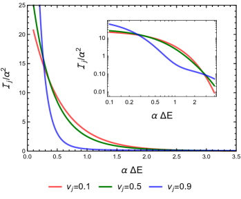
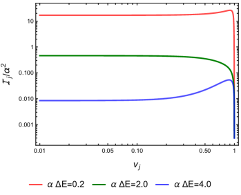
Figure 1: In $(1+1)$ dimensions the integral $\mathcal{I}_{j}$ denoting individual detector transition probability is plotted as functions of $\alpha\,\Delta E$ and $v_{j}$ in the upper and the lower figures respectively. For both the cases we considered the distribution function $f(\omega_{k})=C\,\omega_{k}\,e^{-\alpha\omega_{k}}$. From the upper plot one can observe that in the low $(\alpha\,\Delta E\lesssim 0.26)$ and high $(\alpha\,\Delta E\gtrsim 2.9)$ value regions of $\alpha\,\Delta E$ the transition probability increases with increasing detector velocity upto certain large velocities. While in the intermediate region it decreases with increasing velocity. We mention that the upper inner and the lower plots are presented in Log-Log fashion.

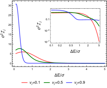
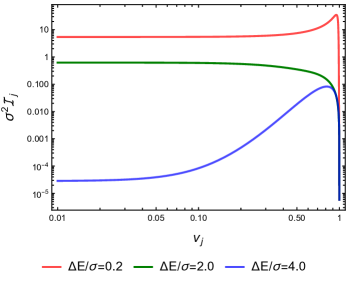
Figure 2: In $(1+1)$ dimensions the integral $\mathcal{I}_{j}$ denoting individual detector transition probability is plotted as functions of $\Delta E/\sigma$ and $v_{j}$ in the upper and the lower figures respectively. For both the cases we considered the distribution function $f(\omega_{k})=C\,\omega_{k}~{}e^{-(\omega_{k}-\omega_{0})^{2}/2\sigma^{2}}$, with $\omega_{0}/\sigma=0.5$. From the upper plot one can observe that in the low $(\Delta E/\sigma\lesssim 0.38)$ and high $(\Delta E/\sigma\gtrsim 3.3)$ value regions of $\Delta E/\sigma$ the transition probability increases with increasing detector velocity upto certain velocities. While in the intermediate region it decreases with increasing velocity. Here also we have presented the upper inner and the lower plots in Log-Log fashion.

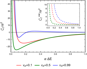
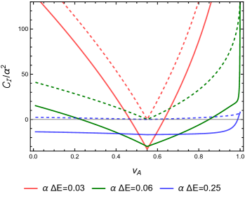
Figure 3: In $(1+1)$ dimensions the quantity $\mathcal{C}_{\mathcal{I}}$ signifying the concurrence (the solid lines) is plotted as functions of $\alpha\,\Delta E$ and $v_{A}$ in the upper and the lower plots respectively. Here the velocity of detector $B$ is fixed at $v_{B}=0.55$. To arrive at these plots we have considered the distribution function $f(\omega_{k})=C\,\omega_{k}\,e^{-\alpha\omega_{k}}$. We also mention that $\mathcal{C}_{\mathcal{I}}^{vac}$, denoted by the dashed lines, indicates the concurrence if the detectors were interacting with the field vacuum. In the lower plot we have chosen the fixed parameter values for $\alpha\,\Delta E$ conveniently as suggested from the upper plot.

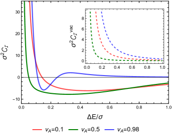
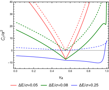
Figure 4: In $(1+1)$ dimensions the quantity $\mathcal{C}_{\mathcal{I}}$ signifying the concurrence (the solid lines) is plotted as functions of $\Delta E/\sigma$ and $v_{A}$ in the upper and the lower plots respectively. We have considered the distribution function $f(\omega_{k})=C\,\omega_{k}~{}e^{-(\omega_{k}-\omega_{0})^{2}/2\sigma^{2}}$ in this case with $\omega_{0}/\sigma=0.5$ and $v_{B}=0.55$. Here also $\mathcal{C}_{\mathcal{I}}^{vac}$ (the dashed lines) indicates the concurrence if the detectors were interacting with the field vacuum.

III.1 Evaluation of $\mathcal{I}_{j}$

The integrals $\mathcal{I}_{j}$ from the quantities $\mathcal{P}_{j}$ signify individual detector transition probabilities. We shall be first evaluating these integrals. Note that in $(1+1)$ dimensions the expression of the scalar field mode function is given by $u_{k}(X_{j})=(1/\sqrt{4\pi\omega_{k}})\,e^{-i\,\omega_{k}\,t_{j}+i\,k\,x_{j}}$ and so the Wightman function is

$$G_{W}(X_{j},X^{\prime}_{j})=\int_{-\infty}^{\infty}\frac{dk}{4\pi\omega_{k}}\,e^{-i\,\omega_{k}\,(t_{j}-t^{\prime}_{j})+i\,k\,(x_{j}-x^{\prime}_{j})}\,.$$ (22)

Utilizing this Wightman function with the coordinate transformation from Eq. (III) one can find out the quantity $\mathcal{I}_{j}^{vac}$ from (19) as

$$\mathcal{I}_{j}^{vac} = \int_{-\infty}^{\infty}\frac{dk}{4\pi\omega_{k}}\,\int_{-\infty}^{\infty}\int_{-\infty}^{\infty}d\tau_{j}\,d\tau^{\prime}_{j}\,e^{-i\Delta{E}(\tau_{j}-\tau^{\prime}_{j})}$$

$$~{}~{}~{}~{}~{}~{}~{}~{}~{}~{}~{}~{}~{}~{}\times\,e^{-i\,(\omega_{k}-k\,v_{j})\,\gamma_{j}(\tau_{j}-\tau^{\prime}_{j})}\,$$

$$= \int_{-\infty}^{\infty}\,\frac{\pi\,dk}{\omega_{k}}\,\left\{\delta[\gamma_{j}\,(\omega_{k}-k\,v_{j})+\Delta E]\right\}^{2}~{}$$

$$= \int_{0}^{\infty}\,\frac{\pi\,d\omega_{k}}{\omega_{k}}\,\Big{[}\left\{\delta[\gamma_{j}\,\omega_{k}(1-\,v_{j})+\Delta E]\right\}^{2}~{}$$ (23)

$$~{}~{}~{}~{}~{}~{}~{}~{}+\,\left\{\delta[\gamma_{j}\,\omega_{k}(1+\,v_{j})+\Delta E]\right\}^{2}\Big{]}\,,$$

where $\omega_{k}=|k|$ has been used. The final expression in Eq. (III.1) vanishes as we have $0\leq v_{j}\leq 1$ and $\Delta E>0$. The reason behind is, in that situation the argument of the Dirac delta distribution is always positive in the considered integration range of $\omega_{k}$. This is expected as an inertial detector does not suffer transition due to vacuum fluctuation of fields.

On the other hand, if one uses the expression of $\Phi_{eff}(X)$ from Eq. (12) for $(1+1)$ dimensions, then the quantity $\mathcal{A}(\Delta E)$, given by Eq. (20a), becomes

$$\mathcal{A}(\Delta E) = \int_{-\infty}^{\infty}\frac{f(\omega_{k})\,dk}{4\pi\omega_{k}}\int_{-\infty}^{\infty}d\tau^{\prime}_{j}\,e^{i[\Delta{E}\,-\,(\omega_{k}-k\,v_{j})\,\gamma_{j}]\tau^{\prime}_{j}}$$

$$= \int_{-\infty}^{\infty}\frac{dk}{2\omega_{k}}\,f(\omega_{k})\,\delta[\gamma_{j}\,(\omega_{k}-k\,v_{j})-\Delta{E}]$$

$$= \frac{1}{2\,\Delta E}\,\left\{f(D_{j}\,\Delta E)+f(\Delta E/D_{j})\right\}~{},$$ (24)

where, $D_{j}=\sqrt{1+v_{j}}/\sqrt{1-v_{j}}$. In a similar manner one can find out the other quantity from (20b) as

$$\mathcal{B}(\Delta E) = \int_{-\infty}^{\infty}\frac{f(\omega_{k})\,dk}{4\pi\omega_{k}}\int_{-\infty}^{\infty}d\tau^{\prime}_{j}\,e^{i[\Delta{E}\,+\,(\omega_{k}-k\,v_{j})\,\gamma_{j}]\tau^{\prime}_{j}}$$

$$= \int_{-\infty}^{\infty}\frac{dk}{2\omega_{k}}\,f(\omega_{k})\,\delta[(\omega_{k}-k\,v_{j})\,\gamma_{j}+\Delta{E}]$$

$$= 0~{},$$ (25)

for $\Delta E>0$. Therefore, in $(1+1)$ dimensions with two detectors in uniform velocities the quantity $\mathcal{I}_{j}$ from Eq. (18) is entirely given by $\mathcal{A}(\Delta E)$, specifically as $\mathcal{I}_{j}(\Delta E)=|\mathcal{A}(\Delta E)|^{2}$. Once the explicit form of distribution function $f(\omega_{k})$ is given, then we will be able to know $\mathcal{I}_{j}(\Delta E)$. One may look into Appendix A.1 for the expressions of a few possible distribution functions $f(\omega_{k})$ in $(1+1)$ dimensions. We choose them to be similar that have been adopted in Lochan and Padmanabhan (2015) to investigate the single detector’s response function in an accelerated frame.

Note that the quantities $\mathcal{I}_{j}$ denote the single detector transition probabilities. Since we have not found any discussions in the literature on transition probabilities of single inertial detectors in flat spacetime interacting with the non-vacuum field states, here we end this subsection with an analysis on the features of this quantity. In particular, in Fig. 1 and 2 we have plotted these quantities for the specific distribution functions $f(\omega_{k})=C\,\omega_{k}\,e^{-\alpha\omega_{k}}$ and $f(\omega_{k})=C\,\omega_{k}~{}e^{-(\omega_{k}-\omega_{0})^{2}/2\sigma^{2}}$ respectively. Here $C$ is the normalization constant and its explicit form, which is imperative for obtaining the numerical value of $\mathcal{I}_{j}$, is determined in Appendix A.1.

From these figures, with both the exponentially damping and Gaussian distribution functions, one can observe that in different regions of $\Delta E$ the transition probability varies differently with the velocity $v_{j}$ of the detector. For example, the upper plots of Fig. 1 and 2 signify that for very low and high $\Delta E$ the transition increases with increasing $v_{j}$. While in the intermediate range of $\Delta E$, transition decreases with increasing $v_{j}$. The behavior of the transition probability with respect to the velocity $v_{j}$ in different $\Delta E$ regimes is further elucidated in the lower plots of the concerned figures. From those plots, one further can observe that in the low and high $\Delta E$ regime, when $\Delta E/\kappa=0.2$ and $\Delta E/\kappa=4$ (here $\kappa$ can be $\sigma$ or $1/\alpha$ depending on the considered distribution function), the transition rate initially increases with increasing velocity $v_{j}$ up to certain values of $v_{j}$ and then decreases. While this characteristic is different in the intermediate transition energy regimes, e.g., when $\Delta E/\kappa=2$. In the later case transition probability decreases with the increase of $v_{j}$.

Let us now elucidate on the reasoning behind the specific features of the lower plots in Figs. 1 and 2, which is due to the appearance of two terms in Eq. (III.1). One is providing red shift in $\Delta E$ while the other one induces blue shift. In order to understand influence of these two effects in the transition amplitude, it is convenient to pay attention on a particular distribution of $f(\omega_{k})$. Here we consider the exponentially damping one, where $\mathcal{A}(\Delta E)$ is given by

$$\mathcal{A}(\Delta E) = \frac{C}{2}\bigg{[}\sqrt{\frac{1+v_{j}}{1-v_{j}}}e^{-\alpha\Delta E\sqrt{\frac{1+v_{j}}{1-v_{j}}}}$$ (26)

$$+ \sqrt{\frac{1-v_{j}}{1+v_{j}}}e^{-\alpha\Delta E\sqrt{\frac{1-v_{j}}{1+v_{j}}}}\,\bigg{]}~{}.$$

Since we have $v_{j}<1$, the above can be expanded in Taylor series. Keeping terms up to leading order in $v_{j}$ (which is here $v_{j}^{2}$) one finds

$$\mathcal{A}(\Delta E)\simeq Ce^{-\alpha\Delta E}\Big{[}1+\left(\alpha^{2}\Delta E^{2}-3\alpha\Delta E+1\right)v_{j}^{2}\Big{]}\,.$$ (27)

Therefore when $\left(\alpha^{2}\Delta E^{2}-3\alpha\Delta E+1\right)>0$, the magnitude of the transition amplitude will increase with the increase of $v_{j}$. But if $\left(\alpha^{2}\Delta E^{2}-3\alpha\Delta E+1\right)<0$, then second term in the above expression provides diminishing effect in amplitude. As a result the transition amplitude decreases with the increase in $v_{j}$. This discussion provides explanation for the nature of curves for $\alpha\Delta E=0.2,2.0$ and $4.0$. But when $v_{j}$ is large, i.e., $v_{j}\to 1$, this approximation is not valid. In that case it is noted that the first term in (26) decays exponentially with the increase of $v_{j}$. Because of the pre-factor in the second exponential, the whole term also decreases. Hence effectively the amplitude decreases with the increase of $v_{j}$. Furthermore, one can check by taking the limit $v_{j}\to 1$ that the transition amplitude $\mathcal{A}(\Delta E)$ vanishes. Similar things are also happening for the Gaussian distribution in the lower plot of Fig. 2.

III.2 Evaluation of $\mathcal{I}_{\varepsilon}$, and the concurrence $\mathcal{C}_{\mathcal{I}}$

Let us now proceed to evaluate the integral $\mathcal{I}_{\varepsilon}$. We first consider the expression of $\mathcal{I}_{\varepsilon}$ from Eq. (14) and evaluate $\mathcal{I}_{\varepsilon}^{vac}$, which again is expressed as (16). In Eq. (16) the term containing only the Wightman function can be expressed as

$$\mathcal{I}_{\varepsilon_{W}}^{vac} = -\frac{1}{\gamma_{A}\gamma_{B}}\int_{-\infty}^{\infty}\frac{dk}{4\pi\omega_{k}}\,\int_{-\infty}^{\infty}dt_{B}\int_{-\infty}^{\infty}dt_{A}~{}$$

$$\times~{}e^{-i(\omega_{k}-k\,v_{B})\,t_{B}+i(\omega_{k}-k\,v_{A})\,t_{A}}$$

$$~{}~{}~{}~{}~{}~{}~{}~{}~{}~{}~{}\times\,e^{i\Delta E(t_{B}/\gamma_{B}+t_{A}/\gamma_{A})}\,$$

$$= -\frac{\pi}{\gamma_{A}\gamma_{B}}\int_{-\infty}^{\infty}\frac{dk}{\omega_{k}}\,\delta[(\omega_{k}-k\,v_{A})+\Delta{E}/\gamma_{A}]$$

$$\times~{}\,\delta[(\omega_{k}-k\,v_{B})-\Delta{E}/\gamma_{B}]\,,$$ (28)

which will vanish due to the first Dirac-delta distribution for $\Delta{E}>0$. We also mention that here we have used the relation $t_{j}=\gamma_{j}\,\tau_{j}$ from Eq. (III). On the other hand, from Eq. (16) the term containing the retarded Green’s function can be expressed as

$$\mathcal{I}_{\varepsilon_{R}}^{vac}$$

$$=\frac{i}{\gamma_{A}\gamma_{B}}\int_{-\infty}^{\infty}\frac{dk}{2\omega_{k}}\,\Bigg{[}\frac{\delta[k(v_{A}-v_{B})-\Delta{E}(1/\gamma_{A}+1/\gamma_{B})]}{\omega_{k}-k\,v_{B}-\Delta{E}/\gamma_{B}}$$

$$~{}~{}~{}+~{}\frac{\delta[k(v_{A}-v_{B})+\Delta{E}(1/\gamma_{A}+1/\gamma_{B})]}{\omega_{k}-k\,v_{B}+\Delta{E}/\gamma_{B}}\Bigg{]}\,.$$ (29)

See Appendix B for an explicit derivation of this expression. Here we have also used the fact that the Minkowski time $t_{j}$ are the temporal coordinates $T_{j}$ for field mode expansion in (17). For $v_{A}>v_{B}$ this expression leads to

$$\mathcal{I}_{\varepsilon_{R}}^{vac} = \frac{i\gamma_{A}\gamma_{B}(v_{A}-v_{B})D_{A}D_{B}}{\Delta E^{2}(D_{A}+D_{B})^{2}}\,~{}.$$ (30)

On the other hand, for $v_{B}>v_{A}$ the integral from Eq. (III.2) becomes

$$\mathcal{I}_{\varepsilon_{R}}^{vac} = \frac{i\gamma_{A}\gamma_{B}(v_{B}-v_{A})D_{A}D_{B}}{\Delta E^{2}(D_{A}+D_{B})^{2}}~{},$$ (31)

which is basically the same compared to the expression from $v_{A}>v_{B}$ case with a change in sign. From the previous sub-section we have seen that the integral of the form $\int_{-\infty}^{\infty}d\tau\,e^{i\Delta{E}\,\tau}\,\Phi_{eff}^{\star}(\tau)$ vanishes for detectors in uniform velocity in $(1+1)$ dimensions (see Eq. (26)). Then, one can perceive that the quantity $\mathcal{I}_{\varepsilon}^{nv}$ from Eq. (15) will also vanish in this scenario. Therefore, in this case we have $\mathcal{I}_{\varepsilon}$ entirely given by $\mathcal{I}_{\varepsilon_{R}}^{vac}$, i.e., $\mathcal{I}_{\varepsilon}=\mathcal{I}_{\varepsilon_{R}}^{vac}$. Moreover, since there is only a sign change between the expressions from Eq. (30) and (31), in both the cases $v_{A}>v_{B}$ and $v_{A}<v_{B}$ the quantity $|\mathcal{I}_{\varepsilon}|$ appearing in (8) yields the same feature. Also observe from Eq. (30) and (31) that when $v_{A}=v_{B}$ the integral $\mathcal{I}_{\varepsilon}$ vanishes and so vanishes the concurrence. Thus in a situation when the two UD detectors are co-moving in $(1+1)$ dimensions there will be no entanglement harvesting. On the other hand, when the velocity of detector $A$ approaches the velocity of light, i.e., when $v_{A}\to 1$, the quantity $|\mathcal{I}_{\varepsilon_{R}}^{vac}|=1/(2\Delta E^{2})$. Therefore, in this limit there is an upper bound in the value of the concurrence depending on the value of $v_{B}$ and $\Delta E$. This expressions also suggests that in this limit the amount of harvested concurrence (see Eq. (8)) should be increasing with decreasing $\Delta E$.

In Fig. 3 and 4 we have plotted the concurrence denoting quantity $\mathcal{C}_{\mathcal{I}}$ as described in Eq. (8) considering the exponentially damping and Gaussian distribution functions respectively. For a discussion on these distributions in $(1+1)$ dimensions see Appendix A.1. We also mention that if the detectors were to interact with the field vacuum rather than the singly excited field state, the quantities $\mathcal{I}_{j}$ denoting single detectors’ transition probabilities would have been zero. In that scenario the concurrence is entirely given by $\mathcal{C}_{\mathcal{I}}^{vac}=|\mathcal{I}_{\varepsilon}|=|\mathcal{I}_{\varepsilon_{R}}^{vac}|$, a depiction of which is also included in these plots. From these figures, one notices that when $v_{A}=v_{B}$, the entanglement harvesting, like vacuum field state, ceases to exist for non-vacuum field state as well. Fig. 3 and 4 also confirms the possibility of entanglement harvesting between inertial UD detectors even from the single particle field states in $(1+1)$ dimensions. However, comparing the plots for $\mathcal{C}_{\mathcal{I}}$ and $\mathcal{C}_{\mathcal{I}}^{vac}$ from these figures, one can clearly see that entanglement harvesting is reduced in the non-vacuum case. In the non-vacuum situation the reduction happens not only in magnitude of concurrence, also the range of velocity decreases. A common feature observed with both the distributions (the exponential damping and Gaussian distributions) is that the regime of low detector transition energy corresponds to quantitatively higher entanglement extraction. One should also note that for large fixed transitions energies there is no entanglement harvesting from the low velocity regimes. However, the amount of the harvested entanglement in the high velocity regime keeps decreasing with increasing $\Delta E$. This is because in the very large $v_{A}$ limit the entangling term varies as $\sim 1/(\Delta E)^{2}$ and hence $\mathcal{I}_{\varepsilon}$ increase more than $\mathcal{I}_{j}$ with the decrease of $\Delta E$.

IV Entanglement harvesting: motion in $(1+3)$ dimensions

Now we are going to investigate the same in $(1+3)$ dimensions. Since there are three spacial directions, the observers can move in more than one possible directions. We mainly concentrate on following motions of the two detectors – both are moving along the same direction and one is moving in the perpendicular direction of the other’s motion.

IV.1 Parallel motion

In this part we we are going to consider Unruh-DeWitt detectors in parallel uniform velocities in $(1+3)$ dimensions. For simplicity we shall consider the detectors to be in motion along the $z$ direction. In particular, the observer with detector $A$ is assumed to have an inertial motion such that its coordinates are related to its proper time as

$$t_{A}=\gamma_{A}\tau_{A};~{}~{}x_{A}=0;~{}~{}y_{A}=0;~{}~{}z_{A}=\gamma_{A}v_{A}\tau_{A}.$$ (32)

On the other hand, the trajectory of detector $B$ is

$$t_{B}=\gamma_{B}\tau_{B};~{}~{}x_{B}=x_{0};~{}~{}y_{B}=y_{0};~{}~{}z_{B}=\gamma_{B}v_{B}\tau_{B},$$ (33)

such that $r_{0}=\sqrt{x_{0}^{2}+y_{0}^{2}}$ is the perpendicular distance between the two detectors $A$ and $B$. In $(1+3)$ dimensions the effective field $\Phi_{\text{eff }}$ with respect to the Minkowski modes is given as

$$\Phi_{\mathrm{eff}}(x)=\int\frac{d^{3}k}{(2\pi)^{3}}\frac{f(\omega_{k})}{2\omega_{k}}e^{ik\cdot x}~{},$$ (34)

where, $k\cdot x\equiv k_{a}x^{a}=-\omega_{k}t+\vec{k}\cdot\vec{x}~{}$. We shall see that unlike the previous $(1+1)$ dimensional scenario, here the expressions of $\mathcal{I}_{A}$ and $\mathcal{I}_{B}$ are not the same due to a finite non-zero initial separation between the two detectors.

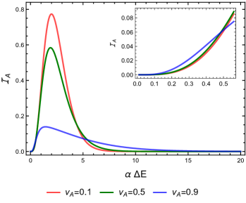
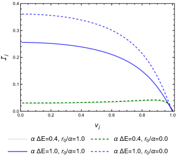
Figure 5: In the upper figure the integral $\mathcal{I}_{A}$ (which signifies individual detector transition probability) is plotted as a function of $\alpha\,\Delta E$ for fixed values of $v_{A}$ in $(1+3)$ dimensions. On the other hand, in the lower figure $\mathcal{I}_{j}$ is plotted with respect to $v_{j}$ for different fixed values of $\alpha\,\Delta E$ and $r_{0}/\alpha$. In both of these figures we have considered the distribution function $f(\omega_{k})=C~{}\omega_{k}~{}e^{-\alpha\omega_{k}}$. It is to be noted that in the lower plot $r_{0}/\alpha=1$ corresponds to detector $B$ and $r_{0}/\alpha=0$ corresponds to detector $A$. From the upper figure one can observe that in different regions of $\alpha\,\Delta E$ the transition probability may increase or decrease with increasing detector velocity. This observation is similar to the ones from $(1+1)$ dimensions, see Fig. 1.

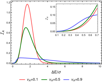
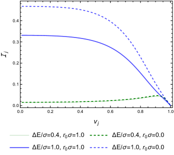
Figure 6: In the upper figure $\mathcal{I}_{A}$ is plotted as a function of $\Delta E/\sigma$ for fixed values of $v_{A}$ in $(1+3)$ dimensions. On the other hand, in the lower figure $\mathcal{I}_{j}$ is plotted with respect to $v_{j}$ for different fixed values of $\Delta E/\sigma$ and $r_{0}\sigma$. In both of these figures we have considered the distribution function $f(\omega_{k})=C~{}\omega_{k}~{}e^{-(\omega_{k}-\omega_{0})^{2}/2\sigma^{2}}$ with $\omega_{0}/\sigma=0.5$. Here also in the lower plot $r_{0}\sigma=1$ corresponds to detector $B$ and $r_{0}\sigma=0$ corresponds to detector $A$.

IV.1.1 Evaluation of $\mathcal{I}_{j}$

Let us consider evaluating the integral $\mathcal{I}_{B}$ first, and one may expect that the expression of the integral $\mathcal{I}_{A}$ will arrive as a special case when $r_{0}=0$. For trajectory given in (33) the integral $\mathcal{I}_{B}$ can be evaluated considering the wave-vector in the spherical polar coordinates such that

$$k\cdot x = -\omega_{k}t+\vec{k}.\vec{x}$$ (35)

$$= \omega_{k}(-\gamma_{B}\tau_{B}+x_{0}\sin\theta\cos\phi$$

$$~{}~{}~{}~{}~{}~{}+y_{0}\sin\theta\sin\phi+v_{B}\gamma_{B}\tau_{B}\cos\theta)~{},$$

where we have used

$$\vec{k} = \omega_{k}\left(\sin\theta\cos\phi\,\hat{x}+\sin\theta\sin\phi\,\hat{y}+\cos\theta\,\hat{z}\right)~{},$$

$$\vec{x} = x\,\hat{x}+y\,\hat{y}+z\,\hat{z}~{},$$ (36)

with $\omega_{k}=|\vec{k}|$. Then in this case one can obtain the quantity from Eq. (20a) as

$$\mathcal{A}_{B}(\Delta E) = \int_{-1}^{1}\frac{du}{4\pi}\frac{\Delta E\,f\left(\frac{\Delta E}{\gamma_{B}(1-v_{B}u)}\right)}{\left[\gamma_{B}(1-v_{B}u)\right]^{2}}J_{0}\left(\tfrac{r_{0}\Delta E\sqrt{1-u^{2}}}{\gamma(1-v_{B}u)}\right)~{},$$

where $J_{n}(x)$ denotes the Bessel function of the first kind, and $r_{0}=\sqrt{x_{0}^{2}+y_{0}^{2}}$. A detailed derivation of this expression is presented in Appendix C. From this expression one can easily find out the value of $\mathcal{A}(\Delta E)$ for detector $A$ by making $r_{0}=0$ as is also evident from the trajectories (32) and (33). When $r_{0}=0$ and $v_{B}\to v_{A}$ one may consider a change of variables $z=\Delta E/\gamma_{A}(1-v_{A}u)$ in the previous equation such that it reduces to

$$\mathcal{A}_{A}(\Delta E)=\frac{1}{4\pi v_{A}\gamma_{A}}\int_{\Delta E/D_{A}}^{D_{A}\Delta E}\,dz\,f(z)~{}.$$ (38)

where we have used the fact that $J_{0}(0)=1$. This expression matches exactly with the one obtained explicitly for the detector $A$ with trajectory (32), and is provided in Appendix C. The relevant expression is derived in Eq. (63) of the Appendix. One should notice that in Eq. (38) and (IV.1.1) we have included subscript $A$ and $B$ to signify the specific detectors. One may find out the respective $\mathcal{I}_{j}$ from $\mathcal{I}_{j}=|\mathcal{A}_{j}(\Delta E)|^{2}$ as here also $\mathcal{I}_{j}^{vac}=0$ and $\mathcal{B}(\Delta E)=0$ (see Appendix C for details).

In $(1+3)$ dimensions one may use the expressions of a few possible distribution functions as given in Appendix A.2 to obtain $\mathcal{I}_{j}$. In particular, in Appendix A.2 the explicit forms of the normalization constants $(C)$ in the exponential damping and the Gaussian distribution functions are obtained, which are essential for procuring a numerical value for the above mentioned integral. Here also, these quantities $\mathcal{I}_{j}$ correspond to individual detector transition probabilities with a non-vacuum singly excited field state in the background. We have plotted this transition probability in Fig. 5 and 6 for the exponential decaying and Gaussian distribution functions, respectively. To be specific, we have plotted the quantity $\mathcal{I}_{B}$ with respect to the velocity $v_{B}$ (when $r_{0}\neq 0$), where the special case of $r_{0}=0$ produces the transition probability $\mathcal{I}_{A}$ with $v_{B}$ now becoming $v_{A}$. The curves in these plots have somewhat similar features to the ones from $(1+1)$ dimensions. Specifically, for low and high transition energy $\Delta E$, the transition probability increases with increasing velocity, and in the intermediate $\Delta E$ regimes this nature is reversed. Also visible from these plots is that the transition probability decreases with increasing $r_{0}$.

IV.1.2 Evaluation of $\mathcal{I}_{\varepsilon}$, and $\mathcal{C}_{\mathcal{I}}$

Let us now evaluate the integral $\mathcal{I}_{\varepsilon}$ for these two detectors which are in parallel inertial motion. In this scenario the quantities $\mathcal{I}_{\varepsilon}^{nv}$ and $\mathcal{I}_{\varepsilon_{W}}^{vac}$ vanish. The detailed calculation is provided in Appendix C. The only non-vanishing contribution is given by the integral $\mathcal{I}_{\varepsilon_{R}}^{vac}$. Using the representation from Eq. (17) and with the help of Eqs. (32) and (33) one can express this integral as

$$\mathcal{I}_{\varepsilon_{R}}^{vac} = -\int_{-\infty}^{\infty}\int_{-\infty}^{\infty}\frac{dp~{}dq}{2v_{A}v_{B}^{\prime}\gamma_{A}\gamma_{B}}e^{i\Delta{E}(a_{1}p+a_{2}q)}\theta(a_{3}p-q)$$

$$\times\int_{-1}^{1}du\int_{0}^{\infty}\frac{\omega_{k}d\omega_{k}}{2(2\pi)^{2}}\Big{[}e^{-i\omega_{k}a_{4}(a_{3}p-q)+i\omega_{k}\sqrt{p^{2}+r_{0}^{2}}u}$$

$$~{}~{}~{}~{}~{}~{}~{}~{}~{}~{}~{}~{}~{}~{}~{}~{}~{}~{}~{}~{}~{}~{}~{}~{}~{}-e^{i\omega_{k}a_{4}(a_{3}p-q)-i\omega_{k}\sqrt{p^{2}+r_{0}^{2}}u}\Big{]},$$

where we have considered the change of variables $p=v_{A}\gamma_{A}\tau_{A}-v_{B}\gamma_{B}\tau_{B}$ and $q=v_{A}\gamma_{A}\tau_{A}+v_{B}\gamma_{B}\tau_{B}$. The Jacobian of this transform is given by $|J|=1/(2v_{A}v_{B}\gamma_{A}\gamma_{B})$. Whereas, the other variable is $u=\cos{\theta}$, and we have considered the redefined parameters $a_{1}=1/(2v_{A}\gamma_{A})-1/(2v_{B}\gamma_{B})$, $a_{2}=1/(2v_{A}\gamma_{A})+1/(2v_{B}\gamma_{B})$, $a_{3}=(v_{A}+v_{B})/(v_{A}-v_{B})$, and $a_{4}=(v_{A}-v_{B})/2v_{A}v_{B}$. One may notice that due to the Heaviside step function the upper limit of the $q$ integration transforms to $a_{3}p$. Then one may evaluate this entire quantity $\mathcal{I}_{\varepsilon_{R}}^{vac}$ in a step by manner with first carrying out the integration over $q$. Subsequently the integrals over $u$ and $\omega_{k}$ can be performed in a likewise manner. After carrying out all these steps the integral looks like

$$\mathcal{I}_{\varepsilon_{R}}^{vac}=\int_{-\infty}^{\infty}dp\,\frac{i\,e^{i\Delta{E}p(a_{1}+a_{2}a_{3})}\cos\left(\tfrac{a_{2}\Delta{E}\sqrt{p^{2}+r_{0}^{2}}}{a_{4}}\right)}{8\pi v_{A}v_{B}\gamma_{A}\gamma_{B}a_{4}\sqrt{p^{2}+r_{0}^{2}}}\,.$$ (40)

To perceive a detailed procedure to arrive at this expression one may look into Appendix C.3.2. This integral can be carried out to give a further simplified expression with the help of the integral representations of the modified Bessel function of the second kind $K_{n}(z)$ (see Eq. (3.876) of Gradshteyn and Ryzhik (2014)), which are

$$\int_{0}^{\infty}\frac{\cos\left(\varrho\sqrt{\xi^{2}+a^{2}}\right)}{\sqrt{\xi^{2}+a^{2}}}\cos(\beta\xi)\mathrm{~{}d}\xi = K_{0}\left(a\sqrt{\beta^{2}-\varrho^{2}}\right)~{};$$

$$\int_{0}^{\infty}\frac{\sin\left(\varrho\sqrt{\xi^{2}+a^{2}}\right)}{\sqrt{\xi^{2}+a^{2}}}\cos(\beta\xi)\mathrm{~{}d}\xi = 0\,,~{}{[\beta>\varrho>0]}\,.$$ (41)

Now one can observe that the exponential in the integral (40) can be written in terms of $\sin$ and $\cos$ functions so that the previous forms of Eq. (IV.1.2) can be perceived. In our case, a comparison with Eq. (IV.1.2) reveals $\beta=\Delta{E}(a_{1}+a_{2}a_{3})$ and $\varrho=a_{2}\Delta{E}/a_{4}$. Then from the consideration of a positive transition frequency $\Delta E$ (which is true in our case) and the explicit expressions of $a_{1}$, $a_{2}$, $a_{3}$, and $a_{4}$ one can confirm the satisfaction of the condition $\beta>\varrho>0$ even with the integral (40). In particular, the integral of Eq. (40) now becomes

$$\mathcal{I}_{\varepsilon_{R}}^{vac} = i\int_{0}^{\infty}dp\,\frac{\cos\left(\frac{a_{2}\Delta{E}}{a_{4}}\sqrt{p^{2}+r_{0}^{2}}\right)}{2\pi(v_{A}-v_{B})\gamma_{A}\gamma_{B}\sqrt{p^{2}+r_{0}^{2}}}$$

$$~{}~{}~{}~{}~{}~{}~{}~{}~{}~{}~{}~{}~{}~{}~{}\times~{}\cos\left\{\Delta{E}p(a_{1}+a_{2}a_{3})\right\}$$ (42)

$$= \frac{i~{}K_{0}\left(r_{0}\Delta{E}\sqrt{\left(a_{1}+a_{2}a_{3}\right)^{2}-\left(a_{2}/a_{4}\right)^{2}}\right)}{2\pi(v_{A}-v_{B})\gamma_{A}\gamma_{B}}$$

$$= \frac{-i}{2\pi\gamma_{A}\gamma_{B}(v_{A}-v_{B})}$$

$$\times K_{0}\left(\tfrac{r_{0}\Delta{E}}{\gamma_{B}}\sqrt{\left(\tfrac{\frac{1}{\gamma_{A}}+\gamma_{B}(1-v_{A}v_{B})}{v_{A}-v_{B}}\right)^{2}-\gamma_{B}^{2}}\right),~{}~{}~{}~{}$$

where we have used (IV.1.2) along with the relation $2v_{A}v_{B}a_{4}=(v_{A}-v_{B})$.

As a side remark and for comparison with the earlier result (given in Koga et al. (2018)) we mention that in the limit $v_{B}\to 0$ we have $(a_{1}+a_{2}a_{3})^{2}-(a_{2}/a_{4})^{2}=2(1+\gamma_{A})/v_{A}^{2}\gamma_{A}^{2}$, and thus the expression of $\mathcal{I}_{\varepsilon}$ (which is entirely determined by $\mathcal{I}_{\varepsilon_{R}}^{vac}$) is given by

$$\left|\mathcal{I}_{\varepsilon}\right|=\frac{1}{2\pi v_{A}\gamma_{A}}K_{0}\left(\frac{r_{0}\Delta{E}}{v_{A}\gamma_{A}}\sqrt{2(1+\gamma_{A})}\right)~{}.$$ (43)

This result matches correctly with the one from Koga et al. (2018) (see Eq. (74) of Koga et al. (2018) with $\theta=\pi/2$, where $\theta$ is the angle between $\vec{v}$ and $\vec{x}_{0}$), where one of the detectors was taken to be static.

We should emphasize here that in our present case the quantities $\mathcal{I}_{\varepsilon_{W}}^{vac}$ and $\mathcal{I}_{\varepsilon}^{nv}$ vanish (see Appendix C for detailed estimations of these integrals).

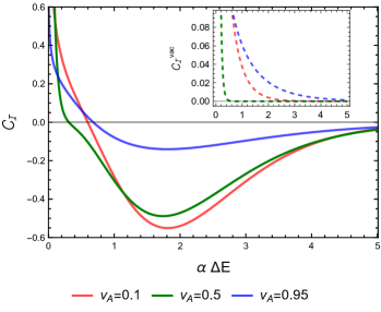
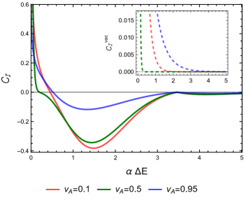
Figure 7: In $(1+3)$ dimensions the integral $\mathcal{C}_{\mathcal{I}}$ signifying the concurrence is plotted as a function of $\alpha\,\Delta E$ for different fixed values of $v_{A}$ with two detectors in parallel inertial motion. In this plot we have considered the distribution function $f(\omega_{k})=C\,\omega_{k}\,e^{-\alpha\omega_{k}}$ for the singly excited background field state. Here the velocity of detector $B$ is fixed at $v_{B}=0.55$ and the other parameter is $r_{0}/\alpha=0.5$ and $r_{0}/\alpha=1$ respectively in the upper and lower plots. These curves assert that entanglement harvesting from single particle field state is possible in the low $\alpha\,\Delta E$ regimes. The inner plots correspond to $\mathcal{C}_{\mathcal{I}}^{vac}$, the concurrence, if the detectors were interacting with the field vacuum.

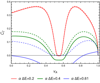
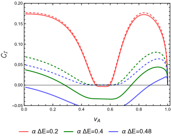
Figure 8: In $(1+3)$ dimensions the integral $\mathcal{C}_{\mathcal{I}}$ signifying the concurrence is plotted as a function of $v_{A}$ for two detectors in parallel inertial motion. The upper and the lower plots respectively correspond to $r_{0}/\alpha=0.5$ and $r_{0}/\alpha=1$. In both of these plots we have considered the distribution function $f(\omega_{k})=C\,\omega_{k}\,e^{-\alpha\omega_{k}}$ for the singly excited background field state. Here the velocity of detector $B$ is fixed at $v_{B}=0.55$. From these plots it is evident that with decreasing $\alpha\,\Delta E$ and $r_{0}/\alpha$ the concurrence increases. The solid lines denote the contributions from $\mathcal{C}_{\mathcal{I}}$, while the dashed lines denote $\mathcal{C}_{\mathcal{I}}^{vac}$.

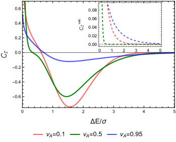
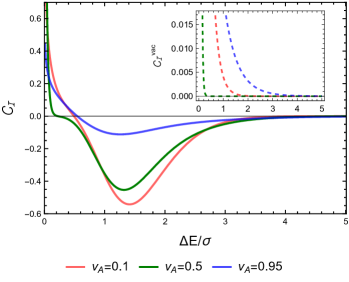
Figure 9: In $(1+3)$ dimensions the integral $\mathcal{C}_{\mathcal{I}}$ signifying the concurrence is plotted as a function of $\Delta E/\sigma$ for different fixed values of $v_{A}$ with two detectors in parallel inertial motion. In this plot we have considered the distribution function $f(\omega_{k})=C\,\omega_{k}~{}e^{-(\omega_{k}-\omega_{0})^{2}/2\sigma^{2}}$ for the singly excited background field state. Here the velocity of detector $B$ is fixed at $v_{B}=0.55$ and the other fixed parameters are $r_{0}\sigma=0.5$ and $r_{0}\sigma=1$ (respectively for the upper and lower figures), $\omega_{0}/\sigma=0.5$. Here also one can observed that entanglement harvesting from single particle field state is possible in the low $\Delta E/\sigma$ regimes. The inner plots correspond to $\mathcal{C}_{\mathcal{I}}^{vac}$, the concurrence, if the detectors were interacting with the field vacuum.

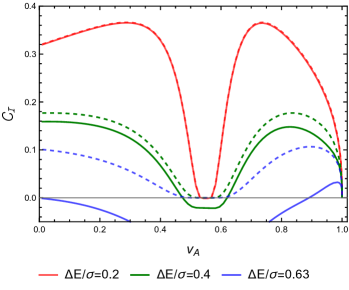
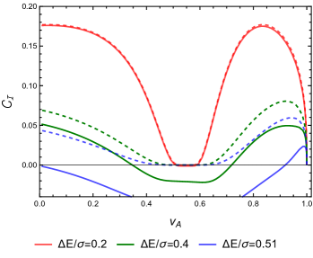
Figure 10: In $(1+3)$ dimensions the integral $\mathcal{C}_{\mathcal{I}}$ signifying the concurrence is plotted as a function of $v_{A}$ for two detectors in parallel inertial motion. The upper and the lower plots respectively correspond to $r_{0}\,\sigma=0.5$ and $r_{0}\,\sigma=1$. In both of these plots we have considered the distribution function $f(\omega_{k})=C\,\omega_{k}~{}e^{-(\omega_{k}-\omega_{0})^{2}/2\sigma^{2}}$ for the singly excited background field state. Here the velocity of detector $B$ is fixed at $v_{B}=0.55$, and the other parameter $\omega_{0}/\sigma=0.5$. From these plots it is evident that with decreasing $\Delta E/\sigma$ and $r_{0}\,\sigma$ the concurrence increases. The solid lines denote the contributions from $\mathcal{C}_{\mathcal{I}}$, while the dashed lines denote $\mathcal{C}_{\mathcal{I}}^{vac}$.

Here one may notice that in the limit of $(v_{A}-v_{B})\to 0$ Eq. (IV.1.2) leads to vanishing result. Therefore, for two parallel co-moving detectors the quantity dictating entanglement harvesting vanishes and one can assert that in this situation there will be no entanglement harvesting. A similar conclusion can also be made starting from Eq. (43), where one of the two observers is static, that the quantity $\left|\mathcal{I}_{\varepsilon}\right|$ vanishes in the limit $v_{A}\to 0$.

In Fig. 7, 8, 9, and 10 we have plotted the concurrence denoting quantity $\mathcal{C}_{\mathcal{I}}$ for different distribution functions of the single particle field state. One can notice from these figures (specifically Fig. 7 and 9) that with decreasing $\Delta E$ the concurrence quantitatively increases, signifying an increase in the measure of the harvested entanglement. While from Fig. 8 and 10 it is evident that when $v_{A}\to v_{B}$ the entanglement harvesting vanishes. Moreover, when the detector transition energy $\Delta E$ becomes larger we observe a wide region of no harvesting around $v_{A}=v_{B}$ and this increases with the increase of $\Delta E$. When the $\Delta E$ value is very large the entanglement harvesting is happening only in high velocity regimes. From Eq. (43) one can observe that in the limit $v_{A}\to 1$ the quantity $\left|\mathcal{I}_{\varepsilon}\right|$ vanishes, and this feature is apparent from these figures too. One should also note that if the detectors were interacting with the field vacuum rather than the non-vacuum state, the quantity $\mathcal{I}_{j}$ would have been zero and the concurrence would have been completely given by $\mathcal{C}_{\mathcal{I}}^{vac}=\left|\mathcal{I}_{\varepsilon}\right|$. We have included the plots of these $\mathcal{C}_{\mathcal{I}}^{vac}$ in the above mentioned figures. Here also, like the $(1+1)$ dimensional case, the entanglement harvesting is suppressed due to non-vacuum fluctuations as compared to vacuum effect. Here both the magnitude of concurrence and valid region of the value of $v_{A}$ for entanglement harvesting decreases. From these figures we also observe that entanglement harvesting is decreasing with increasing distance $r_{0}/\alpha$ between the parallel paths, and with increasing detector transition energy $\Delta E$.

IV.2 Perpendicular motion

In this part we consider two Unruh-DeWitt detectors in motion perpendicular to each other. We consider detector $A$ with an uniform velocity along the $x$-axis and detector $B$ with an uniform velocity along the $z$ direction starting from a constant displacement in the $y$ direction. The trajectory of detector $A$ is

$$t_{A}=\gamma_{A}\tau_{A};~{}~{}x_{A}=\gamma_{A}v_{A}\tau_{A};~{}~{};~{}~{}y_{A}=0;~{}~{}z_{A}=0~{}.$$ (44)

On the other hand, the trajectory of detector $B$ is given by

$$t_{B}=\gamma_{B}\tau_{B};~{}~{}x_{B}=0;~{}~{}y_{B}=r_{0};~{}~{}z=\gamma_{B}v_{B}\tau_{B}~{}.$$ (45)

These trajectories signify that the motion of the detectors are confined to the $x-z$ plane, while there is a perpendicular initial separation between them in the $y$ direction.

IV.2.1 Evaluation of $\mathcal{I}_{j}$

One may observe that the trajectory of the detector $A$ in this case and the previous case of the parallel motion are physically the same. Therefore, the expressions of the integral $\mathcal{I}_{A}$ will also be the same. In fact this indeed comes to be true and one can look into Appendix D.1 for a derivation of the expression of $\mathcal{I}_{A}$ with the trajectory (44). Here we recall the expression of $\mathcal{A}_{A}(\Delta E)$ from Eq. (38), which is relevant to estimate $\mathcal{I}_{A}$, as

$$\mathcal{A}_{A}(\Delta E)=\frac{1}{4\pi v_{A}\gamma_{A}}\int_{\Delta E/D_{A}}^{D_{A}\Delta E}\,dz\,f(z)~{}.$$ (46)

On the other hand, in a similar manner one can also find out the quantity $\mathcal{A}_{B}(\Delta E)$ relevant for estimating $\mathcal{I}_{B}$ with the trajectory (45) as

$$\mathcal{A}_{B}(\Delta E) = \int_{-1}^{1}\frac{du}{4\pi}\frac{\Delta E~{}f\left(\frac{\Delta E}{\gamma_{B}(1-v_{B}u)}\right)}{[\gamma_{B}(1-v_{B}u)]^{2}}J_{0}\left(\tfrac{r_{0}\Delta E\sqrt{1-u^{2}}}{\gamma_{B}(1-v_{B}u)}\right)\,.$$

This expression can be obtained from Eq. (IV.1.1) as the trajectories of detector $B$ from the parallel and perpendicular motion cases are physically equivalent. In this regard, compare the trajectories of detector $B$ from Eq. (33) and (45). Furthermore, one can find that here also $\mathcal{I}_{j}^{vac}=0$ and $\mathcal{B}_{j}(\Delta E)=0$, see Appendix D for details. Then the previous integral signifying individual detector transition probability for the detectors $A$ and $B$ are given by $\mathcal{I}_{j}=|\mathcal{A}_{j}(\Delta E)|^{2}$.

Here with the two detectors in inertial motion perpendicular to each other in $(1+3)$ dimensions, the integrals $\mathcal{I}_{j}$ are the same as the previous parallel case (see Eq. (38) and (IV.1.1) and compare them with the expressions here). Therefore the individual detector’s response function will have the same features as shown in Fig. 5 and 6.

IV.2.2 Evaluation of $\mathcal{I}_{\varepsilon}$, and $\mathcal{C}_{\mathcal{I}}$

Now we shall evaluate the quantity $\mathcal{I}_{\varepsilon}$ for two detectors in perpendicular inertial motion with trajectories given in (44) and (45). In particular, here also one can observe that the $\mathcal{I}_{\varepsilon}^{nv}$ part of this quantity vanishes, so does the $\mathcal{I}_{\varepsilon_{W}}^{vac}$. Then $\mathcal{I}_{\varepsilon}=\mathcal{I}_{\varepsilon}^{nv}+\mathcal{I}_{\varepsilon_{W}}^{vac}+\mathcal{I}_{\varepsilon_{R}}^{vac}$ is completely given by $\mathcal{I}_{\varepsilon_{R}}^{vac}$. In Eq. (17) we have seen that this integral is dependent on the retarded Green’s function $G_{R}\left(X_{A},X_{B}\right)$. This retarded Green function $G_{R}\left(X_{A},X_{B}\right)$ for a massless, minimally coupled, free scalar field in the Minkowski spacetime (see Koga et al. (2018)) is expressed as

$$G_{R}\left(X_{A},X_{B}\right) = -\frac{1}{2\pi}~{}\Theta\left(t_{A}-t_{B}\right)$$

$$~{}~{}\times~{}\delta\left(\left(t_{A}-t_{B}\right)^{2}-\left|\bm{x}_{A}-\bm{x}_{B}\right|^{2}\right)$$ (48)

$$= -\frac{1}{2\pi}\Theta\left(t_{A}-t_{B}\right)\delta(g(t_{A},t_{B}))~{}.$$

For the considered trajectories of detector $A$ and $B$ from Eq. (44) and (45) one can find the solution of $g(t_{A},t_{B})=t_{A}^{2}(1-v_{A}^{2})+t_{B}^{2}(1-v_{B}^{2})-2t_{A}t_{B}-r_{0}^{2}=0$ with respect to $t_{B}$ as

$$t_{B}=\gamma_{B}^{2}(t_{A}\pm u(t_{A}))\equiv t_{\pm}~{},$$ (49)

with,

$$u(t_{A})=\sqrt{t_{A}^{2}(v_{A}^{2}+v_{B}^{2}-v_{A}^{2}v_{B}^{2})+r_{0}^{2}(1-v_{B}^{2})}~{},$$ (50)

where, for $0\leq v_{j}\leq 1$ one can confirm that,

$$\gamma_{B}^{2}(t_{A}+u(t_{A}))>t_{A}$$

$$\gamma_{B}^{2}(t_{A}-u(t_{A}))<t_{A}~{}.$$ (51)

Now it is imperative to use the property of Dirac delta distributions

$$\delta(g(t_{A},t_{B})) = \left[\frac{\delta(t_{B}-t_{+})}{|g^{\prime}(t_{A},t_{B})|_{t_{B}=t_{+}}}+\frac{\delta(t_{B}-t_{-})}{|g^{\prime}(t_{A},t_{B})|_{t_{B}=t_{-}}}\right]$$ (52)

$$= \frac{1}{2u(t_{A})}[\delta(t_{B}-t_{+})+\delta(t_{B}-t_{-})]~{}.$$

Then the integral $\mathcal{I}_{\varepsilon_{R}}^{vac}$ from Eq. (17), with a change of variable from $\tau_{j}$ to $t_{j}$, can be expressed as

$$\mathcal{I}_{\varepsilon_{R}}^{vac} = \frac{-i}{2\pi}\int_{-\infty}^{\infty}{\frac{dt_{A}}{\gamma_{A}}}\int_{-\infty}^{t_{A}}{\frac{dt_{B}}{\gamma_{B}}}\scalebox{0.9}{$e^{i\Delta{E}\big{(}\frac{t_{A}}{\gamma_{A}}+\frac{t_{B}}{\gamma_{B}}\big{)}}\delta(g(t_{A},t_{B}))$}$$

$$= \frac{-i}{4\pi}\int_{-\infty}^{\infty}{\frac{dt_{A}}{\gamma_{A}\gamma_{B}~{}u(t_{A})}}e^{i\Delta{E}\left(\frac{t_{A}}{\gamma_{A}}+\gamma_{B}(t_{A}-u(t_{A})\right)}$$

$$= \frac{-i}{2\pi\gamma_{A}\gamma_{B}}\int_{0}^{\infty}\scalebox{0.95}{$\frac{dt_{A}e^{-i\Delta{E}\gamma_{B}u(t_{A})}}{u(t_{A})}\cos$}\scalebox{0.85}{$\left\{\Delta{E}t_{A}\left(\frac{1}{\gamma_{A}}+\gamma_{B}\right)\right\}$}~{}.$$

Furthermore, one can expand the exponential in this integral in terms of $\sin$ and $\cos$ functions and then by comparing them with the integral representations of the Bessel functions (IV.1.2), can recognize

$$a=r_{0}/\gamma_{B};~{}~{}p=\gamma_{B}\Delta{E};~{}~{}b=\frac{\Delta{E}\left(\frac{1}{\gamma_{A}}+\gamma_{B}\right)}{\sqrt{v_{A}^{2}+v_{B}^{2}(1-v_{A}^{2})}};$$ (54)

and as one has $0\leq v_{j}\leq 1$, this also satisfies the condition among the parameters from (IV.1.2), which is $b>p~{}$. Thus, the integration in Eq. (IV.2.2) can be evaluated. One can provide the simplified form as

$$\mathcal{I}_{\varepsilon_{R}}^{vac} = \frac{-i}{2\pi\gamma_{A}\gamma_{B}\sqrt{v_{A}^{2}+v_{B}^{2}(1-v_{A}^{2})}}$$ (55)

$$\times K_{0}\left(r_{0}\Delta{E}\sqrt{\frac{\left(\frac{1}{\gamma_{A}\gamma_{B}}+1\right)^{2}}{v_{A}^{2}+v_{B}^{2}(1-v_{A}^{2})}-1}\right)\,.$$

Moreover, one can check that when $v_{B}=0$ (in that situation $\gamma_{B}=1$), this expression reduces to (43) as obtained in the parallel case. Here also the quantities $\mathcal{I}_{\varepsilon_{W}}^{vac}$ and $\mathcal{I}_{\varepsilon}^{nv}$ vanish and we refer the reader to go through Appendix D for detailed estimations of these integrals.

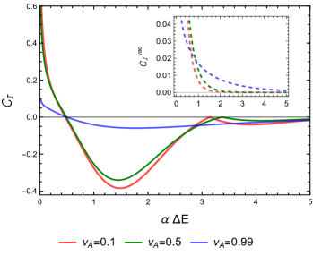
Figure 11: In $(1+3)$ dimensions for perpendicular motion of the detectors the integral $\mathcal{C}_{\mathcal{I}}$ signifying the concurrence is plotted as a function of $\alpha\,\Delta E$ for different fixed values of $v_{A}$. In this plot we have considered the distribution function $f(\omega_{k})=C\,\omega_{k}\,e^{-\alpha\omega_{k}}$ for the singly excited background field state. Here the velocity of detector $B$ is fixed at $v_{B}=0.55$ and the other parameter is $r_{0}/\alpha=1$. These curves assert that entanglement harvesting from single particle field state is possible in the low $\alpha\,\Delta E$ regimes. The inner plot correspond to $\mathcal{C}_{\mathcal{I}}^{vac}$, the concurrence, if the detectors were interacting with the field vacuum. Similar nature is also obtained for $r_{0}/\alpha=0.5$ case.

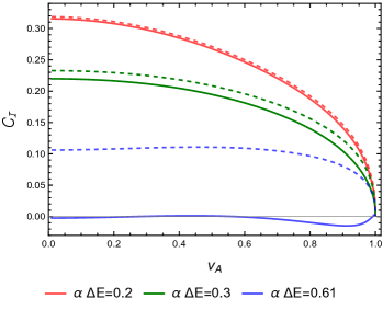
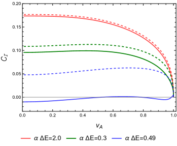
Figure 12: In $(1+3)$ dimensions for the detectors’ perpendicular motion the integral $\mathcal{C}_{\mathcal{I}}$, signifying the concurrence, is plotted as a function of $v_{A}$. The upper and the lower plots respectively correspond to $r_{0}/\alpha=0.5$ and $r_{0}/\alpha=1$. In both of these plots we have considered the distribution function $f(\omega_{k})=C\,\omega_{k}\,e^{-\alpha\omega_{k}}$ for the singly excited background field state. Here the velocity of detector $B$ is fixed at $v_{B}=0.55$. From these plots it is evident that with decreasing $\alpha\,\Delta E$ and $r_{0}/\alpha$ the concurrence increases. The solid lines denote the contributions from $\mathcal{C}_{\mathcal{I}}$, while the dashed lines denote $\mathcal{C}_{\mathcal{I}}^{vac}$.

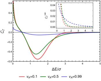
Figure 13: In $(1+3)$ dimensions for perpendicular motion of the detectors the integral $\mathcal{C}_{\mathcal{I}}$ signifying the concurrence is plotted as a function of $\Delta E/\sigma$ for different fixed values of $v_{A}$. In this plot we have considered the distribution function $f(\omega_{k})=C\,\omega_{k}~{}e^{-(\omega_{k}-\omega_{0})^{2}/2\sigma^{2}}$ for the singly excited background field state. Here the velocity of detector $B$ is fixed at $v_{B}=0.55$ and the other fixed parameters are $r_{0}\sigma=1$ and $\omega_{0}/\sigma=0.5$. Here also one can observed that entanglement harvesting from single particle field state is possible in the low $\Delta E/\sigma$ regimes. The inner plot correspond to $\mathcal{C}_{\mathcal{I}}^{vac}$, the concurrence, if the detectors were interacting with the field vacuum. Similar nature is also obtained for $r_{0}\sigma=0.5$ case.

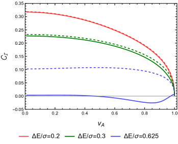
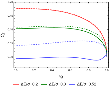
Figure 14: In $(1+3)$ dimensions for the detectors in perpendicular inertial motion, the integral $\mathcal{C}_{\mathcal{I}}$ signifying the concurrence is plotted as a function of $v_{A}$. The upper and the lower plots respectively correspond to $r_{0}/\sigma=0.5$ and $r_{0}/\sigma=1$. In both of these plots we have considered the distribution function $f(\omega_{k})=C~{}\omega_{k}~{}e^{-(\omega_{k}-\omega_{0})^{2}/2\sigma^{2}}$. Here the velocity of detector $B$ is fixed at $v_{B}=0.55$, and the other fixed parameter is $\omega_{0}/\sigma=0.5$. From these plots it is evident that with decreasing $\Delta E/\sigma$ and $r_{0}\,\sigma$ the concurrence increases. The solid lines denote the contributions from $\mathcal{C}_{\mathcal{I}}$, while the dashed lines denote $\mathcal{C}_{\mathcal{I}}^{vac}$.

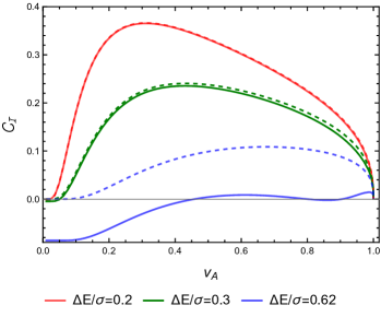
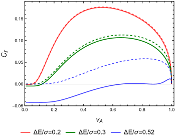
Figure 15: In $(1+3)$ dimensions the integral $\mathcal{C}_{\mathcal{I}}$ signifying the concurrence is plotted as a function of $v_{A}$ for $v_{B}=0$. The upper and the lower plots respectively correspond to $r_{0}\,\sigma=0.5$ and $r_{0}\,\sigma=1$, and these plots are the same for both parallel and perpendicular motions (see Eq. (43), and we have also checked this by plotting for the parallel and perpendicular cases). In both of these plots we have considered the distribution function $f(\omega_{k})=C~{}\omega_{k}~{}e^{-(\omega_{k}-\omega_{0})^{2}/2\sigma^{2}}$ for the singly excited background field state. It should be mentioned that with the exponential decaying distribution function also one gets similar plots with the same characteristics. Here the other fixed parameter is $\omega_{0}/\sigma=0.5$. From these plots it is evident that with decreasing $\Delta E/\sigma$ and $r_{0}\,\sigma$ the concurrence increases. The dashed lines denote the contributions from $\mathcal{C}_{\mathcal{I}}^{vac}$, while the solid lines denote $\mathcal{C}_{\mathcal{I}}$.

1

The plots from Figs. 11 and 13 of $\mathcal{C}_{\mathcal{I}}$ with respect to the transition energy $\Delta E$ in this perpendicular case represent nature similar to the parallel case (see Fig. 7 and 9). From these figures we observe that with increasing detector transition energy $\Delta E$ the harvesting decreases (only when $\mathcal{C}_{\mathcal{I}}$ is positive). In Fig. 12 and 14 we have plotted $\mathcal{C}_{\mathcal{I}}$ as functions of $v_{A}$ for fixed $v_{B}\neq 0$. We have also plotted the quantity $\mathcal{C}_{\mathcal{I}}^{vac}=\left|\mathcal{I}_{\varepsilon}\right|$ in these figures, which denotes the concurrence if the detectors were interacting with the field vacuum rather than the non-vacuum state. From these plots one can observe that entanglement harvesting from the single particle excited state is suppressed compared to the vacuum fluctuations. Here also, one can observe that in the limit of $v_{A}\to 1$, the quantity $\left|\mathcal{I}_{\varepsilon}\right|$ vanishes, leading to a vanishing concurrence, and this feature is evident in these figures. When the $\Delta E$ value is large the entanglement harvesting is happening in discrete intermediate and high velocity regimes. Like the parallel case here also entanglement harvesting decreases with increasing distance $r_{0}/\alpha$ between the perpendicular paths, and with increasing transition energy $\Delta E$. Here when the two detectors are in perpendicular inertial motion in $(1+3)$ dimensions the integral $\mathcal{I}_{\varepsilon_{R}}^{vac}$ does not vanish in the $v_{A}\to v_{B}$ limit unlike the parallel case. However, its expression in the $v_{B}\to 0$ limit is the same as the parallel case. We also observe that in the $v_{B}=0$ situation (plots corresponding to this situation are given in Fig. 15) the plots are the same as the parallel case (done in Koga et al. (2018), where one detector is taken to be stationary). While for $v_{B}\neq 0$ they are much different.

V Discussion

In the literature, most of the entanglement harvesting-related works, up to our knowledge, consider the detectors interacting with the field vacuum. However, in nature, one cannot expect that the background field will always be in a vacuum state. Then, the consideration of non-vacuum field states in understanding entanglement harvesting becomes essential from the practical point of view. The present work has considered single-particle background field excitations to investigate the entanglement harvesting between inertial Unruh-DeWitt detectors in $(1+1)$ and $(1+3)$ dimensions. Choice of single particle state is motivated from the earlier work Lochan and Padmanabhan (2015), and to build an analytically simple, tractable model. We have presented a thorough formulation for understanding entanglement harvesting from non-vacuum field states. Our main observation is that in both $(1+1)$ and $(1+3)$ dimensions, the entanglement harvested due to the single-particle background fluctuations is reduced compared to the vacuum fluctuations. The transition probability for inertial detectors interacting with the non-vacuum field state is non-zero and non-trivial (see Figs. 1, 2, 5, and 6). This non-zero transition probability is expected even if the detectors are inertial as they interact with non-vacuum field states. We also observed, both in $(1+1)$ and $(1+3)$ dimensions with detectors in parallel motion, that two detectors with the same velocity ($v_{A}=v_{B}$) do not harvest any entanglement among themselves when interacting with the single particle field state. This phenomenon was true even when the detectors interacted with the field vacuum. However, a similar situation with detectors in perpendicular inertial motion in $(1+3)$ dimensions is not observed. One observes increasing entanglement harvesting with decreasing detector transition energy in both these dimensions, for parallel and perpendicular motions, and the considered system parameters. In particular, in $(1+1)$ dimensions, there is visible occurrence of entanglement harvesting in low detector transition energy and high-velocity regimes (see Figs. 3 and 4). While in $(1+3)$ dimensions (both with detectors in parallel and perpendicular motion), one notices that entanglement harvesting stops when the velocity of detector $A$ approaches the velocity of light, i.e., when $v_{A}\to 1$ (see Figs. 8, 10, 12, 14, and 15). In $(1+3)$ dimensions the entanglement harvesting decreases with increasing perpendicular distance ($r_{0}$) between the two detectors.

We want to provide a few final comments, which are as follows. First, we emphasize that entanglement harvesting is possible only when $|\mathcal{I}_{\epsilon}|^{2}>\mathcal{I}_{A}\mathcal{I}_{B}$. The nonnegative measure of $\mathcal{C}_{\mathcal{I}}=|\mathcal{I}_{\epsilon}|-\sqrt{\mathcal{I}_{A}\mathcal{I}_{B}}$ quantifies the harvested entanglement. Interestingly the local terms $\mathcal{I}_{j}$ (with $j$ being either $A$ or $B$) denote individual detector transition probabilities. These terms have a vanishing contribution to inertial detectors interacting with the vacuum background scalar field. While for the background field in any excited state, these local terms for the similar detector motion are finite and nonzero. Therefore, the harvesting from the nonvacuum states is always expected to be lesser compared to the field vacuum if the entangling term $\mathcal{I}_{\epsilon}$ does not change much. In our current work, we found that this is indeed the case with single-particle excited states, as the entangling term $\mathcal{I}_{\epsilon}$ remains the same for the vacuum and nonvacuum field states.

Furthermore, we found some additional distinct features with the single-particle excited states compared to the vacuum field state. For example, for two inertial detectors moving at different velocities, entanglement harvesting from the field vacuum always seems possible as one varies the detector transition energy $\Delta E$. While the same is not true from the single-particle excited state as one can perceive ranges of no-harvesting in $\Delta E$. One observes this phenomenon in both $(1+1)$ and $(1+3)$ dimensions and for parallel and perpendicular cases. In this regard, see the plots of concurrence as a function of $\Delta E$ in Figs. 3, 4, 7, 9, 11, and 13. When examining the results with a varying velocity $v_{A}$ of the detector $A$, one may point out a similarly interesting distinguishing feature in the perpendicular motion case. In this scenario, one can observe discrete regions of entanglement harvesting in $v_{A}$ from the single-particle field states for larger detector transition energies. In comparison, in similar scenarios, entanglement harvesting from the vacuum is possible in the whole range $0<v_{A}<1$, see Figs. 12 and 14. These specific observations provide additional distinctions between the vacuum and single-particle entanglement harvesting cases other than the expected diminishing phenomenon observed for the latter case. Finally, one should notice that in nature, it is not guaranteed that the background field state will be in a vacuum. In fact, it is natural to believe that the fields will be in some excited state due to the presence of various constituents. Then, these specific features of harvesting shall provide some valuable distinctions of identification. Moreover, for the physical realization of entanglement harvesting from the single-particle field state, there is a restriction in the range of system parameters (prominently visible in $\Delta E$), unlike the vacuum. Therefore, contrary to the vacuum case, to observe the entanglement harvesting, one needs to construct a detector such that the transition energy must live within the allowed range of values.

Secondly, we shall like to emphasize that the nature of the individual detector transition probabilities $\mathcal{I}_{j}$ alters considerably depending on the motion of the detectors. For instance, inertial detectors have vanishing transition probabilities for interactions with the field vacuum. In contrast, the non-inertial detectors have non-vanishing contributions, which results in the Unruh effect for uniform linear acceleration. Therefore, the scenarios with non-inertial detectors demand an extensive and detailed investigation, and it is difficult to comment on these scenarios just by studying the inertial case. Nevertheless, entanglement harvesting from the non-vacuum field states with non-inertial detectors (see Refs. Koga et al. (2019); Barman and Majhi (2021); Barman et al. (2021a)) remains an interesting arena to venture further. In this regard, we believe the cases of charged detectors in circular trajectories Bell and Leinaas (1983, 1987); Akhmedov and Singleton (2007a, b) compels great enthusiasm as these systems open the avenue to realize many theoretical predictions physically.

We believe this work opens up a new avenue to understanding the nature of entanglement harvesting from non-vacuum field states. The immediate direction to look further, discussed in the previous paragraph and which we are currently working on, is entanglement harvesting from these non-vacuum field states with non-inertial detectors. In particular, some of our preliminary observations, corresponding to the uniformly accelerated linear motion of the detectors, are as follows. The excess contribution due to the non-vacuum fluctuations in the individual detector transition probability $\mathcal{I}_{j}$ is finite for detectors with infinite switching. Thus the relevant transition rate, coming from this contribution, over infinite time vanishes. In comparison, one observes that the same contribution $\mathcal{I}_{j}$ due to the vacuum fluctuation has a Dirac delta zero multiplying factor (see the transition probabilities of non-inertial Unruh-DeWitt detectors from Koga et al. (2019); Barman and Majhi (2021); Barman et al. (2021a)), which results in a finite transition rate for infinite time. Therefore, in concurrence per unit time, the different effects of vacuum and non-vacuum fluctuations will not be evident. We have considered detectors with finite time switching functions to circumvent this inconvenience, which provides finite transition probabilities. In future work, we wish to communicate the progress in this direction and with detectors in a circular motion. Our endeavor also includes investigating and comparing entangled atoms’ transition probability characteristics with the so-called Unruh effect of the accelerated observers for detectors interacting with a non-vacuum background field state.

Appendix A Normalized distribution functions for singly excited states

A.1 In $(1+1)$ dimensions

One may consider qualitatively different distribution functions $f(\omega_{k})$ (see Lochan and Padmanabhan (2015)). In $(1+1)$ dimensions a few examples follow, and we also provide their respective normalization constants. It should be noted that to evaluate the normalization constant in $f(\omega_{k})$, here one has to use the $(1+1)$ dimensional form of the normalization condition (10).

A.1.1 Exponential damping, $f(\omega_{k})=C\,\omega_{k}\,e^{-\alpha\omega_{k}}$

In this case the distribution function is of the form $f(\omega_{k})=C\,\omega_{k}\,e^{-\alpha\omega_{k}}$. Using the normalization condition (10) of $f(\omega_{k})$ for $(1+1)$ dimensions one can find out the value of the constant $C$ as $C=2\,\sqrt{2\pi}\,\alpha$.

A.1.2 Gaussian distribution, $f(\omega_{k})=C\,\omega_{k}\,e^{-(\omega_{k}-\omega_{0})^{2}/2\sigma^{2}}$

In this case the distribution function is of the form $f(\omega_{k})=C\,\omega_{k}\,e^{-(\omega_{k}-\omega_{0})^{2}/2\sigma^{2}}$. Using the normalization condition (10) of $f(\omega_{k})$ for $(1+1)$ dimensions one can find out the value of the constant $C$ here, as $C=\left\{4\sqrt{\pi}/\left[\omega_{0}\,\sigma\left(2-Q\left(-1/2,\omega_{0}^{2}/\sigma^{2}\right)\right)\right]\right\}^{1/2}$. Here $Q\left(a,z\right)$ denotes the Regularized Gamma Function.

A.2 In $(1+3)$ dimensions

In $(1+3)$ dimensions also one may consider similar distribution functions $f(\omega_{k})$. However, here one has to use the $(1+3)$ dimensional form of the normalization condition (10) to find out the respective normalization constants. Naturally the normalization constants $C$ obtained here will be different than the ones obtained for $(1+1)$ dimensional case.

A.2.1 Exponential damping, $f(\omega_{k})=C\,\omega_{k}\,e^{-\alpha\omega_{k}}$

Like the $(1+1)$ dimensional case here also we consider the same exponentially damping distribution function

$$f(\omega_{k})=C~{}\omega_{k}~{}e^{-\alpha\omega_{k}}~{}.$$ (56)

However, here the normalization constant $C$ is obtained from Eq. (10) by putting $d=3$, which corresponds to three spatial dimensions of our present case. Then this constant $C$ is given by $C=4\pi\alpha^{2}\,\sqrt{2/3}~{}$.

A.2.2 Gaussian distribution, $f(\omega_{k})=C\,\omega_{k}\,e^{-(\omega_{k}-\omega_{0})^{2}/2\sigma^{2}}$

We consider the Gaussian distribution function for a singly excited state in $(1+3)$ dimensions as

$$f(\omega_{k})=C~{}\omega_{k}~{}e^{-(\omega_{k}-\omega_{0})^{2}/2\sigma^{2}}.$$ (57)

Here also one has to use the normalization condition (10) with $d=3$ to evaluate the value of the normalization constant $C$, which is given by

$$C = 4\pi\Big{/}\bigg{\{}\sqrt{\pi}\omega_{0}\left(3\sigma^{2}+2\omega_{0}^{2}\right)\sigma\left(\textup{Erf}\left(\frac{\omega_{0}}{\sigma}\right)+1\right)$$ (58)

$$~{}~{}~{}~{}~{}~{}~{}~{}~{}~{}~{}~{}~{}~{}+2\sigma^{2}e^{-\frac{\omega_{0}^{2}}{\sigma^{2}}}\left(\sigma^{2}+\omega_{0}^{2}\right)\bigg{\}}^{1/2}~{},$$

where, $\textup{Erf}(z)$ denotes the error function.

Appendix B Evaluations of the integrals in $(1+1)$ dimensions

In this section of the Appendix we provide an explicit derivation of the integral $\mathcal{I}_{\varepsilon_{R}}^{vac}$. In particular, we shall be obtaining its expression as provided in Eq. (III.2) for two inertial detectors in $(1+1)$ dimensions. In this regard we consider the form of the integral from Eq. (17) with the consideration that $T_{j}=t_{j}$ are now the Minkowski times. Then this integral becomes

$$\mathcal{I}_{\varepsilon_{R}}^{vac} = \frac{1}{\gamma_{A}\gamma_{B}}\int_{-\infty}^{\infty}\frac{dk}{4\pi\omega_{k}}\,\int_{-\infty}^{\infty}dt_{A}\int_{-\infty}^{\infty}dt_{B}\,\theta(t_{A}-t_{B})$$

$$\times e^{i\Delta E(t_{B}/\gamma_{B}+t_{A}/\gamma_{A})}\,\Big{[}e^{-i(\omega_{k}-k\,v_{B})\,t_{B}+i(\omega_{k}-k\,v_{A})\,t_{A}}$$

$$~{}~{}-e^{i(\omega_{k}-k\,v_{B})\,t_{B}-i(\omega_{k}-k\,v_{A})\,t_{A}}\Big{]}$$

$$= \frac{1}{\gamma_{A}\gamma_{B}}\int_{-\infty}^{\infty}\frac{dk}{4\pi\omega_{k}}\,\int_{-\infty}^{\infty}dt_{A}\int_{-\infty}^{t_{A}}dt_{B}$$

$$\times e^{i\Delta E(t_{B}/\gamma_{B}+t_{A}/\gamma_{A})}\,\Big{[}e^{-i(\omega_{k}-k\,v_{B})\,t_{B}+i(\omega_{k}-k\,v_{A})\,t_{A}}$$

$$~{}~{}-e^{i(\omega_{k}-k\,v_{B})\,t_{B}-i(\omega_{k}-k\,v_{A})\,t_{A}}\Big{]}$$

$$= \frac{i}{\gamma_{A}\gamma_{B}}\int_{-\infty}^{\infty}\frac{dk}{4\pi\omega_{k}}\,\int_{-\infty}^{\infty}dt_{A}\,e^{i\Delta E\,t_{A}(1/\gamma_{B}+1/\gamma_{A})}\,$$

$$\times \Bigg{[}\frac{e^{-i\{k\,(v_{A}-v_{B})+i\,\epsilon\}\,t_{A}}}{\omega_{k}-k\,v_{B}-\Delta{E}/\gamma_{B}}+\frac{e^{i\,k\{(v_{A}-v_{B})-i\,\epsilon\}\,t_{A}}}{\omega_{k}-k\,v_{B}+\Delta{E}/\gamma_{B}}\Bigg{]}\,,$$

where one can observe that a $e^{\epsilon\,t_{B}}$ regulator, with positive small $\epsilon$, was introduced to make the $t_{B}$ integral convergent in the lower limit of negative infinity. The actual integral is obtained in the limit of $\epsilon\to 0$. After performing the $t_{A}$ integration now one can obtain

$$\mathcal{I}_{\varepsilon_{R}}^{vac} = \frac{i}{\gamma_{A}\gamma_{B}}\int_{-\infty}^{\infty}\frac{dk}{2\omega_{k}}\,\Bigg{[}\tfrac{\delta\left[k(v_{A}-v_{B})-\Delta{E}\left(\frac{1}{\gamma_{A}}+\frac{1}{\gamma_{B}}\right)\right]}{\omega_{k}-k\,v_{B}-\Delta{E}/\gamma_{B}}$$

$$+~{}\tfrac{\delta\left[k(v_{A}-v_{B})+\Delta{E}\left(\frac{1}{\gamma_{A}}+\frac{1}{\gamma_{B}}\right)\right]}{\omega_{k}-k\,v_{B}+\Delta{E}/\gamma_{B}}\Bigg{]}\,.$$ (60)

This expression is the same as the one presented in Eq. (III.2).

Appendix C Evaluations of the integrals in $(1+3)$ dimensions for detectors in parallel motion

C.1 Explicit evaluation of $\mathcal{I}_{A}$

Here we consider evaluating the necessary integrals for entanglement harvesting for two detectors in parallel inertial motion in $(1+3)$ dimensions. To derive the expression of the quantity $\mathcal{I}_{A}$ corresponding to detector $A$ we consider the trajectory from Eq. (32) and the $\mathcal{A}(\Delta E)$ part of it becomes

$$\mathcal{A}(\Delta E) = \int_{-\infty}^{\infty}d\tau_{A}e^{i\Delta E\tau_{A}}\Phi_{\mathrm{eff}}(x)$$ (61)

$$= \int_{-\infty}^{\infty}d\tau_{A}e^{i\Delta E\tau_{A}}\int_{0}^{\pi}\int_{0}^{\infty}\frac{2\pi\sin\theta\omega_{k}^{2}d\omega_{k}d\theta}{(2\pi)^{3}}$$

$$~{}~{}~{}~{}~{}~{}~{}~{}~{}~{}~{}~{}~{}~{}~{}~{}\times\frac{f(\omega_{k})}{2\omega_{k}}~{}e^{-i\omega_{k}\gamma_{A}\tau_{A}+i\omega_{k}\gamma_{A}v\tau_{A}\cos\theta}$$

$$= -\frac{i}{2(2\pi)^{2}\gamma_{A}v_{A}}\int_{0}^{\infty}d\omega_{k}f(\omega_{k})\int_{-\infty}^{\infty}\frac{d\tau_{A}}{\tau_{A}}$$

$$~{}~{}\times~{}[e^{i\tau_{A}(\Delta E-\omega_{k}/D_{A})}-e^{i\tau_{A}(\Delta E-\omega_{k}D_{A})}]\,,$$

where $D_{j}=\sqrt{(1+v_{j})/(1-v_{j})}$ and $\theta$-integration is done to obtain the final result. Now it is known that

$$\int_{-\infty}^{\infty}d\tau\frac{e^{i\tau\alpha}}{\tau} = \int_{-\infty}^{\infty}d\tau\frac{\cos{\tau\alpha}}{\tau}+i\int_{-\infty}^{\infty}d\tau\frac{\sin{\tau\alpha}}{\tau}$$ (62)

$$= i\pi\,\text{sgn}(\alpha)$$

where $\operatorname{sgn}(\alpha)$ is $\pm 1$ depending on positive or negative sign of the $\alpha$, or $zero$ for $\alpha=0$. Thus the expression of (61) is non-zero only when, $1/D_{A}\leq\omega_{k}/\Delta E\leq D_{A}$, i.e., when $(\Delta E-\omega_{k}/D_{A})>0$ with $(\Delta E-\omega_{k}D_{A})<0$. Therefore (61) becomes

$$\mathcal{A}(\Delta E)=\frac{1}{4\pi\gamma_{A}v_{A}}\int_{\Delta E/D_{A}}^{D_{A}\Delta E}d\omega_{k}f(\omega_{k})~{}.$$ (63)

Similarly one can check that

$$\mathcal{B}(\Delta E) = \int_{-\infty}^{\infty}d\tau_{A}\,e^{i\Delta E\,\tau_{A}}\Phi^{\star}_{\mathrm{eff}}(x)$$

$$= -\frac{i}{2(2\pi)^{2}\gamma_{A}v_{A}}\int d\omega_{k}f(\omega_{k})[i\pi-i\pi]$$

$$= 0~{}.$$ (64)

C.2 Explicit evaluation of $\mathcal{I}_{B}$

The quantity $\mathcal{A}(\Delta E)$ for detector $B$ from Eq. (20a) can be evaluated as

$$\mathcal{A}(\Delta E)$$

$$=\int_{-\infty}^{\infty}d\tau_{B}e^{i\Delta E\tau_{B}}\Phi_{\mathrm{eff}}(x_{B})$$

$$=\int_{-\infty}^{\infty}d\tau_{B}e^{i\Delta E\tau_{B}}\int_{0}^{2\pi}\int_{0}^{\pi}\int_{0}^{\infty}\frac{d\phi\sin\theta\omega_{k}^{2}d\omega_{k}d\theta}{(2\pi)^{3}}\frac{f(\omega_{k})}{2\omega_{k}}$$

$$~{}~{}~{}~{}\times e^{-i\omega_{k}\gamma_{B}\tau_{B}+i\omega_{k}\sin\theta(x_{0}\cos\phi+y_{0}\sin\phi)+i\omega_{k}v_{B}\gamma_{B}\tau_{B}\cos\theta}$$

$$=\int_{-\infty}^{\infty}d\tau_{B}e^{i\Delta E\tau_{B}}\int_{0}^{\pi}\int_{0}^{\infty}\frac{\sin\theta d\theta\omega_{k}d\omega_{k}}{(2\pi)^{2}}\frac{f(\omega_{k})}{2}$$

$$~{}~{}~{}~{}~{}~{}~{}~{}~{}~{}~{}~{}~{}~{}~{}\times e^{-i\omega_{k}\gamma_{B}\tau_{B}(1-v_{B}\cos\theta)}J_{0}(\omega_{k}r_{0}\sin\theta)$$

$$=\int_{-1}^{1}du\int_{0}^{\infty}\frac{\omega_{k}d\omega_{k}}{(2\pi)}\frac{f(\omega_{k})}{2}\delta(\Delta E-\omega_{k}\gamma_{B}(1-v_{B}u))$$

$$~{}~{}~{}~{}~{}~{}~{}~{}~{}\times J_{0}(\omega_{k}r_{0}\sqrt{1-u^{2}})$$

$$=\int_{-1}^{1}\frac{du}{4\pi}\frac{\Delta E~{}f\left(\frac{\Delta E}{\gamma_{B}(1-v_{B}u)}\right)}{\{\gamma_{B}(1-v_{B}u)\}^{2}}J_{0}\left(\tfrac{r_{0}\Delta E\sqrt{1-u^{2}}}{\gamma_{B}(1-v_{B}u)}\right),$$ (65)

where after the third equality we have defined $u=\cos\theta$. We can evaluate the integration over $u$ in (C.2) numerically using the expressions of $f(\omega_{k})$ given in (56) and (57), with the appropriate forms of the normalization constant $C$ separately in $(1+1)$ and $(1+3)$ dimensions.

C.3 Explicit evaluation of $\mathcal{I}_{\varepsilon}$

C.3.1 Considering the expression of the Green’s function in position space

Here we consider the position space representation of the Green’s function appearing in the expression of the integral

$$\mathcal{I}_{\varepsilon_{R}}^{vac}=-i\int_{-\infty}^{\infty}d\tau_{B}\int_{-\infty}^{\infty}d\tau_{A}e^{i\Delta E(\tau_{A}+\tau_{B})}G_{R}\left(X_{A},X_{B}\right).$$ (66)

The retarded Green function $G_{R}\left(X_{A},X_{B}\right)$ corresponding to a massless, minimally coupled free scalar field in the Minkowski spacetime is

$$G_{R}\left(X_{A},X_{B}\right) = -\frac{1}{2\pi}~{}\Theta\left(t_{A}-t_{B}\right)$$

$$\times\,\delta\left(\left(t_{A}-t_{B}\right)^{2}-\left|\bm{x}_{A}-\bm{x}_{B}\right|^{2}\right)$$ (67)

$$= -\frac{1}{2\pi}\Theta\left(t_{A}-t_{B}\right)\delta(g(t_{A},t_{B}))~{}.$$

For two detectors moving in parallel inertial trajectories (see Eq. (32) and (33)) in $(1+3)$ dimensions the argument of the Dirac delta distribution becomes zero when

$$g(t_{A},t_{B}) = {A}^{2}(1-v_{A}^{2})+t_{B}^{2}(1-v_{B}^{2})-2t_{A}t_{B}(1-v_{A}v_{B})-r_{0}^{2}$$

$$= 0~{}.$$ (68)

This equation has solutions for $t_{B}$ as

$$t_{B}=\gamma_{B}^{2}(t_{A}(1-v_{A}v_{B})\pm u(t_{A}))\equiv t_{\pm}$$ (69)

where,

$$u(t_{A})=\sqrt{t_{A}^{2}(v_{A}-v_{B})^{2}+r_{0}^{2}(1-v_{B}^{2})}.$$ (70)

Now, with the general condition $0\leq v_{j}\leq 1$, one can check that

$$t_{+}>t_{A}~{},$$

$$t_{-}<t_{A}~{}.$$ (71)

Then using the property of Dirac delta functions, we have

$$\delta(g(t_{A},t_{B})) = \left[\frac{\delta(t_{B}-t_{+})}{|g^{\prime}(t_{A},t_{B})|_{t_{B}=t_{+}}}+\frac{\delta(t_{B}-t_{-})}{|g^{\prime}(t_{A},t_{B})|_{t_{B}=t_{-}}}\right]$$ (72)

$$= \frac{1}{2u(t_{A})}[\delta(t_{B}-t_{+})+\delta(t_{B}-t_{-})]~{}~{}$$

Therefore one may express the integral of Eq. (66) as

$$\mathcal{I}_{\varepsilon_{R}}^{vac} = \frac{-i}{2\pi}\int_{-\infty}^{\infty}{\frac{dt_{A}}{\gamma_{A}}}\int_{-\infty}^{t_{A}}{\frac{dt_{B}}{\gamma_{B}}}e^{i\Delta{E}\big{(}\frac{t_{A}}{\gamma_{A}}+\frac{t_{B}}{\gamma_{B}}\big{)}}\delta(g(t_{A},t_{B}))$$

$$= \frac{-i}{4\pi}\int_{-\infty}^{\infty}{\frac{dt_{A}}{\gamma_{A}\gamma_{B}~{}u(t_{A})}}e^{i\Delta{E}\left(\frac{t_{A}}{\gamma_{A}}+\gamma_{B}(t_{A}(1-v_{A}v_{B})-u(t_{A}))\right)}$$

$$= \frac{-i}{2\pi}\int_{0}^{\infty}\scalebox{0.95}{$\frac{dt_{A}e^{-i\Delta{E}\gamma_{B}u(t_{A})}}{\gamma_{A}\gamma_{B}\,u(t_{A})}\cos$}\scalebox{0.85}{$\left(\Delta{E}t_{A}\left(\frac{1}{\gamma_{A}}+\gamma_{B}(1-v_{A}v_{B})\right)\right)$}~{}.$$

Now expanding the exponential in (C.3.1) in terms of $sin$ and $cos$ functions and by comparing with (IV.1.2), we can recognise

$$a = \frac{r_{0}}{\gamma_{B}|v_{A}-v_{B}|};~{}~{}\varrho=\gamma_{B}|v_{A}-v_{B}|\Delta{E};$$

$$\beta = \Delta{E}\left(\frac{1}{\gamma_{A}}+\gamma_{B}(1-v_{A}v_{B})\right);$$ (74)

as we know $0\leq v_{j}\leq 1$, this satisfies the criteria for (IV.1.2), $i.e.$,

$$\beta>\varrho~{}\text{or,~{}}\left(\frac{1}{\gamma_{A}}+\gamma_{B}(1-v_{A}v_{B})\right)>\gamma_{B}|v_{A}-v_{B}|$$

$$\text{or,~{}~{}}\frac{1}{\gamma_{A}(1-v_{A}v_{B})}+\gamma_{B}>\gamma_{B}|v_{rel}|.$$ (75)

Thus $\beta>\varrho>0$ is satisfies as the relative velocity ($v_{rel}$) between the detectors is always less than $one$. Therefore, from (C.3.1), we obtain

$$\mathcal{I}_{\varepsilon_{R}}^{vac} = \frac{-i}{2\pi\gamma_{A}\gamma_{B}|v_{A}-v_{B}|}$$

$$\times K_{0}\left(\tfrac{r_{0}\Delta{E}}{\gamma_{B}}\sqrt{\left(\tfrac{\frac{1}{\gamma_{A}}+\gamma_{B}(1-v_{A}v_{B})}{v_{A}-v_{B}}\right)^{2}-\gamma_{B}^{2}}\right)~{}.$$

If $v_{A}=v_{B}$ then from (69) and (70), we obtain $u(t_{A})$ is $t_{A}$ independent and $t_{-}=t_{A}-r_{0}\gamma_{B}$. Therefore, the $t_{A}$-integration after the second last line of (C.3.1) gives a delta function of form $\delta\left(\Delta{E}\left(1/\gamma_{A}+1/\gamma_{B}\right)\right)$. This is always $zero$ for $v_{A}=v_{B}$, as both $\gamma_{A}$ and $\Delta{E}$ are always positive. One can also simply take the limit $(v_{A}-v_{B})\to 0$ and observe that this quantity readily vanishes from Eq. (C.3.1).

C.3.2 Considering the expression of the Green’s function in momentum space

On the other hand, considering the expression of the Green’s function in momentum space on can express the integral $\mathcal{I}_{\varepsilon_{R}}^{vac}$ from Eq. (66) as

$$\mathcal{I}_{\varepsilon_{R}}^{vac} = -\int_{-\infty}^{\infty}d\tau_{A}\int_{-\infty}^{\infty}d\tau_{B}~{}e^{i\Delta{E}(\tau_{A}+\tau_{B})}\theta(\gamma_{A}\tau_{A}-\gamma_{B}\tau_{B})$$ (77)

$$~{}~{}~{}\times\int_{0}^{\pi}\sin\theta d\theta\int_{0}^{\infty}\frac{\omega_{k}d\omega_{k}}{2(2\pi)^{2}}\Big{[}e^{-i\omega_{k}(\gamma_{A}\tau_{A}-\gamma_{B}\tau_{B})}$$

$$~{}~{}~{}~{}~{}~{}~{}~{}\times e^{i\omega_{k}\sqrt{(\gamma_{A}\tau_{A}v_{A}-\gamma_{B}\tau_{B}v_{B})^{2}+r_{0}^{2}}\cos\theta}$$

$$-e^{i\omega_{k}(\gamma_{A}\tau_{A}-\gamma_{B}\tau_{B})-i\omega_{k}\sqrt{(\gamma_{A}\tau_{A}v_{A}-\gamma_{B}\tau_{B}v_{B})^{2}+r_{0}^{2}}\cos\theta}\Big{]}$$

$$= -\int_{-\infty}^{\infty}\int_{-\infty}^{\infty}\frac{dp~{}dq}{2v_{A}v_{B}^{\prime}\gamma_{A}\gamma_{B}}e^{i\Delta{E}(a_{1}p+a_{2}q)}\theta(a_{3}p-q)$$

$$\times\int_{-1}^{1}du\int_{0}^{\infty}\frac{\omega_{k}d\omega_{k}}{2(2\pi)^{2}}\Big{[}e^{-i\omega_{k}a_{4}(a_{3}p-q)+i\omega_{k}\sqrt{p^{2}+r_{0}^{2}}u}$$

$$~{}~{}~{}~{}~{}~{}~{}~{}~{}~{}~{}~{}-e^{i\omega_{k}a_{4}(a_{3}p-q)-i\omega_{k}\sqrt{p^{2}+r_{0}^{2}}u}\Big{]}\,.$$

As we have already discussed in sec. IV.1, here we defined a change of variables, $p=v_{A}\gamma_{A}\tau_{A}-v_{B}\gamma_{B}\tau_{B}$ and $q=v_{A}\gamma_{A}\tau_{A}+v_{B}\gamma_{B}\tau_{B}$. The Jacobian of the transform is given by $|J|=1/(2v_{A}v_{B}\gamma_{A}\gamma_{B})$. Under this transform the quantities $(\gamma_{A}\tau_{A}-\gamma_{B}\tau_{B})$ and $(\tau_{A}+\tau_{B})$, can be expressed as

$$\gamma_{A}\tau_{A}-\gamma_{B}\tau_{B}=\frac{p+q}{2v_{A}}-\frac{q-p}{2v_{B}}=\scalebox{1.1}{$\frac{p(v_{B}+v_{A})+q(v_{B}-v_{A})}{2v_{A}v_{B}}$}$$

$$~{}~{}~{}~{}~{}~{}=\frac{v_{A}-v_{B}}{2v_{A}v_{B}}\left(p\frac{v_{A}+v_{B}}{v_{A}-v_{B}}-q\right)=a_{4}(a_{3}p-q);$$

$$\tau_{A}+\tau_{B}=p\scalebox{1.1}{$\left(\frac{1}{2v_{A}\gamma_{A}}-\frac{1}{2v_{B}\gamma_{B}}\right)$}+q\scalebox{1.1}{$\left(\frac{1}{2v_{A}\gamma_{A}}+\frac{1}{2v_{B}\gamma_{B}}\right)$}$$

$$~{}~{}~{}~{}~{}~{}~{}~{}=a_{1}p+a_{2}q;$$ (78)

In Eq. (77) the step function provides the upper limit of $q$-integration, which is $a_{3}p$. After evaluating the $q$-integral, we obtain

$$\mathcal{I}_{\varepsilon_{R}}^{vac} = -\int_{-\infty}^{\infty}\frac{dp~{}e^{i\Delta{E}a_{1}p}}{2vv^{\prime}\gamma^{\prime}\gamma}\int_{-1}^{1}du\int_{0}^{\infty}\frac{\omega_{k}d\omega_{k}}{8\pi^{2}}$$

$$\times\,\Big{[}\frac{e^{i\Delta{E}a_{2}a_{3}p}}{i(\Delta{E}a_{2}+a_{4}\omega_{k})}\,e^{i\omega_{k}\sqrt{p^{2}+r_{0}^{2}}u}$$

$$-\frac{e^{i\Delta{E}a_{2}a_{3}p}}{i(\Delta{E}a_{2}-a_{4}\omega_{k})}e^{-i\omega_{k}\sqrt{p^{2}+r_{0}^{2}}u}\Big{]}~{}.$$ (79)

Then we perform the $u$-integral and after some re-arrangement we obtain

$$\mathcal{I}_{\varepsilon_{R}}^{vac} = \int_{-\infty}^{\infty}\frac{dp~{}e^{i\Delta{E}p(a_{1}+a_{2}a_{3})}}{16\pi^{2}vv^{\prime}\gamma^{\prime}\gamma\sqrt{p^{2}+r_{0}^{2}}}\Bigg{[}\int_{-\infty}^{\infty}\frac{d\omega_{k}~{}e^{i\omega_{k}\sqrt{p^{2}+r_{0}^{2}}}}{a_{4}\omega_{k}+a_{2}\Delta{E}}$$ (80)

$$~{}~{}~{}~{}~{}~{}~{}~{}~{}~{}+\int_{-\infty}^{\infty}\frac{d\omega_{k}~{}e^{i\omega_{k}\sqrt{p^{2}+r_{0}^{2}}}}{a_{4}\omega_{k}-a_{2}\Delta{E}}\Bigg{]}.$$

To evaluate the $\omega_{k}$-integration we change the integration variable to $a_{4}\omega_{k}\pm~{}a_{2}\Delta{E}$ for first and second integration, respectively. The integration limit remain unchanged as the quantities $a_{4},~{}a_{2}\Delta{E}$ are finite. Then we will use an identity from complex variable theory, that is

$$\int_{-\infty}^{\infty}{dx}\frac{e^{i\alpha x}}{x}=i\pi~{}\text{sgn}(\alpha)~{},$$ (81)

then the expression from (80) will become

$$\mathcal{I}_{\varepsilon_{R}}^{vac} = i\int_{-\infty}^{\infty}\tfrac{dp~{}e^{i\Delta{E}p(a_{1}+a_{2}a_{3})}}{8\pi v_{A}v_{B}\gamma_{A}\gamma_{B}a_{4}\sqrt{p^{2}+r_{0}^{2}}}~{}\cos\left(\tfrac{a_{2}\Delta{E}\sqrt{p^{2}+r_{0}^{2}}}{a_{4}}\right)$$ (82)

$$=i\int_{0}^{\infty}\tfrac{dp~{}\cos\left(\frac{a_{2}\Delta{E}}{a_{4}}\sqrt{p^{2}+r_{0}^{2}}\right)}{2\pi(v_{A}-v_{B})\gamma_{A}\gamma_{B}\sqrt{p^{2}+r_{0}^{2}}}\cos\left(\Delta{E}p(a_{1}+a_{2}a_{3})\right)$$

$$=\tfrac{i~{}K_{0}\left(r_{0}\Delta{E}\sqrt{\left(a_{1}+a_{2}a_{3}\right)^{2}-\left(a_{2}/a_{4}\right)^{2}}\right)}{2\pi(v_{A}-v_{B})\gamma_{A}\gamma_{B}}~{},$$

where we have used the integral representation from Eq. (IV.1.2).

In a manner similar to the previous case one can also express the integral $\mathcal{I}_{\varepsilon_{W}}^{vac}$ as

$$\mathcal{I}_{\varepsilon_{W}}^{vac} = -\int_{-\infty}^{\infty}d\tau_{A}\int_{-\infty}^{\infty}d\tau_{B}e^{i\Delta{E}(\tau_{A}+\tau_{B})}G_{W}(X_{A},X_{B})$$

$$= -\int_{-\infty}^{\infty}d\tau_{A}\int_{-\infty}^{\infty}d\tau_{B}e^{i\Delta{E}(\tau_{A}+\tau_{B})}\int_{0}^{\pi}\sin\theta\,d\theta$$

$$\times\int_{0}^{\infty}\frac{\omega_{k}d\omega_{k}}{2(2\pi)^{2}}\,e^{-i\omega_{k}(\gamma_{A}\tau_{A}-\gamma_{B}\tau_{B})}$$

$$\times~{}e^{i\omega_{k}\sqrt{(\gamma_{A}\tau_{A}v_{A}-\gamma_{B}\tau_{B}v_{B})^{2}+r_{0}^{2}}\cos\theta}~{}.$$ (83)

Using the previously mentioned coordinate transformation, related to Eq. (78), the quantity from Eq. (C.3.2) can be evaluated as

$$\mathcal{I}_{\varepsilon_{W}}^{vac} = -\int_{-\infty}^{\infty}\int_{-\infty}^{\infty}\frac{dp~{}dq~{}e^{i\Delta{E}(a_{1}p+a_{2}q)}}{2v_{A}v_{B}\gamma_{A}\gamma_{B}}\int_{0}^{\pi}\sin\theta d\theta$$

$$\times~{}\int_{0}^{\infty}\frac{\omega_{k}d\omega_{k}}{2(2\pi)^{2}}\,e^{-i\omega_{k}a_{4}(a_{3}p-q)+i\omega_{k}\sqrt{p^{2}+r_{0}^{2}}\cos\theta}$$

$$= -\int_{-1}^{1}du\int_{0}^{\infty}\frac{\omega_{k}d\omega_{k}}{8\pi^{2}}\int_{-\infty}^{\infty}\frac{dp~{}e^{i\Delta{E}a_{1}p}}{2v_{A}v_{B}\gamma_{A}\gamma_{B}}$$

$$\times~{}e^{-i\omega_{k}a_{3}a_{4}p+i\omega_{k}\sqrt{p^{2}+r_{0}^{2}}u}\int_{-\infty}^{\infty}dq~{}e^{i(a_{2}\Delta{E}+a_{4}\omega_{k})q}$$

$$= -\int_{-1}^{1}du\int_{0}^{\infty}\frac{\omega_{k}d\omega_{k}}{4\pi}\int_{-\infty}^{\infty}\frac{dp~{}}{2v_{A}v_{B}\gamma_{A}\gamma_{B}}e^{i\omega_{k}\sqrt{p^{2}+r_{0}^{2}}u}$$

$$\times~{}e^{ip(a_{1}\Delta{E}-a_{3}a_{4}\omega_{k})}~{}\delta(a_{2}\Delta{E}+a_{4}\omega_{k})$$

$$= 0~{}.$$ (84)

Appendix D Evaluations of the integrals in $(1+3)$ dimensions for detectors in perpendicular motion

D.1 Explicit evaluation of $\mathcal{I}_{A}$

We will evaluate $\mathcal{I}_{A}^{nv}$ for trajectory (44). In particular, the $\mathcal{A}(\Delta E)$ part of this quantity becomes

$$\mathcal{A}(\Delta E) = \int_{-\infty}^{\infty}{d\tau_{A}}e^{i\Delta E\tau_{A}}\phi_{eff}(x_{A})$$

$$= \int_{-\infty}^{\infty}{d\tau_{A}}e^{i\Delta E\tau_{A}}\int_{0}^{\infty}\frac{\omega_{k}d\omega_{k}}{2(2\pi)^{3}}\int_{0}^{\pi}\sin\theta d\theta\int_{0}^{2\pi}d\phi$$

$$~{}~{}~{}~{}~{}~{}~{}~{}~{}~{}~{}~{}~{}~{}~{}\times e^{-i\omega_{k}t_{A}+i\omega_{k}v_{A}t_{A}\sin\theta\cos\phi}f(\omega_{k})$$

$$= \int_{-\infty}^{\infty}{d\tau_{A}}e^{i\Delta E\tau_{A}}\int_{0}^{\infty}\frac{\omega_{k}d\omega_{k}}{2(2\pi)^{2}}\int_{-1}^{1}du~{}e^{-i\omega_{k}t_{A}}f(\omega_{k})$$

$$~{}~{}~{}~{}~{}~{}~{}~{}~{}~{}~{}~{}~{}~{}~{}~{}~{}~{}~{}~{}~{}~{}~{}~{}~{}\times J_{0}(|\omega_{k}v_{A}t_{A}\sqrt{1-u^{2}}|)$$

$$= \int_{-\infty}^{\infty}{\frac{dt_{A}}{\gamma}}e^{i\Delta Et_{A}/\gamma_{A}}\int_{0}^{\infty}\frac{\omega_{k}d\omega_{k}}{2(2\pi)^{2}}e^{-i\omega_{k}t_{A}}f(\omega_{k})$$

$$~{}~{}~{}~{}~{}~{}~{}~{}~{}~{}~{}~{}~{}~{}~{}~{}~{}~{}~{}~{}~{}~{}~{}~{}~{}~{}~{}~{}~{}\times~{}\frac{2\sin{\omega_{k}v_{A}t_{A}}}{\omega_{k}v_{A}t_{A}}$$ (85)

$$= \int_{0}^{\infty}\frac{d\omega_{k}~{}f(\omega_{k})}{i2(2\pi)^{2}v_{A}\gamma_{A}}\int_{-\infty}^{\infty}\frac{dt_{A}}{t_{A}}[e^{i(\Delta E-\frac{\omega_{k}}{D_{A}})t_{A}/\gamma_{A}}$$

$$~{}~{}~{}~{}~{}~{}~{}~{}~{}~{}~{}~{}~{}~{}~{}~{}~{}~{}~{}~{}~{}~{}~{}~{}~{}-e^{i(\Delta E-\omega_{k}D_{A})t_{A}/\gamma_{A}}]$$

$$= \int_{0}^{\infty}\frac{d\omega_{k}}{i2(2\pi)^{2}v_{A}\gamma_{A}}f(\omega_{k})i\pi[\text{sgn}(D_{A}\Delta E-\omega_{k})$$

$$~{}~{}~{}~{}~{}~{}~{}~{}~{}~{}~{}~{}~{}~{}~{}~{}~{}~{}~{}~{}~{}~{}~{}~{}~{}-\text{sgn}(\Delta E/D_{A}-\omega_{k})]$$

$$= \frac{1}{4\pi v_{A}\gamma_{A}}\int_{\Delta E/D_{A}}^{\Delta ED_{A}}d\omega_{k}\,f(\omega_{k})~{}.$$

As all other quantities in $\mathcal{I}_{A}$ are zero, one can express $\mathcal{I}_{A}=\left|\mathcal{A}(\Delta E)\right|^{2}$. This expression is same as the one from Eq. (63) for two detectors in parallel inertial motion in $(1+3)$ dimensions, as expected.

D.2 Explicit evaluation of $\mathcal{I}_{\varepsilon}$

Now let us evaluate $\mathcal{I}_{\varepsilon_{W}}^{vac}$ for two detectors in perpendicular inertial motions. For $t_{A}>t_{B}$, we have positive frequency Wightman function

$$G_{W} (X_{A},X_{B})$$ (86)

$$= -\frac{1}{4\pi^{2}}\frac{1}{(t_{A}-t_{B}-i\epsilon)^{2}-|\bm{x}_{A}-\bm{x}_{B}|^{2}}$$

$$= -\frac{1}{4\pi^{2}}\frac{1}{g(t_{A},t_{B})-i\epsilon}~{}.$$

No contribution for $t_{B}>t_{A}$, will be taken. Now, solving for $g(t_{A},t_{B})-i\epsilon=0$ gives, $t_{B}=\gamma_{B}^{2}(t_{A}\pm u(t_{A})(1+i\epsilon))=t_{\pm}(1\pm i\epsilon)$. We already know that $t_{B}=t_{+}>t_{A}$ and $t_{B}=t_{-}<t_{A}$. When $t_{A}>t_{B}$ satisfied, we have pole in the lower half of the complex $t_{B}$-plane. Thus

$$\mathcal{I}_{\varepsilon_{W}}^{vac} = -\int_{-\infty}^{\infty}\int_{-\infty}^{\infty}d\tau_{A}d\tau_{B}e^{i\Delta{E}(\tau_{A}+\tau_{B})}G_{W}(X_{A},X_{B})$$

$$= 0~{}.$$ (87)

References

- Fuentes-Schuller and Mann (2005) I. Fuentes-Schuller and R. B. Mann, Phys. Rev. Lett. 95, 120404 (2005), eprint arXiv:quant-ph/0410172.
- Reznik (2003) B. Reznik, Found. Phys. 33, 167 (2003), eprint arXiv:quant-ph/0212044.
- Lin and Hu (2010) S.-Y. Lin and B. Hu, Phys. Rev. D 81, 045019 (2010), eprint arXiv:0910.5858.
- Ball et al. (2006) J. L. Ball, I. Fuentes-Schuller, and F. P. Schuller, Phys. Lett. A 359, 550 (2006), eprint arXiv:quant-ph/0506113.
- Cliche and Kempf (2010) M. Cliche and A. Kempf, Phys. Rev. A 81, 012330 (2010), eprint arXiv:0908.3144.
- Martin-Martinez and Menicucci (2012) E. Martin-Martinez and N. C. Menicucci, Class. Quant. Grav. 29, 224003 (2012), eprint arXiv:1204.4918.
- Salton et al. (2015) G. Salton, R. B. Mann, and N. C. Menicucci, New J. Phys. 17, 035001 (2015), eprint arXiv:1408.1395.
- Martin-Martinez et al. (2016) E. Martin-Martinez, A. R. H. Smith, and D. R. Terno, Phys. Rev. D 93, 044001 (2016), eprint arXiv:1507.02688.
- Cai and Ren (2018) H. Cai and Z. Ren, Sci. Rep. 8, 11802 (2018).
- Menezes (2018) G. Menezes, Phys. Rev. D97, 085021 (2018), eprint arXiv:1712.07151.
- Menezes et al. (2017) G. Menezes, N. Svaiter, and C. Zarro, Phys. Rev. A 96, 062119 (2017), eprint arXiv:1709.08702.
- Zhou and Yu (2017) W. Zhou and H. Yu, Phys. Rev. D 96, 045018 (2017).
- Benatti and Floreanini (2004) F. Benatti and R. Floreanini, Phys. Rev. A 70, 012112 (2004).
- Pan and Zhang (2020) Y. Pan and B. Zhang, Phys. Rev. A 101, 062111 (2020), eprint arXiv:2009.05179.
- Barman and Majhi (2021) S. Barman and B. R. Majhi, JHEP 03, 245 (2021), eprint arXiv:2101.08186.
- Kane and Majhi (2021) G. R. Kane and B. R. Majhi, Phys. Rev. D 104, 041701 (2021), eprint arXiv:2105.11709.
- Barman and Majhi (2022) D. Barman and B. R. Majhi, JHEP 05, 046 (2022), eprint arXiv:2111.00711.
- Barman et al. (2022) S. Barman, B. R. Majhi, and L. Sriramkumar (2022), eprint arXiv:2205.01305.
- Tittel et al. (1998) W. Tittel, J. Brendel, H. Zbinden, and N. Gisin, Phys. Rev. Lett. 81, 3563 (1998), eprint arXiv:quant-ph/9806043.
- (20) Salart, D., Baas, A., Branciard, C. et al. Testing the speed of ‘spooky action at a distance’. Nature 454, 861–864 (2008).
- Kirby and Franson (2013) B. T. Kirby and J. D. Franson, Phys. Rev. A 87, 053822 (2013).
- Hensen et al. (2015) B. Hensen et al., Nature 526, 682 (2015), eprint arXiv:1508.05949.
- Hotta (2008) M. Hotta, Phys. Rev. D 78, 045006 (2008), eprint arXiv:0803.2272.
- Hotta (2009) M. Hotta, Journal of the Physical Society of Japan 78, 034001 (2009).
- Frey et al. (2014) M. Frey, K. Funo, and M. Hotta, Phys. Rev. E 90, 012127 (2014).
- Valentini (1991) A. Valentini, Physics Letters A 153, 321 (1991), ISSN 0375-9601.
- Reznik et al. (2005) B. Reznik, A. Retzker, and J. Silman, Phys. Rev. A 71, 042104 (2005), eprint arXiv:quant-ph/0310058.
- Unruh (1976) W. Unruh, Phys.Rev. D14, 870 (1976).
- Unruh and Wald (1984) W. G. Unruh and R. M. Wald, Phys. Rev. D29, 1047 (1984).
- Martín-Martínez et al. (2013) E. Martín-Martínez, E. G. Brown, W. Donnelly, and A. Kempf, Phys. Rev. A 88, 052310 (2013), eprint arXiv:1309.1090.
- Lorek et al. (2014) K. Lorek, D. Pecak, E. G. Brown, and A. Dragan, Phys. Rev. A 90, 032316 (2014), eprint arXiv:1405.4449.
- Ver Steeg and Menicucci (2009) G. L. Ver Steeg and N. C. Menicucci, Phys. Rev. D 79, 044027 (2009), eprint arXiv:0711.3066.
- Brown et al. (2014) E. G. Brown, W. Donnelly, A. Kempf, R. B. Mann, E. Martin-Martinez, and N. C. Menicucci, New J. Phys. 16, 105020 (2014), eprint arXiv:1407.0071.
- Pozas-Kerstjens and Martin-Martinez (2015) A. Pozas-Kerstjens and E. Martin-Martinez, Phys. Rev. D 92, 064042 (2015), eprint arXiv:1506.03081.
- Pozas-Kerstjens and Martin-Martinez (2016) A. Pozas-Kerstjens and E. Martin-Martinez, Phys. Rev. D 94, 064074 (2016), eprint arXiv:1605.07180.
- Kukita and Nambu (2017) S. Kukita and Y. Nambu, Entropy 19, 449 (2017), eprint arXiv:1708.01359.
- Sachs et al. (2017) A. Sachs, R. B. Mann, and E. Martin-Martinez, Phys. Rev. D 96, 085012 (2017), eprint arXiv:1704.08263.
- Trevison et al. (2019) J. Trevison, K. Yamaguchi, and M. Hotta, J. Phys. A 52, 125402 (2019), eprint arXiv:1807.03467.
- Li et al. (2018) T. Li, B. Zhang, and L. You, Phys. Rev. D 97, 045005 (2018), eprint arXiv:1802.07886.
- Henderson et al. (2018) L. J. Henderson, R. A. Hennigar, R. B. Mann, A. R. Smith, and J. Zhang, Class. Quant. Grav. 35, 21LT02 (2018), eprint arXiv:1712.10018.
- Henderson and Menicucci (2020) L. J. Henderson and N. C. Menicucci, Phys. Rev. D 102, 125026 (2020), eprint arXiv:2005.05330.
- Stritzelberger et al. (2020) N. Stritzelberger, L. J. Henderson, V. Baccetti, N. C. Menicucci, and A. Kempf (2020), eprint arXiv:2006.11291.
- Koga et al. (2018) J.-I. Koga, G. Kimura, and K. Maeda, Phys. Rev. A 97, 062338 (2018), eprint arXiv:1804.01183.
- Ng et al. (2018) K. K. Ng, R. B. Mann, and E. Martín-Martínez, Phys. Rev. D 97, 125011 (2018), eprint arXiv:1805.01096.
- Koga et al. (2019) J.-i. Koga, K. Maeda, and G. Kimura, Phys. Rev. D 100, 065013 (2019), eprint arXiv:1906.02843.
- Brown (2013) E. G. Brown, Phys. Rev. A 88, 062336 (2013), eprint arXiv:1309.1425.
- Simidzija and Martín-Martínez (2018) P. Simidzija and E. Martín-Martínez, Phys. Rev. D 98, 085007 (2018), eprint arXiv:1809.05547.
- Lima et al. (2020) A. P. C. M. Lima, G. Alencar, and R. R. Landim, Phys. Rev. D 101, 125008 (2020), eprint arXiv:2002.02020.
- Barman et al. (2021a) D. Barman, S. Barman, and B. R. Majhi, JHEP 07, 124 (2021a), eprint arXiv:2104.11269.
- Barman et al. (2021b) S. Barman, D. Barman, and B. R. Majhi (2021b), eprint arXiv: 2112.01308.
- Chowdhury and Majhi (2022) P. Chowdhury and B. R. Majhi, JHEP 05, 025 (2022), eprint arXiv:2110.11260.
- Hu and Yu (2015) J. Hu and H. Yu, Phys. Rev. A 91, 012327 (2015), eprint arXiv:1501.03321.
- Lochan and Padmanabhan (2015) K. Lochan and T. Padmanabhan, Phys. Rev. D 91, 044002 (2015), eprint arXiv:1411.7019.
- Peres (1996) A. Peres, Phys. Rev. Lett. 77, 1413 (1996), eprint arXiv:quant-ph/9604005.
- Horodecki et al. (1996) M. Horodecki, P. Horodecki, and R. Horodecki, Phys. Lett. A 223, 1 (1996), eprint arXiv:quant-ph/9605038.
- Bennett et al. (1996) C. H. Bennett, D. P. DiVincenzo, J. A. Smolin, and W. K. Wootters, Phys. Rev. A 54, 3824 (1996), eprint arXiv:quant-ph/9604024.
- Hill and Wootters (1997) S. Hill and W. K. Wootters, Phys. Rev. Lett. 78, 5022 (1997), eprint arXiv:quant-ph/9703041.
- Wootters (1998) W. K. Wootters, Phys. Rev. Lett. 80, 2245 (1998), eprint arXiv:quant-ph/9709029.
- Birrell and Davies (1984) N. D. Birrell and P. C. W. Davies, Quantum fields in curved space, Cambridge Monographs on Mathematical Physics (Cambridge University Press, 1984).
- Gallock-Yoshimura et al. (2021) K. Gallock-Yoshimura, E. Tjoa, and R. B. Mann, Phys. Rev. D 104, 025001 (2021), eprint 2102.09573.
- Tjoa and Mann (2020) E. Tjoa and R. B. Mann, JHEP 08, 155 (2020), eprint arXiv:2007.02955.
- Foo et al. (2021) J. Foo, R. B. Mann, and M. Zych, Phys. Rev. D 103, 065013 (2021), eprint arXiv:2101.01912.
- Cong et al. (2020) W. Cong, C. Qian, M. R. R. Good, and R. B. Mann, JHEP 10, 067 (2020), eprint arXiv:2006.01720.
- Gradshteyn and Ryzhik (2014) I. S. Gradshteyn and I. M. Ryzhik, Table of Integrals, Series, and Products (Academic Press, 2014).
- Bell and Leinaas (1983) J. S. Bell and J. M. Leinaas, Nucl. Phys. B 212, 131 (1983).
- Bell and Leinaas (1987) J. S. Bell and J. M. Leinaas, Nucl. Phys. B 284, 488 (1987).
- Akhmedov and Singleton (2007a) E. T. Akhmedov and D. Singleton, Int. J. Mod. Phys. A 22, 4797 (2007a), eprint arXiv:hep-ph/0610391.
- Akhmedov and Singleton (2007b) E. T. Akhmedov and D. Singleton, Pisma Zh. Eksp. Teor. Fiz. 86, 702 (2007b), eprint arXiv:0705.2525.