Curved jet motion. I. Orbiting and precessing jets

Abstract

Astrophysical jets are often observed as bent or curved structures. We also know that the different jet sources may be binary in nature, which may lead to a regular, periodic motion of the jet nozzle, an orbital motion or precession. Here, we present the results of 2D (M)HD simulations in order to investigate how a precessing or orbiting jet nozzle affects the propagation of a high-speed jet. We have performed a parameter study of systems with different precession angles, orbital periods or separations, and different magnetic field strengths. We find that these kinds of nozzles lead to curved jet propagation which is determined by the main parameters that define the jet nozzle. We find C-shaped jets from orbiting nozzles and S-shaped jets from precessing nozzles. Over long time and long distances, the initially curved jet motion bores a broad channel into the ambient gas that is filled with high-speed jet material which lateral motion is damped, however. A strong (longitudinal) magnetic field can damp the jet curvature that is enforced by either precession of orbital motion of the jet sources. We have investigated the force balance across the jet and ambient medium and found that the lateral magnetic pressure and gas pressure gradients are almost balanced, but that a lack of gas pressure on the concave side of the curvature is leading to the lateral motion. Magnetic tension does not play a significant role. Our results are obtained in code units, but we provide scaling relations such that our results may be applied to young stars, micro-quasars, symbiotic stars or AGN.

1 Introduction

Astrophysical jets as highly collimated, high-speed outflows of material are launched from a wide range of astrophysical objects. Jets are observed from accreting brown dwarfs, young stars (YSO), symbiotic stars (SySt), microquasars and active galactic nuclei (AGN) spanning orders of magnitude in energy output and length scale. It is accepted today that jets are produced by an interplay of a large-scale magnetic field with an accretion disk (Blandford & Payne, 1982; Pudritz & Norman, 1983; Uchida & Shibata, 1985; Ferreira, 1997; Casse & Keppens, 2002; Zanni et al., 2007; Hawley et al., 2015; Stepanovs & Fendt, 2016).

There are well-known observational signatures that strongly indicate on non-axisymmetric features like jet precession or a curved ballistic motion of the jet which are suggesting that the jet source is part of a binary system or even a multiple system (Fendt & Zinnecker, 1998; Shepherd et al., 2000; Crocker et al., 2002; Mioduszewski et al., 2004; Agudo et al., 2007; Monceau-Baroux et al., 2014; Paron et al., 2016; Beltrán et al., 2016; Millas et al., 2019; El Mellah et al., 2019; Mellah et al., 2019; McLoughlin et al., 2021; Britzen et al., 2021; Dominik et al., 2021).

In Fendt & Zinnecker (1998) a number of possible mechanisms that can bend the jet away from its straight motion were investigated phenomenologically, in particular electromagnetic forces, an orbital motion, or side winds (by a companion stellar wind, or the proper motion of the jet source).

The propagation of precessing jets has been modeled in some detail already early on. Analytical studies of jets with time-dependent direction of injection (Raga et al., 1993) have revealed the principal large-scale structure of these flows, namely the "garden hose" effect, a helical structure of the jet with a wavelength decreasing with distance and an amplitude that is increasing. Precessing jets were further studied in 2D slab jet simulations that were confirming this picture (Biro et al., 1995). Due to the time-dependent simulation setup, also features such as the bow shock structure or the interaction with the ambient gas could be studied.

Studies in 3D are often thought to be more realistic, however, they are computationally very expensive. Due to the low numerical resolution that is sometimes applied, the reality of some of the studies may be disputed. The first studies of this kind were presented in seminal studies by Cliffe et al. (1996), clearly indicating a 3D helical jet structure, with more or less helical windings evolving, depending on the model parameters for jet injection. With the resolution applied features like shock layers or internal jet structures could not yet be resolved. The simulations of supersonic by Cliffe et al. (1996) were performed on a Cartesian grid (of $128^{3}$ or$256^{3}$ grid cells respectively), applying jet precession angles of about 20 degrees.

Simulations in 3D hydrodynamics of orbiting jets were presented by Masciadri & Raga (2002) in principle confirming the predictions of Fendt & Zinnecker (1998) of S-shaped bipolar jets from orbiting jet sources. The simulations in addition showed a widening of the overall jet channel, similar to the analytical precession model of Raga et al. (1993). These features can be relevant and have been applied, for hypothetical jet outflows launched by circum-planetary accretion disks in young planet-forming stars (Fendt, 2003).

Relativistic 3D hydrodynamic simulations of the SS433 jet propagation have been performed by Monceau-Baroux et al. (2015), indicating a smooth transition from a precessing jet nozzle into a hollow non-precessing jet on larger scales.

To our knowledge, since then no simulation study was published that was investigating quantitatively and applying high resolution the impact of precession or orbital motion on the jet propagation. Our present paper aims to investigate these effects, in particular also the impact of magnetic fields.

Here we constrain ourselves to 2D simulations that allow to investigate a series of parameter runs applying different injection models, and to investigate how they affect the global structure of the jet. We rely on the grid geometry of a slab jet (as e.g. Biro et al. 1995). It is essential for this study to break the axisymmetry assumption, since the jet beam changes direction over the quadrants situated "left" and "right" the precession axis or the axis of orbital motion. Therefore jet propagation we obtain in our 2D approach should be thought as representing the 3D jet propagation projected onto the plane of the sky. Further studies applying a full 3D modeling will be published in a future study.

The paper is organized as follows. In Sect. 2 we provide a brief overview of curved jet motions for a variety of sources. In Sect. 3 we describe our model setup. We present our simulation results on small scales in Sect. 4 discussing various model setups. This is then extended to intermediate time scales and length scales in Sect. 5 and Sect. 6. In Sect. 7 we discuss the jet evolution for very long time scales. Sect. 8 is considering the influence of the magnetic field on the jet propagation. In Sect. 9 we summarize our work. We provide a comparison of our approach with selected literature work in Appendix A.

In a follow-up paper, we will present simulations of jet motion under the influence of a side wind and discuss them in the astrophysical context of symbiotic stars.

2 Observations of curved jets

Curved or asymmetric jet motion typically arises when jets are launched in binaries. Other causes may be side winds by the ambient medium or by a companion star. Observational evidence for the features just mentioned has been found for a number of sources.

We now know that stars typically form as binaries or higher order multiple systems (McKee & Ostriker, 2007). Among the binary systems that launch jets, are T Tau (Hirth et al., 1997; Duchêne et al., 2002; Johnston et al., 2003) or RW Aur (Herbst et al., 1996; Bisikalo et al., 2012). Non-axisymmetric jet motion is observed from the binary system HK Tau (Jensen & Akeson, 2014), suggesting that one or both of the stellar disks may be inclined to the orbital plane (Bate et al., 2000). Another exiting example is such as L1157 (Podio et al., 2016) that shows a clear non-axisymmetric, S-shaped propagation pattern.

The pre-main sequence binary KH 15D Mundt et al. (2010) shows a spectroscopically identified bipolar jet. This seems to be launched from the innermost part of the circum-binary disk, or may, alternatively, result from merging two outflows driven by the individual stars, respectively. This system is now known to be a young ($\sim 3$ Myr) eccentric binary system embedded in a nearly edge-on circum-binary disk that is tilted, warped, and is precessing with respect to the binary orbit (Johnson & Winn, 2004; Chiang & Murray-Clay, 2004; Johnson et al., 2004; Winn et al., 2004).

The precessing jet of SS 433 is probably the best understood astrophysical precessing jet (Margon et al., 1979; Monceau-Baroux et al., 2015). This system is a microquasar, sharing some similarities with symbiotic stars, e.g. CH Cyg and MWC 560 (Zamanov et al., 2005).

Another prominent class, although diverse, is the class of symbiotic stars. Here, as well, if a jet is ejected, the intrinsic binarity of the source will naturally lead to asymmetric effects of jet propagation. Symbiotic stars are systems closely related to cataclysmic variables. Both are binary systems sharing some common features, such as having the same type of compact star, a white dwarf, and also show similarities on the X-ray spectrum and/or in the outburst behavior in the optical regime. In spite of these similarities, there is little evidence for cataclysmic variables having jets.

In comparison, for the cataclysmic variable U Sco of the subclass of recurrent nova the observed outflow velocity reaches $\simeq 5000\,{\rm kms^{-1}}$ (Kato & Hachisu, 2003).

A typical example for a symbiotic binary system that shows a bipolar outflow is R Aquarii (R Aqr). It is surrounded by an hourglass-like bipolar shell up to scales of $40{{}^{\prime\prime}}$ (Solf & Ulrich, 1985). The axis of these bipolar shells is inclined at $18\arcdeg$ with respect to the plane of the sky. Interestingly, R Aqr shows a characteristic S-shape structure of the inner outflow in the radio (Hollis & Michalitsianos, 1993) as well as in the optical [OIII] $\lambda 5007$ emission (Melnikov et al., 2018).

An additional feature, that is rather common for symbiotic stars, but not for the other jet sources discussed so far, is the existence of strong, cold stellar winds in these systems – probably launched from the giant stellar component. It would be therefore interesting to model how such stellar winds affect the propagation of the jet stream. Overall, this is another 3D effect that arises due to the binary nature of these sources. In a follow-up paper, we will investigate the influence of side winds in a 2D approximation.

Binarity of the jet source and subsequent jet precession is also discussed for extra-galactic jets (Begelman et al., 1980; Roland et al., 2013; Woo et al., 2014; Kharb et al., 2017; Jaiswal et al., 2019). A prototype of these kinds of active galactic nuclei is the blazar OJ 287. The periodicity in the light curve of about 11 years is usually explained by a central binary supermassive black hole (Sillanpaa et al., 1988; Valtonen et al., 2016). Recent modeling concluded that the observed jet structure and periodicity could be explained by a precessing jet which launching engine is influenced by tidal forces by the secondary black hole binary (Britzen et al., 2018).

In the following we will investigate how a variety in the jet launching parameters such as precession angle, binary orbit, jet internal and external Mach number, or the magnetic field strength affects the curved propagation of the outflow.

3 Model approach

We apply the magnetohydrodynamic (MHD) code PLUTO (Mignone et al., 2007), version 4.3, when solving the time-dependent MHD equations on a Cartesian grid, (x,y,z). We apply the geometry of a two-dimensional slab, meaning that we neglect field components and derivatives in the third direction, here chosen as the $z$-direction.

Also, the gravity of the jet source of point mass $M$ is neglected, as we know from jet launching simulations (Stepanovs & Fendt, 2014) that disk winds are accelerated to super-escape speed very quickly. The code numerically solves the equations for the mass conservation,

$$\frac{\partial\rho}{\partial t}+\nabla\cdot(\rho\vec{v})=0,$$ (1)

with the mass density $\rho$ and flow velocity $\vec{v}$, the momentum conservation,

$$\frac{\partial\rho\vec{v}}{\partial t}+\nabla\cdot\left[\rho\vec{v}\vec{v}+\left(P+\frac{\vec{B}\cdot\vec{B}}{2}\right)I-\vec{B}\vec{B}\right]=0$$ (2)

with the thermal pressure $P$ and the magnetic field $\vec{B}$. Note that here the equations are written in non-dimensional form, and, as usual, the factor $4\pi$ is incorporated in the definition of the magnetic field. We apply a polytropic equation of state, $P\propto\rho^{\gamma}$, with the polytropic index $\gamma=5/3$.

The code further solves for the conservation of energy,

$$\frac{\partial e}{\partial t}+\nabla\cdot\left[\left(e+P+\frac{\vec{B}\cdot\vec{B}}{2}\right)\vec{v}-\left(\vec{v}\cdot\vec{B}\right)\vec{B}\right]=-\Lambda_{\rm{cool}},$$ (3)

with the total energy density,

$$e=\frac{P}{\gamma-1}+\frac{\rho\vec{v}\cdot\vec{v}}{2}+\frac{\vec{B}\cdot\vec{B}}{2},$$ (4)

given by the sum of thermal, kinetic, magnetic energy, respectively. In Equation 4 we have neglected resistive heating, and we will further neglect the cooling term on the r.h.s. The electric current density is denoted by $\vec{j}=\nabla\times\vec{B}$. The magnetic field evolution is governed by the induction equation

$$\frac{\partial\vec{B}}{\partial t}=\nabla\times\left(\vec{v}\times\vec{B}\right),$$ (5)

where we again have neglected the resistive term.

We use a Harten-Lax-van Leer (HLL) Riemann solver together with a third-order order Runge-Kutta scheme for time evolution and the PPM (piecewise parabolic method) reconstruction of (Colella & Woodward, 1984) for spatial integration. The magnetic field evolution follows the method of Constrained Transport (Londrillo & del Zanna, 2004). We satisfy the Courant-Friedrichs-Levy condition by using a CFL number of 0.4.

Table 1: Astrophysical scales of various jet parameters for different sources, such as YSOs, MQs, SySts, and AGNs. Shown are typical values for the jet radius $R_{\rm jet}$, the jet density $\rho_{\rm jet}$, the jet speed $V_{0}$, and the magnetic field strength involved $B_{0}$. The timescale follows from $T_{0}=L_{0}/V_{0}=R_{\rm jet}/V_{\rm jet}$, where we assume the jet radius as the typical length scale. Also, typical mass fluxes $\dot{M}_{\rm jet}$ and energy fluxes $\dot{E}_{\rm jet}$ are indicated.

	YSO	MQ	SySt	AGN	[unit]
$R_{\rm jet}$	50	1	$\simeq$ 1	1000	au
$\rho_{\rm jet}$	1000	1	$10^{2}-10^{4}$	1	$\rm{cm}^{-3}$
$V_{0}$	100	$\simeq$ c	250-1000	$\simeq$ c	$\rm km\,s^{-1}$
$B_{0}$	$10^{-4}$	0.5	$10^{-1}$	1000	G
$T_{0}$	1.7	0.25	0.1-0.4	0.5	days
$\dot{M}_{\rm jet}$	$10^{-5}$	$10^{-10}$	$10^{-8}-10^{-9}$	$10$	$M_{\odot}{\rm yr}^{-1}$
$\dot{E}_{\rm jet}$	$10^{35}$	$10^{30}$	$10^{33}$	$10^{46}$	${\rm ergs\,s}^{-1}$

Table 2: Numerical setup and parameters for the simulations of precessing and orbiting jets. Shown is the orbital period $P_{\rm orb}$, the binary separation $a$ and the precession period $P_{\rm prec}$. The grid size is denoted by e.g. x40y200, referring to $[-40<x<40]$, similar for the $y$-range, similar for the $x$-range. All simulations have the same resolution, $\Delta x=\Delta y=0.05$. For a comparison of our parameters with selected literature work see Appendix A.

Orbiting jets:
Simulation ID	$\beta$	$P_{\rm orb}$	$a$	Grid size
ojP10a5	HD	10	5	x40y200
ojP25a10	HD	25	10	x80y200
ojP25a5	HD	25	5	x40y200
ojP25a10B100	100	25	10	x80y200
ojP25a10B10	10	25	10	x80y200
ojP25a10B1	1	25	10	x80y200
Precessing nozzles:
Simulation ID	$\beta$	$\alpha_{\rm max}$	$P_{prec}$	Grid size
pj10deg	HD	10$\arcdeg$	10	x40y200
pj30deg	HD	30$\arcdeg$	10	x40y200
pj45deg	HD	45$\arcdeg$	10	x40y200
pj60deg	HD	60$\arcdeg$	10	x40y100
pj75deg	HD	75$\arcdeg$	10	x20y100
pj30degB100	100	30$\arcdeg$	10	x30y100
pj30degB10	10	30$\arcdeg$	10	x20y100
pj30degB1	1	30$\arcdeg$	10	x40y200

3.1 Normalization and numerical grid

No physical scales are introduced in the equations above ab initio. Therefore, we will present the results of our simulations in non-dimensional code units, that can be re-scaled to different astrophysical sources.

For the simulation setup, lengths are given in units of the jet radius $R_{\rm jet}$, thus $\hat{x}_{\rm jet}=1.0$. The jet is injected with a jet speed $\hat{v}_{\rm jet}$ in code units. The time unit $t_{\rm jet}$ corresponds to the dynamical timescale of the jet $t_{\rm dyn}\equiv\hat{x}_{\rm jet}/\hat{v}_{\rm jet}$. Densities are given in code units, $\hat{\rho}_{\rm jet}$ for the jet and $\hat{\rho}_{\rm ism}$ for the ambient medium.

Typically, we inject an over-dense jet $\hat{\rho}_{\rm jet}=1$ into an ambient medium with $\hat{\rho}_{\rm ism}=0.1$, corresponding to a density contrast of $\eta\equiv\hat{\rho}_{\rm jet}/\hat{\rho}_{\rm ism}=10$. The gas pressures of jet and ambient medium are in equilibrium, $\hat{P}_{\rm jet}=\hat{P}_{\rm ism}=0.6$. For the number value $P=0.6$ we follow classical papers (Stone & Norman, 1993a, b), which provides an external Mach number $M_{\rm ext}=3.16$, respectively an internal Mach number of $M_{\rm int}=10$, applying a jet speed of $\hat{v}_{\rm jet}=10$. In the following we will omit the hats, referring always to code units, if not stated otherwise.

Table 1 summarizes the typical astrophysical scales for the leading physical variables for four different object classes - Young Stellar Objects (YSOs), Symbiotic Stars (SySts), micro-quasars (MQs), and Active Galactic Nuclei (AGNs). Simulation scales in code units can be re-scaled to astrophysical units accordingly.

We apply a numerical grid with equidistant spacing in $y$-direction from $y=[0,y_{\rm out}]$. In $x$-direction we apply a high resolution for the close jet environment $|x|<10$, and a scaled grid for $10<|x|<|x_{\rm out}|$.

Our typical computational domain has a physical size of $-40<x<40$, and $0<y<200$, and is discretized with $n_{x}\times n_{y}$ grid cells, usually $n_{x}=400,n_{y}=2000$. We have also done a resolution study with higher resolution. In order to avoid interference of the jets with the outer boundaries for certain model setups, for these cases we applied a larger physical grid size.

3.2 Initial and boundary conditions

The initial conditions for our problem are as follows. The jet is injected into an ambient medium of density $\rho_{\rm ism}$ and pressure $P_{\rm ism}$. This gas is initially at rest and may carry a magnetic field $B_{\rm ism}$. For all simulations, we assume a purely poloidal magnetic field in vertical direction, $B_{\rm ism}=B_{y}$.

Simulations are fundamentally governed by the boundary conditions. In our setup, the jet is injected into the domain from a specialized jet nozzle of radius $\Delta x=1$ with a velocity $v_{\rm jet}$. For the magnetic field of the jet injection, we assume that this is equal to the magnetic field in the ambient medium, $B_{\rm jet}=B_{\rm ism}$. We apply different jet nozzles providing jets that propagate substantially different flow channels. The setup for these nozzles is discussed in detail in the next section.

The outer boundary conditions are outflow while along the $x$-axis we apply reflective boundary conditions outside the nozzle.

The injection properties together with the properties of the ambient medium define the leading (magneto)hydrodynamic characteristics of the jet. These are expressed in the Mach numbers of the flow. That is the internal (sonic) Mach number, $M_{\rm s,int}=v_{\rm jet}/c_{\rm s,jet}$, with the sound speed in the jet material, $c_{\rm s,jet}$, and the external Mach number $M_{\rm s,ext}=v_{\rm jet}/c_{\rm s,ism}$, with the sound speed in the jet material, $c_{\rm s,ism}$.

In magnetized flows, the Alfvénic Mach numbers play the dominant role. Similarly, we define internal Alfvén Mach number, $M_{\rm A,int}=v_{\rm jet}/v_{\rm A,jet}$, with the sound speed in the jet material, $v_{\rm A,jet}=B_{\rm p,jet}/\sqrt{\rho_{\rm jet}}$. The external Alfvén Mach number $M_{\rm A,ext}=v_{\rm jet}/v_{\rm A,ism}$ is defined via the poloidal Alfvén speed in the ambient material, $v_{\rm A,ism}=B_{\rm p,ism}/\sqrt{\rho_{\rm ism}}$ .

In order to investigate the curved jet structures, we mainly considered two general setups, that is the one of a precessing jet and the one of an orbiting jet (see Table 2). For the precessing jet nozzle we investigate five different initial deflection angles ($\alpha_{\rm max}=10,30,45,60$ and $75\arcdeg$). For the orbiting jet nozzle we consider different separations and orbital periods, such as $(P_{\rm orb},a)$ is $(10,5)$, $(25,10)$ and $(25,5)$.

In order to investigate the effect of an interstellar magnetic, we re-run the hydrodynamic simulations pj30deg and ojP25a10 applying a vertical magnetic field, initially aligned with the jet, for field strengths considering a plasma beta $\beta=100,10$ and $1$.

We further detail the setup for the jet nozzles in the subsequent sections.

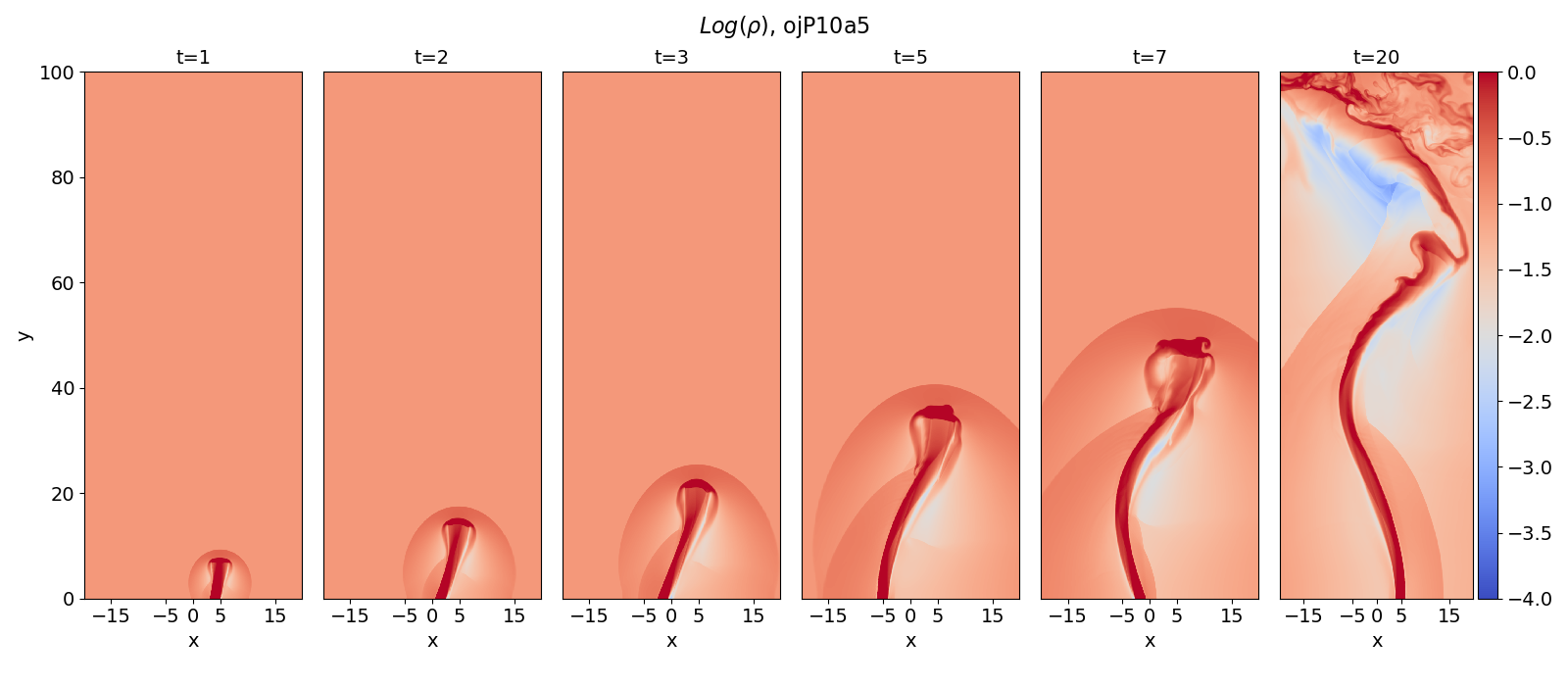
Figure 1: Jet propagation from an orbiting jet source for run ojP10a5. Shown is the density evolution for times $t=1,2,3,5,7,20$.

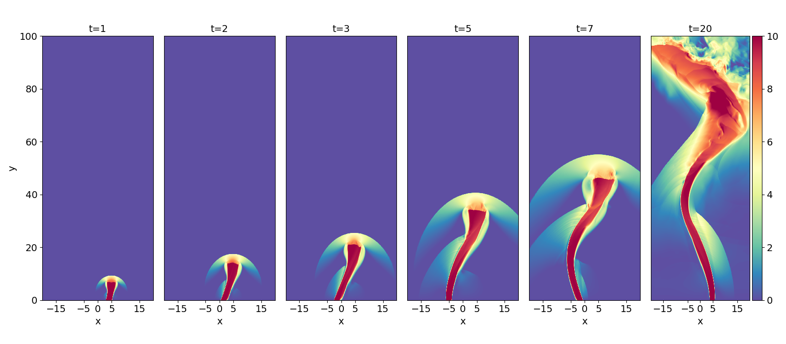
Figure 2: Jet propagation from an orbiting jet source for run ojP10a5. Shown is the vertical speed for times $t=1,2,3,5,7,20$.

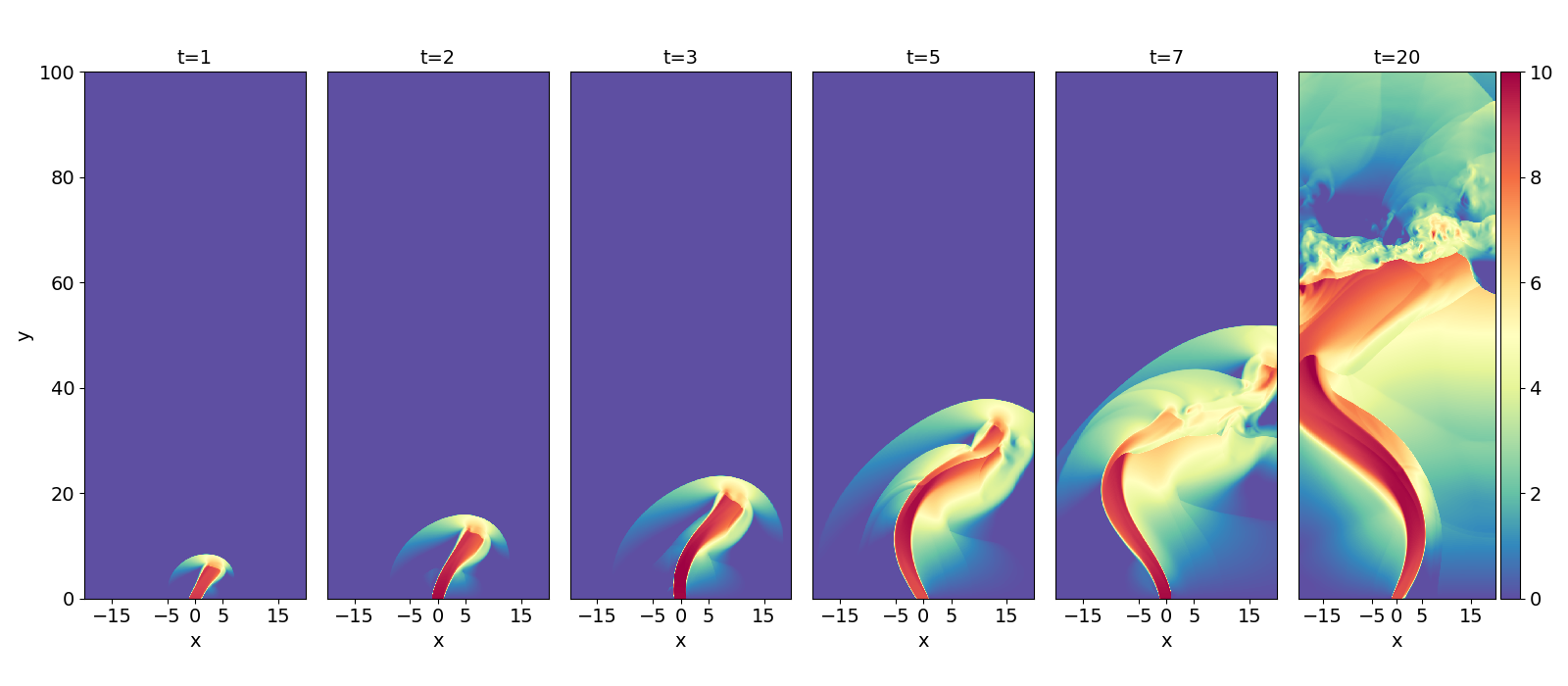
Figure 3: Jet propagation from a precessing jet source for run pj30deg. Shown is the vertical speed for times $t=1,2,3,5,7,20$.

4 Jet nozzles

The definition of the jet nozzle is the fundamental boundary condition in our simulation setup. It defines the injection properties of the jet and, thus, governs the path of the jet and also its interaction with the ambient gas, together with the properties of the ambient medium.

4.1 Spatially fixed nozzles

A spatially fixed jet nozzle is the standard setup that is used in almost all of the literature, starting with seminal papers (see e.g. Stone & Norman 1993a) and is applied also for many recent simulations (Mignone et al., 2005; Banerjee et al., 2007; Keppens et al., 2008; Carroll et al., 2009; Sheikhnezami & Abgharian-Afoushteh, 2019). Spatially fixed nozzles that prescribe a time-variation of the jet injection (density, velocity) lead to pulsed jets (Stone & Norman, 1993b). This setup may provide periodic ejection of jet knots that are similar to observational features. The setup, however, does not explain a mechanism that leads to a time-dependent ejection. Recent approaches were applied to find periodic ejection of knots by a time-dependent disk dynamo mechanism that modifies the mass injection from the disk into the outflow by a variation of the disk magnetic flux (Stepanovs et al., 2014).

Applying multiple jet nozzles that are directed in different directions, colliding jets could be investigated (Cunningham et al., 2006). Also, the case of jets affected by side winds was investigated (Lebedev et al., 2004).

We will not further investigate a spatially fixed nozzle for injection but will apply jet nozzles that move in space.

4.2 An orbiting nozzle

The model setup of an orbiting jet source is interesting for a number of astronomical sources. Stars can be born as binaries and to investigate a binary setup for a protostellar yet is therefore interesting (see Fendt & Zinnecker 1998 for an extensive discussion). Jet launching conditions such as a strong magnetic field and an accretion disk can be present also in cataclysmic variables and high mass (compact star) binaries, and the question arises why not so many of these systems have jets. There is also strong indication that some extragalactic jets may also be launched from supermassive black hole binary systems (Begelman et al., 1980; Roland et al., 2013; Woo et al., 2014; Kharb et al., 2017; Jaiswal et al., 2019). If the jet is launched from one of the black hole system, its orbital motion may play a role.

With our model setup for an orbiting jet nozzle, we want to investigate how the motion of the orbiting jet source does affect the jet propagation on larger scales, and whether these effects can possibly be observed. We also want to investigate whether there exist critical system parameters that prohibit large scale jet motion.

For our numerical setup in 2D Cartesian coordinates we approximate the orbital motion of the jet source as follows. The jet nozzle with radius $\Delta x\equiv 1$ is located at $x_{\rm nzz}(t)$. The motion of the jet nozzle is described by a sin function, $x_{\rm nzz}(t)=a\cos(\Omega t)$, where $a$ is the binary separation, and $\Omega$ is defined by the orbital period $P_{\rm o}=2\pi/\Omega_{\rm o}$. Material of density $\rho_{\rm jet}$ is injected with speed $v_{\rm jet}$ from all ghost cells a position $x$ with $x_{\rm nzz}(t)-\Delta x<x<x_{\rm nzz}(t)+\Delta x$.

In code units $\Delta x=1$. Thus, the choice of the jet radius also determines the length scale of the system. The dynamical timescale is computed from $t_{\rm dyn}=1/v_{\rm jet}$. This becomes essential when we re-scale from code units to astrophysical units.

Obviously, the strength of the effects that we want to compute depends directly on the choice of the parameters $a$, $P_{\rm o}$, and $v_{\rm jet}$. In our simulations, we have applied a parameter choice that demonstrates these effects most clearly. We may relate these simulation parameters to astrophysical units, even to different astrophysical sources, however, it is clear that a perfect match which nature cannot be reached.

In order to demonstrate the physical processes most clearly, we choose $a=5\Delta x$. As said, a suitable scaling of these code units depends on the astrophysics of the jet source. For young stars, the following scaling seems plausible, $\Delta x=10$ au, thus $a=50$ au for our simulation model.

The timescale in code units is thus $t_{\rm dyn}=0.1$ for a jet speed of $v_{\rm jet}=10$. For the orbiting jet sources, the orbital period chosen is $P=10$ corresponding to 100 dynamical timescales. The astrophysical timescale of jet propagation for this choice is $t_{\rm dyn}=10\,\rm au/50\,\rm km/s=0.94\,\rm yrs$ for a jet speed of $v_{\rm jet}=50\rm km/s$, or

$$t_{\rm dyn}=1.6{\rm yrs}\left(\frac{R_{\rm jet}}{10\,\rm au}\right)\left(\frac{v_{\rm jet}}{30\,{\rm km/s}}\right)^{-1},$$ (6)

which could then be connected to the orbital period $P=100t_{\rm dyn}=160$ yrs. From this we calculate a total stellar mass of

$$M_{\star}=4.7M_{\odot}\left(\frac{a}{50\rm au}\right)^{3}\left(\frac{P_{o}}{160\,\rm yr}\right)^{-2}.$$ (7)

Note that $M_{\star}\propto R_{\rm jet}v_{\rm jet}^{2}$, considering the numerical scaling relations applied.

Considering symbiotic stars, there is common agreement that the compact star is a white dwarf below the Chandrasekhar limit. The stellar separations can fall within a wide range, from a few $\rm au$ to $\approx 10~{}\rm au$. The geometrical size of these systems is definitely smaller than for a protostellar binary. Here, for our astrophysical scaling considering the same set of normalized simulation parameters, we find for $a=5\Delta x$ and $a\approx 4\rm au$ a jet radius of $\Delta x=0.8~{}\rm au$.

Thus, the dynamical timescale (again in code units $t_{\rm dyn}=0.1$) would be

$$t_{\rm dyn}=14{\rm days}\left(\frac{R_{\rm jet}}{0.8\,\rm au}\right)\left(\frac{v_{\rm jet}}{100\,{\rm km/s}}\right)^{-1}$$ (8)

Assuming again an orbiting period of $P=100$, corresponding to 3.8 yrs, the total stellar mass would be

$$M_{\star}=4.4\,M_{\odot}\left(\frac{a}{4\,\rm au}\right)^{3}\left(\frac{P_{o}}{3.8\,\rm yrs}\right)^{-2},$$ (9)

which is consistent with our assumption for symbiotic stars.

We emphasize that we do not intend to fit certain systems. The previous estimates do only intend to show that our simulations results can be brought in rough agreement with the different sources. In particular, the jet speed applied is underestimated, which in turn emphasizes the effects of the lateral motion we want to demonstrate.

We note that in our simulations, $v_{\rm jet}$ is typically quite larger than the prospective orbital speed of the jet source. We may therefore neglect this orbital speed and the corresponding centrifugal forces, in agreement with our setup of neglecting gravity for our simulations (see, however, Masciadri & Raga 2002 who performed 3D simulations).

The results for the initial jet evolution are shown in Fig. 1 for the density and in Fig. 2 for the vertical velocity. We clearly see a periodic jet bending.

The curvature and wavelength of the jet bending depend on the orbital period, the jet speed and the the stellar separation. For the parameters applied, we find the amplitude for the curved jet motion being initially similar to the orbital radius. This may be somewhat expected. For the second jet "wave" the amplitude increases to about two orbital radii. The wavelength of the curved jet propagation is about ten orbital radii.

For a bipolar jet source, the evolving flow structure is mirror symmetric with respect to the mid-plane, respectively the orbital plane. Thus, a jet emitted from an orbiting jet nozzle shows a C-shaped structure on larger scales. However, with time also the conditions with in the jet channel and the environment change, and the question arises how long such a periodic structure will survive on the long term. We will investigate this question in Sect. 7.

4.3 A "precessing" nozzle

Indication for jet precession has been observed in a number of sources of different classes. Precession is expected for jet sources in binary systems in cases that the rotational and orbital axes are misaligned.

Since precession is most probably a result of the binarity of the jet source, we would expect effects due to the orbital motion as well for the precessing nozzles. However, for the sake of simplicity we do not investigate the combined action of binary effects here and prefer to disentangle the effects caused by either orbital motion or jet precession. We also note that the precession timescale is usually many orbital timescales. We thus expect the two effects to work on different time scales and can treat them separately. In principle, our setup would allow us to put a precessing nozzle on an orbit and measure the combined effect – prescribing a similar time scale, $P_{\rm orb}\simeq P_{\rm prc}$. However, we expect that from the results of simulating the combined effects, it would be almost impossible to disentangle the origin of certain features.

The precession period ($P_{\rm prec}$) can be related to the orbital parameters as

$$P_{\rm prec}=\frac{64}{15}\pi\frac{M_{\rm p}}{M_{\rm s}}\left(\frac{a}{R}\right)^{3}\sqrt{\frac{R^{3}}{GM_{\rm p}}}\frac{(1-e^{2})^{3/2}}{\cos i}$$ (10)

(see e.g. Beltrán et al. 2016), that can also be applied to wide binaries (Papaloizou & Terquem, 1995). Here, $M_{\rm p}$ and $M_{\rm s}$ are the mass of primary and secondary stars respectively, $R$ is the radius of the disk, $a$ is a separation between binary stars, $e$ is the eccentricity of the orbit, and $i$ is the inclination of the binary orbit with respect to the plane of the disk.

For close binaries, the spin axes and the orbital plane of the sources are expected to be aligned via the magnetic forces. However, (super)outbursts may cause a certain degree of misalignment. Superhumps, defined by their light curve and are caused by super-outbursts, arise rapidly but fade on time scales longer than the orbital period. Therefore, the relation between the superhump period $P_{\rm sh}$ and the respective orbital period $P_{\rm orb}$ is $P_{\rm prec}=P_{\rm orb}P_{\rm sh}/(P_{\rm sh}-P_{\rm orb})$ (Warner, 1995).

We approximate the precession motion of the jet source in our 2D Cartesian setup as follows. The jet nozzle with radius $\Delta x\equiv 1$ is now located at the radius $x_{\rm jet}(t)=0$. The jet is injected in a prescribed direction $\alpha_{\rm jet}$ (measured from the rotational axis) that varies in time, $\alpha_{\rm jet}(t)=\alpha_{\rm jet,max}\cos(\Omega_{\rm p}t)$, between the angles of maximum deflection, $\alpha_{\rm jet,min}$ and $\alpha_{\rm jet,max}$. $P_{\rm prec}=2\pi/\Omega_{\rm p}$ and we consider $P_{\rm prec}=10$ in code units for all precessing nozzle simulations.

The jet speed $v_{\rm jet}$ remains constant in time, however the velocity components of the injected jet vary over time as the direction of the nozzle changes, $v_{x,\rm jet}=v_{\rm jet}\sin(\alpha_{\rm jet})$, and $v_{y,\rm jet}=v_{\rm jet}\cos(\alpha_{\rm jet})$.

In Figure 3 we show the initial time evolution of the system, applying $P_{\rm p}=2\pi/\Omega_{\rm p}=10$, $v_{\rm jet}=10$, and $\alpha_{\rm jet,max}=30\arcdeg$. The same time scaling as it is described for the orbiting jet source applies, thus $t_{\rm dyn}=1/v_{\rm jet}$.

We immediately see the essential difference to the model of an orbiting jet source, such that for a bipolar jet, the evolving flow structure is mirror symmetric with respect to the origin. Thus, a jet emitted from a precessing nozzle shows a S-shaped structure on larger scales.

Figure 4: Hydrodynamic jet evolution for different orbital parameters, shown at time $t=70$, for combinations (from left to right) of periods and separations $(P=10,a=5)$, $(P=25,a=5)$ and $(P=25,a=10)$, corresponding to simulation runs ojP10a5, ojP25a5 and ojP25a10, respectively.

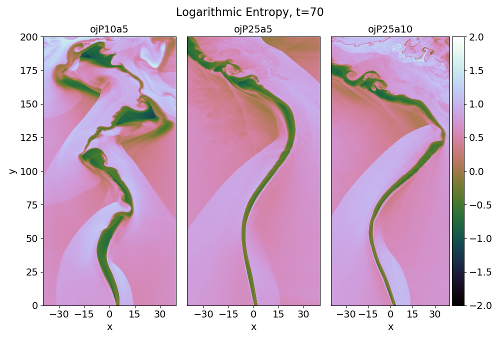
Figure 5: Same as Fig. 4, but for the measure of entropy $K\equiv P/\rho^{\gamma}$ (in log scale).

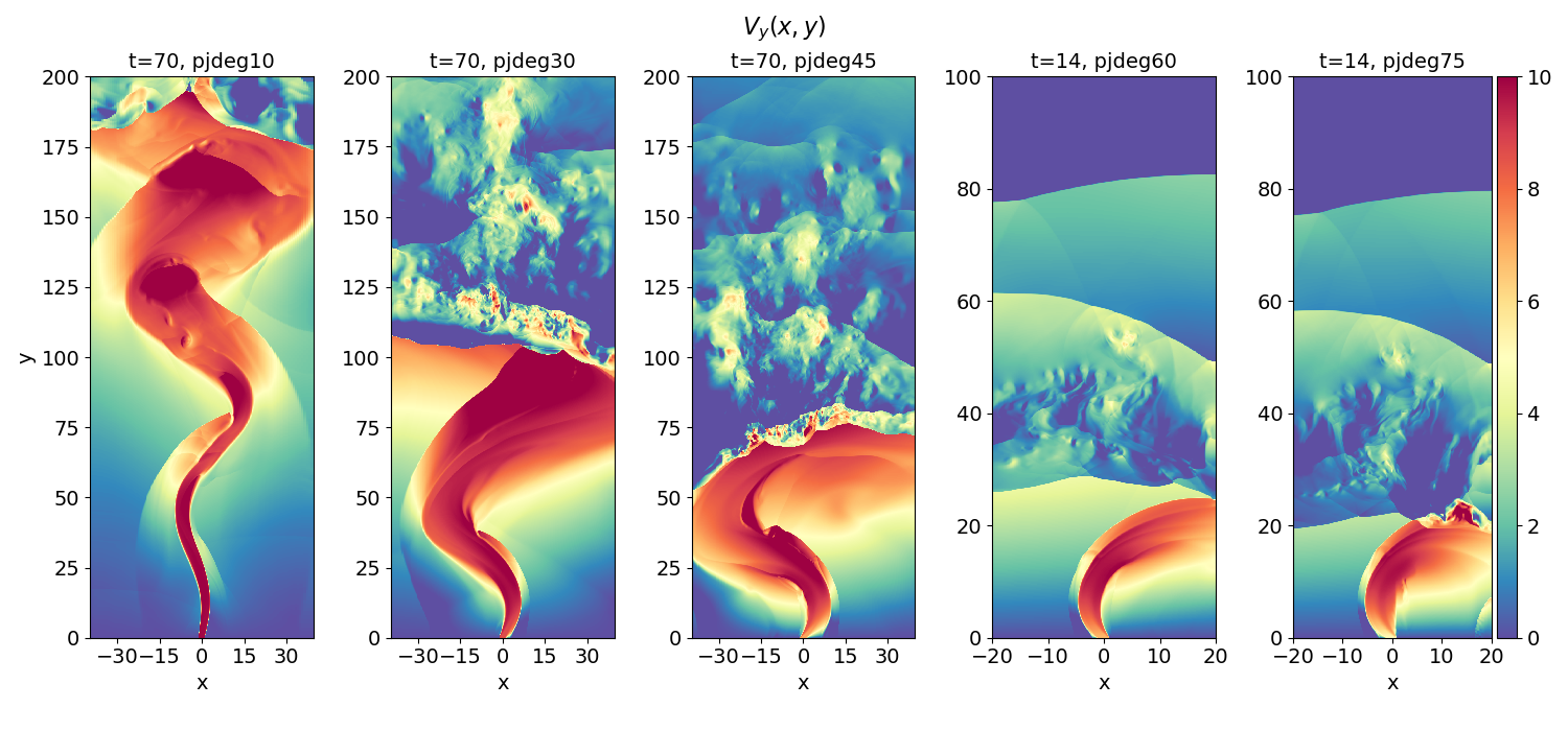
Figure 6: Hydrodynamic evolution for jets of different precession angles, $\alpha=10,30,45,60,75^{\circ}$ (from left to right), corresponding to simulation runs pjdeg10, pjdeg30, pjdeg45, pjdeg60 and pjdeg75, at time steps $t=70,70,70,14,14$, respectively. Note that a large injection angle $\alpha>45^{\circ}$ for the nozzle results in a jet propagation that fails to reach large distance.

5 C-shaped jets from orbiting jet sources

We now discuss our simulation results on intermediate time scales for the setup of an orbiting jet nozzle (see Sect. 4.2). Figure 4 shows the evolution of the jet beam at the same time for different orbital parameters, but at the same evolutionary time step $t=70$. All simulations were initiated with the same initial conditions for the ambient medium, $\rho_{\rm ism}$, $P_{\rm ism}$, and run with the same injection parameters for the jet $\rho_{J}$, $P_{J}$, $v_{J}$. However, different orbital periods and orbital separations were applied. Naturally, we would expect a correspondence between the jet stability on larger scales with these parameters that determine the "disturbance" of a straight jet motion.

The disturbed jet propagation is characterized by its curvature, that is, a combination of the wavelength and the amplitude of the perturbed jet geometry. Obviously, the jet curvature is determined by the orbital separation (defining the amplitude), and the time scales for the orbital motion and the jet speed.

For the examples shown, we find that the wavelength $\lambda$ of the jet propagation seems to be determined by the orbital period rather than by the orbital separation (about $\lambda\simeq 40$ for $P=10$, and $\lambda\simeq=60$ for $P=25$). On the other hand, the amplitude $A$ of the jet bend seems determined by the orbital separation (about $A\simeq 10$ for $a=5$, and $A\simeq 15$ for $a=10$).

Another signature that can be easily derived from the simulation result (and can be compared to observed sources) is the length of the jet. We clearly see that the simulations considering a wide orbital radius $a=10$, become unstable the earliest. In particular, these jets injected do not survive long and do hardly reach the upper boundary. Typically, the jet flow is smooth and well defined for at least one bend, after which some of the flows break up, depending on the orbital parameters.

From the astrophysical point of view, these jets are shorter and do not penetrate the ambient medium for long. The jet energy is converted into thermal energy more efficiently due to the large effective surface of the jet. Note that the kinetic energy flux of all these jets is the same.

We also find a clear relation between the wavelength and the amplitude of the jet bending and the orbital parameters. The shorter the orbital period (for the same stellar separation) the shorter the wavelength. Altogether, these seem to be too strongly disturbed and do not survive long when propagating. Astrophysically, such systems correspond to binaries containing a relatively massive primary (the jet being ejected from the secondary), for example a massive compact primary with a low mass stellar companion. Here, we do not consider here gravitational torques (see for example Sheikhnezami & Fendt 2015, 2022), but alone from the orbital motion of the jet source, we may conclude that such binaries may not eject stable narrow jet streams propagating much longer than the respective orbital separation. This is in nice agreement with long-term 3D simulations of MHD jet launching in binary systems which find a critical inclination between accretion disk and orbital plane of about $10-20\arcdeg$, resulting in a precession cone of the jet of $8\arcdeg$ (Sheikhnezami & Fendt, 2018).

Jets originating from binaries with small separation and short orbital period, however, are able to travel as turbulent beams to relatively long distances. We understand that this becomes possible, as due to the small orbital separation the jet injections over time widen the funnel that was already drilled by the previous injections, resulting in a clean and broad jet funnel. In contrast, for jets originating from binaries with wider separation, each jet injection (over time) practically bores its own funnel into the ambient medium. Thus, instead of a single wide funnel the jet injection produces its own small funnel. These small funnels are, however, terminated when the jet injection continues on its orbit, and ejects in new directions.

In Fig. 5 we show the entropy maps for simulation runs ojP10a5, ojP25a5, and ojP25a10. Entropy can show the origin of the gas as it labels the gas temperature, thus showing whether we see cool (dense) gas that was injected by the jet nozzle, or hot gas (of the originally low density gas of the ambient medium).

We see that at the turning points of the jet motion the matter is pushed further, and a shock front is formed. Here, the kinetic energy is transferred to the shocked gas, heating it (to larger entropy). The backside of the shock stays cool. Across the shock front, the entropy increases, especially in the turning points of the jet mentioned above, while the inner jet stream has low entropy. Whenever a shock is produced, it disrupts the continuity of the flow, causing a turbulent flow pattern. However, at these turning points, the flow accumulates into filament-like structures. These structures depend somewhat on the shock properties. The first panel of Fig. 5 clearly demonstrates the generation of turbulence across the turning points of the jet.

We finally note that these are 2D simulations and that the bent or disturbed jet structure will certainly give rise to further jet instabilities, such as kink modes or shear instabilities.

The amplitude of the jet bending seems simply related to the orbital separation. The larger the orbital separation the larger the amplitude. However, for the same amplitude, the wavelength becomes larger for larger orbital periods.

A well-known example for a C-shaped jet structure is HH 211, for which binary components of different mass are discussed that may cause the jet bending (Lee et al., 2009). Another C-shaped jet source is HH 212 (see e.g. Lee et al. 2015; Noriega-Crespo et al. 2020), again the deviation from the linear motion is discussed in terms of a binary motion of the jet-ejection star.

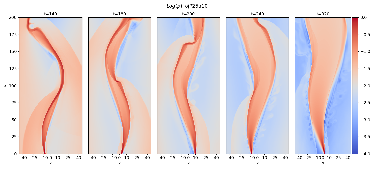
Figure 7: Long term evolution for run ojP25a10. Shown is the density in log scale for time steps $t=140$, $t=180$, $t=200$, $t=240$, and $t=320$.

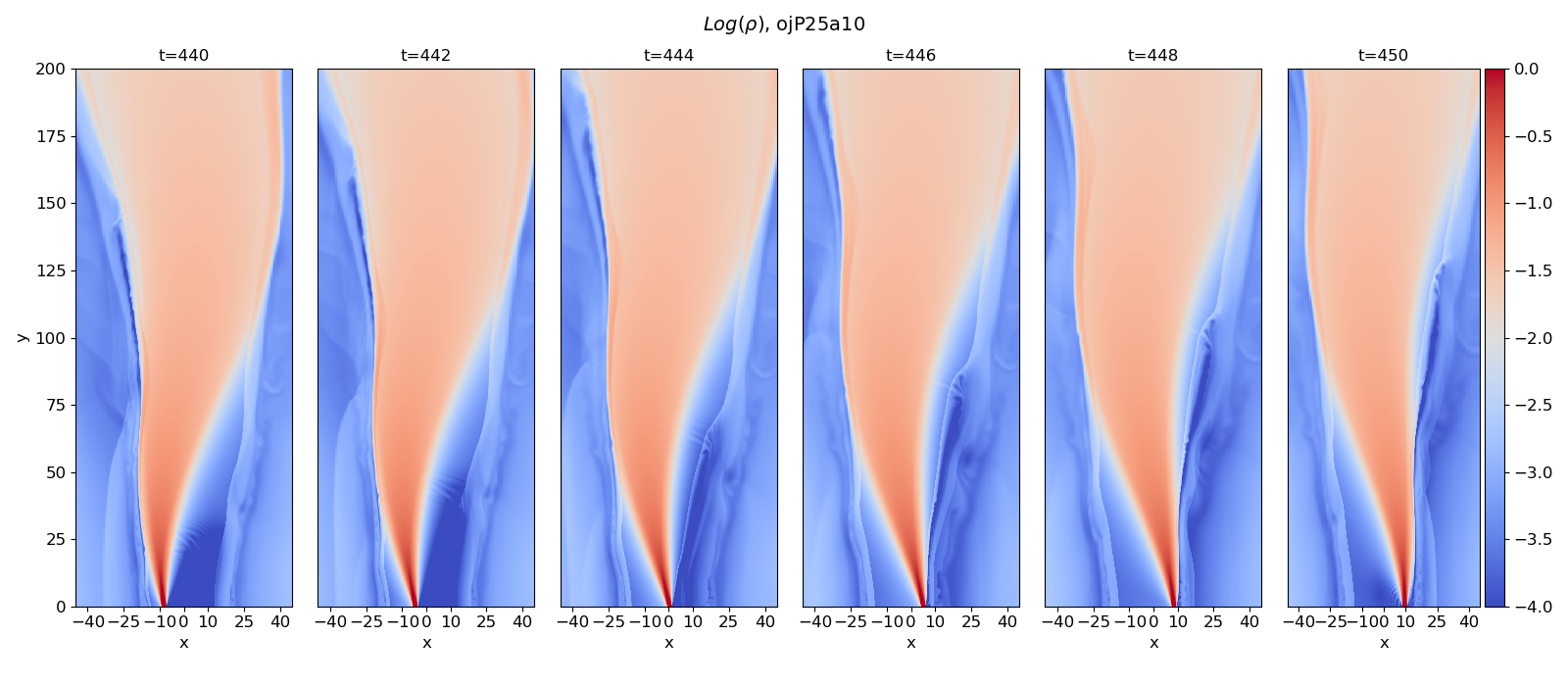
Figure 8: Late-time evolution for simulation ojP25a10 from $t=440$ to $t=450$. Shown is the density in log scale for a sequence with high time resolution, $\Delta t=2$.

6 S-shaped jets from precessing jet sources

We now discuss our simulation results on intermediate time scales for the setup of a precessing jet nozzle (see Sect. 4.3). Figure 6 show the evolution of the jet beam at the same time for different precession angles of the jet nozzle at time $t=70$ for the longitudinal velocity distribution.

We clearly see how the opening angle of the precession cone affects the jet propagation on longer scales. Jet beams that are ejected along a widely opened cone, do not propagate very far. The critical angle is between $10\arcdeg$ and $20\arcdeg$, but of course, also depends on the further jet kinematics. We explain this as follows. For large precession angles the momentum that is injected into the jet in the direction of the axis of the precession cone, is not sufficient for penetrating the ambient medium. The latter is stirred up, as visible in the turbulent-looking structure and the shock(lets) that are moving away from the jet-ISM interface.

These outflows may for example trigger a local collapse in the ISM. However, their penetration depth is some 50-100 initial jet radii only. The outflow moves along their outflow cone with almost their injection speed, but are quickly halted at the shock that develops at the very front of the outflow.

For precession angles $<45\arcdeg$, at early times, the jet flow shows a C-shape geometry. As time progresses, the jet stream begins to turn into an S-shaped form. For larger precession angles an S-shaped jet could not be produced. As it does not propagate sufficiently long distance due only a short-reaching C-shaped jet appears, see Fig. 6.

Another interesting feature we note is the jet curvature increases with distance from the injection. For example, simulation pjdeg10 that applies a nozzle opening cone of only $2\times 10\arcdeg$ evolves into much more curved structure before the jet terminates. In fact, with each wiggle (there are three of them), the curvature radius decreases, from say 30 to 15 to 10. In fact, the reason for the jet termination is exactly this decrease of the corkscrew pitch angle, that leads to a constant momentum loss along the original jet direction. In the end, the jet has lost too much of its momentum and cannot easily penetrate further.

When the jet curvature increases, material accumulates at the turning points of the jet.

Along the jet stream, the jet opening cone expands on large distances. We see an indication that jet knots are produced (in particular for simulation pjdeg10).

On the other hand, the wiggling of the highly inclined jet ’tail’ introduces shock waves into the ambient gas, best seen for pjdeg60 and pjdeg75 simulation runs seen in the velocity slices in Figure 6 (right). The shock separation and shock speed are determined mostly by the precession time scale. The shocked material is moving with a speed $v_{\rm s}\simeq 2$, defining a timescale between the shocks of $\Delta t_{\rm s}=\Delta y/v_{\rm s}\simeq 30/2=15$. This timescale is in good agreement with the precession timescale $P_{\rm prec}=10$.

Even when the jet propagation is limited in distance, more and more material is injected into the jet channel. As it cannot propagate further, this material is accumulated and the jet head broadens.

Many protostellar jets are observed only one-sided, but there are prominent examples that show a S-shaped propagation patter, such as L1157 (Podio et al., 2016). Another example is MHO 2147 (Ferrero et al., 2022) that also seems to follow the analytical trajectories for precessing jets proposed by Masciadri & Raga (2002). A further protostellar jet indicating on precession is DO Tau (Erkal et al., 2021).

For the symbiotic system R Aqr jet components can be traced to up to $\sim 900$ au, which is quite long compared to the binary separation of $\sim 15$ AU. The jet is surrounded by an outflow of a wide opening angle filled with low excitation gas. Melnikov et al. (2018) mention the origin of the gas emission can be cold stellar wind, especially from mass losing Mira variable and partly collimated jet. This observational findings could be nicely matched by our simulations such that this cocoon is filled by shock gas at the locations when the wave of the jet stream has its turning points. This wide opening cone along the jet we see in particular in our long time step simulations. Melnikov et al. (2018) in particular mention the S-shaped jet in the inner part of the wide-outflow close to the stellar system which is exactly what we find in our long-term simulations (see below).

Another example of a curved jet is CH Cyg (Karovska et al., 2010), another symbiotic star. Interestingly, this jet is changing its morphology over time between S-shaped and C-shaped. Its shock front is propagating with <100km/s and is slowing down since 2001. The authors suggest that this jet can be produced by an episodically powered precessing jet or continuous precessing jet with occasional mass ejections or pulses due to the structure of the jet. CH Cyg may thus be a good example of a jet where both the nozzle effects discussed above can play a similar role, and the jet structure that is visible is originally triggered by a time-variable feeding to the jet. It would be thus interesting for a future simulation to simulate a precessing and orbiting nozzle in order to find transitions in morphology.

We note that at this stage we cannot intend to fit certain courses as many important dynamical parameter are observationally not yet determined. We are left with finding similarities in the jet propagation that may hint on the nature of the jet source, such as precession vs. orbital effects.

7 Long-term evolution: transition to a wide jet channel

We now investigate how the jet propagation evolves on much longer time scales. We have seen above that for intermediate time scales (and for particular system parameters) the jet evolves as a bent, wavy structure, similar to a rope that is perturbed at one end. The wave pattern propagates until it terminates at the bow shock.

This picture changes when we consider much longer time scales. In Figure 7 we show the evolution of the same injection model that we considered above (see Fig. 1), but for times $t=140$ to $t=320$. We find that the wave pattern broadens such that the wavy channel of the jet flow becomes wider and wider. However, the jet flow is still oscillating.

At some point in time, the lateral motion of the oscillating jet has produced a conical-shaped outflow channel with a geometry that has become rather steady in time. This happens roughly for times $t>400$ (see Fig. 8). The half opening angle of the cone is about 15°.

The width of the cone at the injection point is about the orbital diameter. The jet nozzle orbits within this cone, while the injected jet material is distributed over the whole width of the conical outflow. This can be seen in Fig. 8 where we show the evolution in high time resolution. The wave pattern of the jet motion is gone. However, the boundaries between the wide jet flow and the ambient gas are not straight, but still show a kind of wavy structure, but this seems to be decoupled from the forcing perturbing the jet injection. The orbital jet nozzle still governs the initial jet flow and imprints a periodic wiggling on it. However, on more distant scales the lateral outflow seems decoupled from the motion of the nozzle.

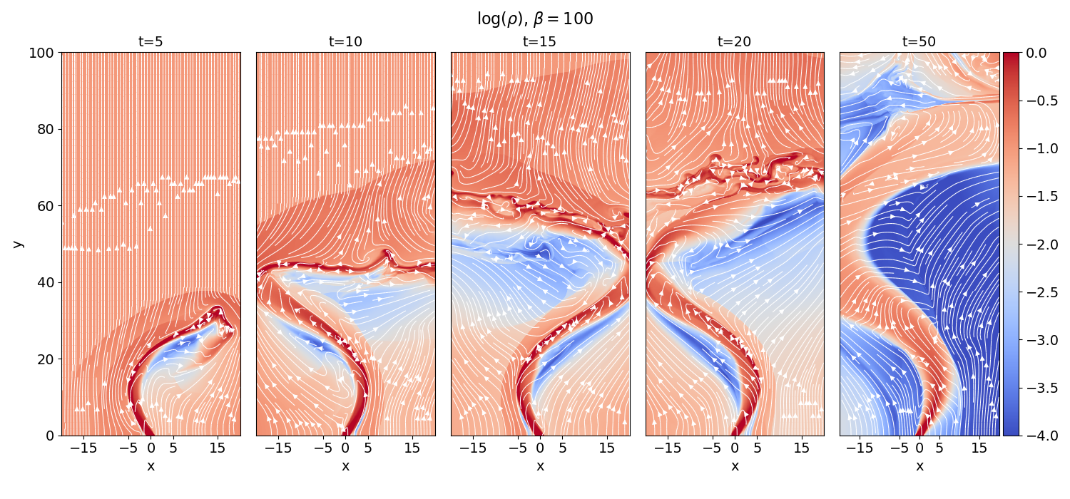
Figure 9: Time evolution of the magnetized simulation pj30degB100 with a maximum precession angle of $\alpha_{\rm max}=30\arcdeg$ and for $\beta=100$. Shown is the density distribution (colors) and the magnetic field lines (white) for the time steps $t=5,10,15,20,50$ (left to right).

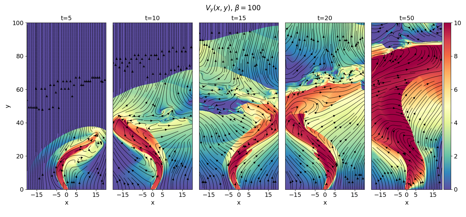
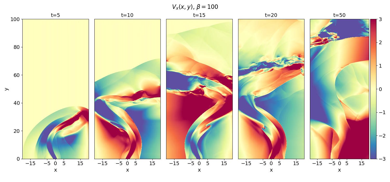
Figure 10: Time evolution of the magnetized simulation pj30degB100 with a maximum precession angle of $\alpha_{\rm max}=30\arcdeg$ and for $\beta=100$. Shown is the vertical (top) and horizontal (bottom) velocity distribution (colors) and the magnetic field lines (black) for the time steps $t=5,10,15,20,50$ (left to right).

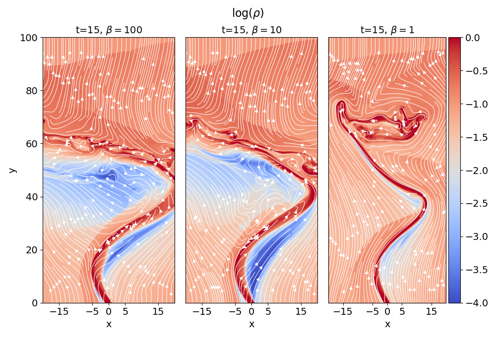
Figure 11: Precessing jets injected into an ambient gas of different plasma beta. Shown is the density and magnetic field lines at time $t=15$ for $\beta=100,10,1$ from left to right, respectively. The precessing angle of the jet nozzle is $\alpha_{\rm max}=30\arcdeg$.

8 Impact of the magnetic field

Astrophysical jets are magnetized. We know that jet launching is in general a magnetic phenomenon requiring a large-scale magnetic flux in the jet driving source (Blandford & Znajek, 1977; Blandford & Payne, 1982; Casse & Keppens, 2002; Hawley et al., 2015). Also, the medium into which the jet is injected is magnetized.

An interesting question is the alignment of protostellar jets with the magnetic field in the ISM. This still seems to be an open issue with various papers providing different answers (Targon et al., 2011; Hull et al., 2013; Pudritz & Ray, 2019; Hirano & Machida, 2019). In our treatment, for simplicity, we adopt a magnetic field geometry that is aligned with the average jet injection axis. This allows disentangling the magnetic effects most clearly.

8.1 The question of a toroidal field

It is clear that magnetized jet typically carries also a toroidal magnetic field. This comes as a natural consequence of MHD models, as the inertia of the jet material induces a toroidal field from the poloidal component (Blandford & Payne, 1982; Uchida & Shibata, 1985; Stepanovs & Fendt, 2016). The toroidal field plays an important role for jet collimation and stability, however, it is likely impossible to implement it in a 2D Cartesian setup in a consistent way.

A possible approach may be to inject a $B_{z}$ component that is anti-aligned left and right from the jet axis. However, this approach is yet untested in the literature and its benefit is maybe little. Jet collimation and stability are not of interest to the present study. What we neglect here, is thus mainly the magnetic pressure by the 3rd field component. Tension forces by the 3rd field component cannot be derived are as its curvature cannot be considered in a 2D slab approach. Overall, the main effect of the 3rd field component would be an enhanced overall jet pressure, which could, however, mimicked by applying an increased gas pressure.

We note that without considering a toroidal magnetic field (thus neglecting poloidal electric currents), we cannot investigate possible jet bending by Lorentz forces, $\vec{F}_{\rm jet}\propto\vec{j}_{\rm jet}\times\vec{B}_{\rm ism}$, as previously suggested by Mundt et al. (1990) or Fendt & Zinnecker (1998).

8.2 A magnetized precessing nozzle

We have re-run the hydrodynamic simulations with a different ambient poloidal field strength, defined by the plasma beta $\beta\equiv P/B^{2}$, where $P$ is the initial gas pressure (of jet and ambient gas) and $B$ is the strength of a constant magnetic field in vertical direction (aligned with the mean direction of injection).

For this section, we have concentrated our discussion on the model setup of a precessing jet nozzle. We have found that the main effects of the magnetic field on the curved jet motion in the simulations for an orbiting nozzle are basically the same (see below and the Appendix).

Assuming a constant magnetic field implies that the initial field is in fact force-free with no magnetic pressure or magnetic tension forces imposed. Any material motion perpendicular to the field direction will induce perpendicular field components which then lead to Lorentz forces providing feedback to the original jet propagation.

Figure 9 shows the time evolution of density and magnetic field for simulation pj30degB100. Here, a maximum precession angle of $\alpha_{\rm max}=30\arcdeg$ and a plasma-beta of $\beta=100$ is applied. We clearly see the magnetic field is perturbed by the jet motion. The dynamics of the wiggling jet is dominating the field distribution. The field lines tend to follow the jet motion with exposing a similar curvature.

Similar behavior can be seen in the velocity distribution in Figure 10. Notably, the velocity distribution is substantially broader than the density distribution. The reason is the material that has been entrained along the high-speed jet. Obviously, this holds for both the vertical and horizontal velocity components.

In Figure 11 we compare examples of our simulations. Here, a vertical field of different strengths was supplied to the pure hydro setup of simulation pj30deg. The injection nozzle was assumed to precess with an opening cone of $30\arcdeg$. The plasma beta imposed initially is $\beta=100,10,1$.

The simulations clearly demonstrate the stabilizing effect of the magnetic field. While for high plasma beta the wiggling jet dominates the magnetic field and thus wiggles the magnetic field along with the time-dependent jet injection, this wiggling of the jet (also compare to the hydro case) and the magnetic field is weaker for a low plasma beta. As a consequence, the jet motion remains relatively undisturbed, and the stream can reach further distances from its injection site.

This can as well be seen in Figure 12 and Figure 13, now applying a stronger magnetic field. In particular for the simulation with $\beta=1$ (pj30degB1), the evolution of the jet follows a rather straight trajectory, despite the same precession angle of the nozzle. While the jet propagation follows initially (in time and space) a rather curved trajectory that is triggered by the injection nozzle, on longer spatial scales the jet propagation will straighten, and will finally reach substantial longer distances compared to lower field strength.

For very long simulation times ($t>200$, not shown), we see an interesting change in jet geometry such that the jet amplitude widens again as the ambient gas becomes diluted and with it the ambient pressure that confines the jet. For an intermediate field strength applying $\beta=10$ (pj30degB1) the field is not sufficiently strong in order to collimate the wiggling jet flow such that if follows a narrow channel and can reach large distance.

8.3 The force balance across the jet

In order to understand the motions in the system of jet and ambient medium, we can look at the force balance across the jet distribution across the system. As the pressures do not remain constant during the evolution, forces arise that affect the jet propagation and the distribution of the ambient gas.

In Figure 14 we show the profiles for the different force contributions. Here, we consider simulation pj30degB100 with a high plasma-beta $\beta=100$, at time $t=20$ and for different layers across the jet, $y=20,30,40$ (see also Figure 9 for a comparison). We display the pressure gradient $\partial_{x}P$, the magnetic pressure gradient $\partial_{x}(B^{2}/2)$, and the magnetic tension $\vec{B}\cdot\nabla)\vec{B}$ which in x-direction is $B_{x}\partial_{x}B_{x}+B_{y}\partial_{y}B_{x}$.

The profile drawn across the jet at altitude $y=40$ (top panel) shows the localized jet disturbance that is embedded in a force-free ambient magnetized gas that is basically unchanged from the initial state. In higher resolution of the jet cross-section, again at $y=40$ (2nd top panel), we see that the force components in the jet almost balance, indicated by the dashed pink line. However, just outside the jet (right side) the negative pressure rises again and remains unbalanced, giving rise to a force to the ’left’ direction, thus pushing the jet to the left.

Going down along the jet to $y=30$ we see similar force profiles with the typical sinusoidal structure. Compared to the $y=40$ slice, here an unbalanced (and positive) force on the left side of the jet appears, resulting again from gas pressure and pushing the jet to the right.

This is similar to a slice at $y=20$, however, here the gas pressure force is relatively larger. We suggest that these high pressure forces arise since we are close to the jet injection nozzle where the jet is injected into the domain, in different directions over time, causing an over pressure. On the contrary, in the upper areas, an under-dense area is established behind the jet when the jet is moving left or right. The negative pressure force decelerates the lateral jet motion.

In all example slices, the area of gas pressure force is similar to the jet area. In general, the magnetic tension force is relatively small compared to the magnetic pressure force. While gas pressure gradients close to the jet affect the lateral jet motion, magnetic pressure force and gas pressure force almost balance within the jet (while changing sign).

Figure 15 shows profiles of characteristic MHD variables from the jet interaction. In particular, it demonstrates how different a strongly magnetized jet behaves. While the entropy measure ($K=P/\rho^{\gamma}$) is similar for the hydro case and the case of low magnetization, the highly magnetized jet ($\beta=1$) is heated much higher temperatures. Note that the hydrodynamics of the jet injection is the same for all models, only a force-free vertical field is added for the magnetic case.

This additional magnetic energy serves as another energy source for jet heating, as the $\beta=1$ jet carries an additional magnetic energy reservoir that is 100 times larger than for the $\beta=100$ jet. On the other hand, the Alfvén Mach number of the strongly magnetized jet is much lower compared to the weakly magnetized jet (while the Alfvén speed is much higher). This, of course, would have consequences for the stability of jet propagation, which we, in our 2D approach, cannot determine.

8.4 Notes on a magnetized orbiting nozzle

As mentioned above, we have concentrated our discussion on models considering a precessing jet nozzle. The main effects of the magnetic field we just described are basically the same for an orbiting nozzle, that is the damping of the jet curvature (see Fig. B.1 in the Appendix).

We close this section, noting that the magnetic field has quite an impact on how the binarity effects influence the jet motion. The (longitudinal) magnetic field damps the lateral jet amplitudes that are enforced by either precession of orbital motion of the jet sources. Concerning jet thermodynamics, the magnetic field seems to serve as an additional energy reservoir that leads to higher temperatures of the has that is shocked at the jet head or at the jet-ambient gas boundary layer.

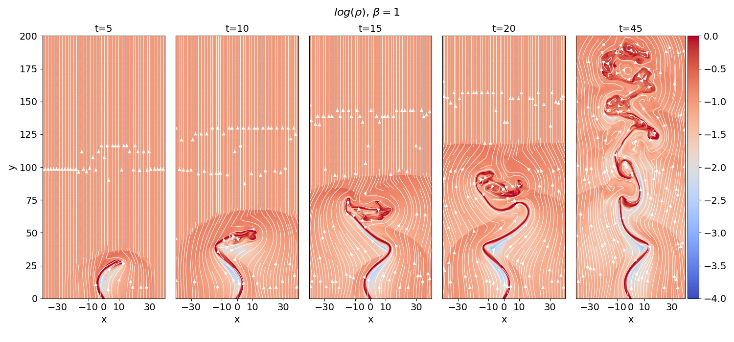
Figure 12: Same as Figure 9 but $\beta=1$, simulation pj30degB1. A larger grid is shown as the jet reaches farther distances.

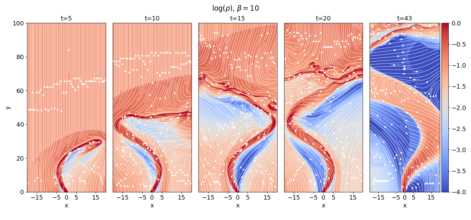
Figure 13: Same as Figure 9 but $\beta=10$, simulation pj30degB10.

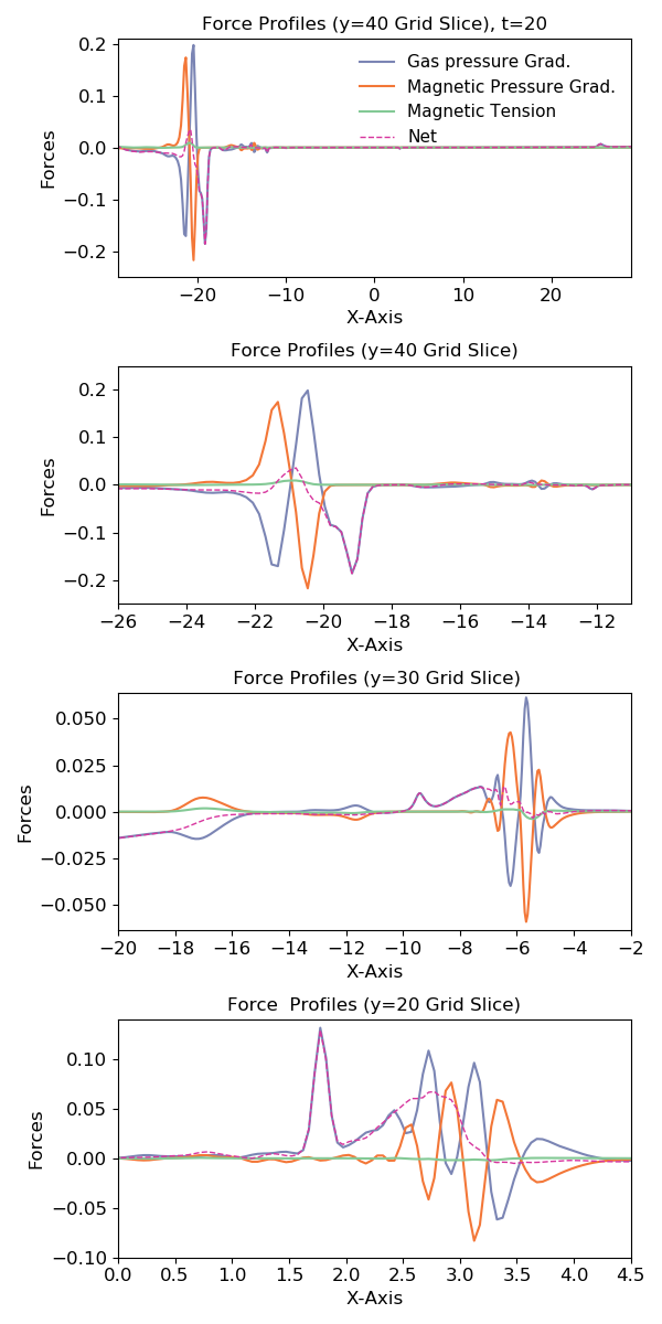
Figure 14: The force profiles with different scales and different y-grid slices for $t=20$ for simulation pj30degB100. The top panel shows forces along the $x$-direction at $y=40$ for the whole x domain, $30\leq x\leq-30$. In the panels below the force profile are shown, zoomed-in to the area around the jet for $y=40,30,20$, respectively. Shown are the gas pressure gradient (blue), the magnetic pressure gradient (orange), the magnetic tension (green), and the net force (dashed pink).

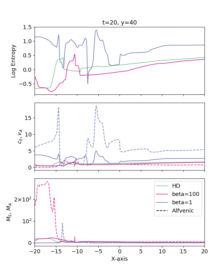
Figure 15: (Magneto-)hydrodynamic key quantities shown as profiles across the jet for simulations pj30deg (hydro, green), pj30degB100 (MHD, $\beta=100$, pink), and pj30degB1 (MHD, $\beta=1$, blue), respectively. From top to bottom, we show the profiles of the measure of entropy $K\equiv P/\rho^{\gamma}$, sound speed $c_{\rm S}$, Alfvén speed $V_{\rm A}$ (dashed), Sonic Mach number $M_{\rm S}$, and Alfvén Mach number $M_{\rm A}$ (dashed).

9 Conclusions

We have applied 2D (M)HD simulations in order to investigate how a precessing or orbiting jet nozzle affects the propagation of a high speed jet. We have performed a parameter study of systems with (i) different precession angle, (ii) different orbital period, (iii) different orbital separation, and (iv) different magnetic field strength.

While a modeling of exact astrophysical parameters is too CP-expensive for our parameter study, our results can be applied for a number of astrophysical systems, such as close or wide binaries, young stars, symbiotic stars, or compact binaries. Our results are as follows.

(i) Both precession jet nozzles and orbiting jet nozzles inject jets that propagate on a curved trajectory. The amplitude and the wavelength of the curved pattern depend on these initial parameters, such as that a wider orbit or a wider opening angle leads to a larger amplitude.

(ii) While jets injected along orbits of large radius produce jets with large amplitudes, the jet motion that is injected by a precessing nozzle is limited by the opening angle of the precession cone. We find a limiting opening angle for the precession cone of about $20\arcdeg$, above with the longitudinal jet motion is too perturbed by precession in order to reach large distances. These jets turn around following a strong side-wise motion and terminate soon in a broad shock region.

(iii) An essential difference between jets from precessing nozzles and orbiting nozzles is that on intermediate length scales, the former show a (bipolar) S-shaped structure, while the latter show a C-shaped structure. Note that due to our 2D approach, this has to be compared to a more realistic 3D structure, projected on the plane of the sky. However, the main features of the S-shape or C-shape will remain, and may be applied to observed sources.

(iv) While on intermediate distances a curved jet structure is revealed, on longer distances, thus also on longer time scales, the persistent jet motion bores a funnel into the ambient medium, wide enough that the jet wave pattern is enclosed. On these length scales, the wave pattern dissolves into a broad stream filling smoothly the conically shaped outflow funnel. The outflow funnel is slightly oscillating, triggered by the time-dependent jet injection geometry.

(v) The consideration of a magnetic field in the ambient medium and the jet (a jet aligned poloidal field) shows the stabilizing effect of magnetic forces (for jets injected by precessing and orbiting nozzles). While simulations with a plasma-$\beta$ of 100 do not differ much from the hydrodynamic case, simulations with $\beta=10$ or even $\beta=1$ produce jets that propagate much further, since the lateral amplitude triggered by the jet injected is damped on intermediate and long distances. The jets remain confined to small jet radii, and the jet lateral amplitude is damped by a factor 2.

(vi) Investigating the force balance across the jet shows the gas pressure and Lorentz force are in good equilibrium in the ambient medium and in the jet - except the region just outside the jet at the concave side. This net force is finally balanced by the dynamical pressure of the lateral motion.

We finally note that our study is limited by the 2D approach. Orbital and precessing jet nozzles do not only move left-right as in our 2D study, but orbit around. The main 3D effect here would be a helical wiggling of the jet stream. However, we firmly believe that their projected geometry and dynamics can be very well approximated by our 2D approach. While studies in the literature have partly addressed these questions, a full, long-term 3D MHD study is still missing, one of the reasons being the huge CPU resources needed. Jet launching simulations in 3D MHD considering binary sources have only recently been published, restricted in size to the Roche lobe and in time to 1-2 orbital periods.

Appendix A Comparison with literature simulations

A number of previous studies have investigated the evolution and propagation of jets that are ejected from orbiting or precession sources (see discussion in Sect.1). In this paper we claim that our 2D Cartesian setup allows to investigate a series of parameter runs which could not be done by previous simulations, in particular for the 3D simulations. It is therefore helpful to provide a table that compares the main simulation characteristics of these simulations with our present setup (see Table 3). One particular difference is that we also investigate the impact of the magnetic field.

In the following, we compare our results of the initial propagation with selected studies from the literature. This is not straightforward as different parameter setups and numerical grids were applied (see Table 3 for a comparison).

For the precessing nozzle, we compare our simulations to the 3D hydro simulations of Cliffe et al. (1996). Both approaches show a wider opening angle of the jet outflow cone for a wider precession cone (see their Fig. 1 and our Fig. 6). Also, when the precession time scale is short, more wiggles are observed (same figures) - interestingly, for a similar precession angle ($12\deg$ vs. $10\deg$) the jet length before termination is similar with about three wavelength. Due to the higher resolution, our simulations show more sub-structure, such as shocked gas in and around the jet. These features may be very relevant for observations. Further, we see a mild widening of the jet beam along its path, while the Cliffe et al. (1996) simulations show a rather constant jet diameter. Both simulations are run with jets in pressure equilibrium with the ambient medium. On the other hand, the overall agreement on the main kinematic structures provides confidence for our 2D slab approach.

The 2D Cartesian simulations of Biro et al. (1995) also show shock structures along the outer sides of the curved jet trajectory. The simulations run for about three precession periods, showing three jet "waves" at this point in time. However, we don’t know how the system will evolve further in time, for example, whether the jet is able to propagate further. The jet stream looks more stable, maybe because it is injected with a substantial over pressure (unlike in Cliffe et al. 1996 or our approach).

We may further compare our results to the 3D simulations of Masciadri & Raga (2002) who investigated orbiting and precessing nozzles in the hydrodynamic limit. Here we find for both simulation setups only one wave pattern along the jet. However, probably due to the high numerical costs, these simulations were evolved only till one orbital or precession period, respectively. Also here, the jet streams stay rather narrow, despite their over-pressure with respect to the ambient gas, and the low jet resolution with $\simeq 3$ cells per jet radius.

Table 3: Comparison of our simulation characteristics with a selection of literature simulations in the. We compare the size of the numerical grid and its geometry, the resolution applied for the jet, the simulation run time, and other specific features of the approach.

Authors	Approach	# grid cells	# cells/jet radius,	Remarks
			run time
Biro et al.	HD, 2D slab	$450\times 450$	10	adaptive grid, incl.
				radiation/chemistry
Cliffe et al.	HD, 3D cart	$128\times 128\times 128$,	5 or 10,
		$256\times 256\times 256$ max	1.5 prec periods
Masciadri & Raga	HD, 3D cart	$64\times 64\times 512$ max	3	adaptive grid,
			3 prec/orb periods	orb. radius $=2.2R_{\rm jet}$
Monceau-Baroux et al.	HD, 3D cart	$72\times 72\times 144$ (base)		Adaptive mesh refinement
		$4608\times 4608\times 9216$ (eff)	68 prec periods
Sheiknezami et al.	MHD, 3D cart	$200\times 200\times 200$	100	launching, no ambient gas,
			1 orbital period	small physical grid
Present study	MHD, 2D slab	$400\times 2000$	20	200 cells / orb. radius
		$1200\times 4000$ max	65 prec / 35 orb periods

Appendix B Magnetized jets from an orbiting nozzle

For comparison, we show here the evolution of the jet propagation for magnetized jets injected from an orbiting nozzle (see Fig. B.1). As it is clearly visible, the jet flow remains more stable in general. As a consequence, it can reach farther distances in time. The overall effect of the magnetic field on the curved jet structure is similar as for the precessing nozzle.

We can see its impact more quantitatively by comparing jets that are differently magnetized. Comparing low magnetization (ojP25a10B100) with mild magnetization (ojP25a10B10) and with strong magnetization (ojP25a10B1), the jet amplitude decreases from a $\Delta x\simeq 30$ to about $\Delta x\simeq 10$. The small amplitude for the latter case is exactly corresponding to the orbital radius. In comparison with the precessing nozzle of high magnetization (see above), the jet amplitude is even more damped.

While we do not expect a highly magnetized environment for protostellar jets and would thus expect relatively large amplitudes for orbiting jets, the relativistic jets are launched in a highly magnetized environment for which we expect a more straight propagation.

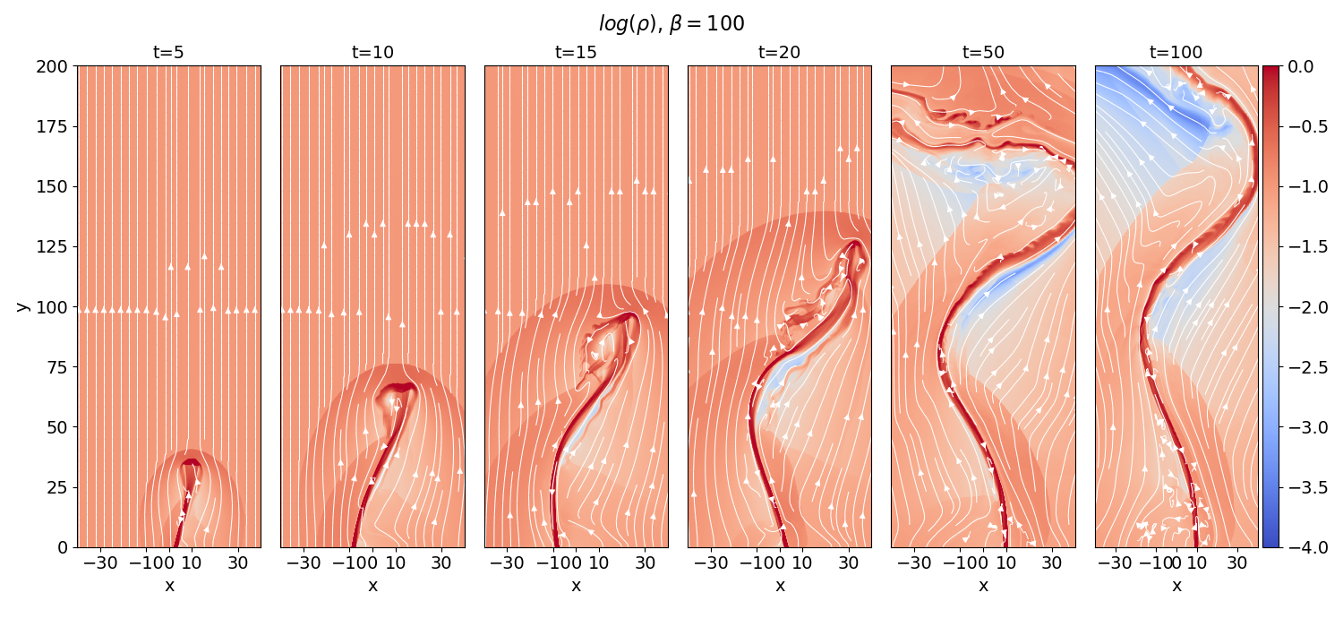
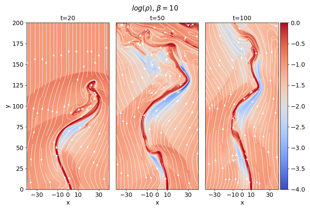
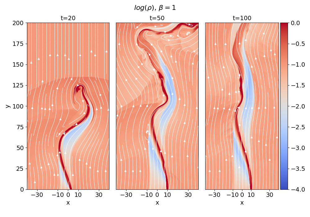
Figure B.1: Time evolution of the magnetized simulation for an orbiting jet nozzle ojP25a10B100 with $\beta=100$ (top), ojP25a10B10 with $\beta=10$ (lower left), and ojP25a10B1 with $\beta=1$ (lower right), all with orbital separation $a=10$ and an orbital period of $P=25$. Shown is the density distribution (colors) and the magnetic field lines (white) for selected the time steps (left to right).

References

- Agudo et al. (2007) Agudo, I., Bach, U., Krichbaum, T. P., et al. 2007, A&A, 476, L17, doi: 10.1051/0004-6361:20078448
- Banerjee et al. (2007) Banerjee, R., Klessen, R. S., & Fendt, C. 2007, ApJ, 668, 1028, doi: 10.1086/521097
- Bate et al. (2000) Bate, M. R., Bonnell, I. A., Clarke, C. J., et al. 2000, MNRAS, 317, 773, doi: 10.1046/j.1365-8711.2000.03648.x
- Begelman et al. (1980) Begelman, M. C., Blandford, R. D., & Rees, M. J. 1980, Nature, 287, 307, doi: 10.1038/287307a0
- Beltrán et al. (2016) Beltrán, M. T., Cesaroni, R., Moscadelli, L., et al. 2016, A&A, 593, A49, doi: 10.1051/0004-6361/201628588
- Biro et al. (1995) Biro, S., Raga, A. C., & Canto, J. 1995, MNRAS, 275, 557, doi: 10.1093/mnras/275.3.557
- Bisikalo et al. (2012) Bisikalo, D. V., Dodin, A. V., Kaigorodov, P. V., et al. 2012, Astronomy Reports, 56, 686, doi: 10.1134/S1063772912090028
- Blandford & Payne (1982) Blandford, R. D., & Payne, D. G. 1982, MNRAS, 199, 883
- Blandford & Znajek (1977) Blandford, R. D., & Znajek, R. L. 1977, MNRAS, 179, 433
- Britzen et al. (2018) Britzen, S., Fendt, C., Witzel, G., et al. 2018, MNRAS, 478, 3199, doi: 10.1093/mnras/sty1026
- Britzen et al. (2021) Britzen, S., Zajaček, M., Popović, L. Č., et al. 2021, MNRAS, 503, 3145, doi: 10.1093/mnras/stab589
- Carroll et al. (2009) Carroll, J. J., Frank, A., Blackman, E. G., Cunningham, A. J., & Quillen, A. C. 2009, ApJ, 695, 1376, doi: 10.1088/0004-637X/695/2/1376
- Casse & Keppens (2002) Casse, F., & Keppens, R. 2002, ApJ, 581, 988, doi: 10.1086/344340
- Chiang & Murray-Clay (2004) Chiang, E. I., & Murray-Clay, R. A. 2004, ApJ, 607, 913, doi: 10.1086/383522
- Cliffe et al. (1996) Cliffe, J. A., Frank, A., & Jones, T. W. 1996, MNRAS, 282, 1114, doi: 10.1093/mnras/282.4.1114
- Colella & Woodward (1984) Colella, P., & Woodward, P. R. 1984, Journal of Computational Physics, 54, 174, doi: 10.1016/0021-9991(84)90143-8
- Crocker et al. (2002) Crocker, M. M., Davis, R. J., Spencer, R. E., et al. 2002, MNRAS, 335, 1100, doi: 10.1046/j.1365-8711.2002.05705.x
- Cunningham et al. (2006) Cunningham, A. J., Frank, A., & Blackman, E. G. 2006, ApJ, 646, 1059, doi: 10.1086/505132
- Dominik et al. (2021) Dominik, R. M., Linhoff, L., Elsässer, D., & Rhode, W. 2021, MNRAS, doi: 10.1093/mnras/stab799
- Duchêne et al. (2002) Duchêne, G., Ghez, A. M., & McCabe, C. 2002, ApJ, 568, 771, doi: 10.1086/338987
- El Mellah et al. (2019) El Mellah, I., Sundqvist, J. O., & Keppens, R. 2019, A&A, 622, L3, doi: 10.1051/0004-6361/201834543
- Erkal et al. (2021) Erkal, J., Dougados, C., Coffey, D., et al. 2021, A&A, 650, A46, doi: 10.1051/0004-6361/202038977
- Fendt (2003) Fendt, C. 2003, A&A, 411, 623, doi: 10.1051/0004-6361:20034154
- Fendt & Zinnecker (1998) Fendt, C., & Zinnecker, H. 1998, A&A, 334, 750
- Ferreira (1997) Ferreira, J. 1997, A&A, 319, 340
- Ferrero et al. (2022) Ferrero, L. V., Günthardt, G., García, L., et al. 2022, A&A, 657, A110, doi: 10.1051/0004-6361/202142421
- Hawley et al. (2015) Hawley, J. F., Fendt, C., Hardcastle, M., Nokhrina, E., & Tchekhovskoy, A. 2015, Space Sci. Rev., 191, 441, doi: 10.1007/s11214-015-0174-7
- Herbst et al. (1996) Herbst, T. M., Beckwith, S. V. W., Glindemann, A., et al. 1996, AJ, 111, 2403, doi: 10.1086/117974
- Hirano & Machida (2019) Hirano, S., & Machida, M. N. 2019, MNRAS, 485, 4667, doi: 10.1093/mnras/stz740
- Hirth et al. (1997) Hirth, G. A., Mundt, R., & Solf, J. 1997, A&AS, 126, 437, doi: 10.1051/aas:1997275
- Hollis & Michalitsianos (1993) Hollis, J. M., & Michalitsianos, A. G. 1993, ApJ, 411, 235, doi: 10.1086/172822
- Hull et al. (2013) Hull, C. L. H., Plambeck, R. L., Bolatto, A. D., et al. 2013, ApJ, 768, 159, doi: 10.1088/0004-637X/768/2/159
- Jaiswal et al. (2019) Jaiswal, S., Mohan, P., An, T., & Frey, S. 2019, ApJ, 873, 11, doi: 10.3847/1538-4357/ab0176
- Jensen & Akeson (2014) Jensen, E. L. N., & Akeson, R. 2014, Nature, 511, 567, doi: 10.1038/nature13521
- Johnson et al. (2004) Johnson, J. A., Marcy, G. W., Hamilton, C. M., Herbst, W., & Johns-Krull, C. M. 2004, AJ, 128, 1265, doi: 10.1086/422735
- Johnson & Winn (2004) Johnson, J. A., & Winn, J. N. 2004, AJ, 127, 2344, doi: 10.1086/382520
- Johnston et al. (2003) Johnston, K. J., Gaume, R. A., Fey, A. L., de Vegt, C., & Claussen, M. J. 2003, AJ, 125, 858, doi: 10.1086/345727
- Karovska et al. (2010) Karovska, M., Gaetz, T. J., Carilli, C. L., et al. 2010, ApJ, 710, L132, doi: 10.1088/2041-8205/710/2/L132
- Kato & Hachisu (2003) Kato, M., & Hachisu, I. 2003, ApJ, 587, L39, doi: 10.1086/375043
- Keppens et al. (2008) Keppens, R., Meliani, Z., van der Holst, B., & Casse, F. 2008, A&A, 486, 663, doi: 10.1051/0004-6361:20079174
- Kharb et al. (2017) Kharb, P., Lal, D. V., & Merritt, D. 2017, Nature Astronomy, 1, 727, doi: 10.1038/s41550-017-0256-4
- Lebedev et al. (2004) Lebedev, S. V., Ampleford, D., Ciardi, A., et al. 2004, ApJ, 616, 988, doi: 10.1086/423730
- Lee et al. (2009) Lee, C., Hirano, N., Palau, A., et al. 2009, ApJ, 699, 1584, doi: 10.1088/0004-637X/699/2/1584
- Lee et al. (2015) Lee, C.-F., Hirano, N., Zhang, Q., et al. 2015, ApJ, 805, 186, doi: 10.1088/0004-637X/805/2/186
- Londrillo & del Zanna (2004) Londrillo, P., & del Zanna, L. 2004, Journal of Computational Physics, 195, 17, doi: 10.1016/j.jcp.2003.09.016
- Margon et al. (1979) Margon, B., Ford, H. C., Grandi, S. A., & Stone, R. P. S. 1979, ApJ, 233, L63, doi: 10.1086/183077
- Masciadri & Raga (2002) Masciadri, E., & Raga, A. C. 2002, ApJ, 568, 733, doi: 10.1086/338767
- McKee & Ostriker (2007) McKee, C. F., & Ostriker, E. C. 2007, ARA&A, 45, 565, doi: 10.1146/annurev.astro.45.051806.110602
- McLoughlin et al. (2021) McLoughlin, D., Blundell, K. M., Lee, S., & McCowage, C. 2021, MNRAS, 503, 704, doi: 10.1093/mnras/stab581
- Mellah et al. (2019) Mellah, I. E., Sander, A. A. C., Sundqvist, J. O., & Keppens, R. 2019, IAU Symposium, 346, 34, doi: 10.1017/S1743921318008414
- Melnikov et al. (2018) Melnikov, S., Stute, M., & Eislöffel, J. 2018, A&A, 612, A77, doi: 10.1051/0004-6361/201731749
- Mignone et al. (2007) Mignone, A., Bodo, G., Massaglia, S., et al. 2007, ApJS, 170, 228, doi: 10.1086/513316
- Mignone et al. (2005) Mignone, A., Massaglia, S., & Bodo, G. 2005, Space Sci. Rev., 121, 21, doi: 10.1007/s11214-006-3588-4
- Millas et al. (2019) Millas, D., Porth, O., & Keppens, R. 2019, in JET Simulations, Experiments, and Theory: Ten Years After JETSET. What Is Next?, ed. C. Sauty, Vol. 55, 71, doi: K55-78716
- Mioduszewski et al. (2004) Mioduszewski, A. J., Rupen, M. P., Walker, R. C., Schillemat, K. M., & Taylor, G. B. 2004, in AAS/High Energy Astrophysics Division #8, AAS/High Energy Astrophysics Division, 29.03
- Monceau-Baroux et al. (2014) Monceau-Baroux, R., Porth, O., Meliani, Z., & Keppens, R. 2014, in The X-ray Universe 2014, ed. J.-U. Ness, 147
- Monceau-Baroux et al. (2015) Monceau-Baroux, R., Porth, O., Meliani, Z., & Keppens, R. 2015, A&A, 574, A143, doi: 10.1051/0004-6361/201425015
- Mundt et al. (1990) Mundt, R., Buehrke, T., Solf, J., Ray, T. P., & Raga, A. C. 1990, A&A, 232, 37
- Mundt et al. (2010) Mundt, R., Hamilton, C. M., Herbst, W., Johns-Krull, C. M., & Winn, J. N. 2010, ApJ, 708, L5, doi: 10.1088/2041-8205/708/1/L5
- Noriega-Crespo et al. (2020) Noriega-Crespo, A., Raga, A. C., Lora, V., & Rodríguez-Ramírez, J. C. 2020, Rev. Mexicana Astron. Astrofis., 56, 29, doi: 10.22201/ia.01851101p.2020.56.01.05
- Papaloizou & Terquem (1995) Papaloizou, J. C. B., & Terquem, C. 1995, MNRAS, 274, 987
- Paron et al. (2016) Paron, S., Fariña, C., & Ortega, M. E. 2016, A&A, 593, A132, doi: 10.1051/0004-6361/201628495
- Podio et al. (2016) Podio, L., Codella, C., Gueth, F., et al. 2016, A&A, 593, L4, doi: 10.1051/0004-6361/201628876
- Pudritz & Norman (1983) Pudritz, R. E., & Norman, C. A. 1983, ApJ, 274, 677, doi: 10.1086/161481
- Pudritz & Ray (2019) Pudritz, R. E., & Ray, T. P. 2019, Frontiers in Astronomy and Space Sciences, 6, 54, doi: 10.3389/fspas.2019.00054
- Raga et al. (1993) Raga, A. C., Canto, J., & Biro, S. 1993, MNRAS, 260, 163, doi: 10.1093/mnras/260.1.163
- Roland et al. (2013) Roland, J., Britzen, S., Caproni, A., et al. 2013, A&A, 557, A85, doi: 10.1051/0004-6361/201219165
- Sheikhnezami & Abgharian-Afoushteh (2019) Sheikhnezami, S., & Abgharian-Afoushteh, M. 2019, ApJ, 883, 160, doi: 10.3847/1538-4357/ab39e2
- Sheikhnezami & Fendt (2015) Sheikhnezami, S., & Fendt, C. 2015, ApJ, 814, 113, doi: 10.1088/0004-637X/814/2/113
- Sheikhnezami & Fendt (2018) —. 2018, ApJ, 861, 11, doi: 10.3847/1538-4357/aac5dc
- Sheikhnezami & Fendt (2022) —. 2022, ApJ, 925, 161, doi: 10.3847/1538-4357/ac3f31
- Shepherd et al. (2000) Shepherd, D. S., Yu, K. C., Bally, J., & Testi, L. 2000, ApJ, 535, 833, doi: 10.1086/308873
- Sillanpaa et al. (1988) Sillanpaa, A., Haarala, S., Valtonen, M. J., Sundelius, B., & Byrd, G. G. 1988, ApJ, 325, 628, doi: 10.1086/166033
- Solf & Ulrich (1985) Solf, J., & Ulrich, H. 1985, A&A, 148, 274
- Stepanovs & Fendt (2014) Stepanovs, D., & Fendt, C. 2014, ApJ, 793, 31, doi: 10.1088/0004-637X/793/1/31
- Stepanovs & Fendt (2016) —. 2016, ApJ, 825, 14, doi: 10.3847/0004-637X/825/1/14
- Stepanovs et al. (2014) Stepanovs, D., Fendt, C., & Sheikhnezami, S. 2014, ApJ, 796, 29, doi: 10.1088/0004-637X/796/1/29
- Stone & Norman (1993a) Stone, J. M., & Norman, M. L. 1993a, ApJ, 413, 198, doi: 10.1086/172988
- Stone & Norman (1993b) —. 1993b, ApJ, 413, 210, doi: 10.1086/172989
- Targon et al. (2011) Targon, C. G., Rodrigues, C. V., Cerqueira, A. H., & Hickel, G. R. 2011, ApJ, 743, 54, doi: 10.1088/0004-637X/743/1/54
- Uchida & Shibata (1985) Uchida, Y., & Shibata, K. 1985, PASJ, 37, 515
- Valtonen et al. (2016) Valtonen, M. J., Zola, S., Ciprini, S., et al. 2016, ApJ, 819, L37, doi: 10.3847/2041-8205/819/2/L37
- Warner (1995) Warner, B. 1995, Cataclysmic variable stars, Vol. 28
- Winn et al. (2004) Winn, J. N., Holman, M. J., Johnson, J. A., Stanek, K. Z., & Garnavich, P. M. 2004, ApJ, 603, L45, doi: 10.1086/383089
- Woo et al. (2014) Woo, J.-H., Cho, H., Husemann, B., et al. 2014, MNRAS, 437, 32, doi: 10.1093/mnras/stt1846
- Zamanov et al. (2005) Zamanov, R., Bode, M. F., Marziani, R., et al. 2005, in American Institute of Physics Conference Series, Vol. 797, Interacting Binaries: Accretion, Evolution, and Outcomes, ed. L. Burderi, L. A. Antonelli, F. D’Antona, T. di Salvo, G. L. Israel, L. Piersanti, A. Tornambè, & O. Straniero, 655–658, doi: 10.1063/1.2130308
- Zanni et al. (2007) Zanni, C., Ferrari, A., Rosner, R., Bodo, G., & Massaglia, S. 2007, A&A, 469, 811, doi: 10.1051/0004-6361:20066400