A Simple Model for Quantum Gravity:
the one-dimensional case

Abstract

Group theory is used to construct a model for quantum gravity and exact results are obtained in one dimension. Comparison with Regge calculus shows that the results agree in the strong cosmological constant limit for an open curve. In the closed case, the average edge length has a minimum value and this give us a clue for higher dimensions.

Keywords: Quantum Gravity, Group Theory, Regge Calculus

1 Introduction

Consider euclidean gravity in 1D, that is, a curve representing time, $x$. As the intrinsic curvature is zero, we will work with the action

$$S=\lambda\int dx\,\sqrt{|\det g|}=\lambda L,$$

where $\lambda$ is the cosmological constant, $L=\int dx\,\sqrt{|\det g|}$ is the total length and we set $\hbar=c=1$.

Since the only observable here is $L$, we are interested in your average value, $\langle L\rangle$. So we have to calculate the partition function

$$Z=\int Dg\,\exp(-S)=\int Dg\,\exp(-\lambda L)$$ (1)

and then take the derivative

$$\langle L\rangle=-\frac{1}{Z}\frac{dZ}{d\lambda}=-\frac{d(\ln Z)}{d\lambda},$$ (2)

where $g$ is the metric, $Dg$ is a measure, and $Z$ is a path integral, that is, a sum over all possible metrics. Even in 1D, to calculate $Z$ exactly is tricky (see Sec. 2.2) and we often rely on numerical methods.

One of the most important examples of numerical calculation is the quantum Regge calculus [1], where they approximate a curve by $N$ edges and use their lengths, $l_{n}$ for $n=1,2,\ldots N$, as the integration variables.

Usually, they choose the measure $\prod_{n=1}^{N}dl_{n}l_{n}^{\sigma+1}$ with some appropriate power $\sigma>-2$ to make the integrals convergent. They also work with an infinity interval $\epsilon\leq l_{n}<\infty$, where $\epsilon>0$ is an ultraviolet cutoff.

In order to obtain the continuum limit, they make $N$ as big as they can and $\epsilon$ small as they can too. And in higher dimensions, they have to guarantee that the triangle inequalities between the edges are satisfied. This is put in the measure by hand.

There are other choices for the measure, including non-local measures, but we beg to disagree with them. We believe that the measure must be unique (up to normalization) as the Haar measure of group theory.

2 One-Dimensional Model

Instead of working with lengths and their infinity intervals, inequalities, etc. We would like to use angles and their finite intervals, which in 1D is related to the rotation group, SO(2), or equivalently the U(1) group.

To do this, we will associate an angle, $\phi_{n}$, for each pair of equal lengths, $l_{n}/2$, in a circle of radius $\ell$, as in the open polygonal line represented in Fig. (1).

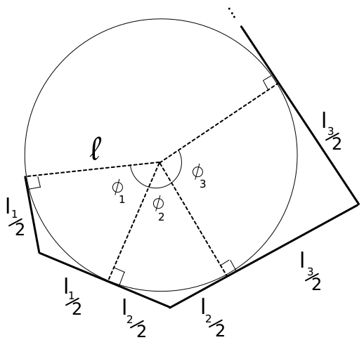
Figure 1: Open polygon tangent to the U(1) circle.

Notice that we can align this polygon into a straight line or approximate it to any curve we want, but this is just the extrinsic curvature.

2.1 Open Case

For the moment, the sum of the angles are not constrained, the polygonal line can turn around the circle freely. But each angle is restricted to $0\leq\phi_{n}<\pi$ because the length $l_{n}=2\ell\tan(\phi_{n}/2)$ lies in the interval $[0,\infty)$.

Thus we have the (unique) normalized Haar measure

$$\prod_{n=1}^{N}\left(\int_{0}^{\pi}\frac{d\phi_{n}}{\pi}\right)$$

and the total length or perimeter is given by

$$L=\sum_{n=1}^{N}l_{n}=2\ell\sum_{n=1}^{N}\tan\frac{\phi_{n}}{2}.$$ (3)

Obviously, we can choose the interval to be $[-\pi,\pi)$, or $[0,2\pi)$, etc. But we don’t want to complicate things at this stage by using the absolute value $|\tan(\phi_{n}/2)|$ in $L$ (see Sec. 2.2).

Since the angles are independent, this quantum curve is very easy to calculate. The partition function, Eq. (1), separates into $N$ copies of the same integral [2]

$$Z=\prod_{n=1}^{N}\left(\int_{0}^{\pi}\frac{d\phi_{n}}{\pi}\right)\exp(-\lambda L)=\left\{\int_{0}^{\pi}\frac{d\phi}{\pi}\exp\left[-2\lambda\ell\tan\left(\frac{\phi}{2}\right)\right]\right\}^{N}$$

$$=\left\{\frac{2}{\pi}[\operatorname{ci}(2\lambda\ell)\sin(2\lambda\ell)-\operatorname{si}(2\lambda\ell)\cos(2\lambda\ell)]\right\}^{N},$$ (4)

where

$$\operatorname{si}(x)=\int_{0}^{x}\frac{\sin t}{t}dt-\frac{\pi}{2},\quad\text{and}\quad\operatorname{ci}(x)=\gamma+\ln x+\int_{0}^{x}\frac{\cos t-1}{t}dt,$$

are the sine and cosine integrals, respectively. Here $\gamma=0.577\ldots$ is the Euler constant.

Thus the average edge length $\langle l\rangle=\langle L\rangle/N$ is

$$\langle l\rangle=2\ell\left[\frac{1+\text{ti}(2\lambda\ell)\tan(2\lambda\ell)}{\text{ti}(2\lambda\ell)-\tan(2\lambda\ell)}\right],$$ (5)

where we have defined $\text{ti}(x)=\operatorname{si}(x)/\operatorname{ci}(x)$.

Eq. (5) is exact, see Fig. (2), but it can be approximated, using series [2] for $\operatorname{si}(x)$ and $\operatorname{ci}(x)$, as

$$\langle l\rangle\approx\begin{cases}-4\ell[\gamma+\ln(2\lambda\ell)]/\pi,&\lambda\ell\ll 1,\\ 1/\lambda,&\lambda\ell\gg 1.\end{cases}$$ (6)

In the strong approximation, $\lambda\ell\gg 1$, Eq. (6) is equal to $\langle l\rangle=(2+\sigma)/\lambda$, with the measure $\prod_{n}dl_{n}l_{n}^{\sigma+1}$ used in Regge calculus [1], for $\sigma=-1$.

In view of the Wigner-Inönü contraction, it is easy to understand what is happening here: as the radius, $\ell$, of the U(1) circle becomes greater, the length of the arc, $\ell\phi_{n}$, becomes more and more close to the edge length, $l_{n}$, that is associated with the translation group, $T^{1}$. Thus $d\phi_{n}\approx dl_{n}/\ell$ and we get $\sigma\approx-1$.

Note that $\ell$ has nothing to do with the continuum limit, it is a constant related to the U(1) manifold and we do not take this to zero. The continuum limit is obtained solely as the number of edges, $N$, goes to infinity. Since we have defined $\langle l\rangle=\langle L\rangle/N$, then $N$ disappears, as in Statistical Mechanics.

In this aspect, quantum gravity is completely different from quantum field theory on a lattice, where we make $N\to\infty$ simultaneously with the lattice size $a\to 0$. Remember that in QFT all lengths $l_{n}$ are equal to the lattice size, $a$.

However in quantum gravity we don’t have control of the lengths, they fluctuate from a minimum value to infinity, see Fig. (2).

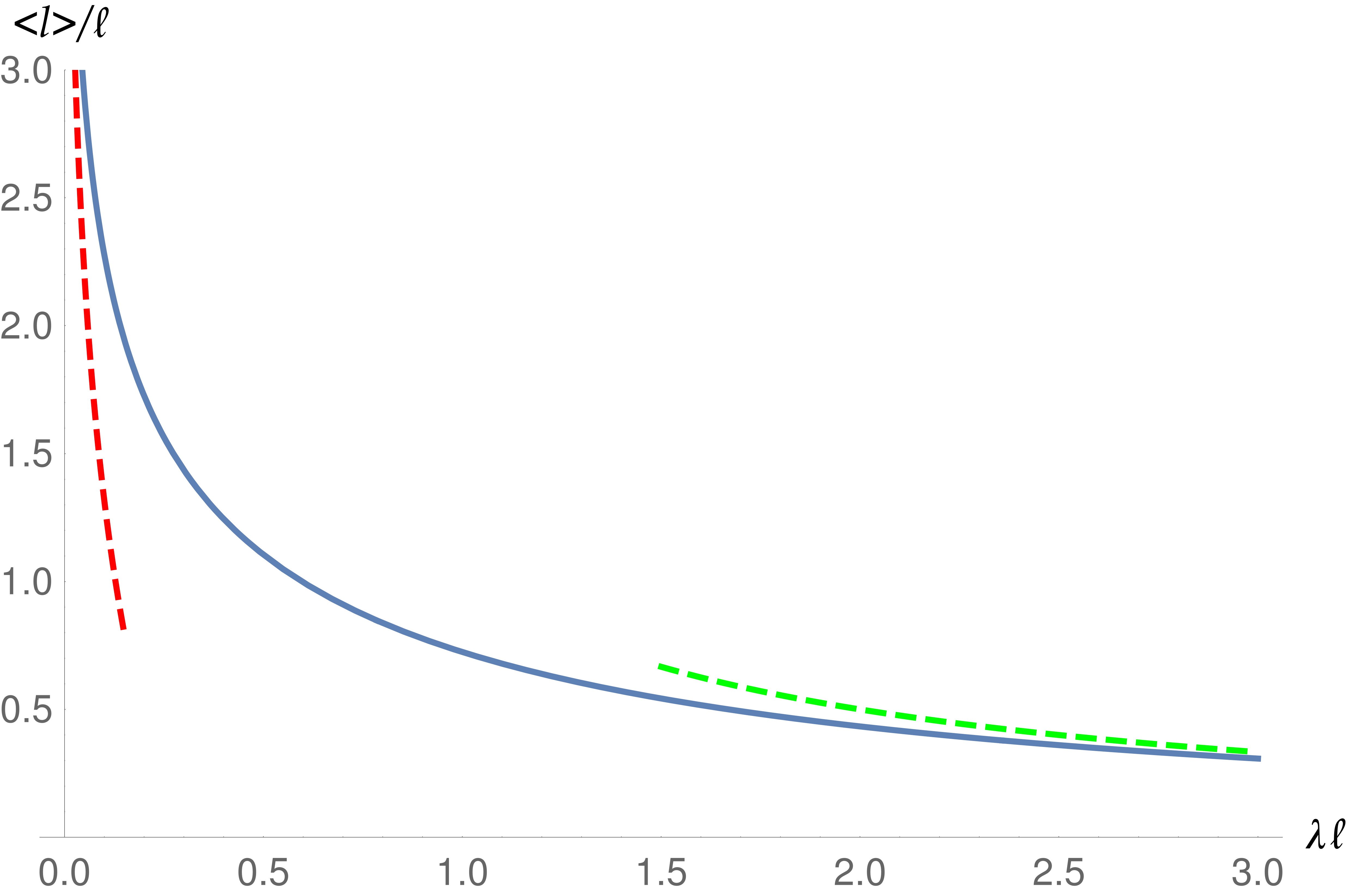
Figure 2: Average edge length for the exact value, Eq. (5), is plotted as a continuous curve (in blue) together with the approximations, Eq. (6), for weak (in red) and strong cosmological constant (in green).

2.2 Closed Case

A more complicated problem, but a little bit more realistic than the open case, is the closed polygon, with the topology of the circle $S^{1}$, because of the constraint

$$\sum_{n=1}^{N}\phi_{n}=2\pi,$$ (7)

where $N=3,4,5\ldots$ to close the triangle, quadrilateral, etc. For simplicity, we will restrict the problem to just one wind around the circle.

In this case, the partition function, Eq. (4), is replaced by

$$Z={\cal N}\prod_{n=1}^{N}\left(\int_{0}^{\pi}\frac{d\phi_{n}}{\pi}\right)\delta\left(\sum_{n=1}^{N}\phi_{n}-2\pi\right)\exp\left(-2\lambda\ell\sum_{n=1}^{N}\tan\frac{\phi_{n}}{2}\right),$$ (8)

where ${\cal N}$ is a normalization constant. For $N=3,4,5,\ldots$ edges, one can choose ${\cal N}=2\pi,\frac{3\pi}{2},\frac{24\pi}{11},\ldots$ to make $Z=1$ when $\lambda=0$. Obviously, the observable $\langle l\rangle$ do not depends on ${\cal N}$.

The first problem is that we can not use perturbation theory here. Usually, we expand the exponential in Taylor series, using the dimensionless coupling, $\lambda\ell$. But the integral of the tangent function diverges $\int_{0}^{\pi}d\phi\,\tan(\phi/2)=\infty$. (Remember that the lengths are not restricted, only the sum of the angles is).

One can try to regularize this integral choosing a cutoff. For example, reducing the interval from $[0,\pi]$ to $[0,\pi-\epsilon]$ with some small $\epsilon>0$. But at each order in $\lambda\ell$ the divergence becomes more severe. This situation is similar to the QFT versions of gravity [3], where the degree of divergence increase order by order.

Since we are using the Haar measure, a natural alternative to perturbation theory is to use the character expansion for these functions. Nevertheless, the well-known character expansion for the delta function

$$\delta(\phi)=\frac{1}{2\pi}\sum_{p=-\infty}^{\infty}\chi_{p}(\phi),$$ (9)

where $\chi_{p}(\phi)=\exp(-ip\phi)$ and $p\in\mathbb{Z}$, doesn’t work when there are several variables and a constant.

One way out is to expand the delta function using a product of characters

$$\delta\left(\sum_{n}\phi_{n}-2\pi\right)=\sum_{p,q,\ldots,r}c_{pq\ldots r}\chi_{p}(\phi_{1})\chi_{q}(\phi_{2})\ldots\chi_{r}(\phi_{N}),$$ (10)

where the coefficients $c_{pq\ldots r}$ can be found, using the orthogonality relation

$$\int_{-\pi}^{\pi}\frac{d\phi}{2\pi}\chi_{p}(\phi)\chi_{q}^{*}(\phi)=\delta_{pq},$$ (11)

to be

$$c_{pq\ldots r}=\int_{-\pi}^{\pi}\frac{d\phi_{1}}{2\pi}\int_{-\pi}^{\pi}\frac{d\phi_{2}}{2\pi}\ldots\int_{-\pi}^{\pi}\frac{d\phi_{N}}{2\pi}\delta\left(\sum_{n}\phi_{n}-2\pi\right)\chi_{p}^{*}(\phi_{1})\chi_{q}^{*}(\phi_{2})\ldots\chi_{r}^{*}(\phi_{N}).$$

These integrals are not hard to calculate, because the first integral turns the delta into a Heaviside function $H$ and then the interval is reduced.

For example, with $N=3$ we have

$$c_{pqr} =\int_{-\pi}^{\pi}\frac{d\phi_{1}}{2\pi}\int_{-\pi}^{\pi}\frac{d\phi_{2}}{2\pi}\int_{-\pi}^{\pi}\frac{d\phi_{3}}{2\pi}\delta(\phi_{1}+\phi_{2}+\phi_{3}-2\pi)\chi_{p}^{*}(\phi_{1})\chi_{q}^{*}(\phi_{2})\chi_{r}^{*}(\phi_{3})$$

$$=\frac{1}{8\pi^{3}}\int_{-\pi}^{\pi}d\phi_{1}\chi_{p}^{*}(\phi_{1})\int_{-\pi}^{\pi}d\phi_{2}\chi_{q}^{*}(\phi_{2})\exp[-ir(\phi_{1}+\phi_{2})]H(\phi_{1}+\phi_{2}-\pi)$$

$$=\frac{1}{8\pi^{3}}\int_{0}^{\pi}d\phi_{1}\exp[i(p-r)\phi_{1}]\int_{\pi-\phi_{1}}^{\pi}d\phi_{2}\exp[i(q-r)\phi_{2}]$$

$$=\frac{i(-1)^{q-r}}{8\pi^{3}(q-r)}\int_{0}^{\pi}d\phi_{1}\{\exp[i(p-q)\phi_{1}]-\exp[i(p-r)\phi_{1}]\}$$

$$=\frac{(p-q)(-1)^{p-q}+(q-r)(-1)^{q-r}+(r-p)(-1)^{r-p}}{8\pi^{3}(p-q)(q-r)(r-p)}.$$ (12)

Note the cyclic symmetry between the indices $p$, $q$, and $r$. Care must be taken with Eq. (12) when a pair or triple of indices are equal, this case must be seen as a limit.

Similarly, for each exponential we have the character expansion

$$\exp[-2\lambda\ell|\tan(\phi/2)|]=\sum_{p=-\infty}^{\infty}d_{p}\chi_{p}(\phi),$$ (13)

where the coefficients $d_{p}$ are

$$d_{p}=\int_{-\pi}^{\pi}\frac{d\phi}{2\pi}\exp[-2\lambda\ell|\tan(\phi/2)|]\chi_{p}^{*}(\phi),$$

which is valid for $\lambda\geq 0$. Notice that we are working now with an absolute value, because the orthogonality relation, Eq. (11), only works with the complete interval $[-\pi,\pi)$, or $[0,2\pi)$, etc. However, by the symmetry, this equation can be reduced from a complex Fourier integral to a cosine Fourier integral without the modulus

$$d_{p}=\int_{0}^{\pi}\frac{d\phi}{\pi}\exp[-2\lambda\ell\tan(\phi/2)]\cos(p\phi),$$ (14)

which shows that $d_{-p}=d_{p}$ and $d_{p}$ is real.

To evaluate Eq. (14) we will use a representation for the exponential function as an inverse Mellin transform [4] (this will be useful for 2D and higher)

$$\exp(-x)=\int_{\sigma-i\infty}^{\sigma+i\infty}\frac{dz}{2\pi i}\frac{\Gamma(z)}{x^{z}},$$

where $\sigma=\Re(z)>0$.

Now we change the order of integration

$$d_{p}=\int_{\sigma-i\infty}^{\sigma+i\infty}\frac{dz}{2\pi i}\frac{\Gamma(z)}{(2\lambda\ell)^{z}}\int_{0}^{\pi}\frac{d\phi}{\pi}\frac{\cos(p\phi)}{\tan^{z}(\phi/2)}$$ (15)

and the $\phi$ integral is

$$\int_{0}^{\pi}\frac{d\phi}{\pi}\frac{\cos(p\phi)}{\tan^{z}(\phi/2)}=\sec\left(\frac{\pi z}{2}\right)f_{p}(z),$$ (16)

valid for $0<\sigma<1$, where $f_{p}(z)=f_{-p}(z)$ is a polynomial

$$f_{0}(z)=1,\;f_{1}(z)=z,\;f_{2}(z)=z^{2},\;f_{3}(z)=\frac{2z^{3}+z}{3},\;f_{4}(z)=\frac{z^{4}+2z^{2}}{3},\;\ldots$$

obtained by the Chebyshev polynomial of the first kind $T_{2p}(x)$ with $x^{2n}$ replaced by $(z+1)(z+3)...(z+2n-1)/(2^{n}n!)$ or more explicitly

$$f_{p}(z)=\begin{cases}1,&p=0\\ \sum_{k=0}^{p}\frac{(-1)^{k}p(z+1)2^{-2k+2p-1}(-k+2p-1)!\left(\frac{z+3}{2}\right)_{-k+p-1}}{k!(p-k)!(2p-2k)!},&p\geq 1\end{cases}$$

where $(x)_{n}=\Gamma(x+n)/\Gamma(x)$ is the Pochhammer symbol and the last expression can be written as a hypergeometric function $\frac{2^{2p-1}}{p!}\left(\frac{z+1}{2}\right)_{p}{}_{3}F_{2}\left(\frac{1}{2}-p,-p,-p;1-2p,\frac{1}{2}-p-\frac{z}{2};1\right)$, but we will not use them.

Substituting Eq. (16) in Eq. (15), we obtain inverse Mellin transforms

$$\int_{\sigma-i\infty}^{\sigma+i\infty}\frac{dz}{2\pi i}\frac{\Gamma(z)\sec(\pi z/2)z^{n}}{x^{z}}=\begin{cases}\frac{2}{\pi}(\operatorname{ci}x\sin x-\operatorname{si}x\cos x),&n=0\\ -\frac{2x}{\pi}(\operatorname{ci}x\cos x+\operatorname{si}x\sin x),&n=1\\ \frac{(-2)^{n}}{\pi^{3/2}}G_{n,n+2}^{4,n-1}\biggl{(}\frac{x}{2},\frac{1}{2}|\begin{array}[]{c}0,\ldots,0,\frac{1}{2},0\\ \frac{1}{2},\frac{1}{2},1,1,1,\ldots,1\end{array}\biggr{)},&n\geq 2\end{cases}$$

where $G$ is the generalized Meijer function. So we can read off $d_{p}$ directly from $f_{p}(z)$, for example

$$d_{0}=\frac{2}{\pi}[\operatorname{ci}(2\lambda\ell)\sin(2\lambda\ell)-\operatorname{si}(2\lambda\ell)\cos(2\lambda\ell)],\;d_{1}=-\frac{4\lambda\ell}{\pi}[\operatorname{ci}(2\lambda\ell)\cos(2\lambda\ell)+\operatorname{si}(2\lambda\ell)\sin(2\lambda\ell)],$$

$$d_{2}=-\frac{4}{\pi^{3/2}}G_{2,4}^{3,2}\left(\lambda\ell,\frac{1}{2}|\begin{array}[]{c}0,\frac{1}{2}\\ \frac{1}{2},\frac{1}{2},1,1\end{array}\right),\;d_{3}=\frac{16}{3\pi^{3/2}}G_{3,5}^{3,3}\left(\lambda\ell,\frac{1}{2}|\begin{array}[]{c}0,0,\frac{1}{2}\\ \frac{1}{2},\frac{1}{2},1,1,1\end{array}\right)$$ (21)

$$-\frac{4\lambda\ell}{3\pi}[\operatorname{ci}(2\lambda\ell)\cos(2\lambda\ell)+\operatorname{si}(2\lambda\ell)\sin(2\lambda\ell)],\;\ldots$$ (22)

Observe that $d_{0}$ has appeared before, in the open case, Eq. (4).

Substituting the expansions from Eqs. (10) and (13) into the partition function, Eq. (8), and using the orthogonality relation, Eq. (11), gives us the exact answer to the problem of the closed quantum line

$$Z={\cal N}\sum_{p,q,\ldots,r}c_{pq\ldots r}d_{p}d_{q}\ldots d_{r}.$$ (23)

In Fig. (3) we plotted the average edge length, $\langle l\rangle=-(1/N)d(\ln Z)/d\lambda$, using the exact answer, Eq. (23), for the $N=3$ case. Just a few terms are necessary, because of the rapid convergence of Eq. (23).

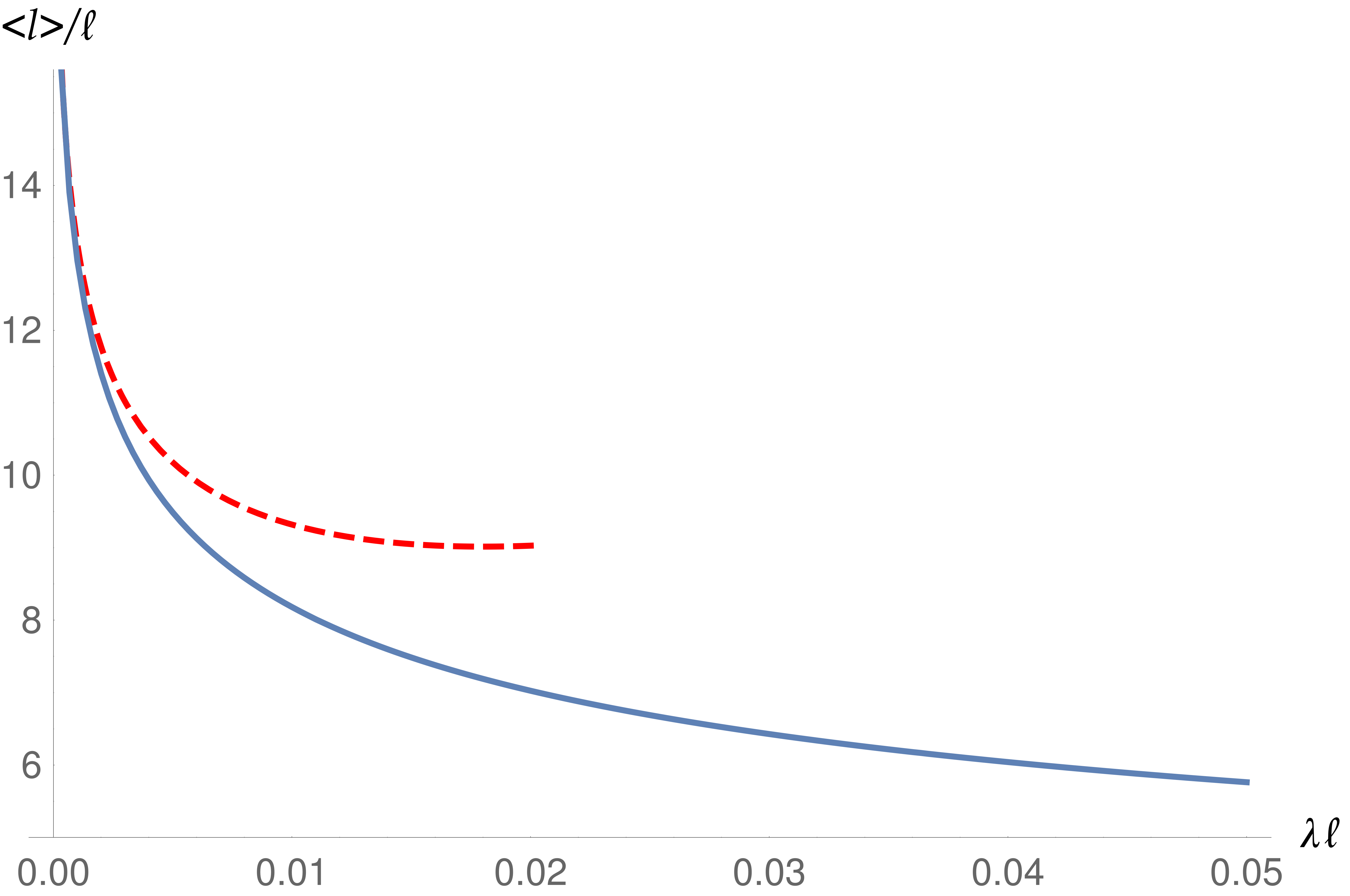
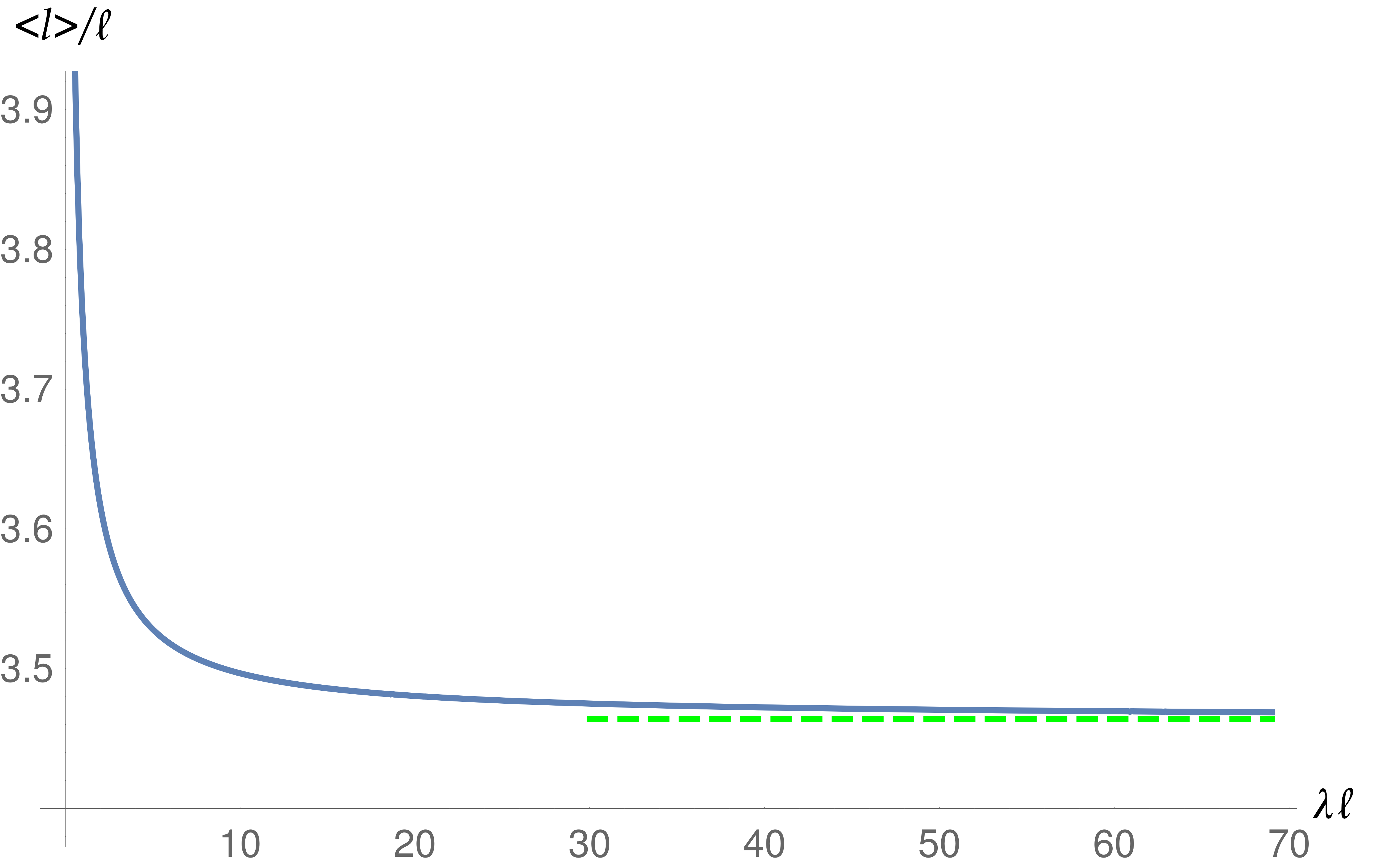
Figure 3: Average edge length for the exact value, Eq. (23), is plotted as a continuous curve (in blue) together with the approximations for weak (left figure, Eq. (24), in red) and strong cosmological constant (right figure, Eq. (25), in green). We split the figure in two figures because they are far away in the $\lambda\ell$ range.

The approximations for weak and strong cosmological constant are calculated in the next sections.

2.2.1 Weak Cosmological Constant

For $\lambda\ell\ll 1$ we can approximate the coefficients $d_{p}$ as (see appendix A)

$$d_{p}\approx\delta_{p0}+\frac{4\lambda\ell(-1)^{p}}{\pi}\left[\gamma-1+\ln(2\lambda\ell)+\sum_{s=0}^{|p|-1}\frac{1}{2[s/2]+1}\right].$$

Substituting this approximation in Eq. (23) and keeping terms up to order $\lambda\ell$, again for $N=3$, we get

$$Z=16\pi\sum_{p,q,r}c_{pqr}d_{p}d_{q}d_{r}\approx 1+3\sum_{p}16\pi c_{p00}\frac{4\lambda\ell(-1)^{p}}{\pi}\left[\gamma-1+\ln(2\lambda\ell)+\sum_{s=0}^{|p|-1}\frac{1}{2[s/2]+1}\right],$$

where

$$c_{p00}=\frac{1}{16\pi}\begin{cases}1,&p=0\\ 2[(-1)^{p}-1]/p^{2}\pi^{2}-i2(-1)^{p}/p\pi,&p\neq 0\end{cases}$$

from Eq. (12).

Since $Z$ is real, the imaginary part cancel out and the real part contributes only when $p$ is odd, thus

$$Z\approx 1+\frac{12\lambda\ell}{\pi}[\gamma-1+\ln(2\lambda\ell)]\left[1+\frac{8}{\pi^{2}}\sum_{t=0}^{\infty}\frac{1}{(2t+1)^{2}}\right]$$

$$+\frac{96\lambda\ell}{\pi^{3}}\sum_{t=0}^{\infty}\frac{1}{(2t+1)^{2}}\sum_{s=0}^{2t}\frac{1}{2[s/2]+1}$$

$$\approx 1+\frac{24\lambda\ell}{\pi}[\gamma-1+\ln(4\lambda\ell)],$$

where we have used (see appendix B)

$$\sum_{t=0}^{\infty}\frac{1}{(2t+1)^{2}}=\frac{\pi^{2}}{8},\qquad\sum_{t=0}^{\infty}\frac{1}{(2t+1)^{2}}\sum_{s=0}^{2t}\frac{1}{2[s/2]+1}=\frac{\pi^{2}}{4}\ln 2.$$

Therefore the average edge length is

$$\frac{\langle l\rangle}{\ell}\approx-\frac{8[\gamma+\ln(4\lambda\ell)]}{\pi+24\lambda\ell[\gamma-1+\ln(4\lambda\ell)]}$$ (24)

which is the curve plotted in red in Fig. (3).

2.2.2 Strong Cosmological Constant

For $\lambda\ell\gg 1$ the partition function is dominated by configurations that minimize the total length, $L$. So we have to find the minimum of Eq. (3) with the constraint, Eq. (7), that is,

$$\vec{\nabla}L(\phi_{1},\ldots,\phi_{N})=\alpha\vec{\nabla}C(\phi_{1},\ldots,\phi_{N}),$$

where

$$C(\phi_{1},\ldots,\phi_{N})=\sum_{n}\phi_{n}-2\pi$$

and $\alpha$ is a Lagrange multiplier. And the answer is trivial: all angles are equal, thus $\phi_{n}=2\pi/N$ and $L_{\text{min}}=2\ell N\tan(\pi/N)$ is the minimum perimeter. Clearly,

$$\frac{\langle l_{\text{min}}\rangle}{\ell}=2\tan\left(\frac{\pi}{N}\right)$$ (25)

is the minimum average edge length for the polygon with $N$ sides.

The case of the triangle, $N=3$, is plotted in Fig. (3), as a constant curve in green, where $\langle l_{\text{min}}\rangle/\ell=2\sqrt{3}\approx 3.464\ldots$ which is the length of an equilateral triangle with an inscribed circle of radius $\ell$.

Note that the closed polygon is different from the open case, where the open polygon could shrink to zero length. Here the constraint fixes a minimal length.

3 Conclusions

A path integral, as in Eq. (1), is a “sum over paths”, that in the case of quantum gravity means an integration in the space of all possible metrics, $g$. In a 1D lattice, with edge lengths $l_{n}$ for $n=1,\ldots,N$, since $g$ has only one component, $g=(g_{11})$, we can choose $g_{11}(l_{n})$ to be the same as the length squared, that is, $g_{11}(l_{n})=l_{n}^{2}$. Therefore, it is natural to consider integrals of $l_{n}$.

As far as we know, there is no general consensus about the measure, $Dg=dl_{n}f(l_{n})$, where $f(l_{n})$ is a function of only $l_{n}$ for a local measure. For example, in Regge calculus [1] they choose $f(l_{n})=l_{n}^{\sigma+1}$ for some number $\sigma$. Besides the ambiguity in the value of $\sigma$, there are some difficulties such as the triangle inequalities, ultraviolet cutoff, etc.

The main idea of our simple model is to work with the angles, $\phi_{n}$, and set the unique Haar measure for U(1), which is a compact group. The open polygon was very easy to calculate, Eq. (4). But in the little more realistic example of the closed line, Eq. (8), there was some problems.

The first problem is that we can not use perturbation theory with a Boltzmann weight, $\exp(-\lambda L)=1-\lambda L+\lambda^{2}L^{2}/2+\ldots$, that diverges $\int Dg\,L=\int Dg\,L^{2}=\ldots=\infty$ at each order in $\lambda$. This is similar to the QFT expansions for quantum gravity [3], where we have to absorb a new infinity at each order in Newton’s constant.

Since we are using the Haar measure, an alternative is to expand the Dirac delta function and the Boltzmann weight in characters, $\chi_{p}(\phi_{n})$, but then we have another problem: the global constraint, Eq. (7), involves all the angles $\phi_{n}$ and this can not be treated with the usual delta function expansion, Eq. (9).

To solve this second problem, we use a new expansion, Eq. (10), that multiplies all characters, one for each angle $\phi_{n}$. The result in the closed case is very interesting: the average edge length, $\langle l\rangle=\langle L\rangle/N$, varies from a minimum value, Eq. (25), to infinity, see Fig. (3). This is different from Regge calculus, where $\langle l\rangle\propto 1/\lambda$.

Notice that the radius, $\ell$, of the U(1) circle is related to this minimum average edge length, $\langle l_{\text{min}}\rangle$, which in turn is connected to the configuration of maximum symmetry of the polygon. This give us a hint of what happens in higher dimensions.

For example, in 2D the minimum surface is a regular tetrahedron with a inscribed sphere of radius $\ell$, which can be related to a shell in the SU(2) manifold. In 3D, the SU(2) ball must be used and the radius (not a constant anymore) is related to the height of the solid tetrahedron. And so on…

The 2D case is under study right now and will be published soon. Inclusion of matter and fields can be done in the same way as in Regge calculus [1] and these calculations will be published somewhere.

Finally, one can say that we have to integrate in $\ell$, which bring back the infinities, because the number of independent variables in our model is one less than in Regge calculus [1]. However, in the continuum limit $N\to\infty$ this makes no difference at all.

Appendix A Approximation

For small $x=2\lambda\ell$ the coefficients in Eq. (22) can be approximated to

$$d_{p}\approx\delta_{p0}+\frac{2x(-1)^{p}}{\pi}(\gamma-1+\ln x+S_{p}),$$

where

$$S_{0}=0,\;S_{1}=1,\;S_{2}=2,\;S_{3}=\frac{7}{3},\;S_{4}=\frac{8}{3},\;S_{5}=\frac{43}{15},\;S_{6}=\frac{46}{15},\;S_{7}=\frac{337}{105},\;S_{8}=\frac{352}{105},\;\ldots$$

This sequence can be written as

$$1 =1$$

$$2 =1+1$$

$$\frac{7}{3} =1+1+\frac{1}{3}$$

$$\frac{8}{3} =1+1+\frac{1}{3}+\frac{1}{3}$$

$$\frac{43}{15} =1+1+\frac{1}{3}+\frac{1}{3}+\frac{1}{5}$$

$$\frac{46}{15} =1+1+\frac{1}{3}+\frac{1}{3}+\frac{1}{5}+\frac{1}{5}$$

$$\frac{337}{105} =1+1+\frac{1}{3}+\frac{1}{3}+\frac{1}{5}+\frac{1}{5}+\frac{1}{7}$$

$$\frac{352}{105} =1+1+\frac{1}{3}+\frac{1}{3}+\frac{1}{5}+\frac{1}{5}+\frac{1}{7}+\frac{1}{7}$$

$$\vdots$$

which is equal to

$$S_{p}=\sum_{s=0}^{p-1}\frac{1}{2[s/2]+1},$$ (26)

where $[s/2]$ is the integer part of $s/2$. This is also equivalent to

$$S_{p}=H_{p}+\frac{1}{p}\sum_{s=0}^{p}[(-1)^{s}\Phi(-1,1,s)+\ln 2],$$

where $H_{p}$ is the harmonic number and $\Phi$ is the Lerch transcendent.

Appendix B Double series

To find the sum of $S_{p}/p^{2}$, see Eq. (26), for $p=2t+1$ an odd integer, we note that

$$\sum_{t=0}^{\infty}\frac{S_{2t+1}}{(2t+1)^{2}}=\sum_{t=0}^{\infty}\frac{1}{(2t+1)^{2}}\sum_{s=0}^{2t}\frac{1}{2[s/2]+1}$$

$$=2+\frac{2}{3^{2}}\left(1+\frac{1}{3}\right)+\frac{2}{5^{2}}\left(1+\frac{1}{3}+\frac{1}{5}\right)+\frac{2}{7^{2}}\left(1+\frac{1}{3}+\frac{1}{5}+\frac{1}{7}\right)+\ldots-\left(1+\frac{1}{3^{3}}+\frac{1}{5^{3}}+\frac{1}{7^{3}}+\ldots\right)$$

$$=2\sum_{m=0}^{\infty}\frac{1}{(2m+1)^{2}}\sum_{n=0}^{m}\frac{1}{2n+1}-\sum_{m=0}^{\infty}\frac{1}{(2m+1)^{3}}$$

$$=2\sum_{m=0}^{\infty}\frac{1}{(2m+1)^{2}}\left[\ln 2+\frac{\gamma}{2}+\frac{\psi(m+3/2)}{2}\right]-\frac{7}{8}\zeta(3),$$

where $\psi$ is the digamma function and $\zeta$ is the Riemann zeta function. Using that $\psi(m+3/2)=\psi(m+1/2)+2/(2m+1)$ and [5]

$$\sum_{m=0}^{\infty}\frac{\psi(m+1/2)}{(2m+1)^{2}}=-\frac{1}{8}[\pi^{2}\gamma+7\zeta(3)]$$

we obtain the double series

$$\sum_{t=0}^{\infty}\frac{1}{(2t+1)^{2}}\sum_{s=0}^{2t}\frac{1}{2[s/2]+1}=\frac{\pi^{2}}{4}\ln 2.$$

References

- [1] H. Hamber and R. Williams, Nucl. Phys. B 451 (1995) 305.
- [2] I. Gradshteyn and I. Ryzhik, Table of Integrals, Series, and Products (Academic Press, 2015).
- [3] R. Paszko and A. Accioly, Class. Quant. Grav. 27 (2010) 145012.
- [4] G. Iwata, Prog. Theor. Phys. 24 (1960) 1118.
- [5] Y. Brychkov, Handbook of Special Functions (CRC Press, 2008).