Probability distributions for kinetic roughening in the Kardar-Parisi-Zhang growth with long-range temporal and spatial correlations

Abstract

We investigate numerically the effects of long-range temporal and spatial correlations based on probability distribution of interface width $W(L,t)$ within the early growth regimes in the (1+1)-dimensional Kardar-Parisi-Zhang (KPZ) growth system. Through extensive numerical simulations, we find that long-range temporally correlated noise could not significantly impact the distribution form of interface width. Generally, $W(L,t)$ obeys Tracy-Widom Gaussian symplectic ensembles(TW-GSE) when the temporal correlation exponent $\theta\geq 0$. On the other hand, the effects of long-range spatially correlated noise are evidently different from the temporally correlated case. Our results show that, when the spatial correlation exponent $\rho\leq 0.20$, the distribution form of $W(L,t)$ approaches to TW-GSE, and when $\rho>0.20$, the distribution becomes more asymmetric, leptokurtic, and fat-tailed, and tends to an unknown form, which is similar to Gumbel distribution.

1 Introduction

Nonequilibrium processes are common in nature, which play indispensable roles in many actual physical phenomena, such as kinetic roughening, turbulence, combustion and active matter, among others Barabasi1995 ; Chen2016 ; Veynante2002 . As a typical nonequilibrium system, kinetic roughening has received much attention for several decadesBarabasi1995 ; Kardar1986 ; Family1985 ; Chu2016 ; Halpin1995 . The Kardar-Parisi-Zhang (KPZ) equation, which was originally used to describe kinetic roughening processKardar1986 , is one of the most important nonlinear Langevin-type growth equations in this field, and it can also be observed in many other fieldsBarabasi1995 ; Squizzato2018 ; Kulkarni2013 ; Gladilin2014 ; Altman2015 ; Mathey2015 ; Chen2016 . The KPZ equation in the (1+1)-dimensions readsKardar1986 ,

$$\frac{{\partial{{h}}\left({x,t}\right)}}{{\partial t}}=\nu{\nabla^{2}}h+\frac{\lambda}{2}{\left({\nabla h}\right)^{2}}+\eta\left({x,t}\right),$$ (1)

where $h(x,t)$ is the interface height in position $x$ and time $t$, $\nu$ is the surface tension describing relaxation of the interface, $\lambda$ is the nonlinear coefficient, representing lateral growth, and $\eta(x,t)$ is stochastic force that usually is uncorrelated

$$\left\langle{\eta\left({x,t}\right)\eta\left({x^{\prime},t^{\prime}}\right)}\right\rangle\sim\delta\left({x-x^{\prime}}\right)\delta\left({t-t^{\prime}}\right).$$ (2)

Previous research has indicated that surface roughening processes exhibit scaling behaviorsFamily1985 ; Zhang1990 ; Hentschel1991 ; Hanfei1993 , which are often characterized by the rms fluctuation of surface and interface height. To describe the characteristic of kinetic roughening, one often uses interface width that is defined byBarabasi1995

$${W}(L,t)=\left\langle{\sqrt{\frac{1}{L}\sum\limits_{x}{{{\left[{h(x,t)-\bar{h}(t)}\right]}^{2}}}}}\right\rangle,$$ (3)

where ${\bar{h}\left(t\right)}$ is the mean height of rough interface with substrate size $L$, $\left\langle\cdots\right\rangle$ stands for the average over different noise. And $W(L,t)$ follows a dynamic scaling formFamily1985 :

$$W\left({L,t}\right)\sim\left\{{\begin{array}[]{*{20}{c}}{{t^{\beta}},\ {{for\ t}}\ll{{{t}}_{\times}},}\\ {{L^{\alpha}},\ {{for\ t}}\gg{{{t}}_{\times}},}\end{array}}\right.$$ (4)

where $\beta$ is growth exponent, $\alpha$ is roughness exponent, and ${t_{\times}}\sim{L^{z}}$ with dynamic exponent $z={\alpha\mathord{\left/{\vphantom{\alpha\beta}}\right.\kern-1.2pt}\beta}$. These scaling exponents could reveal plenty of dynamic scaling properties of surface and interface growthBarabasi1995 .

The (1+1)-dimensional KPZ equation with Gaussian noise has well studied in recent decades, scaling exponents and universal distributions are also obtained exactlySpohn2000 ; Sasamoto2010 ; Halpin2012 . However, the KPZ equation driven by long-range temporally or spatially correlated noise is more complicated and the exact solutions are still lacking. Fortunately, based on numerical simulations and analytic approximate techniques, for example, dynamic renormalization group (DRG)Medina1989 and self-consistent expansion (SCE)Katzav1999 ; Katzav2004 , a lot of rich analytical predictions and numerical results have been achieved. But, generally speaking, the discrepancy among these theoretical predictions and numerical solutions is still very obviousMedina1989 ; Katzav1999 ; Katzav2004 ; Song2021 .

Previous research mainly focused on the KPZ equation with long-range spatial correlations rather than those with long-range temporal correlations Katzav1999 ; Meakin1989 ; Meakin1990 ; Amar1991 ; Peng1991 ; Pang1995 ; Mukherji1997 ; Li1997 ; Chattopadhyay1998 ; Frey1999 ; Verma2000 ; Katzav2003 ; Katzav2006 ; Katzav2013 ; Kloss2014 ; Chu2016 ; Morais2011 ; Xia2016 ; Niggemann2018 ; Fedorenko2008 . Although recent studies about temporal correlated KPZ equation filled partial research gapsSong2021 ; Lam1992 ; Katzav2004 ; Strack2015 ; Song2016 ; Squizzato2019 ; Lopez2019 , some contradictory issues need further clarification. It is generally agreed that long-rang correlations could affect scaling properties of KPZ growthBarabasi1995 ; Halpin1995 , while some disagreements still exist from the perspective of the estimated values of critical exponents. This motivates us to investigate the effects of long-range temporal and spatial correlations on the continuous KPZ system in early growth regimes on the basis of the probability distribution of $W(L,t)$, which allows one to obtain more fundamental and essential characteristics for kinetic rougheningFoltin1994 ; Racz1994 ; Antal1996 ; Marinari2002 ; Aarao2005 . In our work, we firstly examine scaling exponents of the KPZ system driven by long-range correlated noises, and then investigate if and how long-range temporal and spatial correlations impact the probability distributions of $W(L,t)$ in early growth regimes, and what are characteristics and differences of probability distributions in the KPZ growth driven by these two long-range correlated noises.

The paper is organized as follows: Firstly, we introduce the method to generate long-range correlated noises. And then, we describe one of the improved versions of the finite-difference (FD) method for direct simulating the KPZ equation driven by long-range temporally and spatially correlated noises. Next, we exhibit our numerical simulations and compare them with previous research. Finally, the corresponding discussions and conclusions are given.

2 Basic methods and concepts

2.1 Generating long-range correlated noises

When the noise have long-range temporal and spatial correlations, these two $\delta$ functions of Eq.2 are replaced by the term that decays as a power of time and distance. Thus, the second moment of the correlated noise is given by

$$\left\langle{\eta\left({x,t}\right)\eta\left({x^{\prime},t^{\prime}}\right)}\right\rangle\sim{\lvert{x-x^{\prime}}\rvert^{2\rho-1}}{\lvert{t-t^{\prime}}\rvert^{2\theta-1}},$$ (5)

where $\rho$ and $\theta$ are the spatial and temporal correlation exponents, respectively. If $\rho=0$ and $\theta\neq 0$, the noise is long-range temporally correlated case, on the contrary, the noise has long-range correlations in space.

To generate long series of correlated noise, we adopt the fast fractional Gaussian noise (FFGN) method, which was first proposed by MandelbrotMandelbrot1971 . One starts by generating a series of uncorrelated uniformly distribution numbers $\xi\left(u\right)$ in the range [0, 1]. The weight function is given by

$$W_{n}^{2}=\frac{{12\left({1-r_{n}^{2}}\right)\left({{B^{\frac{1}{2}-\varphi}}-{B^{\varphi-\frac{1}{2}}}}\right){{\left({a{B^{-n}}}\right)}^{1-2\varphi}}}}{{\Gamma\left({2-2\varphi}\right)}},$$ (6)

where ${r_{n}}={e^{-{u_{n}}}}$ with ${u_{n}}=a{B^{-n}}$, $B=2$, and $a=6$. $\Gamma\left(\cdots\right)$ is Gamma function, and $\varphi$ represents temporal or spatial correlation exponent. And then, two autocorrelation decaying functions are defined by

$$\begin{array}[]{l}{X_{1}}\left(u\right)=\left[{{\xi_{1}}\left(u\right)-0.5}\right]/\sqrt{1-{r^{2}}},\ \ \ \ \ \ for\ t=1,\\ {X_{n}}\left(u\right)=r{X_{t-1}}\left(u\right)+\left[{{\xi_{t}}\left(u\right)-0.5}\right],\ for\ t>1.\end{array}$$ (7)

Finally, one can obtain the long-range correlated noise

$${\eta}=\sum\limits_{n=1}^{N}{{W_{n}}{X_{t}}\left({{u_{n}}}\right)},$$ (8)

where $N$ is the number of components needed, which should be increased to obtain the desired power-law exponent $\varphi$ with higher precision at low frequencies.

2.2 The discretized schemes of (1+1)-dimensional KPZ equation

FD method is one of the most direct and common numerical tools. Theoretically, the differential interval is enough small, and the numerical results one obtained will be more accurateMoser1991 . Unfortunately, numerical divergence in simulating the nonlinear KPZ system could not be avoided based on the standard FD method. In order to suppress the annoying growth instability, an exponentially decaying function was suggested to replace the nonlinear term, which could be partially effective at suppressing numerical instabilityDasgupta1997 ; Miranda2008 . However, this exponentially decaying technique including infinitely many higher-order nonlinearities may cause nontrivial scaling behaviorGallego2016 ; Li2021 . Interestingly, an improved FD method proposed by Lam and Shin (LS)Lam1998 could suppress effectively numerical divergence in comparison with the normal FD scheme. Thus, the discretized KPZ equation with LS scheme in the (1+1)-dimensions has the following form,

$${h}\left({x,t+1}\right)=h\left({x,t}\right)+\Delta t\left[{\nu\Phi\left({x,t}\right)+\frac{\lambda}{2}\Psi\left({x,t}\right)+\eta\left({x,t}\right)}\right].$$ (9)

Here, the discretized diffusive term ${\Phi\left({x,t}\right)}$ reads

$$\Phi\left({x,t}\right)=\left[h\left({x+1,t}\right)-2h\left({x,t}\right)+h\left({x-1,t}\right)\right]/\Delta x^{2},$$ (10)

and the nonlinear term ${\Psi\left({x,t}\right)}$ is discretized as

$$\Psi\left({x,t}\right)= \frac{1}{3}\left\{{{{\left[{h\left({x+1,t}\right)-h\left({x,t}\right)}\right]}^{2}}+{{\left[{h\left({x,t}\right)-h\left({x-1,t}\right)}\right]}^{2}}}\right.$$

$$\left.{+\left[{h\left({x+1,t}\right)-h\left({x,t}\right)}\right]\left[{h\left({x,t}\right)-h\left({x-1,t}\right)}\right]}\right\}/\Delta{x^{2}}.$$ (11)

In our following simulations, the time evolution of interface starts from an initially flat $h(x,0)=0$ with periodic boundary conditions. We set $\nu=1$, $\Delta t=0.05$, $\Delta x=1$, and $\eta\left({x,t}\right)$ is long-range temporally or spatially correlated noise generated by FFGN. And then, we need to adjust $\lambda$ for a given temporal or spatial correlated exponent in order to ensure into the true KPZ scaling regime before numerical divergence appearing.

2.3 Skewness and kurtosis of statistical distribution

For a series of random variables $X_{i}$ that obey a certain distribution, skewness ($S$) could describe asymmetry of the distribution and is defined by

$$S=\frac{1}{n}\sum_{i=1}^{n}{\left[\left(\frac{X_{i}-\mu}{\sigma}\right)^{3}\right]},$$ (12)

where $\mu$ is the mean value and $\sigma$ is the standard deviation. $S=0$ means the distribution is symmetric, $S>0$ is called as the positive skewness representing the distribution incline to left, on the contrary, $S<0$ is negative skewness, and the distribution inclines to right.

Kurtosis ($K$) is another important statistic, which could describe the steepness of distribution,

$$K=\frac{1}{n}\sum_{i=1}^{n}{\left[\left(\frac{X_{i}-\mu}{\sigma}\right)^{4}\right]}.$$ (13)

$K=3$ represents the normal distribution, $K<3$ means the distribution is more smooth than the normal distribution, and $K>3$ indicates the distribution exhibits more steep than the normal one. According to measuring $S$ and $K$, one could compare a given distribution from a normal case and then estimate its specific form.

3 Numerical results and discussions

3.1 The KPZ equation with long-range temporal correlation

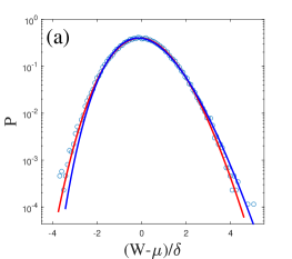
(a)

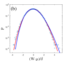
(b)

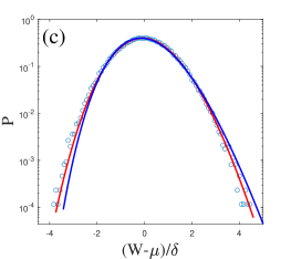
(c)

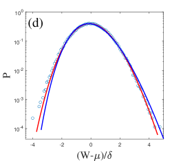
(d)

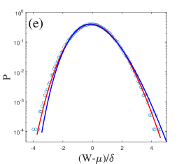
(e)

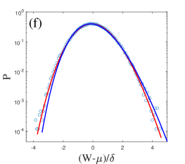
(f)

Figure 1: Probability distributions for $W(L,t)$ in the temporal correlated KPZ equation with different $\theta$: (a) $\theta=0.00$, (b) $\theta=0.10$, (c) $\theta=0.20$, (d) $\theta=0.25$, (e) $\theta=0.30$, (f) $\theta=0.40$. All data are averaged over $10^{5}$ independent realizations. Comparisons with TW-GSE (red solid line) and Tracy-Widom Gaussian orthogonal ensemble (TW-GOE) (blue solid line) are also provided correspondingly.

(a)

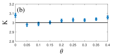
(b)

Figure 2: The estimated values of (a) skewness $S$ and (b) kurtosis $K$ with error bars for probability distributions of $W$ for KPZ model with long-range temporal correlation. The Gaussian distribution values (solid lines) are provided for quantitative comparison.

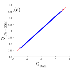
(a)

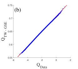
(b)

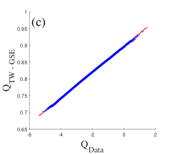
(c)

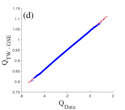
(d)

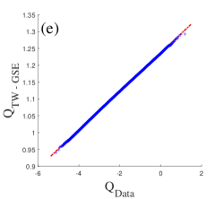
(e)

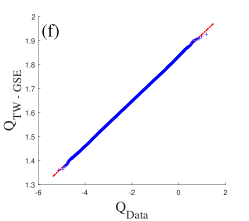
(f)

Figure 3: The Q-Q plots of TW-GSE versus simulation data for different $\theta$. The values of $\theta$ chosen here are same with Fig.1.

In this subsection, we investigate numerically the temporal correlated KPZ system in the (1+1)-dimensions based on LS numerical scheme. To study the effects of long-range temporal correlation on probability distribution for kinetic roughening within the early growth regimes, we calculate the time evolution of growth height and $W(L,t)$. Here, system size $L=4096$ and growth time $t=300$ are used. The distributions for $W(L,t)$ with different $\theta$ in the range [0, 0.40] are shown in Fig.1. Our results indicate that, when $\theta\geq 0$, every distribution is positive skewness, meanwhile, it has a longer tail in the right part, and fits highly the Tracy-Widom Gaussian symplectic ensemble (TW-GSE). It is evident that the long-range temporal correlation has a little effect for the probability distributions of $W(L,t)$.

Figure 2 shows $S$ and $K$ with error bars of $W(L,t)$ for different $\theta$. We find that both $S$ and $K$ have a similar trend. With increasing $\theta$ from zero, $S$ and $K$ suddenly decline and then gradually increase with an obvious trend, which also implies that the effect of long-range temporal correlation on the distribution of $W$ really exists. To compare TW distributions with simulation data from another point, we adopt a quantile-quantile (Q-Q) plot , a method to determine intuitively whether two series of numbers obey the same distribution, to analyze simulation data mentioned above. The corresponding results of the Q-Q plot are shown in Fig.3. Through quantitative comparison of TW-GSE (${{\rm{Q}}_{TW-GSE}}$) with simulation data (${{\rm{Q}}_{Data}}$), we find that distributions of $W(L,t)$ generally obey TW-GSE. Thus, these results show that long-range temporally correlated noise not obviously changes the distribution form of $W(L,t)$ for this kind of correlated KPZ growth.

3.2 The KPZ equation with long-range spatial correlation

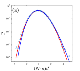
(a)

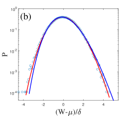
(b)

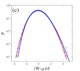
(c)

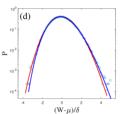
(d)

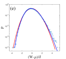
(e)

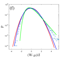
(f)

Figure 4: Probability distributions for $W(L,t)$ in the spatial correlated KPZ system with different $\rho$: (a) $\rho=0.00$, (b) $\rho=0.10$, (c) $\rho=0.20$, (d) $\rho=0.25$, (e) $\rho=0.30$, (f) $\rho=0.40$. All data are averaged over $10^{5}$ independent realizations. The suitable distributions are provided for comparison: TW-GSE (red solid line), TW-GOE (blue solid line) and Gumbel distribution (green solid line).

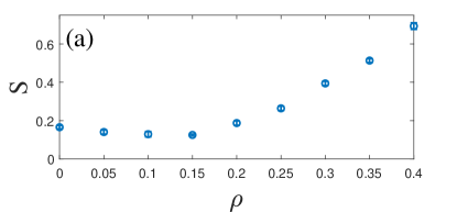
(a)

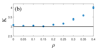
(b)

Figure 5: The estimated values of (a) skewness $S$ and (b) kurtosis $K$ with error bars for probability distributions for $W(L,t)$ with different $\rho$, which compare quantitatively with the Gaussian (solid lines).

To investigate probability distributions for interface width of the spatial correlated KPZ system within the early growth regimes, we perform numerical simulations with different spatial correlation exponent $\rho$. System size $L=4096$ and growth time $t=300$ are used, and numerical results are presented in Fig.4. We find that the distributions of $W(L,t)$ quantitatively fit TW-GSE when $\rho\leq 0.15$, and with $\rho$ increasing, transfer tend to the Gumbel distribution. In particular, the distribution is similar to the Tracy-Widom Gaussian orthogonal ensemble (TW-GOE) for $0.20<\rho\leq 0.30$.

Furthermore, we also analyze the variations of $S$ and $K$ with different $\rho$, the corresponding results are shown in Figs.5(a) and 5(b), respectively. We find that, as $\rho$ increases, $S$ and $K$ have similar changing trends. More specifically, both $S$ and $K$ vary very slowly with $\rho$ increasing, and all approach to the values of TW-GSE for $\rho\leq 0.15$, which indicates that the distribution form is not significantly affected by long-range spatially correlated noise. When $\rho>0.15$, $S$ and $K$ appear to increase with $\rho$, the distribution becomes more right-skewed, and has more fat tail. These results show that long-range spatial correlation could affect gradually the distribution form of $W(L,t)$ within this correlated regime. These characteristics are also consistent with our numerical results, as shown in Fig.4.

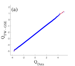
(a)

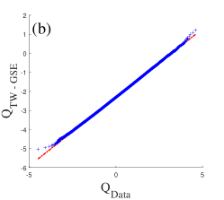
(b)

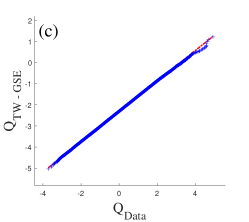
(c)

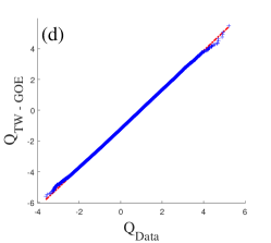
(d)

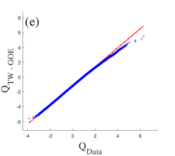
(e)

(f)

Figure 6: The Q-Q plots of TW-GSE, TW-GOE versus simulation data for different $\rho$. The values of $\rho$ chosen here are same with Fig.4.

We also analyze simulation data using the Q-Q plot method, and these plots for different $\rho$ show similar results with the predictions mentioned above, as shown in Fig.6. According to a comparison of the quantile of fitting distribution and simulation data, there exists an evident discrepancy in the Q-Q plot for $\rho>0.30$, which implies that simulation data are not completely in agreement with the TW-GOE. As $\rho$ increases, the distribution becomes more asymmetric, leptokurtic, and fat-tailed, and tends to an unknown distribution. Thus, it is not very clear that which forms obey when $\rho>0.30$. Interestingly, the distribution of $W(L,t)$ with the strong spatial correlation has a trend that approaches to the Gumbel form. Meanwhile, we also find the distribution form of $W^{2}(L,t)$ within the large spatial correlated regimes perfectly fits Gumbel distribution.

4 Conclusions

In summary, we have performed extensive numerical investigations in the (1+1)-dimensional KPZ system with long-range temporally and spatially correlated noises. Our results show that long-range temporal and spatial correlations could affect probability distributions of $W(L,t)$ to a certain extent, and the nontrivial effects of long-range temporal and spatial correlations are obviously different. For the temporal correlated KPZ equation, probability distributions of $W(L,t)$ have little effect by temporally correlated noise and are in quantitative agreement with TW-GSE distribution as $\rho$ increases. And Q-Q plots further confirm the results, and the variations of $S$ and $K$ also find that distribution form have small change with $\theta$ increasing. For the spatial correlated KPZ system, we find that distribution forms of $W(L,t)$ are not significantly affected by long-range spatially correlated noise for $\rho\leq 0.15$, which still belongs to TW-GSE based on several independent estimation methods. When $\rho\geq 0.15$, distribution form evidently depends on $\rho$. And variations of $S$ and $K$ with $\rho$ also show a strong and positive dependence for this correlated regime. Moreover, the distributions become more skew and thin with $\rho$ increasing. Finally, the distribution of $W(L,t)$ is quantitatively similar to that of Gumbel distribution, which implies that the spatial correlate KPZ equation smoothly tends to another universality class when $\rho$ increases gradually. However, it is still unclear what type of distribution form for the spatial correlated KPZ system when $\rho$ is beyond a certain critical threshold.

Acknowledgments

We would like to thank Yueheng Lan for useful discussions and kind help. This work is supported by Key Academic Discipline Project of China University of Mining and Technology under Grant No. 2022WLXK04.

Funding

H. X. is supported by Key Academic Discipline Project of China University of Mining and Technology under Grant No. 2022WLXK04.

Data Availability

The datasets generated during and/or analysed during the current study are available from the corresponding author (Hui Xia) on reasonable request.

Conflict of interest

The authors declare no conflict of interest.

References

- \bibcommenthead
- (1) Barabási, A.-L., Stanley, H.E.: Fractal Concepts in Surface Growth. Cambridge University Press, Cambridge, England (1995)
- (2) Chen, L., Lee, C.F., Toner, J.: Mapping two-dimensional polar active fluids to two-dimensional soap and one-dimensional sandblasting. Nature Communications 7(1), 1–10 (2016). https://doi.org/10.1038/ncomms12215
- (3) Veynante, D., Vervisch, L.: Turbulent combustion modeling. Progress in Energy and Combustion Science 28(3), 193–266 (2002). https://doi.org/10.1016/S0360-1285(01)00017-X
- (4) Kardar, M., Parisi, G., Zhang, Y.-C.: Dynamic scaling of growing interfaces. Phys. Rev. Lett. 56, 889–892 (1986). https://doi.org/10.1103/PhysRevLett.56.889
- (5) Family, F., Vicsek, T.: Scaling of the active zone in the Eden process on percolation networks and the ballistic deposition model. Journal of Physics A: Mathematical and General 18(2), 75–81 (1985). https://doi.org/10.1088/0305-4470/18/2/005
- (6) Chu, S., Kardar, M.: Probability distributions for directed polymers in random media with correlated noise. Phys. Rev. E 94, 010101 (2016). https://doi.org/10.1103/PhysRevE.94.010101
- (7) Halpin-Healy, T., Zhang, Y.-C.: Kinetic roughening phenomena, stochastic growth, directed polymers and all that. Aspects of multidisciplinary statistical mechanics. Physics Reports 254(4), 215–414 (1995). https://doi.org/10.1016/0370-1573(94)00087-J
- (8) Squizzato, D., Canet, L., Minguzzi, A.: Kardar-Parisi-Zhang universality in the phase distributions of one-dimensional exciton-polaritons. Phys. Rev. B 97, 195453 (2018). https://doi.org/10.1103/PhysRevB.97.195453
- (9) Kulkarni, M., Lamacraft, A.: Finite-temperature dynamical structure factor of the one-dimensional Bose gas: From the Gross-Pitaevskii equation to the Kardar-Parisi-Zhang universality class of dynamical critical phenomena. Phys. Rev. A 88, 021603 (2013). https://doi.org/10.1103/PhysRevA.88.021603
- (10) Gladilin, V.N., Ji, K., Wouters, M.: Spatial coherence of weakly interacting one-dimensional nonequilibrium bosonic quantum fluids. Phys. Rev. A 90, 023615 (2014). https://doi.org/10.1103/PhysRevA.90.023615
- (11) Altman, E., Sieberer, L.M., Chen, L., Diehl, S., Toner, J.: Two-dimensional superfluidity of exciton polaritons requires strong anisotropy. Phys. Rev. X 5, 011017 (2015). https://doi.org/10.1103/PhysRevX.5.011017
- (12) Mathey, S., Gasenzer, T., Pawlowski, J.M.: Anomalous scaling at nonthermal fixed points of Burgers’ and Gross-Pitaevskii turbulence. Phys. Rev. A 92, 023635 (2015). https://doi.org/10.1103/PhysRevA.92.023635
- (13) Zhang, Y.-C.: Replica scaling analysis of interfaces in random media. Phys. Rev. B 42, 4897–4900 (1990). https://doi.org/10.1103/PhysRevB.42.4897
- (14) Hentschel, H.G.E., Family, F.: Scaling in open dissipative systems. Phys. Rev. Lett. 66, 1982–1985 (1991). https://doi.org/10.1103/PhysRevLett.66.1982
- (15) Hanfei, Ma, B.: Scaling analysis of Langevin-type equations. Phys. Rev. E 47, 3738–3740 (1993). https://doi.org/10.1103/PhysRevE.47.3738
- (16) Prähofer, M., Spohn, H.: Universal distributions for growth processes in dimensions and random matrices. Phys. Rev. Lett. 84, 4882–4885 (2000). https://doi.org/10.1103/PhysRevLett.84.4882
- (17) Sasamoto, T., Spohn, H.: One-dimensional Kardar-Parisi-Zhang equation: An exact solution and its universality. Phys. Rev. Lett. 104, 230602 (2010). https://doi.org/10.1103/PhysRevLett.104.230602
- (18) Halpin-Healy, T.: ()-dimensional directed polymer in a random medium: Scaling phenomena and universal distributions. Phys. Rev. Lett. 109, 170602 (2012). https://doi.org/10.1103/PhysRevLett.109.170602
- (19) Medina, E., Hwa, T., Kardar, M., Zhang, Y.-C.: Burgers equation with correlated noise: Renormalization-group analysis and applications to directed polymers and interface growth. Phys. Rev. A 39, 3053–3075 (1989). https://doi.org/10.1103/PhysRevA.39.3053
- (20) Katzav, E., Schwartz, M.: Self-consistent expansion for the Kardar-Parisi-Zhang equation with correlated noise. Phys. Rev. E 60, 5677–5680 (1999). https://doi.org/10.1103/PhysRevE.60.5677
- (21) Katzav, E., Schwartz, M.: Kardar-Parisi-Zhang equation with temporally correlated noise: A self-consistent approach. Phys. Rev. E 70, 011601 (2004). https://doi.org/10.1103/PhysRevE.70.011601
- (22) Song, T., Xia, H.: Extensive numerical simulations of surface growth with temporally correlated noise. Phys. Rev. E 103, 012121 (2021). https://doi.org/10.1103/PhysRevE.103.012121
- (23) Meakin, P., Jullien, R.: Spatially correlated Ballistic Deposition. Europhysics Letters (EPL) 9(1), 71–76 (1989). https://doi.org/10.1209/0295-5075/9/1/013
- (24) Meakin, P., Jullien, R.: Spatially correlated ballistic deposition on one- and two-dimensional surfaces. Phys. Rev. A 41, 983–993 (1990). https://doi.org/10.1103/PhysRevA.41.983
- (25) Amar, J.G., Lam, P.-M., Family, F.: Surface growth with long-range correlated noise. Phys. Rev. A 43, 4548–4550 (1991). https://doi.org/10.1103/PhysRevA.43.4548
- (26) Peng, C.-K., Havlin, S., Schwartz, M., Stanley, H.E.: Directed-polymer and ballistic-deposition growth with correlated noise. Phys. Rev. A 44, 2239–2242 (1991). https://doi.org/10.1103/PhysRevA.44.R2239
- (27) Pang, N.-N., Yu, Y.-K., Halpin-Healy, T.: Interfacial kinetic roughening with correlated noise. Phys. Rev. E 52, 3224–3227 (1995). https://doi.org/10.1103/PhysRevE.52.3224
- (28) Mukherji, S., Bhattacharjee, S.M.: Nonlocality in kinetic roughening. Phys. Rev. Lett. 79, 2502–2505 (1997). https://doi.org/10.1103/PhysRevLett.79.2502
- (29) Li, M.S.: Surface growth with spatially correlated noise. Phys. Rev. E 55, 1178–1180 (1997). https://doi.org/10.1103/PhysRevE.55.1178
- (30) Chattopadhyay, A.K., Bhattacharjee, J.K.: Self-consistent mode coupling and the Kardar-Parisi-Zhang equation with spatially correlated noise. Europhysics Letters (EPL) 42(2), 119–124 (1998). https://doi.org/10.1209/epl/i1998-00211-3
- (31) Frey, E., Täuber, U.C., Janssen, H.K.: Scaling regimes and critical dimensions in the Kardar-Parisi-Zhang problem. Europhysics Letters (EPL) 47(1), 14–20 (1999). https://doi.org/10.1209/epl/i1999-00343-4
- (32) Verma, M.K.: Intermittency exponents and energy spectrum of the Burgers and KPZ equations with correlated noise. Physica A: Statistical Mechanics and its Applications 277(3), 359–388 (2000). https://doi.org/10.1016/S0378-4371(99)00544-0
- (33) Katzav, E.: Self-consistent expansion results for the nonlocal Kardar-Parisi-Zhang equation. Phys. Rev. E 68, 046113 (2003). https://doi.org/10.1103/PhysRevE.68.046113
- (34) Katzav, E.: Effect of long range interactions on the growth of compact clusters under deposition. The European Physical Journal B 54(2), 137–140 (2006). https://doi.org/10.1140/epjb/e2006-00437-9
- (35) Katzav, E.: Fixing the fixed-point system—applying dynamic renormalization group to systems with long-range interactions. Physica A: Statistical Mechanics and its Applications 392(8), 1750–1755 (2013). https://doi.org/10.1016/j.physa.2013.01.010
- (36) Kloss, T., Canet, L., Delamotte, B., Wschebor, N.: Kardar-Parisi-Zhang equation with spatially correlated noise: A unified picture from nonperturbative renormalization group. Phys. Rev. E 89, 022108 (2014). https://doi.org/10.1103/PhysRevE.89.022108
- (37) Morais, P.A., Oliveira, E.A., Araújo, N.A.M., Herrmann, H.J., Andrade, J.S.: Fractality of eroded coastlines of correlated landscapes. Phys. Rev. E 84, 016102 (2011). https://doi.org/10.1103/PhysRevE.84.016102
- (38) Xia, H., Tang, G., Lan, Y.: Numerical analysis of long-range spatial correlations in surface growth. Phys. Rev. E 94, 062121 (2016). https://doi.org/10.1103/PhysRevE.94.062121
- (39) Niggemann, O., Hinrichsen, H.: Sinc noise for the Kardar-Parisi-Zhang equation. Phys. Rev. E 97, 062125 (2018). https://doi.org/10.1103/PhysRevE.97.062125
- (40) Fedorenko, A.A.: Elastic systems with correlated disorder: Response to tilt and application to surface growth. Phys. Rev. B 77, 094203 (2008). https://doi.org/10.1103/PhysRevB.77.094203
- (41) Lam, C.-H., Sander, L.M., Wolf, D.E.: Surface growth with temporally correlated noise. Phys. Rev. A 46, 6128–6131 (1992). https://doi.org/10.1103/PhysRevA.46.R6128
- (42) Strack, P.: Dynamic criticality far from equilibrium: One-loop flow of Burgers-Kardar-Parisi-Zhang systems with broken Galilean invariance. Phys. Rev. E 91, 032131 (2015). https://doi.org/10.1103/PhysRevE.91.032131
- (43) Song, T., Xia, H.: Long-range temporal correlations in the Kardar–Parisi–Zhang growth: numerical simulations. Journal of Statistical Mechanics: Theory and Experiment 2016(11), 113206 (2016). https://doi.org/10.1088/1742-5468/2016/11/113206
- (44) Squizzato, D., Canet, L.: Kardar-Parisi-Zhang equation with temporally correlated noise: A nonperturbative renormalization group approach. Phys. Rev. E 100, 062143 (2019). https://doi.org/%****␣sn-article.bbl␣Line␣700␣****10.1103/PhysRevE.100.062143
- (45) Alés, A., López, J.M.: Faceted patterns and anomalous surface roughening driven by long-range temporally correlated noise. Phys. Rev. E 99, 062139 (2019). https://doi.org/10.1103/PhysRevE.99.062139
- (46) Foltin, G., Oerding, K., Rácz, Z., Workman, R.L., Zia, R.K.P.: Width distribution for random-walk interfaces. Phys. Rev. E 50, 639–642 (1994). https://doi.org/10.1103/PhysRevE.50.R639
- (47) Rácz, Z., Plischke, M.: Width distribution for (2+1)-dimensional growth and deposition processes. Phys. Rev. E 50, 3530–3537 (1994). https://doi.org/10.1103/PhysRevE.50.3530
- (48) Antal, T., Rácz, Z.: Dynamic scaling of the width distribution in Edwards-Wilkinson type models of interface dynamics. Phys. Rev. E 54, 2256–2260 (1996). https://doi.org/10.1103/PhysRevE.54.2256
- (49) Marinari, E., Pagnani, A., Parisi, G., Rácz, Z.: Width distributions and the upper critical dimension of Kardar-Parisi-Zhang interfaces. Phys. Rev. E 65, 026136 (2002). https://doi.org/10.1103/PhysRevE.65.026136
- (50) Aarão Reis, F.D.A.: Numerical study of roughness distributions in nonlinear models of interface growth. Phys. Rev. E 72, 032601 (2005). https://doi.org/10.1103/PhysRevE.72.032601
- (51) Mandelbrot, B.B.: A fast fractional gaussian noise generator. Water Resources Research 7(3), 543–553 (1971). https://doi.org/10.1029/WR007i003p00543
- (52) Moser, K., Kertész, J., Wolf, D.E.: Numerical solution of the Kardar-Parisi-Zhang equation in one, two and three dimensions. Physica A: Statistical Mechanics and its Applications 178(2), 215–226 (1991). https://doi.org/10.1016/0378-4371(91)90017-7
- (53) Dasgupta, C., Kim, J.M., Dutta, M., Das Sarma, S.: Instability, intermittency, and multiscaling in discrete growth models of kinetic roughening. Phys. Rev. E 55, 2235–2254 (1997). https://doi.org/10.1103/PhysRevE.55.2235
- (54) Miranda, V.G., Aarão Reis, F.D.A.: Numerical study of the Kardar-Parisi-Zhang equation. Phys. Rev. E 77, 031134 (2008). https://doi.org/10.1103/PhysRevE.77.031134
- (55) Gallego, R., Castro, M., López, J.M.: On the origin of multiscaling in stochastic-field models of surface growth. The European Physical Journal B 89(9), 1–7 (2016). https://doi.org/10.1140/epjb/e2016-70132-5
- (56) Li, B., Tan, Z., Jiao, Y., Xia, H.: Universality in a class of the modified Villain–Lai–Das Sarma equation. Journal of Statistical Mechanics: Theory and Experiment 2021(2), 023210 (2021). https://doi.org/10.1088/1742-5468/abdd16
- (57) Lam, C.-H., Shin, F.G.: Improved discretization of the Kardar-Parisi-Zhang equation. Phys. Rev. E 58, 5592–5595 (1998). https://doi.org/%****␣sn-article.bbl␣Line␣900␣****10.1103/PhysRevE.58.5592