Last-Iterate Convergence of Optimistic Gradient Method for Monotone Variational Inequalities

Abstract

The Past Extragradient (PEG) [Popov, 1980] method, also known as the Optimistic Gradient method, has known a recent gain in interest in the optimization community with the emergence of variational inequality formulations for machine learning. Recently, in the unconstrained case, Golowich et al. [2020a] proved that a ${\cal O}(\nicefrac{{1}}{{N}})$ last-iterate convergence rate in terms of the squared norm of the operator can be achieved for Lipschitz and monotone operators with a Lipschitz Jacobian. In this work, by introducing a novel analysis through potential functions, we show that (i) this ${\cal O}(\nicefrac{{1}}{{N}})$ last-iterate convergence can be achieved without any assumption on the Jacobian of the operator, and (ii) it can be extended to the constrained case, which was not derived before even under Lipschitzness of the Jacobian. The proof is significantly different from the one known from Golowich et al. [2020a], and its discovery was computer-aided. Those results close the open question of the last iterate convergence of PEG for monotone variational inequalities.

1 Introduction

Minimax optimization, and more generally variational inequality problems, has known a surge of interest with the recent introduction of machine learning formulation with multiple objectives such as robust optimization [Ben-Tal et al., 2009], control [Hast et al., 2013], generative adversarial networks (GANs) [Goodfellow et al., 2014], and adversarial training [Goodfellow et al., 2015, Madry et al., 2018]. In this work, given a convex set $\mathcal{X}$, we focus on solving monotone variational inequalities:

$$\text{find }x^{*}\in{\cal X}\quad\text{such that}\quad\langle F(x^{*}),x-x^{*}\rangle\geq 0\,,\quad\forall x\in\mathcal{X}\subseteq\mathbb{R}^{d}.$$ (VIP-C)

In the unconstrained case ($\mathcal{X}=\mathbb{R}^{d}$,) this optimality condition can be simplified as

$$\text{find }x^{*}\in\mathbb{R}^{d}\quad\text{such that}\quad F(x^{*})=0.$$ (VIP-U)

We focus on the monotone and Lipschitz setting which is sufficient to ensure the existence of solutions for VIP-C and is the standard setting to study first-order methods [Facchinei and Pang, 2003].

Assumption 1.

$F:{\cal X}\to\mathbb{R}^{d}$ is monotone and $L$-Lipschitz, i.e., for all $x,y\in{\cal X}$

$$\langle F(x)-F(y),x-y\rangle\geq 0\qquad\text{and}\qquad\|F(x)-F(y)\|\leq L\|x-y\|,$$ (1)

furthermore, there exists some $x^{*}\in{\cal X}$ which is a solution to (VIP-C).

In this context, it is well known that the standard Gradient method $x^{k+1}=\mathop{\mathrm{proj}}\nolimits[x^{k}-\gamma F(x^{k})]$ (also known as the Forward method), where $\mathop{\mathrm{proj}}\nolimits(x):=\mathop{\arg\!\min}_{y\in\mathcal{X}}\|y-x\|^{2}$, does not always converge. Two important first-order methods have been introduced to circumvent this issue: the extragradient method (EG) [Korpelevich, 1976]

$$\widetilde{x}^{k}=\mathop{\mathrm{proj}}\nolimits[x^{k}-\gamma F(x^{k})],\quad x^{k+1}=\mathop{\mathrm{proj}}\nolimits[x^{k}-\gamma F(\widetilde{x}^{k})],\quad\text{for all}\;k>0\,,$$ (Proj-EG)

and the past extragradient method (PEG) [Popov, 1980] defined via the following recursions: $\widetilde{x}^{0}=x^{0}\in{\cal X}$, $x^{1}=\mathop{\mathrm{proj}}\nolimits[x^{0}-\gamma F(x^{0})]$, and

$$\widetilde{x}^{k}=\mathop{\mathrm{proj}}\nolimits[x^{k}-\gamma F(\widetilde{x}^{k-1})],\quad x^{k+1}=\mathop{\mathrm{proj}}\nolimits[x^{k}-\gamma F(\widetilde{x}^{k})]\,,\quad\text{for all}\;k>0\,.$$ (Proj-PEG)

In the unconstrained case, the method simplifies to $x^{1}=x^{0}-\gamma F(x^{0})$, and for all $k\geq 0$

$$\widetilde{x}^{k}=x^{k}-\gamma F(\widetilde{x}^{k-1}),\quad x^{k+1}=x^{k}-\gamma F(\widetilde{x}^{k})\,.$$ (PEG)

with the convention that $F(\widetilde{x}^{-1})=0$, allowing us to use the above recursions for $k=0$. Note that, in this case, PEG is often studied in the equivalent form called Optimistic Gradient Method (OG):

$$\widetilde{x}^{k+1}=\widetilde{x}^{k}-2\gamma F(\widetilde{x}^{k})+\gamma F(\widetilde{x}^{k-1})\,.$$ (OG)

Under Assumption 1, some recent works have managed to leverage tools for computer-aided proofs to show a ${\cal O}(\nicefrac{{1}}{{N}})$ (for the squared norm of the operator/squared residual) last-iterate convergence rate for the extragradient method (EG), where $N$ denotes the total number of iterations. This was achieved in the unconstrained case by [Gorbunov et al., 2021] via the performance estimation technique [Drori and Teboulle, 2014, Taylor et al., 2017c] and in the constrained case [Cai et al., 2022] via Sum-of-Squares (SOS) techniques [Shor, 1987, Nesterov, 2000, Parrilo, 2000, Lasserre, 2001] (note that “performance estimation” corresponds to SOS of order $2$). Our work leverages performance estimation problems (PEPs) for obtaining similar convergence results for PEG and Proj-PEG.

Outline.

This paper is composed of five sections. In §1 we introduce our motivations, our main results and discuss the related work. In §2, we show how we used PEP to hint us toward a valid potential function. We prove the convergence of PEG in the unconstrained case and the constrained cases respectively in §3 and §4. Finally, we discuss our results and future research directions in §5. Since the proof in the unconstrained case is slightly simpler than in the constrained one (although it cannot be straightforwardly deduced from our analysis in the constrained case), in the main part of the paper, we discuss in detail the way to the proof in the unconstrained case, and defer the proofs and other details on the constrained case to Appendices C and D. Codes for verifying the potentials and convergence rates are publicly available: https://github.com/eduardgorbunov/potentials_and_last_iter_convergence_for_VIPs, the codes rely on the PEP packages [Taylor et al., 2017b, Goujaud et al., 2022] as well as on YALMIP [Lofberg, 2004].

1.1 Presentation of Our Main Results

For variational inequalities with possibly unbounded domains, there exist two main standard convergence criteria in the literature. The first one is the restricted gap function [Nesterov, 2007]

$$\texttt{Gap}_{F,R}(x^{k})=\max\limits_{y\in\mathcal{X}:\|y-x^{*}\|\leq R}\langle F(y),x^{k}-y\rangle,$$ (2)

where $x^{*}$ is any solution of VIP-C. This quantity is an actual gap function only if $\|x^{k}-x^{*}\|\leq R$ and that it cannot be extended to the non-monotone setting where, for instance, there might exist several points where $F(x)=0$. Since we show that $\|x^{k}-x^{*}\|\leq\tfrac{\sqrt{41}}{3}\|x^{0}-x^{*}\|$ and $\|x^{k}-x^{*}\|\leq\sqrt{2}\|x^{0}-x^{*}\|+\tfrac{\sqrt{2}}{L}\|F(x^{0})\|,\,\forall k\geq 0$ in the unconstrained and constrained cases respectively, we can set $R=\tfrac{\sqrt{41}}{3}\|x^{0}-x^{*}\|$ in the unconstrained case and $R=\sqrt{3}\|x^{0}-x^{*}\|+\tfrac{1}{\sqrt{30}L}\|F(x^{0})\|,$ in the constrained case and have that $\texttt{Gap}_{F}(x^{k}):=\texttt{Gap}_{F,R}(x^{k})$ is a gap function for all $k\geq 0$. Another convergence criterion is the (squared) norm of the residual $\|x^{k+1}-x^{k}\|^{2}$. In the unconstrained setting, it is proportional to the (squared) norm of the operator $\|F(\widetilde{x}^{k})\|^{2}$. This criterion is also valid as a local convergence certificate in the non-monotone case. We believe this criterion depicts a more precise picture than the standard gap function since it does not require to use a bound on $\|x^{k}-x^{*}\|$ to be valid and it generalizes to non-monotone settings. Nevertheless, we provide convergence results in terms of both criteria.

Our main theorems introduce new potential/Lyapunov functions for PEG with two main consequences: (i) it implies a uniform bound on $\|x^{N}-x^{*}\|$, and (ii) we show a ${\cal O}(\nicefrac{{1}}{{\sqrt{N}}})$ convergence rate for $\|F(x^{N})\|$ and $\texttt{Gap}_{F}(x^{N})$ in the unconstrained case and for $\|x^{N}-x^{N-1}\|$ and $\texttt{Gap}_{F}(x^{N})$ in the constrained case. Theorem 1 and Theorem 2 below provide simplified versions of the results; more detailed/general statements are presented later in §3 and §4.

Theorem 1 (Unconstrained Case).

Under Assumption 1, for all $N\geq 0$ and $\gamma=\nicefrac{{1}}{{3L}}$, we have

$$\|F(x^{N})\|^{2}\leq\frac{123L^{2}\|x^{0}-x^{*}\|^{2}}{N+32},\quad\texttt{Gap}_{F}(x^{N})\leq\frac{125L\|x^{0}-x^{*}\|^{2}}{\sqrt{3N+96}},$$ (3)

where $x^{*}$ is any solution to VIP-U.

Theorem 2 (Constrained Case).

Under Assumption 1, for all $N\geq 2$ the iterates of Proj-PEG with $\gamma=\nicefrac{{1}}{{4L}}$ satisfy

$$\|x^{N}-x^{N-1}\|^{2}\leq\frac{24H_{0}^{2}}{3N+32},\quad\texttt{Gap}_{F}(x^{N})\leq\frac{32L\sqrt{3}H_{0}^{2}}{\sqrt{3N+32}},$$ (4)

where $H_{0}>0$ is such that $H_{0}^{2}=3\|x^{0}-x^{*}\|^{2}+\tfrac{1}{30L^{2}}\|F(x^{0})\|^{2}$ and $x^{*}$ is any solution to VIP-C.

1.2 Related Work

Linear last-iterate convergence rates.

Motivated by nonconvex-nonconcave minimax formulation such as GANs, last-iterate convergences in the context of variational inequalities is the focus of many recent works. Linear convergence rates have been obtained, in the bilinear setting, the (local) strongly monotone setting, and similar settings such as sufficient bilinearity [Tseng, 1995, Daskalakis et al., 2018, Liang and Stokes, 2019, Gidel et al., 2019a, b, Mokhtari et al., 2019, Peng et al., 2020, Zhang and Yu, 2020, Abernethy et al., 2019, Loizou et al., 2020, Hsieh et al., 2019, Azizian et al., 2020a, b].

Sublinear last-iterate convergence rates for EG and PEG.

More recently, the community has been focusing on the question of last-iterate convergence rate in the monotone setting (i.e., without strong monotonicity or sufficient bilinearity). For monotone and Lipschtiz operators obtaining ${\cal O}(\nicefrac{{1}}{{N}})$ last-iterate convergence rate of PEG was explicitly stated as an open question in [Hsieh et al., 2019]. In the unconstrained case, Golowich et al. [2020a] achieve this result by adding an assumption on the Jacobian of $F$ being Lipschitz. For EG as similar result has been obtained in Golowich et al. [2020b]. Eventually, a last-iterate convergence rate for EG has been provided by Gorbunov et al. [2021] in the unconstrained case and by Cai et al. [2022] in the constrained case, both under Assumption 1 solely. The question of last-iterate convergence rate for PEG both in the unconstrained and constrained cases mentioned by Hsieh et al. [2019] remained open until now and is the central question addressed here.

Variants of EG and PEG.

Recently, some modification of EG with anchoring (a.k.a., Halpern iteration [Halpern, 1967]) enjoying (accelerated) last-iterate convergence rates have been proposed by [Yoon and Ryu, 2021], [Lee and Kim, 2021], and [Diakonikolas, 2020]. This work is concerned with method achieving the suboptimal ${\cal O}(\nicefrac{{1}}{{N}})$ rate, whereas ${\cal O}(\nicefrac{{1}}{{N^{2}}})$ can be achieved using optimal methods [Diakonikolas, 2020, Yoon and Ryu, 2021, Lee and Kim, 2021, Tran-Dinh and Luo, 2021, Tran-Dinh, 2022]. We argue that (i) PEG is still largely used in practice, (ii) PEG is simple and more flexible, and (iii) that it benefits from additional advantageous properties, such as adaptivity to additional problem structure. Regarding (i) we would like to mention that Daskalakis et al. [2018] show that PEG-based algorithms (like PEG-Adam) perform well in training WGAN on CIFAR10 and PEG/OG have been extensively used in regret matching [Brown and Sandholm, 2019], counterfactual regret minimization [Farina et al., 2019], and for training agents to play poker [Anagnostides et al., 2022]. With a bit more details about (ii) and (iii): PEG is highly flexible and can be applied to online learning [Golowich et al., 2020a] or to the non-monotone variational inequalities [Daskalakis et al., 2018]. In contrast, EG with anchoring (EAG) [Yoon and Ryu, 2021]

$$\widetilde{x}^{k}=x^{k}+\beta_{k}\left(x^{0}-x^{k}\right)-\gamma F(x^{k}),\quad x^{k+1}=x^{k}+\beta_{k}\left(x^{0}-x^{k}\right)-\gamma F(x^{k}),$$ (EAG)

where $\beta_{k}\in[0,1)$ is the anchoring coefficient, cannot be applied to online learning easily (EG/EAG are not no-regret [Golowich et al., 2020a]) and may not be desirable in the non-monotone setting since it may make some “bad” stationary points attractive.

Example 1.1.

Let us consider a single example classification task with a deep linear neural network $\min_{w\in\mathbb{R}^{3}}(y-w_{3}w_{2}w_{1}x)^{2}:=f(w)$. It has a undesirable stationary point $w^{s}=(0,0,0)$. Because $\nabla^{2}f(w^{s})=0$, for an initialization $w^{0}$ close enough to $w^{s}$ and any small enough stepsize, EAG will converge to $w^{s}$ while PEG and EG will not, except for a zero measure set of initializations.

A further practical reason that renders “simple” methods (such as PEG and EG) attractive is that simple methods are typically adaptive to additional problem structure (better behavior than predicted by the analysis when the problem has beneficial additional properties). As an example, PEG converges sublinearly for monotone operator (this is the topic of this work) and linearly for strongly-monotone operators [Gidel et al., 2019a] under the same stepsize rules. This stands in sharp contrast with optimal methods, which require to be tuned to the specific setting at hand (and in particular, which require the knowledge of the setting at hand).

2 A Path to the Proof

In this section, we show a direct approach for assessing the worst-case convergence rate of the last iterate of PEG. The Lyapunov analyses provided in the next sections are grounded on the numerical results presented here. Whereas converting those numerical results into a Lyapunov analysis is not direct, we believe that the material offers the comfortable privilege of a first clear ${\cal O}(\nicefrac{{1}}{{N}})$ baseline for the further convergence results, as well as a convenient approach for verifying Lyapunov functions.

Verifying ${\cal O}(\nicefrac{{1}}{{N}})$ last-iterate convergence rate.

This section contains our heuristic argument for concluding a ${\cal O}(\nicefrac{{1}}{{N}})$ convergence of $\|F(x^{N})\|^{2}$ for all $F$ satisfying our assumptions. This ingredient was the main motivation behind the investigations of the next sections. In short, our goal is to characterize the worst-case behavior of $\frac{\|F(x^{N})\|^{2}}{\|x^{0}-x^{*}\|^{2}}$ as a function of $N$ when $x^{N}$ is obtained from PEG. For doing that, we rely on the so-called performance estimation framework—first introduced in [Drori and Teboulle, 2014]. That is, we consider the problem of computing the worst-case value of $\frac{\|F(x^{N})\|^{2}}{\|x^{0}-x^{*}\|^{2}}$ (i.e., the worst possible $L$-Lipschitz and monotone $F$, worst dimension $d\in\mathbb{N}$, worst sequence of iterates $x^{0},\ldots,x^{N},\tilde{x}^{0},\ldots,\tilde{x}^{N-1}\in\mathbb{R}^{d}$ and worst solution $x^{*}\in\mathbb{R}^{d}$ to (VIP-U)):

$$G_{{\sf PEG}}(\gamma,L,N)= \max\limits_{\begin{subarray}{c}F,d,x^{*}\\ \tilde{x}^{0},\ldots,\tilde{x}^{N}\\ x^{0},\ldots,x^{N}\end{subarray}} \frac{\|F(x^{N})\|^{2}}{\|x^{0}-x^{*}\|^{2}}$$

s.t. $$F\text{ is monotone and $L$-Lipschitz,}$$

$$\tilde{x}^{0}=x^{0}\in\mathbb{R}^{d},x^{1}=x^{0}-\gamma F(x^{0})$$

$$\widetilde{x}^{k}=x^{k}-\gamma F(\widetilde{x}^{k-1}),\text{ for }k=1,\ldots,N,$$

$$x^{k+1}=x^{k}-\gamma F(\widetilde{x}^{k}),\text{ for }k=1,\ldots,N-1.$$

Such problems are often referred to as Performance Estimation Problems (PEPs). Whereas it is not clear how to solve this PEP (2), a few techniques from [Ryu et al., 2020, Taylor et al., 2017a] allow obtaining a semidefinite relaxation providing meaningful worst-case bounds. By solving those problems numerically, we are able to conjecture that $G_{{\sf PEG}}(\gamma,L,N)={\cal O}(\nicefrac{{1}}{{N}})$, as the convex relaxations provides upper bounds on $G_{{\sf PEG}}$ which appear to behave in ${\cal O}(\nicefrac{{1}}{{N}})$ in numerical experiments. More precisely, the convex relaxation under consideration arises from a sampled version of the previous problem (thereby passing from an infinite-dimensional problem to a finite-dimensional one). In other words, we consider a sampled version of $F$ with $g^{k}\approx F(x^{k})$ and $\widetilde{g}^{k}\approx F(\widetilde{x}^{k})$ (so the variables will be the iterates and the operators values at the iterates instead of the operator itself) and we require monotonicity and Lipschitzness to be satisfied at those points. For convenience, we define the set of samples $S=\{(x^{*},0)\}\cup\{(x^{k},g^{k})\}_{k=0}^{N}\cup\{(\widetilde{x}^{k},\widetilde{g}^{k})\}_{k=0}^{N}\subseteq\mathbb{R}^{d}\times\mathbb{R}^{d}$:

$$\widetilde{G}_{{\sf PEG}}(\gamma,L,N)= \max\limits_{\begin{subarray}{c}d\in\mathbb{N},x^{*}\in\mathbb{R}^{d}\\ \{(x^{k},g^{k})\}_{k=0}^{N}\subset\mathbb{R}^{d}\times\mathbb{R}^{d}\\ \{(\widetilde{x}^{k},\widetilde{g}^{k})\}_{k=0}^{N}\subseteq\mathbb{R}^{d}\times\mathbb{R}^{d}\end{subarray}} \|g^{N}\|^{2}$$ (6)

s.t. $$\langle g-h,x-y\rangle\geq 0\quad\forall(x,g),(y,h)\in S$$ (9)

$$\|g-h\|^{2}\leq L^{2}\|x-y\|^{2}\quad\forall(x,g),(y,h)\in S$$

$$\widetilde{x}^{0}=x^{0}\in\mathbb{R}^{d},x^{1}=x^{0}-\gamma g^{0}$$

$$\widetilde{x}^{k}=x^{k}-\gamma\widetilde{g}^{k-1},\text{ for }k=1,\ldots,N,$$

$$x^{k+1}=x^{k}-\gamma\widetilde{g}^{k},\text{ for }k=1,\ldots,N-1,$$

$$\|x^{0}-x^{*}\|^{2}\leq 1.$$

(Note that a classical homogeneity argument allows replacing the objective of (2) by $\|g^{N}\|^{2}$ plus the constraint $\|x^{0}-x^{*}\|^{2}\leq 1$; see, e.g., [Ryu et al., 2020, §3.1.1.].) In other words, we replace the constraint corresponding to the existence of monotone $L$-Lipschitz operator $F$ from (2) by the constraint that there exist sequences of points $\{x^{k}\}_{k=0}^{N},\{\widetilde{x}^{k}\}_{k=0}^{N}$ and $\{g^{k}\}_{k=0}^{N},\{\widetilde{g}^{k}\}_{k=0}^{N}$ such that they satisfy necessary conditions for the existence of monotone and $L$-Lipschitz operator $F$ interpolating them. Unfortunately, these constraints are not sufficient to ensure that there exists such monotone $L$-Lipschitz operator $F$ [Ryu et al., 2020]. That is, we can guarantee only that $\widetilde{G}_{{\sf PEG}}(\gamma,L,N)\geq G_{{\sf PEG}}(\gamma,L,N)$. Finallly, $\widetilde{G}_{{\sf PEG}}(\gamma,L,N)$ can be computed numerically using semidefinite programming (SDP) through standard solvers [Mosek, 2010, Sturm, 1999]. For formulating the computation of $\widetilde{G}_{{\sf PEG}}(\gamma,L,N)$ as an SDP we first substitute a number of variables: $\{x^{k}\}_{k=1}^{N}$ and $\{\widetilde{x}^{k}\}_{k=0}^{N}$ are linear combinations of $x^{0},\{g^{k}\}_{k=0}^{N},,\{\widetilde{g}^{k}\}_{k=1}^{N}$. Next, we notice that the objective and constraints of problem (6) are linear functions of all possible inner products of vectors from ${\bf V}\stackrel{{\scriptstyle\text{def}}}{{=}}(x^{*},x^{0},g^{0},\widetilde{g}^{1},g^{1},\widetilde{g}^{2},g^{2},\ldots,\widetilde{g}^{N},g^{N})$. That is, problem (6) is linear w.r.t. the elements of Gram matrix ${\bf G}={\bf V}^{\top}{\bf V}\succeq 0$ (we use the notation ${\bf G}\in\mathbb{S}_{+}^{2N+3}$ for denoting $(2N+3)\times(2N+3)$ symmetric positive semidefinite matrices). The problem also naturally features the constraint $\mathrm{rank}({\bf G})\leq 2N+3$, which becomes void due to maximization over the dimension $d$ in (6) (see, e.g., [Taylor et al., 2017c, Theorem 5]) and the $\widetilde{G}_{{\sf PEG}}(\gamma,L,N)$ can therefore be computed by solving a standard SDP:

$$\widetilde{G}_{{\sf PEG}}(\gamma,L,N)= \max\limits_{{\bf G}\in\mathbb{S}_{+}^{2N+3}} \mathrm{Tr}({\bf M}_{0}{\bf G})$$

s.t. $$\mathrm{Tr}({\bf M}_{i}{\bf G})\leq 0\text{ for }i=1,2,\ldots,2N(2N+1)+1,$$

$$\mathrm{Tr}({\bf M}_{-1}{\bf G})\leq 1,$$

where $\{{\bf M}_{i}\}_{i=-1}^{2N(2N+1)-1}$ are symmetric matrices encoding the objective and constraints from (6)–(9). For compactness, we omit the exact formulas for these matrices and refer to the examples for different PEPs from, e.g., [Ryu et al., 2020, Gorbunov et al., 2021].

By solving (2) numerically, we empirically observe that $\widetilde{G}_{{\sf PEG}}(\gamma,L,N)={\cal O}(\nicefrac{{1}}{{N}})$ for different choices of $\gamma$, see Fig. 1(a). Taking into account the lower bound $G_{{\sf PEG}}(\gamma,L,N)=\Omega(\nicefrac{{1}}{{N}})$ from Golowich et al. [2020a] we conclude that it is very likely that $\|F(x^{N})\|^{2}\sim\nicefrac{{1}}{{N}}$ for the values of $\gamma$ and $N$ under consideration. Of course, this observation is not a rigorous mathematical proof for the ${\cal O}(\nicefrac{{1}}{{N}})$ last-iterate convergence of PEG for two main reasons: (i) the SDP solver only outputs approximate SDP certificates (though highly accurate), and (ii) even by using exact SDP solvers (see, e.g., Henrion et al. [2016]), the worst-case bounds would only be valid for the values of the parameters that were tried numerically; in particular, we only solved the SDPs for a few values of $N$. To translate those into rigorous worst-case bounds that are valid beyond the numerical trials, our goal is to identify feasible solution to the dual problem to (2) (each of those dual solutions corresponds to a valid upper bound on $\widetilde{G}_{{\sf PEG}}(\gamma,L,N)$, and thereby also on ${G}_{{\sf PEG}}(\gamma,L,N)$). One can find examples of such dual certificates in, e.g., [De Klerk et al., 2017, Taylor et al., 2017a].

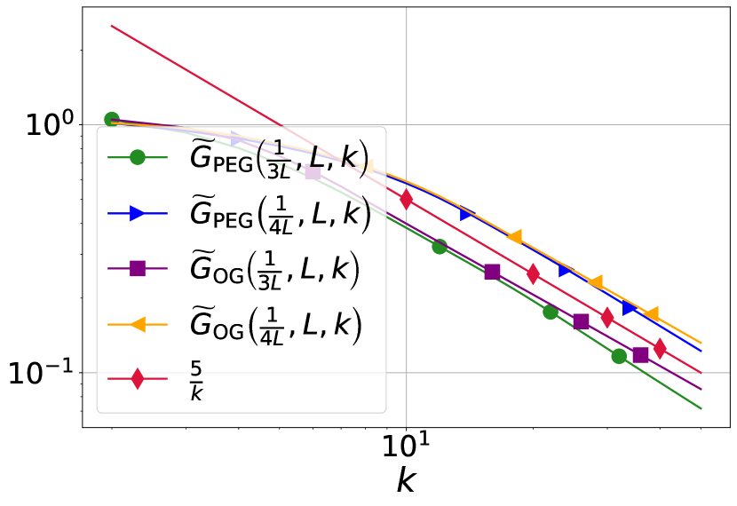
(a) PEPs $\widetilde{G}_{{\sf PEG}}$ and $\widetilde{G}_{{\sf OG}}$.

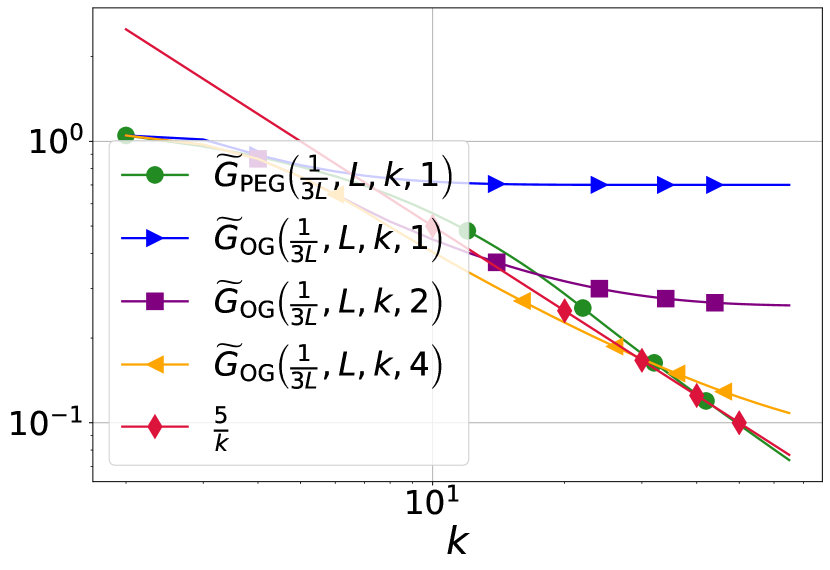
(b) PEPs with distance-$t$ constraints

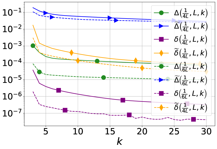
(c) Sq. norm differences

Figure 1: In (a), we report $\widetilde{G}_{{\sf PEG}}(\gamma,L,N)$ and $\widetilde{G}_{{\sf OG}}(\gamma,L,N)$ for different values of $\gamma$ and $N$. In both cases, we observe ${\cal O}(\nicefrac{{1}}{{N}})$ convergence. In (b), we report $\widetilde{G}_{{\sf PEG}}(\gamma,L,N,1)$ and $\widetilde{G}_{{\sf OG}}(\gamma,L,N,t)$ for $t=1,2,4$. It suggest that $\widetilde{G}_{{\sf PEG}}(\gamma,L,N,1)\sim\nicefrac{{1}}{{N}}$ but not $\widetilde{G}_{{\sf OG}}(\gamma,L,N,t)$ (even for $t=4$). Finally, (c) shows how $\Delta(\gamma,L,N),\widetilde{\Delta}(\gamma,L,N),\delta(\gamma,L,N),\widetilde{\delta}(\gamma,L,N)$ evolve as $N$ grows.

Why do we use PEG form instead of OG form?

It is relatively simple to verify that PEG and OG are equivalent [Gidel et al., 2019a, Hsieh et al., 2019]. Moreover, OG can be seen as a simplified version of PEG since OG explicitly uses only one sequence of points, while PEG relies on two sequences. As for PEG, one can consider a PEP for OG:

$$G_{{\sf OG}}(\gamma,L,N)= \max\limits_{\begin{subarray}{c}F,d,x^{*}\\ \tilde{x}^{0},\ldots,\tilde{x}^{N}\end{subarray}} \frac{\|F(\widetilde{x}^{N})\|^{2}}{\|\widetilde{x}^{0}-x^{*}\|^{2}}$$

s.t. $$F\text{ is monotone and $L$-Lipschitz,}$$

$$\widetilde{x}^{0}\in\mathbb{R}^{d},\;\widetilde{x}^{1}=\widetilde{x}^{0}-\gamma F(\widetilde{x}^{0}),$$

$$\widetilde{x}^{k+1}=\widetilde{x}^{k}-2\gamma F(\widetilde{x}^{k})+\gamma F(\widetilde{x}^{k-1}),\text{ for }k=1,\ldots,N-1,$$

as well as its sampled version and the corresponding SDP relaxation, denoted by $\widetilde{G}_{{\sf OG}}(\gamma,L,N)$. Because its sampled version naturally contains only samples of $F$ at the iterates $\{\widetilde{x}^{k}\}_{k=0}^{N}$, the corresponding SDP has about $4$ times less constraints than (2) (recall that (2) also involves Lipschitz and monotonicity inequalities with the iterates $\{x^{k}\}_{k=0}^{N}$). As for $\widetilde{G}_{{\sf PEG}}(\gamma,L,N)$, one can also compute $\widetilde{G}_{{\sf OG}}(\gamma,L,N)$ numerically using SDP solvers, see Fig. 1(a). Those numerical results also suggest that $\widetilde{G}_{{\sf OG}}(\gamma,L,N)={\cal O}(\nicefrac{{1}}{{N}})$ for the different choices of $\gamma$ provided in Fig. 1(a), and $\widetilde{G}_{{\sf PEG}}(\gamma,L,N)$ and $\widetilde{G}_{{\sf OG}}(\gamma,L,N)$ are close to each other for the set of parameters under consideration. Finally, due to the fact that the SDP formulation of $\widetilde{G}_{{\sf OG}}(\gamma,L,N)$ involves less constraints than that of $\widetilde{G}_{{\sf PEG}}(\gamma,L,N)$ while providing very similar results, one might expect that studying $\widetilde{G}_{{\sf OG}}(\gamma,L,N)$ might be simpler.

Convergence proofs of classical first-order optimization methods generally rely on clever combinations of inequalities characterizing the class of problems at hand, and the algorithm. Those inequalities typically involve consecutive iterates and/or a solution $x^{*}$ to the variational problem. For finding a (hopefully) simple proof, let us introduce a few relaxations of $\widetilde{G}_{{\sf PEG}}(\gamma,L,N)$ and $\widetilde{G}_{{\sf OG}}(\gamma,L,N)$, parameterized by some $t\in\mathbb{N}$ and respecitvely denoted by $\widetilde{G}_{{\sf PEG}}(\gamma,L,N,t)$ and $\widetilde{G}_{{\sf OG}}(\gamma,L,N,t)$. Those values respectively correspond to the optimal values of the respective SDP formulations of $\widetilde{G}_{{\sf PEG}}$ and $\widetilde{G}_{{\sf OG}}$ where we removed all constraints corresponding to pairs of iterates $(i,j)$ with $|i-j|>t$. We refer to the remaining constraints as distance-$t$ constraints. For example, distance-$1$ constraints involve monotonicity and Lipschitzness inequalities between two consecutive iterates as well as between the iterates and the solution $x^{*}$ under consideration. As provided by Fig. 1(b), solving the corresponding SDPs for PEG and OG numerically, we observe that $\widetilde{G}_{{\sf PEG}}(\gamma,L,N,1)\sim\nicefrac{{1}}{{N}}$, but the value of $\widetilde{G}_{{\sf OG}}(\gamma,L,N,1)$ seem to stall after a few iterations. This experiment suggests necessity of using the values of $F$ evaluated at $\{x^{k}\}_{k\geq 0}$ for obtaining “simple” proofs involving only inequalities with consecutive iterates.

The norm does not decrease monotonically.

Previous numerical experiments suggest that there exist a proof of ${\cal O}(\nicefrac{{1}}{{N}})$ last-iterate convergence of PEG which uses only inequalities involving consecutive iterates and $x^{*}$. However, the problem of finding the proof remains somehow involved and we did not manage to find analytical expressions (as functions of $\gamma$, $L$, and $N$) to the dual SDP formulation to $\widetilde{G}_{{\sf PEG}}(\gamma,L,N,1)$. Therefore, the following lines aim at finding appropriate Lyapunov function, that is, even looser upper bounds on ${G}_{{\sf PEG}}(\gamma,L,N)$. As a starting point, it is shown in [Gorbunov et al., 2021] that the extragradient method (EG) satisfies $\|F(x^{k+1})\|^{2}\leq\|F(x^{k})\|^{2}$ for all $k\geq 0$ and all monotone Lipschitz operator $F$. Since EG and PEG are very similar methods, it is natural to check whether the same inequality holds for PEG. One way to verify whether this inequality holds is to check nonpositivity of the following PEP:

$$\max\limits_{\begin{subarray}{c}F,d,x^{*}\\ \tilde{x}^{0},\ldots,\tilde{x}^{N}\\ x^{0},\ldots,x^{N}\end{subarray}} \frac{\|F(x^{N+1})\|^{2}-\|F(x^{N})\|^{2}}{\|x^{0}-x^{*}\|^{2}}$$

s.t. $$F\text{ is monotone and $L$-Lipschitz,}$$

$$\widetilde{x}^{0}=x^{0}\in\mathbb{R}^{d},\;x^{1}=x^{0}-\gamma F(x^{0}),$$

$$\widetilde{x}^{k}=x^{k}-\gamma F(\widetilde{x}^{k-1}),\text{ for }k=1,\ldots,N,$$

$$x^{k+1}=x^{k}-\gamma F(\widetilde{x}^{k}),\text{ for }k=1,\ldots,N-1,$$

through its SDP relaxation, whose value is denoted by $\Delta(\gamma,L,N)$. A similar SDP can be formulated for the objective $\|F(\widetilde{x}^{N})\|^{2}-\|F(\widetilde{x}^{N-1})\|^{2}$ and we denote its corresponding optimal value by $\widetilde{\Delta}(\gamma,L,N)$. For convenience, we also define two corresponding SDP formulation whose optimal values are denoted by $\delta(\gamma,L,N)$ and $\widetilde{\delta}(\gamma,L,N)$ and which corresponds to respectively the SDP formulations of $\Delta(\gamma,L,N)$ and $\widetilde{\Delta}(\gamma,L,N)$ where the Lipschitz and monotonicity constraints are replaced by cocoercivity (i.e., $\langle g-h,x-y\rangle\geq 0$ and $\|g-h\|^{2}\leq L^{2}\|x-y\|^{2}$ are replaced by $\|g-h\|^{2}\leq L\langle g-h,x-y\rangle$). Cocoercive operators are both Lipschitz and monotone, and one advantageous property of $\delta(\gamma,L,N)$ and $\widetilde{\delta}(\gamma,L,N)$ is that they are guaranteed to be “tight”. That is, one can construct operators matching the numerical values of respectively $\frac{\|F(x^{N+1})\|^{2}-\|F(x^{N})\|^{2}}{\|x^{0}-x^{*}\|^{2}}$ and $\frac{\|F(\widetilde{x}^{N+1})\|^{2}-\|F(\widetilde{x}^{N})\|^{2}}{\|\widetilde{x}^{0}-x^{*}\|^{2}}$ obtained from the SDPs, see [Ryu et al., 2020, Proposition 2]. Therefore a positive value for $\delta(\gamma,L,N)$ (resp. $\widetilde{\delta}(\gamma,L,N)$) implies the existence of some $L$-Lipschitz monotone $F$ satisfying $\|F(x^{N+1})\|^{2}\geq\|F(x^{N})\|^{2}$ (resp. $\|F(\widetilde{x}^{N+1})\|^{2}\geq\|F(\widetilde{x}^{N})\|^{2}$). Therefore, Fig. 1(c) allows concluding that $\|F(x^{N})\|^{2}$ (resp. $\|F(\widetilde{x}^{N})\|^{2}$) is not a decreasing function of $N$ in general. This fact highlights the difference between EG and PEG in terms of the analysis. However, this experiment also suggests that $\Delta(\gamma,L,N)$ is a decreasing function of $N$ (for some values of $\gamma$).

Therefore, although $\|F(x^{N})\|^{2}$ is not a decreasing function of $N$ for all monotone $L$-Lipschitz operator $F$ and all starting point $x_{0}\in\mathbb{R}^{d}$, it appears that the difference $\|F(x^{N+1})\|^{2}-\|F(x^{N})\|^{2}$ decrease to zero (for all starting point and all operator $F$ satisfying our assumptions) as $N$ grows. Those numerical results suggest that there is a chance to find a non-negative sequence $\{A_{N}\}_{N\geq 0}$ for which $\|F(x^{N+1})\|^{2}+A_{N+1}\leq\|F(x^{N})\|^{2}+A_{N}$. To discover such a sequence, we carefully studied the numerical values of the solutions to the dual SDP for different values of $\gamma$ and $N$ and tried to infer some structure from them. The following section reports the positive results in that direction.

3 Last Iterate Convergence of PEG in the Unconstrained Case

The technique described in the previous section allowed performing an educated trial and error procedure, searching for appropriate potential functions. We finally found a suitable candidate $A_{N}$. In particular, one can numerically check that $\|F(x^{N+1})\|^{2}+2\|F(x^{N+1})-F(\widetilde{x}^{N})\|^{2}\leq\|F(x^{N})\|^{2}+2\|F(x^{N})-F(\widetilde{x}^{N-1})\|^{2}$ for all monotone $L$-Lipschitz $F$ for all tested values of $N$ and $\gamma\leq\nicefrac{{\sqrt{2}}}{{3L}}$. Using the few nonzero dual variables for the problem of verifying this potential function allows reaching the desired proof after a bit of manual cleaning.

Lemma 3.1.

Under Assumption 1, the iterates of PEG with $\gamma>0$ satisfy for any $k>0$,

$$\|F(x^{k+1})\|^{2}+2\|F(x^{k+1})-F(\widetilde{x}^{k})\|^{2} \leq\|F(x^{k})\|^{2}+2\|F(x^{k})-F(\widetilde{x}^{k-1})\|^{2}$$

$$\quad+3\left(L^{2}\gamma^{2}-\frac{2}{9}\right)\|F(\widetilde{x}^{k})-F(\widetilde{x}^{k-1})\|^{2}.$$ (13)

We notice that the last term is non-positive for $0<\gamma\leq\nicefrac{{\sqrt{2}}}{{3L}}$.

Proof.

Since $F$ is monotone and $L$-Lipschitz, we have

$$0 \leq \langle F(x^{k+1})-F(x^{k}),x^{k+1}-x^{k}\rangle,$$

$$\|F(x^{k+1})-F(\widetilde{x}^{k})\|^{2} \leq L^{2}\|x^{k+1}-\widetilde{x}^{k}\|^{2}.$$

By definition of $x^{k+1}$ and $\widetilde{x}^{k}$, we have $x^{k+1}-x^{k}=-\gamma F(\widetilde{x}^{k})$ and $x^{k+1}-\widetilde{x}^{k}=x^{k}-\gamma F(\widetilde{x}^{k})-x^{k}+\gamma F(\widetilde{x}^{k-1})=\gamma\left(F(\widetilde{x}^{k-1})-F(\widetilde{x}^{k})\right)$. Plugging these relations to the above inequalities and dividing the first inequality by $\gamma$, we get

$$0 \leq \langle F(x^{k})-F(x^{k+1}),F(\widetilde{x}^{k})\rangle,$$

$$\|F(x^{k+1})-F(\widetilde{x}^{k})\|^{2} \leq L^{2}\gamma^{2}\|F(\widetilde{x}^{k})-F(\widetilde{x}^{k-1})\|^{2}.$$

Next, we sum up the above inequalities with weights $\lambda_{1}=2$ and $\lambda_{2}=3$ respectively:

$$3\|F(x^{k+1})-F(\widetilde{x}^{k})\|^{2} \leq 2\langle F(x^{k})-F(x^{k+1}),F(\widetilde{x}^{k})\rangle+3L^{2}\gamma^{2}\|F(\widetilde{x}^{k})-F(\widetilde{x}^{k-1})\|^{2}$$

$$\overset{\eqref{eq:inner_product_representation}}{=} \|F(x^{k})\|^{2}+\|F(\widetilde{x}^{k})\|^{2}-\|F(x^{k})-F(\widetilde{x}^{k})\|^{2}$$

$$\quad+\|F(x^{k+1})-F(\widetilde{x}^{k})\|^{2}-\|F(x^{k+1})\|^{2}-\|F(\widetilde{x}^{k})\|^{2}$$

$$\quad+3L^{2}\gamma^{2}\|F(\widetilde{x}^{k})-F(\widetilde{x}^{k-1})\|^{2}.$$

Rearranging the terms, we derive

$$\|F(x^{k+1})\|^{2}+2\|F(x^{k+1})-F(\widetilde{x}^{k})\|^{2} \leq \|F(x^{k})\|^{2}-\|F(x^{k})-F(\widetilde{x}^{k})\|^{2}$$ (14)

$$\quad+3L^{2}\gamma^{2}\|F(\widetilde{x}^{k})-F(\widetilde{x}^{k-1})\|^{2}.$$

To estimate the negative term from the right-hand side of the above inequality we use that $-\|a-b\|^{2}\overset{\eqref{eq:a_minus_b}}{\leq}-\frac{1}{1+\alpha}\|a\|^{2}+\frac{1}{\alpha}\|b\|^{2}$ with $a=F(\widetilde{x}^{k})-F(\widetilde{x}^{k-1})$, $b=F(x^{k})-F(\widetilde{x}^{k-1})$ and $\alpha=\nicefrac{{1}}{{2}}$:

$$-\|F(x^{k})-F(\widetilde{x}^{k})\|^{2} \leq -\frac{2}{3}\|F(\widetilde{x}^{k-1})-F(\widetilde{x}^{k})\|^{2}+2\|F(x^{k})-F(\widetilde{x}^{k-1})\|^{2}.$$

Plugging the above inequality in (14), we obtain

$$\|F(x^{k+1})\|^{2}+2\|F(x^{k+1})-F(\widetilde{x}^{k})\|^{2} \leq \|F(x^{k})\|^{2}+2\|F(x^{k})-F(\widetilde{x}^{k-1})\|^{2}$$

$$\quad+3\left(L^{2}\gamma^{2}-\frac{2}{9}\right)\|F(\widetilde{x}^{k})-F(\widetilde{x}^{k-1})\|^{2},$$

which finishes the proof. ∎

Using this lemma we then show the last-iterate convergence rate of PEG.

Theorem 1.

Let operator $F$ be monotone and $L$-Lipschitz. Then for all $k\geq 0$ the iterates of PEG with $\gamma\leq\nicefrac{{1}}{{3L}}$ satisfy $\Phi_{k+1}\leq\Phi_{k}$ with $\Phi_{k}$ defined as

$$\Phi_{k}=\|x^{k}-x^{*}\|^{2}+\frac{k+32}{3}\gamma^{2}\left(\|F(x^{k})\|^{2}+2\|F(x^{k})-F(\widetilde{x}^{k-1})\|^{2}\right).$$ (15)

In particular, for all $N\geq 0$ and $\gamma\leq\nicefrac{{1}}{{3L}}$ the above formula implies

$$\|F(x^{N})\|^{2}\leq\frac{3(1+32L^{2}\gamma^{2})\|x^{0}-x^{*}\|^{2}}{\gamma^{2}(N+32)},\quad\texttt{Gap}_{F}(x^{k})\leq\frac{2\sqrt{41}(1+32L^{2}\gamma^{2})\|x^{0}-x^{*}\|^{2}}{\gamma\sqrt{3N+96}}.$$ (16)

As we write before, in contrast to Golowich et al. [2020a], our results does not rely on the Lipschitzness of $\nabla F(x)$. Moreover, even when $\nabla F(x)$ is assumed to be $\Lambda$-Lipschitz, our result improve upon Golowich et al. [2020a] in certain regimes. In particular, if $\Lambda\|x^{0}-x^{*}\|\gg L$, which is typically the case (e.g., see Appendix B from Gorbunov et al. [2021] for the details), the constants in our upper bounds are significantly smaller and even when $\Lambda\|x^{0}-x^{*}\|\ll L$ our result allows for stepsizes $50$ times larger with a improvement by a factor $\approx 10^{6}$ in terms of convergence rate for $\|F(x^{k})\|^{2}$.

Next, our analysis significantly differs from the previous known one from Golowich et al. [2020a]. In particular, using Lipschitzness of Jacobian, Golowich et al. [2020a] derive that $\|F(\widetilde{x}^{N})\|^{2}$ is not much larger than $\min_{k=0,\ldots,N}\|F(x^{k})\|^{2}$, which instantly implies a ${\cal O}(\nicefrac{{1}}{{N}})$ last-iterate convergence rate after applying standard results for the best-iterate convergence of PEG. In contrast, we do not derive any connections between the best and the last iterates of PEG and directly rely on the fact that $\|F(x^{k})\|^{2}+2\|F(x^{k})-F(\widetilde{x}^{k-1})\|^{2}$ is a decreasing function of $k$, i.e., on Lemma 3.1.

We also remark that the derived upper bounds are worse than those that we obtained numerically and reported in Fig. 1(a). For example, when $N=50$ and $\gamma=\nicefrac{{1}}{{3L}}$ the upper bound on $\|F(x^{N})\|^{2}$ from Theorem 1 is $\approx 20$ times worse than the upper bound found numerically. Since our goal was in deriving a simple proof of the ${\cal O}(\nicefrac{{1}}{{N}})$ rate, we did not try to improve the multiplicative constants in the final results. We also do not plot the curve corresponding to the upper bound on $\|F(x^{N})\|^{2}$ from Theorem 1 for the sake of readability of Fig. 1(a).

4 Last Iterate Convergence of PEG in the Constrained Case

In this section, we extend the last-iterate convergence rates proven in Theorem 1 to the constrained case. Such an extension is not straightforward because the convergence criterion considered in the unconstrained case cannot be used anymore in the constrained case. That is, Lemma 3.1 is not valid anymore and cannot be easily adapted to the constrained case: norm of the operator $\|F(x^{k})\|$ does not necessarily converge to zero since $F(x^{*})\neq 0$ in general. However, to find new potential function we used the same techniques as in the unconstrained case. This search led us to the following result.

Lemma 4.1.

Under Assumption 1, the iterates of Proj-PEG with $\gamma>0$ satisfy for any $k>0$,

$$\Psi_{k+1}\leq\Psi_{k}-\left(1-5L^{2}\gamma^{2}\right)\|x^{k+1}-\widetilde{x}^{k}\|^{2}-\gamma^{2}\|F(x^{k+1})-F(\widetilde{x}^{k})\|^{2},$$ (17)

where $\Psi_{k}=\|x^{k}-x^{k-1}\|^{2}+\|x^{k}-x^{k-1}-2\gamma(F(x^{k})-F(\widetilde{x}^{k-1}))\|^{2}$.

Proof sketch.

Numerically we discovered that to prove this result it is sufficient to sum up constraints corresponding to the monotonicity at $(x^{k},x^{k+1})$, Lipschitzness at $(x^{k+1},\widetilde{x}^{k})$, and projections properties for the pairs $(x^{k+1},x^{k}),(x^{k},x^{k+1}),(x^{k},\widetilde{x}^{k}),(\widetilde{x}^{k},x^{k+1})$, with weights $4\gamma,5\gamma^{2},4,2,2,2$ respectively. After that, it remains to rearrange the terms and apply standard inequalities from Appendix A to derive the result. See the detailed proof in Appendix C. ∎

This lemma is critically different from Lemma 3.1 since in the unconstrained case the potential from Lemma 4.1 reduces to $\Psi_{k}=\|F(\tilde{x}^{k-1})\|^{2}+\|F(\tilde{x}^{k-1})-2\gamma(F(x^{k})-F(\widetilde{x}^{k-1}))\|^{2}$. Moreover, as one can see from the next result, using the potential from Lemma 4.1, we obtain the proof valid for slightly smaller stepsize than in the unconstrained case (see also Appendix D for the numerical verification of the rate).

Theorem 2.

Under Assumption 1, the iterates of Proj-PEG with $\gamma\leq\nicefrac{{1}}{{4L}}$ satisfy $\Phi_{k+1}\leq\Phi_{k}\,,\;k\geq 2$ with $\Phi_{k}$ defined as

$$\Phi_{k}=\|x^{k}-x^{*}\|^{2}+\frac{1}{16}\|\widetilde{x}^{k-1}-\widetilde{x}^{k-2}\|^{2}+\frac{3k+32}{24}\Psi_{k},$$ (18)

where $\Psi_{k}=\|x^{k}-x^{k-1}\|^{2}+\|x^{k}-x^{k-1}-2\gamma(F(x^{k})-F(\widetilde{x}^{k-1}))\|^{2}$. In particular, it implies

$$\|x^{N}-x^{N-1}\|^{2}\leq\frac{24H_{0,\gamma}^{2}}{3N+32},\quad\texttt{Gap}_{F}(x^{N})\leq\frac{8\sqrt{3}H_{0,\gamma}\cdot H_{0}}{\gamma\sqrt{3N+32}},\quad\forall N\geq 2\,,$$ (19)

where $H_{0},H_{0,\gamma}>0$ are such that $H_{0,\gamma}^{2}=2(1+3\gamma^{2}L^{2}+4\gamma^{4}L^{4})\|x^{0}-x^{*}\|^{2}+\left(\frac{41}{12}+\frac{19}{3}\gamma^{2}L^{2}\right)\gamma^{2}\|F(x^{0})\|^{2}$, $H_{0}^{2}=3\|x^{0}-x^{*}\|^{2}+\tfrac{1}{30L^{2}}\|F(x^{0})\|^{2}$.

This result extends last-iterate convergence of Proj-PEG to the constrained case. The closest result in the literature is Cai et al. [2022, Theorem 3] that gives a last-iterate convergence result for EG in terms of the tangent residual and gap function. Moreover, we show a ${\cal O}(\nicefrac{{1}}{{N}})$ last-iterate convergence result for the residuals, which is stronger than the result in Cai et al. [2022, Theorem 3]. Moreover, our results justify that higher-order SOS programs (with polynomials of degree larger than $2$) used by Cai et al. [2022] are not required to derive tight last-iterate convergence results for Proj-PEG. We believe that this is the case for other EG-like methods and similar rates could be proven for the residuals of these methods as well (see Appendix D for preliminary results supporting this claim).

5 Discussion

In this work, we leveraged the performance estimation problem framework to show the last-iterate convergence of PEG of monotone and Lipschitz operators both in the constrained and unconstrained cases. These results answer some important questions that remained open until now in the variational inequality literature showcasing the appealing properties of extrapolation-based methods. However, important open questions remain such as last-iterate convergence rates for stochastic methods for monotone and Lipschitz variational inequalities or a better understanding of the dynamics in non-monotone cases that occur in machine learning applications. Finally, the results obtained for PEG in this work have worse multiplicative constants and more restrictive range of stepsizes than those obtained for EG Gorbunov et al. [2021], Cai et al. [2022]. It would be interesting to address this discrepancy in the future work.

Checklist

1. For all authors…

   1. Do the main claims made in the abstract and introduction accurately reflect the paper’s contributions and scope? [Yes]

   2. Did you describe the limitations of your work? [Yes] See §1 and §5

   3. Did you discuss any potential negative societal impacts of your work? [N/A]

   4. Have you read the ethics review guidelines and ensured that your paper conforms to them? [N/A]

2. If you are including theoretical results…

   1. Did you state the full set of assumptions of all theoretical results? [Yes] See §1, §3, and §4

   2. Did you include complete proofs of all theoretical results? [Yes] See §3 and Appendices B and C

3. If you ran experiments…

   1. Did you include the code, data, and instructions needed to reproduce the main experimental results (either in the supplemental material or as a URL)? [Yes] Codes are publicly available: https://github.com/eduardgorbunov/potentials_and_last_iter_convergence_for_VIPs

   2. Did you specify all the training details (e.g., data splits, hyperparameters, how they were chosen)? [N/A]

   3. Did you report error bars (e.g., with respect to the random seed after running experiments multiple times)? [N/A]

   4. Did you include the total amount of compute and the type of resources used (e.g., type of GPUs, internal cluster, or cloud provider)? [N/A]

4. If you are using existing assets (e.g., code, data, models) or curating/releasing new assets…

   1. If your work uses existing assets, did you cite the creators? [N/A]

   2. Did you mention the license of the assets? [N/A]

   3. Did you include any new assets either in the supplemental material or as a URL? [N/A]

   4. Did you discuss whether and how consent was obtained from people whose data you’re using/curating? [N/A]

   5. Did you discuss whether the data you are using/curating contains personally identifiable information or offensive content? [N/A]

5. If you used crowdsourcing or conducted research with human subjects…

   1. Did you include the full text of instructions given to participants and screenshots, if applicable? [N/A]

   2. Did you describe any potential participant risks, with links to Institutional Review Board (IRB) approvals, if applicable? [N/A]

   3. Did you include the estimated hourly wage paid to participants and the total amount spent on participant compensation? [N/A]

Appendix A Useful Facts

Standard inequalities.

For all $a,b\in\mathbb{R}^{d}$ and $\alpha>0$ the following relations hold:

$$2\langle a,b\rangle = \|a\|^{2}+\|b\|^{2}-\|a-b\|^{2},$$ (20)

$$\|a+b\|^{2} \leq (1+\alpha)\|a\|^{2}+(1+\alpha^{-1})\|b\|^{2},$$ (21)

$$-\|a-b\|^{2} \leq -\frac{1}{1+\alpha}\|a\|^{2}+\frac{1}{\alpha}\|b\|^{2}.$$ (22)

Auxiliary results.

In the analysis of Proj-PEG, we use two lemmas from Gidel et al. [2019a].

Lemma A.1 (Lemma 5 from Gidel et al. [2019a]).

Let operator $F$ be $L$-Lipschitz. Then for all $k\geq 1$ the iterates of Proj-PEG with $\gamma>0$ satisfy

$$2\gamma\langle F(\widetilde{x}^{k}),\widetilde{x}^{k}-x^{*}\rangle\leq\|x^{k}-x^{*}\|^{2}-\|x^{k+1}-x^{*}\|^{2}-\|\widetilde{x}^{k}-x^{k}\|^{2}+\gamma^{2}L^{2}\|\widetilde{x}^{k}-\widetilde{x}^{k-1}\|^{2}.$$ (23)

Lemma A.2 (Lemma 6 from Gidel et al. [2019a]).

Let operator $F$ be $L$-Lipschitz. Then for all $k\geq 2$ the iterates of Proj-PEG with $\gamma>0$ satisfy

$$\|\widetilde{x}^{k}-\widetilde{x}^{k-1}\|^{2}\leq 4\|\widetilde{x}^{k}-x^{k}\|^{2}+4\gamma^{2}L^{2}\|\widetilde{x}^{k-1}-\widetilde{x}^{k-2}\|^{2}-\|\widetilde{x}^{k}-\widetilde{x}^{k-1}\|^{2}.$$ (24)

Appendix B Proof of Theorem 1

Let us first recall Theorem 1.

Theorem 1.

Let operator $F$ be monotone and $L$-Lipschitz. Then for all $k\geq 0$ the iterates of PEG with $\gamma\leq\nicefrac{{1}}{{3L}}$ satisfy $\Phi_{k+1}\leq\Phi_{k}$ with $\Phi_{k}$ defined as

$$\Phi_{k}=\|x^{k}-x^{*}\|^{2}+\frac{k+32}{3}\gamma^{2}\left(\|F(x^{k})\|^{2}+2\|F(x^{k})-F(\widetilde{x}^{k-1})\|^{2}\right).$$ (25)

In particular, for all $N\geq 0$ and $\gamma\leq\nicefrac{{1}}{{3L}}$ the above formula implies

$$\|F(x^{N})\|^{2}\leq\frac{3(1+32L^{2}\gamma^{2})\|x^{0}-x^{*}\|^{2}}{\gamma^{2}(N+32)},\quad\texttt{Gap}_{F}(x^{k})\leq\frac{2\sqrt{41}(1+32L^{2}\gamma^{2})\|x^{0}-x^{*}\|^{2}}{\gamma\sqrt{3N+96}}.$$ (26)

Proof.

We start with the upper bound for $\|x^{k+1}-x^{*}\|^{2}$:

$$\|x^{k+1}-x^{*}\|^{2} = \|x^{k}-x^{*}-\gamma F(\widetilde{x}^{k})\|^{2}$$

$$= \|x^{k}-x^{*}\|^{2}-2\gamma\langle x^{k}-x^{*},F(\widetilde{x}^{k})\rangle+\gamma^{2}\|F(\widetilde{x}^{k})\|^{2}$$

$$= \|x^{k}-x^{*}\|^{2}-2\gamma\langle\widetilde{x}^{k}-x^{*},F(\widetilde{x}^{k})\rangle-2\gamma\langle x^{k}-\widetilde{x}^{k},F(\widetilde{x}^{k})\rangle+\gamma^{2}\|F(\widetilde{x}^{k})\|^{2}.$$

Since $F$ is monotone, we have $\langle\widetilde{x}^{k}-x^{*},F(\widetilde{x}^{k})\rangle\geq 0$. Moreover, the update rule for PEG implies $\langle x^{k}-\widetilde{x}^{k},F(\widetilde{x}^{k})\rangle=\gamma\langle F(\widetilde{x}^{k-1}),F(\widetilde{x}^{k})\rangle$. Using these relations, we continue our derivation as

$$\|x^{k+1}-x^{*}\|^{2} \leq \|x^{k}-x^{*}\|^{2}-2\gamma^{2}\langle F(\widetilde{x}^{k-1}),F(\widetilde{x}^{k})\rangle+\gamma^{2}\|F(\widetilde{x}^{k})\|^{2}$$

$$= \|x^{k}-x^{*}\|^{2}+\gamma^{2}\|F(\widetilde{x}^{k-1})-F(\widetilde{x}^{k})\|^{2}-\gamma^{2}\|F(\widetilde{x}^{k-1})\|^{2}.$$

Next, we sum up the above inequality with $(\nicefrac{{(k+33)\gamma^{2}}}{{3}})$-multiple of (13) and use the definition of $\Phi_{k}$ from (25):

$$\Phi_{k+1} \leq \|x^{k}-x^{*}\|^{2}+\gamma^{2}\|F(\widetilde{x}^{k-1})-F(\widetilde{x}^{k})\|^{2}-\gamma^{2}\|F(\widetilde{x}^{k-1})\|^{2}$$

$$\quad+\frac{(k+33)\gamma^{2}}{3}\left(\|F(x^{k})\|^{2}+2\|F(x^{k})-F(\widetilde{x}^{k-1})\|^{2}\right)$$

$$\quad+(k+33)\gamma^{2}\left(L^{2}\gamma^{2}-\frac{2}{9}\right)\|F(\widetilde{x}^{k})-F(\widetilde{x}^{k-1})\|^{2}$$

$$\overset{\gamma\leq\nicefrac{{1}}{{3L}}}{\leq} \Phi_{k}+\frac{\gamma^{2}}{3}\left(\|F(x^{k})\|^{2}+2\|F(x^{k})-F(\widetilde{x}^{k-1})\|^{2}\right)-\gamma^{2}\|F(\widetilde{x}^{k-1})\|^{2}$$

$$\quad+\gamma^{2}\left(1-\frac{k+33}{9}\right)\|F(\widetilde{x}^{k})-F(\widetilde{x}^{k-1})\|^{2}.$$

Applying $\|F(x^{k})\|^{2}\leq 2\|F(\widetilde{x}^{k-1})\|^{2}+2\|F(x^{k})-F(\widetilde{x}^{k-1})\|^{2}$ and then $\|F(x^{k})-F(\widetilde{x}^{k-1})\|^{2}\leq 2\|F(x^{k})-F(\widetilde{x}^{k})\|^{2}+2\|F(\widetilde{x}^{k})-F(\widetilde{x}^{k-1})\|^{2}\overset{\eqref{eq:Lipschitzness}}{\leq}2L^{2}\|x^{k}-\widetilde{x}^{k}\|^{2}+2\|F(\widetilde{x}^{k})-F(\widetilde{x}^{k-1})\|^{2}=2L^{2}\gamma^{2}\|F(\widetilde{x}^{k-1})\|^{2}+2\|F(\widetilde{x}^{k})-F(\widetilde{x}^{k-1})\|^{2}\leq\tfrac{2}{9}\|F(\widetilde{x}^{k-1})\|^{2}+2\|F(\widetilde{x}^{k})-F(\widetilde{x}^{k-1})\|^{2}$, we derive

$$\Phi_{k+1} \leq \Phi_{k}+\frac{8}{3}\gamma^{2}\|F(x^{k})-F(\widetilde{x}^{k-1})\|^{2}-\frac{\gamma^{2}}{3}\|F(\widetilde{x}^{k-1})\|^{2}$$

$$\quad+\gamma^{2}\left(1-\frac{k+33}{9}\right)\|F(\widetilde{x}^{k})-F(\widetilde{x}^{k-1})\|^{2}$$

$$\leq \Phi_{k}+\gamma^{2}\left(\frac{8}{27}-\frac{1}{3}\right)\|F(\widetilde{x}^{k-1})\|^{2}+\gamma^{2}\left(\frac{11}{3}-\frac{k+33}{9}\right)\|F(\widetilde{x}^{k})-F(\widetilde{x}^{k-1})\|^{2}$$

$$\leq \Phi_{k},$$

where in the last step we use $k\geq 0$. In other words, we proved that $\Phi_{k}$ defined in (25) is a potential for (PEG). In particular, $\Phi_{k}\leq\Phi_{k-1}\leq\ldots\leq\Phi_{0}=\|x^{0}-x^{*}\|^{2}+32\gamma^{2}\|F(x^{0})\|^{2}\overset{\eqref{eq:Lipschitzness}}{\leq}(1+32L^{2}\gamma^{2})\|x^{0}-x^{*}\|^{2}$ (here we use our convention: $F(\widetilde{x}^{-1})=0$) and all terms in $\Phi_{k}$ are non-negative. These facts imply that for all $k\geq 0$

$$\|F(x^{k})\|^{2} \leq \frac{3}{\gamma^{2}(k+32)}\Phi_{k}\leq\frac{3(1+32L^{2}\gamma^{2})\|x^{0}-x^{*}\|^{2}}{\gamma^{2}(k+32)},$$ (27)

$$\|x^{k}-x^{*}\|^{2} \leq \Phi_{k}\leq(1+32L^{2}\gamma^{2})\|x^{0}-x^{*}\|^{2}.$$ (28)

That is, we obtained the first part of (26). The second part of (26) follows from the monotonicity of $F$ and the above inequalities:

$$\texttt{Gap}_{F}(x^{k}) = \max\limits_{y\in\mathbb{R}^{d}:\|y-x^{*}\|\leq\tfrac{\sqrt{41}}{3}\|x^{0}-x^{*}\|}\langle F(y),x^{k}-y\rangle$$

$$\overset{\eqref{eq:Lipschitzness}}{\leq} \max\limits_{y\in\mathbb{R}^{d}:\|y-x^{*}\|\leq\tfrac{\sqrt{41}}{3}\|x^{0}-x^{*}\|}\langle F(x^{k}),x^{k}-y\rangle$$

$$\leq \|F(x^{k})\|\cdot\max\limits_{y\in\mathbb{R}^{d}:\|y-x^{*}\|\leq\tfrac{\sqrt{41}}{3}\|x^{0}-x^{*}\|}\|x^{k}-y\|$$

$$\leq \|F(x^{k})\|\left(\|x^{k}-x^{*}\|+\tfrac{\sqrt{41}}{3}\|x^{0}-x^{*}\|\right)$$

$$\overset{\eqref{eq:technical_2},\eqref{eq:technical_3}}{\leq} \frac{2\sqrt{41}(1+32L^{2}\gamma^{2})\|x^{0}-x^{*}\|^{2}}{\gamma\sqrt{3k+96}}.$$

∎

Appendix C Proof of Theorem 2

Let us start with an important lemma.

Lemma 4.1.

Under Assumption 1, the iterates of Proj-PEG with $\gamma>0$ satisfy for any $k>0$,

$$\Psi_{k+1}\leq\Psi_{k}-\left(1-5L^{2}\gamma^{2}\right)\|x^{k+1}-\widetilde{x}^{k}\|^{2}-\gamma^{2}\|F(x^{k+1})-F(\widetilde{x}^{k})\|^{2},$$ (29)

where $\Psi_{k}=\|x^{k}-x^{k-1}\|^{2}+\|x^{k}-x^{k-1}-2\gamma(F(x^{k})-F(\widetilde{x}^{k-1}))\|^{2}$.

Proof.

Since $F$ is monotone and $L$-Lipschitz, we have

$$0 \leq \langle F(x^{k+1})-F(x^{k}),x^{k+1}-x^{k}\rangle,$$ (30)

$$\|F(x^{k+1})-F(\widetilde{x}^{k})\|^{2} \leq L^{2}\|x^{k+1}-\widetilde{x}^{k}\|^{2}.$$ (31)

Taking into account relations $x^{k+1}=\mathop{\mathrm{proj}}\nolimits[x^{k}-\gamma F(\widetilde{x}^{k})],x^{k}=\mathop{\mathrm{proj}}\nolimits[x^{k-1}-\gamma F(\widetilde{x}^{k-1})],\widetilde{x}^{k}=\mathop{\mathrm{proj}}\nolimits[x^{k}-\gamma F(\widetilde{x}^{k-1})]$ and properties of the projection on a convex closed set, we also obtain

$$\langle x^{k}-\gamma F(\widetilde{x}^{k})-x^{k+1},x^{k}-x^{k+1}\rangle \leq 0,$$ (32)

$$\langle x^{k-1}-\gamma F(\widetilde{x}^{k-1})-x^{k},x^{k+1}-x^{k}\rangle \leq 0,$$ (33)

$$\langle x^{k-1}-\gamma F(\widetilde{x}^{k-1})-x^{k},\widetilde{x}^{k}-x^{k}\rangle \leq 0,$$ (34)

$$\langle x^{k}-\gamma F(\widetilde{x}^{k-1})-\widetilde{x}^{k},x^{k+1}-\widetilde{x}^{k}\rangle \leq 0.$$ (35)

Summing up inequalities (30)-(35) with weights $4\gamma,5\gamma^{2},4,2,2,2$ respectively, we get

$$5\gamma^{2}\|F(x^{k+1})-F(\widetilde{x}^{k})\|^{2} \leq 5\gamma^{2}L^{2}\|x^{k+1}-\widetilde{x}^{k}\|^{2}+4\gamma\langle F(x^{k+1})-F(x^{k}),x^{k+1}-x^{k}\rangle$$

$$\quad-4\langle x^{k}-\gamma F(\widetilde{x}^{k})-x^{k+1},x^{k}-x^{k+1}\rangle$$

$$\quad-2\langle x^{k-1}-\gamma F(\widetilde{x}^{k-1})-x^{k},x^{k+1}-x^{k}\rangle$$

$$\quad-2\langle x^{k-1}-\gamma F(\widetilde{x}^{k-1})-x^{k},\widetilde{x}^{k}-x^{k}\rangle$$

$$\quad-2\langle x^{k}-\gamma F(\widetilde{x}^{k-1})-\widetilde{x}^{k},x^{k+1}-\widetilde{x}^{k}\rangle$$

$$= 5\gamma^{2}L^{2}\|x^{k+1}-\widetilde{x}^{k}\|^{2}+4\gamma\langle F(x^{k+1})-F(x^{k}),x^{k+1}-x^{k}\rangle$$

$$\quad-4\|x^{k+1}-x^{k}\|^{2}+4\gamma\langle F(\widetilde{x}^{k}),x^{k}-x^{k+1}\rangle$$

$$\quad+4\gamma\langle F(\widetilde{x}^{k-1}),x^{k+1}-x^{k}\rangle-2\langle x^{k-1}-x^{k},x^{k+1}-x^{k}\rangle$$

$$\quad-2\langle x^{k-1}-x^{k},\widetilde{x}^{k}-x^{k}\rangle-2\langle x^{k}-\widetilde{x}^{k},x^{k+1}-\widetilde{x}^{k}\rangle$$

$$= 5\gamma^{2}L^{2}\|x^{k+1}-\widetilde{x}^{k}\|^{2}+4\gamma\langle F(x^{k+1})-F(\widetilde{x}^{k}),x^{k+1}-x^{k}\rangle$$

$$\quad-4\|x^{k+1}-x^{k}\|^{2}-4\gamma\langle F(x^{k})-F(\widetilde{x}^{k-1}),x^{k+1}-x^{k}\rangle$$

$$\quad+\|x^{k-1}-x^{k}\|^{2}+\|x^{k+1}-x^{k}\|^{2}-\|x^{k+1}+x^{k-1}-2x^{k}\|^{2}$$

$$\quad+\|x^{k-1}-\widetilde{x}^{k}\|^{2}-\|x^{k-1}-x^{k}\|^{2}-\|\widetilde{x}^{k}-x^{k}\|^{2}$$

$$\quad+\|x^{k}-x^{k+1}\|^{2}-\|x^{k}-\widetilde{x}^{k}\|^{2}-\|x^{k+1}-\widetilde{x}^{k}\|^{2}.$$

Next, we rearrange the terms and use $\Psi_{k}=\|x^{k}-x^{k-1}\|^{2}+\|x^{k}-x^{k-1}-2\gamma(F(x^{k})-F(\widetilde{x}^{k-1}))\|^{2}=2\|x^{k}-x^{k-1}\|^{2}-4\gamma\langle x^{k}-x^{k-1},F(x^{k})-F(\widetilde{x}^{k-1})\rangle+4\gamma^{2}\|F(x^{k})-F(\widetilde{x}^{k-1})\|^{2}$:

$$\Psi_{k+1} \leq -(1-5\gamma^{2}L^{2})\|x^{k+1}-\widetilde{x}^{k}\|^{2}-4\gamma\langle F(x^{k})-F(\widetilde{x}^{k-1}),x^{k+1}-x^{k}\rangle$$

$$\quad-\|x^{k+1}+x^{k-1}-2x^{k}\|^{2}+\|x^{k-1}-\widetilde{x}^{k}\|^{2}-2\|\widetilde{x}^{k}-x^{k}\|^{2}$$

$$\quad-\gamma^{2}\|F(x^{k+1})-F(\widetilde{x}^{k})\|^{2}$$

$$= \Psi_{k}-2\|x^{k}-x^{k-1}\|^{2}-2\langle 2\gamma(F(x^{k})-F(\widetilde{x}^{k-1})),x^{k+1}+x^{k-1}-2x^{k}\rangle$$

$$\quad-4\gamma^{2}\|F(x^{k})-F(\widetilde{x}^{k-1})\|^{2}-(1-5\gamma^{2}L^{2})\|x^{k+1}-\widetilde{x}^{k}\|^{2}$$

$$\quad-\|x^{k+1}+x^{k-1}-2x^{k}\|^{2}+\|x^{k-1}-\widetilde{x}^{k}\|^{2}-2\|\widetilde{x}^{k}-x^{k}\|^{2}$$

$$\quad-\gamma^{2}\|F(x^{k+1})-F(\widetilde{x}^{k})\|^{2}.$$

Using standard inequalities $2\langle a,b\rangle\leq\|a\|^{2}+\|b\|^{2}$, $\|a+b\|^{2}\leq 2\|a\|^{2}+2\|b\|^{2}$, $a,b\in\mathbb{R}^{d}$, we derive

$$\Psi_{k+1} \leq \Psi_{k}-2\|x^{k}-x^{k-1}\|^{2}+4\gamma^{2}\|F(x^{k})-F(\widetilde{x}^{k-1})\|^{2}+\|x^{k+1}+x^{k-1}-2x^{k}\|^{2}$$

$$\quad-4\gamma^{2}\|F(x^{k})-F(\widetilde{x}^{k-1})\|^{2}-(1-5\gamma^{2}L^{2})\|x^{k+1}-\widetilde{x}^{k}\|^{2}$$

$$\quad-\|x^{k+1}+x^{k-1}-2x^{k}\|^{2}+2\|x^{k-1}-x^{k}\|^{2}+2\|x^{k}-\widetilde{x}^{k}\|^{2}-2\|\widetilde{x}^{k}-x^{k}\|^{2}$$

$$\quad-\gamma^{2}\|F(x^{k+1})-F(\widetilde{x}^{k})\|^{2}$$

$$= \Psi_{k}-(1-5\gamma^{2}L^{2})\|x^{k+1}-\widetilde{x}^{k}\|^{2}-\gamma^{2}\|F(x^{k+1})-F(\widetilde{x}^{k})\|^{2},$$

which finishes the proof. ∎

We can now prove the main theorem.

Theorem 2.

Under Assumption 1, the iterates of Proj-PEG with $\gamma\leq\nicefrac{{1}}{{4L}}$ satisfy $\Phi_{k+1}\leq\Phi_{k}\,,\;k\geq 2$ with $\Phi_{k}$ defined as

$$\Phi_{k}=\|x^{k}-x^{*}\|^{2}+\frac{1}{16}\|\widetilde{x}^{k-1}-\widetilde{x}^{k-2}\|^{2}+\frac{3k+32}{24}\Psi_{k},$$ (36)

where $\Psi_{k}=\|x^{k}-x^{k-1}\|^{2}+\|x^{k}-x^{k-1}-2\gamma(F(x^{k})-F(\widetilde{x}^{k-1}))\|^{2}$. In particular, it implies

$$\|x^{N}-x^{N-1}\|^{2}\leq\frac{24H_{0,\gamma}^{2}}{3N+32},\quad\texttt{Gap}_{F}(x^{N})\leq\frac{8\sqrt{3}H_{0,\gamma}\cdot H_{0}}{\gamma\sqrt{3N+32}},\quad\forall N\geq 2\,,$$ (37)

where $H_{0},H_{0,\gamma}>0$ are such that $H_{0,\gamma}^{2}=2(1+3\gamma^{2}L^{2}+4\gamma^{4}L^{4})\|x^{0}-x^{*}\|^{2}+\left(\frac{41}{12}+\frac{19}{3}\gamma^{2}L^{2}\right)\gamma^{2}\|F(x^{0})\|^{2}$, $H_{0}^{2}=3\|x^{0}-x^{*}\|^{2}+\tfrac{1}{30L^{2}}\|F(x^{0})\|^{2}$.

Proof.

Lemma A.1 implies

$$0 \leq 2\gamma\langle F(x^{*}),\widetilde{x}^{k}-x^{*}\rangle\leq 2\gamma\langle F(\widetilde{x}^{k}),\widetilde{x}^{k}-x^{*}\rangle$$

$$\leq \|x^{k}-x^{*}\|^{2}-\|x^{k+1}-x^{*}\|^{2}-\|\widetilde{x}^{k}-x^{k}\|^{2}+\gamma^{2}L^{2}\|\widetilde{x}^{k}-\widetilde{x}^{k-1}\|^{2}.$$

Together with Lemma A.2 it gives

$$\|x^{k+1}-x^{*}\|^{2}+\frac{1}{16}\|\widetilde{x}^{k}-\widetilde{x}^{k-1}\|^{2} \leq \|x^{k}-x^{*}\|^{2}-\|\widetilde{x}^{k}-x^{k}\|^{2}+\gamma^{2}L^{2}\|\widetilde{x}^{k}-\widetilde{x}^{k-1}\|^{2}$$

$$\quad+\frac{1}{16}\|\widetilde{x}^{k-1}-\widetilde{x}^{k-2}\|^{2}-\frac{1}{16}\|\widetilde{x}^{k-1}-\widetilde{x}^{k-2}\|^{2}$$

$$\quad+\frac{1}{4}\|\widetilde{x}^{k}-x^{k}\|^{2}+\frac{\gamma^{2}L^{2}}{4}\|\widetilde{x}^{k-1}-\widetilde{x}^{k-2}\|^{2}$$

$$\quad-\frac{1}{16}\|\widetilde{x}^{k}-\widetilde{x}^{k-1}\|^{2}$$

$$= \|x^{k}-x^{*}\|^{2}+\frac{1}{16}\|\widetilde{x}^{k-1}-\widetilde{x}^{k-2}\|^{2}-\frac{3}{4}\|\widetilde{x}^{k}-x^{k}\|^{2}$$

$$\quad-\frac{1-16\gamma^{2}L^{2}}{16}\|\widetilde{x}^{k}-\widetilde{x}^{k-1}\|^{2}$$

$$\quad-\frac{1-4\gamma^{2}L^{2}}{16}\|\widetilde{x}^{k-1}-\widetilde{x}^{k-2}\|^{2}$$

$$\leq \|x^{k}-x^{*}\|^{2}+\frac{1}{16}\|\widetilde{x}^{k-1}-\widetilde{x}^{k-2}\|^{2}-\frac{3}{4}\|\widetilde{x}^{k}-x^{k}\|^{2},$$

where in the last inequality we apply $\gamma\leq\nicefrac{{1}}{{4L}}$. Combining the above inequality with (29), we derive

$$\Phi_{k+1} \leq \Phi_{k}+\frac{3}{24}\left(\|x^{k+1}-x^{k}\|^{2}+\|x^{k+1}-x^{k}-2\gamma(F(x^{k+1})-F(\widetilde{x}^{k}))\|^{2}\right)$$

$$\quad-\frac{3}{4}\|\widetilde{x}^{k}-x^{k}\|^{2}-\frac{3k+32}{24}\left((1-5\gamma^{2}L^{2})\|x^{k+1}-\widetilde{x}^{k}\|^{2}+\gamma^{2}\|F(x^{k+1})-F(\widetilde{x}^{k})\|^{2}\right)$$

$$\leq \Phi_{k}+\frac{1}{8}\left(3\|x^{k+1}-x^{k}\|^{2}+8\gamma^{2}\|F(x^{k+1})-F(\widetilde{x}^{k})\|^{2}\right)$$

$$\quad-\frac{3}{4}\|\widetilde{x}^{k}-x^{k}\|^{2}-\frac{4}{3}\left(\frac{9}{16}\|x^{k+1}-\widetilde{x}^{k}\|^{2}+\gamma^{2}\|F(x^{k+1})-F(\widetilde{x}^{k})\|^{2}\right)$$

$$\leq \Phi_{k}+\underbrace{\left(\frac{6}{8}-\frac{4}{3}\cdot\frac{9}{16}\right)}_{0}\|x^{k+1}-\widetilde{x}^{k}\|^{2}+\underbrace{\left(\frac{6}{8}-\frac{3}{4}\right)}_{0}\|\widetilde{x}^{k}-x^{k}\|^{2}$$

$$\quad-\frac{\gamma^{2}}{3}\|F(x^{k+1})-F(\widetilde{x}^{k})\|^{2}$$

$$\leq \Phi_{k}.$$

In other words, we proved that $\Phi_{k}$ defined in (36) is a potential for (Proj-PEG). To prove the bounds from (37) using this potential, we need to derive several technical inequalities. Due to the non-expansiveness of the projection operator and Assumption 1, we have

$$\|x^{1}-x^{0}\|^{2} = \|\mathop{\mathrm{proj}}\nolimits[x^{0}-\gamma F(x^{0})]-\mathop{\mathrm{proj}}\nolimits[x^{0}]\|^{2}$$ (38)

$$\leq \gamma^{2}\|F(x^{0})\|^{2},$$

$$\|x^{1}-x^{0}-2\gamma(F(x^{1})-F(\widetilde{x}^{0}))\|^{2} = \|x^{1}-x^{0}\|^{2}-4\gamma\langle x^{1}-x^{0},F(x^{1})-F(x^{0})\rangle$$ (39)

$$\quad+4\gamma^{2}\|F(x^{1})-F(x^{0})\|^{2}$$

$$\overset{\eqref{eq:Lipschitzness}}{\leq} \|x^{1}-x^{0}\|^{2}+4\gamma^{2}L^{2}\|x^{1}-x^{0}\|^{2}$$

$$\overset{\eqref{eq:t1}}{\leq} (1+4\gamma^{2}L^{2})\gamma^{2}\|F(x^{0})\|^{2},$$

$$\Psi_{2} \overset{\eqref{eq:key_inequality_constrained}}{\leq} \Psi_{1}\overset{\eqref{eq:t1},\eqref{eq:t2}}{\leq}2(1+2\gamma^{2}L^{2})\gamma^{2}\|F(x^{0})\|^{2}.$$ (40)

Next, using similar reasoning, we derive

$$\|\widetilde{x}^{1}-\widetilde{x}^{0}\|^{2} = \|\mathop{\mathrm{proj}}\nolimits[x^{1}-\gamma F(x^{0})]-\mathop{\mathrm{proj}}\nolimits[x^{0}]\|^{2}\leq\|x^{1}-\gamma F(x^{0})-x^{0}\|^{2}$$ (41)

$$\overset{\eqref{eq:a_plus_b}}{\leq} 2\|x^{1}-x^{0}\|^{2}+2\gamma^{2}\|F(x^{0})\|^{2}\overset{\eqref{eq:t1}}{\leq}4\gamma^{2}\|F(x^{0})\|^{2},$$

$$\|x^{1}-x^{*}\|^{2} = \|\mathop{\mathrm{proj}}\nolimits[x^{0}-\gamma F(x^{0})]-\mathop{\mathrm{proj}}\nolimits[x^{*}-\gamma F(x^{*})]\|^{2}$$ (42)

$$\leq \|x^{0}-\gamma F(x^{0})-x^{*}+\gamma F(x^{*})\|^{2}$$

$$= \|x^{0}-x^{*}\|^{2}-2\gamma\langle x^{0}-x^{*},F(x^{0})-F(x^{*})\rangle+\gamma^{2}\|F(x^{0})-F(x^{*})\|^{2}$$

$$\overset{\eqref{eq:Lipschitzness}}{\leq} (1+\gamma^{2}L^{2})\|x^{0}-x^{*}\|^{2},$$

$$\|x^{2}-x^{*}\|^{2} = \|\mathop{\mathrm{proj}}\nolimits[x^{1}-\gamma F(\widetilde{x}^{1})]-\mathop{\mathrm{proj}}\nolimits[x^{*}-\gamma F(x^{*})]\|^{2}$$ (43)

$$\leq \|x^{1}-\gamma F(\widetilde{x}^{1})-x^{*}+\gamma F(x^{*})\|^{2}\overset{\eqref{eq:a_plus_b}}{\leq}2\|x^{1}-x^{*}\|^{2}+2\gamma^{2}\|F(\widetilde{x}^{1})-F(x^{*})\|^{2}$$

$$\overset{\eqref{eq:Lipschitzness}}{\leq} 2\|x^{1}-x^{*}\|^{2}+2\gamma^{2}L^{2}\|\widetilde{x}^{1}-x^{*}\|^{2}$$

$$= 2\|x^{1}-x^{*}\|^{2}+2\gamma^{2}L^{2}\|\mathop{\mathrm{proj}}\nolimits[x^{1}-\gamma F(x^{0})]-\mathop{\mathrm{proj}}\nolimits[x^{*}-\gamma F(x^{*})]\|^{2}$$

$$\leq 2\|x^{1}-x^{*}\|^{2}+2\gamma^{2}L^{2}\|x^{1}-\gamma F(x^{0})-x^{*}-\gamma F(x^{*})\|^{2}$$

$$\overset{\eqref{eq:a_plus_b}}{\leq} 2\|x^{1}-x^{*}\|^{2}+4\gamma^{2}L^{2}\|x^{1}-x^{*}\|^{2}+4\gamma^{4}L^{2}\|F(x^{0})-F(x^{*})\|^{2}$$

$$\overset{\eqref{eq:t5},\eqref{eq:Lipschitzness}}{\leq} 2(1+3\gamma^{2}L^{2}+4\gamma^{4}L^{4})\|x^{0}-x^{*}\|^{2}.$$

Therefore, for all $k\geq 2$ we have

$$\frac{3k+32}{24}\|x^{k}-x^{k-1}\|^{2} \leq \frac{3k+32}{24}\Psi_{k}\leq\Phi_{k}\leq\Phi_{2}$$ (44)

$$= \|x^{2}-x^{*}\|^{2}+\frac{1}{16}\|\widetilde{x}^{1}-\widetilde{x}^{0}\|^{2}+\frac{19}{12}\Psi_{2}$$

$$\overset{\eqref{eq:t3},\eqref{eq:t4},\eqref{eq:t6}}{\leq} 2(1+3\gamma^{2}L^{2}+4\gamma^{4}L^{4})\|x^{0}-x^{*}\|^{2}$$

$$\quad+\left(\frac{41}{12}+\frac{19}{3}\gamma^{2}L^{2}\right)\gamma^{2}\|F(x^{0})\|^{2}$$

$$\stackrel{{\scriptstyle\text{def}}}{{=}} H_{0,\gamma}^{2}.$$

This implies the first part of (37). Moreover, using (44), we get $\|x^{k}-x^{*}\|^{2}\leq\Phi_{k}\leq\Phi_{2}\leq H_{0,\gamma}^{2}$ for all $k>0$. Next, one can rewrite $\Psi_{k}$ as

$$\Psi_{k} = \|x^{k}-x^{k-1}\|^{2}+\|x^{k}-x^{k-1}-2\gamma(F(x^{k})-F(\widetilde{x}^{k-1}))\|^{2}$$

$$= 2\|x^{k}-x^{k-1}-\gamma(F(x^{k})-F(\widetilde{x}^{k-1}))\|^{2}+2\gamma^{2}\|F(x^{k})-F(\widetilde{x}^{k-1})\|^{2}$$

that gives

$$\|x^{k}-x^{k-1}-\gamma(F(x^{k})-F(\widetilde{x}^{k-1}))\|^{2}\leq\frac{\Psi_{k}}{2}\overset{\eqref{eq:useful_ineq_constrained}}{\leq}\frac{12H_{0,\gamma}^{2}}{3k+32}.$$ (45)

Finally, for all $y\in{\cal X}$ we have

$$0\leq\langle x^{k-1}-\gamma F(\widetilde{x}^{k-1})-x^{k},x^{k}-y\rangle,$$ (46)

since $x^{k}=\mathop{\mathrm{proj}}\nolimits[x^{k-1}-\gamma F(\widetilde{x}^{k-1})]$. Putting all together, we derive

$$\texttt{Gap}_{F}(x^{k}) = \max\limits_{y\in{\cal X}:\|y-x^{*}\|\leq H_{0}}\langle F(y),x^{k}-y\rangle$$

$$\overset{\eqref{eq:Lipschitzness}}{\leq} \max\limits_{y\in{\cal X}:\|y-x^{*}\|\leq H_{0}}\langle F(x^{k}),x^{k}-y\rangle$$

$$\overset{\eqref{eq:useful_ineq_constrained_3}}{\leq} \frac{1}{\gamma}\max\limits_{y\in{\cal X}:\|y-x^{*}\|\leq H_{0}}\langle x^{k-1}-x^{k}-\gamma(F(\widetilde{x}^{k-1})-F(x^{k})),x^{k}-y\rangle$$

$$\leq \frac{1}{\gamma}\|x^{k}-x^{k-1}-\gamma(F(x^{k})-F(\widetilde{x}^{k-1}))\|\max\limits_{y\in{\cal X}:\|y-x^{*}\|\leq H_{0}}\|x^{k}-y\|$$

$$\overset{\eqref{eq:useful_ineq_constrained_2}}{\leq} \frac{8\sqrt{3}H_{0,\gamma}\cdot H_{0}}{\gamma\sqrt{3k+32}}.$$

This concludes the proof. ∎

Appendix D Further Numerical Experiments

In this section, we provide the base numerical results that grounded the results from Theorem 2. We also provide numerical experiments suggesting the same behavior for Optimistic Gradient (OG) in the constrained case (as provided by, e.g., [Hsieh et al., 2019, Section 3]) whose recursion is:

$$\widetilde{x}^{k}=\mathop{\mathrm{proj}}\nolimits[x^{k}-\gamma F(\widetilde{x}^{k-1})],\quad x^{k+1}=\widetilde{x}^{k}+\gamma(F(\widetilde{x}^{k-1})-F(\widetilde{x}^{k}))\,,\quad\text{for all}\;k>0\,,$$ (Proj-OG)

with $\widetilde{x}^{0}=x^{0}\in{\cal X}$. We report the worst-case evolution of the ratios $\nicefrac{{\|x^{N}-x^{N-1}\|^{2}}}{{\|x^{0}-x^{*}\|^{2}}}$ (for Proj-PEG) and $\nicefrac{{\|\widetilde{x}^{N}-\widetilde{x}^{N-1}\|^{2}}}{{\|x^{0}-x^{*}\|^{2}}}$ (for Proj-OG) on Fig. 2. Those values were computed using the performance estimation toolbox (PESTO) [Taylor et al., 2017b].

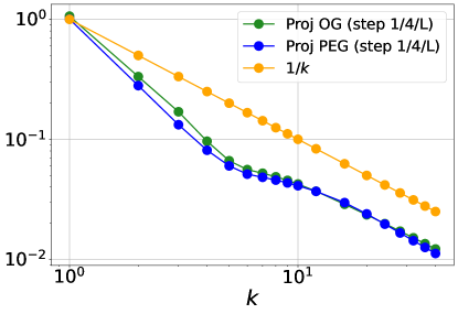
Figure 2: Worst-case ratios $\nicefrac{{\|x^{N}-x^{N-1}\|^{2}}}{{\|x^{0}-x^{*}\|^{2}}}$ (for Proj-PEG) and $\nicefrac{{\|\widetilde{x}^{N}-\widetilde{x}^{N-1}\|^{2}}}{{\|x^{0}-x^{*}\|^{2}}}$ (for Proj-OG) as functions of $N$, computed with PESTO [Taylor et al., 2017b] ($L=1$, $\gamma=\nicefrac{{1}}{{4L}}$).

References

- Abernethy et al. [2019] J. Abernethy, K. A. Lai, and A. Wibisono. Last-iterate convergence rates for min-max optimization. arXiv preprint arXiv:1906.02027, 2019.
- Anagnostides et al. [2022] I. Anagnostides, I. Panageas, G. Farina, and T. Sandholm. On last-iterate convergence beyond zero-sum games. arXiv preprint arXiv:2203.12056, 2022.
- Azizian et al. [2020a] W. Azizian, I. Mitliagkas, S. Lacoste-Julien, and G. Gidel. A tight and unified analysis of gradient-based methods for a whole spectrum of differentiable games. In International Conference on Artificial Intelligence and Statistics, pages 2863–2873. PMLR, 2020a.
- Azizian et al. [2020b] W. Azizian, D. Scieur, I. Mitliagkas, S. Lacoste-Julien, and G. Gidel. Accelerating smooth games by manipulating spectral shapes. In International Conference on Artificial Intelligence and Statistics. PMLR, 2020b.
- Ben-Tal et al. [2009] A. Ben-Tal, L. El Ghaoui, and A. Nemirovski. Robust optimization. Princeton university press, 2009.
- Brown and Sandholm [2019] N. Brown and T. Sandholm. Solving imperfect-information games via discounted regret minimization. In Proceedings of the AAAI Conference on Artificial Intelligence, volume 33, pages 1829–1836, 2019.
- Cai et al. [2022] Y. Cai, A. Oikonomou, and W. Zheng. Tight last-iterate convergence of the extragradient method for constrained monotone variational inequalities. arXiv preprint arXiv:2204.09228 version 1, 2022.
- Daskalakis et al. [2018] C. Daskalakis, A. Ilyas, V. Syrgkanis, and H. Zeng. Training gans with optimism. In International Conference on Learning Representations, 2018.
- De Klerk et al. [2017] E. De Klerk, F. Glineur, and A. B. Taylor. On the worst-case complexity of the gradient method with exact line search for smooth strongly convex functions. Optimization Letters, 11(7):1185–1199, 2017.
- Diakonikolas [2020] J. Diakonikolas. Halpern iteration for near-optimal and parameter-free monotone inclusion and strong solutions to variational inequalities. In Conference on Learning Theory. PMLR, 2020.
- Drori and Teboulle [2014] Y. Drori and M. Teboulle. Performance of first-order methods for smooth convex minimization: a novel approach. Mathematical Programming, 145(1):451–482, 2014.
- Facchinei and Pang [2003] F. Facchinei and J.-S. Pang. Finite-dimensional variational inequalities and complementarity problems. Springer, 2003.
- Farina et al. [2019] G. Farina, C. Kroer, N. Brown, and T. Sandholm. Stable-predictive optimistic counterfactual regret minimization. In International conference on machine learning, pages 1853–1862. PMLR, 2019.
- Gidel et al. [2019a] G. Gidel, H. Berard, P. Vincent, and S. Lacoste-Julien. A variational inequality perspective on generative adversarial nets. In ICLR, 2019a.
- Gidel et al. [2019b] G. Gidel, R. A. Hemmat, M. Pezeshki, R. Le Priol, G. Huang, S. Lacoste-Julien, and I. Mitliagkas. Negative momentum for improved game dynamics. In The 22nd International Conference on Artificial Intelligence and Statistics, pages 1802–1811. PMLR, 2019b.
- Golowich et al. [2020a] N. Golowich, S. Pattathil, and C. Daskalakis. Tight last-iterate convergence rates for no-regret learning in multi-player games. arXiv preprint arXiv:2010.13724, 2020a.
- Golowich et al. [2020b] N. Golowich, S. Pattathil, C. Daskalakis, and A. Ozdaglar. Last iterate is slower than averaged iterate in smooth convex-concave saddle point problems. In Conference on Learning Theory, pages 1758–1784. PMLR, 2020b.
- Goodfellow et al. [2014] I. Goodfellow, J. Pouget-Abadie, M. Mirza, B. Xu, D. Warde-Farley, S. Ozair, A. Courville, and Y. Bengio. Generative adversarial nets. Advances in neural information processing systems, 27, 2014.
- Goodfellow et al. [2015] I. J. Goodfellow, J. Shlens, and C. Szegedy. Explaining and harnessing adversarial examples. ICLR 2015, 2015.
- Gorbunov et al. [2021] E. Gorbunov, N. Loizou, and G. Gidel. Extragradient method: O last-iterate convergence for monotone variational inequalities and connections with cocoercivity. arXiv preprint arXiv:2110.04261, 2021.
- Goujaud et al. [2022] B. Goujaud, C. Moucer, F. Glineur, J. Hendrickx, A. Taylor, and A. Dieuleveut. Pepit: computer-assisted worst-case analyses of first-order optimization methods in python. arXiv preprint arXiv:2201.04040, 2022.
- Halpern [1967] B. Halpern. Fixed points of nonexpanding maps. Bulletin of the American Mathematical Society, 1967.
- Hast et al. [2013] M. Hast, K. J. Åström, B. Bernhardsson, and S. Boyd. Pid design by convex-concave optimization. In 2013 European Control Conference (ECC), pages 4460–4465. IEEE, 2013.
- Henrion et al. [2016] D. Henrion, S. Naldi, and M. S. El Din. Exact algorithms for linear matrix inequalities. SIAM Journal on Optimization, 26(4):2512–2539, 2016.
- Hsieh et al. [2019] Y.-G. Hsieh, F. Iutzeler, J. Malick, and P. Mertikopoulos. On the convergence of single-call stochastic extra-gradient methods. Advances in Neural Information Processing Systems, 32:6938–6948, 2019.
- Korpelevich [1976] G. M. Korpelevich. The extragradient method for finding saddle points and other problems. Matecon, 12:747–756, 1976.
- Lasserre [2001] J. B. Lasserre. Global optimization with polynomials and the problem of moments. SIAM Journal on optimization, 2001.
- Lee and Kim [2021] S. Lee and D. Kim. Fast extra gradient methods for smooth structured nonconvex-nonconcave minimax problems. Advances in Neural Information Processing Systems, 34, 2021.
- Liang and Stokes [2019] T. Liang and J. Stokes. Interaction matters: A note on non-asymptotic local convergence of generative adversarial networks. In The 22nd International Conference on Artificial Intelligence and Statistics, pages 907–915. PMLR, 2019.
- Lofberg [2004] J. Lofberg. Yalmip: A toolbox for modeling and optimization in matlab. In 2004 IEEE international conference on robotics and automation (IEEE Cat. No. 04CH37508), pages 284–289. IEEE, 2004.
- Loizou et al. [2020] N. Loizou, H. Berard, A. Jolicoeur-Martineau, P. Vincent, S. Lacoste-Julien, and I. Mitliagkas. Stochastic hamiltonian gradient methods for smooth games. In International Conference on Machine Learning, pages 6370–6381. PMLR, 2020.
- Madry et al. [2018] A. Madry, A. Makelov, L. Schmidt, D. Tsipras, and A. Vladu. Towards deep learning models resistant to adversarial attacks. ICLR 2018, 2018.
- Mokhtari et al. [2019] A. Mokhtari, A. Ozdaglar, and S. Pattathil. Proximal point approximations achieving a convergence rate of O for smooth convex-concave saddle point problems: Optimistic gradient and extra-gradient methods. arXiv preprint arXiv:1906.01115, 2019.
- Mosek [2010] A. Mosek. The MOSEK optimization software, 2010. URL http://www.mosek.com.
- Nesterov [2000] Y. Nesterov. Squared functional systems and optimization problems. In High performance optimization, pages 405–440. Springer, 2000.
- Nesterov [2007] Y. Nesterov. Dual extrapolation and its applications to solving variational inequalities and related problems. Mathematical Programming, 109(2):319–344, 2007.
- Parrilo [2000] P. A. Parrilo. Structured semidefinite programs and semialgebraic geometry methods in robustness and optimization. California Institute of Technology, 2000.
- Peng et al. [2020] W. Peng, Y.-H. Dai, H. Zhang, and L. Cheng. Training gans with centripetal acceleration. Optimization Methods and Software, 35(5):955–973, 2020.
- Popov [1980] L. D. Popov. A modification of the arrow-hurwicz method for search of saddle points. Mathematical notes of the Academy of Sciences of the USSR, 28(5):845–848, 1980.
- Ryu et al. [2020] E. K. Ryu, A. B. Taylor, C. Bergeling, and P. Giselsson. Operator splitting performance estimation: Tight contraction factors and optimal parameter selection. SIAM Journal on Optimization, 30(3):2251–2271, 2020.
- Shor [1987] N. Z. Shor. An approach to obtaining global extremums in polynomial mathematical programming problems. Cybernetics, 1987.
- Sturm [1999] J. F. Sturm. Using sedumi 1.02, a MATLAB toolbox for optimization over symmetric cones. Optimization Methods and Software, 11(1-4):625–653, 1999. doi: 10.1080/10556789908805766. URL https://doi.org/10.1080/10556789908805766.
- Taylor et al. [2017a] A. B. Taylor, J. M. Hendrickx, and F. Glineur. Exact worst-case performance of first-order methods for composite convex optimization. SIAM Journal on Optimization, 27(3):1283–1313, Jan 2017a. ISSN 1095-7189.
- Taylor et al. [2017b] A. B. Taylor, J. M. Hendrickx, and F. Glineur. Performance estimation toolbox (pesto): automated worst-case analysis of first-order optimization methods. In 2017 IEEE 56th Annual Conference on Decision and Control (CDC), pages 1278–1283. IEEE, 2017b.
- Taylor et al. [2017c] A. B. Taylor, J. M. Hendrickx, and F. Glineur. Smooth strongly convex interpolation and exact worst-case performance of first-order methods. Mathematical Programming, 161(1):307–345, 2017c.
- Tran-Dinh [2022] Q. Tran-Dinh. The connection between nesterov’s accelerated methods and halpern fixed-point iterations. arXiv preprint arXiv:2203.04869, 2022.
- Tran-Dinh and Luo [2021] Q. Tran-Dinh and Y. Luo. Halpern-type accelerated and splitting algorithms for monotone inclusions. arXiv preprint arXiv:2110.08150, 2021.
- Tseng [1995] P. Tseng. On linear convergence of iterative methods for the variational inequality problem. Journal of Computational and Applied Mathematics, 60(1-2):237–252, 1995.
- Yoon and Ryu [2021] T. Yoon and E. K. Ryu. Accelerated algorithms for smooth convex-concave minimax problems with O rate on squared gradient norm. In International Conference on Machine Learning, pages 12098–12109. PMLR, 2021.
- Zhang and Yu [2020] G. Zhang and Y. Yu. Convergence of gradient methods on bilinear zero-sum games. In International Conference on Learning Representations, 2020.