KiT-RT: An extendable framework for radiative transfer and therapy

Abstract.

In this paper we present KiT-RT (Kinetic Transport Solver for Radiation Therapy), an open-source C++ based framework for solving kinetic equations in radiation therapy applications. The aim of this code framework is to provide a collection of classical deterministic solvers for unstructured meshes that allow for easy extendability. Therefore, KiT-RT is a convenient base to test new numerical methods in various applications and compare them against conventional solvers. The implementation includes spherical-harmonics, minimal entropy, neural minimal entropy and discrete ordinates methods. Solution characteristics and efficiency are presented through several test cases ranging from radiation transport to electron radiation therapy. Due to the variety of included numerical methods and easy extendability, the presented open source code is attractive for both developers, who want a basis to build their own numerical solvers and users or application engineers, who want to gain experimental insights without directly interfering with the codebase.

1. Introduction

Personalized medicine in radiation oncology has been an important research topic in the last decades. To allow for accurate, reliable and efficient treatment planning tailored towards individual patient needs, there is a growing desire to undertake direct numerical simulation for radiation therapy. High-fidelity numerical solutions enable quantitative estimation of the dose received by the tumor as well as the surrounding tissue, while allowing for an automated generation of optimal treatment plans. Besides the aim to ensure sufficient accuracy, such simulations are required to run on limited computational resources such as workstation PCs.

Traditional methods to predict dose distributions in radiation oncology largely rely on simplified models, such as pencil beam models based on the Fermi-Eyges theory (Eyges, 1948). While such models are computationally efficient, they often lack the required accuracy, especially in cases including air cavities or other inhomogeneities (Hogstrom et al., 1981; Krieger and Sauer, 2005). On the other hand, Monte Carlo (MC) algorithms, which simulate individual interacting particles, achieve a satisfactory accuracy (Andreo, 1991). However, despite ongoing research to accelerate MC methods, their high computational costs currently renders them impractical for clinical usage (Fippel and Soukup, 2004; Jia et al., 2012). To obtain a computationally feasible model with comparable accuracy, radiation particles are described on a mesoscopic level through the deterministic linear Boltzmann equation (Börgers, 1998; Tervo et al., 1999; Tervo and Kolmonen, 2002; Tervo et al., 2008). An efficient and accurate numerical approximation to the linear Boltzmann equation can be achieved through the construction of grid-based macroscopic approximations (Duclous et al., 2010; Vassiliev et al., 2010, 2008; Gifford et al., 2006). Variants of grid based methods for radiation therapy can be found in for example (Hensel et al., 2006; Barnard et al., 2012; Huang, 2015; Olbrant and Frank, 2010; Kuepper, 2016; Kusch and Stammer, 2021).

The available grid-based methods employ various macroscopic approximations to the linear Boltzmann equation which all exhibit certain advantages and shortcomings.

In (Duclous et al., 2010), the modal entropy method called $M_{N}$ is used as a macroscopic model. This method preserves positivity of particle distributions while yielding accurate results with little spurious oscillations. However, the need to solve a possibly ill-posed optimization problem in every spatial cell and time step results in increased computational costs. While analytic solutions to the optimization problems are available at small truncation order, they cannot capture all physical effects accurately. Further approaches aim at mitigating the challenge of the problems ill-condition by regularization  (Alldredge et al., 2018) or reducing the associated computational costs, e.g. using neural networks  (Schotthöfer et al., 2022).

In (Olbrant and Frank, 2010) the use of computationally cheap nodal discretizations, known as the $S_{N}$ method has been proposed. In this case, the solution remains positive and it is shown that the expensive scattering terms can be approximated efficiently with a Fokker-Planck approximation. Furthermore, the solution can exhibit non-physical artifacts, known as ray-effects (Lathrop, 1968; Mathews, 1999; Morel et al., 2003), which reduce the approximation quality. While methods to mitigate ray-effects exist, see e.g. (Camminady et al., 2019; Frank et al., 2020; Abu-Shumays, 2001; Lathrop, 1971; Tencer, 2016), they commonly require picking problem-dependent tuning parameters.

In (Kuepper, 2016), the modal $P_{N}$ method has been employed to derive a macroscopic model for radiation treatment planning. While it does not preserve positivity of the solution and can potentially yield oscillatory approximations, it allows for an efficient numerical treatment of scattering terms. In (Kusch and Stammer, 2021) a combination of $S_{N}$ and $P_{N}$ methods which reduces computational costs through a dynamical low rank approximation (Koch and Lubich, 2007) has been proposed. The efficiency of this method relies on the ability to describe the solution through a low-rank function.

The variety of different methods allows for individual method choices tailored to different settings. The comparability of different methods in a uniform framework is not only interesting for clinical usage, but also for future research in computational radiation therapy. Our aim of the open-source C++ Kinetic Transport for radiation therapy (KiT-RT) framework is therefore to provide a collection of available deterministic methods. Special focus is put on extendability by the use of polymorphism to simplify the implementation of novel solution methods. The methods provided by our framework are optimized for an application on workstation PCs. This meets the typical requirements in radiation therapy applications: For clinical usage the computational resources are often limited and the time between recording the CT image and the actual treatment must not exceed a certain time period. Hence, radiation therapy codes that are applicable for clinical use should run efficiently on workstation PCs. Moreover, conventional codes often require structured grids (Seibold and Frank, 2014; Wieser et al., 2017; Perl et al., 2012; Garrett and Hauck, 2013; Kristopher Garrett et al., 2015), leading to inaccurate representations of structures on CT images. While accuracy in practice is also limited by the CT density values which are given on a structured grid, these are often downsampled to a lower resolution for dose computations. Further, a recomputation of the CT values for unstructured grids is feasible if it improves the quality of dose computations. Therefore, our framework provides functionalities for both unstructured meshes which preserve organ outlines on CT images, as well as standard rectangular grids.

This paper aims at presenting the developed framework and its functionality while providing the necessary mathematical and physical background on principles the software is based on. In Section 2 we provide the underlying physical model as well as its reformulation as a time-dependent partial differential equation. Section 3 discusses different macroscopic models as well as advantages and disadvantages of the individual underlying directional discretizations. Sections 4 and 5 focus on the used discretizations and software architecture, respectively. Lastly, we validate our implementations and analyse their performance for different test cases in Section 7.

2. Physical model

Let us recap the main physical model that is used for computational radiotherapy treatment planning. The main goal is to compute the radiation dose distribution

(1) $$D(\mathbf{x})=\frac{1}{\rho(\mathbf{x})}\int_{0}^{\infty}\int_{\mathbb{S}^{2}}S(E,\mathbf{x})\psi(E,\mathbf{x},\mathbf{\Omega})\;\mathrm{d}\mathbf{\Omega}\;\mathrm{d}E\;,$$

that results from a given treatment plan. Here, $E\in\mathbb{R}_{+}$ is the energy, $\mathbf{x}\in\mathbf{X}\subset\mathbb{R}^{3}$ denotes the spatial domain, and $\mathbf{\Omega}\in\mathbb{S}^{2}$ is the flight direction of particles. Moreover, $\psi:\mathbb{R}_{+}\times\mathbb{R}^{3}\times\mathbb{S}^{2}\rightarrow\mathbb{R}$ denotes the radiation flux density and $\rho:\mathbb{R}^{3}\rightarrow\mathbb{R}$ is the patient tissue density. The stopping power $S:\mathbb{R}_{+}\times\mathbb{R}^{3}\rightarrow\mathbb{R}$ models the continuous energy loss of particles due to scattering with tissue and is defined as

(2) $$S(E,\mathbf{x})=\int_{0}^{\infty}E^{\prime}\int_{-1}^{1}\Sigma(E,E^{\prime},\mathbf{x},\mu)\;\mathrm{d}\mu\;\mathrm{d}E^{\prime}$$

with the scattering cross section $\Sigma:\mathbb{R}_{+}\times\mathbb{R}_{+}\times\mathbb{R}^{3}\times[-1,1]\rightarrow\mathbb{R}$. The radiation flux density, which describes the probability of finding a particle at a certain region in phase space, can be computed from the continuous slowing down (CSD) approximation (Larsen et al., 1997) of the energy dependent linear Boltzmann equation

(3) $$-\partial_{E}\left(S(E,\mathbf{x})\psi(E,\mathbf{x},\mathbf{\Omega})\right)+\mathbf{\Omega}\cdot\nabla_{x}\psi(E,\mathbf{x},\mathbf{\Omega})+\Sigma_{t}(E,\mathbf{x})\psi(E,\mathbf{x},\mathbf{\Omega})$$

$$=\int_{\mathbb{S}^{2}}\Sigma_{s}(E,\mathbf{x},\mathbf{\Omega}\cdot\mathbf{\Omega}^{\prime})\psi(E,\mathbf{x},\mathbf{\Omega}^{\prime})\;\mathrm{d}\mathbf{\Omega}^{\prime}\;.$$

This model assumes a continuous energy loss of particles traveling through a background material, which is modeled using the stopping power $S$. The scattering cross section $\Sigma_{s}(E,\mathbf{x},\mathbf{\Omega}\cdot\mathbf{\Omega}^{\prime})$ denotes the probability of particles at position $\mathbf{x}$ with energy $E$ changing their flight direction from $\mathbf{\Omega}^{\prime}$ to $\mathbf{\Omega}$ due to a collision with the patient tissue. The total cross section $\Sigma_{t}$ is given by

(4) $$\Sigma_{t}(E,\mathbf{x})=\Sigma_{s,0}(E,\mathbf{x})=2\pi\int_{-1}^{1}\Sigma_{s}(E,\mathbf{x},\mu)\;\mathrm{d}\mu\;.$$

To simplify the evaluation of material properties, we follow the common assumption that all materials are water-equivalent and differ only in density (e.g. Woo and Cunningham, 1990; Olbrant and Frank, 2010; Kuepper, 2016), i.e.,

(5) $$S(E,\mathbf{x})=S^{H_{2}O}(E)\rho(\mathbf{x}),$$

$$\Sigma_{t}(E,\mathbf{x})=\Sigma_{t}^{H_{2}O}(E)\rho(\mathbf{x}),$$

$$\Sigma_{s}(E,\mathbf{x},\mathbf{\Omega}\cdot\mathbf{\Omega}^{\prime})=\Sigma_{s}^{H_{2}O}(E,\mathbf{\Omega}\cdot\mathbf{\Omega}^{\prime})\rho(\mathbf{x})\;,$$

where we leave out the superscript $H_{2}O$ in the following. Cross-sections for water are taken from the ICRU database (Grégoire and Mackie, 2011). Having defined the prerequisites of our physical model, we can focus on bringing it into a form that allows for computing numerical approximations efficiently. It turns out that the energy variable in (3) can be treated as a pseudo-time, which facilitates solving the CSD equation. For a given maximal energy $E_{\mathrm{max}}$ let us define the transformed energy as

(6) $$\widetilde{E}(E):=\int_{0}^{E_{\mathrm{max}}}\frac{1}{S(E^{\prime})}\;\mathrm{d}E^{\prime}-\int_{0}^{E}\frac{1}{S(E^{\prime})}\;\mathrm{d}E^{\prime}$$

and the transformed particle density as

(7) $$\widetilde{\psi}(\widetilde{E},\mathbf{x},\mathbf{\Omega}):=S(E)\rho(\mathbf{x})\psi(E(\widetilde{E}),\mathbf{x},\mathbf{\Omega})\;.$$

Then, multiplying (3) with $S(E)$ and plugging in the defined transformation gives

(8) $$\partial_{\widetilde{E}}\widetilde{\psi}(\widetilde{E},\mathbf{x},\mathbf{\Omega})+\mathbf{\Omega}\cdot\nabla_{x}\frac{\widetilde{\psi}(\widetilde{E},\mathbf{x},\mathbf{\Omega})}{\rho(\mathbf{x})}+\widetilde{\Sigma}_{t}(\widetilde{E})\widetilde{\psi}(\widetilde{E},\mathbf{x},\mathbf{\Omega})=\int_{\mathbb{S}^{2}}\widetilde{\Sigma}_{s}(\widetilde{E},\mathbf{\Omega}\cdot\mathbf{\Omega}^{\prime})\widetilde{\psi}(\widetilde{E},\mathbf{x},\mathbf{\Omega}^{\prime})\;\mathrm{d}\mathbf{\Omega}^{\prime}\;,$$

where we define $\widetilde{\Sigma}_{t}(\widetilde{E}):=\Sigma_{t}(E(\widetilde{E}))$ and $\widetilde{\Sigma}_{s}(\widetilde{E},\mathbf{\Omega}\cdot\mathbf{\Omega}^{\prime}):=\Sigma_{s}(E(\widetilde{E}),\mathbf{\Omega}\cdot\mathbf{\Omega}^{\prime})$. Dropping the tilde notation and treating $\widetilde{E}$ as a pseudo-time $t$ gives a slightly modified version of the classical linear Boltzmann equation

(9) $$\partial_{t}\psi(t,\mathbf{x},\mathbf{\Omega})+ \mathbf{\Omega}\cdot\nabla_{x}\frac{\psi(t,\mathbf{x},\mathbf{\Omega})}{\rho(\mathbf{x})}+\Sigma_{t}(t)\psi(t,\mathbf{x},\mathbf{\Omega})=\int_{\mathbb{S}^{2}}\Sigma_{s}(t,\mathbf{\Omega}\cdot\mathbf{\Omega}^{\prime})\psi(t,\mathbf{x},\mathbf{\Omega}^{\prime})\;\mathrm{d}\mathbf{\Omega}^{\prime}$$

$$\psi(t=0,\mathbf{x},\mathbf{\Omega})=S(E_{\text{max}})\rho(\mathbf{x})\psi(E_{\text{max}},\mathbf{x},\mathbf{\Omega})\;.$$

Hence, the CSD equation can be treated numerically with classical closure methods and space-time discretizations. Let us first discuss methods to discretize the directional domain, yielding macroscopic evolution equations.

3. Macroscopic models

This section discusses macroscopic models to (9). These models are derived from nodal and modal discretizations of the directional domain.

3.1. Modal discretizations

Modal discretizations of (9) can be interpreted as a closure problem (Levermore, 1997, 1996). To present the derivation of different closures, we first formulate the moment equations which are not closed. Second, we close these equations with the $P_{N}$ closure and third, we derive the $M_{N}$ closure.

Moment equations

Let us derive an evolution equation to describe the moments of the radiation flux with respect to the real-valued spherical harmonics basis functions. These are defined as the real parts of the spherical harmonics

$$Y_{\ell}^{k}(\mathbf{\Omega})=\sqrt{\frac{2\ell+1}{4\pi}\frac{(\ell-k)!}{(\ell+k)!}}\ e^{ik\varphi}P_{\ell}^{k}(\mu)\;,$$

where $P_{\ell}^{k}$ are the associated Legendre polynomials. Then, the real spherical harmonics are given as

$$m_{\ell}^{k}(\mathbf{\Omega})=\begin{cases}\frac{(-1)^{k}}{\sqrt{2}}\left(Y_{\ell}^{k}(\mathbf{\Omega})+(-1)^{k}Y_{\ell}^{-k}(\mathbf{\Omega})\right),&k>0\;,\\ Y_{\ell}^{0}(\mathbf{\Omega})&k=0\;,\\ -\frac{(-1)^{k}i}{\sqrt{2}}\left(Y_{\ell}^{-k}(\mathbf{\Omega})-(-1)^{k}Y_{\ell}^{k}(\mathbf{\Omega})\right),&k<0\;,\end{cases}$$

where $i$ is the imaginary unit. Collecting all basis functions up to degree $N$ in a vector

$$\mathbf{m}=\left(m_{0}^{0},m_{1}^{-1},m_{1}^{0},m_{1}^{1},\cdots,m_{N}^{N}\right)^{T}\in\mathbb{R}^{(N+1)^{2}}$$

yields the so-called moments

$$u_{\ell}^{k}(t,\mathbf{x}):=\int_{\mathbb{S}^{2}}\psi(t,\mathbf{x},\mathbf{\Omega})m_{\ell}^{k}(\mathbf{\Omega})\;\mathrm{d}\mathbf{\Omega}\;.$$

Evolution equations for the moments can be derived by testing (9) against $\mathbf{m}_{\ell}=(m_{\ell}^{-\ell},\cdots,m_{\ell}^{\ell})$, which gives

$$\partial_{t}\mathbf{u}_{\ell}(t,\mathbf{x})+ \nabla_{x}\cdot\int_{\mathbb{S}^{2}}\mathbf{\Omega}\mathbf{m}_{\ell}(\mathbf{\Omega})\frac{\psi(t,\mathbf{x},\mathbf{\Omega})}{\rho(\mathbf{x})}\;\mathrm{d}\mathbf{\Omega}+\Sigma_{t}(t)\mathbf{u}_{\ell}(t,\mathbf{x})$$

(10) $$=\int_{\mathbb{S}^{2}}\int_{\mathbb{S}^{2}}\mathbf{m}_{\ell}(\mathbf{\Omega})\Sigma_{s}(t,\mathbf{\Omega}\cdot\mathbf{\Omega}^{\prime})\psi(t,\mathbf{x},\mathbf{\Omega}^{\prime})\;\mathrm{d}\mathbf{\Omega}^{\prime}\;\mathrm{d}\mathbf{\Omega}\;.$$

To rewrite this equation, we use the spherical harmonics recursion relation

$$\Omega_{i}\mathbf{m}_{\ell}=\mathbf{a}_{\ell}^{i}\mathbf{m}_{\ell-1}+\mathbf{a}_{\ell+1}^{i}\mathbf{m}_{\ell+1}\enskip\text{ with }\mathbf{a}_{\ell}^{i}\in\mathbb{R}^{(2\ell-1)\times(2\ell+1)}$$

as well as the fact that there exists a diagonal matrix $\bm{\Sigma}_{\ell}(t)$ with entries $\Sigma_{\ell,kk}=\Sigma_{\ell}^{k}:=2\pi\int_{[-1,1]}P_{\ell}(\mu)\Sigma_{s}(t,\mu)\;\mathrm{d}\mu$ such that

$$\int_{\mathbb{S}^{2}}\int_{\mathbb{S}^{2}}\mathbf{m}_{\ell}(\mathbf{\Omega})\Sigma_{s}(t,\mathbf{\Omega}\cdot\mathbf{\Omega}^{\prime})\psi(t,\mathbf{x},\mathbf{\Omega}^{\prime})\;\mathrm{d}\mathbf{\Omega}^{\prime}d\mathbf{\Omega}=\bm{\Sigma}_{\ell}(t)\mathbf{u}_{\ell}(t,\mathbf{x})\;.$$

Then, the moment equations at degree $\ell$ become

$$\partial_{t}\mathbf{u}_{\ell}(t,\mathbf{x})+ \sum_{i=1}^{3}\partial_{x_{i}}\left(\mathbf{a}_{\ell}^{i}\mathbf{u}_{\ell-1}(t,\mathbf{x})+\mathbf{a}_{\ell+1}^{i}\mathbf{u}_{\ell+1}(t,\mathbf{x})\right)/\rho(\mathbf{x})+\Sigma_{t}(t)\mathbf{u}_{\ell}(t,\mathbf{x})$$

(11) $$=\bm{\Sigma}_{\ell}(t)\mathbf{u}_{\ell}(t,\mathbf{x})\;.$$

Note that the equations for degree $\ell$ depend on the moments of degree $\ell+1$. Hence, to obtain a closed system of moments up to a fixed degree $N$, we need to define a closure relation

(12) $$\mathbf{u}_{N+1}(t,\mathbf{x})\simeq\mathcal{U}(\mathbf{u}_{0}(t,\mathbf{x}),\cdots,\mathbf{u}_{N}(t,\mathbf{x}))\;.$$

$P_{N}$ closure

The most commonly used closure is the $P_{N}$ closure which leads to the spherical harmonics ($P_{N}$) method (Case and Zweifel, 1967). It expands the solution by spherical harmonics, i.e.,

(13) $$\psi(t,\mathbf{x},\mathbf{\Omega})\approx\psi_{\mathrm{P}_{N}}(t,\mathbf{x},\mathbf{\Omega}):=\mathbf{u}(t,\mathbf{x})^{T}\mathbf{m}(\mathbf{\Omega})\;,$$

where $\mathbf{u}\in\mathbb{R}^{(N+1)^{2}}$ collects all moments according to $\mathbf{u}=\left(u_{0}^{0},u_{1}^{-1},u_{1}^{0},u_{1}^{1},\cdots,u_{N}^{N}\right)^{T}\in\mathbb{R}^{(N+1)^{2}}$. Hence, the $P_{N}$ closure is simply given as $\mathcal{U}_{\mathrm{P}_{N}}\equiv\mathbf{0}$. In this case, the moment equations read

$$\partial_{t}\mathbf{u}(t,\mathbf{x})=-\mathbf{A}\cdot\nabla_{\mathbf{x}}\frac{\mathbf{u}(t,\mathbf{x})}{\rho(\mathbf{x})}-\Sigma_{t}(t)\mathbf{u}(t,\mathbf{x})+\bm{\Sigma}\mathbf{u}(t,\mathbf{x}),\;$$

where $\mathbf{A}\cdot\nabla_{\mathbf{x}}:=\mathbf{A}_{1}\partial_{x}+\mathbf{A}_{2}\partial_{y}+\mathbf{A}_{3}\partial_{z}$ with $\mathbf{A}_{i}:=\int_{\mathbb{S}^{2}}\mathbf{m}\mathbf{m}^{T}\Omega_{i}\;\mathrm{d}\mathbf{\Omega}$ and $\bm{\Sigma}=\mathrm{diag}\left(\Sigma_{0}^{0},\Sigma_{1}^{-1},\Sigma_{1}^{0},\Sigma_{1}^{1},\cdots,\Sigma_{N}^{N}\right)$. While $P_{N}$ is a computationally efficient method (especially for scattering terms), it does not preserve positivity of the radiation flux approximation and can lead to spurious oscillations. A closure which mitigates oscillations and preserves positivity at significantly increased computational costs is the $M_{N}$ closure.

$M_{N}$ closure

The $M_{N}$ closure (Levermore, 1996, 1997) employs the principle of minimal mathematical, i.e., maximal physical entropy to close the moment system. To this end, we define the twice differentiable, strictly convex kinetic entropy density $\eta:\mathbb{R}_{+}\rightarrow\mathbb{R}$. Different, problem specific entropy densities can be defined, e.g. the Maxwell-Boltzmann entropy $\eta(g)=g\log(g)-g$, or a quadratic entropy $\eta(g)=g^{2}$, which recovers the $P_{N}$ method. Thus, one can close the system by choosing the reconstructed radiation flux density $\psi_{\mathbf{u}}$ out of the set of all possible functions

(14) $$F_{\mathbf{m}}=\left\{g(t,x,\mathbf{\Omega})>0:u=\int_{\mathbb{S}^{2}}{\mathbf{m}g}\;\mathrm{d}\mathbf{\Omega}<\infty\right\},$$

that fulfill the moment condition $\mathbf{u}(t,\mathbf{x})=\left<\mathbf{m}g\right>$ as the one with minimal entropy. The modal basis $\mathbf{m}$ can be chosen arbitrarily. Common choices consist of spherical harmonics or other polynomial basis functions. The minimal entropy closure can be formulated as a constrained optimization problem for a given vector of moments $\mathbf{u}$,

(15) $$\min_{g\in F_{\mathbf{m}}}\int_{\mathbb{S}^{2}}\eta(g)\;\mathrm{d}\mathbf{\Omega}\quad\text{ s.t. }\mathbf{u}=\int_{\mathbb{S}^{2}}{\mathbf{m}g}\;\mathrm{d}\mathbf{\Omega}.$$

The minimal value of the objective function is denoted by $h(u)=\left<\eta(\psi_{\mathbf{u}})\right>$ and describes the systems minimal entropy depending on time and space. $\psi_{\mathbf{u}}$ is the minimizer of Eq. (15), which we use to close the moment system

(16) $$\partial_{t}\mathbf{u}_{\ell}(t,\mathbf{x})+ \nabla_{x}\cdot\int_{\mathbb{S}^{2}}\mathbf{\Omega}\mathbf{m}_{\ell}(\mathbf{\Omega})\frac{\psi_{u}(t,\mathbf{x},\mathbf{\Omega})}{\rho(\mathbf{x})}\;\mathrm{d}\mathbf{\Omega}+\Sigma_{t}(t)\mathbf{u}_{\ell}(t,\mathbf{x})=\Sigma_{\ell}\mathbf{u}_{\ell}(t,\mathbf{x});.$$

The minimal entropy method preserves important properties of the underlying equation (Levermore, 1997; Alldredge et al., 2018), i.e., positivity of the solution, hyperbolicity of the moment system, dissipation of mathematical entropy and the H-Theorem. The minimal entropy closed moment system is invariant under Galilean transforms. Lastly, if collision invariants of the Boltzmann equations are used as modal basis functions, then the moment system yields a local conservation law.
The set of all moments corresponding to a radiation flux density $\psi_{\mathbf{u}}>0$ is called the realizable set

(17) $$\mathcal{R}=\left\{\mathbf{u}:\int_{\mathbb{S}^{2}}{\mathbf{m}g}\;\mathrm{d}\mathbf{\Omega}=\mathbf{u},\,g\in F_{\mathbf{m}}\right\}.$$

Outside $\mathcal{R}$ the minimal entropy closure problem has no solution. At the boundary $\partial\mathcal{R}$, the optimization problem becomes singular and $\psi_{\mathbf{u}}$ consists of a linear combination of dirac distributions. Near $\partial\mathcal{R}$ the entropy closure becomes ill conditioned and thus, a numerical optimizer requires a large amount of iterations to compute a solution.

To mitigate this issue, a regularized version of the entropy closure problem has been proposed by (Alldredge et al., 2018),

(18) $$\inf_{g\in F_{\mathbf{m}}}\int_{\mathbb{S}^{2}}\eta(g)\;\mathrm{d}\mathbf{\Omega}+\frac{1}{2\gamma}\left\lVert\int_{\mathbb{S}^{2}}{\mathbf{m}g}\;\mathrm{d}\mathbf{\Omega}-\mathbf{u}\right\rVert^{2}_{2},$$

where $\gamma$ is the regularization parameter. Generally, moments of the regularized reconstructed radiation flux density $\int_{\mathbb{S}^{2}}\mathbf{m}\psi_{\mathbf{u}}\;\mathrm{d}\mathbf{\Omega}$ deviate from the non-regularized moments. For $\gamma\rightarrow 0$, we recover the original entropy closure of Eq. (15) and the moments coincide again. The regularized entropy closure is solvable for any $\mathbf{u}\in\mathbb{R}^{(N+1)^{2}}$ and preserves all structural properties of the non-regularized entropy closure (Alldredge et al., 2018). One can also choose to regularize only parts of the entropy closure, e.g. to preserve moments of specific interest. Then the partially regularized entropy closure reads

(19) $$\inf_{g\in F_{m}}\int_{\mathbb{S}^{2}}\eta(g)\;\mathrm{d}\mathbf{\Omega}+\frac{1}{2\gamma}\left\lVert\int_{\mathbb{S}^{2}}{\mathbf{m}^{r}g}\;\mathrm{d}\mathbf{\Omega}-u^{r}\right\rVert^{2}_{2}\quad\text{ s.t. }\mathbf{u}^{nr}=\int_{\mathbb{S}^{2}}{\mathbf{m}^{nr}g}\;\mathrm{d}\mathbf{\Omega},$$

where $\mathbf{u}^{nr}$ denotes non-regularized moment elements and $\mathbf{u}^{r}$ denotes regularized elements of the moment vector.
Recently, structure preserving deep neural networks have been successfully employed to approximate the entropy closure (Schotthöfer et al., 2022) to accelerate the $M_{N}$ method. The authors leverage convexity of the optimization problem and use corresponding input convex neural networks (Amos et al., 2016) to preserve structural properties of the closure in the neural network based approximation.

3.2. Nodal discretizations

The $S_{N}$ method (Lewis and Miller, 1984) employs a nodal discretization for the directional domain. To facilitate the computation of integral terms that arise due to scattering, the nodal point sets are commonly chosen according to a quadrature rule. In the application case of radiative transport, the directional domain is assumed to be the unit sphere $\mathbb{S}^{2}\subset\mathbb{R}^{3}$, thus a suitable parametrization is given by spherical coordinates

(20) $$\mathbb{S}^{2}=\left\{\begin{pmatrix}\sqrt{1-\mu^{2}}\sin(\varphi)\\ \sqrt{1-\mu^{2}}\cos(\varphi)\\ \mu\end{pmatrix}:\mu\in\left[-1,1\right],\,\varphi\in\left[0,2\pi\right)\right\}.$$

Note, that we can allow different particle velocities by scaling the unit sphere with a given maximum velocity. The implementation assumes a slab geometry setting, i.e., lower dimensional velocity spaces are described by a projection of $\mathbb{S}^{2}$ onto $\mathbb{R}^{2}$ and $\mathbb{R}$, respectively. Thus, the parametrization of the two-dimensional slab geometry is given by

(21) $$P_{\mathbb{R}^{2}}(\mathbb{S}^{2})=\left\{\begin{pmatrix}\sqrt{1-\mu^{2}}\sin(\varphi)\\ \sqrt{1-\mu^{2}}\cos(\varphi)\end{pmatrix}:\mu\in\left[-1,1\right],\,\varphi\in\left[0,2\pi\right)\right\}$$

and the one dimensional case is described by

(22) $$P_{\mathbb{R}}(\mathbb{S}^{2})=\left\{\mu:\mu\in\left[-1,1\right]\right\}$$

Hence the task is to derive a quadrature formula for the direction of travel. The perhaps most common approach is the product quadrature rule. Here. a Gauss quadrature is used for $\mu$ and equally weighted and spaced points for $\varphi$, i.e., when using $N_{q}$ points, we have

(23) $$\varphi_{i}=i\Delta\varphi\quad\text{for}\quad i=1,\ldots,N_{q}\quad\text{and}\quad\Delta\varphi=\frac{2\pi}{N_{q}}\;.$$

If the Gauss quadrature for $\mu$ uses $N_{q}$ points, then we obtain a total of $Q=N_{q}^{2}$ possible directions. Denoting the Gauss weights as $w^{G}_{k}$ with $k=1,\cdots,N_{q}$, we obtain the product quadrature weights

$$w_{k\cdot N_{q}+\ell}=\frac{2\pi w^{G}_{k}}{N_{q}}$$

and points

(24) $$\mathbf{\Omega}_{k\cdot N_{q}+\ell}=\begin{pmatrix}\sqrt{1-\mu_{k}^{2}}\sin(\varphi_{\ell})\\ \sqrt{1-\mu_{k}^{2}}\cos(\varphi_{\ell})\end{pmatrix}\;.$$

Other implemented quadrature methods include spherical Monte Carlo, Levelsymmetric (Longoni, 2004), LEBEDEV (Marchuk and Lebedev, 1986) and LDFESA (Jarrel and Adams, 2011). A comparison of different quadrature sets and their approximation behaviour for $S_{N}$ methods can be found in (Camminady et al., 2021).

The evolution equations for $\psi_{q}(t,\mathbf{x}):=\psi(t,\mathbf{x},\mathbf{\Omega}_{q})$ are then given by

(25) $$\partial_{t}\psi_{q}(t,\mathbf{x})+ \mathbf{\Omega}_{q}\cdot\nabla_{x}\frac{\psi_{q}(t,\mathbf{x})}{\rho(\mathbf{x})}+\Sigma_{t}(t)\psi_{q}(t,\mathbf{x})=\sum_{p=1}^{Q}w_{p}\Sigma_{s}(t,\mathbf{\Omega}_{q}\cdot\mathbf{\Omega}_{p})\psi_{p}(t,\mathbf{x})\;.$$

A main disadvantage of $S_{N}$ methods are so called ray-effects (Lathrop, 1968; Morel et al., 2003; Mathews, 1999), which are spurious artifacts that stem from the limited number of directions in which particles can travel. Moreover, radiation therapy applications exhibit forward-peaked scattering, which cannot be well-captured by classical quadrature rules.

To allow for moderate computational costs when computing scattering terms and to efficiently treat forward-peaked scattering, we transform the nodal solution to a modal description and apply the more efficient $P_{N}$ methodology for scattering terms. For this, we define a truncation order $N$ and construct the matrices $\mathbf{O}\in\mathbb{R}^{Q\times(N+1)^{2}}$ which maps the modal onto its nodal representation and $\mathbf{M}\in\mathbb{R}^{(N+1)^{2}\times Q}$ which maps the nodal onto its modal representation. Such matrices can be constructed by

$$\mathbf{O}=\left(\mathbf{m}(\Omega_{k})\right)_{k=1}^{Q}\,,\text{ and }\enskip\mathbf{M}=\left(w_{k}\mathbf{m}(\Omega_{k})\right)_{k=1}^{Q}.$$

In this case, we can replace the scattering term on the right-hand side of (25) by its $P_{N}$ counterpart. Collecting the nodal solution in the vector $\bm{\psi}$ then gives

(26) $$\partial_{t}\bm{\psi}(t,\mathbf{x})+ \mathbf{\Omega}_{q}\cdot\nabla_{x}\frac{\bm{\psi}(t,\mathbf{x})}{\rho(\mathbf{x})}+\Sigma_{t}(t)\bm{\psi}(t,\mathbf{x})=\mathbf{O}\bm{\Sigma}\mathbf{M}\bm{\psi}\;.$$

4. Discretization methods

4.1. Spatial Discretization

The KiT-RT framework is based on unstructured, cell-centered grids as spatial discretization. In the following, we restrict ourselves to a two-dimensional spatial grid, however, the notations are straight forwardly extended to three or one spatial dimensions. A unstructured grid $\tilde{\mathbf{X}}=\left\{\mathbf{X}_{i}\right\}_{i\in I}$ is a partition of a bounded spatial domain $\mathbf{X}\subset\mathbb{R}^{d}$. A grid cell $\mathbf{X}_{i}$ holds information about the coordinates of its centroid $\mathbf{x}_{i}$, its measure $A_{i}$, the indices of its boundary vertices, indices of its neighbor cells $N(i)$ and cell faces. The information of the cell faces is encoded in the unit-normal vector of the face dividing cell $i$ and its neighbor $j\in N(i)$, multiplied with the measure of the face and is denoted by $\mathbf{n}_{i,j}$. The grids used in this work are either triangular or quadrilateral, unstructured grids in two spatial dimensions.

4.2. Finite volume methods

The nodal and modal methods are different approaches to discretize the velocity space of the Boltzmann equation, however all of them result in a system of transport equations, that can be solved using a finite volume scheme. Thus, we first describe a method agnostic finite volume scheme and afterwards point out the differences of the $S_{N}$, $P_{N}$ and $M_{N}$ based implementations. We denote the temporal variable by $t$, however the results hold for energy interpreted as pseudo-time as well. Let $\mathbf{g}(t,\mathbf{x})\in\mathbb{R}^{m}$ be the vector of conserved variables of a system of transport equations

(27) $$\partial_{t}\mathbf{g}(t,\mathbf{x})+\nabla_{\mathbf{x}}\cdot\mathbf{F}(\mathbf{g}(t,\mathbf{x}))=\mathbf{R}(t,\mathbf{x},\mathbf{g}(t,\mathbf{x})),\qquad\mathbf{x}\in\mathbf{X},\,t\in[0,t_{f})$$

where $\mathbf{F}$ is the general flux function describing the solution transport, and $\mathbf{R}$ is a general right hand side, containing velocity discretizations of collision terms, sources and absorption terms. The main discretization strategy is to divide the spatial domain into an unstructured grid with $N_{x}$ cells and the time domain into $N_{t}$ discrete values $0=t_{0}<\dots<t_{N_{t}-1}$. We consider the solution as an average over one space-time cell

(28) $$\mathbf{g}_{i}^{n}=\frac{1}{A_{i}}\int_{\mathbf{X}_{i}}\mathbf{g}\;\mathrm{d}\mathbf{x}$$

and average Eq. (27) over one space-time cell

(29) $$\begin{aligned} \frac{1}{\Delta tA_{i}}\int_{\mathbf{X}_{i}}\int_{t_{n}}^{t_{n+1}}\partial_{t}\mathbf{g}(t,\mathbf{x})\;\mathrm{d}t\;\mathrm{d}\mathbf{x}&+\\ \frac{1}{\Delta tA_{i}}\int_{\mathbf{X}_{i}}\int_{t_{n}}^{t_{n+1}}\nabla_{\mathbf{x}}\cdot F(\mathbf{g}(t,\mathbf{x}))\;\mathrm{d}t\;\mathrm{d}\mathbf{x}&=\frac{1}{\Delta tA_{i}}\int_{\mathbf{X}_{i}}\int_{t_{n}}^{t_{n+1}}R(t,\mathbf{x},\mathbf{g}(t,\mathbf{x}))\;\mathrm{d}t\;\mathrm{d}\mathbf{x},\end{aligned}$$

where $\Delta t=t_{n+1}-t_{n}$. Solving the integrals using the Gauss theorem for the advection term and an explicit Euler scheme for the time derivative yields

(30) $$\begin{aligned} \frac{1}{\Delta t}\left(\mathbf{g}_{i}^{n+1}-\mathbf{g}_{i}^{n}\right)&+\\ \frac{1}{\Delta tA_{i}}\int_{t_{n}}^{t_{n+1}}\sum_{j\in N(i)}F(\mathbf{g}(t,x_{i,j}))\cdot\mathbf{n}_{i,j}\;\mathrm{d}t&=\frac{1}{\Delta t}\int_{t_{n}}^{t_{n+1}}R(t,\mathbf{x},\mathbf{g}(t,x_{i}))\;\mathrm{d}t,\end{aligned}$$

where $g(t,x_{i})$ is the conserved variable evaluated at cell $i$ and $g(t,x_{i,j})$ is the conserved variable evaluated at the interface between cell $i$ and its neighbor $j$. To compute the actual value of $\mathbf{g}_{j}^{n+1}$, one needs to find approximations for the flux integral. A common ansatz is of the form

(31) $$F(\mathbf{g}_{j}^{n},\mathbf{g}_{i}^{n})\approx\frac{1}{\Delta t}\int_{t_{n}}^{t_{n+1}}F(\mathbf{g}(t,x_{i,j}))\cdot\mathbf{n}_{i,j}\;\mathrm{d}t,$$

where the numerical flux $F(\mathbf{g}_{j}^{n},\mathbf{g}_{i}^{n})$ at face $(i,j)$ is approximated using the cell averaged conserved variable at cell $i$ and $j$. For transport equations, a well known numerical flux is given by the Upwind scheme (LeVeque, 1992)

(32) $$F(\mathbf{g}_{j}^{n},\mathbf{g}_{i}^{n})_{up}=F(\mathbf{g}_{i}^{n})\cdot\mathbf{n}_{i,j}H(\mathbf{n}_{i,j}\cdot\mathbf{v})+F(\mathbf{g}_{j}^{n})\cdot\mathbf{n}_{i,j}\left(1-H(\mathbf{n}_{i,j}\cdot\mathbf{v})\right),$$

where $H$ is the heaviside step function and $\mathbf{v}$ is the transport velocity vector. Finally, we approximate the source, absorption and collision terms using the current cell average. Thus the explicit solution iteration of a first order scheme reads

(33) $$\begin{aligned} \mathbf{g}_{i}^{n+1}=\mathbf{g}_{i}^{n}-\frac{\Delta t}{A_{i}}\sum_{j\in N(i)}F(\mathbf{g}_{j}^{n},\mathbf{g}_{i}^{n})_{up}+\Delta tR(t,\mathbf{x}_{i},\mathbf{g}_{i}^{n}).\end{aligned}$$

Due to the fact that the scattering term $R$ is commonly stiff, implicit-explicit (IMEX) schemes can be used to remove influences of scattering from time step restrictions. If we assume a linear scattering term, that is with a given matrix $\mathbf{R}_{i}^{n+1}$ we have $R(t^{n+1},\mathbf{x}_{i},\mathbf{g}_{i}^{n})=\mathbf{R}_{i}^{n+1}\mathbf{g}_{i}^{n}$, the IMEX scheme reads

(34) $$\begin{aligned} (\mathbf{I}-\Delta t\mathbf{R}_{i}^{n+1})\mathbf{g}_{i}^{n+1}=\mathbf{g}_{i}^{n}-\frac{\Delta t}{A_{i}}\sum_{j\in N(i)}F(\mathbf{g}_{j}^{n},\mathbf{g}_{i}^{n})_{up}.\end{aligned}$$

4.3. Second order finite volume schemes

The KiT-RT solver provides the option to evaluate the space and time discretizations using second order accurate schemes. To this end, we use a Heun scheme for the temporal discretization and a second order upwind flux for the numerical flux (BARTH and JESPERSEN, [n. d.]). Whereas, first order spatial fluxes assume a constant solution value $\mathbf{g}_{i}^{n}$ in a cell $i$, a second order upwind scheme is based on a linear reconstruction of the conserved variable. Therefore the inputs $\mathbf{g}_{i}^{n}$ and $\mathbf{g}_{j}^{n}$ to the numerical flux of Eq. (32) are replaced by

(35) $$\tilde{\mathbf{g}}_{i}^{n} =\mathbf{g}_{i}^{n}+\Psi_{i}\left(\nabla_{\mathbf{x}}\mathbf{g}_{i}^{n}\cdot\mathbf{r}_{i,j}\right),$$

(36) $$\tilde{\mathbf{g}}_{j}^{n} =\mathbf{g}_{j}^{n}+\Psi_{j}\left(\nabla_{\mathbf{x}}\mathbf{g}_{j}^{n}\cdot\mathbf{r}_{j,i}\right),$$

where $\mathbf{r}_{i,j}$ is the vector pointing from cell centroid $\mathbf{x}_{i}$ of cell $i$ to the interface midpoint between cells $i$ and $j$, and $\Psi_{i}$ is the flux limiter for cell $i$. This reconstruction is formally second order accurate on regular grids (Aftosmis et al., 1995) assuming exact evaluation of the gradient $\nabla_{\mathbf{x}}\mathbf{g}_{i}^{n}$. The gradient of the conserved variable $\mathbf{g}_{i}^{n}$ is evaluated using the Green-Gauss theorem with interpolated solution values at the cell interfaces,

(37) $$\nabla_{\mathbf{x}}\mathbf{g}_{i}^{n}\approx\frac{1}{A_{i}}\sum_{j\in N(i)}\frac{1}{2}\left(\mathbf{g}_{i}^{n}+\mathbf{g}_{j}^{n}\right)\cdot\mathbf{n_{i,j}}.$$

Second or higher order upwind spatial discretizations require the use of flux limiters in order to prevent the generation of oscillations in shock regions and to achieve a monotonicity preserving scheme. In the KiT-RT package, the Barth and Jespersen (BARTH and JESPERSEN, [n. d.]) limiter as well as the Venkatakrishnan limiter (VENKATAKRISHNAN, [n. d.]) are implemented. Exemplary, we show the computation of the Barth and Jespersen limiter at cell $i$

(38) $$\Psi_{i}=\min_{j}\begin{cases}\min(1,\frac{\mathbf{g}_{\max}-\mathbf{g}_{i}}{\Delta_{2}}),&\text{ if }\Delta_{2}>0\\ \min(1,\frac{\mathbf{g}_{\min}-\mathbf{g}_{i}}{\Delta_{2}}),&\text{ if }\Delta_{2}<0\\ 1,&\text{ else}\end{cases},$$

where we have

(39) $$\Delta_{2} =\frac{1}{2}\nabla_{\mathbf{x}}\mathbf{g}_{i}^{n}\cdot\mathbf{r}_{i,j},$$

(40) $$\mathbf{g}_{\max} =\max(\mathbf{g}_{i},\mathbf{g}_{j}),$$

(41) $$\mathbf{g}_{\min} =\min(\mathbf{g}_{i},\mathbf{g}_{j}).$$

The second order Heun scheme for temporal discretization is a two step Runge-Kutta scheme with the iteration formula

(42) $$\begin{aligned} \mathbf{g}_{i}^{*}&=\mathbf{g}_{i}^{n}-\frac{\Delta t}{A_{i}}\sum_{j\in N(i)}F(\mathbf{g}_{j}^{n},\mathbf{g}_{i}^{n})_{up}+\frac{\Delta t}{A_{i}}R(\mathbf{g}_{i}^{n}),\\ \mathbf{g}_{i}^{**}&=\mathbf{g}_{i}^{*}-\frac{\Delta t}{A_{i}}\sum_{j\in N(i)}F(\mathbf{g}_{j}^{*},\mathbf{g}_{i}^{*})_{up}+\frac{\Delta t}{A_{i}}R(\mathbf{g}_{i}^{*}),\\ \mathbf{g}_{i}^{n+1}&=\frac{1}{2}\left(\mathbf{g}_{i}^{n}+\mathbf{g}_{i}^{**}\right),\end{aligned}$$

which is based on the implicit trapezoidal integration method.

4.4. Numerical Fluxes

In the following we adapt the introduced numerical methods to the method specific notation and present the detailed implementation. The space and time averaged conservative variables $\mathbf{g}_{i}^{n}$ for the nodal discretization are given by the vector of the radiation flux $\bm{\psi}=[\psi_{1},\dots,\psi_{N_{q}}]^{T}$ evaluated at the quadrature points and for the modal discretization by the moment vector $\mathbf{u}$. The different methods are distinguishable by their numerical flux function. The corresponding numerical flux for the $S_{N}$ method is given by

(43) $$F(\mathbf{{\psi}_{i}^{n}})=\mathbf{\Omega}\otimes\frac{\mathbf{\psi}_{i}^{n}}{\rho(\mathbf{x_{i}})}$$

and the corresponding upwind flux reads

(44) $$F(\psi_{j}^{n},\psi_{i}^{n})_{up}=\mathbf{\Omega}\cdot\mathbf{n}_{i,j}\frac{\mathbf{\psi}_{i}^{n}}{\rho(\mathbf{x_{i}})}H(\mathbf{n}_{i,j}\cdot\mathbf{\Omega})+\mathbf{\Omega}\cdot\mathbf{n}_{i,j}\frac{\mathbf{\psi}_{j}^{n}}{\rho(\mathbf{x_{j}})}\left(1-H(\mathbf{n}_{i,j}\cdot\mathbf{\Omega})\right).$$

The numerical flux for the $P_{N}$ method reads

(45) $$F(\mathbf{\mathbf{u}_{i}^{n}})=\left[\mathbf{A}_{1}\mathbf{u}_{i}^{n},\mathbf{A}_{2}\mathbf{u}_{i}^{n},\mathbf{A}_{3}\mathbf{u}_{i}^{n}\right]^{T},$$

where $A_{i}$ are the flux Jacobians emerging from the spherical harmonics recursion scheme.To evaluate the numerical flux with an upwind scheme, we decompose the flux Jacobians in their positive and negative definite parts,

(46) $$A_{l}=A_{l}^{+}+A_{l}^{-},\qquad l=1,\dots,d$$

Then the numerical flux is given by

(47) $$\begin{aligned} F(\mathbf{u}_{i}^{n},\mathbf{u}_{j}^{n})_{up}=\sum_{l=1}^{d}&\left(A_{l}^{+}\frac{\mathbf{u}_{i}^{n}}{\rho(\mathbf{x}_{i})}+A_{l}^{-}\frac{\mathbf{u}_{j}^{n}}{\rho(\mathbf{x}_{j})}\right)n_{l}H(n_{l})+\\ &\left(A_{l}^{-}\frac{\mathbf{u}_{i}^{n}}{\rho(\mathbf{x}_{i})}+A_{l}^{+}\frac{\mathbf{u}_{j}^{n}}{\rho(\mathbf{x}_{j})}\right)n_{l}\left(1-H(n_{l})\right).\end{aligned}$$

In contrast to the $P_{N}$ method, the flux function of the $M_{N}$ method cannot be expressed as a matrix multiplication, but reads

(48) $$F(\mathbf{\mathbf{u}_{i}^{n}})=\int_{\mathbb{S}}^{2}\mathbf{\Omega}\otimes\mathbf{m}(\mathbf{\Omega})\psi_{\mathbf{u}^{i}_{n}}(\mathbf{\Omega})\;\mathrm{d}\mathbf{\Omega},$$

where $\psi_{\mathbf{u}^{i}_{n}}$ is the reconstructed radiation flux density of the minimal entropy closure at the cell averaged moment ${\mathbf{u}^{i}_{n}}$. Using a quadrature rule for the velocity integral discretization and a numerical flux for every quadrature point, we arrive at the kinetic numerical flux

(49) $$\begin{aligned} F(u_{j}^{n},u_{i}^{n})_{up}=\\ \sum_{q=1}^{Q}w_{q}\mathbf{m}_{q}\mathbf{\Omega}_{q}\cdot\mathbf{n}_{i,j}&\left[\frac{\psi_{\mathbf{u}_{i}^{n},q}}{\rho(\mathbf{x}_{i})}H(\mathbf{\Omega}_{q}\cdot\mathbf{n}_{i,j})+\frac{\psi_{\mathbf{u}_{j}^{n},q}}{\rho(\mathbf{x}_{j})}\left(1-H(\mathbf{\Omega}_{q}\cdot\mathbf{n}_{i,j})\right)\right].\end{aligned}$$

Note, that the updated solution of the $M_{N}$ method must still be a feasible moment for the minimal entropy closure of Eq (15). To ensure this, one must either employ a flux-limiter (Kristopher Garrett et al., 2015), construct a realizability reconstruction (Kusch et al., 2019) or employ the regularized entropy closure formulation.
The numerical framework supports the usual Neumann and Dirichlet boundary conditions.

5. Software architecture

The design principle of the KiT-RT software package is focused on efficient implementation, high re-usability of its components and ease of extension. It contains a set of efficient numerical solvers for radiation transport, which are constructed of basic, reusable building blocks. These building blocks can be freely arranged to implement new solvers or tools for completely different applications. On the other hand, KiT-RT is equipped with an easy to use command line interface based on readable configuration files, which allow easy manipulation of the solvers. Thus the software is attractive for developers, who want to experiment with the framework and build their own numerical solvers as well as users and application engineers, who want to gain experimental insights without directly interfering with the codebase.
KiT-RT is implemented in modern C++ and uses mainly polymorphism for its construction. In the following, we present the class structures used to build the numerical solvers and explain the used building blocks, which are displayed in Fig. 1. Most building blocks consist of a virtual base class, which contains a static factory method to build an instance of the concrete derived class, defined by the given configuration details. Furthermore, the virtual base class defines the interface of this building block with other parts of the KiT-Framework.

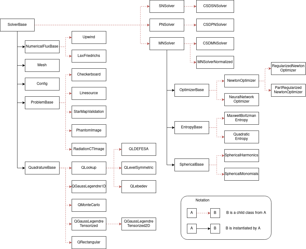
Figure 1. Class and inheritance structure of the virtual SolverBase Class. Each instantiated Solver has class members and routines specific to its numerical structure.

5.1. Solver Class

The virtual SolverBase class is the basic blueprint for all time or energy dependent finite volume solvers of the KiT-RT framework. It holds an instance of the Config, NumericalFlux, ProblemBase, QuadratureBase and Mesh class.
It controls the screen, log and volume output of the solver. The screen output provides instantaneous feedback of the solver state via the command line and gives information on the current iteration, the total mass of the system, the residual of the radiation flux as well as the flow field and whether logs and volume outputs have been written to file. The file log carries the same information as the screen output in a tabular format. Lastly, the volume output consists of vtk files with solver and problem specific solution data. The output data can be specified in the solver configuration.

Prepare outputs for Screen, Log and Volume

Solver specific pre-processing

for $i=1,\dots,n_{tf}$ do

       for $l=1,\dots,k_{rk}$ do

             Runge-Kutta pseudo iteration pre-processing

             Update numerical fluxes

             Perform finite volume step

             Update Runge-Kutta intermediate solution

            

       end for

      Iteration post-processing

       Compute Runge-Kutta solution

       Write Screen, Log and Volume output as configured

      

end for

Post-processing of output

Algorithm 1 Execution of the solver

The method Solve() of the SolverBase class drives the execution of all derived solvers by iterating over the time discretization of the numerical methods described in Section 4. This main time-iteration is displayed in Algorithm 1. Each command is specified in the derived solver classes such as the $P_{N}$ solver and does not induce any additional communication overhead for the parallelization architecture. The class PNSolver inherits from SolverBase and does not own additional instances of other custom building blocks and overwrites the sub-routines of Algorithm 1 for the $P_{N}$ equation specific numerical method, which allows for runtime solver assembly. It’s child class is the CSDPNSolver, which is the implementation of the $P_{N}$ based continuous slowing down solver, that overwrites the solver-preprocessing routines for the continuous slowing down specific energy transformation. The $P_{N}$ based solvers produce radiation flux and moments as output.

The class SNSolver adapts the sub-routines of Algorithm 1 for the ordinate based numerical methods and is the parent class of the CSDSNSolver. $S_{N}$ based solvers produce the radiation flux as output.

Lastly, the MNSolver class contains the implementation of the $M_{N}$ numerical method and holds the module SphericalBase, which controls the choice of basis functions $m(v)$ of the velocity space, the module EntropyBase, that controls the choice of entropy functional for the entropy closure and lastly the module OptimizerBase, which controls the choice of numerical optimizer used to compute the entropy closure. The class CSDMNSolver inherits from the MNSolver class and analogously overwrites the sub-routines of Algorithm 1 for the continuous-slowing down equations. $M_{N}$ based solvers produce the radiation flux, moments and dual variable of the entropy closure as output.

5.2. Mesh Class

The mesh class handles the computational meshes of the spatial discretization of the underlying differential equation. It can handle $1D$ meshes and $2D$ unstructured triangular and quadrilateral meshes in the SU2 (Palacios et al., [n. d.]) mesh format. The mesh class keeps a record of all geometry and adjacency information required for the finite volume methods with first and second order fluxes.

5.3. Computational problem class

The problem class handles the setup of computational problems and test cases. It sets the initial conditions for the solution of the numerical solver and manages space, time or energy dependent material properties for the solver. The abstract class problem base holds pointers to the Mesh and Config classes and creates instances of specific problems depending on the chosen configurations. Each implemented problem has two child classes, one for the ordinate based and one for moment based solvers. The moment based problem classes compute the moments of the initial condition and sources of the corresponding kinetic densities specified in the ordinate based problem class.
The solver framework comes with a number of pre-implemented test cases and functionalities. This includes standard 1D and 2D test cases such as line source and checkerboard for the radiative transfer solvers, as well as isotropic and directed sources with different background media which can be loaded from a user-supplied image file, for the continuous slowing down solvers. Custom test cases can be easily added by the user, based on the provided examples and our modular approach.

5.4. Quadrature Class

The virtual quadrature base class creates instances of specific numerical quadratures using its static factory method. The quadratures are intended to integrate over the velocity space of the Boltzmann equation, however, they can be applied to other use-cases as well. The implemented quadratures are distinguished by the dimension of the integrated velocity space and the integration area. Each quadrature has a specifiable order and manages the integration points in Cartesian and spherical coordinates as well as the corresponding quadrature weights. By default, the quadrature rules integrate over the unit sphere, but the integration region can be scaled.

5.5. IO/Use of Config Files

The KiT-RT solver is a command line interface based program and takes one argument, the configuration file. This file is parsed and the specified modules of the KiT-RT framework are arranged for a solver instance or another custom tool. The configuration file is a document containing option specifications of the form CONFIG_OPTION=VALUE. A solver configuration contains information about file input and output, where the location of the mesh file, the volume output files and the log files are specified. Then, the computational problem and the problem specific parameters, e.g. scattering coefficient, final time, spatial dimension and boundary conditions, are set. Next, the solver specific options are set. In the example of an $M_{N}$ solver, the choice of velocity basis, the maximal degree of the basis functions, the CFL number, spatial integration order, entropy functional, optimizer, quadrature and quadrature order are set. Finally, quantities for screen, volume and log output are specified along with their output-frequency. Example configuration files for the numerical results of Section 7 can be found in the Github Repository https://github.com/CSMMLab/KiT-RT.

5.6. Practices of modern software development

The entire solver and associated documentation is put under the version control system git (Chacon and Straub, 2014) to greatly enhance collaborative workflows. Additionally, the web-hosting service GitHub is used to provide global access to the code which is licensed under the open-source MIT license.
To further improve collaborations, the service also acts as a central host for progress and issue tracking, deployment and maintaining code integrity. The latter is obtained through automated testing in terms of unit test, which ensure the validity of smaller code instances such as functions or classes by testing predefined inputs against their expected result, or regression tests which validate the correctness of the solver as a whole based on small test problems and compare obtained results to reference solutions. These test are automatically executed every time code changes are submitted to the main development branches or if a merge request is opened.
If any of the automated tests fail for a new submit it is rejected for merging, ensuring code integrity and quality on the important development streams at all times. Combining the test information, we can further define metrics such as a test coverage describing the percentage of code lines validated by any form of testing and ultimately helps building trust in the code framework. For the KiT-RT framework the test coverage is reported to the coveralls.io service at https://coveralls.io/github/CSMMLab/KiT-RT. The KiT-RT framework features relatively modest software dependencies, but nevertheless being able to build and run the code correctly can be troublesome on many systems. To circumvent this issue, we provide a pre-configured build environment through the containerization engine Docker (Merkel, 2014). These so-called Docker containers have been developed for consistent software development and deployment and work as isolated instances with a minimal software stack comparable to lightweight virtual machines. The respective specialized docker image is also publicly available at https://hub.docker.com/r/kitrt/test.
As also mentioned previously, GitHub can also be used for the deployment of precompiled software packages and the associated documentation. The documentation is automatically is automatically generated as part of a complete software build. It is written in the reStructuredText Markup language and uses the documentation framework Sphinx (Brandl, 2021), which compiles the Markup files to a series of linked HTML files or in other words a local website. To make the website itself publicly available it is hosted by ReadTheDocs service under the URL https://kit-rt.readthedocs.io.
With all these tools in mind, the development workflow can be described as follows:
Starting on GitHub, each developer can create a new branch based on the development branch or fork the entire KiT-RT framework to obtain a personal workspace. After the developers have added their changes, they can file a merge request that will automatically be tested by the continuous integration processes and a core developer will perform a code review of all changes. Provided all test succeed and the core developer is satisfied with the added/changed code quality, it will be merged into the development branch. If enough new features have been added into the development branch, it will be merged to the master branch and the software will obtain a new version number (major or minor).

6. Parallel Scaling

In the following we investigate the parallel performance of the three base solver implementations $S_{N}$, $P_{N}$ and $M_{N}$, where we follow (Moreland and Oldfield, 2015) for the brief review of parallel scalings. The speedup of a parallel algorithm is defined as

(50) $$S(n,p)=\frac{T^{*}(n)}{T(n,p)},$$

where $T^{*}(n)$ is the execution time of the best inherently serial algorithm with input size $n$ and $T(n,p)$ the time for the parallel implementation with $p$ processing workers and input size $n$. In general the best serial algorithm may be different than the parallel algorithm, however in our application case, the finite-volume discretization scheme does not change for serial implementation.
In theory the best possible speedup is linear (Faber et al., 1986), i.e., $S(n,p)=p$, thus the measure of parallel efficiency is

(51) $$E(n,p)=\frac{S(n,p)}{p}.$$

In practise the speedup and parallel efficiency of an algorithm is limited by spawning and communication overhead of the parallel workers as well as the fraction of inherently serial code $f$, that exists in any algorithm. Thus the upper bound for the speedup is given by Amdahl (Gustafson, 2011)

(52) $$S(n,p)\leq\frac{1}{f+(1-f)/p}$$

For larger input sizes, the fraction of inherently serial code $f$ typically decreases, which enables the use of highly parallel implementations. Two common approaches to measure the parallel performance are given by the strong and weak scaling approach, where the former describes an experiment, where for fixed input size $n$ the amount of parallel workers $p$ is increased and the their timing is measured, which directly results in the speedup of Eq. (50). The latter increases the input size $n$ proportionally to the worker count $p$. A perfectly parallel algorithm would have a constant parallel time $T(n,p)$.

The philosophy of the parallel implementation of the solvers of this work are based on the independence of the performed computations of the grid cells. As Algorithm 1 displays, during one (pseudo) time iteration of a solver, a set of instructions are calculated. Each instruction can be carried out independently for each grid cell and only in between two instruction sets, communication between parallel workers need to be established. Therefor, the parallel implementation spawns a set of parallel workers with shared memory access and distributes the spatial grid among them to carry out the current instruction. The input size $n$ is thus given by the number of grid cells of the spatial discretization.

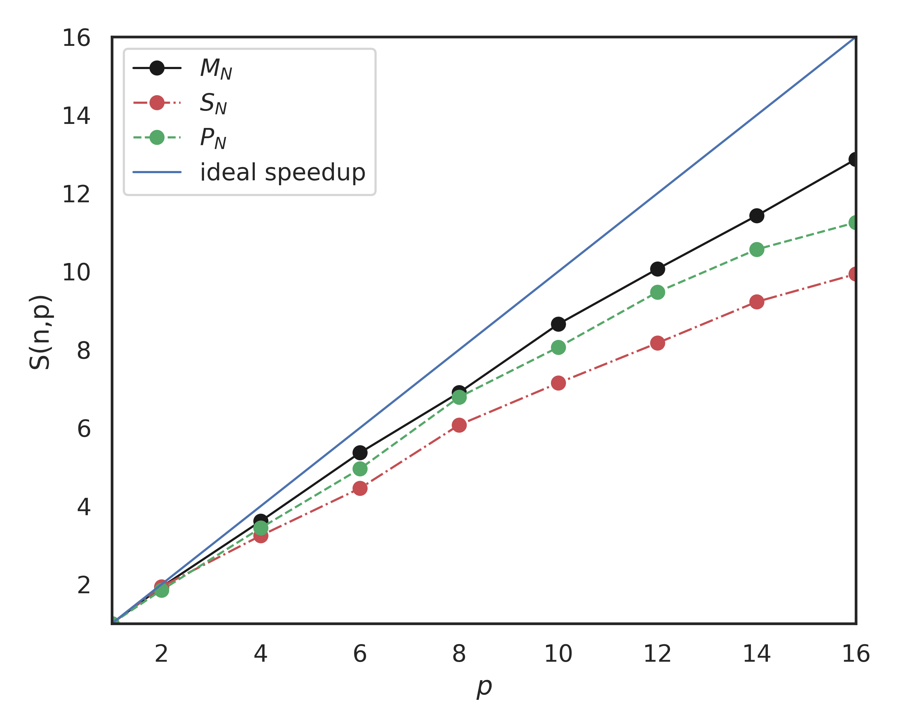
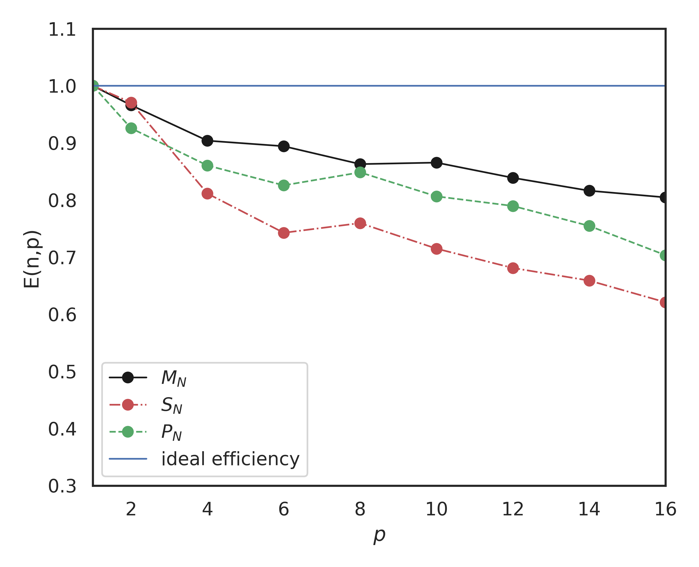
Figure 2. Strong parallel scaling (left) and parallel efficiency (right) for the $M_{N}$, $S_{N}$ and $P_{N}$ solver

We perform a strong parallel scaling study for the implementation of the $M_{N}$, $S_{N}$ and $P_{N}$ solver on the Linesource test case, as described in Section 7.1, with a fixed unstructured triangular mesh of size $n=578290$ and varying number of shared memory parallel workers $p$. We choose $p=1,\dots,16$, furthermore, the solvers allocated memory does not exceed the systems memory. Figure. 2 shows a comparison of the solvers parallel scalings and efficiency. It is apparent, that the $M_{N}$ solver enjoys the highest speedup even for a high parallel worker count, while the $P_{N}$ and $S_{N}$ solver experience diminishing returns for more than $p=12$ workers. The performance of the continuous slowing down solver implementations follows the corresponding base solver performance, since the same spatial, velocity and (pseudo) temporal discretizations are used.

7. Validation

For validation and a comparison of the implemented solvers, we consider a selection of the test cases provided within the problem class (5.3). The $S_{N}$ solver is validated with a comparison with Kinetic.jl (Xiao, 2021b, a). The continuous slowing down solvers are further compared to a reference Monte Carlo solution computed using TOPAS (Perl et al., 2012) as well as the validated spherical harmonics solver StaRMAP (Seibold and Frank, 2014).

7.1. Inhomogeneous linesource

In the following, we compare the numerical results of our framework to a Monte Carlo solution computed using TOPAS (Perl et al., 2012) as well as the staggered-grid spherical harmonics solver StaRMAP (Seibold and Frank, 2014). The problem considered is an inhomogeneous linesource testcase, which extends the classical linesource benchmark (Ganapol, 1999, 2008) to a steady-state but energy dependent setting. As background density, a piece-wise constant function $\rho(\mathbf{x})=1+4\cdot\mathbbm{1}_{X_{u}}(\mathbf{x})$ for $\mathbf{x}\in[0,1]^{2}$ is chosen. Here $\mathbbm{1}_{A}:X\rightarrow\mathbb{R}$ denotes the indicator function for the set $A$. The upper part of the spatial domain on which we prescribe a reduced density is defined as $X_{u}=[0,1]\times[0.56,1]$. At a maximal energy of $E_{\mathrm{max}}=1$, a particle beam is positioned in the center of the spatial domain $\mathbf{x}_{0}=\frac{1}{2}(1,1)^{T}$, which is modelled as

$$\psi(E_{\mathrm{max}},\mathbf{x},\mathbf{\Omega})= \frac{1}{2\pi\sigma^{2}}\exp\left(-\frac{\|\mathbf{x}-\mathbf{x}_{0}\|^{2}}{2\sigma^{2}}\right)$$

$$\psi(E_{\mathrm{max}},\mathbf{x},\mathbf{\Omega})= 0\quad\text{ for }\mathbf{x}\in\partial X.$$

Here a standard deviation of $\sigma=0.01$ is chosen to obtain a sharp particle beam in the center. The spatial grid for all deterministic methods is a structured rectangular grid with $300^{2}$ cells. Due to the functionality of the Monte-Carlo software, we use a three-dimensional grid and project the $x_{3}$-domain onto the $x_{1}-x_{2}$ plane. To allow for feasible costs, the Monte-Carlo method uses a coarser grid resolution of 100 spatial cells per dimension and 100000 Monte-Carlo runs are computed to reduce statistical noise. The $S_{N}$ solver uses a product quadrature rule of order $20$ for the streaming step and spherical moments up to order $8$ to compute scattering terms. Similarly, the $P_{N}$ solver employs spherical moments up to order $8$. The time step restriction of all deterministic methods picks a CFL number of $0.7$. All methods are second order in space and first order in time.

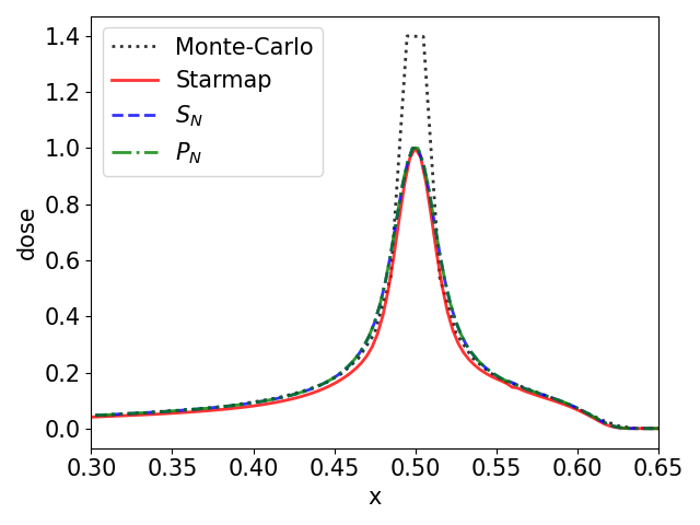
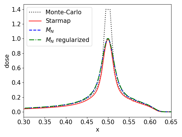
Figure 3. Comparison of simulation results of deterministic and stochastic methods.

The resulting dose profile is plotted in Figure 3 along the $x_{2}$-axis in the interval $x_{2}\in[0.3,0.65]$. It is observed that the dose drops in the transition between densities $1$ and $5$. All methods show a similar behaviour and (except for the center region) agree well with the Monte-Carlo results. Note that the increased Monte-Carlo dose results from the coarser mesh, leading to a coarser initial particle distribution. Moreover, it is observed that the regularized $M_{N}$ method seems to coincide with its non-regularized counterpart.

7.2. Checkerboard

The checkerboard test case mimics a nuclear reactor block with a strong radiative source in the domain center, which is denoted by $\mathbf{X}_{q}$, and several highly absorptive regions $\mathbf{X}_{a}$ placed in a checkerboard pattern it.

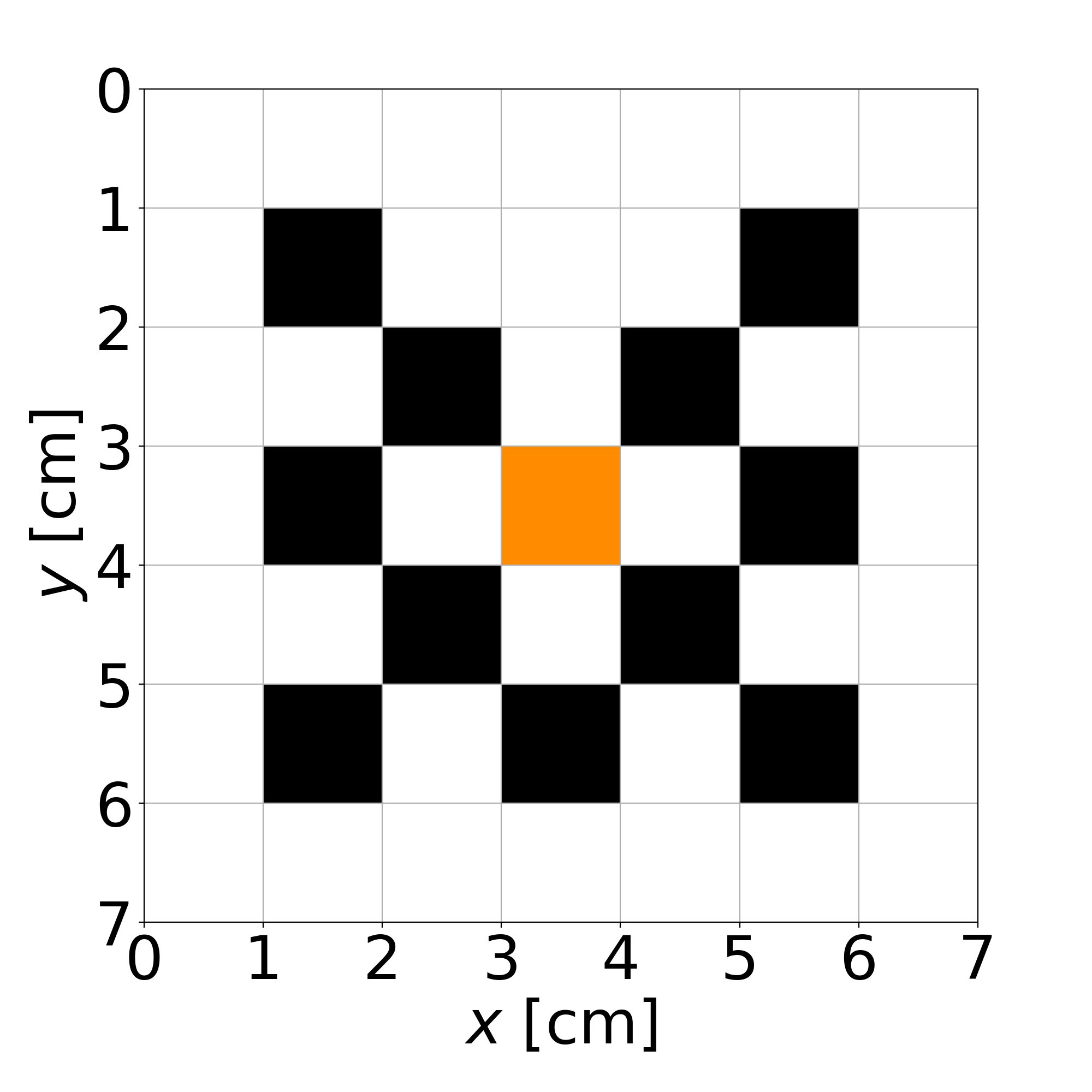
Figure 4. Layout of the two dimensional checkerboard test case.

The spatial layout of this two dimensional test case can be found in Figure 4, where the source region $\mathbf{X}_{q}$ is marked orange and the absorption regions $\mathbf{X}_{a}$ are marked black. The corresponding time dependent linear Boltzmann equation reads

(53) $$\partial_{t}\psi+\mathbf{\Omega}\nabla_{\mathbf{x}}\psi+\Sigma_{t}=\int_{\mathbb{S}^{2}}\Sigma_{s}(t,\mathbf{x},\mathbf{\Omega},\mathbf{\Omega}_{*})\psi(\mathbf{\Omega}_{*})\;\mathrm{d}\mathbf{\Omega}_{*}+q(\mathbf{t,\mathbf{x},\Omega})$$

for $\mathbf{x}\in[0,7]^{2}$, $t\in[0,10)$ and $\mathbf{\Omega}\in P_{\mathbb{R}^{2}}(\mathbb{S}^{2})$. This corresponds to Eq. (9) with $\rho(\mathbf{x})=1$. We equip the equation with Dirichlet boundary conditions and initial condition

(54) $$\psi(t,\mathbf{x},\mathbf{\Omega})= 0,\qquad\mathbf{x}\in\partial\mathbf{X}$$

(55) $$\psi(t,\mathbf{x},\mathbf{\Omega})= 0,\qquad t=0$$

to obtain a well posed problem. Furthermore, the scattering kernel $k$ and source term $q$ are assumed to be isotropic and constant in time. The scattering cross and absorption cross sections are given by

(56) $$\Sigma_{s}(\mathbf{x})=\begin{cases}0&\mathbf{x}\in X_{a}\\ 1&\text{else}\end{cases},\qquad\Sigma_{t}(\mathbf{x})=\begin{cases}10&\mathbf{x}\in\mathbf{X}_{a}\\ 1&\text{else}\end{cases},$$

and the isotropic source is given by

(57) $$q(\mathbf{x},\mathbf{\Omega},t)=\begin{cases}1&\mathbf{x}\in\mathbf{X}_{q}\\ 0&\text{else}\end{cases}.$$

We create a unstructured triangular mesh with $25000$ cells to discretize the spatial domain with regard to the absorption and source regions, such that the region boundaries coincide with the mesh faces. The simulation is computed until final time $t_{f}=10$ using various solver configurations. All employed solvers use a second order upwind flux as the spatial discretization and a second order explicit Runge Kutta scheme for temporal discretization with CFL number equals $0.45$, since $M_{N}$ solvers with non-regularized entropy closure require a CFL number smaller than $0.5$ for stability (Kusch et al., 2019; Alldredge et al., 2012; Kristopher Garrett et al., 2015). The solution computed at final time $t_{f}=10$ is displayed in Fig. 5, where we can see the scalar flux

(58) $$\Psi(\mathbf{x},t)=\int_{\mathbb{S}}^{2}\psi\;\mathrm{d}\mathbf{\Omega},$$

in the countour plot. The radiation flux is highest at the source region $\mathbf{X}_{q}$ and almost zero in the absorption region $\mathbf{X}_{a}$ for all solvers. Towards the top of the domain, the radiation travels freely, whereas towards the left, right and bottom, the radiation expansion is damped by absorption regions.

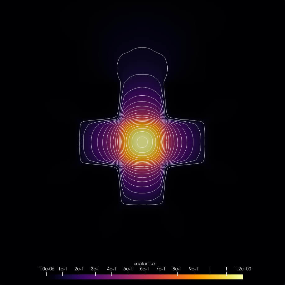
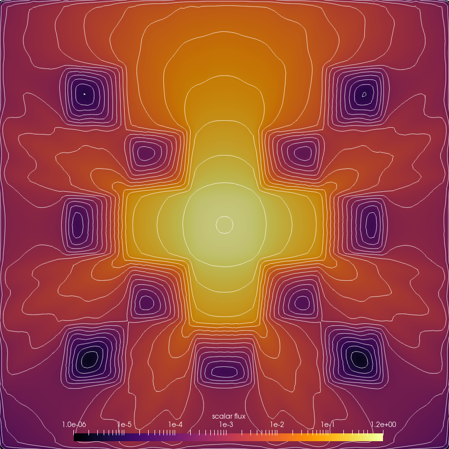
Figure 5. Simulation results for the S₁₀ solver in linear scale and log scale.

Figure 5 shows the solution computed with the S₁₀ solver with an order $10$ tensorized Gauss Legendre Quadrature. On the logarithmic scale plot, one can see ray effects right outside the chokepoints between the absorption regions, which are typical artifacts for $S_{N}$ (Camminady et al., 2019). We validate the S₁₀ solver against the implementation of the kinetic.jl framework (Xiao, 2021b), and display the vertical cross section of the KiT-RT and kinetic.jl bases solution at final time $t_{f}$ in Fig. 6 using the same triangular mesh. We can see, that the deviation between implementations is below the $1\mathrm{e}{-3}$, which is the characteristic length of a grid cell.

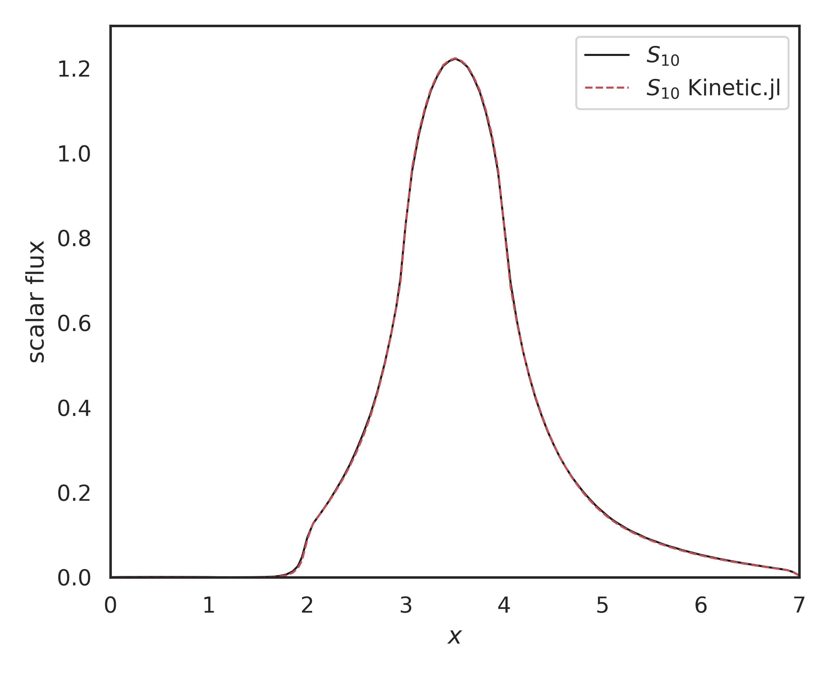
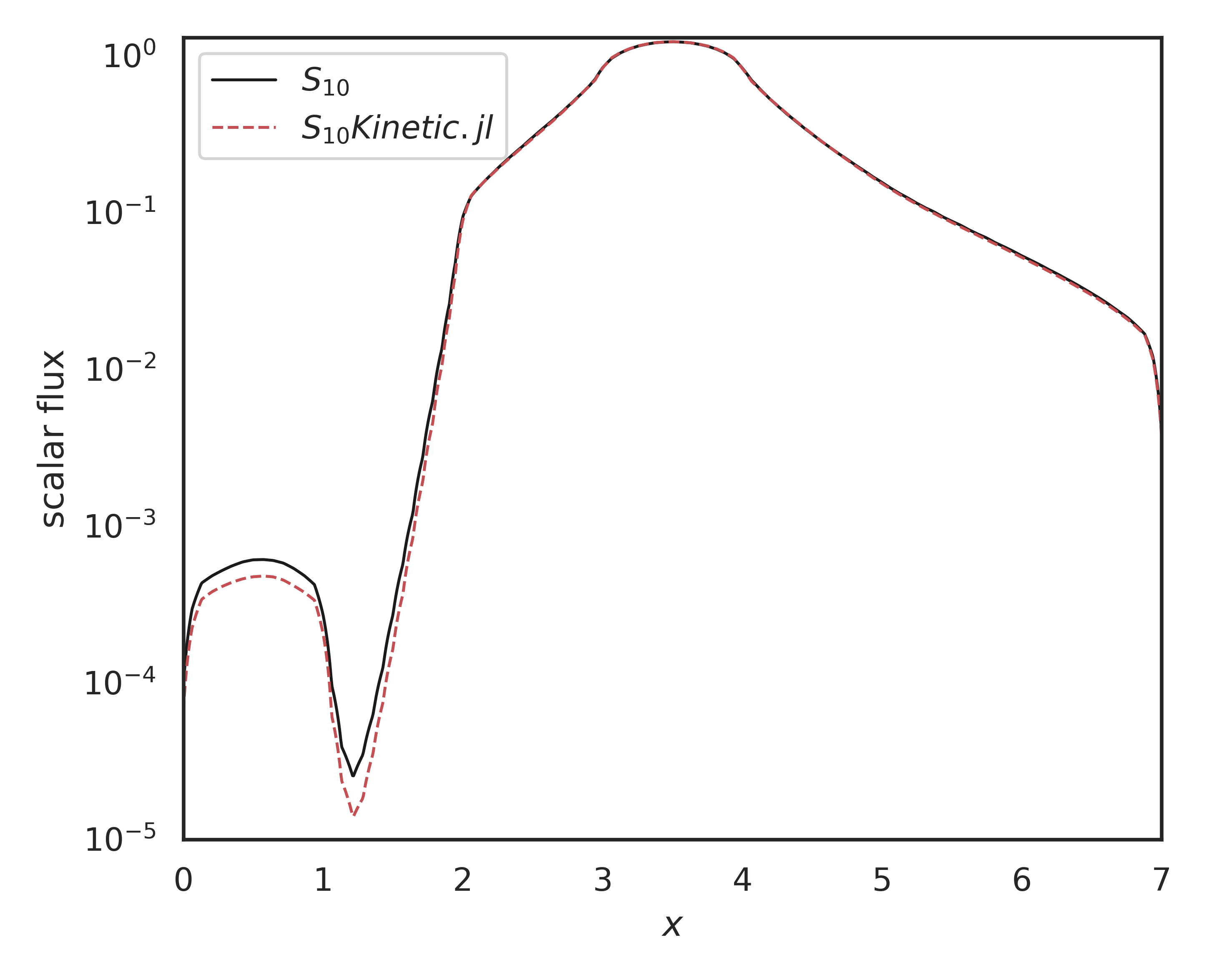
Figure 6. Vertical cross section through the solution of the S₁₀ method. Comparison of the KiT-RT and kinetic.jl packages.

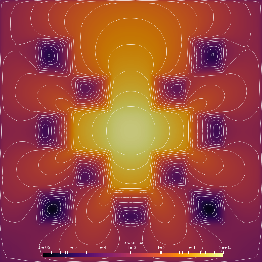
Figure 7. Simulation results for the P₅ solver in linear scale and log scale.

Figure 7 displays the solution computed with the $P_{5}$ solver using an order $5$ Spherical Harmonics basis. Compared to the $S_{10}$ solution, there are no ray effects visible at the chokepoints between absorption regions.

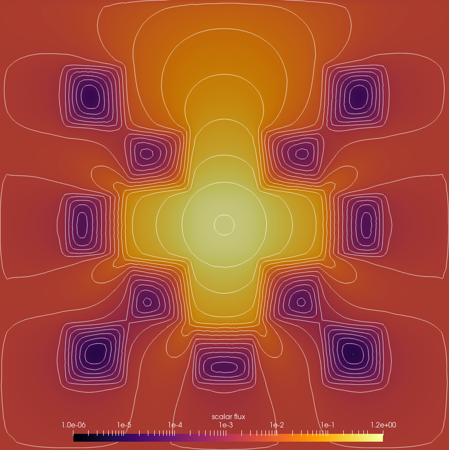
Figure 8. Simulation results for the M₃ solver with spherical harmonics basis in linear scale and log scale.

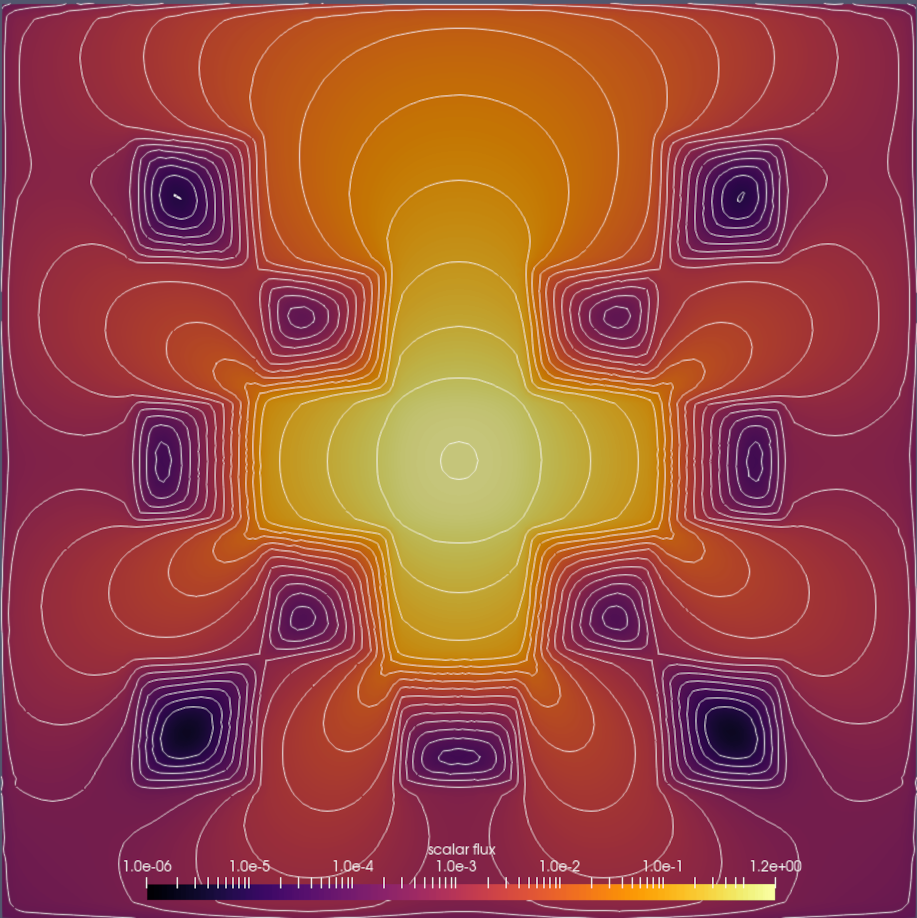
Figure 9. Simulation results for the M₃ solver with spherical harmonics basis and regularized entropy in linear scale and log scale.

We show now the solution for different entropy based moment, i.e., $M_{N}$ solvers, that use an order $10$ tensorized Gauss Legendre quadrature to evaluate the kinetic flux. Figure 8 displays a M₃ solution using an order $3$ spherical harmonics moment basis computed with a Newton optimizer with line-search configured to accuracy $1\mathrm{e}{-7}$. The same solver configuration is displayed in Figure 9, where the entropy closure is replaced by the partial regularized minimal entropy problem of Eq. (19) with the regularizer $\gamma$ set to $1e-3$ and a non-regularized moment of order zero. While on the linear scale plots, both solutions are similar, on the log scale plots, one can see that the regularized $M_{N}$ solver computes much lower values within the absorption regions. Furthermore, the log plot shows that the regularized $M_{N}$ solution oscillates slightly in regions with small scalar fluxes. Figure 10 shows a direct comparison of a vertical cross section using all four presented solvers. In the vast majority of the spatial domain, the solutions correspond well, with the exception of absorption regions, i.e., $x\in[1,2]$, where the $M_{3}$ solution computes slightly bigger values and the regularized $M_{3}$ solution captures the absorption region slightly better than the reminding solvers.

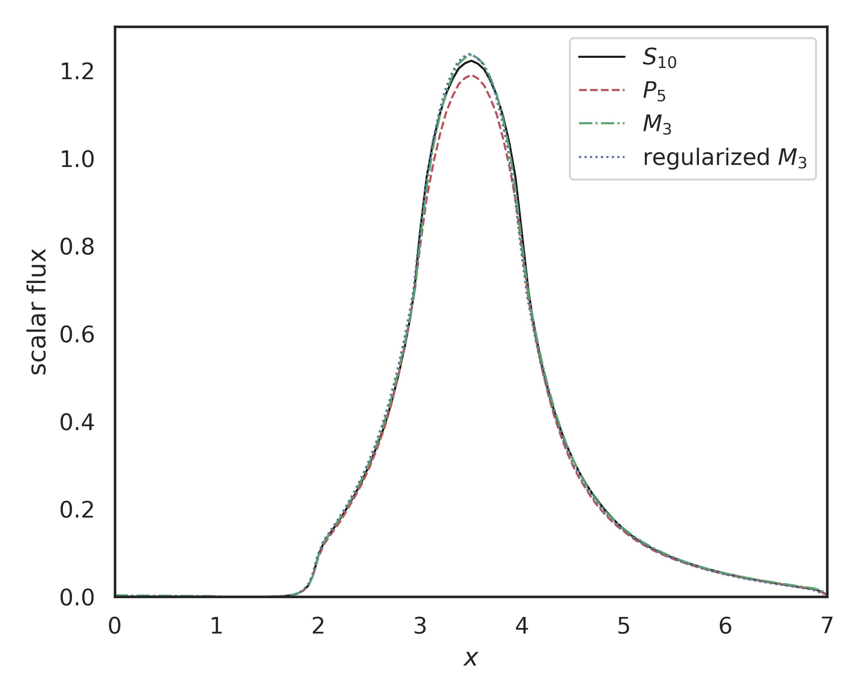
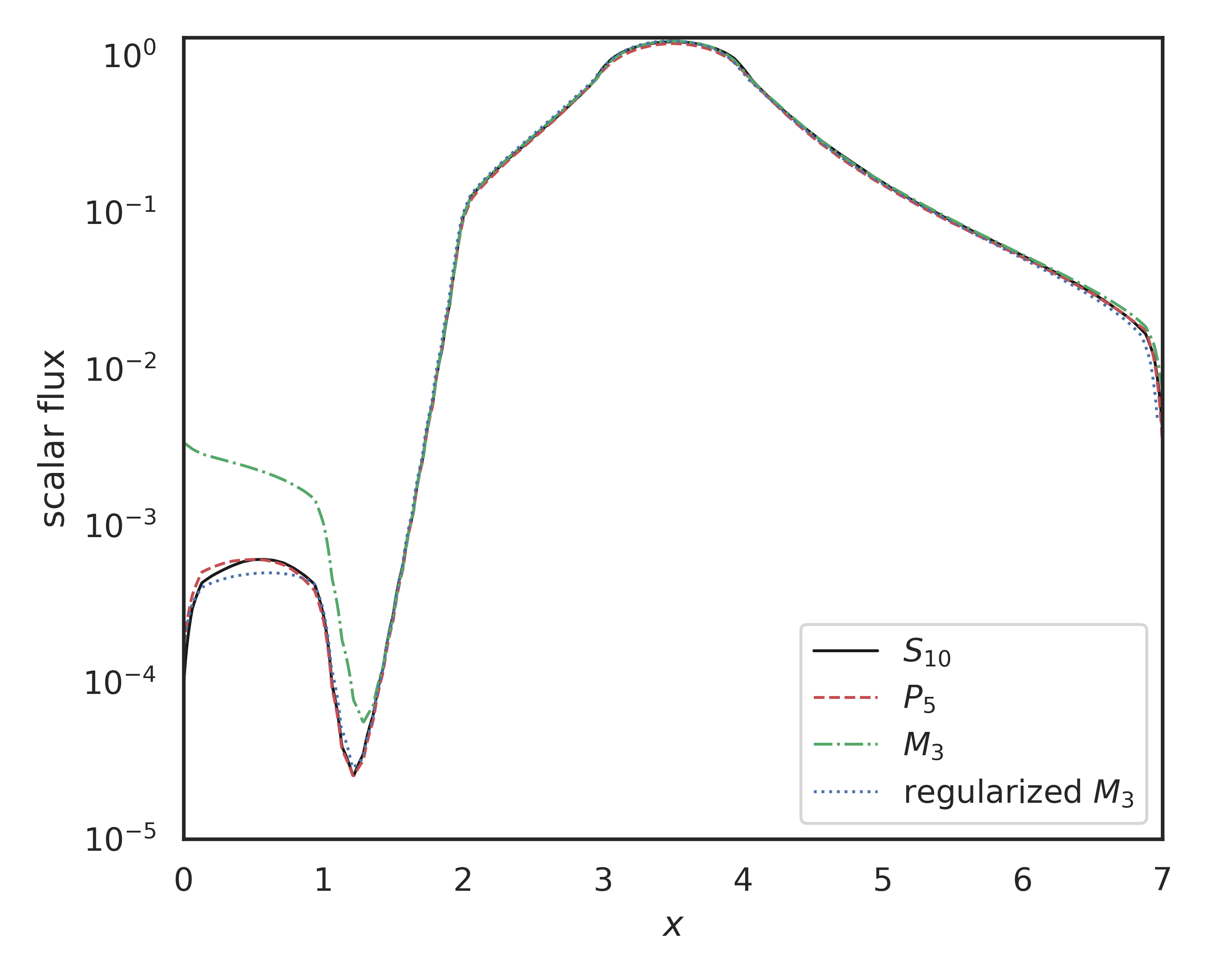
Figure 10. Vertical cross section through the solution of the checkerboard test case. Comparison of the $S_{10}$, $P_{5}$ ,$M_{3}$ and regularized $M_{3}$ solver .

Next we compare a non-regularized M₁ solver using a monomial basis of order $1$ and a Newton solver based entropy computation, shown in Fig. 11, with a similar solver configuration, which employs a neural network to compute the entropy closure, shown in Fig 12. Various data driven entropy closures have been introduced by (Schotthöfer et al., 2022; Porteous et al., 2021). In the KiT-RT package we have compiled the trained networks by (Schotthöfer et al., 2022) to C++ and have implement a fast tensorflow (Abadi et al., 2015) backend for seamless integration into the KiT-RT framework. The neural network used in the simulation of Fig 12 is an input-convex architecture. Both, the Newton based and neural network based solution correspond well. As Fig. 13 shows, only in at the top of the domain, i.e., at $x\approx 6.5$ in the cross section plot, we see a small deviation between the methods. In this region at the wave-front of the radiative transport, the moments of the kinetic equation are close to the boundary of the realizable set, where on the one hand, the Newton based solver needs more iterations and thus more wall time to compute the solution to the optimization problem, and on the other hand, the neural network accuracy declines.

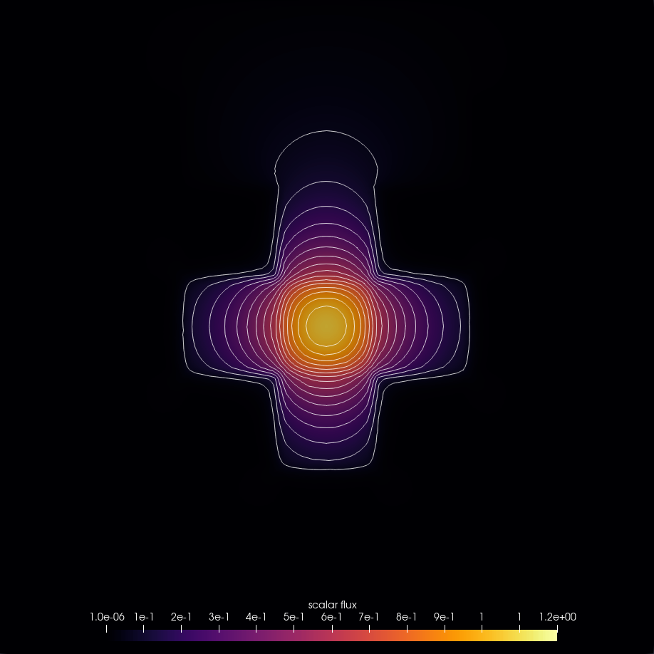
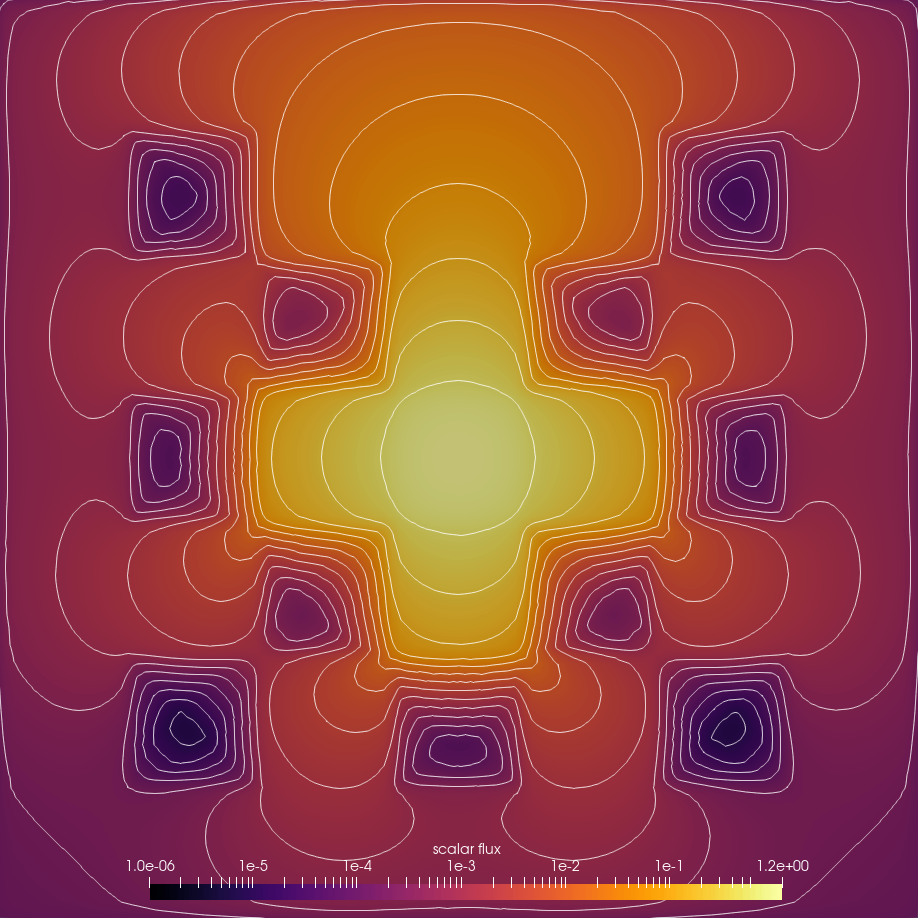
Figure 11. Simulation results for the $M_{1}$ solver with monomial basis in linear scale and log scale.

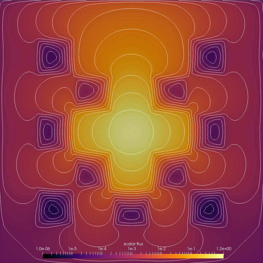
Figure 12. Simulation results for the $M_{1}$ solver with monomial basis and neural network based entropy computation in linear scale and log scale.

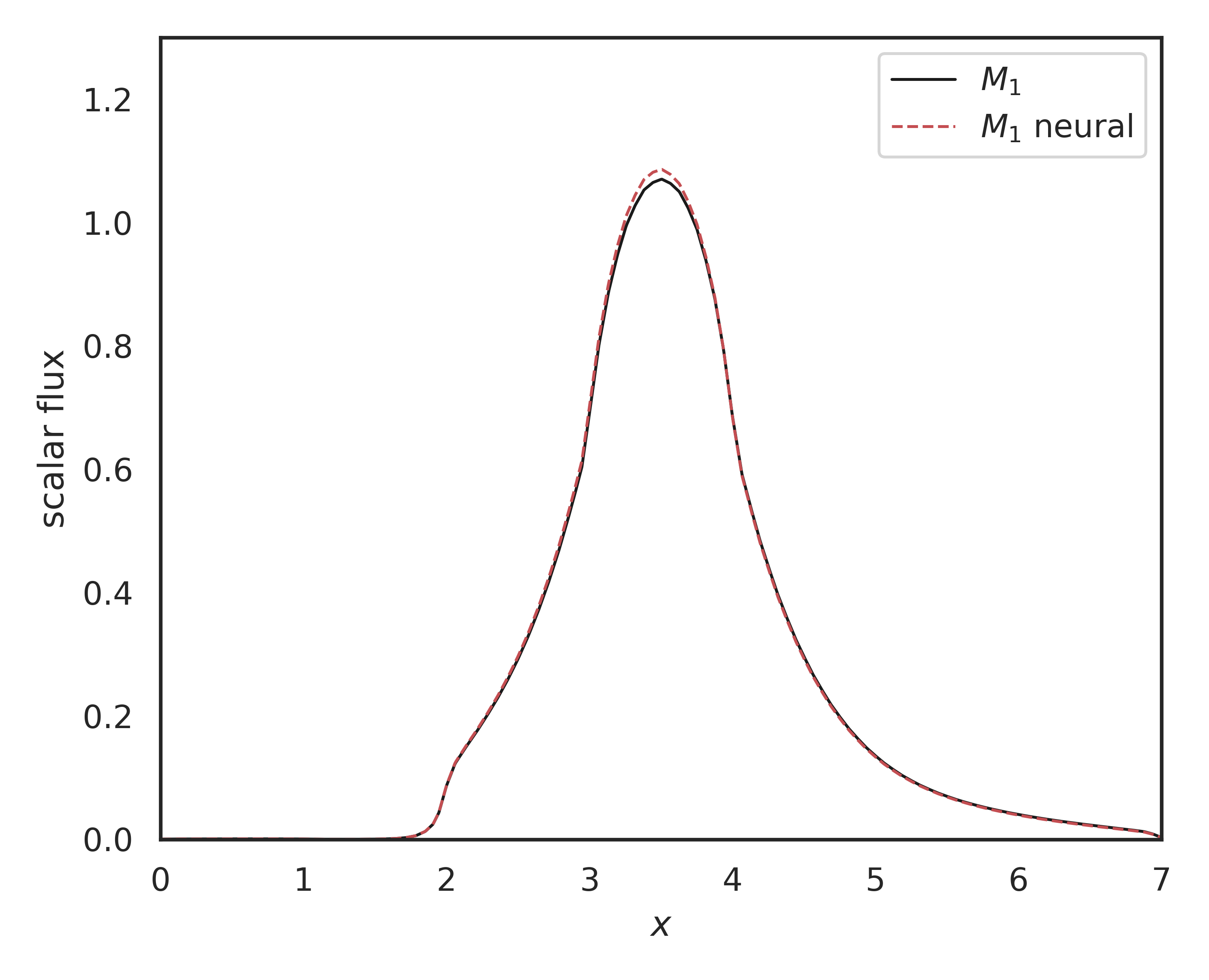
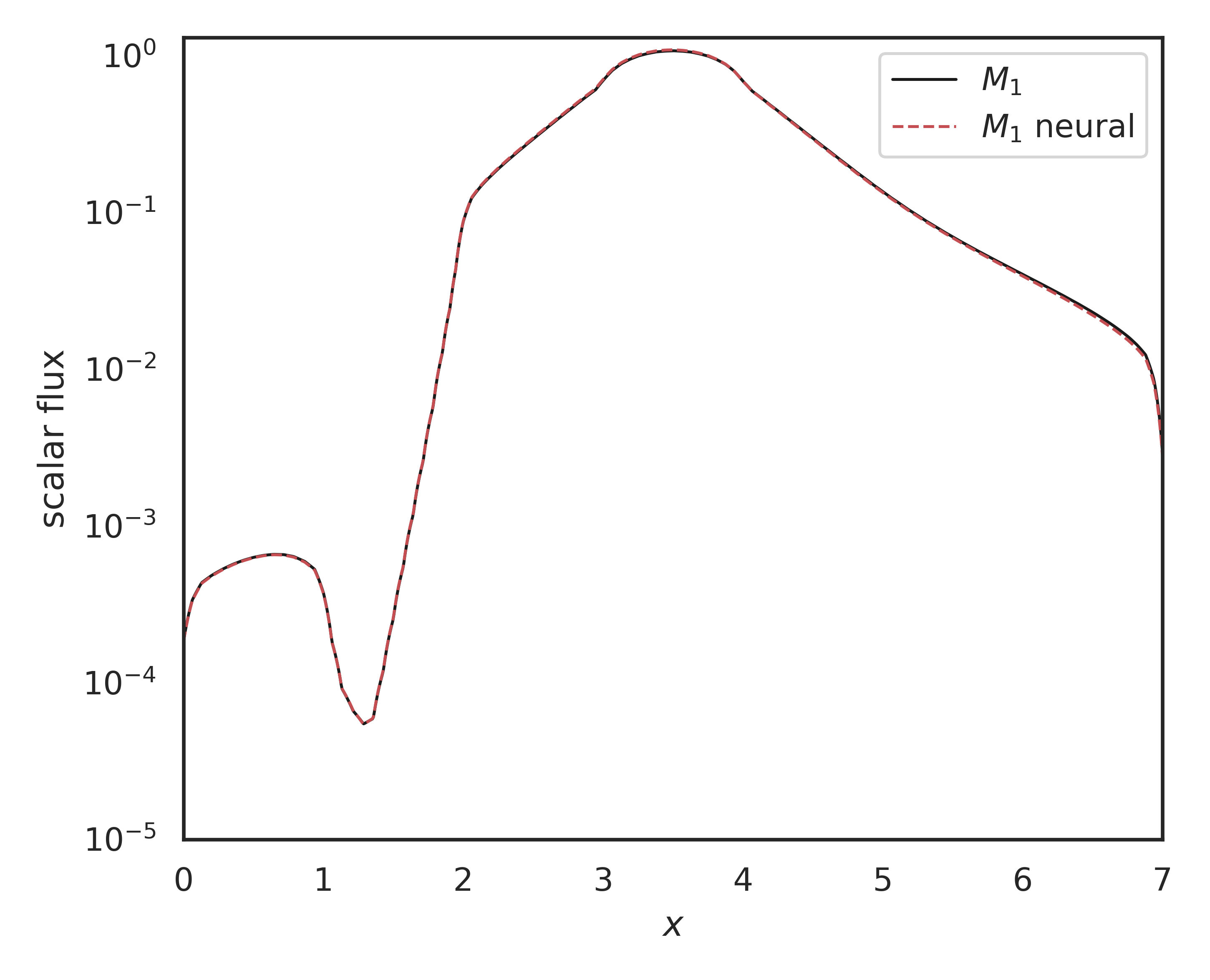
Figure 13. Cross section comparison of the Checkerboard test case using the $M_{1}$ and neural network based $M_{1}$ method.

Neural network based entropy closures are constructed to accelerate the time consuming $M_{N}$ method. In the following we validate the speedup through the neural network entropy closure using a larger mesh of $700000$ grid cells, since in  (Schotthöfer et al., 2022) it is shown, that the due to data transformation to tensorflow tensors, the speedup is faster for higher data-set sizes. The time consumption of the $M_{1}$ and neural network based $M_{1}$ solver is illustrated in Table 1, where one can see that the neural network based closure accelerates the compuational time by $89.33$-$87.01$%.

Table 1. Timings of the neural network based $M_{1}$ solver compared to the Newton based $M_{1}$ solver

	$M_{1}$ Newton	$M_{1}$ neural network	runtime reduction
$4$ cores	$757.88979$	$80.810305$	$89.33$%
$12$ cores	$258.6485$	$33.606152$	$87.01$%

7.3. Beam in 2D patient CT

Having validated the CSD solvers against StarMAP and a Monte Carlo framework in section 7.1, we now examine a realistic 2D CT scan of a lung patient as a proof of concept for the application of our framework to radiation therapy computations. The patient data was retrieved from an open source data set (Li et al., 2020) in The Cancer Imaging Archive (TCIA) (Clark et al., 2013). The patient is irradiated with an electron beam of $E_{\text{max}}=20$ MeV. We model this beam as the initial condition

$$\psi(E_{max},\mathbf{x},\mathbf{\Omega})=\frac{1}{(2\pi)^{3/2}\sigma_{\Omega_{2}}\sigma_{x}\sigma_{y}}\cdot\exp(-(\mu_{\Omega_{2}}-\Omega_{2})^{2}/2\sigma_{\Omega_{2}})\cdot\exp(-(\mu_{x_{1}}-x_{1})^{2}/2\sigma_{x_{1}})\cdot\exp(-(\mu_{x_{2}}-x_{2})^{2}/2\sigma_{x_{2}}),$$

where $(\mu_{x_{1}},\mu_{x_{2}})=(2.5\text{cm},5.8\text{cm})$ is the beam position within the $6\text{cm}x6\text{cm}$ domain and $\mu_{\Omega_{2}}=\frac{\pi}{2}\text{rad}$ is the beam direction. The remaining parameters are chosen as $\sigma_{x_{1}}=\sigma_{x_{2}}=\sigma_{\Omega_{2}}=0.1$. To determine a tissue density $\rho$ for given gray-scale values of the CT image, we set the maximum density, represented by white pixels, to the density of bone $\rho_{\text{bone}}=1.85\text{ g}/\text{cm}^{3}$. The remaining tissue is scaled such that the minimum pixel value of zero corresponds to a minimal density of $\rho_{\text{min}}=0.05\text{ g}/\text{cm}^{3}$. This corresponds approximately to the lower bound of observed lung densities (Kohda and Shigematsu, 1989).

Figure 14 compares the normalized dose for a CSD $S_{13}$, $P_{13}$ and $M_{5}$ solver. While all methods show similar behaviour and are able to capture the effects of heterogeneities in the patient density, some differences e.g. in the maximum depth of the $S_{13}$ solution compared to $P_{13}$ and $M_{5}$ or the shape of the lowest two isolines can be observed. The cross sections in figure 15 further show that the $S_{13}$ dose has a lower maximum and higher minimum value than the $M_{5}$ and to a lesser extent also $P_{13}$ solutions.

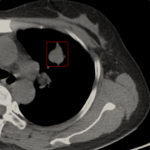
(a) CT scan

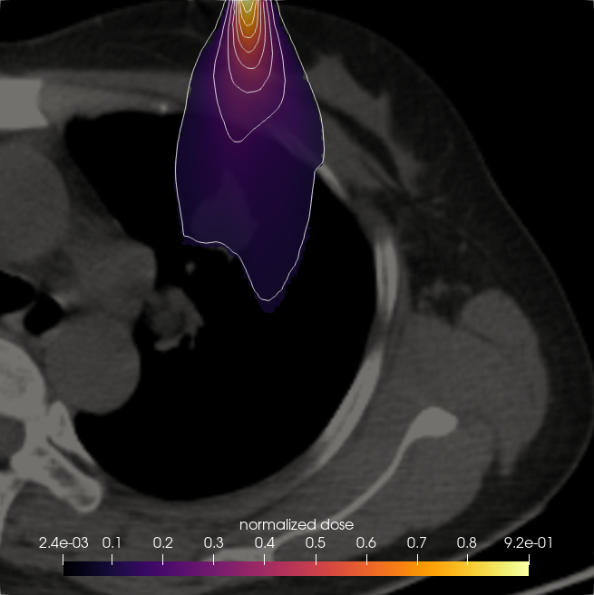
(b) $S_{13}$

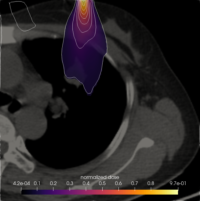
(c) $P_{13}$

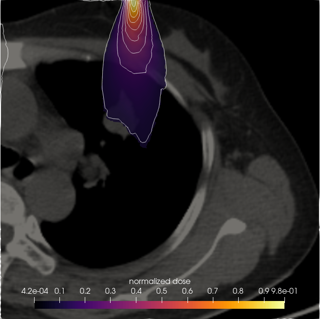
(d) $M_{5}$

Figure 14. Patient CT scan with lung tumor (red box) (a) as well as corresponding simulation results for the $S_{13}$, $P_{13}$ and $M_{5}$ solver with spherical harmonics basis and partially regularized entropy.

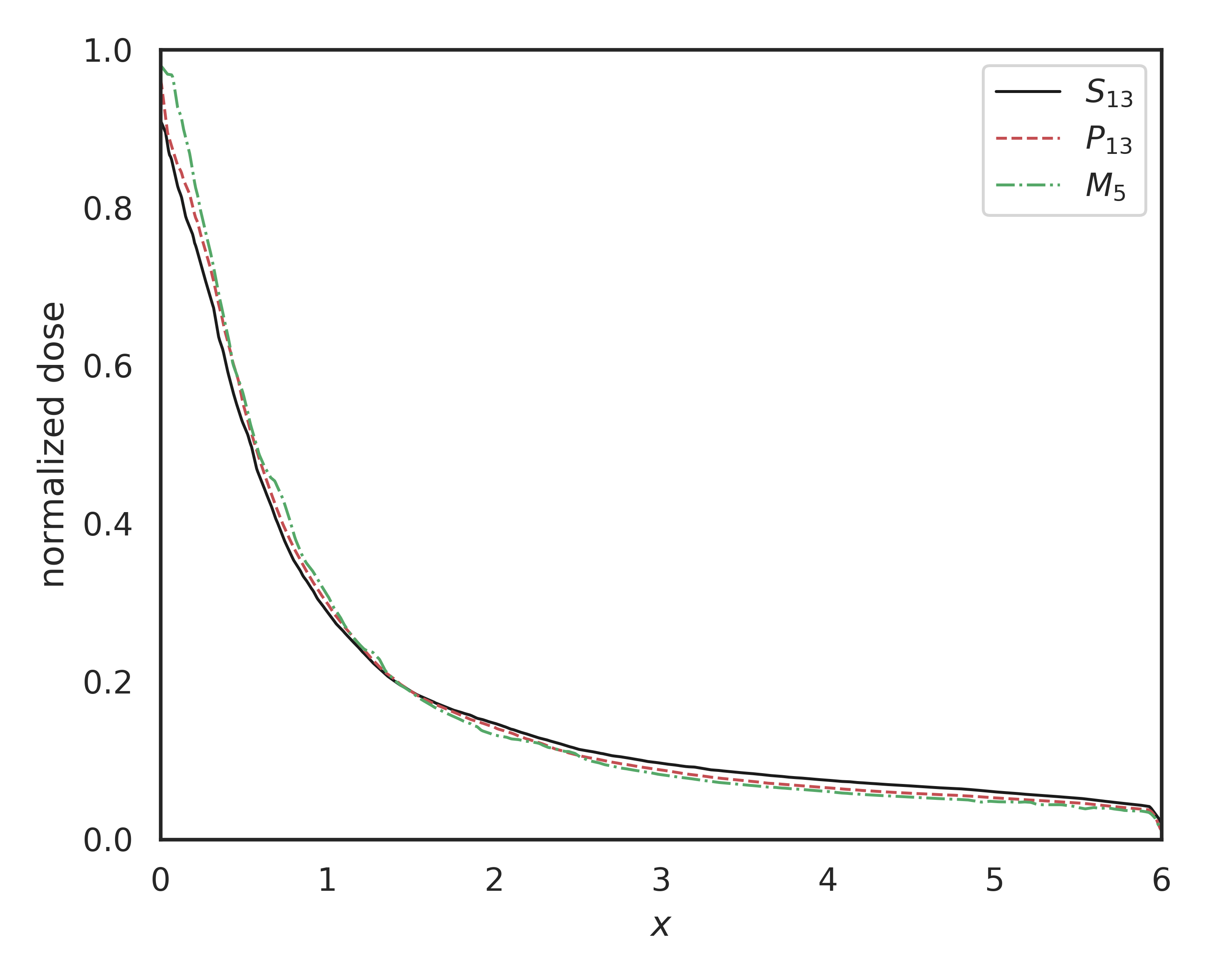
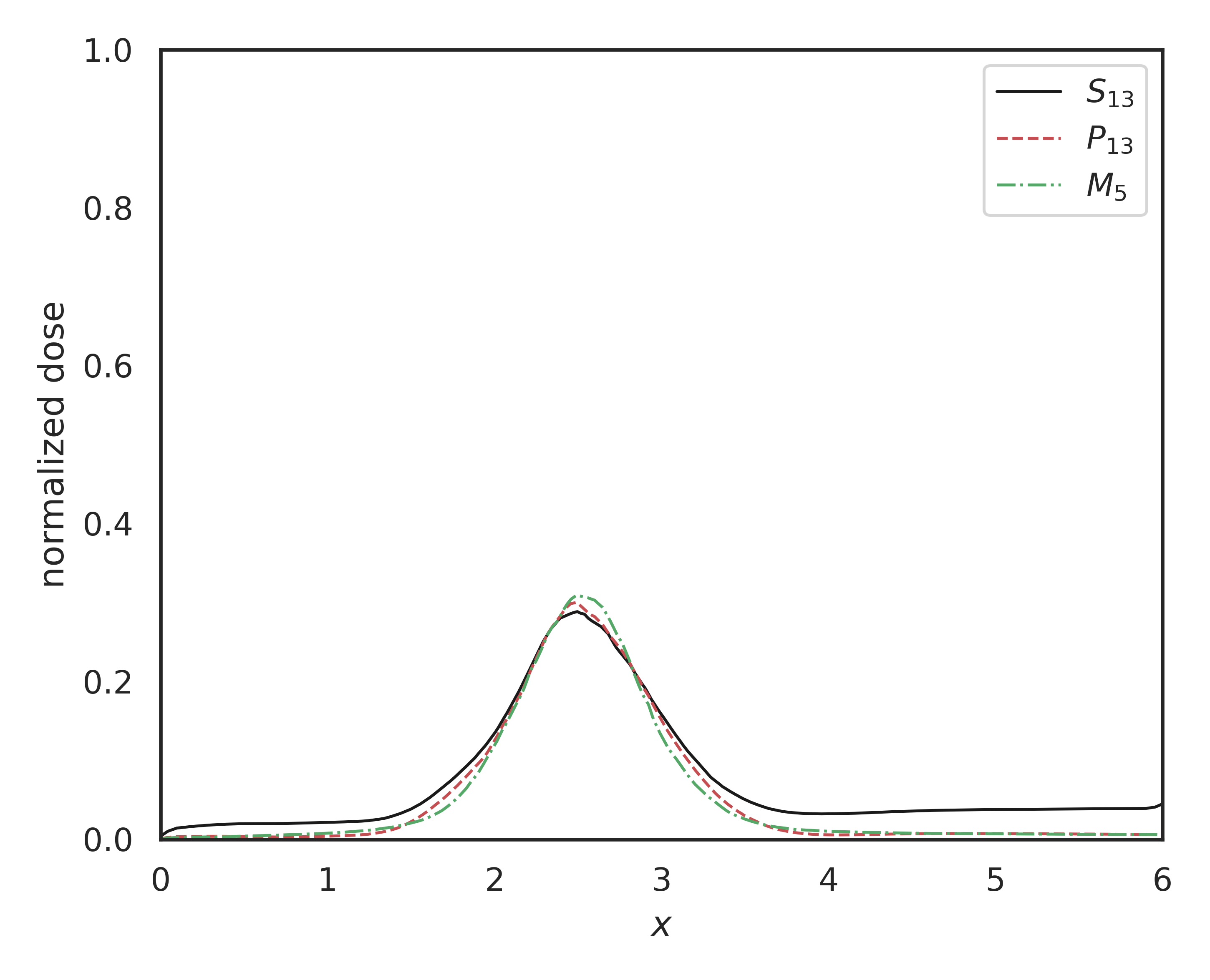
Figure 15. Vertical (at $x=2.5$cm) and horizontal (at $y=5$cm) cross section through the normalized dose in the patient CT. Comparison of the $S_{13}$, $P_{13}$ and partially regularized $M_{5}$ solver.

8. Conclusion

In this work, we have presented a collection of deterministic transport solvers for radiation therapy applications. The methods agree well with results obtained with conventional radiation therapy codes. Due to the use of polymorphism, we are able to guarantee a straight forward extension to further numerical methods, which facilitates the investigation of novel radiation therapy solvers and their comparison to conventional methods.

References

- (1)
- Abadi et al. (2015) Martín Abadi, Ashish Agarwal, Paul Barham, Eugene Brevdo, Zhifeng Chen, Craig Citro, Greg S. Corrado, Andy Davis, Jeffrey Dean, Matthieu Devin, Sanjay Ghemawat, Ian Goodfellow, Andrew Harp, Geoffrey Irving, Michael Isard, Yangqing Jia, Rafal Jozefowicz, Lukasz Kaiser, Manjunath Kudlur, Josh Levenberg, Dandelion Mané, Rajat Monga, Sherry Moore, Derek Murray, Chris Olah, Mike Schuster, Jonathon Shlens, Benoit Steiner, Ilya Sutskever, Kunal Talwar, Paul Tucker, Vincent Vanhoucke, Vijay Vasudevan, Fernanda Viégas, Oriol Vinyals, Pete Warden, Martin Wattenberg, Martin Wicke, Yuan Yu, and Xiaoqiang Zheng. 2015. TensorFlow: Large-Scale Machine Learning on Heterogeneous Systems. https://www.tensorflow.org/ Software available from tensorflow.org.
- Abu-Shumays (2001) IK Abu-Shumays. 2001. Angular quadratures for improved transport computations. Transport Theory and Statistical Physics 30, 2-3 (2001), 169–204.
- Aftosmis et al. (1995) Michael Aftosmis, Datta Gaitonde, and T. Sean Tavares. 1995. Behavior of linear reconstruction techniques on unstructured meshes. AIAA Journal 33, 11 (1995), 2038–2049. https://doi.org/10.2514/3.12945 arXiv:https://doi.org/10.2514/3.12945
- Alldredge et al. (2018) Graham W. Alldredge, Martin Frank, and Cory D. Hauck. 2018. A regularized entropy-based moment method for kinetic equations. arXiv:1804.05447 [math.NA]
- Alldredge et al. (2012) Graham W. Alldredge, Cory D. Hauck, and André L. Tits. 2012. High-Order Entropy-Based Closures for Linear Transport in Slab Geometry II: A Computational Study of the Optimization Problem. SIAM Journal on Scientific Computing 34, 4 (2012), B361–B391. https://doi.org/10.1137/11084772X arXiv:https://doi.org/10.1137/11084772X
- Amos et al. (2016) Brandon Amos, Lei Xu, and J. Zico Kolter. 2016. Input Convex Neural Networks. CoRR abs/1609.07152 (2016). arXiv:1609.07152 http://arxiv.org/abs/1609.07152
- Andreo (1991) P Andreo. 1991. Monte Carlo techniques in medical radiation physics. 36, 7 (jul 1991), 861–920. https://doi.org/10.1088/0031-9155/36/7/001
- Barnard et al. (2012) Richard Barnard, Martin Frank, and Michael Herty. 2012. Optimal radiotherapy treatment planning using minimum entropy models. Appl. Math. Comput. 219, 5 (2012), 2668–2679.
- BARTH and JESPERSEN ([n. d.]) TIMOTHY BARTH and DENNIS JESPERSEN. [n. d.]. The design and application of upwind schemes on unstructured meshes. https://doi.org/10.2514/6.1989-366 arXiv:https://arc.aiaa.org/doi/pdf/10.2514/6.1989-366
- Börgers (1998) Christoph Börgers. 1998. Complexity of Monte Carlo and deterministic dose-calculation methods. Physics in Medicine & Biology 43, 3 (1998), 517.
- Brandl (2021) Georg Brandl. 2021. Sphinx documentation. URL http://sphinx-doc.org/ (2021).
- Camminady et al. (2019) Thomas Camminady, Martin Frank, Kerstin Küpper, and Jonas Kusch. 2019. Ray effect mitigation for the discrete ordinates method through quadrature rotation. J. Comput. Phys. 382 (2019), 105–123.
- Camminady et al. (2021) Thomas Camminady, Martin Frank, and Jonas Kusch. 2021. Highly uniform quadrature sets for the discrete ordinates method. Nuclear Science and Engineering (2021).
- Case and Zweifel (1967) Kenneth M Case and Paul Frederick Zweifel. 1967. Linear transport theory. (1967).
- Chacon and Straub (2014) Scott Chacon and Ben Straub. 2014. Pro git. Springer Nature.
- Clark et al. (2013) K Clark, B Vendt, K Smith, J Freymann, J Kirby, P Koppel, S Moore, S Phillips, D Maffitt, M Pringle, L Tarbox, and F Prior. 2013. The Cancer Imaging Archive (TCIA): Maintaining and Operating a Public Information Repository. Journal of Digital Imaging 26, 6 (2013), 1045–1057. https://doi.org/10.1007/s10278-013-9622-7
- Duclous et al. (2010) Roland Duclous, Bruno Dubroca, and Martin Frank. 2010. A deterministic partial differential equation model for dose calculation in electron radiotherapy. Physics in Medicine & Biology 55, 13 (2010), 3843.
- Eyges (1948) Leonard Eyges. 1948. Multiple scattering with energy loss. Physical Review 74, 10 (1948), 1534.
- Faber et al. (1986) V. Faber, Olaf M. Lubeck, and Andrew B. White. 1986. Superlinear speedup of an efficient sequential algorithm is not possible. Parallel Comput. 3, 3 (1986), 259–260. https://doi.org/10.1016/0167-8191(86)90024-4
- Fippel and Soukup (2004) Matthias Fippel and Martin Soukup. 2004. A Monte Carlo dose calculation algorithm for proton therapy. Medical physics 31, 8 (2004), 2263–2273.
- Frank et al. (2020) Martin Frank, Jonas Kusch, Thomas Camminady, and Cory D Hauck. 2020. Ray effect mitigation for the discrete ordinates method using artificial scattering. Nuclear Science and Engineering 194, 11 (2020), 971–988.
- Ganapol (1999) BD Ganapol. 1999. Homogeneous infinite media time-dependent analytic benchmarks for X-TM transport methods development. Los Alamos National Laboratory (1999).
- Ganapol (2008) BD Ganapol. 2008. Analytical benchmarks for nuclear engineering applications. Case Studies in Neutron Transport Theory (2008).
- Garrett and Hauck (2013) C. Kristopher Garrett and Cory D. Hauck. 2013. A Comparison of Moment Closures for Linear Kinetic Transport Equations: The Line Source Benchmark. Transport Theory and Statistical Physics 42, 6-7 (2013), 203–235.
- Gifford et al. (2006) Kent A Gifford, John L Horton, Todd A Wareing, Gregory Failla, and Firas Mourtada. 2006. Comparison of a finite-element multigroup discrete-ordinates code with Monte Carlo for radiotherapy calculations. Physics in Medicine & Biology 51, 9 (2006), 2253.
- Grégoire and Mackie (2011) V Grégoire and TR Mackie. 2011. State of the art on dose prescription, reporting and recording in Intensity-Modulated Radiation Therapy (ICRU report No. 83). Cancer/Radiothérapie 15, 6-7 (2011), 555–559.
- Gustafson (2011) John L. Gustafson. 2011. Amdahl’s Law. Springer US, Boston, MA, 53–60. https://doi.org/10.1007/978-0-387-09766-4_77
- Hensel et al. (2006) Hartmut Hensel, Rodrigo Iza-Teran, and Norbert Siedow. 2006. Deterministic model for dose calculation in photon radiotherapy. Physics in Medicine & Biology 51, 3 (2006), 675.
- Hogstrom et al. (1981) Kenneth R Hogstrom, Michael D Mills, and Peter R Almond. 1981. Electron beam dose calculations. Physics in Medicine & Biology 26, 3 (1981), 445.
- Huang (2015) Mi Huang. 2015. Application of deterministic 3D SN transport driven dose kernel methods for out-of-field dose assessments in clinical megavoltage radiation therapy. Ph. D. Dissertation. Georgia Institute of Technology.
- Jarrel and Adams (2011) J.J. Jarrel and M.L. Adams. 2011. Discrete-ordinates quadrature sets based on linear discontinuous finite elements. Proc. International Conference on Mathematics and Computational Methods applied to Nuclear Science and Engineering (2011).
- Jia et al. (2012) Xun Jia, Jan Schümann, Harald Paganetti, and Steve B Jiang. 2012. GPU-based fast Monte Carlo dose calculation for proton therapy. Physics in Medicine & Biology 57, 23 (2012), 7783.
- Koch and Lubich (2007) O. Koch and C. Lubich. 2007. Dynamical low-rank approximation. SIAM J. Matrix Anal. Appl. 29, 2 (2007), 434–454. https://doi.org/10.1137/050639703
- Kohda and Shigematsu (1989) Ehiichi Kohda and Naoyuki Shigematsu. 1989. Measurement of lung density by computed tomography: implication for radiotherapy. The Keio Journal of Medicine 38, 4 (1989), 454–463.
- Krieger and Sauer (2005) Thomas Krieger and Otto A Sauer. 2005. Monte Carlo- versus pencil-beam-/collapsed-cone-dose calculation in a heterogeneous multi-layer phantom. 50, 5 (feb 2005), 859–868. https://doi.org/10.1088/0031-9155/50/5/010
- Kristopher Garrett et al. (2015) C. Kristopher Garrett, Cory Hauck, and Judith Hill. 2015. Optimization and large scale computation of an entropy-based moment closure. J. Comput. Phys. 302 (2015), 573 – 590.
- Kuepper (2016) Kerstin Kuepper. 2016. Models, numerical methods, and uncertainty quantification for radiation therapy. Ph. D. Dissertation. Universitätsbibliothek der RWTH Aachen.
- Kusch et al. (2019) Jonas Kusch, Graham W Alldredge, and Martin Frank. 2019. Maximum-principle-satisfying second-order intrusive polynomial moment scheme. The SMAI journal of computational mathematics 5 (2019), 23–51.
- Kusch and Stammer (2021) Jonas Kusch and Pia Stammer. 2021. A robust collision source method for rank adaptive dynamical low-rank approximation in radiation therapy. arXiv preprint arXiv:2111.07160 (2021).
- Larsen et al. (1997) Edward W Larsen, Moyed M Miften, Benedick A Fraass, and Iaın AD Bruinvis. 1997. Electron dose calculations using the method of moments. Medical physics 24, 1 (1997), 111–125.
- Lathrop (1968) Kaye D Lathrop. 1968. Ray effects in discrete ordinates equations. Nuclear Science and Engineering 32, 3 (1968), 357–369.
- Lathrop (1971) Kaye D Lathrop. 1971. Remedies for ray effects. Nuclear Science and Engineering 45, 3 (1971), 255–268.
- LeVeque (1992) Randall J. LeVeque. 1992. Numerical methods for conservation laws (2. ed.). Birkhäuser. 1–214 pages.
- Levermore (1996) C. Levermore. 1996. Moment closure hierarchies for kinetic theories. Journal of Statistical Physics 83 (1996), 1021–1065.
- Levermore (1997) C. David Levermore. 1997. Entropy-based moment closures for kinetic equations. Transport Theory and Statistical Physics 26, 4-5 (1997), 591–606.
- Lewis and Miller (1984) Elmer Eugene Lewis and Warren F Miller. 1984. Computational methods of neutron transport. (1984).
- Li et al. (2020) P Li, S Wang, T Li, J Lu, Y Huang Fu, and D Wang. 2020. A Large-Scale CT and PET/CT Dataset for Lung Cancer Diagnosis. The Cancer Imaging Archive (2020). https://doi.org/10.7937/TCIA.2020.NNC2-0461
- Longoni (2004) Gianluca Longoni. 2004. Advanced quadrature sets and acceleration and preconditioning techniques for the discrete ordinates method in parallel computing environments. Ph. D. Dissertation. University of Florida.
- Marchuk and Lebedev (1986) G Marchuk and V I Lebedev. 1986. Numerical methods in the theory of neutron transport. (1 1986). https://www.osti.gov/biblio/7057084
- Mathews (1999) Kirk A Mathews. 1999. On the propagation of rays in discrete ordinates. Nuclear science and engineering 132, 2 (1999), 155–180.
- Merkel (2014) Dirk Merkel. 2014. Docker: lightweight linux containers for consistent development and deployment. Linux journal 2014, 239 (2014), 2.
- Morel et al. (2003) JE Morel, TA Wareing, RB Lowrie, and DK Parsons. 2003. Analysis of ray-effect mitigation techniques. Nuclear science and engineering 144, 1 (2003), 1–22.
- Moreland and Oldfield (2015) Kenneth Moreland and Ron Oldfield. 2015. Formal Metrics for Large-Scale Parallel Performance. In High Performance Computing, Julian M. Kunkel and Thomas Ludwig (Eds.). Springer International Publishing, Cham, 488–496.
- Olbrant and Frank (2010) Edgar Olbrant and Martin Frank. 2010. Generalized Fokker–Planck theory for electron and photon transport in biological tissues: application to radiotherapy. Computational and mathematical methods in medicine 11, 4 (2010), 313–339.
- Palacios et al. ([n. d.]) Francisco Palacios, Juan Alonso, Karthikeyan Duraisamy, Michael Colonno, Jason Hicken, Aniket Aranake, Alejandro Campos, Sean Copeland, Thomas Economon, Amrita Lonkar, Trent Lukaczyk, and Thomas Taylor. [n. d.]. Stanford University Unstructured (SU<sup>2</sup>): An open-source integrated computational environment for multi-physics simulation and design. https://doi.org/10.2514/6.2013-287 arXiv:https://arc.aiaa.org/doi/pdf/10.2514/6.2013-287
- Perl et al. (2012) J. Perl, J. Shin, J. Schumann, B. Faddegon, and H. Paganetti. 2012. TOPAS: An Innovative Proton Monte Carlo Platform for Research and Clinical Applications. Medical Physics 39, 11 (Nov. 2012), 6818–6837. https://doi.org/10.1118/1.4758060
- Porteous et al. (2021) William A. Porteous, M. Paul Laiu, and Cory D. Hauck. 2021. Data-driven, structure-preserving approximations to entropy-based moment closures for kinetic equations. arXiv:2106.08973 [math.NA]
- Schotthöfer et al. (2022) Steffen Schotthöfer, Tianbai Xiao, Martin Frank, and Cory D. Hauck. 2022. Neural network-based, structure-preserving entropy closures for the Boltzmann moment system. https://doi.org/10.48550/ARXIV.2201.10364
- Seibold and Frank (2014) Benjamin Seibold and Martin Frank. 2014. StaRMAP—A Second Order Staggered Grid Method for Spherical Harmonics Moment Equations of Radiative Transfer. ACM Trans. Math. Softw. 41, 1, Article 4 (oct 2014), 28 pages. https://doi.org/10.1145/2590808
- Tencer (2016) John Tencer. 2016. Ray effect mitigation through reference frame rotation. Journal of Heat Transfer 138, 11 (2016).
- Tervo and Kolmonen (2002) Jouko Tervo and Pekka Kolmonen. 2002. Inverse radiotherapy treatment planning model applying Boltzmann-transport equation. Mathematical Models and Methods in Applied Sciences 12, 01 (2002), 109–141.
- Tervo et al. (1999) J Tervo, P Kolmonen, M Vauhkonen, LM Heikkinen, and JP Kaipio. 1999. A finite-element model of electron transport in radiation therapy and a related inverse problem. Inverse Problems 15, 5 (1999), 1345.
- Tervo et al. (2008) J Tervo, M Vauhkonen, and E Boman. 2008. Optimal control model for radiation therapy inverse planning applying the Boltzmann transport equation. Linear Algebra Appl. 428, 5-6 (2008), 1230–1249.
- Vassiliev et al. (2008) Oleg N Vassiliev, Todd A Wareing, Ian M Davis, John McGhee, Douglas Barnett, John L Horton, Kent Gifford, Gregory Failla, Uwe Titt, and Firas Mourtada. 2008. Feasibility of a multigroup deterministic solution method for three-dimensional radiotherapy dose calculations. International Journal of Radiation Oncology* Biology* Physics 72, 1 (2008), 220–227.
- Vassiliev et al. (2010) Oleg N Vassiliev, Todd A Wareing, John McGhee, Gregory Failla, Mohammad R Salehpour, and Firas Mourtada. 2010. Validation of a new grid-based Boltzmann equation solver for dose calculation in radiotherapy with photon beams. Physics in Medicine and Biology 55, 3 (jan 2010), 581–598. https://doi.org/10.1088/0031-9155/55/3/002
- VENKATAKRISHNAN ([n. d.]) V. VENKATAKRISHNAN. [n. d.]. On the accuracy of limiters and convergence to steady state solutions. https://doi.org/10.2514/6.1993-880 arXiv:https://arc.aiaa.org/doi/pdf/10.2514/6.1993-880
- Wieser et al. (2017) Hans-Peter Wieser, Eduardo Cisternas, Niklas Wahl, Silke Ulrich, Alexander Stadler, Henning Mescher, Lucas-Raphael Müller, Thomas Klinge, Hubert Gabrys, Lucas Burigo, et al. 2017. Development of the open-source dose calculation and optimization toolkit matRad. Medical physics 44, 6 (2017), 2556–2568.
- Woo and Cunningham (1990) M. K. Woo and J. R. Cunningham. 1990. The validity of the density scaling method in primary electron transport for photon and electron beams. Medical Physics 17, 2 (1990), 187–194. https://doi.org/10.1118/1.596497 arXiv:https://aapm.onlinelibrary.wiley.com/doi/pdf/10.1118/1.596497
- Xiao (2021a) Tianbai Xiao. 2021a. A flux reconstruction kinetic scheme for the Boltzmann equation. J. Comput. Phys. 447 (2021), 110689.
- Xiao (2021b) Tianbai Xiao. 2021b. Kinetic.jl: A portable finite volume toolbox for scientific and neural computing. Journal of Open Source Software 6, 62 (2021), 3060. https://doi.org/10.21105/joss.03060