An orbital perspective on the starvation, stripping, and quenching of satellite galaxies in the eagle simulations

Abstract

Using the eagle suite of simulations, we demonstrate that both cold gas stripping and starvation of gas inflow play an important role in quenching satellite galaxies across a range of stellar and halo masses, $M_{\star}$ and $M_{200}$. Quantifying the balance between gas inflows, outflows, and star formation rates, we show that even at $z=2$, only $\approx 30\%$ of satellite galaxies are able to maintain equilibrium or grow their reservoir of cool gas – compared to $\approx 50\%$ of central galaxies at this redshift. We find that the number of orbits completed by a satellite on first-infall to a group environment is a very good predictor of its quenching, even more so than the time since infall. On average, we show that intermediate-mass satellites with $M_{\star}$ between $10^{9}{\rm M}_{\odot}-10^{10}{\rm M}_{\odot}$ will be quenched at first pericenter in massive group environments, $M_{200}>10^{13.5}{\rm M}_{\odot}$; and will be quenched at second pericenter in less massive group environments, $M_{200}<10^{13.5}{\rm M}_{\odot}$. On average, more massive satellites ($M_{\star}>10^{10}{\rm M}_{\odot}$) experience longer depletion time-scales, being quenched between first and second pericenters in massive groups; while in smaller group environments, just $\approx 30\%$ will be quenched even after two orbits. Our results suggest that while starvation alone may be enough to slowly quench satellite galaxies, direct gas stripping, particularly at pericenters, is required to produce the short quenching time-scales exhibited in the simulation.

1 Introduction

Understanding how, when, and why star formation is observed to cease in galaxies remains a topic of great interest in extragalactic astronomy. The mechanisms that quench galaxies must reduce the amount of cool gas available for star formation, which can be achieved by either directly removing gas from galaxies, and/or stifling the rate at which the gas is replenished via fresh accretion. In the case of satellite galaxies, the picture is further confounded by the fact that processes both internal and external to galaxies are known to act, and can be responsible for simultaneous gas removal (via ejective feedback or stripping) and reduced gas inflow (via preventative feedback or starvation). The interplay between these different processes, and how they cause the eventual quenching of satellite galaxies, remains poorly understood in the literature.

The evolution of a galaxy is intrinsically tied to the continuous balance between baryonic processes in the inter-stellar medium (ISM), circum-galactic medium (CGM), and surrounding larger scale environment. Based on this idea, commonly adopted “gas-regulator” equilibrium models appeal to continuity arguments to claim that there must be a tightly maintained balance between gas replenishment, star formation, and gas removal in galaxies (e.g. Oort 1970; Larson 1972; Tinsley & Danly 1980; White & Frenk 1991; Kereš et al. 2005; Bouché et al. 2010; Lilly et al. 2013; Dekel & Mandelker 2014). Such models can be simplistically represented as in Equation 1:

$$\dot{M}_{\rm gas}=\dot{M}_{\rm in}-\dot{M}_{\rm out}-\dot{M}_{\star},$$ (1)

where $\dot{M}_{\rm gas}$ is the net rate of change in mass of a galaxy’s gas reservoir, $\dot{M}_{\rm in}$ is the gas inflow/accretion rate, $\dot{M}_{\rm out}$ is the rate of gas removal, and $\dot{M}_{\star}$ is the conversion rate of gas to stars.

It is clear that an imbalance in any of the processes constituting the baryon cycle directly leads to the modulation of another. One readily-observed property that clearly reflects the balance of baryonic processes in a galaxy is its star formation rate (SFR) – either measured directly, or via colour as a proxy. Many large observational studies have proven the existence of a bi-modality in the star-formation status of galaxies at low redshift (e.g. Strateva et al. 2001; Blanton et al. 2003; Kauffmann et al. 2003, 2004; Baldry et al. 2004; Balogh et al. 2004; Brinchmann et al. 2004; Baldry et al. 2006; Wyder et al. 2007; Taylor et al. 2015; Davies et al. 2016; Thorne et al. 2021; Katsianis et al. 2021). The existence of a passive population, characterised by “quenched” star formation, suggests that the gas capable of forming stars in these galaxies have been depleted. Fundamentally, this depletion must be due to an imbalance in the rate of gas replenishment and the rate of gas removal – that is to say, gas inflow rates are inadequate to offset the combined depletion or removal of gas via star formation and outflows (driven by internal and/or external mechanisms).

The physical mechanisms responsible for galaxy-scale gas depletion have long been argued to be strongly dependent on environment. Previous studies have shown that when controlled for stellar and halo mass, satellite galaxies exhibit systematically higher quenched fractions compared to central galaxies – particularly at stellar masses below $\log(M_{\star}/{\rm M_{\odot}})\$$\approx 10$ (e.g. Balogh et al. 1999; Gómez et al. 2003; Cooper et al. 2008a; van den Bosch et al. 2008; Weinmann et al. 2009; Peng et al. 2010; Peng et al. 2012; Wetzel et al. 2012; Wetzel et al. 2013; Knobel et al. 2013; Robotham et al. 2014; Grootes et al. 2017; Treyer et al. 2018; Davies et al. 2019b). The documented increase in the quenched fraction of satellites has also been linked with a deficiency of cold gas, as statistically demonstrated in both observations (e.g. Giovanelli & Haynes 1985; Brown et al. 2017) and hydrodynamical simulations (e.g. Marasco et al. 2016; Stevens et al. 2019).

Cortese et al. (2021) categorise the different physical mechanisms behind the quenching of satellites into 4 groups:

1. starvation – lack of gas inflow;

2. environmental stripping – direct cool gas removal;

3. internal ejective feedback – direct cool gas removal;

4. reduced star formation efficiency (SFE).

Mechanisms (i) – (iii) involve a reduction in total galaxy gas mass, while mechanism (iv) reduces the efficiency with which gas, even if present, can be converted to stars. A reduction in SFE is predicted in a number of scenarios, for instance morphological quenching (e.g. Martig et al. 2009), unfavourable ISM metallicity & radiation conditions (e.g. Krumholz & Matzner 2009), or where there is adequate support of the gas against collapse (e.g. Peng & Renzini 2020). For the purposes of this paper, we focus on the quenching mechanisms that actively reduce the amount of cool gas in galaxies – i.e. mechanisms (i), (ii), & (iii) – which combine to produce the observed deficiency of gas in satellite galaxies mentioned above. As such, we treat mechanism (iv) as a potentially important, but second-order effect (Davis et al., 2014).

While each of the categories mentioned above can be considered independent physical mechanisms, it is generally agreed that several must act simultaneously to quench satellite galaxies. Starvation is a general term that refers to a reduction or cessation of gas accretion onto galaxies (e.g. Larson et al. 1980). Even in the most extreme cases of gas stripping, adequate gas inflow to replenish the ISM of satellites could theoretically sustain star formation – and as such, it is posited that the full quenching of satellites requires some degree of starvation to occur. The role of starvation in the quenching of satellites is hard to constrain due to the difficulties associated with directly measuring gas inflows. Hydrodynamical simulations, with their ability to self-consistently model the behaviour of gas over vast physical scales, have thus been a very useful tool to probe influence of gas accretion (or, lack thereof) on galaxy evolution.

A reduction in gas accretion to galaxies can arise at different scales: from either a lack of gas inflow from the IGM to the halo of a galaxy, or due to an inability of CGM gas to cool onto the galactic disk. In hydrodynamical simulations, the preventative impact of stellar and AGN feedback on both halo- and galaxy-scale gas accretion has been clearly demonstrated in central galaxies (e.g. van de Voort et al. 2011; Faucher-Giguère et al. 2011; Nelson et al. 2015; Correa et al. 2018a, b; Mitchell et al. 2020b; Wright et al. 2020).

In the case of satellites, there is the additional consideration that gas can be stripped from the hot halo of galaxies on infall due to interaction with the intra-group/intra-cluster medium of their host. Since this hot gas stripping induces a reduction of cold gas inflow at the scale of the ISM, we still refer to this as a starvation process as opposed to a gas removal process (commonly referred to as “strangulation”, e.g. Balogh & Morris 2000). In satellites, the distinction between starvation and stripping is simply a choice of scale. We adopt the convention that any process reducing gas accretion at the scale of the galactic disk is a starvation process (including the “strangulation” scenario). Furthermore, stellar and AGN feedback have been shown to actually increase the efficiency of these hydrodynamical gas removal mechanisms in simulations (e.g. Bahé & McCarthy 2015; Zoldan et al. 2017). Many semi-analytic models (SAMs) assume this strangulation scenario for satellites, in which all hot gas surrounding satellites is completely and immediately stripped upon infall (e.g. Cole et al. 2000; Somerville et al. 2008; Lagos et al. 2018).

It is also important to consider the direct stripping of cold gas in satellite galaxies, and how this influences their evolution. We note that we use the term “cold gas” to collectively refer to a galaxy’s combined reservoir of neutral gas (both atomic, ${\rm H}$i; and molecular, ${\rm H}_{2}$). Additionally, while this stripping can either be hydrodynamical (e.g. ram pressure stripping; Gunn & Gott 1972) or gravitational in nature (e.g. tidal stripping; Boselli & Gavazzi 2006); we do not focus on this distinction – and use the term cold gas stripping to encompass all environmentally-driven cold gas removal processes. Observational evidence of satellite cold gas stripping is plentiful in the cluster environment (e.g. Fossati et al. 2018; Jáchym et al. 2019; Moretti et al. 2020). Stripping of cold gas from satellites is also ubiquitously predicted in hydrodynamical simulations, both in cosmological (e.g. Bahé & McCarthy 2015; Lotz et al. 2019) and idealised (e.g. Tonnesen & Bryan 2009; Bekki 2014; Steinhauser et al. 2016) cases. Semi-analytic studies have also highlighted that including a physical model for cold-gas stripping, in addition to the canonical satellite strangulation model, may better reproduce observed quenched fractions and ${\rm H}_{2}$-${\rm H}$i ratios (e.g. Stevens & Brown 2017; Cora et al. 2018; Xie et al. 2020). While it is clear that cold gas stripping is important, the magnitude of its role in quenching satellites – and how this varies with stellar and halo mass – is still debated (Cortese et al., 2021; Oman et al., 2021).

Focusing on the starvation of satellites, van de Voort et al. (2017) studied the modulation of cool gas inflow rates onto galaxies as a function of stellar and halo mass in the eagle simulations. They find strong environmentally-driven suppression of gas accretion onto satellites in groups above a mass of $\log(M_{\rm 200}/{\rm M_{\odot}})\$$\approx 12.5$, and show that this suppression – even in the absence of direct gas stripping – could be sufficient to completely explain the quenching of low-mass satellites. This is also the preferred method of quenching satellites in several SAMs (e.g. Lagos et al. 2018; Baugh et al. 2019). The question becomes one of quenching time-scale – a galaxy experiencing starvation would be expected to slowly use up its available gas reservoir on a gentle path towards quiescence; compared to a galaxy that is being simultaneously starved and directly stripped of cold gas that would be expected to quench rapidly.

Quenching time-scales – the time interval taken for a galaxy to transform from star forming to quiescent – can be measured using a wide variety of methodologies, particularly in the case of satellites (see Cortese et al. 2021 for a comprehensive review). A popular method for measuring satellite quenching time-scales in observations uses a “delayed-then-rapid” parameterisation, whereby satellites continue forming stars for some time interval after infall to a group, before experiencing a rapid reduction in star formation activity (De Lucia et al., 2012). This approach has lead to consistent measurements of quenching time-scales in excess of $\approx 2$ Gyr, though exact time-scales depend on the particular study (e.g. Wetzel et al. 2013; Hirschmann et al. 2014; Taranu et al. 2014; Haines et al. 2015; Oman & Hudson 2016; Oman et al. 2021). These “long” quenching time-scales have typically been considered most compatible with a starvation-like scenario; while it is normally argued that quenching time-scales of $<1$ Gyr reflect a stripping-dominated scenario (as determined from studies of cluster satellites, e.g. Boselli et al. 2016; Fossati et al. 2018). In the eagle simulations, Wright et al. (2019) show that the quenching time-scales of satellites exhibit a large spread, with satellites posessing low stellar–halo mass ratios ($M_{\star}/M_{200}<10^{-4}$) typically quenching very quickly ($\ll 1$ Gyr), compared to those with higher stellar–halo mass ratios ($M_{\star}/M_{200}>10^{-3}$) that show more protracted quenching time-scales ($>2$ Gyr).

A question related to quenching time-scales is whether satellites are expected to quench by their first pericentric passage. Different approaches have been found to yield different answers to this question, though it is generally agreed that there is a dependence on satellite and host halo mass. Idealised simulations have shown that satellites with a stellar mass of $\log(M_{\star}/{\rm M_{\odot}})\$$>10$ are likely to be significantly stripped at first pericenter in a cluster environment, but not completely quenched (e.g. Steinhauser et al. 2016). Interestingly, the picture for quenching appears more dramatic in larger-scale cosmological simulations. Lotz et al. (2019) show that over $90\%$ of satellites are quenched after first pericenter in the magneticum simulations, with only extremely massive satellites, $\log(M_{\star}/{\rm M_{\odot}})\$$>11$, exhibiting continuing star formation (see also Bahé & McCarthy 2015). We note that limited particle resolution in these large-scale simulations – and the associated lack of a true “cold” phase – may lead to an over-prediction in the forces associated with stripping (e.g. Bahé et al. 2017b).

While it is clear that satellites experience environmentally-driven quenching, and that both starvation and cold gas stripping play a role, the relative influence of each – as a function of satellite mass, host mass, and orbital time – remains poorly understood. In this study, we use the eagle simulations to provide a comprehensive analysis of the balance between gas inflows, outflows, and star formation in satellite galaxies, and how this balance varies along their orbits. In doing so, we aim to answer the question: under what circumstances can satellites continue to accrete gas, and continue to form stars?

This paper is arranged as follows: in §2, we outline the eagle simulation suite and structure finding algorithm (§2.1 & 2.2); our methodology to define the ISM of galaxies and relevant gas flow rates (§2.3); and the OrbWeaver tool used to analyse the orbits of satellites in the simulation (§2.4). In §3, we analyse how the balance of gas flows in satellites varies as a function of stellar mass, halo mass, and redshift. In §4, we analyse how the balance of gas flows in satellites varies explicitly as a function of orbital time. Finally, in §5 we conclude what our findings broadly tell us about the evolution of satellite galaxies, and outline future research direction.

2 Methods

2.1 The eagle simulations

The eagle (Evolution and Assembly of GaLaxies and their Environments) simulation suite (Schaye et al., 2015; Crain et al., 2015) is a collection of cosmological hydrodynamical simulations that self-consistently model the co-evolution of baryonic and dark matter (DM) in a cosmological context. eagle uses the the gadget-3 tree-SPH (smoothed-particle hydrodynamics) code scheme outlined in Springel (2005), together with the anarchy set of revisions outlined in Schaller et al. (2015) to track the formation and evolution of galaxies down to $z=0$ in a collection of periodic volumes with varying sub-grid physics. In the main body of this paper, we make use of the $100$ Mpc intermediate-resolution eagle run, with key characteristics listed in Table 1.

eagle adopts the parameters of a ${\Lambda}$CDM universe from Planck Collaboration et al. (2014), with initial conditions generated using the method outlined in Jenkins (2013). Sub-grid models are required to track otherwise unresolved (sub-kpc) physical processes relevant to galaxy formation and evolution. This includes consideration of radiative cooling and photoheating, star formation, stellar evolution and metal enrichment, stellar feedback, and super-massive black hole (SMBH) growth and feedback (active galactic nuclei; AGN). These sub-grid models introduce a number of free parameters, each calibrated to match $z\approx 0$ observations of either the galaxy stellar mass function, the galaxy size–mass relation, or the galaxy SMBH mass–stellar mass relation.

Photoheating and radiative cooling are implemented in eagle based on the work of Wiersma et al. (2009), including the influence of 11 elements: H, He, C, N, O, Ne, Mg, Si, S, Ca, and Fe (Schaller et al., 2015); with the UV and X-ray background described by Haardt & Madau (2001). Since the eagle simulations do not provide the resolution to model cold, interstellar gas, a density-dependent temperature floor is imposed (normalised to $T=8\ 000$ K at $n_{\rm H}=10^{-1}{\rm cm}^{-3}$). To model star formation, a metallicity-dependent density threshold is set, above which star formation is locally permitted (Schaye et al., 2015), and gas particles meeting this threshold are converted to star particles stochastically. The star formation rate is set by a tuned pressure law (Schaye et al., 2007), calibrated to the work of Kennicutt (1983) at $z=0$.

The stellar feedback sub-grid model in eagle accounts for energy deposition into the ISM from radiation, stellar winds, and supernova explosions. This is implemented based on the prescription outlined in Dalla Vecchia & Schaye (2012), via a stochastic thermal energy injection to gas particles in the form of a fixed temperature boost, $\Delta T_{\rm SF}=10^{7.5}$K. The average energy injection rate from young stars is given by $f_{\rm th}\times 8.73\times 10^{15}$ erg per gram of stellar mass formed, assuming a Chabrier (2003) simple stellar population and that $10^{51}$ erg is liberated per supernova event. $f_{\rm th}$ is set by local gas density and metallicity, ranging between $0.3-3$ in the fiducial eagle model.

SMBHs are seeded in eagle when a halo exceeds a virial mass of $10^{10}\ h^{-1}{\rm M}_{\odot}$, with the seed SMBHs having an initial mass of $10^{5}\ h^{-1}{\rm M}_{\odot}$. Subsequently, SMBHs can grow via Eddington-limited-accretion (Schaye et al., 2015), as well as mergers with other SMBHs, according to work outlined in Springel et al. (2005). Similar to stellar feedback, AGN feedback in eagle also involves the injection of thermal energy into surrounding particles in the form of a temperature boost of ${\Delta}T_{\rm AGN}=10^{8.5}$K (in the reference physics run; Schaye et al. 2015). The rate of energy injection from AGN feedback is determined using the SMBH accretion rate, and a fixed energy conversion efficiency.

We note that the eagle model has been shown to accurately reproduce observations of the SFRs and quenched fraction of galaxies as a function of stellar mass and cosmic time (see Furlong et al. 2015). Trayford et al. (2016) and Correa et al. (2019) show that satellite galaxies are responsible for the increased fraction of quenched galaxies in eagle below $M_{\star}\approx 10^{10}{\rm M}_{\odot}$, however exact comparison of this result to observations is difficult due to differences in group-finding methodologies (see e.g. Davies et al. 2019a). The eagle model has also been shown to accurately reproduce the observed abundance of ${\rm H}$i gas in galaxies as a function of stellar mass (Bahé et al., 2016; Crain et al., 2017; Davé et al., 2020), and critically, how this varies with environment (Marasco et al., 2016). Based on these findings, we conclude that the EAGLE model is well-suited for this study, where we aim to disentangle the mechanisms behind the quenching of satellite galaxies in a representative cosmological volume.

$L_{\rm box}\ [{\rm Mpc}]$	$m_{\rm DM}\ [{\rm M}_{\odot}]$	$m_{\rm gas}\ [{\rm M}_{\odot}]$	$\epsilon\ [{\rm kpc}]$
$100$	$9.7\times 10^{6}$	$1.8\times 10^{6}$	0.70

Table 1: Key characteristics and parameters defining the flagship $(100\ {\rm Mpc})^{3}$ eagle run. $L_{\rm box}$ refers to the (comoving) side-length of the periodic simulation volume, $m_{\rm DM}$ and $m_{\rm gas}$ refer to the starting DM and baryonic particle mass, and $\epsilon$ refers to the Plummer equivalent gravitational smoothing length.

2.2 Structure finding with subfind

For the purposes of this work, we employ the outputs of the subfind structure-finding algorithm (Springel et al., 2001; Dolag et al., 2009). DM haloes are identified first using a Friends-of-Friends (FoF) algorithm, where DM particles are linked if their separation is less than 20% of the average inter-particle distance. Baryonic particles are associated with the group that their closest DM particle resides in. subfind then separates individual subhaloes by identifying gravitationally bound sub-structure. Notably for our purposes, subfind identifies (i) the centre of potential for a given subhalo, (ii) the particles associated with a subhalo, and (iii) the status of the subhalo as a central or satellite – assigning the label of “central” to the subhalo that hosts the deepest gravitational potential within the FoF, and “satellite” to any remaining substructure. As such, when two subhaloes in the same FoF group are of a similar mass, we note that there is a level of ambiguity in this classification – which can lead to spurious swapping of central/satellite classification between timesteps (eg. Poole et al. 2017; Cañas et al. 2019).

2.3 Defining the ISM and gas flow rates

In order to fairly calculate and compare gas flow rates in eagle galaxies, one must first define what constitutes the ISM of a galaxy in a manner as agnostic as possible to the galaxy’s central or satellite classification. Previous approaches employed to delineate between a galaxy and its surroundings (discussed and compared in Appendix A.1) in simulations are diverse, simply reflecting the scientific goals of each respective project. As we aim to consider gas flow rates in satellite galaxies, our ISM definition must not solely rely on considering all gas within a fixed multiple of the halo $R_{\rm 200}$ as some of these methods do – which applies well for central galaxies, but is not physically motivated in the case of satellites. Additionally, as we desire to compare instantaneous gas inflow and outflow rates along the orbit of eagle satellites, it is a natural choice to use the finely-spaced eagle “snipshot” outputs to calculate averaged gas flow rates, as opposed to the coarsely-spaced “snapshot” outputs. We outline how we achieve these objectives with our methodology below.

Instead of using a simple spherical aperture to calculate gas flux, we elect to focus on gas flows to and from the “cool” gas reservoir of galaxies by only considering gas below a temperature of $5\times 10^{4}{\rm K}$, as well as any star forming gas, as part of the ISM. This choice reflects the gas that can be physically linked to a neutral molecular (Lagos et al., 2015) or atomic (Bahé et al., 2016) phase, and thus more closely tied to the physics of star formation. For each galaxy, we also impose a spherical boundary defining the upper radial limit for which this cool gas can be included in the ISM. The location of this spherical boundary is determined using the “BaryMP” method to fit the baryonic mass profile (BMP) of galaxies (Stevens et al., 2014), outlined fully in Appendix A.2. The ISM is defined as any cool gas ($T<5\times 10^{4}$K or SFR$>0$) within this radius, and the stellar component as any stellar particles internal to this radius. This ISM selection is illustrated in a group environment in Fig. 1, and an example of the BMP fitting procedure is included in Appendix A.2, Fig. 9.

With an ISM definition in hand, one can use a Lagrangian technique to calculate gas flow rates to and from this reservoir. To calculate gas flow rates, we sum the mass of gas particles that join or leave the ISM between outputs $z_{\rm i}$ and $z_{\rm j}$, and normalise by the time interval between these outputs. Instead of comparing ISM reservoirs between adjacent eagle “snipshot” outputs, we compare outputs for gas flow calculations with a $\Delta t_{\rm ij}$ corresponding to $2$ snipshots; which, at $z=0$, results in a $\Delta t_{\rm ij}$ of $\approx 200$ Myr instead of $\approx 100$ Myr. This choice allows the gas flow rates to be adequately sampled temporally, while also reducing the amount of galaxies experiencing no gas flux over the time interval. We note, however, that our results are not qualitatively influenced by this selection for any choice of $\Delta t_{\rm ij}$ corresponding to an interval between $1-8$ snipshots.

We are also able to measure a time averaged SFR in eagle galaxies by summing the mass of all stellar particles within $R_{\rm BMP}$ that were formed between outputs, and normalising by the relevant time interval $\Delta t_{\rm ij}$. This technique allows us to fairly compare inflow, outflow, and star-formation rates in eagle galaxies over a given time interval, which is not possible using the instantaneous particle SFR values. This time-averaged technique also represents a measurement more akin to that in observations (Donnari et al., 2019; Donnari et al., 2021).

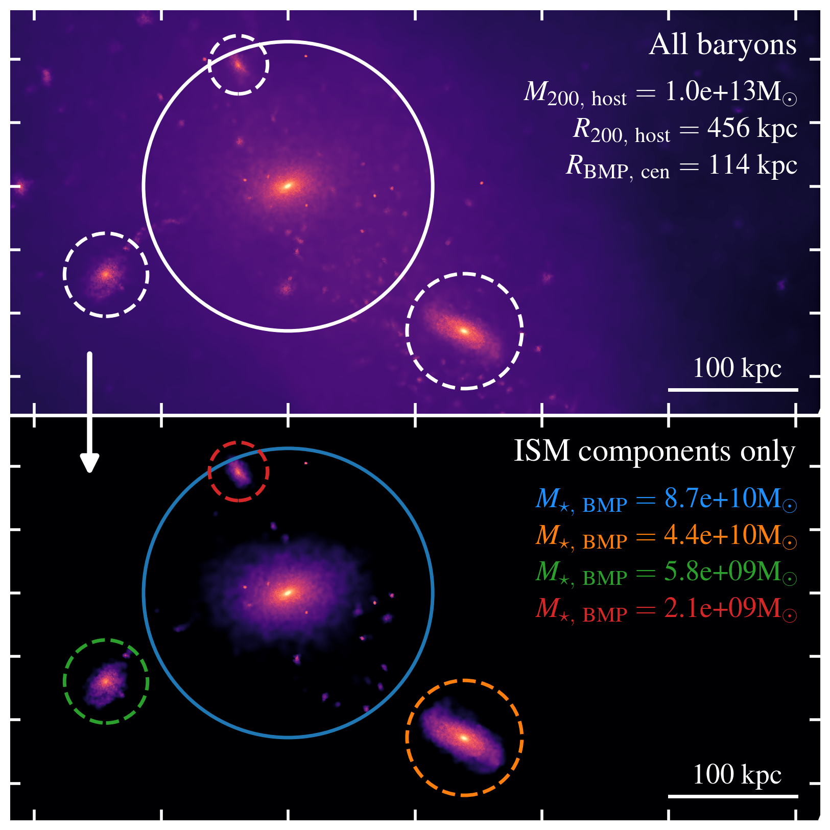
Figure 1: An illustration of our ISM selection process for a number of galaxies in a $\log(M_{\rm 200}/{\rm M_{\odot}})\$$\approx 13$ eagle halo at $z=0$. The top panel shows a rendering of all baryons, while the bottom panel solely exhibits the ISM selection. The BMP best-fit radii (Stevens et al., 2014) are illustrated with solid lines for the central galaxy, and dashed lines for the surrounding satellites. The stellar masses internal to each $R_{\rm BMP}$ are quoted in the bottom panel.

To summarise, for the remainder of the paper, we use the following terms when referring to different mass reservoirs and gas flow rates:

• Stellar mass ($M_{\star}$): the mass of stellar particles within $R_{\rm BMP}$;

• ISM mass ($M_{\rm ISM}$): the mass of cool ($T<5\times 10^{4}{\rm K}$ or ${\rm SFR}>0$) gas within $R_{\rm BMP}$, approximating a selection of the neutral phase;

• CGM mass ($M_{\rm CGM}$): the total mass of non-ISM gas associated with a subfind (sub)halo;

• Inflow & outflow rate ($\dot{M}_{\rm in}$ & $\dot{M}_{\rm out}$): the rate of gas mass entering or leaving the ISM, averaged over the interval of 2 snipshots;

• Star formation rate ($\dot{M}_{\star}$ or SFR): the mass of stars formed within $R_{\rm BMP}$, averaged over the interval of 2 snipshots;

• Halo mass ($M_{\rm 200}$): the total mass of a halo within the radius ($R_{\rm 200}$) that encloses an overdensity 200 times greater than the critical density of the universe in the simulation.

2.4 Generating an orbital catalogue with OrbWeaver

OrbWeaver is a tool used to extract orbital information from merger trees (Poulton, 2019; Poulton et al., 2020). It does this by identifying all satellites that come within a factor $N$ of their host virial radius ($R_{\rm vir,\ host}$). Using a root-finding algorithm, the exact timing of the desired $N\times R_{\rm vir,\ host}$ crossings and apsis points are determined. Once these points are found, interpolation is used to calculate the relative satellite-host properties and the associated satellite orbital parameters. Like our gas flow calculations, we ran OrbWeaver on the $200$-output eagle snipshot merger trees to identify and quantify the orbits of all satellites in the simulation. We remark that in this study, we do not focus on galaxies that have been “pre-processed” (i.e. those that enter a group/cluster environment already bound to a host). Rather, we seek to understand the physical processes that quench satellites on their first infall to a group environment.

3 The balance of gas flows in eagle central and satellite galaxies

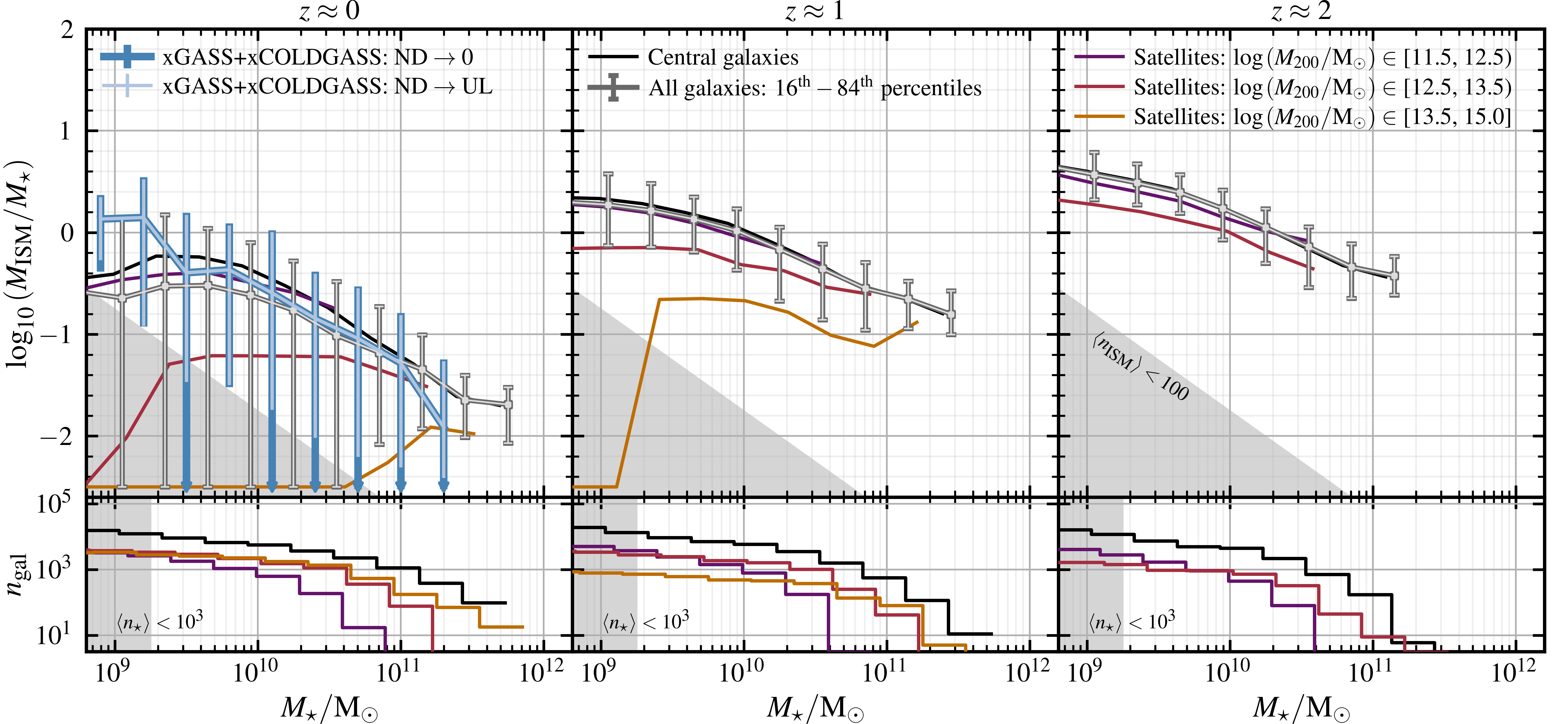
Figure 2: Comparison of the ISM gas mass ($T<5\times 10^{4}{\rm K}$ or ${\rm SFR}>0$) of eagle galaxies, binned by satellite halo mass. These gas masses are shown as a function of stellar mass, with 3 bins per decade in stellar mass. From left to right, results are shown including the $6$ snipshots closest to $z=0$, $z=1$ and $z=2$ respectively. In the left ($z\approx 0$) panel, we include a comparison to the xGASS+xCOLDGASS surveys (Saintonge et al. 2017; Catinella et al. 2018) in blue, with the range indicating $16^{\rm th}$-$84^{\rm th}$ percentiles, with non-detections assumed to be the lower percentile. We convert the summed H₂ and ${\rm H}$i content to equivalent ISM mass by assuming that $M_{\rm H_{2}}+M_{\rm HI}=M_{\rm ISM}/1.3$, where the factor of $1.3$ accounts for the abundance of Helium. In each panel, galaxies are classified as centrals (black) or satellites split into 3 bins of halo mass: (i)  sub-$L^{\star}$ haloes with $\log(M_{\rm 200}/{\rm M_{\odot}})\$$\in[11.5,12.5)$ (purple), (ii) group haloes with $\log(M_{\rm 200}/{\rm M_{\odot}})\$$\in[12.5,13.5)$ (red), and (iii) larger group/cluster haloes with $\log(M_{\rm 200}/{\rm M_{\odot}})\$$\in[13.5,15]$ (orange). The medians for all eagle galaxies are also indicated in grey. Error-bars display the $16^{\rm th}-84^{\rm th}$ percentile range in each stellar mass bin. Grey shaded regions in the top panels indicate the ISM mass that would correspond to 100 gas particles. The bottom panels illustrate the number of galaxies included in the top panels for each sample, with the grey regions indicating where the stellar mass of galaxies corresponds to less than $1000$ stellar particles.

In this section, we compare the gas mass, gas flow and star formation rates in central and satellite galaxies as a function of stellar mass and halo mass. In the context of the equilibrium model, the balance between these different different gas flows allows us to predict whether a galaxy is net gaining, maintaining, or losing gas mass from the ISM. While previous work has separately explored inflow and outflow rates in eagle galaxies (e.g. van de Voort et al. 2017; Correa et al. 2018b; Mitchell et al. 2020a, b), we aim to directly compare these flow rates together with star formation rates to explore the evolution of galaxy gas reservoirs as a function of galaxy environment. Specifically, we seek to understand the circumstances under which eagle galaxies net grow their ISM gas reservoir.

Schaye et al. (2015) show that convergence criterion relating to stellar mass functions and star formation rates are not met for eagle galaxies below $\approx 10^{9}{\rm M}_{\odot}$ in stellar mass. As such, we have chosen to remove these galaxies from our analyses in §3 and §4.

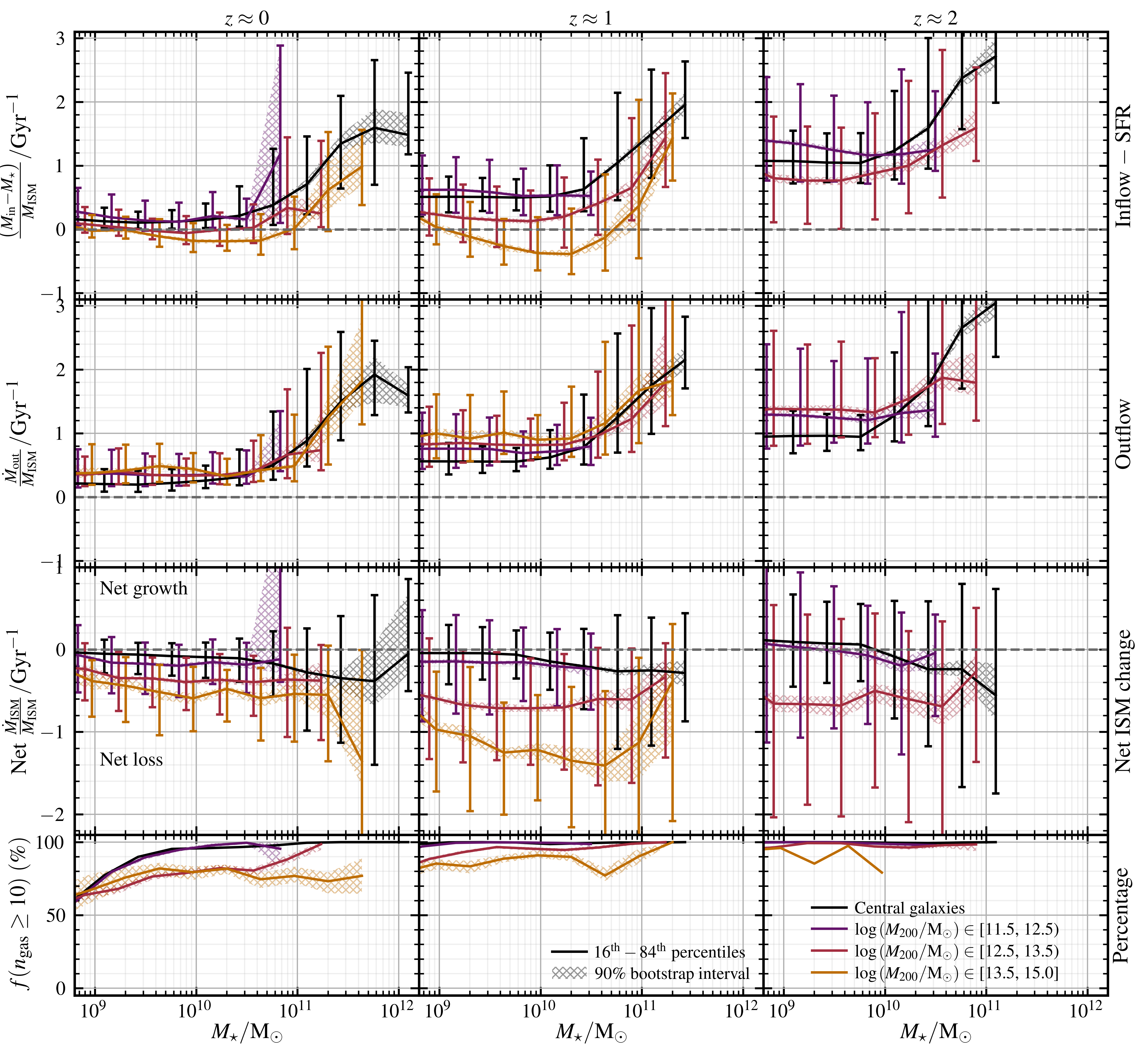
Figure 3: ISM inflow subtract star formation rates ($1^{\rm st}$ row), outflow rates ($2^{\rm nd}$ row), and net flow rates ($3^{\rm rd}$ row; sum of $1^{\rm st}$ and $2^{\rm nd}$ rows) in eagle galaxies, normalised by ISM mass. To ensure that the denominator is non-zero and that these specific flow rates are converged, only galaxies with 10 or more ISM gas particles ($M_{\rm ISM}\gtrsim 10^{7}{\rm M}_{\odot}$) are included in these calculations. The fraction of galaxies for which this criterion is met is illustrated in the bottom panels. Specific flow rates are shown as a function of stellar mass, with 3 bins per decade in stellar mass. From left to right, results are shown including the $6$ snipshots closest to $z=0$, $z=1$ and $z=2$ respectively. In each panel, galaxies are classified as centrals (black) or satellites split into 3 bins of halo mass: (i)  sub-$L^{\star}$ haloes with $\log(M_{\rm 200}/{\rm M_{\odot}})\$$\in[11.5,12.5)$ (purple), (ii) group haloes with $\log(M_{\rm 200}/{\rm M_{\odot}})\$$\in[12.5,13.5)$ (red), and (iii) larger group/cluster haloes with $\log(M_{\rm 200}/{\rm M_{\odot}})\$$\in[13.5,15]$ (orange). Error-bars display the $16^{\rm th}-84^{\rm th}$ percentile range in each stellar mass bin, and cross-hatched regions denote the bootstrap-generated $90\%$ confidence interval on the medians (based on 500 re-samples). We only include bins with at least 20 galaxies, and exclude any galaxies undergoing merger events from each of these samples.

Fig. 2 illustrates the ISM gas masses calculated for eagle galaxies at $z\approx 0$, $z\approx 1$, and $z\approx 2$, as per the method outlined in §2.3 and Appendix A. Each panel contains the results for $5$ samples: one for central galaxies of all halo mass (black), one for all central and satellite galaxies (grey), and 3 samples of satellites split into bins of halo mass: (i) sub-$L^{\star}$ haloes with $\log(M_{\rm 200}/{\rm M_{\odot}})\$$\in[11.5,12.5)$, (ii) group haloes with $\log(M_{\rm 200}/{\rm M_{\odot}})\$$\in[12.5,13.5)$ and (iii) larger group/cluster haloes with $\log(M_{\rm 200}/{\rm M_{\odot}})\$$\in[13.5,15]$. We use a larger bin width for the highest halo mass sample to ensure that we include the most massive haloes in the simulation.

The $1^{\rm st}$ row of panels in Fig. 2 illustrates the mass of gas in the ISM of eagle galaxies, as per the definition in §2.3 and Appendix A. In the left ($z\approx 0$) panel, we include a comparison to neutral hydrogen gas content measured the xGASS (extended GALEX Aricebo SDSS Survey; Catinella et al. 2018) & xCOLDGASS (extended CO Legacy Database for GASS; Saintonge et al. 2017) surveys, where non-detections have assumed to take the value of the lower percentile. We convert the summed H₂ and ${\rm H}$i content to equivalent ISM mass by assuming that $M_{\rm H_{2}}+M_{\rm HI}=M_{\rm ISM}/1.3$, where the factor of $1.3$ accounts for the abundance of Helium. We remark that these samples are mass-selected from SDSS, and reside in the redshift range $0.01<z<0.05$.

Firstly, we note that our measurements of ISM mass (for all galaxies) agree favourably with measurements from the xGASS/xCOLDGASS surveys for galaxies with stellar mass above $10^{9.5}{\rm M}_{\odot}$. Between $M_{\star}\approx 10^{9.5}{\rm M}_{\odot}-10^{11}{\rm M}_{\odot}$, our measurements of gas content are within $0.1-0.2$ dex of the xGASS/xCOLDGASS medians – giving us confidence in our ISM classification. The two xGASS/xCOLDGASS data-points at stellar mass below $10^{9.5}{\rm M}_{\odot}$ suggest that our measurements of ISM mass may under-predict the gas content of low-mass galaxies relative to observations. We remark that this may be related to numerical issues in eagle, with galaxies in this mass range having just $\approx 100$ gas particles on average.

As demonstrated previously in both observations (e.g. stellar mass – ${\rm H}$i mass relation in Brown et al. 2017; Calette et al. 2021) and cosmological simulations (e.g. Bahé et al. 2016; Stevens et al. 2019), we find that at fixed stellar mass, satellites residing in more massive host haloes have lower cool gas content. For satellites in the lowest halo mass sample – $\log(M_{\rm 200}/{\rm M_{\odot}})\$$\in[11.5,12.5)$ – the reduction in gas content relative to centrals is small; only $0.1-0.2$ dex across all stellar mass and redshift. The reduction in gas content in the satellite samples is more dramatic for the small group-mass sample and large group/cluster-mass sample – with only galaxies above $10^{10.5}{\rm M}_{\odot}$ ($10^{9}{\rm M}_{\odot}$) in the large group/cluster (small group) sample showing ISM gas masses above the floor value at $z\approx 0$.

In Fig. 3, we illustrate the gas flow rates relating to the ISM eagle galaxies (as per §2.3 & 2.3) normalised by ISM mass as a function of stellar mass. These “specific” flow rates, as opposed to total flow rates, reflect the magnitude of influence that the gas flows and star formation will have on the galaxy. For measurements of total inflow rates to eagle satellites, we refer the reader to van de Voort et al. (2017) – who find clear environmental suppression of total gas accretion rates to eagle satellites.

The remaining samples of low-mass $z<1$ satellites in groups/clusters reflects those that have not yet been completely stripped of their cool gas, which as we demonstrate in §4, are likely the satellites that are on first-infall to the host. We stress that the galaxies remaining in the sample are not atypical, as the vast majority of central galaxies – reflecting the expected behaviour of satellites pre-infall – meet this criterion. We note that the majority of satellite infall events occur between $z\approx 0.5$ and $z\approx 1.5$ (see §4), and thus focus a large proportion of our discussion on the $z\approx 1$ sample.

The $1^{\rm st}$ row of panels in Fig. 3 illustrates median ISM inflow rates, subtract SFRs, normalised by ISM mass (which we refer to as “specific replenishment rate”). This quantity is a measure of the imbalance between star formation and fresh gas accretion — i.e., whether the current rate of gas inflow is adequate to sustain the current star formation rate. At $z\approx 1$, the environmentally-driven suppression in gas accretion relative to SFR in satellites becomes evident. This is illustrated in the relative normalisation of the curves for satellites in different halo mass bins, and is particularly notable for galaxies in larger clusters/groups.

At $z\approx 1$, central galaxies maintain a steady median value of $(\dot{M}_{\rm in}-\dot{M}_{\star})/{M_{\rm ISM}}\approx 0.3\ {\rm Gyr}^{-1}$ up to $\log(M_{\star}/{\rm M_{\odot}})\$$\approx 11$; with satellites in the lowest halo mass sample demonstrating very similar behaviour. Satellites with $\log(M_{\rm 200}/{\rm M_{\odot}})\$$\in[12.5,13.5)$ show specific replenishment rates offset negatively from centrals by $\approx 0.2$ ${\rm Gyr}^{-1}$, maintaining a value of $(\dot{M}_{\rm in}-\dot{M}_{\star})/{M_{\rm ISM}}\approx 0.1\ {\rm Gyr}^{-1}$ up to $\log(M_{\star}/{\rm M_{\odot}})\$$\approx 10.5$. While it is clear that suppression of gas accretion rates occurs in $\log(M_{\rm 200}/{\rm M_{\odot}})\$$\in[12.5,13.5)$ satellites relative to central galaxies, given that this median value remains positive, we conclude that the average satellite in this sample could not quench in the absence of outflows.

Such is not the case for satellites in the large group/cluster sample, $\log(M_{\rm 200}/{\rm M_{\odot}})\$$\in[13.5,15]$. These satellites show a clear dip in replenishment rates between $\log(M_{\star}/{\rm M_{\odot}})\$$=9-11$; with a value of $(\dot{M}_{\rm in}-\dot{M}_{\star})/{M_{\rm ISM}}\approx-0.5\ {\rm Gyr}^{-1}$ at $\log(M_{\star}/{\rm M_{\odot}})\$$\approx 10$. Assuming that these specific flow rates remain constant, full ISM depletion of the average satellite in this sample would occur in $\approx 2$ Gyr – even in the absence of outflows. We note that the magnitude of suppression of specific replenishment rates in $z\approx 0$ satellites relative to $z\approx 1$ galaxies is roughly halved, at $(\dot{M}_{\rm in}-\dot{M}_{\star})/{M_{\rm ISM}}\approx-0.25\ {\rm Gyr}^{-1}$ in the most extreme cases.

The $2^{\rm nd}$ row of panels in Fig. 3 show ISM outflow rates normalised by ISM gas mass (“specific outflow rates”). We find that specific outflow rates in satellite galaxies clearly increase with increasing halo mass – which is not the case if existing ISM mass is not controlled for. This picture aligns with the expectation of increased ram-pressure and tidal stripping in group environments. We stress that we do not distinguish between different gas removal mechanisms – but we remind the reader of the findings of Bahé & McCarthy (2015), who show that the majority of excess gas removal in satellites relative to field galaxies can be explained by ram pressure stripping, with a sub-dominant contribution from tidal stripping.

On average, outflow rates in satellite galaxies for all halo mass bins exceed those measured for central galaxies, with the exception of satellites with stellar mass $\log(M_{\star}/{\rm M_{\odot}})\$$>11$. At $z\approx 1$, central galaxies exhibit fairly constant specific outflow rates at $\dot{M}_{\rm out}/M_{\rm ISM}\approx 0.4\ {\rm Gyr}^{-1}$ in galaxies below $\log(M_{\star}/{\rm M_{\odot}})\$$\approx 11$, effectively balancing specific replenishment rates. All satellite samples show steadily increasing specific outflow rates with halo mass – with $\dot{M}_{\rm out}/M_{\rm ISM}$ values of $0.5\ {\rm Gyr}^{-1}$, $0.75\ {\rm Gyr}^{-1}$, and $1\ {\rm Gyr}^{-1}$ for the three halo mass samples from $\log(M_{\rm 200}/{\rm M_{\odot}})\$$=11.5$ to $\log(M_{\rm 200}/{\rm M_{\odot}})\$$=15$ respectively. For satellites in the large group/cluster-mass bin, this means that in the absence of star formation and inflows, such galaxies would have their full gas reservoir stripped within $1$ Gyr.

Adding the quantities in the $1^{\rm st}$ and $2^{\rm nd}$ rows of panels, we illustrate the total net rate of change in ISM mass of galaxies in the $3^{\rm rd}$ row of panels. This quantity reflects the deviation of a galaxy from being in equilibrium – with a net positive rate meaning that a galaxy would be expected to build up its ISM gas reservoir; and a net negative value meaning a galaxy would be net depleting its ISM reservoir. As per Equation 3, these net flow rates correspond to the inverse of the predicted depletion time-scale of the ISM, assuming that the flow rates remain constant. For all epochs shown, central galaxies generally show net flow values very close to equilibrium below $\log(M_{\star}/{\rm M_{\odot}})\$$\approx 11$. This is also true for satellite galaxies in the  sub-$L^{\star}$ halo mass sample. In the two more massive halo mass samples, however, it is clear to see the combined influence of stripping and starvation on satellites – particularly at $z\approx 1$.

Focusing on the small group-mass sample, $\log(M_{\rm 200}/{\rm M_{\odot}})\$$\in[12.5,13.5)$ – we record net $\dot{M}_{\rm ISM}/M_{\rm ISM}$ values of $\approx-0.6\ {\rm Gyr}^{-1}$ – corresponding to an average depletion time of $\approx 1.5$ Gyr (assuming the net specific flow rate remains constant); this value remaining relatively steady over stellar mass up to $\log(M_{\star}/{\rm M_{\odot}})\$$\approx 11$. If one were to assume that these satellites experienced the same specific replenishment as central galaxies; this would shift $\dot{M}_{\rm ISM}/M_{\rm ISM}$ values from $-0.6\ {\rm Gyr}^{-1}$ to $\approx-0.3-0.4\ {\rm Gyr}^{-1}$ – corresponding to depletion times of $\approx 2.5-3$ Gyr on average. Thus, even though these galaxies do not experience sufficient suppression in gas accretion to quench via starvation alone (as per the positive specific replenishment rates), the moderate reduction in specific inflow rates can accelerate the depletion of ISM reservoirs by a factor of $\approx 2$ on average.

Focusing on the large group/cluster-mass sample, $\log(M_{\rm 200}/{\rm M_{\odot}})\$$\in[13.5,15]$ at $z\approx 1$ – we note mild variation in $\dot{M}_{\rm ISM}/M_{\rm ISM}$ across stellar mass. Satellites at $\log(M_{\star}/{\rm M_{\odot}})\$$=9$ and $\log(M_{\star}/{\rm M_{\odot}})\$$=11$ see a net value of $\dot{M}_{\rm ISM}/M_{\rm ISM}\approx-1\ {\rm Gyr}^{-1}$, but between these mass scales, there is a slight peak in the net loss rate at $\log(M_{\star}/{\rm M_{\odot}})\$$=10$, at $\dot{M}_{\rm ISM}/M_{\rm ISM}\approx-1.4\ {\rm Gyr}^{-1}$ (corresponding to a depletion time of $\approx 0.7\ {\rm Gyr}$, assuming a constant specific outflow rate). This reflects the peak suppression of specific replenishment rates at this mass scale, where SFRs clearly exceed near-zero inflow rates. Assuming that such a satellite were to experience the same specific replenishment rates as centrals, the same net value of $\dot{M}_{\rm ISM}/M_{\rm ISM}$ would shift to $\approx-0.8\ {\rm Gyr}^{-1}$ – that is to say, the same rate of stripping would be capable of completely depleting the ISM of a central galaxy (in the absence of starvation) within $\approx 1.2\ {\rm Gyr}$. Assuming a net balance between star formation and inflows and a constant specific outflow rate, outflows alone would deplete the ISM in $\approx 1\ {\rm Gyr}^{-1}$.

In general, we note that that there is notably increased $16{\rm th}-84^{\rm th}$ percentile spread in gas inflow, outflow, and net flow rates with increasing redshift. Given that these quantities are actually better sampled at higher redshift (due to systematically higher gas flow rates at early times), we argue that this increased variance is a true reflection of a galaxy population exhibiting real diversity in terms of evolutionary pathways.

In the most extreme examples of starvation – $\log(M_{\star}/{\rm M_{\odot}})\$$\approx 10$ satellites in groups with $\log(M_{\rm 200}/{\rm M_{\odot}})\$$>13.5$ at $z=1$ – galaxies experience a median offset between inflow and SFR of $(\dot{M}_{\rm in}-\dot{M}_{\star})/M_{\rm ISM}\approx-0.4\ {\rm Gyr}^{-1}$. Assuming an outflow rate that matches the average central galaxy of the same mass, $\dot{M}_{\rm out}/M_{\rm ISM}\approx 0.5\ {\rm Gyr}^{-1}$, the net (negative) specific flow rate does not exceed $\dot{M}_{\rm net}/M_{\rm ISM}=1\ {\rm Gyr}^{-1}$. This means that even in the most extreme cases of starvation, at least 50% of satellites will still require enhanced outflows (i.e., direct cold gas stripping) to produce sub-Gyr indicative depletion time-scales. Such depletion time-scales can be produced by stripping alone. However, this does not preclude the occurrence of starvation, which can moderately accelerate the process.

Table 2: Different gas flow classifications based on average inflow, outflow, and SFRs. We class galaxies into those that are (a) net growing or maintaining their ISM reservoir, (b) slowly depleting their ISM reservoir, (c) rapidly depleting their ISM reservoir, and (d) quenched. The delineating depletion time-scale between “slow” and ”rapid” quenching is 1.5 Gyr, based on the median quenching time-scale ($\tau_{\rm Q}$) value measured for eagle galaxies in Wright et al. (2019). The shading used for the histograms in Figs. 4 and 8 is provided in the right-hand column.

With information about a galaxy’s ISM mass, and its inflow, outflow and star formation rates (as presented in 3) – we can predict the mass of gas in the ISM of a galaxy at a time $t+\Delta t$ if we take Equation 1 and discretise in time:

$$M_{\rm ISM}(t+\Delta t)=M_{\rm ISM}(t)+[\dot{M}_{\rm in}(t)-\dot{M}_{\rm out}(t)-\dot{M}_{\star}(t)]\times\Delta t.$$ (2)

If the quantity in the square brackets (inflow rate subtract outflow rate and star formation rate) is negative – the ISM is being net depleted, and we can calculate an indicative depletion time-scale by setting $M_{\rm ISM}(t+\Delta t)$ to $0$, solving for $\Delta t$:

$$\Delta t\equiv T_{\rm dep}=\frac{M_{\rm ISM}}{\dot{M}_{\rm in}-\dot{M}_{\rm out}-\dot{M}_{\star}}=\frac{M_{\rm ISM}}{{\rm Net}\ \dot{M}_{\rm ISM}};$$ (3)

where a net flow rate of $\dot{M}_{\rm ISM}/M_{\rm ISM}=\pm 1$ corresponds to a galaxy in which the flow rate would add (remove) the present gas mass of the ISM in 1 Gyr. We stress that this parameterisation of $T_{\rm dep}$ corresponds to an indicative depletion time-scale, and makes the assumption that inflow, outflow, and star-formation rates remain constant. We also remark that we do not include the return of gas to the ISM via stellar winds in this calculation, however, have confirmed that this is a very minimal effect and seldom influences our conclusions.

Building on the arguments presented above regarding net flow rates and depletion time-scales, it is possible to classify the evolutionary state of a galaxy into one of four categories, as outlined in Table 2. Galaxies can either be (a) net growing or maintaining their ISM reservoir, (b) slowly depleting their ISM reservoir, (c) rapidly depleting their ISM reservoir, or (d) quenched. Galaxies in which the inflow rate exceeds the sum of outflow rate and SFR are classified into (a), as are those that have a depletion time-scale greater than $10$ Gyr. Galaxies with ISM depletion time-scales between $1.5-10$ Gyr are classified as “slowly” depleting, while those with depletion time-scales less than $1.5$ Gyr are classified as “rapidly” depleting. We use $1.5$ Gyr as the delineating time-scale based on the median quenching time-scale ($\tau_{\rm Q}$) value measured for eagle satellite galaxies in Wright et al. (2019) defined by sSFR, though remark our results are qualitatively insensitive to this choice for values between $1$ and $4$ Gyr.

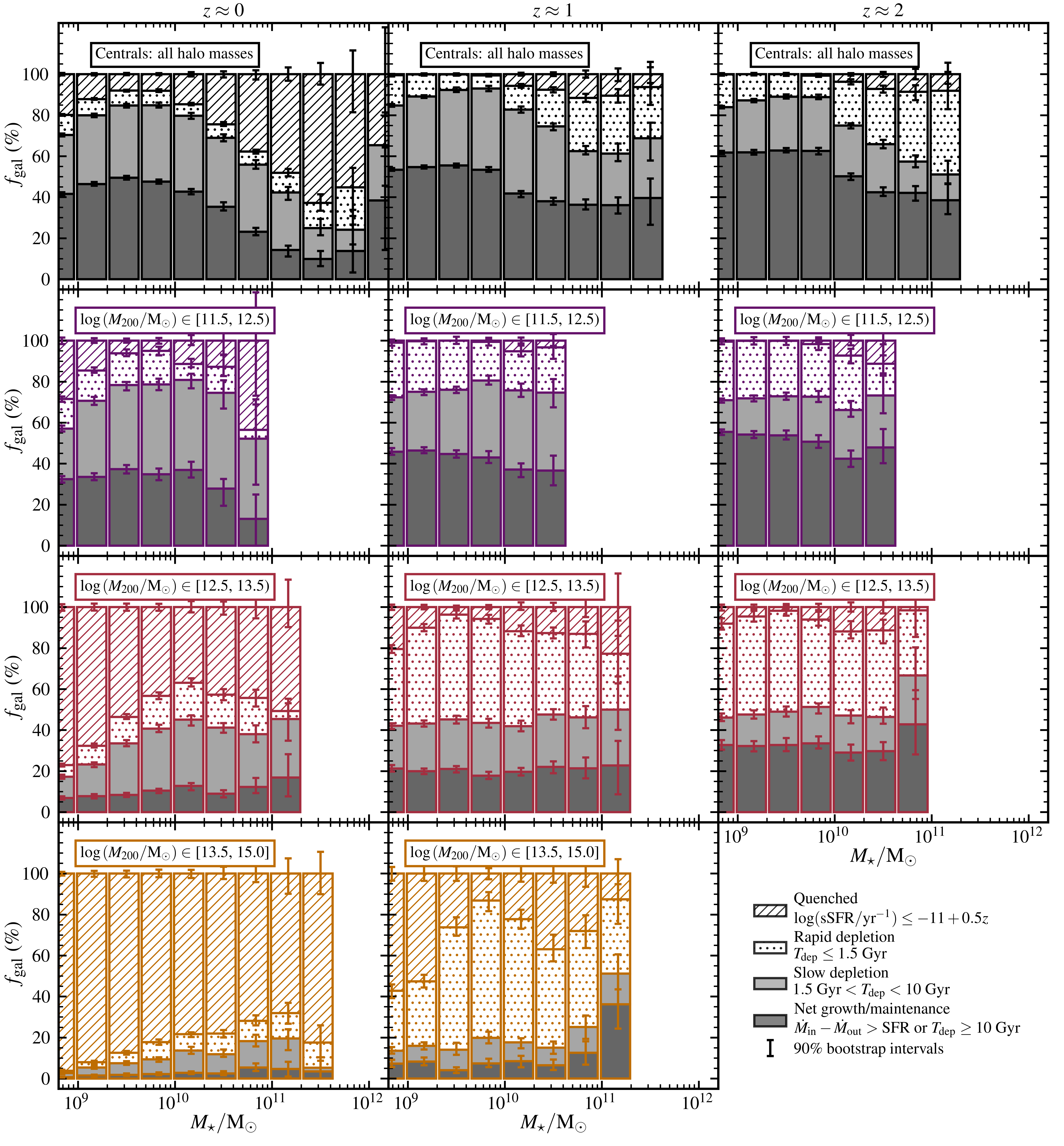
Figure 4: The breakdown of galaxies into gas flow classes (outlined in Table 2), as a function of stellar mass (with 3 bins taken per decade in mass). A galaxy can be classified as either (a) net growing/maintaining its ISM reservoir – dark grey shading; (b) slowly depleting its ISM reservoir – light grey shading; (c) rapidly depleting its ISM reservoir – dotted shading; and (d) quenched – forward-hatched shading. The delineating time-scale between “slow” and ”rapid” depletion is $1.5$ Gyr, based on the median quenching time-scale ($\tau_{\rm Q}$) value measured for eagle galaxies in Wright et al. (2019). Each column corresponds to a different epoch; including the $6$ snipshots closest to $z=0$, $z=1$ and $z=2$ from left to right. Each row corresponds to a different sample, with the top panels illustrating the breakdown for central galaxies, and the bottom $3$ rows showing the results for satellite galaxies in bins of increasing halo mass. We only include stellar mass bins where the statistics have been calculated with at least 20 galaxies. We do not include the results for satellites in the highest halo mass bin at $z\approx 2$ due to low number statistics. Error-bars denote the bootstrap-generated $90\%$ confidence interval on the fractions (based on 500 re-samples). We exclude galaxies undergoing a major or minor merger from each of these samples.

As per the discussion in §1, a galaxy experiencing reduced accretion rates and “slow” quenching would closely reflect the archetypal starvation scenario, compared to a galaxy experiencing “fast” quenching that closely reflects a “stripping” scenario. Our results above suggest that significant stripping is certainly required to produce $<{\rm Gyr}$ quenching time-scales, however does not preclude the suppression of gas accretion taking place. We also note that the indicative depletion time-scale of a galaxy based on instantaneous flow rates, in some cases, may systematically under-predict the time it takes to deplete a galaxy’s ISM reservoir. This is because the rate of gas removal via both stripping and consumption in star formation are likely to scale down with the decreasing gas content of the ISM (and not remain at the initial high removal rates), and prolong the quenching phase.

We classify galaxies as “quenched” (i.e., depleted) if they meet the simple criteria $\log({\rm sSFR}/{\rm yr}^{-1})<-11+0.5z$ (e.g. Furlong et al. 2015), and do not otherwise meet the criteria to be classified into group (a). Our choice to exclude “rejuvenating” galaxies from the quenched population means that group (d) does not exactly correspond to a classically defined “quenched fraction”, however we remark that the proportion of rejuvenating galaxies in the samples considered is ubiquitously very low ($<1\%$). We also remark that our quenched definition, being based on sSFR, does not explicitly ensure that the ISM of a galaxy has been entirely depleted. Pragmatically, however, we have found that this cut seldom selects galaxies with gas fractions above $0.05$, and importantly allows us to determine the “quenched” status of galaxies with a commonly used observable property.

Using the arguments above, Fig. 4 shows the fraction of galaxies belonging to the gas flow classes outlined in Table 2 as a function of stellar mass at $z\approx 0$, $z\approx 1$, and $z\approx 2$. We split the sample of galaxies into the same selections illustrated in Figs. 2 and 3; namely, centrals of all halo masses, and satellites in $3$ bins of halo mass between $\log(M_{\rm 200}/{\rm M_{\odot}})\$$=11.5$ and $15$.

Focusing first on central galaxies (top row), we note that the fraction of galaxies able to maintain or grow their ISM reservoir decreases with stellar mass. At $z\approx 2$ the fraction of galaxies growing or maintaining their ISM sits at $60-65\%$ for galaxies with stellar mass below $\log(M_{\star}/{\rm M_{\odot}})\$$=10$, with the ISM of approximately $20-30\%$ of galaxies classified as slowly depleting in the same mass range. For galaxies above $\log(M_{\star}/{\rm M_{\odot}})\$$=10$ at $z\approx 2$, the fraction drops towards $40\%$, with a much higher proportion of galaxies ($\approx 30\%$) experiencing rapid depletion. This is likely due to AGN feedback in this stellar mass range. Instead considering $z\approx 0$ galaxies, $40-50\%$ of centrals are net growing their ISM reservoir below $\log(M_{\star}/{\rm M_{\odot}})\$$\approx 10$, and above this mass, the quenched fraction increases to $\approx 60-70\%$. Aside from high-mass galaxies at $z\approx 2$, it appears that there are ubiquitously more centrals in the slowly depleting group compared to the rapidly depleting group. This aligns with the quenching time-scales found in Wright et al. (2019), who show that very few centrals quench in time-scales shorter than $\approx 1$ Gyr.

The behaviour of satellites in the lowest halo mass sample, $\log(M_{\rm 200}/{\rm M_{\odot}})\$$\in[11.5,12.5)$ (second row), is very similar to the sample of central galaxies, with only very slight increases in the proportion of rapidly-quenching galaxies. This is true up to $\log(M_{\star}/{\rm M_{\odot}})\$$\approx 11$ at $z\approx 0$, as very few satellites exist above this stellar mass in this sample. Galaxies in the next halo mass sample, $\log(M_{\rm 200}/{\rm M_{\odot}})\$$\in[12.5,13.5)$ (third row), begin to show the clear signatures of environmentally-induced quenching. At $z\approx 2$, just over $50\%$ of $\log(M_{\star}/{\rm M_{\odot}})\$$<10.5$ satellite galaxies in this sample exist in the rapidly depleting group – much higher than the slowly depleting fraction at $\approx 10-20\%$. The quenched fraction grows correspondingly towards $z\approx 0$, with the fraction of satellites quenched largest ($>50\%$) for $\log(M_{\star}/{\rm M_{\odot}})\$$<9.5$ (due to environmental effects) and $\log(M_{\star}/{\rm M_{\odot}})\$$>11$ (due to AGN feedback).

Galaxies in the highest halo mass bin, $\log(M_{\rm 200}/{\rm M_{\odot}})\$$\in[13.5,15]$ (bottom row), corresponding to larger groups and clusters, show even more dramatic signatures of environmental quenching, with $\approx 80\%$ of the non-quenched sample at $\log(M_{\star}/{\rm M_{\odot}})\$$\approx 10$ experiencing rapid ISM depletion. Very few satellites in this sample are able to net grow or maintain their ISM reservoir: $\approx 5\%$ at $z\approx 1$, and even less at $z\approx 0$. At $z\approx 0$, we measure that approximately $80\%$ of satellites are quenched (averaged across stellar mass), with the fraction highest for galaxies with $\log(M_{\star}/{\rm M_{\odot}})\$$<9.5$. As we show in §4, the small fraction of un-quenched satellites in this sample is likely a reflection of the population of satellites that have not yet entered the host’s virial radius.

4 Gas flows along the infall and orbit of satellite galaxies

In this section, we move from the static analysis of §3 to a temporal analysis of the gas mass, flow rates and star formation rates in satellite galaxies along their infall and orbits in group and cluster environments. We again stress that while previous work has separately explored inflow, outflow and star formation rates in satellite galaxies, we aim to holistically consider these processes and their combined role in regulating the gas content of satellite galaxies.

To identify the infall and orbits of satellites in eagle, we make use of the OrbWeaver tool as described in §2.4 (Poulton, 2019; Poulton et al., 2020). In the case where multiple orbital hosts for a single galaxy have been identified, we only consider the most massive host. We then select galaxies for our orbital analysis by applying the following criteria at the first pericentric passage (fp) for each galaxy (and quote the percentage of fps for which this criterion is met):

• $z_{\rm fp}\leq 2$ ($93.9\%$) – ensures that particle data is available;

• Host $\log(M_{\rm 200}/{\rm M_{\odot}})\$$\geq 12.5$ ($54.2\%$) – expect significant environmental effects;

• Satellite $\log(M_{\star}/{\rm M_{\odot}})\$$\in[8,11]$ ($94.6\%$) – removes very small and very massive satellites;

• Orbital radius within $R_{\rm 200}$ of host ($57.2\%$) – consider only close approaches.

This extracts a total of $7\ 803$ first pericentric passages in the eagle L100-REF box. We do not include satellites with a (pericentric) stellar mass above $10^{11}{\rm M}_{\odot}$ as there are very few, and in these circumstances the central-satellite delineation can be confused between outputs (e.g. Cañas et al. 2019). For the purposes of our analysis, we also require that each satellite reaches at least one apocenter post-infall, and that it is not lost in the merger trees prior to this point – reducing the sample to $2\ 810$ orbits. This reduction in sample size is due to several factors. Firstly, some satellites are disrupted prior to apocenter (i.e. destroyed, or merged with the host central). Secondly, given the high-density environment and interactions between haloes, the merger trees may struggle to match haloes across snapshots. Thirdly, many ($\approx 2\ 000$) of the orbits removed were recent infalls, with pericenters at lookback times of $\leq 1$ Gyr – meaning these galaxies were not necessarily expected to reach an apocenter by $z=0$. We do not include these late-infall galaxies in our sample, meaning our analysis is slightly biased to higher-redshift infall events (as explicitly shown in Fig. 6).

Lastly, we remove the satellites that have been “pre-processed” (i.e., have been a satellite in a host halo with $M_{200}>10^{12}{\rm M}_{\odot}$) prior to entering the current orbital host. This allows us to analyse how environment affects satellites on their first-infall to a group environment, and reduces our final sample to $2\ 054$ orbits. This pre-processed fraction, $\approx 30\%$, is slightly lower than that found previously by Bahé et al. (2019) using the Hydrangea simulations, with fractions typically above $50\%$ (aside from higher mass satellites in smaller groups). We note, however, that we only consider pre-processing to have occurred if the previous host was above a mass of $10^{12}{\rm M}_{\odot}$. Below this halo mass, based on the results presented in §3 and Fig. 4 (considering the lowest halo mass sample), we argue that the influence of environment is small due to the similarity between the properties of this sample of satellites and the sample of central galaxies. In addition, Hydrangea corresponds to cluster zooms and as such are biased to high density environments, where more pre-processing is expected, compared to the eagle box.

With the orbital characteristics of our sample generated with OrbWeaver, we are able measure an orbital time-scale and thus meaningfully analyse how the properties of the satellite change as a function of orbital time and phase.

4.1 Individual examples of satellite infall to groups in eagle

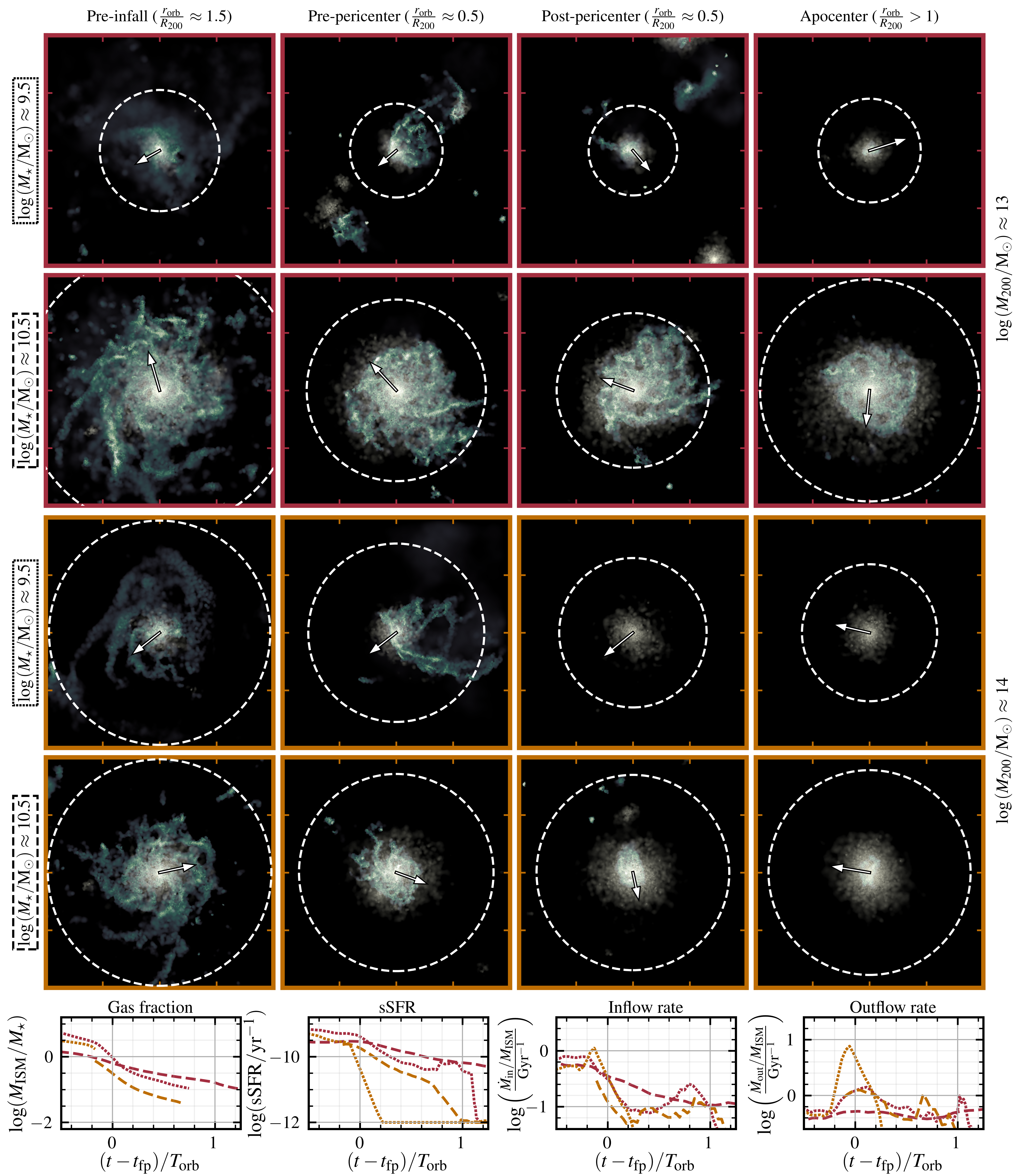
Figure 5: Example visualisations of satellites on their infall to group and cluster-mass haloes. Each row corresponds to the evolution of a single galaxy, tracked through the merger trees along its orbit. The top two rows of visualisation panels show example galaxies falling onto groups with mass $\log(M_{\rm 200}/{\rm M_{\odot}})\$$\in[12.5,13.5)$, and the bottom two rows of visualisation panels show galaxies falling into groups with mass $\log(M_{\rm 200}/{\rm M_{\odot}})\$$\in[13.5,15]$. The first and third rows of panels correspond to example galaxies at $\log(M_{\star}/{\rm M_{\odot}})\$$\approx 9.5$ (dotted lines in bottom panels) at first pericenter; while the second and fourth rows correspond to example galaxies at $\log(M_{\star}/{\rm M_{\odot}})\$$\approx 10.5$ (dashed lines in bottom panels). We remark that the stellar mass of these galaxies do not markedly change post-infall. From left to right, we include a visualisation of the satellite (i) pre-infall at $r_{\rm orb}/R_{200}=1.5$, (ii) pre-pericenter $r_{\rm orb}/R_{200}=0.5$, (iii) post-pericenter $r_{\rm orb}/R_{200}=0.5$, and (iv) at first apocenter. Axes ticks correspond to increments of $20$ pkpc. Stellar mass density and gas mass density are shown in pale yellow and green respectively, using the same logarithmic scaling. The velocity vector of the satellite’s center of mass and its relative magnitude in the image plane are included at the center of each panel; and the effective baryonic radii of the galaxies, $R_{\rm BMP}$, is illustrated with dashed lines. The bottom row of panels illustrates different properties of the satellites along their orbit, namely (from left to right): gas fraction, specific star formation rate, ISM inflow rate, and ISM outflow rate.

For illustrative purposes, we include example visualisations of the infall of a number of satellites part of our sample in Fig. 5. Each row of visualisation panels shows the same satellite along its orbit, from left to right: pre-infall ($\approx 1.5R_{200}$), pre-pericenter ($\approx 0.5R_{200}$), post-pericenter ($\approx 0.5R_{200}$), and at first apocenter ($>R_{200}$). The $4$ panels at the bottom of Fig. 5 illustrate the gas fractions, sSFRs, inflow rates, and outflow rates of each of the satellites shown.

We first focus on the top row of panels – an $M_{\star}\approx 10^{9.5}{\rm M}_{\odot}$ satellite on infall to a $M_{200}\approx 10^{13}{\rm M}_{\odot}$ halo. Pre-infall, the galaxy has a gas fraction (gas mass normalised by total baryonic mass) of $\approx 0.8$, an ${\rm sSFR}$ of $\approx 10^{-9}\ {\rm yr}^{-1}$, and its ISM inflow rate exceeds the outflow rate. Prior to pericenter, the radial extend of the galaxy’s gaseous component appears to exceed that of the stellar component. Once the galaxy enters $R_{\rm 200}$ in the second panel, there is evidence of a clearly disturbed gas morphology and a ram-pressure stripping tail opposite to the infall velocity vector. By this point, the galaxy’s gas fraction has begun to drop steeply; however the ${\rm sSFR}$ appears to only gradually reduce, even seeing a slight peak prior to pericenter as the gaseous leading edge of the galaxy is compressed by interaction with the intra-group medium. This agrees with the findings of Troncoso-Iribarren et al. (2020), who found using the eagle simulations that the leading half of satellite galaxies (as defined by the trajectory of the galaxy in the halo) in high mass groups has a higher ISM pressure than the trailing half – consistent with this observed compression.

Post-pericenter, the galaxy’s gas fraction visibly drops (to $\approx 0.25$), and the ${\rm sSFR}$ begins to show a steeper decline. Inflow rates drop by $\approx 1$ dex, while the outflow rate peaks close to pericenter, $\approx 0.5$ dex above the pre-infall value. At first apocenter, there is very little gas remaining in the galaxy (though not zero, as per the gas fraction panel), and the ${\rm sSFR}$ continues to steadily drop. Outflow rates decrease back to just above pre-infall values, however inflow rates remain very low – $\approx 1$ dex below pre-infall. After one pericentric passage, we note that the radial extent of the gaseous disk has contracted to roughly match the extent of the stellar disk.

The second row of panels shows a more massive $M_{\star}\approx 10^{10.5}{\rm M}_{\odot}$ galaxy on infall to a similar mass, $M_{200}\approx 10^{13}{\rm M}_{\odot}$ halo. Pre-infall (at $\approx 1.5R_{\rm 200}$), the galaxy has a gas fraction and sSFR slightly lower than its lower mass counterpart at $\approx 0.6$, consistent with the global mass – sSFR relation. When the galaxy enters $R_{\rm 200}$, we can see the gaseous component of the galaxy becomes slightly compressed on the leading edge of the disk, and slightly extended in the trailing direction. The rate of sSFR decline remains relatively steady on infall though, and outflow rates show a very slight increase around pericenter, $\approx 0.1-0.2$ dex above pre-infall values. After pericenter, we note a steeper decrease in galaxy gas fraction, and that the reduction in ${\rm sSFR}$ begins to accelerate again. Inflow rates steadily drop after pericenter to $\approx 0.5$ dex below pre-infall values at apocenter, where the galaxy’s gas fraction has dropped to $\approx 0.3$. While environment has a clear influence on the quenching of this galaxy, the decline in sSFR and gas fraction is relatively gentle, driven primarily by consumption of existing gas (starvation) after entry to the halo. Helping this gentle decrease in SFR is the lack of strongly enhanced outflow rates after pericenter.

The third row of panels illustrates an $M_{\star}\approx 10^{9.5}{\rm M}_{\odot}$ satellite on infall to a more massive, $M_{200}\approx 10^{14}{\rm M}_{\odot}$ halo. Pre-infall, the galaxy has a gas fraction and sSFR ($\approx 0.8$ and $\approx 10^{-9}\ {\rm Gyr}^{-1}$ respectively) similar to the galaxy of roughly equal mass in the top row of panels. Additionally, the inflow rate at $(t-t_{\rm fp})/T_{\rm orb}\approx-1$ of $\approx 10^{0}\ {\rm Gyr}^{-1}$ clearly exceeds the outflow rate, $\approx 10^{-0.3}\ {\rm Gyr}^{-1}$. In the first visualisation panel, the galaxy shows little visual sign of disturbance on its infall. In the second panel, pre-pericenter, we see a very clearly disturbed gas morphology, with gas heavily compressed on the leading edge of the galaxy and extended in the trailing direction. This is reflected in massively increased outflow rates, peaking at $\approx 10^{1}\ {\rm Gyr}^{-1}$ at pericenter – which would correspond to complete removal of the cold gas reservoir within $100\ {\rm Myr}$, even in the absence of star formation. In the third panel, we can clearly see that there is no gas remaining – with sSFR and gas fractions dropping near to zero very shortly after pericentric passage. After first pericenter, we also note that inflow rates to the ISM remain below $\approx 10^{-1}\ {\rm Gyr}^{-1}$, meaning there is very little change for rejuvenation.

Lastly, the fourth row of panels illustrates an $M_{\star}\approx 10^{10.5}{\rm M}_{\odot}$ satellite on infall to an $M_{200}\approx 10^{14}{\rm M}_{\odot}$ halo. In the first panel, we observe a clear disk-like morphology, with the galaxy’s gaseous component extending radially further than the more compact stellar component. The galaxy shows a similar pre-infall gas fraction and sSFR ($\approx 0.6$ and $\approx 10^{-9.5}\ {\rm Gyr}^{-1}$ respectively) to its equal-mass counterpart in the second row of panels. In this large host, however, this gas fraction and sSFR actually begin to drop even prior to pericenter – as reflected in the second panel where the outer gas disk has been stripped to roughly match the radial extent of the stellar component. Post-pericenter, in the third panel, we observe even more gas removal – with a clearly disturbed gas morphology embedded in the mostly undisturbed stellar disk. While a large amount of gas has been removed, the gas content of the galaxy does not quite drop to the lower limit. At apocenter, the galaxy retains a gas fraction of $<0.1$ and a low (but non-zero) sSFR of $\approx 10^{-10.5}\ {\rm yr}^{-1}$. In this case, the deeper potential of the stellar reservoir offers a higher restoring force against stripping.

4.2 Statistical analysis of satellite infall to groups in eagle

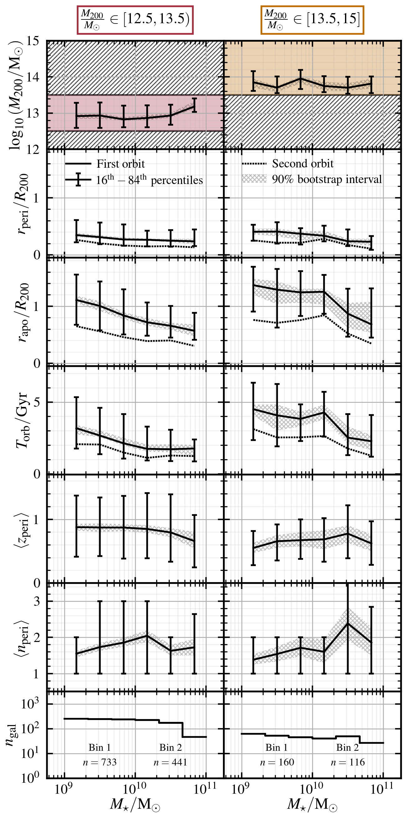
Figure 6: Properties of the selected infall orbits as a function of stellar mass. Each column pertains to different bins in host mass – left including satellites with host masses $M_{\rm 200}/{\rm M}_{\odot}\in[10^{12.5},10^{13.5})$ – red; and right including host masses $M_{\rm 200}/{\rm M}_{\odot}\in[10^{13.5},10^{15}]$ – orange. From top to bottom, each row illustrates: host halo mass, $M_{\rm 200}$); pericentric distance normalised by host virial radius, $r_{\rm peri}/R_{\rm 200}$; apocentric distance normalised by host virial radius, $r_{\rm apo}/R_{\rm 200}$; orbital time-scale, $T_{\rm orb}$; mean redshift of first pericenter, $\langle z_{\rm peri}\rangle$; mean number of pericenters survived (before halo lost or merged with central), $\langle n_{\rm peri}\rangle$; and a histogram of the number of satellites included in the sample as a function of stellar mass. Error-bars display the $16^{\rm th}-84^{\rm th}$ percentile range in each stellar mass bin, and cross-hatched regions denote the bootstrap-generated $90\%$ confidence interval on the medians (based on 500 re-samples). We only include bins where the statistics have been calculated with at least 20 galaxies.

In this subsection, we now move to statistically analyse our sample of satellite orbits. The orbital properties of the final sample as a function of stellar mass for each halo mass selection are shown in Fig. 6. We illustrate these orbital properties to demonstrate the potential biases introduced in each sample in the process of binning the orbits by pericentric stellar mass (as is done for the remainder of this section). The left-hand panel shows the results for the small group sample (red), and the right-hand columns provides the results for the larger group/cluster selection (orange). The number of satellites included for each stellar mass bin in the two halo mass samples is quoted in the bottom row of panels; with there being $\approx 3$ times as many orbits recorded for the group-mass sample compared to the larger group/cluster-mass sample.

We remark that our initial orbit selection included galaxies with stellar mass between $10^{8}{\rm M}_{\odot}$ and $10^{9}{\rm M}_{\odot}$ – however, we choose to focus on galaxies with $M_{\star}\geq 10^{9}{\rm M}_{\odot}$ such that there are ample gas and stellar particles in the galaxies and the influence of numerical effects is minimised.

The top row of panels in Fig. 6 illustrates that the two aforementioned halo mass selections do not introduce a significant bias in halo mass as a function of stellar mass. The group-mass sample shows a steady median halo mass at $\log(M_{\rm 200}/{\rm M_{\odot}})\$$\approx 13$, with a very slight upturn at $\log(M_{\star}/{\rm M_{\odot}})\$$\approx 11$. This slight upturn is likely due to the low probability of a halo with mass on the lower end of the $10^{12.5}-10^{13.5}{\rm M}_{\odot}$ sample hosting a massive satellite, with stellar mass in excess of $\approx 10^{10.5}{\rm M}_{\odot}$. The larger group/cluster sample (orange, right panel) also shows a steady median across stellar mass, slightly below $\log(M_{\rm 200}/{\rm M_{\odot}})\$$\approx 14$.

The second row of panels in Fig. 6 shows the first pericentric radius of satellite orbits in the two halo mass samples as a function of satellite stellar mass. For those satellites that survive to a second pericenter, we illustrate the mean second pericentric distance with dashed lines. In both halo mass samples, we observe that the measured pericentric radii decrease with increasing stellar mass – from $r_{\rm peri}/R_{200}\approx 0.5$ at $\log(M_{\star}/{\rm M_{\odot}})\$$\approx 9$ to $r_{\rm peri}/R_{200}\approx 0.25$ at $\log(M_{\star}/{\rm M_{\odot}})\$$\approx 11$. This bias is likely introduced by dynamical friction, as well as our requirement that the satellite survives pericenter and experiences at least one apocenter.

At smaller pericentric radii, the likelihood for satellite disruption is increased, particularly below $r_{\rm peri}/R_{200}\approx 0.3$ – roughly corresponding to the expected BMP radius of a central galaxy with $\log(M_{\star}/{\rm M_{\odot}})\$$>10-11$ (see bottom panel of Fig. 10). More massive satellites – with deeper gravitational wells and larger restoring forces – are less likely to be entirely disrupted by such passages, however this is not the case for low-mass satellites with $\log(M_{\star}/{\rm M_{\odot}})\$$\lesssim 9.5$ (see Figure 6, dark green curve in Bahé et al. 2019). This may also be a result of numerical issues given the small number of stellar and gas particles in these galaxies ($<1000$); and the fact that such systems are more likely to be lost in merger trees. We note that second pericentric distances are systematically lower than the original pericenter – decreased by a relatively steady fractional change in $r/R_{\rm 200}$ of $\approx 0.2$ for both halo mass bins, likely due to the effects of dynamical friction.

The third row of panels in Fig. 6 illustrates the first apocentric radius of satellite orbits. For those satellites that survive to a second apocenter, we also illustrate the mean second apocentric distance with the dashed lines. Similar to the pericentric distances discussed, there is a preference for low-mass galaxies to have larger apocentric distances – in this case extending to beyond the host virial radius for satellites with stellar mass below $10^{9}{\rm M}_{\odot}$. The difference between first and second apocentric distance is pronounced, with many second apocenters halving their halo-centric distance after completing a full orbit.

The larger orbital radius noted for low-mass satellites in rows 2 and 3 of Fig. 6 translates to longer orbital time-scales for these galaxies, which is explicitly demonstrated in the fourth row of panels. We measure orbital time-scales in our sample by doubling the time between pericenter and apocenter in the first orbit; and use the same procedure for the galaxies that survive a second orbit. We note that the precision of these measurements is limited by the cadence of the eagle snipshots – ranging between $50$ and $150$ Myr. For both halo mass samples, orbital time-scales decrease from $T_{\rm orb}\approx 4$ Gyr at $\log(M_{\star}/{\rm M_{\odot}})\$$\approx 9$ to $T_{\rm orb}\approx 2$ Gyr at $\log(M_{\star}/{\rm M_{\odot}})\$$\approx 11$. For galaxies that survive a second orbit, their orbital time-scales, on average, decrease by $\approx 1$ Gyr across stellar mass for the group-mass sample (left), and slightly more for the larger group/cluster sample (right) where the effects of dynamical friction are more significant. We note that it is important to consider this bias for longer orbital time-scales in the lower-mass satellites when interpreting the results in the remainder of this section.

The fifth row of panels in Fig. 6 shows the mean redshift of first pericenter as a function of stellar mass. For both samples we remark that there is no obvious bias (within the uncertainty) in accretion times of the satellites – with the mean redshift steady at $z\approx 0.7-0.8$ for the smaller group-mass sample and $z\approx 0.6$ for the larger group/cluster-mass sample. The lower pericentric redshift recorded for the cluster-mass sample is a reflection of the assembly age being anti-correlated with halo mass (De Lucia & Blaizot, 2007). We also note that the $16^{\rm th}-84^{\rm th}$ percentile spread in pericentric redshifts for the smaller group-mass sample is much higher than the cluster-mass sample, particularly towards higher redshift ($z\approx 1.5$).

The sixth row of panels in Fig. 6 shows the mean number of pericenters survived as a function of stellar mass for each halo mass sample. Our selection requires at least one pericenter and apocenter to be survived, and thus $1$ becomes the lowest possible $n_{\rm peri}$ value in our sample. In both samples, we unsurprisingly observe that the number of pericenters survived before disruption (as per the subfind trees) increases with stellar mass, from on average $\approx 1$ passage at $\log(M_{\star}/{\rm M_{\odot}})\$$\approx 9$ to $\approx 2$ passages at $\log(M_{\star}/{\rm M_{\odot}})\$$\approx 11$. For $\log(M_{\star}/{\rm M_{\odot}})\$$>10.5$, the upper percentile can extend to $3-4$ pericentric passages. This simply means that as we move towards larger time since pericentric passage (as in Figs. 7 and 8), our sample size, and thus statistical power, begins to decrease.

Finally, the bottom row of panels in Fig. 6 show the number of satellites included in the sample as a function of stellar mass (again using 3 bins per decade in stellar mass). In the smaller group-mass sample, the number of galaxies is largest in the stellar mass range $\log(M_{\star}/{\rm M_{\odot}})\$$\in[9,10]$ which contains $735$ satellites – however the peak is not dramatic, with the surrounding bins still containing $\approx 450$ satellites. In the larger group/cluster-mass sample, the number of galaxies is comparatively independent of stellar mass (with $\approx 120-160$ satellites included in the sample per decade in stellar mass).

With our selection in place, we move on to conduct a statistical analysis of satellite orbits by breaking our sample into $2$ bins of stellar mass – (i) intermediate-mass satellites, $\log(M_{\star}/{\rm M_{\odot}})\$$\in[9,10)$; and (ii) high-mass satellites, $\log(M_{\star}/{\rm M_{\odot}})\$$\in[10,11]$. We remind the reader that our initial orbit selection included galaxies with stellar mass between $10^{8}{\rm M}_{\odot}$ and $10^{9}{\rm M}_{\odot}$ – however, we choose to focus on galaxies with $M_{\star}\geq 10^{9}{\rm M}_{\odot}$ to reduce the influence of any numerical effects. In addition to stellar mass, we delineate between satellites orbiting hosts in small group haloes, $\log(M_{\rm 200}/{\rm M_{\odot}})\$$\in[12.5,13.5)$ – as per the second halo mass bin/red sample in §3; and larger group/cluster-mass haloes with $\log(M_{\rm 200}/{\rm M_{\odot}})\$$\in[13.5,15]$ – as per the third halo mass bin/orange sample in §3.

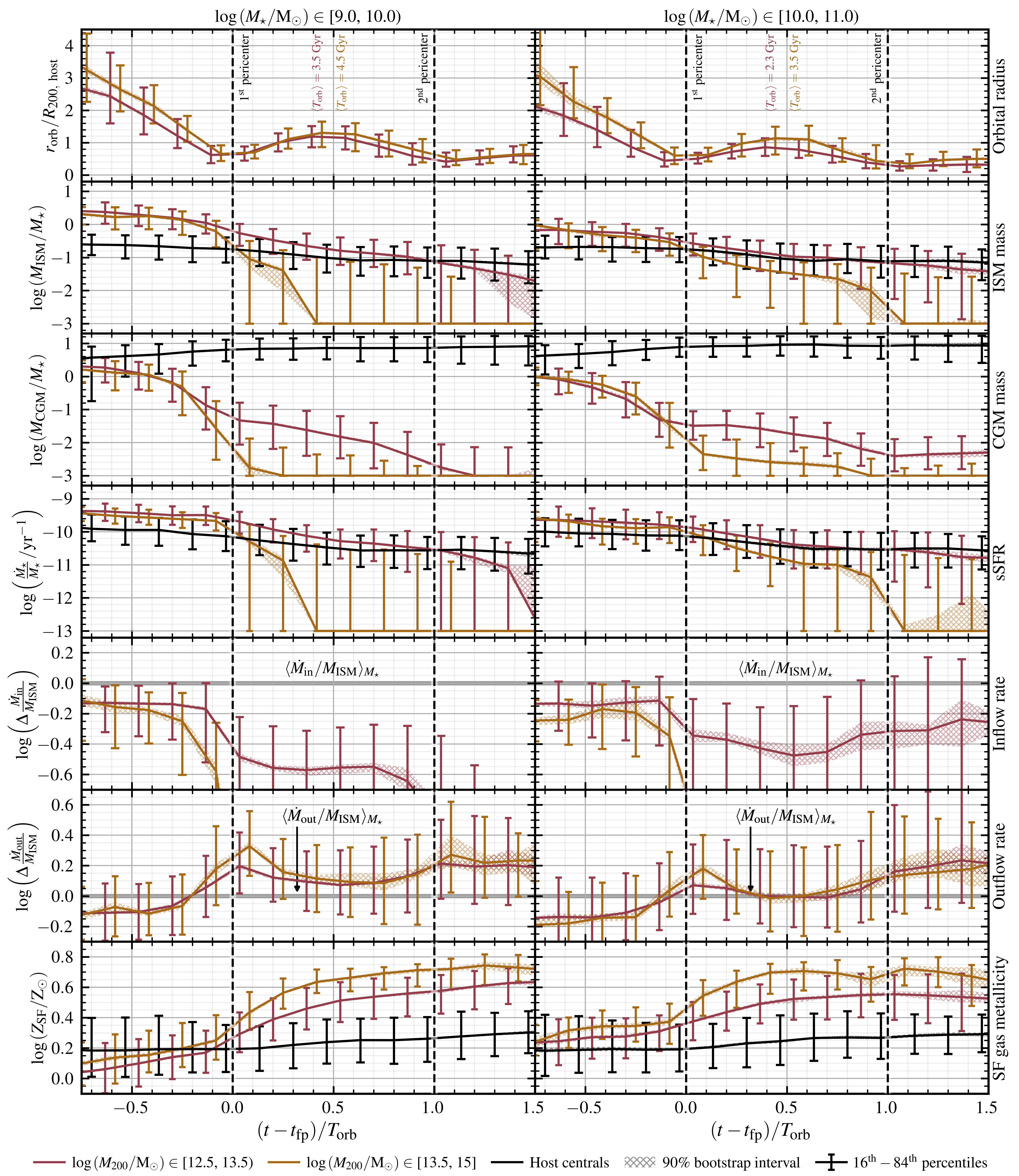
Figure 7: Various properties of satellite galaxies and host centrals as a function of orbital time, relative to first pericenter. In each panel, the results are shown for satellites with host masses ($M_{\rm 200}$) between $10^{12.5}{\rm M}_{\odot}-10^{13.5}$ ${\rm M}_{\odot}$ in red; $10^{13.5}{\rm M}_{\odot}-10^{15}{\rm M}_{\odot}$ in orange; and the median values for the central galaxies of these satellites (combined from both halo mass samples) in black. Each column shows the results for two bins in satellite stellar mass (at pericenter) – from left to right, $\log(M_{\star}/{\rm M_{\odot}})\$$\in[9,10)$; and $\log(M_{\star}/{\rm M_{\odot}})\$$\in[10,11)$. We stress that the selection of the host centrals for each sample is based on group mass alone, and that for the halo mass range considered $(M_{\rm 200}\geq 10^{12.5})$, such centrals will typically possess stellar mass of order $M_{\star}>10^{10.5}{\rm M}_{\odot}$. From top to bottom, each row illustrates the following median values along the orbit: orbital radius relative to host virial radius, $r_{\rm orb}/R_{200}$; ISM gas fraction, $M_{\rm ISM}/M_{\star}$; CGM mass (normalised by stellar mass), $M_{\rm CGM}/M_{\star}$; ${\rm sSFR}=\dot{M}_{\star}/M_{\star}$; excess ISM inflow rate, $\Delta\dot{M}_{\rm ISM,\ in}/M_{\rm ISM}$; excess ISM outflow rate, $\Delta\dot{M}_{\rm ISM,\ out}/M_{\rm ISM}$; and gas-phase metallicity of star-forming particles, $Z_{\rm SF}/{\rm Z}_{\odot}$. Error-bars display the $16^{\rm th}-84^{\rm th}$ percentile range in each stellar mass bin, and cross-hatched regions denote the bootstrap-generated $90\%$ confidence interval on the medians (based on 500 re-samples). We only include bins where the statistics have been calculated with at least 20 galaxies.

Moving forwards, splitting our selection into the aforementioned stellar and halo mass samples, we display a number of satellite properties as a function of orbital time in Fig. 7. In line with the work of Oman et al. (2021), we use the first pericentric passage as an objective time “zero point” – and also normalised by orbital time-scale to define the x-axis: $(t-t_{\rm fp})/T_{\rm orb}$. As outlined above, we calculate the orbital time-scale of satellites by doubling the interval between pericenter and apocenter for each orbit. Since we remove satellites that have been pre-processed, we note that in each satellite sample, the values presented in each row of panels at $(t-t_{\rm fp})/T_{\rm orb}\approx-0.75$ (left-most bin) approximately represent what would be expected of a field central galaxy with the same stellar mass (and are thus similar for both host mass samples pre-infall). We also remark that these pre-infall galaxies may indeed be ostensibly classified as central, with the requirement for selection in the satellite sample only enforced on satellite/central status at first pericenter. Based on the top row of panels, orbital distances pre-infall are, on average, outside $2-3R_{\rm 200}$ – where environmental effects are expected to be small (except when considering the hot gas reservoirs of lower mass satellites, Bahé et al. 2013). We note that the top row of panels also quotes the average orbital period for the first and second orbits of each sample.

We remind the reader that for inclusion in our sample, we require that a satellite reaches at least one apocenter in the merger trees – i.e. to $(t-t_{\rm fp})/T_{\rm orb}=0.5$. For $(t-t_{\rm fp})/T_{\rm orb}>0.5$, we include the results for satellites that survive longer than this minimum requirement – constituting a subset of the original sample. The mean number of pericenters survived as a function of stellar mass (for the original sample) is displayed in the second to bottom panel of Fig. 6. We also note that given a number satellites will share the same host halo, the results for host centrals will be biased towards more massive haloes in each sample – i.e., those that contain the most satellites (and likely, a relatively massive central galaxy). These values are simply provided for reference.

The top row of panels illustrates the orbital radius of satellites relative to $R_{200}$ of their host haloes. As noted in relation to Fig. 6, we see that pericentric and apocentric radii tend to decrease with stellar mass. Additionally, we see that apocentric radii decrease with the number of orbits completed for our selection – which we attribute to the effects of dynamical friction (De Lucia et al., 2012). Across stellar mass, the orbital radii between the two halo mass samples are statistically similar.

The second row of panels illustrates ISM mass (gas with $T\leq 5\times 10^{4}\ {\rm K}$ within $R_{\rm BMP}$) as a function of orbital time. ISM masses of zero are set to a floor value of $10^{6}{\rm M}_{\odot}$, slightly less than the mass of a single gas particle. Focusing on intermediate-mass satellites $\log(M_{\star}/{\rm M_{\odot}})\$$\in[9,10]$, we observe that the average satellite in this bin begins with a pre-infall ISM mass just below $\approx 10^{10}{\rm M}_{\odot}$. Full depletion of the ISM is normally complete by first apocenter in the large group/cluster sample, while, on average, it takes until second apocenter to fully deplete the satellites in the group-mass sample. Considering the high-mass satellites in the right-hand column, $\log(M_{\star}/{\rm M_{\odot}})\$$\in[10,11]$, we see more protracted depletion times; with satellites in the large group/cluster sample normally depleting all of their pre-infall gas (just above $\approx 10^{10}{\rm M}_{\odot}$) by second pericenter, and those in the group-mass host sample able to retain a gas mass of $>10^{9}{\rm M}_{\odot}$ even after second pericenter. Host central ISM mass, on average, shows a very slight decrease with orbital time for each sample, consistent with internally-driven gas consumption.

The third row of panels illustrates CGM mass (hot gas with $T>5\times 10^{4}\ {\rm K}$ associated with the satellite subhalo) as a function of orbital time. Focusing first on the intermediate-mass satellites, we observe that the onset of CGM stripping occurs quite early in all samples, at around $(t-t_{\rm fp})/T_{\rm orb}\approx-0.5$ or $r_{\rm orb}/R_{200}\approx 2$. Full CGM removal is expected for the large group/cluster sample at first pericenter, and for the smaller group sample at second pericenter. While all hot gas, on average, is expected to be stripped by second pericenter for intermediate-mass satellites the smaller group sample – we see this is not necessarily the case for the ISM reservoir, which is removed after some delay.

Considering the high-mass satellites, we note that the average CGM mass in this sample drops by a full $1.5$ dex ($10^{10}{\rm M}_{\odot}$ to $10^{8.5}{\rm M}_{\odot}$) from $(t-t_{\rm fp})/T_{\rm orb}\approx-1$ to first pericenter, however the hot gas is typically only fully depleted after a subsequent pericenter in the larger group/cluster sample, or reduced to $\approx 10^{8}{\rm M}_{\odot}$ in the small group sample. Between the stellar mass samples, it is clear that CGM hot gas stripping from satellites on infall precedes cool gas stripping. This agrees with the idea that the more tenuous, hot gaseous haloes surrounding infalling satellites are relatively easy to deplete with ram pressure given their increased spatial extent and reduced density (e.g Larson et al. 1980; Balogh et al. 2000; McCarthy et al. 2008; Bahé et al. 2013). Finally, we also note the growth of host central CGM mass to, on average, $10^{12}{\rm M}_{\odot}$ over the orbital times shown ($\approx 10$ Gyr) – likely due to a combination of IGM accretion and satellite stripping (Anglés-Alcázar et al., 2017; Mitchell et al., 2020b).

The fourth row of panels in Fig. 7 shows average specific star formation rates as a function of orbital time (i.e. the mass of new stars formed within $R_{\rm BMP}$ over the designated time interval), divided by stellar mass. For galaxies with a measured average star formation rate of zero, we set the sSFR to a floor value of $10^{-13}\ {\rm yr}^{-1}$. Prior to infall, each of the satellite samples show increased specific star formation rates ($>10^{-10}\ {\rm yr}^{-1}$) compared to the host central sample. This is a simple reflection of declining sSFR with stellar mass, which exists in the absence of environmental effects. We find that the departure of galaxies from their expected secular sSFR upon infall to a host is dependent on the mass of the satellite, and the mass of the host halo. In general, this departure very closely follows the depletion of ISM mass, as shown in the second row of columns (discussed above).

Interestingly, for satellites above $10^{9}{\rm M}_{\odot}$ in the small group sample, $\log(M_{\rm 200}/{\rm M_{\odot}})\$$\in[12.5,13.5)$, we measure the specific star formation rates to be very similar to the central galaxies even after a second pericenter. While the rate of star formation decline is steeper in these satellites than for the host centrals at this orbital time, the rate of change in star formation rate for these satellites is still quite slow – dropping $\approx 0.5$ dex in sSFR over a full orbital time-scale, compared to the host centrals where sSFR drops by $\approx 0.25$ dex over the same period. This agrees with empirical inferences of quenching occurring several Gyr after infall in low-mass groups (e.g. Wetzel et al. 2013; Wheeler et al. 2014).

The fifth and sixth row of panels in Fig. 7 illustrate the excess specific ISM inflow ($\Delta\dot{M}_{\rm in}/M_{\rm ISM}$) and outflow ($\Delta\dot{M}_{\rm out}/M_{\rm ISM}$) rates in satellites along their infall. Here, the term excess means that we have normalised the specific inflow and outflow rates by the flow rates experienced by central galaxies, controlled for their stellar mass and redshift – i.e. the flow rates “expected” in the absence of environmental effects. These expected flow rates were illustrated in Fig. 3 as a function of stellar mass.

Firstly, we note that inflow rates to the ISM of galaxies follow the behaviour of the CGM hot gas reservoir – i.e. the origin of this accreting gas. In both satellite samples, we observe a delay in the onset of inflow suppression subsequent to the onset of hot gas stripping. While hot gas begins to be stripped at $(t-t_{\rm fp})/T_{\rm orb}\approx-0.5$ or $r_{\rm orb}/R_{200}\approx 2-2.5$, this decrease in available gas to feed the galaxy only significantly influences inflow rates much closer to pericenter (well within $R_{\rm 200}$) in these samples.

We find that intermediate-mass satellites in large groups/clusters, on average, are completely cut-off from the accretion of new gas after first pericenter, while it requires 2 pericentric passages to achieve the same effect in a satellite of the same mass in a smaller group environment ($<10^{13.5}{\rm M}_{\odot}$). These findings match the typical time it takes to strip these satellite’s CGM gas reservoirs. In the high-mass satellite sample, we find that satellites on infall to large groups/clusters, on average, experience a reduction in accretion rates relative to ISM mass of 1 dex after first pericenter, and are completely cut-off from accretion after a second pericenter. Interestingly, it appears that higher-mass satellites in the smaller group sample, $\log(M_{\rm 200}/{\rm M_{\odot}})\$$\in[12.5,13.5)$, experience a relatively mild decrease in specific inflow rates (at maximum $\approx 0.3-0.4$ dex relative to the value expected for centrals – remaining steady at this value after first pericenter).

Concentrating on the excess outflow rates presented in the sixth row of panels in Fig. 7, we can see clear signatures of cool gas stripping along the orbit of satellites. Prior to infall, specific outflow rates in each sample are relatively uniform, sitting at a value slightly less than that expected in centrals. In each of these samples, we note a significant increase in outflow rates relative to centrals of $\approx 0.2-0.4$ dex approaching pericenter. We argue that this corresponds to the influence of ram pressure stripping, which is most prevalent at pericenters where orbital velocities peak ($P_{\rm ram}\propto v_{\rm orb}^{2}$). The peak in excess gas outflow is the greatest for intermediate mass satellites in large groups/clusters ($\log\Delta\dot{M}_{\rm in}/{M_{\rm ISM}}\approx 0.4$, $2-2.5$ times that experienced by central galaxies of the same mass) and is smallest in high-mass satellites in smaller group environments ($\log\Delta\dot{M}_{\rm in}/{M_{\rm ISM}}\approx 0.15$, enhanced $40\%$ relative to central galaxies of the same mass). We measure that the peak in excess outflow rates appears to occur just subsequent to first pericenter for both samples, however we remind the reader that the gas flux measured at a given time corresponds to the flow of gas that occurred over the 2 snipshots prior. Between pericenters, outflow rates reduce to slightly above that of centrals for intermediate-mass satellites, and to a level similar to centrals in high-mass satellites.

Finally, the bottom row of panels in Fig. 7 shows the gas-phase metallicity of star-forming gas in the ISM of satellites as a function of orbital time. The metallicity of galaxies is often used as a proxy for the age and/or star formation history of galaxy populations over time, with recent observational and theoretical literature indicating that satellites in higher-density environments exhibit a systematically increased (gas-phase) metallicity compared to the field (e.g. Cooper et al. 2008b; Davé et al. 2011; Pasquali et al. 2012; De Rossi et al. 2015; Genel 2016; Bahé et al. 2017a).

As fully explored in Schaye et al. (2015), we remark that the mass-metallicity relation in eagle does not match observations below $M_{\star}\approx 10^{10}{\rm M}_{\odot}$ at fiducial resolution. We note that here, however, our results focus on the relative change in ISM metallicity of satellites over their orbit – which we expect to be less sensitive to resolution effects.

Host central galaxies show a very gradual enhancement in metallicity over orbital time, increasing $\approx 0.1$ dex over the full time range shown and hovering near solar metallicity ($Z_{\rm ISM}\approx Z_{\odot}$) – consistent with internally driven enrichment from stellar evolution and feedback. For each sample of satellites, the increase in metallicity over the same time interval is significantly larger than their host centrals, ubiquitously $>0.4$ dex by second pericenter. Pre-infall metallicity differs between intermediate-mass satellites and high-mass satellites, beginning at $\log(Z_{\rm ISM}/{\rm Z}_{\odot})\approx 0$ and $\log(Z_{\rm ISM}/{\rm Z}_{\odot})\approx 0.2$ respectively. Both intermediate and high-mass satellites start to see significant increases in metallicity prior to first pericenter – $(t-t_{\rm fp})/T_{\rm orb}\approx-0.5$ – as the galaxy is starved of low-Z inflow.

In both intermediate and high-mass satellites, we find that ISM metallicities reach a maximum plateau value by first apocenter – $(t-t_{\rm fp})/T_{\rm orb}\approx 0.5$. In the small group sample, this plateau value sits at $\log(Z_{\rm ISM}/{\rm Z}_{\odot})\approx 0.6$, compared to the large group/cluster sample (host to more severe ISM stripping) at $\log(Z_{\rm ISM}/{\rm Z}_{\odot})\approx 0.8$. The absolute change in metallicity is larger for the intermediate mass satellites, which start with solar ISM metallicities compared to the high-mass sample, that show slightly super-solar pre-infall metallicities. This metallicity jump relative to field galaxies is higher than that typically quoted in observations, however, we note that the increase we observe is restricted to our sample of satellites that have definitively undergone an $R_{200}$ crossing and first pericentric passage.

Typically, gas that is radially further from the center of a galaxy exhibits lower metallicity due to the presence of freshly accreted low-$Z$ gas, and lower star formation-rate density (e.g. Bahé et al. 2017a; Collacchioni et al. 2020). Thus, the preferential removal of the less bound, low-$Z$ gas in satellites leads to an increase in the metallicity of the ISM, as the measurement becomes constricted to the more central regions. This is compounded by the lack of low metallicity gas inflow, which otherwise plays a key role in modulating the metallicity of the ISM (Collacchioni et al., 2020).

We note that while the relatively prolonged decrease in sSFR is clearly linked with decreasing ISM gas mass in satellites along their orbits, the rapid increase in gas-phase metallicity appears to be associated with the immediate removal of CGM gas at first-infall, and consequent lack of low-metallicity inflow. Our results also support the idea that the steep increase in gas-phase metallicity of satellites at first pericenter could be taken into account when inferring whether a satellite is still on first infall to a group, or has indeed experienced its first pericentric passage.

Holistically speaking, these findings support the conclusion that the more massive a satellite, the greater its propensity to retain a star-forming, cool gas reservoir (e.g. Hester 2006). Broadly, this prediction aligns with the observation that dwarf satellites within the Milky Way’s virial radius are quenched, while some satellites with $\log(M_{\star}/{\rm M_{\odot}})\$$>10$ in the Virgo cluster retain a significant amount of gas – even despite the latter environment having significantly higher density (and thus ram pressure stripping potential) compared to the Local Group (Cortese et al., 2021). This idea also agrees with the theoretical findings of Bahé & McCarthy (2015) and Oman et al. (2021), who find that the transition time-scales of satellites to being passive after infall are significantly shorter ($<500$ Myr) for satellites below $M_{\star}\approx 10^{10}{\rm M}_{\odot}$ compared to their higher mass counterparts using the GIMIC (Crain et al., 2009) and Hydrangea simulations respectively (Bahé et al., 2017b). The exact time-scale for quenching depends heavily on when the “zero” time is taken, which is commonly set to “infall”, or first pericenter (Cortese et al., 2021).

Wright et al. (2019) also show that the quenching time-scales of eagle satellites are significantly shortened ($<1$ Gyr) for galaxies with small stellar–halo mass ratios ($M_{\star}/{\rm M}_{\odot}<10^{-4}$; i.e. low-mass satellites in higher-mass haloes). Our findings suggest that some satellites can be fully quenched after just one pericentric passage – which we indeed find to be the expectation for satellites with stellar mass less than $10^{10}{\rm M}_{\odot}$ on infall to haloes above a mass of $10^{13.5}{\rm M}_{\odot}$; and even for satellites in less massive group haloes, between $10^{12.5}{\rm M}_{\odot}$ and $10^{13.5}{\rm M}_{\odot}$ when their stellar mass is less than $10^{9}{\rm M}_{\odot}$.

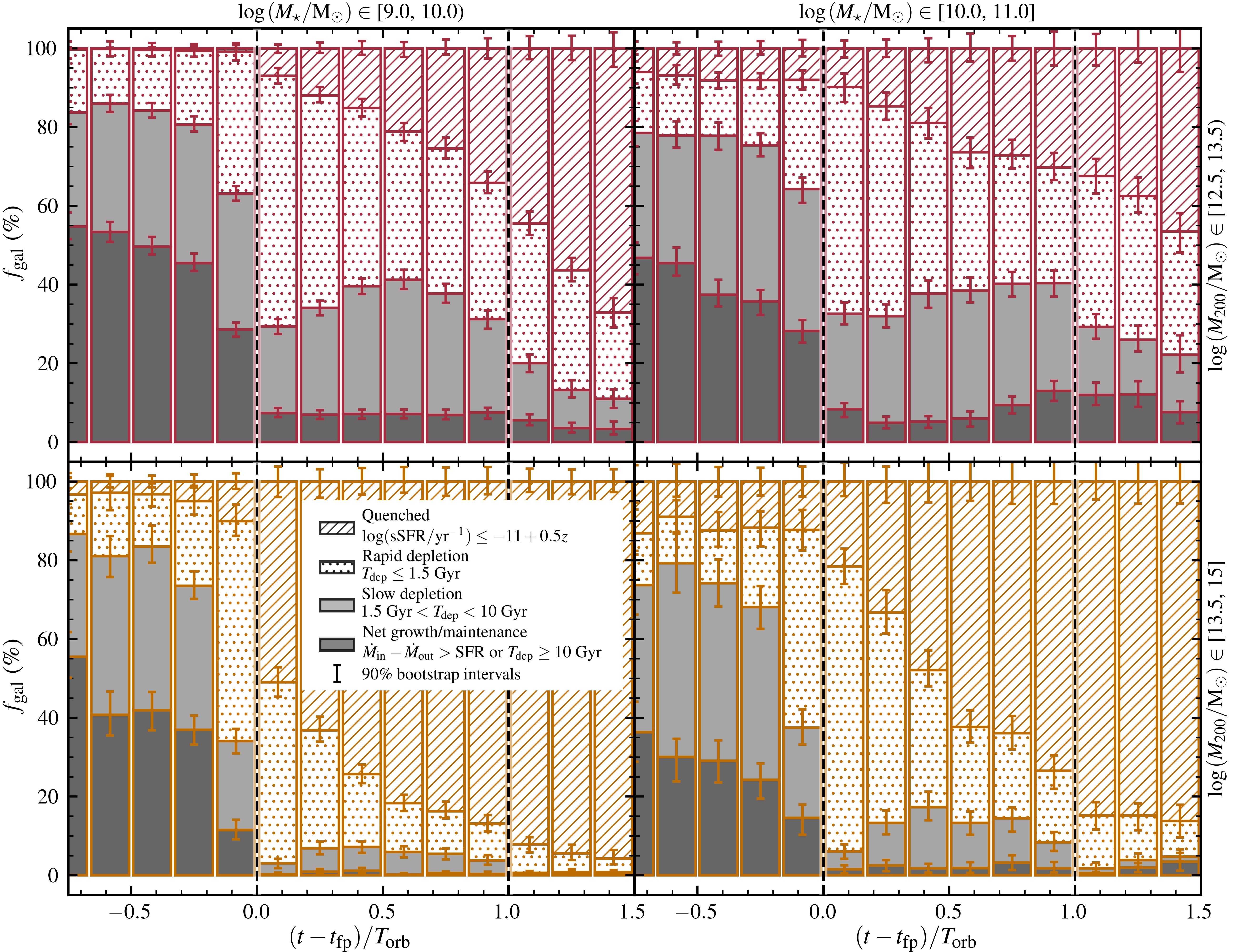
Figure 8: The breakdown of galaxies into gas flow classes (outlined in Table 2) as a function of orbital time relative to first pericentric passage. A galaxy can be classified as either (1) net growing/maintaining its ISM reservoir – dark grey shading; (2) slowly depleting its ISM reservoir – light grey shading; (3) rapidly depleting their ISM reservoir – dotted shading; and (4) quenched – forward-hatched shading. The delineating time-scale between “slow” and ”rapid” depletion is $1.5$ Gyr, based on the median quenching time-scale ($\tau_{\rm Q}$) value measured for eagle galaxies in Wright et al. (2019). Each column corresponds to a different bin in stellar mass, from left to right $\log(M_{\star}/{\rm M_{\odot}})\$$\in[9,10)$; and $\log(M_{\star}/{\rm M_{\odot}})\$$\in[10,11]$. Each row corresponds to a different halo mass bin, with the top panels illustrating the breakdown for satellites in group-mass haloes, $\log(M_{\rm 200}/{\rm M_{\odot}})\$$\in[12.5,13.5)$, red; and the bottom panels for satellites in larger group/cluster-mass haloes, $\log(M_{\rm 200}/{\rm M_{\odot}})\$$\in[13.5,15]$. Error-bars denote the bootstrap-generated $90\%$ confidence interval on the fractions (based on 500 re-samples).

Fig. 8 uses the gas flow classes outlined in Table 2 with average inflow, outflow and star formation rates shown in Fig. 7 to plot the changing evolutionary state of our different satellite samples along their orbits. We use the same satellite sample classifications (based on stellar and halo mass) as employed for Figs. 6 and 7. We also remind the reader that some pre-infall galaxies may indeed be technically classified as a central, with the requirement for selection in the satellite sample only enforced on satellite/central status at first pericenter.

Focusing on intermediate mass satellites, $\log(M_{\star}/{\rm M_{\odot}})\$$\in[9,10)$, we observe a more gradual transition to quiescence over their orbits in both halo mass samples. Pre-infall quenched fractions sit very close to zero – growing to $\approx 5\%$ at pericenter in the small group sample, and $\approx 50\%$ at pericenter in the large group/cluster sample. At second pericenter, the quenched fraction grows to $\approx 40\%$ in the small group sample, and $\approx 80\%$ in the large group/cluster sample. In the small-group sample (middle column, top panel), we note that the fraction of galaxies net growing their gas reservoir remains just above $5\%$ over the first orbit. In the same sample, the fraction of galaxies with rapid depletion time-scales is largest just after first pericenter ($\approx 60\%$) until apocenter, where the fraction of galaxies with longer predicted depletion time-scales ($>1.5$ Gyr) grows to $\approx 30\%$. Based on the results in Fig. 7, it appears that some galaxies in this sample (intermediate mass satellites in the small-group selection) are not completely cut-off from gas inflow after first pericenter, and at first apocenter, outflow rates reduce by a factor of a few relative to their value at pericenter. The combination of these factors means that such galaxies deplete their gas reservoirs relatively slowly – while inflow rates are not enough to fully replenish the ISM, the lack of stripping at apocenter slows the quenching process.

On approach to second pericenter, the fraction of quenched galaxies continues to increase and galaxies with slow depletion time-scales move to the fast-depletion group as outflow rates again increase. In the large group/cluster sample (middle column, bottom panel), we note that the likelihood of finding a slow-quenching galaxy at first apocenter is much lower ($<10\%$) than found for the small group sample. Referring to Fig. 7, we find that galaxies in this sample are fully cut off from fresh accretion after first pericenter, associated with more efficient stripping of the satellite’s CGM gas in the harsher group/cluster environment. We do not necessarily find there to be more severe specific ISM outflow rates compared to the less massive group sample, however the lack of replenishing gas means the quenching process is greatly accelerated for these galaxies between first and second pericenter.

The picture for high-mass satellites involves a slightly slower growth rate of the quenched population along their orbits. As per the ${M}_{\star}$–sSFR relation for central galaxies, the ${\rm sSFR}$ of these high-mass satellites has a pre-infall value slightly below the lower mass groups, and a correspondingly larger quenched fraction of $\approx 10\%$ compared to $<5\%$. At first pericenter, this value remains similar at $\approx 10\%$ in the small group sample, and grows to $\approx 15-20\%$ in the large group/cluster sample. At second pericenter, the quenched fraction grows to $\approx 35\%$ in the small group sample, and $\approx 80\%$ in the large group/cluster sample. While these second pericenter quenched fractions are similar to the intermediate-mass sample, the growth of the quenched fraction is slightly gentler given the higher pre-infall quenched fractions in this sample. We note a clear increase in the fraction of galaxies in the large group/cluster sample (right-most bottom panel) that are part of the slowly quenching group near first apocenter ($\approx 15\%$), compared to this fraction in the equivalent intermediate-mass sample ($<10\%$). We remark that this is likely due to the propensity of massive satellites to retain a CGM reservoir after first pericenter, and as such, still experience some level of ISM accretion (refer to Fig. 7). This is not the case for the intermediate-mass sample, which, on average, experiences more dramatic hot gas stripping (and thus starvation) after first pericenter.

The results presented in Figs. 7 and 8 highlight the importance of considering the interplay between gas inflows (or a lack thereof), together with hot and cold gas removal in satellites; and moreover, how these processes vary temporally along the orbit of these galaxies in driving their path towards quiescence in group environments. This path towards quiescence will typically begin with the removal of hot gas along first-infall, which becomes evident at $2-3$ virial radii and becomes more efficient with increasing host mass, decreasing satellite mass, and increasing orbital velocity (which is periodic, peaking at pericenters, and reducing at apocenters). Once significant hot gas removal has occurred, the galaxy will experience “starvation” – with no surrounding hot gas left to replenish the ISM reservoir. The depletion of this hot gas reservoir also subsequently allows direct cold gas (ISM) stripping, which also demonstrates periodic behaviour prior to complete depletion. In the absence of CGM gas, the efficiency of cold gas stripping is a strong function of host mass and satellite mass – with low-mass satellites in large group/cluster environments experiencing very efficient stripping in the absence of accretion, and higher-mass satellites experiencing less efficient stripping and a more gradual, starvation-like quenching scenario after their first pericenter.

Accounting for each of the above factors, our analysis leads to the following predictions for the quenching of satellites along their orbits in a group environment (with “quenching” defined by a threshold of $\log({\rm sSFR}/{\rm yr}^{-1})<-11+0.5z$). We predict that the average intermediate-mass satellite, $\log(M_{\star}/{\rm M_{\odot}})\$$\in[9,10]$, will be quenched subsequent to second pericenter in a small group environment; and will be quenched just after first pericenter in a large group/cluster environment. Secondly, we predict that $\approx 30\%$ of high mass satellites, $\log(M_{\star}/{\rm M_{\odot}})\$$\in[10,11)$, will be quenched after second pericenter in a small group environment; and that the average high-mass satellite will be quenched near first apocenter in a large group/cluster environment. The rate of growth of the quenched fraction is gradual in many cases, and as such, these orbital quenching predictions represent the averages within some spread.

5 Discussion and Summary

In this paper, we analyse the balance of gas flows in eagle satellite galaxies as a function of environment (§3) and orbital time (§4). To do so, we employ a robust methodology to define the ISM of eagle galaxies, and make use of the temporally finely-sampled eagle “snipshots” to fairly quantify and compare ISM inflow, outflow, and star formation rates.

In §3, we quantify how the gas inflow, outflow, and star formation rates compare in central and satellite galaxies as a function of environment in the context of the equilibrium model. For galaxies experiencing net ISM depletion, we can also use these flow rates to calculate an indicative ISM depletion time-scale. We find that:

• There is clear, environmentally-driven suppression in the gas accretion rates of satellite galaxies, becoming increasingly significant with increasing host halo mass (agreeing with the findings of van de Voort et al. 2017).

• When ISM gas mass is controlled for, the rate of specific gas outflow (accounting for both internal gas removal mechanisms and externally-driven stripping) increases with increasing halo mass in satellite galaxies.

• Central galaxies typically stay very close to equilibrium at redshifts $z<2$ – that is to say, inflow rates balance star formation and outflows. For those galaxies that do experience net gas depletion, their expected depletion time-scales are longer ($>1.5$ Gyr) than satellites.

• Satellites experience increasing net gas depletion with increasing halo mass, with many exhibiting expected depletion time-scales below $1$ Gyr.

• While the lack of gas inflow to satellites in large group/cluster mass haloes could completely explain their quenching, any sub-Gyr quenching time-scales require concurrent cold gas removal.

In §4, we make use the OrbWeaver code to quantify the orbits of satellites in the eagle simulations. We use this orbital catalogue to analyse the properties of satellites as a function of orbital time, defined by the time of first pericentric passage and normalised by orbital time-scale. With our orbital sample, we conclude that:

• Satellites begin their path to quiescence with the stripping of circum-galactic hot gas at $2-3$ virial radii from the host. This hot gas removal is most efficient in large group and cluster environments ($M_{200}>10^{13.5}M_{\odot}$), and takes longer for high-mass satellites ($M_{\star}>10^{10}M_{\odot}$).

• The removal of this hot gas is clearly correlated with (i) the onset of starvation – that is, a lack of gas inflow to the ISM; and (ii) the onset of cold gas stripping, where there is no longer a “buffer” between the ISM and surrounding intra-group/intra-cluster medium.

• In low-mass satellites, $\log(M_{\star}/{\rm M_{\odot}})\$$<10$, the suppression of gas inflow is typically permanent after hot gas stripping, which normally occurs at first pericenter. In contrast, some high-mass satellites, $\log(M_{\star}/{\rm M_{\odot}})\$$>10$, can maintain a small hot gas reservoir and experience continued ISM gas accretion after first pericenter.

• The efficiency of cold gas stripping is periodic, peaking at pericenters where the relative velocity between the satellite and intra-group/intra-cluster medium (and thus ram-pressure force, $P_{\rm ram}\propto v^{2}$) is maximised.

• The gas-phase metallicity of satellites in all mass samples increases dramatically (by $>0.5$ dex) around first pericenter. After this steep jump at first pericenter, gas metallicities increase relatively slowly.

• The prolonged reduction in SFR along the orbit of a satellite is closely-linked with ISM gas removal via outflows, while the relatively rapid removal of CGM gas at first-infall – and consequent lack of low-Z gas inflow to the ISM – appears to be linked with the rapid increase in gas-phase metallicity.

We also produce predictions for the expected quenching of satellites as a function of their orbital time, split by stellar and halo mass:

• The average intermediate-mass satellite, $\log(M_{\star}/{\rm M_{\odot}})\$$\in[9,10)$, will be quenched subsequent to a second pericenter in a small group-mass environment – $\log(M_{\rm 200}/{\rm M_{\odot}})\$$\in[12.5,13.5)$; and will be quenched just after first pericenter in a large group/cluster environment – $\log(M_{\rm 200}/{\rm M_{\odot}})\$$\in[13.5,15]$.

• Only $\approx 30\%$ of high-mass satellites, $\log(M_{\star}/{\rm M_{\odot}})\$$\in[10,11)$, will be fully quenched even after a second pericenter; while the average high-mass satellite will be quenched near first apocenter in a large group/cluster environment – $\log(M_{\rm 200}/{\rm M_{\odot}})\$$\in[13.5,15]$.

We remind the reader that our sample represents satellites that have largely experienced their first pericenter prior to $z=0.5$, and remark that the evolution of satellites on first-infall at $z\approx 0$ is likely to be slightly different. Given that $z\approx 0$ galaxies experience globally lower gas accretion rates and possess lower initial gas-fractions, it is likely that ISM depletion may occur over shorter time-scales in group environments

By quantifying the different gas flows and processes involved in the quenching of satellites along their orbits, our findings begin to break the degeneracy between different quenching mechanisms. Our results highlight the fact that both starvation – a lack of gas inflow; and cold gas stripping – direct gas removal from the ISM, occur simultaneously in satellites. The magnitude of the influence of each mechanism is strongly dependent on the way in which one defines each process – however we argue that each plays a comparable and necessary role in the eventual quenching of satellites.

Data Availability

Particle data from the set of the eagle runs used for our analysis are publicly available at http://dataweb.cosma.dur.ac.uk:8080/eagle-snapshots/. Galaxy gas flow rate catalogs are available upon request to the corresponding author.

Appendix A Defining the ISM and gas flows

Here we detail the methodology employed to define the ISM of eagle galaxies, together with the relevant gas inflow, outflow, and star formation rates presented in this paper. As mentioned in §2.3, for the purposes of this paper it was important for us to define the ISM of eagle galaxies in a manner as agnostic as possible to the galaxy’s central or satellite classification. We focus on gas flows to and from the “cool” gas reservoir of galaxies, reflecting what could be considered the gas linked to a neutral molecular (Lagos et al., 2015) or atomic (Bahé et al., 2016) phase.

A.1 Previous literature

Here we provide an overview of the different ISM definitions that have been utilised in previous studies to analyse gas flow rates in cosmological hydrodynamical simulations.

Focusing on gas inflow, van de Voort et al. (2017) define the ISM of both central and satellite galaxies in eagle by selecting star-forming particles within a $30$kpc aperture of a galaxy’s centre of potential. Gas particles with a non-zero SFR in eagle reflect a “cold” phase, meeting the metallicity-dependent density threshold and being within $0.5$ dex of the density-dependent temperature floor outlined in Schaye et al. (2015). In a similar manner, Correa et al. (2018b) define the ISM of eagle central galaxies by selecting particles within a radial distance of $0.15\times R_{\rm 200}$ of the host centre of potential, that are either (i) star forming, or (ii) part of the “atomic” ISM (with $n_{\rm H}>10^{-1}{\rm cm}^{-3}$ and $T<10^{5}{\rm K}$). Mitchell et al. (2020b) take a slightly different approach in defining the ISM of eagle central galaxies, including gas particles within $0.20\times R_{\rm 200}$ that are either (i) star forming, or (ii) meet an atomic-phase selection; selecting particles with $n_{\rm H}>10^{-2}{\rm cm}^{-3}$ that are within $0.5$ dex of the density-dependent temperature floor.

Each of these works quote accretion rates to galaxies as the mass flux of gas particles that were not part of the ISM of a galaxy at a snapshot $z_{\rm i}$, but do meet the ISM conditions at the subsequent snapshot $z_{\rm j}$. This mass flux is normalised by the time interval between snapshots $z_{\rm j}$ and $z_{\rm i}$, $\Delta t_{\rm ij}$. Instead focusing on outflows, Mitchell et al. (2020a) use the same ISM selection and simulation cadence as Mitchell et al. (2020b), imposing an additional average velocity requirement to ensure genuine outward radial movement of outflow particles. In this case, the outflow rate is computed as the mass flux of particles which were part of the ISM of a galaxy at a snapshot $z_{\rm i}$, do not meet the ISM conditions at the subsequent snapshot $z_{\rm j}$, and also meet the aforementioned average radial velocity requirement.

van de Voort et al. (2017) and Correa et al. (2018b) both implement a $\Delta t_{\rm ij}$ defined by the cadence of the $28$ eagle snapshots (including $9$ outputs between $z=0$ to $z=1$, and $8$ outputs between $z=1$ and $z=2$); while Mitchell et al. (2020a) and Mitchell et al. (2020b) instead use a $\Delta t_{\rm ij}$ defined by $200$ eagle “snipshot” outputs (including $65$ outputs between $z=0$ and $z=1$, and $36$ outputs between $z=1$ and $z=2$). The latter choice to use a finer time-cadence ensures that instantaneous outflow rates are converged, which can be artificially reduced by recycling material if a longer $\Delta t_{\rm ij}$ is used.

A.2 The “BaryMP” method

As outlined in §2.3 – to define the extent of a galaxy in a manner agnostic to central/satellite status, we employ the baryonic mass profile (BMP) fitting method described in Stevens et al. (2014). With this method, the cumulative radial baryonic mass profile of “cool” gas (particles with either $T<5\times 10^{4}$ K or non-zero SFR) and stellar particles is analysed for a given (sub)halo to identify the best-fit transition point in the profile where $\rho_{\rm bar}(r)\propto r^{-2}$. This is a good approximation for an isothermal diffuse hot gas halo, as well as for a DM halo in virial equilibrium at the scale radius (Navarro et al., 1996). Following the BMP fitting process, the ISM of a galaxy is then defined by all cool gas particles ($T<5\times 10^{4}$ K or non-zero SFR) internal to this radius ($R_{\rm BMP}$). Fig. 9 demonstrates the BMP fitting process for a $\log(M_{\star}/{\rm M_{\odot}})\$$\approx 11$ eagle galaxy at $z=0$.

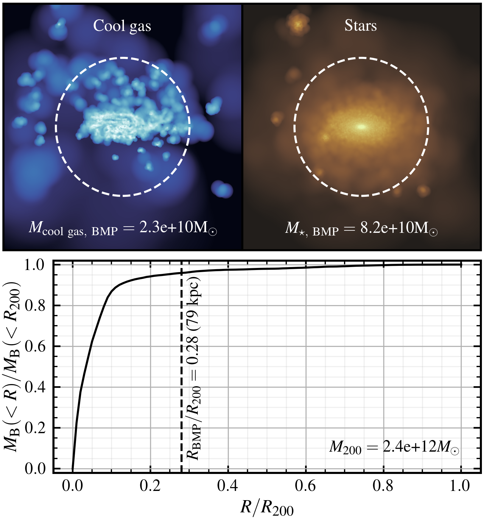
Figure 9: The “BaryMP” (BMP) fitting process for a $z=0$ $\log(M_{\star}/{\rm M_{\odot}})\$$\approx 11$ galaxy (based on Stevens et al. 2014). The cumulative mass profile of cool gas (${\rm SFR}>0$ or $T<5\times 10^{4}$ K; top left panel) and stars (top right panel) is fit to find the point at which the profile becomes effectively isothermal. In this case the BMP radius is found to be $79$ pkpc, as indicated by the dashed lines in each panel.

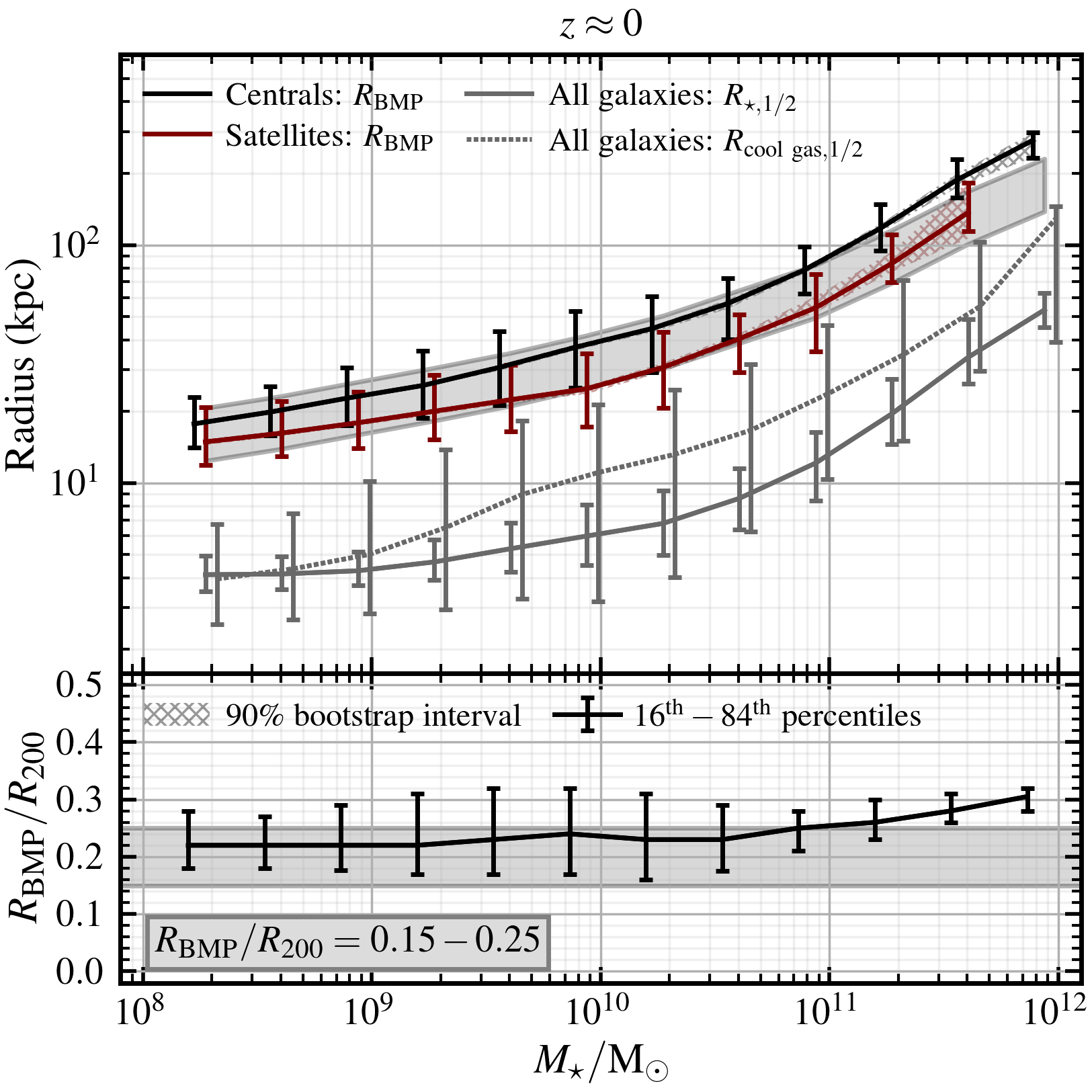
Figure 10: Top panel: the median BMP radius, $R_{\rm BMP}$ as a function of stellar mass internal to this radius, $M_{\star,\rm\ BMP}$, for $z\approx 0$ eagle central (black) and satellite (red) galaxies. For reference, we also illustrate the stellar half-mass radius ($R_{\star,1/2}$, solid line) and cool gas half-mass radius ($R_{\rm cool\ gas,1/2}$, dotted line) for all galaxies in grey. Bottom panel: the median ratio of $R_{\rm BMP}$ to the host $R_{\rm 200}$ virial radius for $z\approx 0$ central galaxies only. At fixed stellar mass, centrals exhibit systematically larger $R_{\rm BMP}$ values compared to satellites, by $\approx 0.1$ dex on average.

Fig. 10 demonstrates the results of the BMP fitting process for $z\approx 0$ eagle galaxies, split by central/satellite status. The top panel illustrates the median BMP radius, $R_{\rm BMP}$, as a function of stellar mass internal to this radius, $M_{\star,\rm\ BMP}$. Focusing on central galaxies (black), $R_{\rm BMP}$ increases with mass from a median of $25$ kpc at $\log(M_{\star}/{\rm M_{\odot}})\$$\approx 9$ to $300$ kpc at $\log(M_{\star}/{\rm M_{\odot}})\$$\approx 12$. The spread, as indicated by the grey shaded region, is largest for less massive systems, $\log(M_{\star}/{\rm M_{\odot}})\$$<10.5$. In this regime, the $16^{\rm th}-84^{\rm th}$ percentile range remains at $\approx 0.2$ dex, while for more massive systems, $\log(M_{\star}/{\rm M_{\odot}})\$$>11$, this spread reduces to $\approx 0.1$ dex.

In the top panel of Fig. 10 we also illustrate the stellar half-mass radius ($R_{\star,1/2}$) and cool gas half-mass radius ($R_{\rm cool\ gas,1/2}$) for all galaxies in grey. We note that these half-mass radii are calculated based on the particles within an aperture of $R_{\rm BMP}$. The reader may notice that while the half-mass radii follow the same functional form as the BMP radii with stellar mass, the $R_{\rm BMP}$ values (corresponding closely to $0.15-0.25\times R_{200}$) are significantly larger than $R_{\star,1/2}$. This highlights the fact that the BMP radius acts as an upper radial limit for the inclusion of particles in the stellar and ISM selection. In the case of cool gas, the temperature cut ($T<5\times 10^{4}$ K) preferentially selects gas that is well within the $R_{\rm BMP}$ radius. Above $M_{\star}\approx 10^{10}{\rm M}_{\odot}$, the half-mass radius of cool gas is a factor of $\approx 2$ larger than the stellar half-mass radius, meaning that on average, our ISM selection corresponds to a gas distribution that is slightly extended relative to the stellar component.

The bottom panel of Fig. 10 shows the ratio of $R_{\rm BMP}$ to the host halo virial radius, $R_{\rm 200}$, for central galaxies. The median $R_{\rm BMP}/R_{\rm 200}$ fraction ranges between $0.2-0.3$ for the majority of the mass range, exceeding 0.3 for the most massive galaxies, $\log(M_{\star}/{\rm M_{\odot}})\$$>11.5$. These $R_{\rm BMP}/R_{\rm 200}$ values slightly exceed the radial cuts used for central galaxies in Correa et al. (2018b) and Mitchell et al. (2020b).

Comparing centrals and satellite galaxies in the top panel of Fig. 10, we note that median $R_{\rm BMP}$ values for central galaxies systematically exceed satellite $R_{\rm BMP}$ measurements by $\approx 0.1-0.2$ dex ($25-50\%$) over the full mass range considered. Satellite galaxies with $\log(M_{\star}/{\rm M_{\odot}})\$$\approx 10-11$ exhibit higher variance in baryonic radii compared to centrals, with a $16^{\rm th}-84^{\rm th}$ percentile range of $\approx 0.3$ dex. The more concentrated baryonic mass profiles associated with satellites are likely a reflection of their reduced gas content compared to centrals; in which case $R_{\rm BMP}$ is primarily set by the stellar component.

References

- Anglés-Alcázar et al. (2017) Anglés-Alcázar D., Faucher-Giguère C.-A., Kereš D., Hopkins P. F., Quataert E., Murray N., 2017, MNRAS, 470, 4698
- Bahé & McCarthy (2015) Bahé Y. M., McCarthy I. G., 2015, MNRAS, 447, 969
- Bahé et al. (2013) Bahé Y. M., McCarthy I. G., Balogh M. L., Font A. S., 2013, MNRAS, 430, 3017
- Bahé et al. (2016) Bahé Y. M., et al., 2016, MNRAS, 456, 1115
- Bahé et al. (2017a) Bahé Y. M., Schaye J., Crain R. A., McCarthy I. G., Bower R. G., Theuns T., McGee S. L., Trayford J. W., 2017a, MNRAS, 464, 508
- Bahé et al. (2017b) Bahé Y. M., et al., 2017b, MNRAS, 470, 4186
- Bahé et al. (2019) Bahé Y. M., et al., 2019, MNRAS, 485, 2287
- Baldry et al. (2004) Baldry I. K., Glazebrook K., Brinkmann J., Ivezić Ž., Lupton R. H., Nichol R. C., Szalay A. S., 2004, ApJ, 600, 681
- Baldry et al. (2006) Baldry I. K., Balogh M. L., Bower R. G., Glazebrook K., Nichol R. C., Bamford S. P., Budavari T., 2006, MNRAS, 373, 469
- Balogh & Morris (2000) Balogh M. L., Morris S. L., 2000, MNRAS, 318, 703
- Balogh et al. (1999) Balogh M. L., Morris S. L., Yee H. K. C., Carlberg R. G., Ellingson E., 1999, ApJ, 527, 54
- Balogh et al. (2000) Balogh M. L., Navarro J. F., Morris S. L., 2000, ApJ, 540, 113
- Balogh et al. (2004) Balogh M. L., Baldry I. K., Nichol R., Miller C., Bower R., Glazebrook K., 2004, ApJ, 615, L101
- Baugh et al. (2019) Baugh C. M., et al., 2019, MNRAS, 483, 4922
- Bekki (2014) Bekki K., 2014, MNRAS, 438, 444
- Blanton et al. (2003) Blanton M. R., et al., 2003, ApJ, 594, 186
- Boselli & Gavazzi (2006) Boselli A., Gavazzi G., 2006, PASP, 118, 517
- Boselli et al. (2016) Boselli A., et al., 2016, A&A, 596, A11
- Bouché et al. (2010) Bouché N., et al., 2010, ApJ, 718, 1001
- Brinchmann et al. (2004) Brinchmann J., Charlot S., White S. D. M., Tremonti C., Kauffmann G., Heckman T., Brinkmann J., 2004, MNRAS, 351, 1151
- Brown et al. (2017) Brown T., et al., 2017, MNRAS, 466, 1275
- Calette et al. (2021) Calette A. R., Avila-Reese V., Rodríguez-Puebla A., Lagos C. d. P., Catinella B., 2021, MNRAS, 505, 304
- Cañas et al. (2019) Cañas R., Elahi P. J., Welker C., del P Lagos C., Power C., Dubois Y., Pichon C., 2019, MNRAS, 482, 2039
- Catinella et al. (2018) Catinella B., et al., 2018, MNRAS, 476, 875
- Chabrier (2003) Chabrier G., 2003, PASP, 115, 763
- Cole et al. (2000) Cole S., Lacey C. G., Baugh C. M., Frenk C. S., 2000, MNRAS, 319, 168
- Collacchioni et al. (2020) Collacchioni F., Lagos C. D. P., Mitchell P. D., Schaye J., Wisnioski E., Cora S. A., Correa C. A., 2020, MNRAS, 495, 2827
- Cooper et al. (2008a) Cooper M. C., et al., 2008a, MNRAS, 383, 1058
- Cooper et al. (2008b) Cooper M. C., Tremonti C. A., Newman J. A., Zabludoff A. I., 2008b, MNRAS, 390, 245
- Cora et al. (2018) Cora S. A., et al., 2018, MNRAS, 479, 2
- Correa et al. (2018a) Correa C. A., Schaye J., Wyithe J. S. B., Duffy A. R., Theuns T., Crain R. A., Bower R. G., 2018a, MNRAS, 473, 538
- Correa et al. (2018b) Correa C. A., Schaye J., van de Voort F., Duffy A. R., Wyithe J. S. B., 2018b, MNRAS, 478, 255
- Correa et al. (2019) Correa C. A., Schaye J., Trayford J. W., 2019, MNRAS, 484, 4401
- Cortese et al. (2021) Cortese L., Catinella B., Smith R., 2021, Publ. Astron. Soc. Australia, 38, e035
- Crain et al. (2009) Crain R. A., et al., 2009, MNRAS, 399, 1773
- Crain et al. (2015) Crain R. A., et al., 2015, MNRAS, 450, 1937
- Crain et al. (2017) Crain R. A., et al., 2017, MNRAS, 464, 4204
- Dalla Vecchia & Schaye (2012) Dalla Vecchia C., Schaye J., 2012, MNRAS, 426, 140
- Davé et al. (2011) Davé R., Finlator K., Oppenheimer B. D., 2011, MNRAS, 416, 1354
- Davé et al. (2020) Davé R., Crain R. A., Stevens A. R. H., Narayanan D., Saintonge A., Catinella B., Cortese L., 2020, MNRAS, 497, 146
- Davies et al. (2016) Davies L. J. M., et al., 2016, MNRAS, 461, 458
- Davies et al. (2019a) Davies L. J. M., et al., 2019a, MNRAS, 483, 1881
- Davies et al. (2019b) Davies L. J. M., et al., 2019b, MNRAS, 483, 5444
- Davis et al. (2014) Davis T. A., et al., 2014, MNRAS, 444, 3427
- De Lucia & Blaizot (2007) De Lucia G., Blaizot J., 2007, MNRAS, 375, 2
- De Lucia et al. (2012) De Lucia G., Weinmann S., Poggianti B. M., Aragón-Salamanca A., Zaritsky D., 2012, MNRAS, 423, 1277
- De Rossi et al. (2015) De Rossi M. E., Theuns T., Font A. S., McCarthy I. G., 2015, MNRAS, 452, 486
- Dekel & Mandelker (2014) Dekel A., Mandelker N., 2014, MNRAS, 444, 2071
- Dolag et al. (2009) Dolag K., Borgani S., Murante G., Springel V., 2009, MNRAS, 399, 497
- Donnari et al. (2019) Donnari M., et al., 2019, MNRAS, 485, 4817
- Donnari et al. (2021) Donnari M., Pillepich A., Nelson D., Marinacci F., Vogelsberger M., Hernquist L., 2021, MNRAS, 506, 4760
- Faucher-Giguère et al. (2011) Faucher-Giguère C.-A., Kereš D., Ma C.-P., 2011, MNRAS, 417, 2982
- Fossati et al. (2018) Fossati M., et al., 2018, A&A, 614, A57
- Furlong et al. (2015) Furlong M., et al., 2015, MNRAS, 450, 4486
- Genel (2016) Genel S., 2016, ApJ, 822, 107
- Giovanelli & Haynes (1985) Giovanelli R., Haynes M. P., 1985, ApJ, 292, 404
- Gómez et al. (2003) Gómez P. L., et al., 2003, ApJ, 584, 210
- Grootes et al. (2017) Grootes M. W., et al., 2017, AJ, 153, 111
- Gunn & Gott (1972) Gunn J. E., Gott J. Richard I., 1972, ApJ, 176, 1
- Haardt & Madau (2001) Haardt F., Madau P., 2001, in Neumann D. M., Tran J. T. V., eds, Clusters of Galaxies and the High Redshift Universe Observed in X-rays. p. 64
- Haines et al. (2015) Haines C. P., et al., 2015, ApJ, 806, 101
- Harris et al. (2020) Harris C. R., et al., 2020, Nature, 585, 357
- Hester (2006) Hester J. A., 2006, ApJ, 647, 910
- Hirschmann et al. (2014) Hirschmann M., De Lucia G., Wilman D., Weinmann S., Iovino A., Cucciati O., Zibetti S., Villalobos Á., 2014, MNRAS, 444, 2938
- Hunter (2007) Hunter J. D., 2007, Computing in Science and Engineering, 9, 90
- Jáchym et al. (2019) Jáchym P., et al., 2019, ApJ, 883, 145
- Jenkins (2013) Jenkins A., 2013, MNRAS, 434, 2094
- Katsianis et al. (2021) Katsianis A., et al., 2021, MNRAS, 500, 2036
- Kauffmann et al. (2003) Kauffmann G., et al., 2003, MNRAS, 341, 33
- Kauffmann et al. (2004) Kauffmann G., White S. D. M., Heckman T. M., Ménard B., Brinchmann J., Charlot S., Tremonti C., Brinkmann J., 2004, MNRAS, 353, 713
- Kennicutt (1983) Kennicutt R. C., 1983, The Astrophysical Journal, 272, 54
- Kereš et al. (2005) Kereš D., Katz N., Weinberg D. H., Davé R., 2005, MNRAS, 363, 2
- Knobel et al. (2013) Knobel C., et al., 2013, ApJ, 769, 24
- Krumholz & Matzner (2009) Krumholz M. R., Matzner C. D., 2009, ApJ, 703, 1352
- Lagos et al. (2015) Lagos C. d. P., et al., 2015, MNRAS, 452, 3815
- Lagos et al. (2018) Lagos C. d. P., Tobar R. J., Robotham A. S. G., Obreschkow D., Mitchell P. D., Power C., Elahi P. J., 2018, MNRAS, 481, 3573
- Larson (1972) Larson R. B., 1972, Nature, 236, 21
- Larson et al. (1980) Larson R. B., Tinsley B. M., Caldwell C. N., 1980, ApJ, 237, 692
- Lilly et al. (2013) Lilly S. J., Carollo C. M., Pipino A., Renzini A., Peng Y., 2013, ApJ, 772, 119
- Lotz et al. (2019) Lotz M., Remus R.-S., Dolag K., Biviano A., Burkert A., 2019, MNRAS, 488, 5370
- Marasco et al. (2016) Marasco A., Crain R. A., Schaye J., Bahé Y. M., van der Hulst T., Theuns T., Bower R. G., 2016, MNRAS, 461, 2630
- Martig et al. (2009) Martig M., Bournaud F., Teyssier R., Dekel A., 2009, ApJ, 707, 250
- McCarthy et al. (2008) McCarthy I. G., Frenk C. S., Font A. S., Lacey C. G., Bower R. G., Mitchell N. L., Balogh M. L., Theuns T., 2008, MNRAS, 383, 593
- Mitchell et al. (2020a) Mitchell P. D., Schaye J., Bower R. G., Crain R. A., 2020a, MNRAS, 494, 3971
- Mitchell et al. (2020b) Mitchell P. D., Schaye J., Bower R. G., 2020b, MNRAS, 497, 4495
- Moretti et al. (2020) Moretti A., et al., 2020, ApJ, 889, 9
- Navarro et al. (1996) Navarro J. F., Frenk C. S., White S. D. M., 1996, ApJ, 462, 563
- Nelson et al. (2015) Nelson D., Genel S., Vogelsberger M., Springel V., Sijacki D., Torrey P., Hernquist L., 2015, MNRAS, 448, 59
- Oman & Hudson (2016) Oman K. A., Hudson M. J., 2016, MNRAS, 463, 3083
- Oman et al. (2021) Oman K. A., Bahé Y. M., Healy J., Hess K. M., Hudson M. J., Verheijen M. A. W., 2021, MNRAS, 501, 5073
- Oort (1970) Oort J. H., 1970, A&A, 7, 381
- Pasquali et al. (2012) Pasquali A., Gallazzi A., van den Bosch F. C., 2012, MNRAS, 425, 273
- Peng & Renzini (2020) Peng Y.-j., Renzini A., 2020, MNRAS, 491, L51
- Peng et al. (2010) Peng Y.-j., et al., 2010, ApJ, 721, 193
- Peng et al. (2012) Peng Y.-j., Lilly S. J., Renzini A., Carollo M., 2012, ApJ, 757, 4
- Planck Collaboration et al. (2014) Planck Collaboration et al., 2014, A&A, 571, A16
- Poole et al. (2017) Poole G. B., Mutch S. J., Croton D. J., Wyithe S., 2017, MNRAS, 472, 3659
- Poulton (2019) Poulton R., 2019, OrbWeaver: Galaxy/(sub)halo orbital processing tool (ascl:1911.019)
- Poulton et al. (2020) Poulton R. J., Power C., Robotham A. S., Elahi P. J., 2020, MNRAS, 491, 3820
- Robotham et al. (2014) Robotham A. S. G., et al., 2014, MNRAS, 444, 3986
- Saintonge et al. (2017) Saintonge A., et al., 2017, ApJS, 233, 22
- Schaller et al. (2015) Schaller M., Dalla Vecchia C., Schaye J., Bower R. G., Theuns T., Crain R. A., Furlong M., McCarthy I. G., 2015, MNRAS, 454, 2277
- Schaye et al. (2007) Schaye J., Carswell R. F., Kim T.-S., 2007, MNRAS, 379, 1169
- Schaye et al. (2015) Schaye J., et al., 2015, MNRAS, 446, 521
- Somerville et al. (2008) Somerville R. S., Hopkins P. F., Cox T. J., Robertson B. E., Hernquist L., 2008, MNRAS, 391, 481
- Springel (2005) Springel V., 2005, MNRAS, 364, 1105
- Springel et al. (2001) Springel V., Yoshida N., White S. D. M., 2001, New Astron., 6, 79
- Springel et al. (2005) Springel V., Di Matteo T., Hernquist L., 2005, ApJ, 620, L79
- Steinhauser et al. (2016) Steinhauser D., Schindler S., Springel V., 2016, A&A, 591, A51
- Stevens & Brown (2017) Stevens A. R. H., Brown T., 2017, MNRAS, 471, 447
- Stevens et al. (2014) Stevens A. R., Martig M., Croton D. J., Feng Y., 2014, MNRAS, 445, 239
- Stevens et al. (2019) Stevens A. R. H., et al., 2019, MNRAS, 483, 5334
- Strateva et al. (2001) Strateva I., et al., 2001, AJ, 122, 1861
- Taranu et al. (2014) Taranu D. S., Hudson M. J., Balogh M. L., Smith R. J., Power C., Oman K. A., Krane B., 2014, MNRAS, 440, 1934
- Taylor et al. (2015) Taylor E. N., et al., 2015, MNRAS, 446, 2144
- Thorne et al. (2021) Thorne J. E., et al., 2021, MNRAS, 505, 540
- Tinsley & Danly (1980) Tinsley B. M., Danly L., 1980, ApJ, 242, 435
- Tonnesen & Bryan (2009) Tonnesen S., Bryan G. L., 2009, ApJ, 694, 789
- Trayford et al. (2016) Trayford J. W., Theuns T., Bower R. G., Crain R. A., Lagos C. d. P., Schaller M., Schaye J., 2016, MNRAS, 460, 3925
- Treyer et al. (2018) Treyer M., et al., 2018, MNRAS, 477, 2684
- Troncoso-Iribarren et al. (2020) Troncoso-Iribarren P., Padilla N., Santander C., Lagos C. D. P., García-Lambas D., Rodríguez S., Contreras S., 2020, MNRAS, 497, 4145
- Virtanen et al. (2020) Virtanen P., et al., 2020, Nature Methods, 17, 261
- Weinmann et al. (2009) Weinmann S. M., Kauffmann G., van den Bosch F. C., Pasquali A., McIntosh D. H., Mo H., Yang X., Guo Y., 2009, MNRAS, 394, 1213
- Wetzel et al. (2012) Wetzel A. R., Tinker J. L., Conroy C., 2012, MNRAS, 424, 232
- Wetzel et al. (2013) Wetzel A. R., Tinker J. L., Conroy C., van den Bosch F. C., 2013, MNRAS, 432, 336
- Wheeler et al. (2014) Wheeler C., Phillips J. I., Cooper M. C., Boylan-Kolchin M., Bullock J. S., 2014, MNRAS, 442, 1396
- White & Frenk (1991) White S. D. M., Frenk C. S., 1991, ApJ, 379, 52
- Wiersma et al. (2009) Wiersma R. P. C., Schaye J., Theuns T., Dalla Vecchia C., Tornatore L., 2009, MNRAS, 399, 574
- Wright et al. (2019) Wright R. J., Lagos C. d. P., Davies L. J. M., Power C., Trayford J. W., Wong O. I., 2019, MNRAS, 487, 3740
- Wright et al. (2020) Wright R. J., Lagos C. d. P., Power C., Mitchell P. D., 2020, MNRAS, 498, 1668
- Wyder et al. (2007) Wyder T. K., et al., 2007, ApJS, 173, 293
- Xie et al. (2020) Xie L., De Lucia G., Hirschmann M., Fontanot F., 2020, MNRAS, 498, 4327
- Zoldan et al. (2017) Zoldan A., De Lucia G., Xie L., Fontanot F., Hirschmann M., 2017, MNRAS, 465, 2236
- van Rossum & Drake Jr (1995) van Rossum G., Drake Jr F. L., 1995, Python reference manual. Centrum voor Wiskunde en Informatica Amsterdam
- van de Voort et al. (2011) van de Voort F., Schaye J., Booth C. M., Haas M. R., Dalla Vecchia C., 2011, MNRAS, 414, 2458
- van de Voort et al. (2017) van de Voort F., Bahé Y. M., Bower R. G., Correa C. A., Crain R. A., Schaye J., Theuns T., 2017, MNRAS, 466, 3460
- van den Bosch et al. (2008) van den Bosch F. C., Aquino D., Yang X., Mo H. J., Pasquali A., McIntosh D. H., Weinmann S. M., Kang X., 2008, MNRAS, 387, 79