Probing WIMPs in space-based gravitational wave experiments

Abstract

Although searches for dark matter have lasted for decades, no convincing signal has been found without ambiguity in underground detections, cosmic ray observations, and collider experiments. We show by example that gravitational wave (GW) observations can be a supplement to dark matter detections if the production of dark matter follows a strong first-order cosmological phase transition. We explore this possibility in a complex singlet extension of the standard model with CP symmetry. We demonstrate three benchmarks in which the GW signals from the first-order phase transition are loud enough for future space-based GW observations, for example, BBO, U-DECIGO, LISA, Taiji, and TianQin. While satisfying the constraints from the XENON1T experiment and the Fermi-LAT gamma-ray observations, the dark matter candidate with its mass around $\sim 1$ TeV in these scenarios has a correct relic abundance obtained by the Planck observations of the cosmic microwave background radiation.

Introduction– Although mounting evidence collected from cosmological Planck2016 and astrophysical Rubin1970APJ observations suggests that the dominant component of matter in our universe is the dark matter (DM), its nature still remains a myth even after about eighty years since its first discovery. Among various DM particle scenarios, one of the most promising DM candidates is the weakly interacting massive particles (WIMPs), which have their mass at the electroweak scale and their coupling strength close to that of the Standard Model (SM) electroweak sector Lee1977 ; Hut1977 . In this scenario, WIMPs become non-relativistic and freeze out from the thermal bath when the temperature of the Universe drops below the WIMP mass during the cosmological expansion.

In recent years, first-order cosmological phase transitions in the early Universe have attracted lots of attention because these violent phenomena could induce intense gravitational wave (GW) radiations Weir2018PTRSLA ; Cai2022 which may be detected by ongoing and upcoming GW experiments. If the first-order phase transition occurs at the electroweak scale, the peak frequency of the associated GWs would be red-shifted to the mHz band, falling right within the detectable range of many space-based GW experiments, such as LISA LISA2017 , Taiji Hu2017NSR ; Ruan2020NA , TianQin Luo2016CQG ; Hu2018CAG , BBO Crowder2005PRD , and DECIGO Seto2001PRL . Although there exist strong physical motivations for the electroweak phase transition (EWPT) to be first-order Kuzmin1985PLB ; Cohen1990PLB ; Morrissey2012NJP , lattice computations indicate that the electroweak (EW) gauge symmetry breaking with a 125-GeV Higgs boson proceeds merely via a crossover transition at a temperature of $T\sim 100$ GeV Onofrio2014PRL .

In this work, we are interested in a complex singlet scalar extension of the SM that can provide a WIMP DM candidate and generate a sufficiently strong first-order EWPT Chiang2021JCAP ; Alanne2020JHEP . In particular, we focus on the so-called Type-II EWPT Cline2013JCAP in this singlet-extended model, in which the first-order EWPT takes place via two steps as $(0,0)\to(0,~{}w)\to(v,~{}0)$, where the first and second variables in the parenthesis represent the vacuum expectation values (VEVs) of the SM Higgs doublet and the new scalar singlet, respectively. Since the singlet VEV vanishes after the phase transition, one can make this extra scalar a DM candidate if we further impose an additional symmetry to ensure its stability. Some popular attempts along this direction include the singlet scalar extensions with a $Z_{2}$ Cline2013JCAP ; Guo2010JHEP ; Musolf2019 or a $U(1)$ Hashino2018JHEP ; Kannike2019PRD symmetry. However, it has been shown that the type-II EWPT as well as the correct DM relic abundance in these models favor a large value of the Higgs portal coupling $\lambda_{m}$, which however suffers from the strong constraints from the DM relic density and direct detections Feng2015JHEP ; Chiang2021JCAP . Under the severe updated constraints from LUX and XENON1T, only a negligible fraction of ${\cal O}(\sim 10^{-4}-10^{-5})$ of cosmological mass density can be composed of the singlet scalar DM Chiang2021JCAP .

We will focus on the GW phenomena induced by the first-order phase transition in the complex singlet extension of the SM imposed with CP symmetry $S\to S^{*}$ in the scalar potential, as proposed in our previous paper Chiang2021JCAP . We will demonstrate that in addition to providing a suitable WIMP candidate that renders a correct relic density while satisfying current DM detection bounds, the GW signals generated from the first-order EWPT in this model are sufficiently significant to be detectable by future space-based GW experiments.

The model and phase transition – We consider a complex singlet $S$ extension of the SM with the “CP symmetry” $S\to S^{*}$, under which the most general renormalizable scalar potential is given by

$$V(H,S)= - \mu_{h}^{2}|H|^{2}+\lambda_{h}|H|^{4}-\mu_{1}^{2}(S^{*}S)-\frac{1}{2}\mu_{2}^{2}(S^{2}+S^{*2})+\lambda_{1}(S^{*}S)^{2}+\frac{1}{4}\lambda_{2}(S^{2}+S^{*2})^{2}$$ (1)

$$+ \frac{1}{2}\lambda_{3}(S^{*}S)(S^{2}+S^{*2})+\kappa_{1}|H|^{2}(S^{*}S)+\frac{1}{2}\kappa_{2}|H|^{2}(S^{2}+S^{*2})+\frac{1}{\sqrt{2}}a_{1}^{3}(S+S^{*})$$

$$+ \frac{1}{2\sqrt{2}}b_{m}|H|^{2}(S+S^{*})+\frac{\sqrt{2}}{3}c_{1}(S^{*}S)(S+S^{*})+\frac{\sqrt{2}}{3}c_{2}(S^{3}+S^{*3})~{},$$

where all parameters are assumed to be real. After a trivial rephasing, the Higgs doublet and singlet scalar fields can be expanded as

$$H=\left(\begin{array}[]{c}G^{+}\\ \frac{1}{\sqrt{2}}\left(h+iG^{0}\right)\end{array}\right)\,,\quad{\rm and}\quad S=\frac{1}{\sqrt{2}}(s+i\chi)\,.$$ (2)

After the EW gauge symmetries are spontaneously broken, $G^{\pm}$ and $G^{0}$ become the longitudinal modes of the massive $W^{\pm}$ and $Z$ bosons, respectively, while $\chi$ is protected by the residual $CP$ symmetry so that it can be a DM candidate. In terms of the background fields, the effective scalar potential at finite temperature is given by

$$V_{\mathrm{eff}}(h,s,\chi,T)=V_{0}(h,s,\chi)+V_{\mathrm{CW}}(h,s,\chi)+V_{T}(h,s,\chi,T)~{},$$ (3)

where the tree-level potential at zero temperature is

$$V_{0}(h,s,\chi)= -\frac{1}{2}\mu_{h}^{2}h^{2}-\frac{1}{2}\mu_{s}^{2}s^{2}-\frac{1}{2}\mu_{\chi}^{2}\chi^{2}+\frac{1}{4}\lambda_{h}h^{4}+\frac{1}{4}\lambda_{s}s^{4}+\frac{1}{4}\lambda_{\chi}\chi^{4}+\frac{1}{2}\lambda_{a}s^{2}\chi^{2}$$ (4)

$$+\frac{1}{4}\kappa_{s}h^{2}s^{2}+\frac{1}{4}\kappa_{\chi}h^{2}\chi^{2}+a_{1}^{3}s+\frac{1}{4}b_{m}h^{2}s+\frac{1}{3}c_{s}s^{3}+\frac{1}{3}c_{\chi}s\chi^{2}~{}.$$

The parameters appearing in $V_{0}$ are related to those used in Eq. (1). Please refer to Ref. Chiang2021JCAP for more details. The one-loop corrections are given by the Coleman-Weinberg potential Coleman1973PRD

$$V_{\mathrm{CW}}(h,s,\chi)=\frac{1}{64\pi^{2}}\sum_{i}N_{i}M_{i}^{4}(h,s,\chi)\left[\log\frac{M_{i}^{2}(h,s,\chi)}{\mu^{2}}-C_{i}\right]~{},$$ (5)

where the subscript $i$ runs over $s$, $\chi$, and the SM particles, $M_{i}$ is the field-dependent bosonic mass, $N_{i}$ is the number of degrees of freedom of the particles, $\mu$ is renormalization scale, and the constant $C_{i}=1/2$ for gauge boson transverse modes and $3/2$ for all the other particles. Please refer to Refs. Chiang2020JHEP ; Coleman1973PRD for more details on the Coleman-Weinberg potential. The finite-temperature contributions to the effective potential at one-loop level are given by

$$V_{\mathrm{T}}(h,s,\chi,T)=\frac{T^{4}}{2\pi^{2}}\sum_{i}N_{i}J_{B,F}\left(M_{i}^{2}(h,s,\chi,T)/T^{2}\right)~{},$$ (6)

where $J_{B,F}\left(z^{2}\right)=\int_{0}^{\infty}dxx^{2}\ln\left(1\mp e^{-\sqrt{x^{2}+z^{2}}}\right)$, with the $-$ sign for bosons and $+$ for fermions. In the high-temperature expansion, the leading-order one-loop finite-temperature corrections are given by

$$V_{T}(h,s,\chi,T)=\frac{1}{2}\left(g_{h}h^{2}+g_{s}s^{2}+g_{\chi}\chi^{2}+2m_{3}s\right)T^{2}~{}.$$ (7)

The parameters in this equation can be found in Ref. Chiang2021JCAP . Note that the VEV of the field $\chi$ is assumed to be zero throughout the EWPT. The high temperature expansion at the leading order leads to a gauge-invariant potential Patel2011JHEP ; Chiang2018PRD .

As an illustration, we depict the type-II phase transition of the potential in Fig. 1. In this plot, we adopt the approximation of high-temperature expansion. In this case, the model parameters should satisfy the relations given in Eq. (3.14) of Ref. Chiang2021JCAP to successfully trigger a type-II EWPT. As shown in this figure, the scalar potential along the $s$ direction first develops a global minimum at high temperatures. As the temperature drops to the critical temperature $T_{c}$, another local minimum located at $(v_{c},0)$, designating the EW symmetry-broken phase, appears and becomes degenerate with the EW symmetric one $(0,w_{c})$. The broken phase $(v_{0}\equiv 246~{}{\rm GeV},0)$ becomes the global minimum as the temperature approaches zero since the decrease of potential at the EW symmetric phase is much slower than that at the EW broken phase.

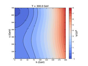
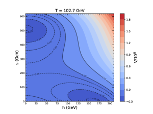
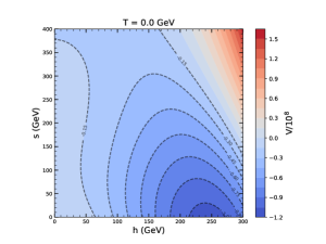
Figure 1: Contours of the effective potential in the $h-s$ plane, with temperature $T=300$ GeV (left), $T=T_{c}$ (middle), and $T=0$ GeV (right), respectively. Here we take the parameters $\lambda_{\chi}=0.5$, $\kappa_{\chi}=0$, $m_{S}=48.9$ GeV, $\theta=-0.258$, $\lambda_{s}=1.54\times 10^{-2}$, $\lambda_{a}=5.25\times 10^{-3}$, $k_{s}=6.31\times 10^{-3}$, $c_{s}=-12.92$ GeV, and $c_{\chi}=32.36$ GeV. The other parameters can be derived from Eq. (3.14) of Ref. Chiang2021JCAP .

In the following, we make use of the scenarios given in Ref. Chiang2020JHEP to search for the parameter space of first-order EWPT with the full one-loop effective potential (3). Note that the parameters should be chosen so as to guarantee several theoretical bounds, including the tree-level vacuum stability Gonderinger2012PRD , perturbativity, and perturbative unitarity Kanemura2016NPB . The most relevant experimental constraints are from the Higgs signal strength observations. We further require the $h-s$ mixing angle $|\theta|\lesssim 0.4$ to be in agreement with these constraints Chiang2020JHEP .

Nucleation temperature – The DM phenomenology of the model has been studied in detail in Ref. Chiang2021JCAP . In this work, we focus on the stochastic gravitational waves emitted from the strong first-order EWPT of the model. A first-order cosmological phase transition begins when the Universe cools down to the critical temperature $T_{c}$, at which point a potential barrier separates the two degenerate phases, the EW symmetry-broken and -unbroken vacua. The stochastic bubble nucleation takes place when the metastable vacuum successfully tunnels into the stable one with the help of thermal fluctuations. The nucleation rate per unit volume and per unit time is approximately given by Apreda2002NPB

$$\Gamma(T)=T^{4}\left(\frac{S_{3}}{2\pi T}\right)^{\frac{3}{2}}e^{-\frac{S_{3}}{T}}~{},$$ (8)

where the three-dimensional on-shell Euclidean action for a spherical bubble configuration can be written as follows

$$S_{3}(T)=4\pi\int drr^{2}\left[\frac{1}{2}\left(\frac{d\phi}{dr}\right)^{2}+V_{\mathrm{eff}}(\phi,T)\right]~{}.$$ (9)

In order to obtain the Euclidean action, we need to know the bubble profile which can be determined by numerically solving the following equation of motion

$$\frac{{d}^{2}\phi}{{d}r^{2}}+\frac{2}{r}\frac{{d}\phi}{{d}r}=\frac{\partial V_{\mathrm{eff}}}{\partial\phi},\quad{\rm with}\quad\phi^{\prime}(0)=0\quad{\rm and}\quad\phi(\infty)=0~{}.$$ (10)

We employ the CosmoTransitions 2.0.2 package CosmoTransitions2012 to perform such numerical calculations of the bubble profile and Euclidean action.

The temperature $T_{*}$ at which the GWs are most violently generated from the first-order phase transition can be approximated to be the nucleation temperature $T_{n}$, $T_{*}\simeq T_{n}$. Note that the bubble nucleation proceeds efficiently when the bubbles are not diluted by the expansion of the Universe. Thus, we can determine the nucleation temperature $T_{n}$ at which the bubble nucleation rate catches up with the Hubble expansion rate, i.e., $\Gamma(T_{n})\simeq H(T_{n})^{4}$. Here in a radiation dominated Universe the Hubble parameter is given by $H=1.66g_{*}^{1/2}T^{2}/M_{\mathrm{pl}}$, with $g_{*}\simeq 110$ and $M_{\mathrm{pl}}=1.22\times 10^{19}~{}\mathrm{GeV}$. This condition is well approximated by $S_{3}(T_{n})/T_{n}\simeq 140$ for the phase transition occuring at the EW-scale temperature of $T\sim\mathcal{O}(100)$ GeV. The criterion of bubble nucleation determines whether the first-order cosmological phase transition has successfully taken place or not.

Gravitational waves – In order to determine the stochastic GW spectrum produced from a first-order phase transition, we need to calculate the following two characteristic parameters Kamionkowski1994PRD

$$\alpha=\frac{\epsilon\left(T_{*}\right)}{\rho_{\operatorname{rad}}\left(T_{*}\right)}~{}\text{ and }~{}\frac{\beta}{H_{*}}=\left.T_{*}\frac{d}{dT}\left(\frac{S_{3}(T)}{T}\right)\right|_{T=T_{*}}~{},$$ (11)

where $\rho_{\mathrm{rad}}=\pi^{2}g_{*}T^{4}/30$ is the radiation energy density in the plasma, and the latent heat associated with the phase transition is $\epsilon(T)=T\partial\Delta V_{bs}(T)/\partial T-\Delta V_{bs}(T)$, with $\Delta V_{bs}(T)$ the potential difference between the EW broken and symmetric phases. The parameter $\alpha$ characterizes the strength of a phase transition. Usually, $\alpha\lesssim 1$ for a typical phase transition without a large amount of supercooling. The parameter $\beta$ defines the time variation of the nucleation rate, and thus $\beta/H_{*}$ dictates the characteristic frequency of the GW spectrum.

It has been shown that bubble collisions, sound waves and turbulence produced after the bubble collisions can be the sources of GW radiations during the percolation of bubbles, leading to the total GW spectrum Caprini2016JCAP $h^{2}\Omega_{\mathrm{GW}}\simeq h^{2}\Omega_{\mathrm{col}}+h^{2}\Omega_{\mathrm{sw}}+h^{2}\Omega_{\mathrm{turb}}$. However, recent studies indicate that bubble collisions provide a negligible contribution to the final GW signal as very little energies are deposited in the bubble walls. In what follows, we will restrict ourselves to the case of non-runaway bubbles, where the GWs can be effectively produced by the sound waves and turbulence.

The GW spectra from sound waves and turbulence are summarized as follows Caprini2016JCAP ; Cai2017JCAP :

$$h^{2}\Omega_{\mathrm{sw}}(f)=2.65\times 10^{-6}\left(\frac{H_{*}}{\beta}\right)\left(\frac{\kappa_{\mathrm{sw}}\alpha}{1+\alpha}\right)^{2}\left(\frac{100}{g_{*}}\right)^{\frac{1}{3}}v_{w}\left(\frac{f}{f_{\mathrm{sw}}}\right)^{3}\left(\frac{7}{4+3\left(f/f_{\mathrm{sw}}\right)^{2}}\right)^{7/2}~{},$$ (12)

$$h^{2}\Omega_{\mathrm{turb}}(f)=3.35\times 10^{-4}\left(\frac{H_{*}}{\beta}\right)\left(\frac{\kappa_{\mathrm{turb}}\alpha}{1+\alpha}\right)^{\frac{3}{2}}\left(\frac{100}{g_{*}}\right)^{1/3}v_{w}\frac{\left(\frac{f}{f_{\mathrm{turb}}}\right)^{3}}{\left(1+\frac{f}{f_{\mathrm{turb}}}\right)^{\frac{11}{3}}\left(1+\frac{8\pi f}{H_{0}}\right)}~{},$$ (13)

where $f_{\mathrm{sw}}=1.9\times 10^{-2}\mathrm{mHz}\frac{1}{v_{w}}\left(\frac{\beta}{H_{*}}\right)\left(\frac{T_{*}}{100\mathrm{GeV}}\right)\left(\frac{g_{*}}{100}\right)^{\frac{1}{6}}$ is the red-shifted peak frequency of the GW spectrum from sound waves and $f_{\text{turb }}=2.7\times 10^{-2}\mathrm{mHz}\frac{1}{v_{w}}\left(\frac{\beta}{H_{*}}\right)\left(\frac{T_{*}}{100\mathrm{GeV}}\right)\left(\frac{g_{*}}{100}\right)^{\frac{1}{6}}$ is the peak frequency for turbulence, $H_{0}=16.5\times 10^{-3}\mathrm{mHz}\left(\frac{T_{*}}{100\mathrm{GeV}}\right)\left(\frac{g_{*}}{100}\right)^{\frac{1}{6}}$ is the red-shifted Hubble constant, $v_{w}$ denotes the bubble wall velocity and is assigned to be around unity. The efficiency factors $\kappa_{\mathrm{sw}}$ and $\kappa_{\mathrm{turb}}$ indicate respectively the fractions of latent heat that are transformed into the bulk motion of the plasma and the turbulence, in both of which the energy density finally goes into the emission of GWs. For non-runaway bubbles with $v_{w}\sim 1$, the efficiency factors satisfy $\kappa_{\mathrm{sw}}\simeq\alpha/(0.73+0.083\sqrt{\alpha}+\alpha)$ and $\kappa_{\text{turb }}=\epsilon\kappa_{\text{sw }}$, where we take $\epsilon=0.1$ in this work. Note that the amplitude of the GW spectrum visible today is further suppressed by a factor of $\Upsilon=1-1/\sqrt{1+2\tau_{\mathrm{sw}}H_{s}}$ Guo2021JCAP . We recommend Refs. Guo2021JCAP ; Hindmarsh2021SPLN ; Ellis2021JCAP for more details about recent developments toward understanding the GW production from first-order cosmological phase transitions.

Signal-to-noise ratio – With the frequentist approach, the detectability of the stochastic GW signals is measured by the corresponding signal-to-noise ratio (SNR) Caprini2016JCAP

$$\rho=\sqrt{\mathcal{N}\mathcal{T}_{\mathrm{obs}}\int_{f_{\min}}^{f_{\max}}df\left[\frac{h^{2}\Omega_{\mathrm{GW}}(f)}{h^{2}\Omega_{\exp}(f)}\right]^{2}}~{},$$ (14)

where $\mathcal{N}$ is the number of independent observatories of an experiment. For example, $\mathcal{N}=1$ for the auto-correlated experiments like LISA LISA2017 ; Robson2019CQG and B-DECIGO Seto2001PRL ; Isoyama2018PTEP , while $\mathcal{N}=2$ for the cross-correlated experiments such as DECIGO Sato2017JPCS and BBO Crowder2005PRD . $\mathcal{T}_{\text{obs }}$ is the duration of the mission in units of year. Here we assume a mission duration of $\mathcal{T}_{\text{obs }}=4$ years for all of the experiments. $h^{2}\Omega_{\rm exp}$ denotes the sensitivity of a GW experiment, which is summarized in appendix E of Ref. Chiang2020JHEP , where we also give the associated experimental frequency ranges ($f_{\rm min}-f_{\rm max}$) Hz in Table 2. We adopt the commonly used SNR threshold $\rho_{\rm thr}=10$, above which the GW signal can be regarded as detectable by one experiment.

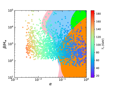
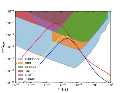
Figure 2: Left: the colored regions represent the parameter space with a SNR $\rho>\rho_{\rm thr}$ for LISA (orange), B-DECIGO (light-green), DECIGO (light-blue), and BBO (pink) experiments. The scatter points denote the scenarios that can both generate a strong first-order EWPT and have a correct DM relic density $h^{2}\Omega_{\rm DM}\simeq 0.12$. The colorbar for the scatters denotes the nucleation temperature $T_{n}$, in units of GeV. Right: GW spectra from the phase transition (curves) and various experimental sensitivities (colored patches) as a function of frequency. The yellow, blue, and red curves represent the results in scenarios A, B, and C as summarized in Table 1. Furthermore, these scenarios give a correct DM relic density 0.12. Scenario A with a spin-independent DM-nucleon elastic scattering cross section $\sigma_{\rm SI}=1.27\times 10^{-46}$ $\rm cm^{2}$ and scenario B with $\sigma_{\rm SI}=1.23\times 10^{-47}$ $\rm cm^{2}$ survive the XENON1T XENON1T2018PRL and PandaX PandaX-II2017PRL constraints and are testable in the future XENONnT experiment, as well as the BBO and U-DECIGO GWs detections. Scenario C with $\sigma_{\rm SI}=5.70\times 10^{-48}$ $\rm cm^{2}$ is beyond the future XENONnT XENONnT2016JCAP experimental sensitivity, however its GW signal is detectable for the LISA, Taiji, and TianQin experiments. We have also checked that the DM candidate $\chi$ of these models has a total annihilation cross section $\langle\sigma v\rangle_{\rm tot}\simeq 2.2\times 10^{-26}$ $\rm cm^{3}/s$ (see Table 2), which is much lower than the upper limits on the DM annihilation to SM particles from Fermi-LAT Fermi2015PRL and MAGIC MAGIC2016JCAP gamma-ray observations of dwarf satellite galaxies.

Table 1: Summary of scenarios used in the right plot Fig. 2, assuming $\lambda_{\chi}=0.5$ and $\kappa_{\chi}=0$.

Scenario	$m_{S}$/GeV	$m_{\chi}$/GeV	$\theta$	$\lambda_{a}$	$c_{\chi}$/GeV	$\lambda_{s}$	$\kappa_{s}$	$c_{s}$/GeV	$\lambda_{h}$
A	182.0	1524.0	0.342	0.467	$-403.0$	1.3	0.21	$-367.0$	0.145
B	109.0	984.0	0.279	0.309	162.0	0.71	0.451	$-135.0$	0.127
C	137.0	1887.1	0.228	0.581	$-478.0$	0.85	0.403	$-200.0$	0.130

Table 2: Summary of results for the three scenarios given in Table 1.

Scenario	$\sigma_{\rm SI}$/${\rm cm^{2}}$	$\langle\sigma v\rangle_{\rm tot}$/${\rm cm^{3}s^{-1}}$	$v_{c}/T_{c}$	$T_{c}$/GeV	$w_{c}$/GeV	$T_{n}$/GeV	$\beta/H_{*}$	$\alpha$
A	$1.27\times 10^{-46}$	$2.17\times 10^{-26}$	1.32	173.0	194.7	53.57	1343.0	0.139
B	$1.23\times 10^{-47}$	$2.16\times 10^{-26}$	1.10	196.3	186.2	55.96	1680.8	0.112
C	$5.70\times 10^{-48}$	$2.17\times 10^{-26}$	1.13	193.4	192.6	38.37	512.8	0.523

We present our main results in Fig. 2. The colored regions of the left plot denote the detectable parameter spaces for LISA (orange), B-DECIGO (light-green), DECIGO (light-blue), and BBO (pink). As illustrated above, we follow the scenario provided in Ref. Chiang2020JHEP to search for the first-order EWPT for the one-loop potential (3) and take into account the constraints from vacuum stability, perturbativity, and perturbative unitarity as well as the Higgs signal strength observations, as done in Refs. Chiang2020JHEP ; Chiang2021JCAP . We then check the bubble nucleation criterion and calculate the GW parameters with the help of CosmoTransitions 2.0.2 CosmoTransitions2012 . Furthermore, the DM phenomenology including the DM relic density as well as direct detection cross sections has also been investigated using the MicrOMEGAs 5.0.4 package MicrOMEGAs2018CPC in which the model is implemented with the FeynRules 2.3 package FeynRules2014CPC . All the scattering points depicted in the left plot further have the correct DM relic density $h^{2}\Omega_{\rm DM}\simeq 0.12$ as obtained by the Planck observations Planck2016 in the $\Lambda$CDM framework. More interestingly, some of the above DM benchmarks with the correct DM relic density can even evade the current stringent constraints from DM direct and indirect searches. We select three scenarios with their parameters given in Table 1, while the numerical predictions of some important DM and GW quantities for each model are presented in Table 2. The GW signals from the first-order EWPT in these selected scenarios are depicted in the right plot of Fig. 2. We observe that these signals have both the appropriate peak frequencies and the sufficient amplitudes, so they are suitable targets for LISA LISA2017 ; Robson2019CQG , Taiji Hu2017NSR ; Ruan2020NA , TianQin Luo2016CQG ; Hu2018CAG , BBO Crowder2005PRD , and U-DECIGO Kudoh2006PRD experiments. Therefore, as demonstrated with this simple complex-singlet-scalar extended model, the future space-based GW observations provide us an important new tool to probe the DM physics.

Summary – Although the WIMP with mass around 1 TeV is one of the most popular DM scenarios, in recent years it suffers from grave challenges from DM direct detections, cosmic ray observations, and collider searches. In fact, previous works have shown that the singlet extensions of Higgs portal WIMP models with a $Z_{2}$ or $U(1)$ symmetry have already been well constrained by the XENON1T experiment as well as the Fermi-LAT gamma-ray measurements. We have found in Ref. Chiang2021JCAP that by extending to the $CP$ symmetry, it is possible for the singlet extension model to trigger a strong first-order EWPT and to provide a correct DM relic abundance while evading various constraints from DM experiments. In this work, we focus on studying the stochastic gravitational-wave signals emitted from a strong first-order EWPT in such a model. We show that there are ample parameter samples that can give rise to a correct DM relic abundance while generating a significant stochastic GW background, which can be probed by near-future space-based GW experiments, including BBO, U-DECIGO, LISA, Taiji, and TianQin. Among these model samples, we identify three benchmarks with the DM mass $\sim 1$ TeV and the total annihilation cross section $\simeq 2\times 10^{-26}$ ${\rm cm^{3}/s}$. Two of them are testable by the future XENONnT underground DM experiment, while the GW signals from all three benchmarks are sufficiently loud for upcoming space-based GW observations. By this simple model example, we hope to demonstrate that the GW measurement provides us a new way to detect and probe the nature of DM, complementary to the traditional detection methods.

Acknowledgments – BQL is supported in part by the Huzhou University under startup Grant No. RK21094 and National Natural Science Foundation of China (NSFC) under Grant No. 12147219. CWC is supported in part by the Ministry of Science and Technology of Taiwan under Grant No. MOST-108-2112-M-002-005-MY3. DH is supported in part by the National Key Research and Development Program of China under Grant No. 2021YFC2203003, National Natural Science Foundation of China (NSFC) under Grant No. 12005254 and the Key Research Program of Chinese Academy of Sciences under grant No. XDPB15.

References

- (1) Planck collaboration, Planck 2015 results. XIII. Cosmological parameters, Astron. Astrophys. 594 (2016) A13 [arXiv:1502.01589].
- (2) V. C. Rubin and W. K. Ford Jr., Rotation of the Andromeda nebula from a spectroscopic survey of emission regions, Astrophys. J. 159 (1970) 379.
- (3) B. W. Lee and S. Weinberg, Cosmological lower bound on heavy-neutrino masses, Phys. Rev. Lett. 39 (1977) 165.
- (4) P. Hut, Limits on masses and number of neutral weakly interacting particles Phys. Lett. 69B (1977) 85.
- (5) D. J. Weir, Gravitational waves from a first order electroweak phase transition: a review, Phil. Trans. Roy. Soc. Lond. A 376 (2018) 20170126.
- (6) R.-G. Cai, K. Hashino, S.-J. Wang, and J.-H. Yu, Gravitational waves from patterns of electroweak symmetry breaking: an effective perspective, [arXiv:2202.08295].
- (7) LISA Collaboration, Laser Interferometer Space Antenna, [arXiv:1702.00786].
- (8) W. R. Hu and Y. L. Wu, The Taiji Program in Space for gravitational wave physics and the nature of gravity, Natl. Sci. Rev. 4 (2017) 685.
- (9) W. H. Ruan, C. Liu, Z. K. Guo, Y. L. Wu and R. G. Cai, The LISA–Taiji network, Nature Astronomy 4 (2020) 108–109. [arXiv:2008.2002.03603].
- (10) J. Luo et al. [TianQin Collaboration], TianQin: a space-borne gravitational wave detector, Class. Quant. Grav. 33 (2016) 035010 [arXiv:1512.02076].
- (11) X. C. Hu et al., Fundamentals of the orbit and response for TianQin, Class. Quant. Grav. 35 (2018) 095008 [arXiv:1803.03368].
- (12) J. Crowder and N. J. Cornish, Beyond LISA: Exploring future gravitational wave missions, Phys. Rev. D 72 (2005) 083005 [gr-qc/0506015].
- (13) N. Seto, S. Kawamura and T. Nakamura, Possibility of direct measurement of the acceleration of the universe using 0.1-Hz band laser interferometer gravitational wave antenna in space, Phys. Rev. Lett. 87 (2001) 221103 [astro-ph/0108011].
- (14) V. A. Kuzmin, V. A. Rubakov and M. E. Shaposhnikov, On the Anomalous Electroweak Baryon Number Nonconservation in the Early Universe, Phys. Lett. B155 (1985) 36.
- (15) A. G. Cohen, D. B. Kaplan and A. E. Nelson, Weak scale baryogenesis, Phys. Lett. B245 (1990) 561.
- (16) D. E. Morrissey and M. J. Ramsey-Musolf, Electroweak baryogenesis, New J. Phys. 14 (2012) 125003 [arXiv:1206.2942].
- (17) M. D’Onofrio, K. Rummukainen, and A. Tranberg, Sphaleron Rate in the Minimal Standard Model, Phys. Rev. Lett. 113, (2014) 141602. [arXiv:1404.3565].
- (18) T. Alanne et al., Pseudo-Goldstone dark matter: gravitational waves and direct-detection blind spots, JHEP 10 (2020) 080 [arXiv:2008.09605].
- (19) C.-W. Chiang, D. Huang, and B.-Q. Lu Electroweak phase transition confronted with dark matter detection constraints, JCAP 01 (2021) 035. [arXiv:2009.08635]
- (20) J. M. Cline and K. Kainulainen, Electroweak baryogenesis and dark matter from a singlet Higgs, JCAP 01 (2013) 012 [arXiv:1210.4196].
- (21) W. L. Guo and Y. L. Wu, The real singlet scalar dark matter model, JHEP 10 (2010) 083 [arXiv:1006.2518].
- (22) M.J. Ramsey-Musolf, The Electroweak Phase Transition: A Collider Target, [arXiv:1912.07189].
- (23) K Hashino, M Kakizaki, S Kanemura, P. Ko and T. Matsui, Gravitational waves from first order electroweak phase transition in models with the gauge symmetry, JHEP 06 (2018) 088 [arXiv:1802.02947].
- (24) K Kannike, M Raidal, Phase transitions and gravitational wave tests of pseudo-Goldstone dark matter in the softly broken scalar singlet model, Phys. Rev. D 99 (2019) 115010 [arXiv:1901.03333].
- (25) L. Feng, S. Profumob and L. Ubaldi, Closing in on singlet scalar dark matter: LUX, invisible Higgs decays and gamma-ray lines, JHEP 03 (2015) 045. [arXiv:1412.1105].
- (26) S.R. Coleman and E.J. Weinberg, Radiative Corrections as the Origin of Spontaneous Symmetry Breaking, Phys. Rev. D 7 (1973) 1888.
- (27) C. W. Chiang and B. Q. Lu, First-order electroweak phase transition in a complex singlet model with symmetry, JHEP 07 (2020) 082 [arXiv:1912.12634].
- (28) H. H. Patel and M. J. Ramsey-Musolf, Baryon Washout, Electroweak Phase Transition, and Perturbation Theory, JHEP 1107 (2011) 029 [arXiv:1101.4665].
- (29) C. W. Chiang, M. J. Ramsey-Musolf and E. Senaha, Standard model with a complex scalar singlet: Cosmological implications and theoretical considerations, Phys. Rev. D 97 (2018) 015005. [arXiv:1707.09960].
- (30) M. Gonderinger, H. Lim and M. J. Ramsey-Musolf, Complex scalar singlet dark matter: Vacuum stability and phenomenology, Phys. Rev. D 86 (2012) 043511. [arXiv:1202.1316].
- (31) S. Kanemura, M. Kikuchi and K. Yagyu, Radiative corrections to the Higgs boson couplings in the model with an additional real singlet scalar field, Nucl. Phys. B 907 (2016) 286 [arXiv:1511.06211].
- (32) R. Apreda, M. Maggiore, A. Nicolis and A. Riotto, Gravitational waves from electroweak phase transitions, Nucl. Phys. B 631 (2002) 342 [gr-qc/0107033].
- (33) C.L. Wainwright, CosmoTransitions: Computing Cosmological Phase Transition Temperatures and Bubble Profiles with Multiple Fields, Comput. Phys. Commun. 183 (2012) 2006 [arXiv:1109.4189].
- (34) M. Kamionkowski, A. Kosowsky and M.S. Turner, Gravitational radiation from first order phase transitions, Phys. Rev. D 49 (1994) 2837 [astro-ph/9310044].
- (35) C. Caprini et al., Science with the space-based interferometer eLISA. II: Gravitational waves from cosmological phase transitions, JCAP 04 (2016) 001 [arXiv:1512.06239].
- (36) R.-G. Cai, M. Sasaki and S.-J. Wang, The gravitational waves from the first-order phase transition with a dimension-six operator, JCAP 08 (2017) 004 [arXiv:1707.03001].
- (37) H.-K. Guo, K. Sinha, D. Vagie and G. White, Phase Transitions in an Expanding Universe: Stochastic Gravitational Waves in Standard and Non-Standard Histories, JCAP 01 (2021) 001 [arXiv:2007.08537].
- (38) M.B. Hindmarsh, M. Lben, J. Lumma and M. Pauly, Phase transitions in the early universe, SciPost Phys. Lect. Notes 24 (2021) 1 [arXiv:2008.09136].
- (39) J. Ellis, M. Lewicki and J.M. No, On the Maximal Strength of a First-Order Electroweak Phase Transition and its Gravitational Wave Signal, JCAP 04 (2019) 003 [arXiv:1809.08242].
- (40) T. Robson, N.J. Cornish and C. Liu, The construction and use of LISA sensitivity curves, Class. Quant. Grav. 36 (2019) 105011 [arXiv:1803.01944].
- (41) S. Isoyama, H. Nakano and T. Nakamura, Multiband Gravitational-Wave Astronomy: Observing binary inspirals with a decihertz detector, B-DECIGO, PTEP 2018 (2018) 073E01 [arXiv:1802.06977]
- (42) S. Sato et al., The status of DECIGO, J. Phys. Conf. Ser. 840 (2017), 012010.
- (43) XENON Collaboration, Dark Matter Search Results from a One Ton-Year Exposure of XENON1T, Phys. Rev. Lett. 121 (2018) 111302. [arXiv:1805.12562].
- (44) PandaX-II Collaboration, Dark Matter Results from 54-Ton-Day Exposure of PandaX-II Experiment, Phys. Rev. Lett. 119 (2017) 181302. [arXiv:1708.06917].
- (45) XENON Collaboration, Physics reach of the XENON1T DM experiment, JCAP 04 (2016) 027 [arXiv:1512.07501].
- (46) M. Ackermann et al. Fermi-LAT collaboration, Searching for Dark Matter Annihilation from Milky Way Dwarf Spheroidal Galaxies with Six Years of Fermi Large Area Telescope Data, Phys. Rev. Lett. 115 (2015) 231301 [arXiv:1503.02641].
- (47) M.L. Ahnen et al., Limits to dark matter annihilation cross-section from a combined analysis of MAGIC and Fermi-LAT observations of dwarf satellite galaxies, JCAP 02 (2016) 039 [arXiv:1601.06590].
- (48) D. Barducci et al., Collider limits on new physics within MicrOMEGAs 4.3, Comput. Phys. Commun. 222 (2018) 327 [arXiv:1606.03834].
- (49) A. Alloul, N. D. Christensen, C. Degrande, C. Duhr, and B. Fuks, FeynRules 2.0 - A complete toolbox for tree-level phenomenology, Comput. Phys. Commun. 185 (2014) 8 [arXiv:1310.1921].
- (50) H. Kudoh, A. Taruya, T. Hiramatsu and Y. Himemoto, Detecting a gravitational-wave background with next-generation space interferometers, Phys. Rev. D 73, (2006) 064006 [gr-qc/0511145].