Individualized Risk Assessment of Preoperative Opioid Use by Interpretable Neural Network Regression

Abstract

Preoperative opioid use has been reported to be associated with higher preoperative opioid demand, worse postoperative outcomes, and increased postoperative healthcare utilization and expenditures. Understanding the risk of preoperative opioid use helps establish patient-centered pain management. In the field of machine learning, deep neural network (DNN) has emerged as a powerful means for risk assessment because of its superb prediction power; however, the blackbox algorithms may make the results less interpretable than statistical models. Bridging the gap between the statistical and machine learning fields, we propose a novel Interpretable Neural Network Regression (INNER), which combines the strengths of statistical and DNN models. We use the proposed INNER to conduct individualized risk assessment of preoperative opioid use. Intensive simulations and an analysis of 34,186 patients expecting surgery in the Analgesic Outcomes Study (AOS) show that the proposed INNER not only can accurately predict the preoperative opioid use using preoperative characteristics as DNN, but also can estimate the patient-specific odds of opioid use without pain and the odds ratio of opioid use for a unit increase in the reported overall body pain, leading to more straightforward interpretations of the tendency to use opioids than DNN. Our results identify the patient characteristics that are strongly associated with opioid use and is largely consistent with the previous findings, providing evidence that INNER is a useful tool for individualized risk assessment of preoperative opioid use.

Keywords deep learning  $\cdot$ pain research  $\cdot$ precision medicine  $\cdot$ generalized linear models

1 Introduction

The drastic increase in the use of opioids has led to an epidemic in the U.S., with more than 46,000 estimated overdose deaths in 2018 [Brown et al. (2021)]. As an effort to combat this crisis, researchers have begun to study preoperative opioid use because it is a major factor associated with opioid misuse [Saha et al. (2016)], higher postoperative opioid demand [Armaghani et al. (2014); Schoenfeld et al. (2018)], worse postoperative outcomes [Lee et al. (2014); Smith et al. (2017); Morris et al. (2016); Jain et al. (2018)], and increased postoperative healthcare utilization and expenditures [Cron et al. (2017); Waljee et al. (2017); Jain et al. (2018)]. Understanding preoperative opioid use among patients expecting surgical services can help surgeons establish effective pain management for patients [Hilliard et al. (2018)], including postoperative opioid management  [Roeckel et al. (2016)].

What has often been overlooked is that a sizeable portion of patients consumed opioids preoperatively even with no reported pains  [Roeckel et al. (2016)], which might hint at possible opioid misuse. As part of the Analgesic Outcomes Study (AOS)  [Brummett et al. (2013)], a large observational cohort study investigating associations between preoperative pain and opioid use, individualized risk of preoperative opioid use is assessed to identify patients who tend to use preoperative opioids even when there is little pain as well as those who tend to take preoperative opoids even when the pain increases only slightly  [Brummett et al. (2015)]. With opioid use (yes or no) as the outcome and pain level as the covariate, a logistic regression model with an intercept and a slope that depend on patients’ other characteristics may help delineate the subgroups of patients who are at high risks of opioids misuse; see model (1). However, because of the curse of dimensionality, traditional nonparametric methods of fitting varying coefficient logistic models may not fare well [Park et al. (2015); Hastie and Tibshirani (1993); Cai et al. (2000)], even when the number of patient characteristics is only moderately large.

On the other hand, deep neural network (DNN), a machine learning algorithm inspired by the structure of brains, has achieved much success in nonparametric approximation with high dimensional predictors [Bauer and Kohler (2019); Schmidt-Hieber (2020)]. It has found applications in computational phenotyping [Che et al. (2015); Lipton et al. (2015)], medical imaging analysis [Kleesiek et al. (2016); Tran (2016)] and predictive modeling [Choi et al. (2016)], among many others. It is challenging to explain the decision rules of DNN with the input variables, due to the black-box nature; directly applying DNN to the aforementioned AOS data cannot pinpoint the subgroup of patients who may be at high risks of opioid misuse.

For example, Dong et al. (2019) use the Gini importance index from the random forest model to rank features, while Lo-Ciganic et al. (2019) use the boosting decision tree. However, neither of these methods can give the direction of the association between features and opioid dependence. On the other hand, Che et al. (2017) use a weight matrix of each layer in the DNN model to generate “importance scores” to detect important features. The scores not only rank different features in terms of opioid overdose prediction but also inform the direction of the association. However, the method may not directly decipher the relationship between opioid use and pain, or, in particular, identify subpopulations who are likely to be sensitive to pain or be opioid dependent even without reported pains.

Bridging the gap between the statistical and machine learning fields, we propose an interpretable neural network regression (INNER) that combines the strengths of logistic regression and DNN models. We propose a logistic regression model with individualized coefficients, wherein the regression coefficients are functions of individual characteristics. We utilize DNN to estimate these individualized coefficients and construct two metrics, Baseline Opioid Tendency (BOT) and Pain-induced Opioid Tendency (POT), which are useful for the individualized assessment of opioid use for each patient. In particular, BOT refers to the odds of using preoperative opioids when the patient does not report pain and POT is the odds ratio of using preoperative opioids for a unit increase in the reported overall body pain. These two metrics can be used to identify subgroups of patients, whose characteristics are associated with preoperative opioid use: patients with high POT are more likely to get preoperative opioids when pain increases, and patients with high BOT have a high risk of preoperative opioid use even with no reported pain. To demonstrate the utility of our proposal, we conduct simulations and apply the INNER model to analyze the AOS study. Our analysis identifies patient characteristics that are associated with opioid tendency, as quantified by BOT and POT, and is largely consistent with the literature, evidencing the usefulness of INNER for individualized risk assessment of preoperative opioid use.

2 Review of a Deep Neural Network

A DNN has multiple layers with neurons being the basic processing units [LeCun et al. (2015)]. For example, in the commonly used feedforward neural network [Shrestha and Mahmood (2019)], starting from the first layer (input layer), neurons in one layer are connected to and may “activate” those in the adjacent and higher layers. Specifically, the inputs of each neuron are multiplied by some weights, added with respective bias terms and summed up [Shrestha and Mahmood (2019); Fan et al. (2021)]. The sums are passed onto some transformation functions, called “activation” functions, such as linear, Sigmoid, hyperbolic tangent or rectified linear unit (ReLU) activation functions [Karlik and Olgac (2011); Li and Yuan (2017)]. The outputs returned by these activation functions are fed to neurons in the next layer as inputs. Passing all of the layers, the outputs of the final layer (output layer) will be used for prediction.

3 Interpretable Neural Network Regression

Our proposed INNER model is a logistic regression model with covariate-dependent coefficient functions constructed by DNN. The general formulation is similar to that of a DNN. Specifically, let $\mathbb{R}^{d}$ be a $d$-dimensional Euclidean vector space. To construct a prediction based on input $\mathbf{x}\in\mathbb{R}^{k_{l}}$ via a neural network with $L$ layers, where the $l$th ($l=1,\ldots,L$) layer consists of $k_{l}$ neurons, we adopt an $L$-fold composite function $F_{L}:\mathbb{R}^{k_{1}}\to\mathbb{R}^{k_{L+1}}$ with the parameter $\boldsymbol{\theta}$, i.e.,

$$F_{L}(\cdot;\boldsymbol{\theta})=f_{L}\circ f_{L-1}\circ\cdots\circ f_{1}(\cdot),$$

where $f_{l}(\mathbf{x})=\sigma_{l}(\mathbf{W}_{l}\mathbf{x}+\mathbf{b}_{l})\in\mathbb{R}^{k_{l+1}}$ and “$\circ$” indicates the composition of two functions. The function $\sigma_{l}:\mathbb{R}^{k_{l+1}}\to\mathbb{R}^{k_{l+1}}$ is a (non)linear activation function for the $l$th layer. The parameter $\boldsymbol{\theta}=\{\mathbf{W}_{l},\mathbf{b}_{l}\}_{l=1}^{L}$, where $\mathbf{W}_{l}$ is the weight matrix of dimension $k_{l+1}\times k_{l}$ and $\mathbf{b}_{l}\in\mathbb{R}^{k_{l+1}}$ is the bias vector. Typical choices of $\sigma_{l}(\mathbf{x})$ include a linear function of $\mathbf{x}$, a ReLU function, i.e., $\mathrm{max}(0,\mathbf{x})$, and a softmax function, i.e., $\exp(\mathbf{x})/\|\exp(\mathbf{x})\|_{1}$, where max and $\exp$ operate componentwise.

Let $\mathcal{D}=\{(X_{i},\mathbf{Z}_{i},Y_{i}),i=1,\ldots,N\}$ be a dataset consisting of $N$ independent patients. For patient $i\in\{1,\ldots,N\}$, let $Y_{i}\in\{0,1\}$ be a binary variable indicating whether the patient uses opioids preoperatively. Let $X_{i}\in[0,10]$ represent the overall body pain score and $\mathbf{Z}_{i}\in\mathbb{R}^{p}$ represent a vector of $p$ preoperative characteristics. We model the conditional probability of preoperative opioid use given the preoperative characteristics and the overall body pain score via

$$\mathrm{logit}\{\mathrm{P}(Y_{i}=1\mid X_{i},\mathbf{Z}_{i})\}=F_{L}(\mathbf{Z}_{i};\boldsymbol{\alpha})+F_{L}(\mathbf{Z}_{i};\boldsymbol{\beta})\cdot X_{i},$$ (1)

where $\mathrm{logit}(p)=\log\{p/(1-p)\}$, with $p\in(0,1)$, is the logit link function. The two covariate-dependent coefficient functions are constructed by two neural networks with the same network architecture but different parameters: $\boldsymbol{\alpha}$ and $\boldsymbol{\beta}$. Model (1) is termed an INNER model, wherein the number of neurons in the input layer is $k_{1}=p$ and the output layer has only one neuron, i.e., $K_{L+1}=1$. Figure 1 shows an example of three layers ($L=3$), where the first two layers have 250 and 125 hidden neurons, respectively, with a ReLU activation function, and the third layer has one hidden neuron with a linear activation function. During training, we may randomly select a certain number of neurons in a layer and ignore them in order to overcome overfitting [Srivastava et al. (2014)]. The proportion of such ignored neurons in a layer is called the dropout rate with that layer. During testing, dropout is set to be inactive with no neurons ignored.

We use the Sigmoid activation function, i.e., $\mathrm{Sigmoid}(x)=\{1+\exp(-x)\}^{-1},$ for the output layer of the INNER model. Here, $x$ comes from the affine combination of the two sub-networks whose final layers have a linear activation function, and the Sigmoid function returns a value between 0 and 1, ensuring numerical stability. The number of hidden layers, along with the number of hidden neurons and the dropout rate in each layer, are hyperparameters to be selected based on the prediction performance.

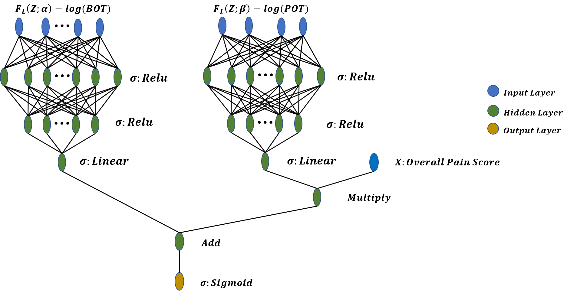
Figure 1: Example of INNER. Input: overall pain score (X) and other characteristics ($\mathbf{Z}$). Two neural networks for $F_{L}(\mathbf{Z};\boldsymbol{\alpha})$ and $F_{L}(\mathbf{Z};\boldsymbol{\beta})$: the same network architecture with different parameters, $\boldsymbol{\alpha}$ and $\boldsymbol{\beta}$; three hidden layers in each network, with the first layer having 250 neurons with a ReLu activation function, the second layer having 125 neurons with a ReLu activation function, and the last layer having one neuron with a linear activation function. Ouput: estimated probability of preoperative opioid use.

Our proposed INNER is interpretable within the traditional logistic regression framework, and can assess the individualized risk of preoperative opioid use via two derived metrics: Baseline Opioid Tendency (BOT), the odds of taking opioid with no reported pain, and Pain-induced Opioid Tendency (POT), the odds ratio of taking opioid for a unit increase in overall body pain. In particular, BOT and POT can be represented by the output of the two neural networks with the input $\boldsymbol{Z}$ respectively:

$$\mbox{Baseline Opioid Tendency (BOT)}\coloneqq\mbox{exp}\{F_{L}(\mathbf{Z};\boldsymbol{\alpha})\},$$

$$\mbox{Pain-induced Opioid Tendency (POT)}\coloneqq\exp\{F_{L}(\mathbf{Z};\boldsymbol{\beta})\}.$$

Therefore, a high Baseline Opioid Tendency (BOT) or a high Pain-induced Opioid Tendency (POT) indicates a potential high risk of taking preoperative opioids.

The estimates of parameters, denoted by $\hat{\boldsymbol{\alpha}}$ and $\hat{\boldsymbol{\beta}}$, are obtained by minimizing the negative log likelihood or the cross entropy loss function

$$\mathcal{L}(\boldsymbol{\alpha},\boldsymbol{\beta};\mathcal{D}) =-\sum_{i=1}^{N}Y_{i}\log\{\mathrm{P}(Y_{i}=1\mid X_{i},\mathbf{Z}_{i})\}+(1-Y_{i})\log\{1-\mathrm{P}(Y_{i}=1\mid X_{i},\mathbf{Z}_{i})\},$$ (2)

where $\mathrm{P}(Y_{i}=1\mid X_{i},\mathbf{Z}_{i})$ is as defined in (1). We use stochastic gradient descent (SGD) [Bottou (2010)] for optimization. In our later data analysis and out of a total of 34,186 patients, we randomly assign 23,931 (70%) patients to be training samples ($\mathcal{T}$) and the rest 10,256 (30%) patients to be validation samples ($\mathcal{V}$) when computing the training and validation loss.

Input: learning rate ($\eta$), maximum difference ($\Delta$), batch size ($M$)

Output: $\hat{\boldsymbol{\alpha}}$, $\hat{\boldsymbol{\beta}}$

Data: Partition full data $\mathcal{D}$ to training ($\mathcal{T}$) and validation ($\mathcal{V}$) samples

Initialization $\boldsymbol{\alpha}^{0}$, $\boldsymbol{\beta}^{0}$, training loss = validation loss

while validation loss - training loss $\leq$ $\Delta$ do

       for mini-batch $m\leftarrow 1$ to $M$ do

             Draw random samples without replacement $(X_{i},\mathbf{Z}_{i},Y_{i})\in\mathcal{T}$

       end for

      Compute gradients $\nabla_{\boldsymbol{\alpha}}\mathcal{L}$ and $\nabla_{\boldsymbol{\beta}}\mathcal{L}$ of mini-batch

       Update parameters $\boldsymbol{\alpha}=\boldsymbol{\alpha}-\eta\nabla_{\boldsymbol{\alpha}}\mathcal{L}$ and $\boldsymbol{\beta}=\boldsymbol{\beta}-\eta\nabla_{\boldsymbol{\beta}}\mathcal{L}$

       Compute training loss: $\mathcal{L}(\boldsymbol{\alpha},\boldsymbol{\beta};\mathcal{T})$

       Compute validation loss: $\mathcal{L}(\boldsymbol{\alpha},\boldsymbol{\beta};\mathcal{V})$

      

end while

Algorithm 1 Stochastic Gradient Descent

In general, classical stochastic gradient descent is sensitive to the choice of learning rates; a large learning rate gives fast convergence but may induce numerical instability [Liu et al. (2020); Darken et al. (1992)], while a small learning rate may ensure stability, though at the price of more iterative steps. In our implementation, we use grid search to tune the learning rates. For the real data analysis, we tune the learning rate over the range between 0.005 to 0.1 with 20 equally spaced grid points, and set the batch size to be 64 and the maximum difference between the training and validation loss to be $10^{-2}$. We obtain the estimates, $\hat{\boldsymbol{\alpha}}$ and $\hat{\boldsymbol{\beta}}$, after 200 iterations. We also conduct sensitivity analysis to assess the robustness of SGD towards the choices of these hyperparameters, and find the model’s predictiveness performance is fairly robust to them; see Appendix B.

With $\hat{\boldsymbol{\alpha}}$ and $\hat{\boldsymbol{\beta}}$, BOT and POT can be estimated by plugging in these estimates: for a patient with $\mathbf{Z}_{i}$, the estimated BOT and POT are $\mbox{exp}\{F_{L}(\mathbf{Z}_{i};\hat{\boldsymbol{\alpha}})\}$ and $\mbox{exp}\{F_{L}(\mathbf{Z}_{i};\hat{\boldsymbol{\beta}})\}$, respectively.

4 Simulation Study

We compare the prediction power and robustness of the proposed INNER with the existing methods, including decision trees, random forests, Bayesian additive regression trees regression (BART), support vector machine (SVM), logistic regression and DNN. Under various scenarios examined, we find that INNER outperform these competing methods. The prediction power of INNER is similar to or even better than DNN when the model assumptions of INNER hold, whereas INNER achieves a performance comparable to DNN even when the model assumptions are violated. Codes for the simulation study are provided in the Supplementary Material.

4.1 Prediction Power

We simulate data from a logistic regression model with non-linear varying-coefficient functions:

$$\mathrm{logit}\{\mathrm{P}(Y=1\mid X,\mathbf{Z})\}=\sin(\mathbf{Z}^{\top}\boldsymbol{\alpha})+\cos(\mathbf{Z}^{\top}\boldsymbol{\beta})\cdot X.$$

The simulation study is designed with varying signal strengths, noise variances, number of covariates and sample sizes. The signal strength is measured by a signal-to-noise ratio, i.e.,

$$\frac{\mathrm{Var}\{\mathrm{P}(Y=1\mid X,\mathbf{Z})\}}{\mathrm{Var}(Y)-\mathrm{Var}\{\mathrm{P}(Y=1\mid X,\mathbf{Z})\}}.$$

We assess the prediction power of INNER by varying the signal-to-noise ratio to be 0.2, 0.8 or 3.2, and setting the sample size and the number of signal covariates to be 40,000 and 16, respectively.

We next increase the noise variance by adding various numbers of noise covariates (8, 12 and 16) into the data, while fixing the signal-to-noise ratio, the number of samples and the number of covariates at 3.2, 40,000 and 16 respectively. We finally consider several combinations of the numbers of covariates (9, 16, 32) and samples (5,000; 10,000; 20,000), with a signal-to-noise ratio of 3.2 and in the absence of noise covariates.

For each simulation configuration, we conduct a total of 500 experiments. In each experiment, we randomly allocate 80% of the samples to the training data and the rest to the testing data, and compare seven methods: the INNER model [equation (1)], DNN, decision trees, random forests, BART and SVM models with combined $\mathbf{Z}$ and $X$ as the input, and the logistic regression model with a two-way interaction between $\mathbf{Z}$ and $X$. For the logistic regression, we present it as a special case of INNER with only one layer and a linear activation function, that is,

$$\mathrm{logit}\{\mathrm{P}(Y=1\mid X,\mathbf{Z})\}=\mathbf{Z}^{\top}\mathbf{W}_{\alpha}+b_{\alpha}+(\mathbf{Z}^{\top}\mathbf{W}_{\beta}+b_{\beta})\cdot X,$$ (3)

where $\mathbf{W}_{\alpha}$ and $\mathbf{W}_{\beta}$ are the weight parameters, and $b_{\alpha}$ and $b_{\beta}$ are the bias terms.

For INNER, the number of hidden layers in the neural network for $F_{L}(\mathbf{Z}_{i};\boldsymbol{\alpha})$ is set to be 3. The first two layers have 200 and 10 hidden neurons with a dropout rate of 0.5 and 0.3, respectively. These two layers are equipped with a ReLu activation function. The final layer has only one neuron with a linear activation function. The neural network for $F_{L}(\mathbf{Z}_{i};\boldsymbol{\beta})$ is similar and has 3 layers, each with 100, 90 and 1 hidden neurons but with no dropouts. The learning rate for both networks is 0.0014. For DNN, we use a network architecture with 4 layers: the first 3 layers have 160, 120 and 160 hidden neurons, respectively, and ReLu activation functions; the first and the third layers are with a dropout rate of 0.1 and 0.3, respectively; the last layer has one hidden neuron and a Sigmoid activation function. The loss function and the optimizer are the same as in the INNER model, but with a learning rate of 0.0007. These network hyperparameters are chosen to yield good prediction performances under the specified simulation configurations.

For decision trees, the maximum depth of a tree is 10 and the minimum number of samples required to split an internal node is 2. The minimum number of samples required to be at a leaf node for the decision is 4. For random forests, the number of features considered for the best split is the square root of the number of features, the minimum number of samples required to be at a leaf node is 2, the minimum number of samples required to split an internal node is 2 and the number of trees in a forest is 1,000. For SVM, we use a radial basis function kernel and set the regularization parameter to be 10. For BART, the number of trees to be grown in a sum-of-trees model is 80.

Summarizing the results of 500 simulations for each setting, Table 1 shows that most of the models achieve better model performances as the signal-to-noise ratio increases. For example, the C-statistics of decision trees and BART increase from 0.5 to more than 0.6 when the signal-to-noise ratio increases from 0.2 to 3.2, while the C-statistic increases to more than 0.8 for random forests and SVM. The performance of INNER and DNN is comparable across different signal strengths and is better than that of the other models. The C-statistics of DNN and INNER are 0.96 when the signal-to-noise ratio is 3.2.

Moreover, the performances of all the models deteriorate with more noise covariates added (Table 1). For instance, the C-statistic of BART decreases to around 0.6 with 16 added noise covariates, while the C-statistics for random forests and SVM, though slightly better, decrease to around 0.7 when we add 16 noise covariates. In contrast, the performances of INNER and DNN are consistently better than those of the other models. Moreover, INNER slightly outperforms DNN with noise covariates added; with 16 added noise covariates, INNER achieves a C-statistic of 0.95, slightly better than 0.93 achieved by DNN.

With various combinations of the number of covariates and sample size, the performance of each model improves when we use more samples to train the model or decrease the number of covariates (Table 1). DNN, INNER, random forests, BART and SVM achieve a C-statistic of more than 0.9 when the number of covariates is 8. Moreover, the C-statistics of DNN and INNER are 0.97 with 20,000 samples. However, when the number of covariates is 18, only random forests, SVM, DNN and INNER can achieve a C-statistic of more than 0.6 with 20,000 samples. Also, INNER performs much better than DNN with smaller sample sizes and larger numbers of covariates. The C-statistic of INNER is 0.92, larger than 0.84 for DNN when the number of covariates is 18 and the sample size is 20,000.

Table 1: Average (SE) C-statistics for different methods under the correctly specified model

	Decision Trees	Random Forests	BART	SVM	Logistic Regression	DNN	INNER
Signal-to-noise Ratioa
0.2	0.51 (0.0003)	0.52 (0.0003)	0.51 (0.0003)	0.61 (0.0002)	0.50 (0.0003)	0.62 (0.0020)	0.64 (0.0003)
0.8	0.62 (0.0003)	0.73 (0.0002)	0.61 (0.0004)	0.75 (0.0002)	0.50 (0.0009)	0.84 (0.0002)	0.85 (0.0002)
3.2	0.65 (0.0003)	0.81 (0.0002)	0.69 (0.0003)	0.85 (0.0002)	0.50 (0.0002)	0.96 (0.0013)	0.96 (0.0002)
Noise Covariatesb
8	0.64 (0.0003)	0.76 (0.0003)	0.68 (0.0003)	0.73 (0.0002)	0.50 (0.0002)	0.93 (0.0040)	0.96 (0.0003)
12	0.64 (0.0003)	0.74 (0.0003)	0.67 (0.0003)	0.73 (0.0002)	0.50 (0.0002)	0.93 (0.0036)	0.96 (0.0003)
16	0.64 (0.0003)	0.73 (0.0003)	0.66 (0.0003)	0.70 (0.0002)	0.50 (0.0002)	0.93 (0.0032)	0.95 (0.0019)
Number of Covariatesc
8
Number of Samples
5,000	0.60 (0.0008)	0.93 (0.0003)	0.90 (0.0004)	0.91 (0.0003)	0.67 (0.0054)	0.96 (0.0002)	0.96 (0.0003)
10,000	0.62 (0.0006)	0.94 (0.0002)	0.92 (0.0003)	0.93 (0.0002)	0.67 (0.0052)	0.97 (0.0002)	0.97 (0.0002)
20,000	0.63 (0.0004)	0.95 (0.0001)	0.94 (0.0002)	0.95 (0.0001)	0.68 (0.0052)	0.97 (0.0001)	0.97 (0.0001)
16
Number of Samples
5,000	0.60 (0.0008)	0.68 (0.0008)	0.59 (0.0007)	0.74 (0.0006)	0.50 (0.0005)	0.89 (0.0005)	0.88 (0.0010)
10,000	0.62 (0.0006)	0.72 (0.0005)	0.62 (0.0005)	0.78 (0.0004)	0.50 (0.0004)	0.92 (0.0004)	0.93 (0.0005)
20,000	0.63 (0.0004)	0.77 (0.0004)	0.66 (0.0004)	0.82 (0.0003)	0.50 (0.0003)	0.95 (0.0009)	0.96 (0.0003)
18
Number of Samples
5,000	0.60 (0.0008)	0.51 (0.0007)	0.50 (0.0007)	0.60 (0.0007)	0.50 (0.0005)	0.63 (0.0036)	0.70 (0.0048)
10,000	0.62 (0.0006)	0.54 (0.0008)	0.51 (0.0006)	0.62 (0.0004)	0.50 (0.0003)	0.78 (0.0046)	0.86 (0.0036)
20,000	0.63 (0.0004)	0.60 (0.0008)	0.51 (0.0006)	0.66 (0.0003)	0.50 (0.0002)	0.84 (0.0057)	0.92 (0.0049)

• the numbers of samples and covariates are fixed at 40,000 and 16, with varying signal-to-noise ratios and no noise covariates

• the signal-to-noise ratio, the numbers of samples and covariates are fixed at 3.2, 40,000 and 16, with varying numbers of noise covariates

• the signal-to-noise ratio is fixed at 3.2, with varying numbers of covariates and samples and no noise variables

4.2 Robustness

We assess the robustness of INNER when the INNER model (1) deviates from the true data-generating model, which is

$$\mathrm{logit}\{\mathrm{P}(Y=1\mid X,\mathbf{Z})\}=-X\cdot\sin(\mathbf{Z}^{\top}\boldsymbol{\alpha})+\sqrt{|\cos(\mathbf{Z}^{\top}\boldsymbol{\beta})\cdot X|}.$$

The model structures of DNN and INNER used here differ from those in the prediction power study. DNN has four layers: the first two layers each have 100 hidden neurons with a ReLu activation function; the third layer has 160 neurons with a ReLu activation function and a dropout rate of 0.3; the last layer has one neuron with a Sigmoid function and a learning rate of 0.00046. For INNER, there are 3 hidden layers in the neural networks of $F_{L}(\mathbf{Z}_{i};\boldsymbol{\alpha})$ and $F_{L}(\mathbf{Z}_{i};\boldsymbol{\beta})$. There are 200, 10 and 1 neurons in each layer of $F_{L}(\mathbf{Z}_{i};\boldsymbol{\alpha})$, and 180, 90 and 1 neurons in each layer of $F_{L}(\mathbf{Z}_{i};\boldsymbol{\beta})$. The learning rate is set to be 0.004. Decision trees used here have a similar structure as those in the prediction power study, except that the minimum number of samples required to split an internal node is 10. For random forests, the maximum depth of a tree is 50, the minimum number of samples required to split an internal node is 2 and the number of trees in a forest is 2,500. For SVM, we use a radial basis function kernel and set the kernel coefficient to be 0.1. For BART, the number of trees to be grown in a sum-of-trees model is 90.

Based on 500 simulations for each setting, Table 2 reveals that, even under a misspecified model, INNER is able to achieve a performance as good as DNN and continues to outperform the other models. For example, when the signal-to-noise ratio is 3.2, both DNN and INNER achieve a C-statistic of 0.97, while the C-statistics of all the other models are less than 0.9. With 16 noise covariates added, DNN and INNER still achieve a C-statistic of 0.96, but the C-statistics for the other models are less than 0.8. When we increase the number covariates and decrease the number of samples, the C-statistics of DNN and INNER are still comparable and are higher than those of the other models.

Table 2: Average (SE) C-statistics for different methods under the misspecified model

	Decision Trees	Random Forests	BART	SVM	Logistic Regression	DNN	INNER
Signal-to-noise Ratioa
0.2	0.55 (0.0003)	0.60 (0.0003)	0.55 (0.0003)	0.61 (0.0002)	0.50 (0.0004)	0.70 (0.0003)	0.71 (0.0020)
0.8	0.58 (0.0004)	0.69 (0.0003)	0.57 (0.0004)	0.76 (0.0002)	0.51 (0.0007)	0.86 (0.0002)	0.87 (0.0003)
3.2	0.62 (0.0003)	0.78 (0.0003)	0.62 (0.0005)	0.82 (0.0002)	0.51 (0.0006)	0.97 (0.0002)	0.97 (0.0003)
Noise Covariatesb
8	0.61 (0.0003)	0.76 (0.0003)	0.61 (0.0005)	0.71 (0.0002)	0.51 (0.0005)	0.96 (0.0002)	0.96 (0.0003)
12	0.61 (0.0003)	0.74 (0.0003)	0.60 (0.0005)	0.71 (0.0002)	0.51 (0.0005)	0.96 (0.0002)	0.96 (0.0003)
16	0.61 (0.0003)	0.73 (0.0003)	0.59 (0.0005)	0.68 (0.0002)	0.51 (0.0005)	0.96 (0.0002)	0.96 (0.0010)
Number of Covariatesc
8
Number of Samples
5,000	0.55 (0.0009)	0.93 (0.0003)	0.91 (0.0004)	0.91 (0.0004)	0.57 (0.0054)	0.94 (0.0004)	0.94 (0.0006)
10,000	0.58 (0.0007)	0.94 (0.0002)	0.93 (0.0003)	0.93 (0.0002)	0.57 (0.0056)	0.96 (0.0002)	0.96 (0.0004)
20,000	0.61 (0.0005)	0.95 (0.0001)	0.94 (0.0002)	0.94 (0.0001)	0.57 (0.0062)	0.97 (0.0002)	0.97 (0.0003)
16
Number of Samples
5,000	0.55 (0.0009)	0.61 (0.0007)	0.53 (0.0008)	0.69 (0.0007)	0.51 (0.0008)	0.90 (0.0005)	0.92 (0.0007)
10,000	0.58 (0.0007)	0.68 (0.0005)	0.56 (0.0007)	0.75 (0.0004)	0.51 (0.0007)	0.94 (0.0003)	0.95 (0.0004)
20,000	0.61 (0.0005)	0.74 (0.0003)	0.59 (0.0005)	0.79 (0.0003)	0.51 (0.0006)	0.96 (0.0002)	0.96 (0.0004)
18
Number of Samples
5,000	0.55 (0.0009)	0.54 (0.0007)	0.54 (0.0007)	0.65 (0.0006)	0.51 (0.0007)	0.86 (0.0021)	0.90 (0.0012)
10,000	0.58 (0.0007)	0.53 (0.0005)	0.54 (0.0005)	0.68 (0.0004)	0.51 (0.0005)	0.92 (0.0005)	0.94 (0.0014)
20,000	0.61 (0.0005)	0.53 (0.0004)	0.54 (0.0003)	0.73 (0.0003)	0.51 (0.0004)	0.95 (0.0002)	0.95 (0.0013)

• the numbers of samples and covariates are fixed at 40,000 and 16, with varying signal-to-noise ratios and no noise covariates

• the signal-to-noise ratio, the numbers of samples and covariates are fixed at 3.2, 40,000 and 16, with varying numbers of noise covariates

• the signal-to-noise ratio is 3.2, with varying numbers of covariates and samples and no noise variables

5 Analgesic Outcomes Study

We use the proposed INNER model to study the associations between patient characteristics and preoperative opioid use.

5.1 Data Preparation and Descriptive Analysis

The data are collected from the Analgesic Outcomes Study, an observational cohort study of acute and chronic pain [Brummett et al. (2017, 2013); Janda et al. (2015); Brummett et al. (2015); Janda et al. (2015); Goesling et al. (2016)], with patients recruited from the preoperative assessment clinic before the surgery or in the preoperative waiting area on the surgery day during daytime hours (approximately 5:30 AM to 5 PM). Patients are excluded if they do not speak English, are unable to provide written informed consent, or are incarcerated. The institutional review board of the University of Michigan, Ann Arbor, approved this study, and all participants provided written informed consent. A total of 34,186 patients have been recruited and included in this analysis, and 7,894 (23.09%) of them are identified to have used opioids at least once. Preoperative opioid use is dichotomized and used as the response variable in this study. Preoperative characteristics are collected using self-report measures of pain, function and mood. A total of 6,819 (19.95%) patients have missing values of preoperative characteristics, and we impute the missing data with the mean (for continuous variables) or the mode (for categorical variables).

Sixteen preoperative characteristics are used to predict preoperative opioid use. Pain severity is measured with the Brief Pain Inventory [Tan et al. (2004)], which assesses overall, average and worst body pain (11-point Likert-type scale, with higher scores indicating greater pain severity). Briefly, among all the patients in the analysis, 54.2% of them are female, most of them are white (89.06%), the mean age is 53.2 with a standard deviation (SD) of 16.2, and 7,984 (23.09%) of these patients have taken opioids preoperatively (Table 3).

It appears that some preoperative characteristics are associated with preoperative opioid use. Patients with more severe overall body pain (mean: 5.39, SD: 2.64) are more likely to use preoperative opioids. Smokers (4,341 [55.13%]) are more likely to use preoperative opioids than non-smokers (10,142 [39.02%]) (P $<$ 0.0001). Patients with illicit drug use history (614 [7.80%]) and no alcohol consumption (4,677 [59.42%]) are at higher risks of preoperative opioid use (P $<$ 0.0001). Patients with anxiety (3,324 [47.98%]), depression (2,409 [34.79%]) or less satisfied with life (mean: 6.02, SD: 2.63) tend to use preoperative opioids (P $<$ 0.0001 for all). Patients who have poor physical conditions, e.g., those with American Society of Anaesthesiologists (ASA) score of 3 or 4 (3,755 [47.57%]) or high Fibromyalgia Survey Score (mean: 8.34, SD: 5.25), are more likely to use preoperative opioids (P $<$ 0.001 for all). Preoperative opioid use is also associated with high BMI (mean: 30.74, SD: 7.74), sleep apnea (2,250 [29.15%]), race (Asian: 39[0.49%]) and surgical type (P $<$ 0.0001 for all).

Table 3: Comparisons of Baseline Characteristics^a,b,c

	Overall (N=34,186)	Opioid Use (N=7,894)	No Opioid Use (N=26,292)	P Value
BMI	29.90 (7.18)	30.74 (7.74)	29.64 (6.98)	$<$0.0001
Age	53.19 (16.15)	53.37 (14.97)	53.14 (16.49)	0.2441
Fibromyalgia Survey Score	5.47 (4.63)	8.34 (5.25)	4.61 (4.05)	$<$0.0001
Satisfaction with Life	7.03 (2.57)	6.02 (2.63)	7.33 (2.47)	$<$0.0001
Charlson Comorbidity Index	1.68 (3.30)	1.65 (3.32)	1.69 (3.29)	0.3037
Overall BPI Score	3.21 (2.86)	5.39 (2.64)	2.55 (2.58)	$<$0.0001
Gender				0.2605
Female	18,530 (54.20)	4,323 (54.76)	14,207 (54.04)
Male	15,656 (45.80)	3,571 (45.24)	12,085 (45.96)
Race				$<$0.0001
White	30,445 (89.06)	6,979 (88.41)	23,466 (89.25)
African American	1,780 (5.21)	529 (6.70)	1,251 (4.76)
Asian	467 (1.37)	39 (0.49)	428 (1.63)
Other	1,494 (4.37)	347 (4.40)	1,147 (4.36)
Tobacco use				$<$0.0001
No	19,384 (57.24)	3,533 (44.87)	15,851 (60.98)
Yes	14,483 (42.76)	4,341 (55.13)	10,142 (39.02)
Alcohol consumption				$<$0.0001
No	18,755 (55.39)	4,677 (59.42)	14,078 (54.17)
Yes	15,105 (44.61)	3,194 (40.58)	11,911 (45.83)
Illicit drug use				$<$0.0001
No	32,382 (95.61)	7,260 (92.20)	25,122 (96.65)
Yes	1,486 (4.39)	614 (7.80)	872 (3.35)
Sleep apnea				$<$0.0001
No	25,210 (75.96)	5,468 (70.85)	19,742 (77.51)
Yes	7,977 (24.04)	2,250 (29.15)	5,727 (22.49)
Depression				$<$0.0001
No	24,278 (80.40)	4,515 (65.21)	19,763 (84.91)
Yes	5,920 (19.60)	2,409 (34.79)	3,511 (15.09)
Anxiety				$<$0.0001
No	19,368 (64.15)	3,604 (52.02)	15,764 (67.77)
Yes	10,822 (35.85)	3,324 (47.98)	7,498 (32.23)
ASA Score				$<$0.0001
1-2	21,898 (64.06)	4,139 (52.43)	17,759 (67.55)
3-4	12,288 (35.94)	3,755 (47.57)	8,533 (32.45)
Body Group				$<$0.0001
Head	3,714 (11.06)	745 (9.52)	2,969 (11.53)
Neck	4,150 (12.36)	806 (10.30)	3,344 (12.99)
Thorax	2,167 (6.45)	363 (4.64)	1,804 (7.01)
Intrathoracic	15,53 (4.62)	244 (3.12)	1,309 (5.08)
Shoulder/Axilla	1854 (5.52)	321 (4.10)	1,533 (5.95)
Upper Arm & Elbow	245 (0.73)	88 (1.12)	157 (0.61)
Forearm, Wrist, Hand	1359 (4.05)	348 (4.45)	1,011 (3.93)
Upper Abdomen	3,298 (9.82)	765 (9.77)	2,533 (9.84)
Lower Abdomen	4,963 (14.78)	962 (12.29)	4,001 (15.54)
Spine/Spinal Cord	1,472 (4.38)	841 (10.74)	631 (2.45)
Perineum	3497 (10.41)	728 (9.30)	2,769 (10.75)
Pelvis (Except Hip)	125 (0.37)	53 (0.68)	72 (0.28)
Upper Leg (Except Knee)	1,582 (4.71)	567 (7.24)	1,015 (3.94)
Knee/Popliteal	1,933 (5.76)	401 (5.12)	1,532 (5.95)
Lower Leg	772 (2.30)	309 (3.95)	463 (1.80)
Other	896 (2.67)	287 (3.67)	609 (2.36)

• mean (SD) for each continuous characteristic is reported

• frequency (percentage) for each categorical characteristic is reported

• $\chi^{2}$ test or unpaired 2-tailed t test is used to assess the univariate differences between non-users and opioid users as appropriate

5.2 Prediction Performance Evaluation

We compare the prediction performance of INNER with that of DNN and the logistic regression. We randomly split the data into the training and testing parts. Data imputation is then performed for the training and testing data separately. After training the INNER model using the training data, we test the prediction performance on the testing data. We conduct 100 independent trials by repeating the same procedure. We compare INNER with DNN and the logistic regression in accuracy, C-statistic, sensitivity, specificity and balance accuracy (the average of sensitivity and specificity).

Since the outcome data are unbalanced, we further propose a balanced subsampling strategy to avoid overfitting. That is, we split each training dataset into the opioid user and non-user groups. Among the non-user group, we randomly select the same number of patients as in the user group, append them to the user group and form a “balanced” dataset. We repeat the same procedure five times, generating five datasets and training five models on them. We then apply these five models to the testing data and compute the probability of taking opioids by averaging the probabilities estimated by these models. We also use different thresholds to predict whether a patient takes opioids. For example, the threshold can be 50.00% or 23.09%, the prevalence of taking opioids in the original data; patients with estimated probabilities of taking opioids higher than the threshold are predicted as using opioids.

The architecture of INNER is the same as the example shown in Figure 1. There are multiple hidden layers in each of the neural network, $F_{L}(\mathbf{Z}_{i};\boldsymbol{\alpha})$ and $F_{L}(\mathbf{Z}_{i};\boldsymbol{\beta})$. The last hidden layer has a linear activation function while the other layers have a ReLu activation function. We tune the number of layers and the number of hidden neurons in each layer based on the metrics we mentioned above. The best architecture has three hidden layers, each with 250, 125 and 1 hidden neuron, respectively.

When tuning the architecture of INNER, we vary the number of hidden layers and the number of neurons in each layer for $F_{L}(\mathbf{Z}_{i};\boldsymbol{\alpha})$ and $F_{L}(\mathbf{Z}_{i};\boldsymbol{\beta})$ and compare the different architectures based on accuracy, C-statistic, sensitivity, specificity and balance accuracy. We vary the number of hidden layers from 2 to 5, and the number of neurons in the first layer to be 125, 250 or 500. We set the number of neurons in the last layer to be 1. Each of the rest hidden layers has half of the previous layer’s neurons. In Section B of the Supplementary Material, we show the performance of the best architecture and two other more complicated architectures.

For DNN, we define multiple inputs based on the nature of preoperative characteristics. We classify the characteristics into three categories, un-modifiable such as gender and race, modifiable such as BMI, alcohol and smoking status, and directly pain-related such as pain severity and Fibromyalgia Survey Score. As shown in Appendix A, each input is passed to the same structure of hidden layers by a ReLu activation function with different parameters, and is concatenated and passed to the output layer. We tune the number of hidden layers and the number of neurons in each layer before concatenation. The best architecture before concatenation has two layers and the number of hidden neurons in each of the corresponding layers is 500 and 250. After concatenation, there is one hidden layer with 15 neurons. The loss function and optimizer of DNN is the same as that of INNER. In Section B of the Supplementary Material, we shows the performance of the best architecture and two other more complicated architectures.

The INNER model achieves similar prediction power as DNN and is better than the logistic regression. We assess the performance of the three models with the best architectures using different sampling strategies and different; see Section B of the Supplementary Material. All the three models achieve the best balance accuracy with balance sampling and 0.5 as the threshold. Table 4 report the best performance of three models. The INNER and DNN achieve better performance in all four metrics (accuracy, sensitivity, specificity and balance accuracy) compared to the logistic regression. Moreover, there is no significant difference between the performance of INNER (accuracy: 0.72, SE: 0.0029; sensitivity: 0.69, SE: 0.0052; specificity: 0.73, SE: 0.0052; and balance accuracy: 0.71, SE: 0.0008) and DNN (accuracy: 0.72, SE: 0.0017; sensitivity: 0.694, SE: 0.0043; specificity: 0.73, SE: 0.0034; and balance accuracy: 0.71, SE: 0.0007).

Table 4: Comparisons of Model Goodness-of-fit with the AOS data^a,b

	Deep Neural Network	Logistic Regression	INNER
C-statistic	0.78 (0.0006)	0.76 (0.0027)	0.78 (0.0006)
Accuracy	0.76 (0.0017)	0.63 (0.0129)	0.72 (0.0029)
Sensitivity	0.69 (0.0043)	0.67 (0.0261)	0.69 (0.0052)
Specificity	0.73 (0.0034)	0.62 (0.0238)	0.73 (0.0052)
Balance Accuracy	0.71 (0.0007)	0.64 (0.0049)	0.71 (0.0008)

• the results are obtained under the best architecture (for DNN and INNER) with the balanced subsampling strategy and a threshold of 0.5. For the performance of different sampling strategies, thresholds or structures, refer to Appendix B

• based on 100 random splits.

5.3 Subgroup Analysis

We identify different subgroups based on the local false discovery rates [Efron (2004, 2007a, 2007b)] by looking at the distributions of the estimated POT and BOT. We then perform descriptive analysis on each of the subgroups and report the means (standard deviations) for continuous preoperative characteristics, and the frequencies (percentages) for categorical preoperative characteristics. We also estimate the probability of taking preoperative opioids for each patient with different pain scores and plot the average probability of taking preoperative opioids for each subgroup.

Our results lead to six subgroups (Fig 2) by controlling the local false discovery rate at 0.2. These subgroups include normal BOT & low POT (4,889 patients), normal BOT & normal POT (25,581 patients), normal BOT & high POT (3,579 patients), high BOT & low POT (67 patients), high BOT & normal POT (47 patients) and high BOT & high POT (6 patients). We estimate the probability of taking preoperative opioids with different pain scores stratified by subgroups in Fig 2. For the high BOT & high POT subgroup and the high BOT & normal POT subgroup, the probability of taking opioids exceeds 0.5 when the pain score is relatively low (high BOT & high POT: 0.2; high BOT & normal POT: 1.1), indicating these two subgroups have a high risk of taking preoperative opioids. The probability of taking opioids only exceeds 0.5 at the pain score of 6.0 for the high BOT & low POT subgroup and 6.3 for the normal BOT & high POT subgroup, and these two subgroups are considered as a moderate risk group. Finally, the normal BOT & normal POT subgroup has probability of taking opioids higher than 0.5 only when the pain score is larger than 8.6, and the probability for normal BOT & low POT is lower than 0.5 even when the pain score is 10. Thus, the normal BOT & normal POT subgroup and normal BOT & low POT subgroup are considered as a low risk group.

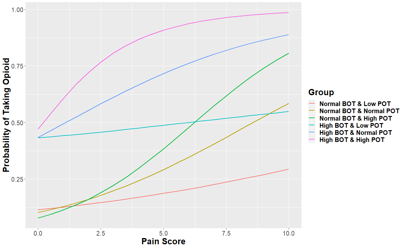
Figure 2: Estimated Probability of Taking Preoperative Opioids Against Pain Score Stratified by Risk Groups

Tables 5 and 6 show the characteristics for each subgroup. Patients in the high risk group (high BOT & normal and high BOT & high POT) and the moderate risk group (normal BOT & high POT and high BOT & low POT) tend to be more obese, younger, and have higher Fibromyalgia Survey Scores and higher Charlson Comorbidity Indices than those in the low risk group. African Americans constitute about 17% of patients in the high risk group, while there are only 5% African Americans in the low risk group. Most of patients (100% for high BOT & normal POT group and 83% for high BOT & high POT group) in the high risk group have tobacco consumption. Patients are more likely to have illicit drug use history and sleep apnea in the high and moderate risk groups than in the low risk group. A large portion of patients in the high risk group (high BOT & normal POT: 97.83%, high BOT & high POT: 66.67%) have an ASA score of 3 or above, indicating a very poor overall physical condition.

We also perform an ANCOVA-type analysis to understand the importance of each covariate’s contributions to the developed risk scores (Table 5, Table 6). Specifically, we use the log-transformed POT and BOT as response variables to fit separate linear models and calculate $R^{2}$ for each preoperative characteristic. Based on the $R^{2}$, Fibromyalgia Survey Score and ASA Score explain the most variations of BOT, while Fibromyalgia Survey Score, age and Charlson Comorbidity Index explain the most variations of POT.

Table 5: Subgroup Analysis^a

	Normal BOT Low POT (N=4,889)	Normal BOT Normal POT (N=25,581)	Normal BOT High POT (N=3,597)	High BOT Low POT (N=67)	High BOT Normal POT (N=46)	High BOT High POT (N=6)	$\mathbf{R^{2}}$ (BOT,%)	$\mathbf{R^{2}}$ (POT,%)
POT	1.13 (0.07)	1.31 (0.05)	1.54 (0.12)	1.05 (0.13)	1.27 (0.06)	1.79 (0.49)
BOT	0.14 (0.10)	0.12 (0.08)	0.09 (0.07)	0.77 (0.14)	0.78 (0.13)	0.94 (0.38)
BMI	29.63 (7.28)	29.62 (6.41)	32.18 (10.31)	33.99 (9.27)	28.95 (8.80)	36.44 (23.02)	0.91	1.29
Age	52.27 (19.17)	55.02 (14.74)	41.68 (16.48)	47.58 (10.61)	50.2 (12.97)	28.5 (6.98)	1.86	2.87
Fibromyalgia Survey Score	1.16 (3.20)	5.45 (4.62)	5.38 (4.43)	2.1 (7.47)	4.2 (9.55)	8.83 (13.72)	9.47	8.22
Satisfaction with Life	9.27 (1.45)	6.99 (2.58)	7.29 (2.75)	9.6 (1.59)	8.7 (2.84)	8.5 (2.51)	2.89	1.18
Charlson Comorbidity Index	1.13 (3.07)	1.63 (3.07)	2.77 (4.55)	3 (4.86)	2 (4.08)	6.67 (5.39)	0.06	2.75
Gender							0.60	0.08
Female	2,557 (52.30)	13,854 (54.16)	2,056 (57.16)	38 (56.72)	21 (45.65)	4 (66.67)
Male	23,32 (47.70)	11,727 (45.84)	1,541 (42.84)	29 (43.28)	25 (54.35)	2 (33.33)
Race							0.22	0.03
White	4,266 (87.26)	22,915 (89.58)	3,171 (88.16)	52 (77.61)	36 (78.26)	5 (83.33)
African American	288 (5.89)	1,263 (4.94)	208 (5.78)	12 (17.91)	8 (17.39)	1 (16.67)
Asian	95 (1.94)	327 (1.28)	44 (1.22)	1 (1.49)	0 (0.00)	0 (0.00)
Other	240 (4.91)	1,076 (4.21)	174 (4.84)	2 (2.99)	2 (4.35)	0 (0.00)
Tobacco use							16.96	0.69
No	3,217 (65.80)	14,417 (56.36)	2,064 (57.38)	4 (5.97)	0 (0.00)	1 (16.67)
Yes	1,672 (34.20)	11,164 (43.64)	1,533 (42.62)	63 (94.03)	46 (100)	5 (83.33)
Alcohol consumption							1.36	< 0.01
No	2,807 (57.41)	14,026 (54.83)	2,150 (59.77)	56 (83.58)	38 (82.61)	4 (66.67)
Yes	2,082 (42.59)	11,555 (45.17)	1,447 (40.23)	11 (16.42)	8 (17.39)	2 (33.33)
Illicit drug use							0.97	< 0.01
No	4,718 (96.50)	24,506 (95.80)	3,380 (93.97)	60 (89.55)	32 (69.57)	4 (66.67)
Yes	171 (3.50)	1,075 (4.20)	217 (6.03)	7 (10.45)	14 (30.43)	2 (33.33)
Sleep apnea							1.48	0.02
No	3,948 (80.75)	19,352 (75.65)	2,843 (79.04)	36 (53.73)	25 (54.35)	5 (83.33)
Yes	941 (19.25)	6,229 (24.35)	754 (20.96)	31 (46.27)	21 (45.65)	1 (16.67)

• mean (SD) for each continuous characteristic and frequency (percentage) for each categorical characteristic are reported.

Table 6: Subgroup Analysis^a (Continued)

	Normal BOT Low POT (N=4,889)	Normal BOT Normal POT (N=25,581)	Normal BOT High POT (N=3,597)	High BOT Low POT (N=67)	High BOT Normal POT (N=46)	High BOT High POT (N=6)	$\mathbf{R^{2}}$ (BOT,%)	$\mathbf{R^{2}}$ (POT,%)
Depression							1.50	0.29
No	4,692 (95.97)	20,444 (79.92)	3,022 (84.01)	63 (94.03)	40 (86.96)	5 (83.33)
Yes	197 (4.03)	5,137 (20.08)	575 (15.99)	4 (5.97)	6 (13.04)	1 (16.67)
Anxiety							0.79	0.20
No	4,383 (89.65)	16,567 (64.76)	2,308 (64.16)	62 (92.54)	40 (86.96)	4 (66.67)
Yes	506 (10.35)	9,014 (35.24)	1,289 (35.84)	5 (7.46)	6 (13.04)	2 (33.33)
ASA score							8.26	< 0.01
0-2	3,389 (69.32)	16,102 (62.95)	2402 (66.78)	2 (2.99)	1 (2.17)	2 (33.33)
3-4	1,500 (30.68)	9,479 (37.05)	1,195 (33.22)	65 (97.01)	45 (97.83)	4 (66.67)
Body area							2.05	2.29
Head	835 (17.08)	2,507 (9.80)	361 (10.04)	9 (13.43)	1 (2.17)	1 (16.67)
Neck	480 (9.82)	3,198 (12.5)	460 (12.79)	5 (7.46)	6 (13.04)	1 (16.67)
Thorax	286 (5.85)	1,660 (6.49)	214 (5.95)	4 (5.97)	3 (6.52)	0 (0.00)
Intrathoracic	332 (6.79)	1,095 (4.28)	120 (3.34)	5 (7.46)	1 (2.17)	0 (0.00)
Shoulder/Axilla	279 (5.71)	1,399 (5.47)	170 (4.73)	5 (7.46)	1 (2.17)	0 (0.00)
Upper Arm & Elbow	18 (0.37)	189 (0.74)	36 (1.00)	0 (0.00)	2 (4.35)	0 (0.00)
Forearm, Wrist, Hand	414 (8.47)	848 (3.31)	94 (2.61)	3 (4.48)	0 (0.00)	0 (0.00)
Upper Abdomen	325 (6.65)	2,443 (9.55)	506 (14.07)	16 (23.88)	8 (17.39)	0 (0.00)
Lower Abdomen	716 (14.65)	4,176 (16.32)	666 (18.52)	6 (8.96)	3 (6.52)	2 (33.33)
Spine/Spinal Cord	66 (1.35)	1,296 (5.07)	102 (2.84)	4 (5.97)	4 (8.70)	0 (0.00)
Perineum	416 (8.51)	2,707 (10.58)	359 (9.98)	7 (10.45)	8 (17.39)	0 (0.00)
Pelvis (Except Hip)	12 (0.25)	92 (0.36)	20 (0.56)	0 (0.00)	1 (2.17)	0 (0.00)
Upper Leg (Except Knee)	107 (2.19)	1352 (5.29)	120 (3.34)	0 (0.00)	2 (4.35)	1 (16.67)
Knee/Popliteal	424 (8.67)	1,384 (5.41)	124 (3.45)	0 (0.00)	1 (2.17)	0 (0.00)
Lower Leg	89 (1.82)	540 (2.11)	140 (3.89)	1 (1.49)	1 (2.17)	1 (16.67)
Other	90 (1.84)	695 (2.72)	105 (2.92)	2 (2.99)	4 (8.7)	0 (0.00)

• mean (SD) for each continuous characteristic and frequency (percentage) for each categorical characteristic are reported.

5.4 Discussion

The proposed INNER model achieves predictability comparable to DNN, but with more interpretability. The model leads to two metrics, BOT and POT, that may decipher the patterns of preoperative opioid use and explain the association between preoperative characteristics and preoperative opioid use. Patients with higher BMI and worse physical conditions (higher Charlson Comorbidity Indices, higher Fibromyalgia Survey Scores and higher ASA Scores) are more likely to consume preoperative opioids, and African American patients are more likely to be in the high and moderate risk groups. Patients with illicit drug use history and tobacco consumption are more likely to take preoperative opioids, while patients with alcohol consumption are less likely to have preoperative opioids. Patients with sleep apnea have a higher risk of taking preoperative opioids, as do patients expecting upper abdomen surgery. Detailed discussions of these subgroups can be found in the Appendix C.

Our results are largely consistent with the literature, which shows, for example, that patients with worse physical conditions are more likely to use preoperative opioids [Sullivan et al. (2005); Westermann et al. (2018); Goesling et al. (2015); Meredith et al. (2019)]. Prentice et al. (2019) find that high BMI and Black race are preoperative risk factors for opioid use. Younger patients are reported to have a higher risk of preoperative opioid use controlling for sociodemographics and clinical variables [Sullivan et al. (2006)]. Similarly, Lo-Ciganic et al. (2019) find that age is the among the most important features for opioid overdose prediction. Hah et al. (2015) report that patients with poor sleep quality are more likely to have preoperative opioid use. Tobacco use is reported to be a risk factor of preoperative opioid use by many studies [Westermann et al. (2018); Meredith et al. (2019)]. As for substance abuse, many studies find that subjects with drug use have higher risks of opioid use [Sullivan et al. (2006, 2005)]. Both Dong et al. (2019) and Che et al. (2017) find that substance abuse history is among the most important features for opioid dependence prediction. Sullivan et al. (2006) find that there is no significant association between problem alcohol use and opioid prescription (OR: 0.63; 95% CI: 0.35-1.15). The direction of OR in their study is consistent with our results. Sullivan et al. (2005) report a non-significant association between alcohol use and opioid prescription, though the direction is opposite from our study (OR: 1.32, P = 0.479). More studies are warranted to identify the association between alcohol consumption and preoperative opioid use.

Finally, our proposed model can be extended to accommodate generalized linear models (GLMs) as discussed in Tran et al. (2020). Specifically, let $g(\cdot)$ be a link function to link the conditional mean $\mathbb{E}(y\mid x)=g^{-1}\{\eta(x)\}$ to covariates of interest (e.g., treatment or exposure), say, $x$, where $\eta(x)=\beta_{0}+\boldsymbol{\beta}^{\top}x$. In order to model the nonlinear effects of additional features $z$ (e.g., demographics, biomarkers) on $\eta$ and achieve model flexibility, we can extend deep neural network to model the individualized intercepts and coefficients, namely, $\beta_{0}(z)$ and $\boldsymbol{\beta}(z)$. As such, the predictor can be written as $\eta(x,z)=\beta_{0}(z)+\boldsymbol{\beta}(z)^{\top}x$, which is to be linked to the conditional mean $\mathbb{E}(y\mid x,z)$ via $\mathbb{E}(y\mid x,z)=g^{-1}\{\eta(x,z)\}=g^{-1}\{\beta_{0}(z)+\boldsymbol{\beta}(z)^{\top}x\}$.

6 Conclusion

We have developed a new learning framework for robust predictions of outcomes in a more interpretable way. Beyond preoperative outcomes, we could use this approach to better predict and understand important postoperative outcomes such as opioid refill [Sekhri et al. (2018)], new chronic opioid use [Brummett et al. (2017)], hospital readmission, and opioid overdose. However, the best way to quantify the uncertainty of the estimates is still unknown. We will pursue this later.

APPENDIX

Appendix A Architecture of DNN

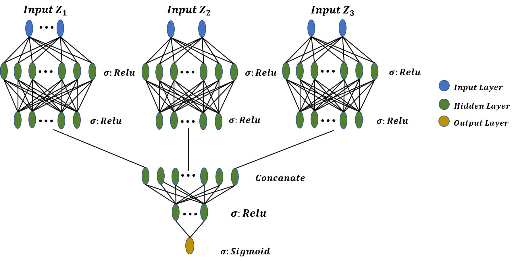
Figure A1: Architecture of DNN for the AOS Data. Input: preoperative characteristics are classified into three inputs: $Z_{1}$ are un-modifiable characteristics, such as gender and race; $Z_{2}$ are modifiable characteristics, such as BMI and smoking; $Z_{3}$ are pain-related characteristics, such as Fibromyalgia Survey Score and pain severity. Layers: each category of inputs goes through the same structure: two hidden layers with a ReLu activation function. The first hidden layer has 500 neurons and the the second hidden layer has 125 neurons. The three structures are concatenated and passed onto a layer with 15 hidden neurons and a ReLu activation function. Output: estimated probability of preoperative opioid use.

Appendix B Sensitivity Analysis

Because stochastic gradient descent is sensitive to the choice of learning rates (LR), we use grid search to tune the learning rate. For the real data analysis, we tune the learning rate over a range from 0.005 to 0.1 with 20 equally spaced grid points, and find that $LR=0.01$ seems to strike a balance between stability and computational readiness. We also implement the adaptive SGD to analyze our data. Specifically, we have implemented three popular adaptive SGD algorithms, namely, “Adagrad”, “Adadelta” and “Adam.” Adagrad adapts the learning rate based on a sequence of subgradients  [Duchi et al. (2011)] to improve the robustness of SGD and avoid tuning the learning rate manually [Dean et al. (2012)], while Adadelta [Zeiler (2012)] and Adam  [Kingma and Ba (2014)] only store an exponentially decaying average of subgradients [Zeiler (2012)]. We conduct 100 experiments to compare the prediction performance using different optimizers. In each experiment, we randomly split data into the training and testing parts, and use the balanced subsampling strategy described in Section 5.2 to assess the performance on the testing data. The means and standard errors (se) of different metrics are summarized in Table B1. We find that all four methods give similar performances, though SGD with a fixed $LR=0.01$ and Adam give the same C-statistic and sensitivity, slightly better than those obtained by Adagrad and Adadelta; all of these methods give the same balance accuracy.

Table B1: Prediction Performance of INNER Using different Optimizers^a,b

	SGD (LR=0.01)	Adagrad	Adadelta	Adam
C-statistic	0.78 (0.0006)	0.77 (0.0005)	0.76 (0.0006)	0.78 (0.0006)
Accuracy	0.72 (0.0029)	0.73 (0.0011)	0.73 (0.0006)	0.72 (0.0009)
Sensitivity	0.69 (0.0052)	0.66 (0.0022)	0.66 (0.0012)	0.69 (0.0020)
Specificity	0.73 (0.0052)	0.76 (0.0019)	0.76 (0.0010)	0.73 (0.0017)
Balance Accuracy	0.71 (0.0008)	0.71 (0.0006)	0.71 (0.0005)	0.71 (0.0006)

• used the balanced subsampling strategy and a threshold of 0.5

• based on 100 random splits

The number of iterations is chosen to ensure the convergence of the algorithm (as shown in Fig B2). We have also varied the batch sizes and number of iterations to examine the stability of the results and find a batch size of 64 and an epoch of 200 give a reasonable performance. We have conducted sensitivity analysis to assess the robustness of SGD towards the choices of these hyperparameters, and we find that the model’s C-statistic is fairly robust to them. Specifically, by varying the learning rate from 0.0075 to 0.0125, the batch size from 32 to 128 and the number of iterations from 200 to 250, the C-statistic of the obtained INNER model is around 0.78.

Table B2: Average C-statistics (se) of INNER with Various Learning Rates, Batch Sizes and Epochs^a,b,c

		LR =0.0075	LR = 0.01	LR = 0.0125
BS = 32	Epoch = 150	0.78 (0.0005)	0.78 (0.0006)	0.78 (0.0006)
	Epoch = 200	0.78 (0.0005)	0.78 (0.0007)	0.78 (0.0006)
	Epoch = 250	0.78 (0.0005)	0.78 (0.0007)	0.78 (0.0006)
BS = 64	Epoch = 150	0.78 (0.0006)	0.78 (0.0007)	0.78 (0.0007)
	Epoch = 200	0.78 (0.0005)	0.78 (0.0006)	0.78 (0.0006)
	Epoch = 250	0.78 (0.0005)	0.78 (0.0006)	0.78 (0.0005)
BS =128	Epoch = 150	0.78 (0.0006)	0.78 (0.0006)	0.78 (0.0006)
	Epoch = 200	0.78 (0.0006)	0.78 (0.0006)	0.78 (0.0006)
	Epoch = 250	0.78 (0.0006)	0.78 (0.0005)	0.78 (0.0006)

• used the balanced subsampling strategy and a threshold of 0.5

• used SGD for optimization

• based on 100 experiments

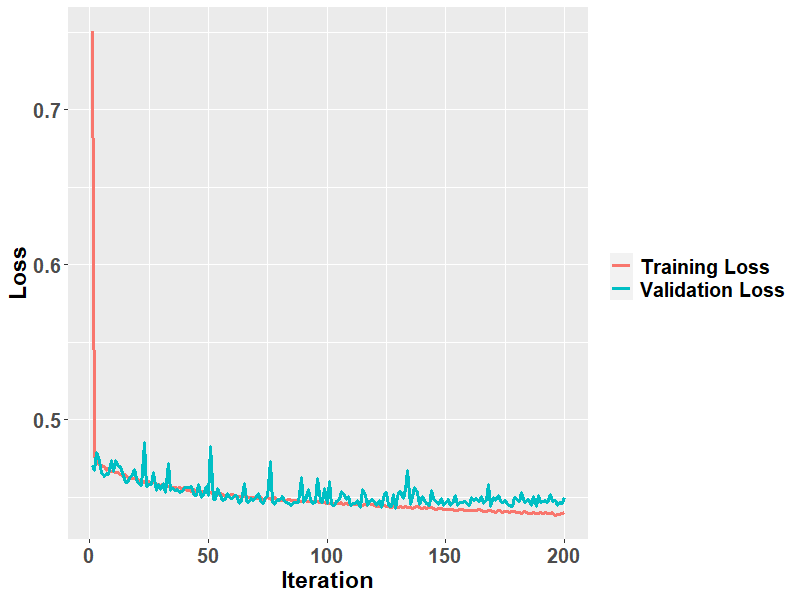
Figure B2: Learning Curve of INNER: Cross Entropy Loss Against Iteration For Training and Validation Data

We have conducted additional sensitivity analyses to examine the performance of the model under various initialization schemes for the weights $\mathbf{W}$ and the biases $\mathbf{b}$ in the neural networks. We have explored using different weights, such as uniform and normal weights, for the initial weights  [Glorot and Bengio (2010); He et al. (2015)]. In particular, we have studied two versions of uniform weights: for a weight matrix $\mathbf{W}_{l}\in\mathbf{R}^{k_{l+1}\times k_{l}}$, where $k_{l}$ and $k_{l+1}$ are the numbers of input and output units of the $l$th layer, we initialize it with $\text{Uniform}\{-\sqrt{6/(k_{l}+k_{l+1})},\sqrt{6/(k_{l}+k_{l+1)}}\}$ following Glorot and Bengio (2010) (labeled as “Glorot uniform” in Table B3, which reports the sensitivity analysis results); we also initialize the weight matrix with Uniform$(-\sqrt{6/k_{l}},\sqrt{6/k_{l}})$ following He et al. (2015) (labeled as “He uniform” in Table B3). For the normal weights, we use Normal$(0,2/(k_{l}+k_{l+1}))$ as the initial weights following Glorot and Bengio (2010) (labeled as “Glorot normal” in Table B3). Finally, for the bias vector $\mathbf{b}$, we initialize it to be either all 0’s or 1’s for its components (labeled as “Zeros” or “Ones” in the column of bias initialization in Table B3). For each set-up, we find that the C-statistic of the model is fairly constant, which is 0.78 with varied initialized values of weights and biases.

Table B3: Average (se) C-statistics with different Initializations of Weights and Biases^a,b,c

Weight Initialization	Bias Initialization	C-statistic
Glorot uniform	Zeros	0.78 (0.0006)
	Ones	0.78 (0.0006)
Glorot normal	Zeros	0.78 (0.0005)
	Ones	0.78 (0.0005)
He uniform	Zeros	0.78 (0.0008)
	Ones	0.78 (0.0006)

• used the balanced subsampling strategy and a threshold of 0.5

• used SGD for optimization

• based on 100 experiments

Table B4: Comparisons of the Prediction Performance using the AOS Data^a,b,c

	Deep Neural Network	Logistic Regression	Interpretable Neural Network Regression
Preoperative Opioid Prevalence: 0.23
C-statistic	0.78 (0.0006)	0.62 (0.0094)	0.78 (0.0006)
Threshold = 0.50
Accuracy	0.80 (0.0004)	0.70 (0.0116)	0.80 (0.0004)
Sensitivity	0.33 (0.0049)	0.43 (0.0331)	0.31 (0.0057)
Specificity	0.94 (0.0016)	0.78 (0.0238)	0.94 (0.0018)
Balance Accuracy	0.63 (0.0017)	0.61 (0.0071)	0.63 (0.002)
Threshold = 0.23
Accuracy	0.72 (0.0021)	0.69 (0.0123)	0.73 (0.0030)
Sensitivity	0.69 (0.0039)	0.44 (0.0336)	0.68 (0.0055)
Specificity	0.73 (0.0038)	0.77 (0.025)	0.74 (0.0054)
Balance Accuracy	0.71 (0.0006)	0.61 (0.007)	0.71 (0.0007)
Preoperative Opioid Prevalence: 0.50
C-statistic	0.78 (0.0006)	0.73 (0.0027)	0.78 (0.0006)
Threshold = 0.50
Accuracy	0.73 (0.0017)	0.63 (0.0129)	0.72 (0.0029)
Sensitivity	0.69 (0.0043)	0.67 (0.0261)	0.69 (0.0052)
Specificity	0.73 (0.0034)	0.62 (0.0238)	0.73 (0.0052)
Balance Accuracy	0.71 (0.0007)	0.64 (0.0049)	0.71 (0.0008)
Threshold = 0.23
Accuracy	0.46 (0.0044)	0.50 (0.0130)	0.41 (0.0056)
Sensitivity	0.93 (0.0024)	0.84 (0.0154)	0.95 (0.0022)
Specificity	0.31 (0.0064)	0.39 (0.0211)	0.24 (0.0080)
Balance Accuracy	0.62 (0.0021)	0.61 (0.0047)	0.60 (0.0030)

• prediction power of each model with the best architectures (DNN and INNER) under different sampling strategies and threshold; for the comparison of different architectures, refer to Appendix Table B5 and Appendix Table B6

• based on 100 experiments for each metric

• in the AOS data, the prevalence of preoperative opioid is 0.23, and the prevalence is around 0.23 for the training data; we use the balanced subsampling strategy to adjust the prevalence of preoperative opioid to be 0.50 in the training data

Table B5: Tuning the Architecture of INNER with the AOS Data^a,b,c,d

	Three Layers 250 Neurons	Four Layers 500 Neurons	Five Layers 500 Neurons
Preoperative Opioid Prevalence: 0.23
C-statistic	0.78 (0.0006)	0.78 (0.0007)	0.77 (0.0005)
Threshold = 0.50
Accuracy	0.80 (0.0004)	0.79 (0.0005)	0.79 (0.0004)
Sensitivity	0.31 (0.0057)	0.32 (0.0063)	0.32 (0.0061)
Specificity	0.94 (0.0018)	0.94 (0.0021)	0.93 (0.0019)
Balance Accuracy	0.63 (0.0020)	0.63 (0.0021)	0.63 (0.0021)
Threshold = 0.23
Accuracy	0.73 (0.0030)	0.72 (0.0031)	0.72 (0.0022)
Sensitivity	0.68 (0.0055)	0.68 (0.0054)	0.68 (0.0043)
Specificity	0.74 (0.0054)	0.73 (0.0055)	0.74 (0.0041)
Balance Accuracy	0.71 (0.0007)	0.71 (0.0008)	0.71 (0.0005)
Preoperative Opioid Prevalence: 0.50
C-statistic	0.78 (0.0006)	0.78 (0.0006)	0.78 (0.0006)
Threshold = 0.50
Accuracy	0.72 (0.0029)	0.73 (0.0026)	0.72 (0.0020)
Sensitivity	0.69 (0.0052)	0.69 (0.0048)	0.69 (0.0037)
Specificity	0.73 (0.0052)	0.75 (0.0047)	0.73 (0.0036)
Balance Accuracy	0.71 (0.0008)	0.71 (0.0008)	0.71 (0.0005)
Threshold = 0.23
Accuracy	0.41 (0.0056)	0.42 (0.0057)	0.43 (0.0050)
Sensitivity	0.95 (0.0022)	0.95 (0.0023)	0.94 (0.0021)
Specificity	0.24 (0.0080)	0.26 (0.0081)	0.28 (0.0071)
Balance Accuracy	0.60 (0.0030)	0.60 (0.0030)	0.61 (0.0026)

• the first column is for the best INNER architecture as reported in Table 4 and Appendix Table B4

• the other columns refer to the other more complicated INNERs, with more hidden layers or more neurons in each hidden layers

• the column names are the number of hidden layers and the number of neurons in the first hidden layers for $F_{L}(\mathbf{Z}_{i};\boldsymbol{\alpha})$ and $F_{L}(\mathbf{Z}_{i};\boldsymbol{\alpha})$

• in the AOS data, the prevalence of preoperative opioid use is 0.23; uses a balanced subsampling strategy by over-sampling cases; adjusts the prevalence of preoperative opioid use to be 0.50 in the training data

Table B6: Tuning the Architecture of DNN for AOS Data^a,b,c,d

	Two Layers 500 Neurons	Three Layer 250 Neurons	Three Layer 500 Neurons
Preoperative Opioid Prevalence: 0.23
C-statistic	0.78 (0.0006)	0.79 (0.0006)	0.79 (0.0005)
Threshold = 0.50
Accuracy	0.80 (0.0004)	0.79 (0.0004)	0.79 (0.0004)
Sensitivity	0.33 (0.0049)	0.34 (0.0054)	0.32 (0.0068)
Specificity	0.94 (0.0016)	0.93 (0.0018)	0.94 (0.0020)
Balance Accuracy	0.63 (0.0017)	0.63 (0.0018)	0.63 (0.0024)
Threshold = 0.23
Accuracy	0.72 (0.0021)	0.72 (0.0022)	0.72 (0.0024)
Sensitivity	0.69 (0.0039)	0.70 (0.0038)	0.69 (0.0049)
Specificity	0.73 (0.0038)	0.72 (0.0040)	0.73 (0.0046)
Balance Accuracy	0.71 (0.0006)	0.71 (0.0006)	0.71 (0.0005)
Preoperative Opioid Prevalence: 0.50
C-statistic	0.78 (0.0006)	0.78 (0.0006)	0.78 (0.0005)
Threshold = 0.50
Accuracy	0.73 (0.0017)	0.72 (0.0025)	0.72 (0.0023)
Sensitivity	0.69 (0.0043)	0.70 (0.0039)	0.70 (0.0043)
Specificity	0.73 (0.0034)	0.72 (0.0043)	0.73 (0.0042)
Balance Accuracy	0.71 (0.0007)	0.71 (0.0007)	0.71 (0.0005)
Threshold = 0.23
Accuracy	0.46 (0.0044)	0.45 (0.0044)	0.45 (0.0052)
Sensitivity	0.93 (0.0024)	0.94 (0.0020)	0.93 (0.0023)
Specificity	0.31 (0.0064)	0.30 (0.0062)	0.31 (0.0074)
Balance Accuracy	0.62 (0.0021)	0.62 (0.0022)	0.62 (0.0026)

• the first column is for the best DNN architecture as reported in Table 4 and Appendix Table B4

• the other columns refer to the other more complicated DNNs, with more hidden layers or more neurons

• the column names are the number of hidden layers and the number of neurons in the first hidden layers before concatenation

• in the AOS data, the prevalence of preoperative opioid use is 0.23; uses a balanced subsampling strategy by over-sampling cases; adjusts the prevalence of preoperative opioid use to be 0.50 in the training data

Appendix C Subpopulations with High Risks

We have made scatter plots of $\log(\text{POT})$ and $\log(\text{BOT})$ (Fig C3) for the three groups mentioned in Section 5.4. The population means (standard deviation (std)) of $\log(\text{POT})$ and $\log(\text{BOT})$ are 0.26 (0.09) and -2.32 (0.63) respectively. In Fig C3(a), we focus on a group of patients identified by demographic risk factors, i.e., African American male patients younger than 20 years old; these patients on average have a higher $\log(\text{POT})$ (mean: 0.29, std: 0.14) but a lower $\log(\text{BOT})$ (mean: -2.64, std: 0.46), indicating their sensitivity to pain but lower tendency to take opioids without pains. Fig C3(b) depicts BOT and POT for patients who have worsened physical conditions, i.e., with BMI greater than or equal to 32, ASA scores between three and four, Fibromyalgia survey scores greater than 13, Charlson comorbidity index greater than or equal to one, and sleep apnea; these patients have a higher $\log(\text{BOT})$ (mean: -1.33, std: 0.46) and higher $\log(\text{POT})$ (mean: 0.29, std: 0.07) compared to the entire population, indicating they are both sensitive to pain and likely to take preoperative opioids even with no pains reported. Finally, Fig C3(c) focuses on patients who have substance use and co-occurring mental disorders, such as illicit drug use history, tobacco consumption, anxiety and depression. These patients have a smaller $\log(\text{BOT})$ (mean: -1.51, std: 0.46) on average compared to those in Fig C3(b) and the highest $\log(\text{POT})$ (mean: 0.30, std: 0.07) among the three groups.

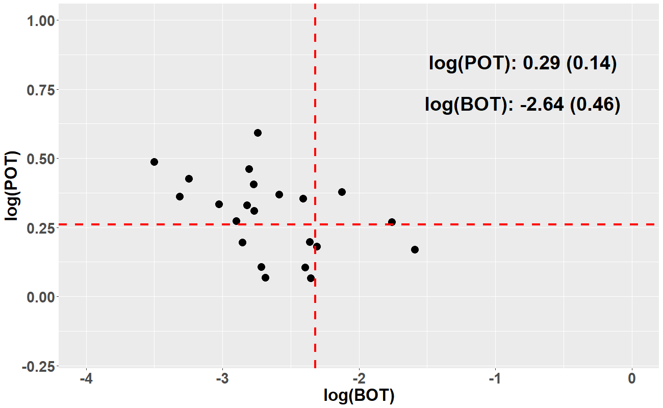
(a)

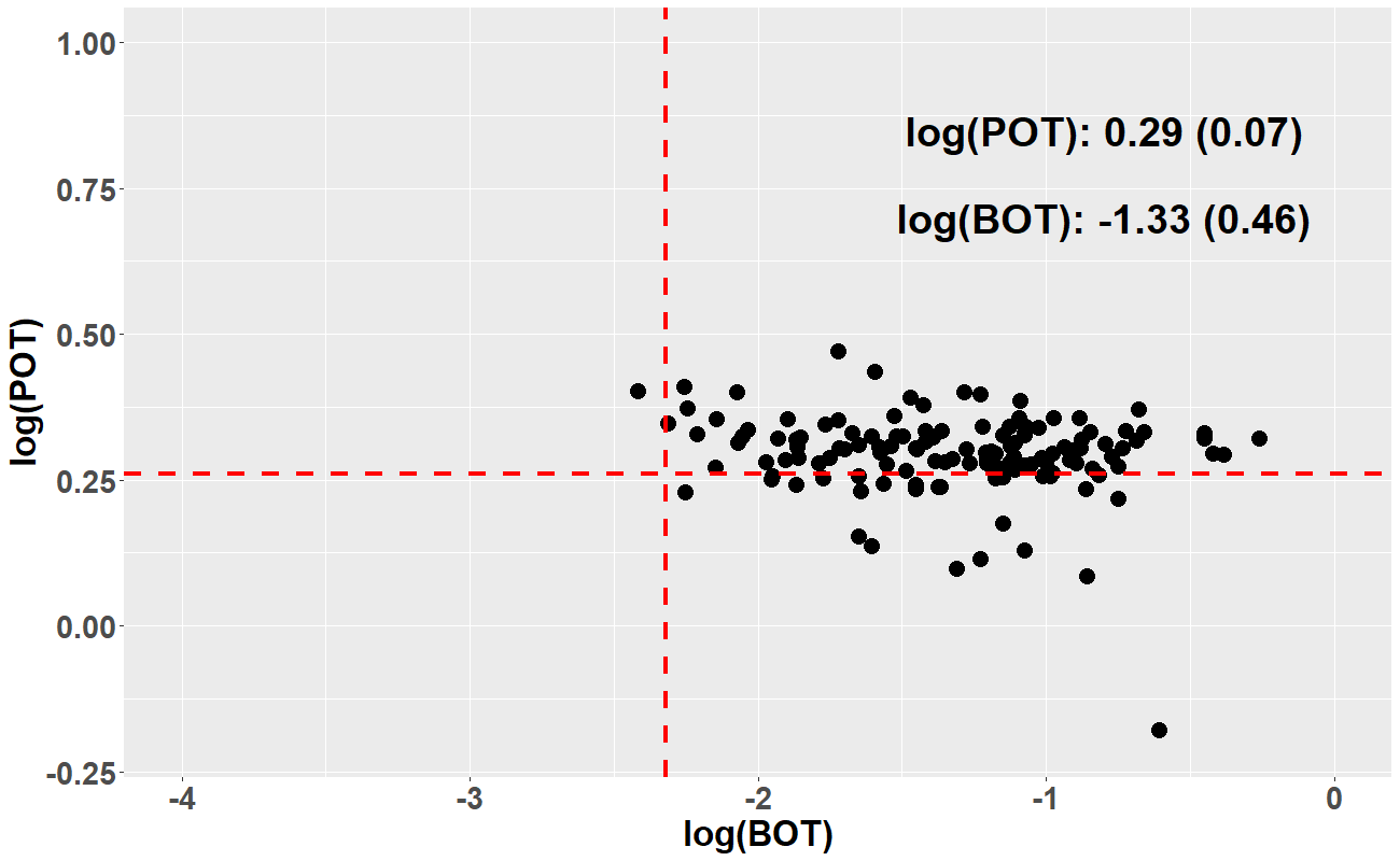
(b)

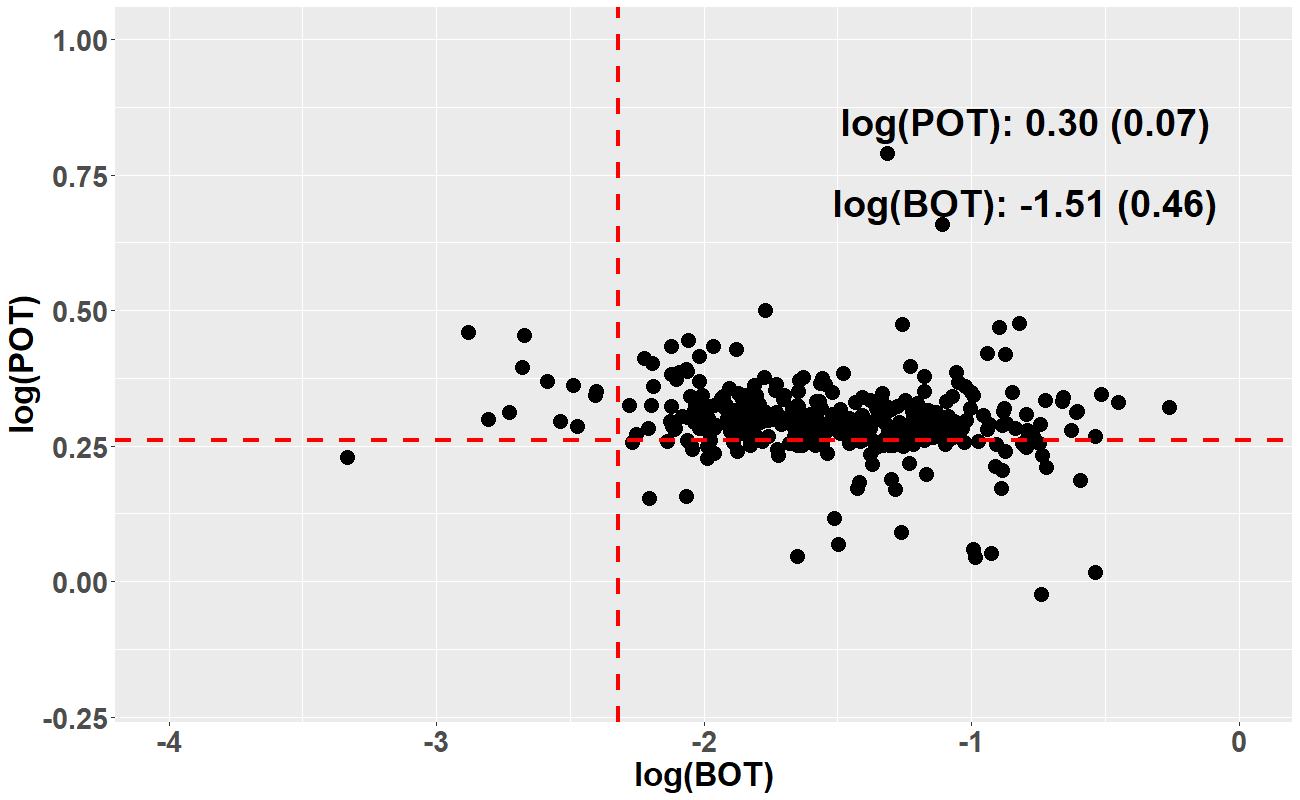
(c)

Figure C3: Distributions of BOT and POT for three groups. (a): Patients are chosen based on demographics, including gender, race and age;(b): Patients are chosen based on physical condition risk factors, including BMI, ASA scores, Fibromyalgia survey scores, Charlson comorbidity index and sleep apnea;(c): Patients are chosen based on substance use and co-occurring mental disorders, including illicit drug use history, tobacco consumption, depression and anxiety. The horizontal and vertical lines represent the population means of $\log(\text{POT})$ and $\log(\text{BOT})$, respectively; the numbers in each plot refer to the means and standard deviations.

SUPPLEMENTARY MATERIAL

Code Availability. Code developed for this project is available at https://github.com/YumingSun/INNER.

References

- Brown et al. [2021] Lily A Brown, Cecile M Denis, Anthony Leon, Michael B Blank, Steven D Douglas, Knashawn H Morales, Paul F Crits-Christoph, David S Metzger, and Dwight L Evans. Number of opioid overdoses and depression as a predictor of suicidal thoughts. Drug and Alcohol Dependence, 224:108728, 2021.
- Saha et al. [2016] Tulshi D Saha, Bradley T Kerridge, Risë B Goldstein, S Patricia Chou, Haitao Zhang, Jeesun Jung, Roger P Pickering, W June Ruan, Sharon M Smith, Boji Huang, Deborah S. Hasin, and Grant Bridget F. Nonmedical prescription opioid use and dsm-5 nonmedical prescription opioid use disorder in the United States. The Journal of Clinical Psychiatry, 77(6):772–780, 2016.
- Armaghani et al. [2014] Sheyan J Armaghani, Dennis S Lee, Jesse E Bible, Kristin R Archer, David N Shau, Harrison Kay, Chi Zhang, Matthew J McGirt, and Clinton J Devin. Preoperative opioid use and its association with perioperative opioid demand and postoperative opioid independence in patients undergoing spine surgery. Spine, 39(25):E1524–E1530, 2014.
- Schoenfeld et al. [2018] Andrew J Schoenfeld, Philip J Belmont Jr, Justin A Blucher, Wei Jiang, Muhammad Ali Chaudhary, Tracey Koehlmoos, James D Kang, and Adil H Haider. Sustained preoperative opioid use is a predictor of continued use following spine surgery. JBJS, 100(11):914–921, 2018.
- Lee et al. [2014] Dennis Lee, Sheyan Armaghani, Kristin R Archer, Jesse Bible, David Shau, Harrison Kay, Chi Zhang, Matthew J McGirt, and Clinton Devin. Preoperative opioid use as a predictor of adverse postoperative self-reported outcomes in patients undergoing spine surgery. JBJS, 96(11):e89(1)–e89(8), 2014.
- Smith et al. [2017] Savannah R Smith, Jennifer Bido, Jamie E Collins, Heidi Yang, Jeffrey N Katz, and Elena Losina. Impact of preoperative opioid use on total knee arthroplasty outcomes. The Journal of Bone and Joint Surgery, 99(10):803–808, 2017.
- Morris et al. [2016] Brent J Morris, Aaron D Sciascia, Cale A Jacobs, and T Bradley Edwards. Preoperative opioid use associated with worse outcomes after anatomic shoulder arthroplasty. Journal of Shoulder and Elbow Surgery, 25(4):619–623, 2016.
- Jain et al. [2018] Nikhil Jain, John L Brock, Frank M Phillips, Tristan Weaver, and Safdar N Khan. Chronic preoperative opioid use is a risk factor for increased complications, resource use, and costs after cervical fusion. The Spine Journal, 18(11):1989–1998, 2018.
- Cron et al. [2017] David C Cron, Michael J Englesbe, Christian J Bolton, Melvin T Joseph, Kristen L Carrier, Stephanie E Moser, Jennifer F Waljee, Paul E Hilliard, Sachin Kheterpal, and Chad M Brummett. Preoperative opioid use is independently associated with increased costs and worse outcomes after major abdominal surgery. Annals of Surgery, 265(4):695–701, 2017.
- Waljee et al. [2017] Jennifer Waljee, David Cron, Rena Steiger, Lin Zhong, Michael Englesbe, and Chad Brummett. The Effect of Preoperative Opioid Exposure on Healthcare Utilization and Expenditures Following Elective Abdominal Surgery. Annals of Surgery, 265(4):715–721, 2017.
- Hilliard et al. [2018] Paul E Hilliard, Jennifer Waljee, Stephanie Moser, Lynn Metz, Michael Mathis, Jenna Goesling, David Cron, Daniel J Clauw, Michael Englesbe, Goncalo Abecasis, and Chad M. Brummett. Prevalence of preoperative opioid use and characteristics associated with opioid use among patients presenting for surgery. JAMA Surgery, 153(10):929–937, 2018.
- Roeckel et al. [2016] Laurie-Anne Roeckel, Glenn-Marie Le Coz, Claire Gavériaux-Ruff, and Frédéric Simonin. Opioid-induced hyperalgesia: cellular and molecular mechanisms. Neuroscience, 338:160–182, 2016.
- Brummett et al. [2013] Chad M Brummett, Allison M Janda, Christa M Schueller, Alex Tsodikov, Michelle Morris, David A Williams, and Daniel J Clauw. Survey criteria for fibromyalgia independently predict increased postoperative opioid consumption after lower extremity joint arthroplasty: a prospective, observational cohort study. Anesthesiology, 119(6):1434–1443, 2013.
- Brummett et al. [2015] Chad M Brummett, Andrew G Urquhart, Afton L Hassett, Alex Tsodikov, Brian R Hallstrom, Nathan I Wood, David A Williams, and Daniel J Clauw. Characteristics of fibromyalgia independently predict poorer long-term analgesic outcomes following total knee and hip arthroplasty. Arthritis & Rheumatology, 67(5):1386–1394, 2015.
- Park et al. [2015] Byeong U Park, Enno Mammen, Young K Lee, and Eun Ryung Lee. Varying coefficient regression models: a review and new developments. International Statistical Review, 83(1):36–64, 2015.
- Hastie and Tibshirani [1993] Trevor Hastie and Robert Tibshirani. Varying-coefficient models. Journal of the Royal Statistical Society: Series B (Methodological), 55(4):757–779, 1993.
- Cai et al. [2000] Zongwu Cai, Jianqing Fan, and Runze Li. Efficient estimation and inferences for varying-coefficient models. Journal of the American Statistical Association, 95(451):888–902, 2000.
- Bauer and Kohler [2019] Benedikt Bauer and Michael Kohler. On deep learning as a remedy for the curse of dimensionality in nonparametric regression. Annals of Statistics, 47(4):2261–2285, 2019.
- Schmidt-Hieber [2020] Johannes Schmidt-Hieber. Nonparametric regression using deep neural networks with relu activation function. Annals of Statistics, 48(4):1875–1897, 2020.
- Che et al. [2015] Zhengping Che, David Kale, Wenzhe Li, Mohammad Taha Bahadori, and Yan Liu. Deep computational phenotyping. In Proceedings of the 21st ACM SIGKDD International Conference on Knowledge Discovery and Data Mining, pages 507–516. ACM, 2015.
- Lipton et al. [2015] Zachary C Lipton, David C Kale, Charles Elkan, and Randall Wetzel. Learning to diagnose with LSTM recurrent neural networks. arXiv preprint arXiv:1511.03677, 2015.
- Kleesiek et al. [2016] Jens Kleesiek, Gregor Urban, Alexander Hubert, Daniel Schwarz, Klaus Maier-Hein, Martin Bendszus, and Armin Biller. Deep mri brain extraction: a 3D convolutional neural network for skull stripping. NeuroImage, 129:460–469, 2016.
- Tran [2016] Phi Vu Tran. A fully convolutional neural network for cardiac segmentation in short-axis MRI. arXiv preprint arXiv:1604.00494, 2016.
- Choi et al. [2016] Edward Choi, Mohammad Taha Bahadori, Andy Schuetz, Walter F Stewart, and Jimeng Sun. Doctor ai: Predicting clinical events via recurrent neural networks. In Machine Learning for Healthcare Conference, pages 301–318, 2016.
- Dong et al. [2019] Xinyu Dong, Sina Rashidian, Yu Wang, Janos Hajagos, Xia Zhao, Richard N Rosenthal, Jun Kong, Mary Saltz, Joel Saltz, and Fusheng Wang. Machine learning based opioid overdose prediction using electronic health records. In AMIA Annual Symposium Proceedings, volume 2019, pages 389–398. American Medical Informatics Association, 2019.
- Lo-Ciganic et al. [2019] Wei-Hsuan Lo-Ciganic, James L Huang, Hao H Zhang, Jeremy C Weiss, Yonghui Wu, C Kent Kwoh, Julie M Donohue, Gerald Cochran, Adam J Gordon, Daniel C Malone, Courtney C. Kuza, and Walid F. Gellad. Evaluation of machine-learning algorithms for predicting opioid overdose risk among medicare beneficiaries with opioid prescriptions. JAMA Network Open, 2(3):e190968(1)–e190968(15), 2019.
- Che et al. [2017] Zhengping Che, Jennifer St Sauver, Hongfang Liu, and Yan Liu. Deep learning solutions for classifying patients on opioid use. In AMIA Annual Symposium Proceedings, volume 2017, pages 525–534. American Medical Informatics Association, 2017.
- LeCun et al. [2015] Yann LeCun, Yoshua Bengio, and Geoffrey Hinton. Deep learning. Nature, 521(7553):436–444, 2015.
- Shrestha and Mahmood [2019] Ajay Shrestha and Ausif Mahmood. Review of deep learning algorithms and architectures. IEEE Access, 7:53040–53065, 2019.
- Fan et al. [2021] Jianqing Fan, Cong Ma, and Yiqiao Zhong. A selective overview of deep learning. Statistical science: A Review Journal of the Institute of Mathematical Statistics, 36(2):264–290, 2021.
- Karlik and Olgac [2011] Bekir Karlik and A Vehbi Olgac. Performance analysis of various activation functions in generalized MLP architectures of neural networks. International Journal of Artificial Intelligence and Expert Systems, 1(4):111–122, 2011.
- Li and Yuan [2017] Yuanzhi Li and Yang Yuan. Convergence analysis of two-layer neural networks with relu activation. In Advances in Neural Information Processing Systems, pages 597–607, 2017.
- Srivastava et al. [2014] Nitish Srivastava, Geoffrey Hinton, Alex Krizhevsky, Ilya Sutskever, and Ruslan Salakhutdinov. Dropout: a simple way to prevent neural networks from overfitting. The Journal of Machine Learning Research, 15(1):1929–1958, 2014.
- Bottou [2010] Léon Bottou. Large-scale machine learning with stochastic gradient descent. In Proceedings of COMPSTAT’2010, pages 177–186. Springer, 2010.
- Liu et al. [2020] Liyuan Liu, Haoming Jiang, Pengcheng He, Weizhu Chen, Xiaodong Liu, Jianfeng Gao, and Jiawei Han. On the variance of the adaptive learning rate and beyond. In International Conference on Learning Representations, 2020. URL https://openreview.net/forum?id=rkgz2aEKDr.
- Darken et al. [1992] C. Darken, J. Chang, and J. Moody. Learning rate schedules for faster stochastic gradient search. In Neural Networks for Signal Processing II Proceedings of the 1992 IEEE Workshop, pages 3–12, 1992. doi:10.1109/NNSP.1992.253713.
- Brummett et al. [2017] Chad M Brummett, Jennifer F Waljee, Jenna Goesling, Stephanie Moser, Paul Lin, Michael J Englesbe, Amy SB Bohnert, Sachin Kheterpal, and Brahmajee K Nallamothu. New persistent opioid use after minor and major surgical procedures in US adults. JAMA Surgery, 152(6):e170504(1)–e170504(9), 2017.
- Janda et al. [2015] Allison M Janda, Sawsan As-Sanie, Baskar Rajala, Alex Tsodikov, Stephanie E Moser, Daniel J Clauw, and Chad M Brummett. Fibromyalgia survey criteria are associated with increased postoperative opioid consumption in women undergoing hysterectomy. Anesthesiology: The Journal of the American Society of Anesthesiologists, 122(5):1103–1111, 2015.
- Goesling et al. [2016] Jenna Goesling, Stephanie E Moser, Bilal Zaidi, Afton L Hassett, Paul Hilliard, Brian Hallstrom, Daniel J Clauw, and Chad M Brummett. Trends and predictors of opioid use following total knee and total hip arthroplasty. Pain, 157(6):1259–1275, 2016.
- Tan et al. [2004] Gabriel Tan, Mark P Jensen, John I Thornby, and Bilal F Shanti. Validation of the Brief Pain Inventory for chronic nonmalignant pain. The Journal of Pain, 5(2):133–137, 2004.
- Efron [2004] Bradley Efron. Large-scale simultaneous hypothesis testing: the choice of a null hypothesis. Journal of the American Statistical Association, 99(465):96–104, 2004.
- Efron [2007a] Bradley Efron. Size, power and false discovery rates. The Annals of Statistics, 35(4):1351–1377, 2007a.
- Efron [2007b] Bradley Efron. Correlation and large-scale simultaneous significance testing. Journal of the American Statistical Association, 102(477):93–103, 2007b.
- Sullivan et al. [2005] Mark D Sullivan, Mark J Edlund, Diane Steffick, and Jürgen Unützer. Regular use of prescribed opioids: association with common psychiatric disorders. Pain, 119(1-3):95–103, 2005.
- Westermann et al. [2018] Robert W Westermann, Jennifer Hu, Mia S Hagen, Michael Willey, Thomas Sean Lynch, and James Rosneck. Epidemiology and detrimental impact of opioid use in patients undergoing arthroscopic treatment of femoroacetabular impingement syndrome. Arthroscopy: The Journal of Arthroscopic & Related Surgery, 34(10):2832–2836, 2018.
- Goesling et al. [2015] Jenna Goesling, Matthew J Henry, Stephanie E Moser, Mohit Rastogi, Afton L Hassett, Daniel J Clauw, and Chad M Brummett. Symptoms of depression are associated with opioid use regardless of pain severity and physical functioning among treatment-seeking patients with chronic pain. The Journal of Pain, 16(9):844–851, 2015.
- Meredith et al. [2019] Sean J Meredith, Vidushan Nadarajah, Julio J Jauregui, Michael P Smuda, Shaun H Medina, Craig H Bennett, Jonathan D Packer, and R Frank Henn III. Preoperative opioid use in knee surgery patients. The Journal of Knee Surgery, 32(07):630–636, 2019.
- Prentice et al. [2019] Heather A Prentice, Maria CS Inacio, Anshuman Singh, Robert S Namba, and Elizabeth W Paxton. Preoperative risk factors for opioid utilization after total hip arthroplasty. JBJS, 101(18):1670–1678, 2019.
- Sullivan et al. [2006] Mark D Sullivan, Mark J Edlund, Lily Zhang, Jürgen Unützer, and Kenneth B Wells. Association between mental health disorders, problem drug use, and regular prescription opioid use. Archives of Internal Medicine, 166(19):2087–2093, 2006.
- Hah et al. [2015] Jennifer M Hah, Yasamin Sharifzadeh, Bing M Wang, Matthew J Gillespie, Stuart B Goodman, Sean C Mackey, and Ian R Carroll. Factors associated with opioid use in a cohort of patients presenting for surgery. Pain Research and Treatment, 2015, 2015.
- Tran et al. [2020] M-N Tran, Nghia Nguyen, David Nott, and Robert Kohn. Bayesian deep net glm and glmm. Journal of Computational and Graphical Statistics, 29(1):97–113, 2020.
- Sekhri et al. [2018] Shaina Sekhri, Nonie S Arora, Hannah Cottrell, Timothy Baerg, Anthony Duncan, Hsou Mei Hu, Michael J Englesbe, Chad Brummett, and Jennifer F Waljee. Probability of opioid prescription refilling after surgery: does initial prescription dose matter? Annals of Surgery, 268(2):271–276, 2018.
- Duchi et al. [2011] John Duchi, Elad Hazan, and Yoram Singer. Adaptive subgradient methods for online learning and stochastic optimization. Journal of Machine Learning Research, 12(7):2121–2159, 2011.
- Dean et al. [2012] Jeffrey Dean, Greg Corrado, Rajat Monga, Kai Chen, Matthieu Devin, Mark Mao, Marc’aurelio Ranzato, Andrew Senior, Paul Tucker, Ke Yang, and Andrew Y. Ng. Large scale distributed deep networks. Advances in Neural Information Processing Systems, 25:1223–1231, 2012.
- Zeiler [2012] Matthew D Zeiler. Adadelta: an adaptive learning rate method. arXiv preprint arXiv:1212.5701, 2012.
- Kingma and Ba [2014] Diederik P Kingma and Jimmy Ba. Adam: A method for stochastic optimization. arXiv preprint arXiv:1412.6980, 2014.
- Glorot and Bengio [2010] Xavier Glorot and Yoshua Bengio. Understanding the difficulty of training deep feedforward neural networks. In Proceedings of the Thirteenth International Conference on Artificial Intelligence and Statistics, pages 249–256. JMLR Workshop and Conference Proceedings, 2010.
- He et al. [2015] Kaiming He, Xiangyu Zhang, Shaoqing Ren, and Jian Sun. Delving deep into rectifiers: Surpassing human-level performance on imagenet classification. In Proceedings of the IEEE International Conference on Computer Vision, pages 1026–1034, 2015.