LPC-AD: Fast and Accurate Multivariate Time Series Anomaly Detection via Latent Predictive Coding

Abstract

This paper proposes LPC-AD, a fast and accurate multivariate time series (MTS) anomaly detection method. LPC-AD is motivated by the ever-increasing needs for fast and accurate MTS anomaly detection methods to support fast troubleshooting in cloud computing, micro-service systems, etc. LPC-AD is fast in the sense that its reduces the training time by as high as 38.2% compared to the state-of-the-art (SOTA) deep learning methods that focus on training speed. LPC-AD is accurate in the sense that it improves the detection accuracy by as high as 18.9% compared to SOTA sophisticated deep learning methods that focus on enhancing detection accuracy. Methodologically, LPC-AD contributes a generic architecture LPC-Reconstruct for one to attain different trade-offs between training speed and detection accuracy. More specifically, LPC-Reconstruct is built on ideas from autoencoder for reducing redundancy in time series, latent predictive coding for capturing temporal dependence in MTS, and randomized perturbation for avoiding overfitting of anomalous dependence in the training data. We present simple instantiations of LPC-Reconstruct to attain fast training speed, where we propose a simple randomized perturbation method. The superior performance of LPC-AD over SOTA methods is validated by extensive experiments on four large real-world datasets. Experiment results also show the necessity and benefit of each component of the LPC-Reconstruct architecture and that LPC-AD is robust to hyper parameters.

1 Introduction

Multivariate time series serves as an important reference of the “health status” of many Internet applications such cloud computing, micro-service systems and the Internet routing network, to name a few. For example, consider the cloud computing system, which has become a crucial infrastructure for many customized services of companies and governments [22, 26, 19]. To maintain a high quality of service of the cloud computing system, it is important to monitor the “health status” of the cloud system and perform troubleshooting in real-time [19, 22, 26]. To achieve this, many performance metrics of a cloud computing system such as CPU usage, disk I/O rate, network packet loss rate, etc., are monitored in real-time, which form a MTS [19, 22, 26]. From the MTS, system anomalies can be detected via machine learning [4, 12, 17, 23, 37, 42]. which greatly improves troubleshooting of the system.

Real-world applications like cloud computing, micro-service systems, etc., generate large amount and high dimensional time series data and they needed to be processed by fast and accurate MTS anomaly detection methods. Although many machine learning algorithms were proposed to detect anomalies in MTS [4, 12, 17, 23, 29, 37, 42], how to achieve a fast training speed while retaining fairly high detection accuracy is underexplored. Classical methods like [6, 14, 20, 29, 39, 41] have a fast training speed, but their detection accuracy is not high, due to low expressiveness capability of their model. Using deep learning models, methods like [9, 18, 28, 36] break the records of classical methods with a surprisingly high detection accuracy thanks to high expressiveness of these models. In the research line of modern methods, most efforts were spent on developing sophisticated models to improve detection accuracy [9, 18, 28, 36]. As a consequence, these sophisticated models becomes more and more time-consuming for training. Recently, the USAD [4] and TranAD [37] improve the training speed, while retaining a fairly high accuracy. These two algorithms follow the same architecture of adversarial training (refer to Section 2 for details) and their detection accuracy can be low in some datasets (refer to Section 6 for details). This paper aims to explore faster training speed and more accurate MTS anomaly detection methods.

It is challenging to design fast and accurate MTS anomaly detection algorithms. First, the MTS training data is usually not associated with anomalous labels and there is no specification on the pattern of an anomaly in general [4, 37]. Second, the anomalous data points in MTS training data can mislead the trained model [18]. Third, the MTS data is usually of high dimension and it has complex spatial and temporal dependence [4, 37], where the spatial dependence refers to the dependence among different time series. This makes it difficult to learn the normal and abnormal pattern from the MTS. Fourth, the MTS data is usually non-stationary, [19] making it difficult to learn stable patterns. In this paper, we propose an algorithm called LPC-AD to address these challenges.

The LPC-AD has a shorter training time than SOTA deep learning methods that focus on reducing training time, and it has a higher detection accuracy than SOTA sophisticated deep learning based methods that focus on enhancing detection accuracy. These merits of LPC-AD are supported by novelty in the design and extensive empirical evaluation on four large real-world datasets.

Novelty in the design. Though the LPC-AD falls into the research line of autoencoder based methods [4, 17, 37, 42, 12] that learn the normal spatial and temporal dependence in the MTS data to detect anomaly (refer to Section 2 for details on this research line), it contributes several new ideas. Unlike previous works [4, 17, 37, 42, 12] which use autoencoder to capture spatial and temporal dependence in many MTS, we use autoencoder to reduce redundancy in the time series data. Through this we obtain a low dimensional latent representation of the data. Evidence of redundancy in MTS can be found in [19, 22, 26]. As our purpose is to reduce redundancy, simple autoencoders such as vanilla LSTM based autoencoder suffice. To capture temporal dependence in MTS, we apply ideas from predictive coding [3], which have been successfully applied to word representation[27], image colorization[43], and visual representation learning [11], etc. Note that we are the first to explore predictive coding for MTS anomaly detection. More specifically, we use a predictor to capture temporal dependence between two consecutive sliding windows of the MTS. The predictor aims to learn the normal dependence via predicting future latent variables from its preceding latent variables in the sliding window. Here, we do not need sophisticated prediction networks, as they may overfit the anomalous patterns in the training data. We then use randomized perturbation to inject some noise on the output of the predictor. Finally, we use the decoder to decode this perturbed prediction and use the absolute error between the decoded data and the ground truth time series data to measure the anomalous score of a data point. The purpose of this perturbation is to avoid overfitting to the patterns of anomaly data points, as the decoder aims to learn the normal patterns. This randomized perturbation approach has a theoretical foundation in online learning in the presence of adversarial data [1]. As an analogy, the anomalous data points in the time series are equivalent to the adversarial data in online learning. Note that this randomized perturbation only incurs a negligible computational cost. Combining them all, we contribute a generic architecture called LPC-Reconstruct in the sense that one can select different instances of the above mentioned autoencoder network, the predictor network and the randomized perturbation method to attain different tradeoffs between the training speed and detection accuracy.

To illustrate, Figure 1 visualizes anomalies detected by LPC-AD-SA in the SMD dataset, where the LPC-AD-SA denotes an instance of LPC-AD (refer to Section 6 for more details). Only two dimensions of the time series are shown for simplicity. In Figure 1, the red curve corresponds to reconstructions by LPC-AD-SA. The anomaly score is quantified by the absolute reconstruction error. The red windows correspond to the anomalous windows labeled in the dataset. The yellow windows correspond to anomalous windows detected by LPC-AD-SA. From Figure 1, one can observe that LPC-AD-SA identifies all anomalous windows out. The time series is well fitted by the reconstructions outside the anomalous windows, and is poorly fitted inside the anomalous windows.

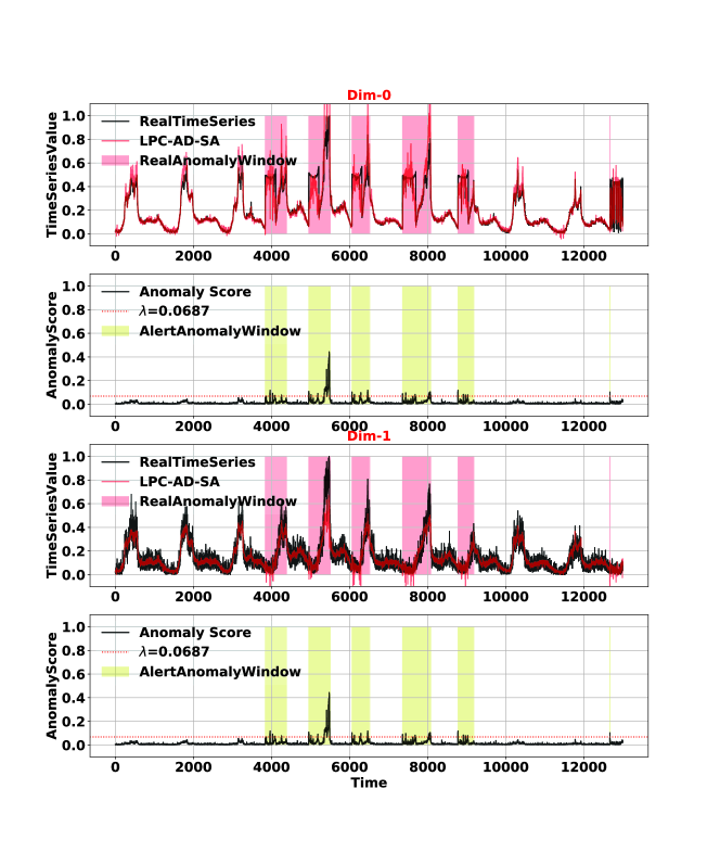
Figure 1: Visualizing the anomalies detected by LPC-AD-SA.

Extensive empirical validation. We instantiate LPC-Reconstruct with the vanilla LSTM autoencoder, three simple predictors (i.e., linear predictor, LSTM enabled predictor and attention enabled predictor) and propose a simple randomized perturbation method based on Gaussian noise. We conduct extensive experiments on four public datasets that are widely used for evaluating MTS anomaly detection algorithms. Experiment findings are summarized into four folds. First, the LPC-AD reduces the training time of SOTA deep learning methods that focus on fast training by as high as 38.2%. It improves the detection accuracy of SOTA sophisticated deep learning based methods that focus on high accuracy by as high as 18.9%. Second, LPC-AD has a high sample efficiency, i.e., reducing the training data points by 75%, its detection accuracy only drops by less than 2%. Third, LPC-AD is robust to its hyper parameters in terms of accuracy, i.e., the variation of detection accuracy is at most three percents when the hyper parameters varies in a fairly large range. Fourth, ablation study shows the necessity of each component and the benefit of each component. The highlights of our contributions include:

• A generic architecture LPC-Reconstruct, which is a novel combination of ideas from autoencoder, predictive coding and randomized perturbation.

• A simple instantiation of LPC-Reconstruct, which contributes a new randomized perturbation method to avoid overfitting of anomalous dependence patterns.

• Extensive empirical evaluations to justify superior performance and reveal fundamental understating of our method.

2 Related works

MTS anomaly detection is a challenging problem, and it has been studied extensively. From a methodological perspective, previous works can be categorized into two research lines, i.e., (1) classical methods and (2) deep learning based methods. Notable classical methods include [6, 14, 20, 29, 39, 41], just to name a few. One limitation of classical methods is that the expressiveness is low, resulting low anomaly detection accuracy [40]. Deep learning based methods address this limitation. Our work falls into the research line of deep learning based methods. Methodologically, previous works on deep learning based MTS anomaly detection methods can be categorized into four groups: (1) forecasting based methods, (2) reconstruction based methods, (3) hybrid methods combining forecasting and reconstruction , and (4) miscellaneous methods.

Forecasting based MTS anomaly detection methods [7, 8, 10, 13, 34] use a prediction function to capture normal spatial and temporal dependence in MTS, and they identify abnormal dependence, i.e., report anomaly, when the prediction error is relatively large. The LSTM-AD [34] uses a stacked LSTM to predict future data points from historical data points. It uses the likelihood of the prediction error to quantify the anomaly score of a data point, and it reports an anomaly whenever the anomaly score exceeds a given alert threshold. Chauhan et al. applied the LSTM-AD to detect anomalies in electrocardiography time series [8]. Bontemps et al. [7] used the vanilla LSTM for forecasting and quantified the anomaly score via the prediction errors of several steps. LSTM-NDT[13] also uses the vanilla LSTM for forecasting and uses the prediction error of a data point to quantify the anomaly score. It develops a non-parameterized method to select the alert threshold. However, the detection accuracy of these LSTM based MTS anomaly detection methods [7, 8, 34, 13] is not high enough, because LSTM alone lacks expressiveness to capture complex dependence in MTS [37]. Deng et al. [10] proposed a graph neural network to capture spatial dependence of multi-time series explicitly and used a graph attention network to predict future data points from historical data points. However, the graph attention network makes this method unable to capture long-term dependence well. These forecasting based methods have a relatively fast training speed, but their detection accuracy is greatly outperformed by reconstruction based methods [18, 36, 37].

Reconstruction based methods capture the normal spatial and temporal dependence in multi-time series via a low dimensional latent representation, and they identify abnormal dependence, i.e., report anomaly, when the reconstruction from the low dimensional latent representation differs from the actual observation. From a model architecture’s perspective, previous works can be categorized into autoencoder based ones [4, 17, 23, 37, 42, 12] and variational autoencoder based ones [9, 18, 28, 36, 40].

• Autoencoder (AE) based methods. The EncDec-AD [23] instantiates the autoencoder architecture with the vanilla LSTM for MTS anomaly detection. The reconstruction error of a data point quantifies the anomaly score, and EncDec-AD reports an anomaly whenever the anomaly score exceeds a given threshold. The MSCRED [42] improves the expressiveness of EncDec-AD. It uses a convolutional network to capture spatial dependence and a convolutional LSTM to capture temporal dependence. However, it is time-consuming to train the model, and it requires a large amount of training data to fit the model well. Recent autoencoder based methods [4, 17, 37] contribute simple models with a fast training speed, while retaining a fairly high detection accuracy. The openGauss [17] instantiates the autoencoder architecture with a tree-based LSTM for MTS anomaly detection. It has a fast training speed and low memory requirement. USAD [4] further improves the training speed via adversarial training. It has one simple encoder and two decoders. Two decoders share the same encoder, and the purpose of two decoders is to enable adversarial training, which amplifies the temporal anomaly. The encoder and two decoders are composed of several linear layers, enabling a fast training speed. However, simple linear layers cannot capture temporal dependence well because they can not process longer input. TranAD [37] replaced the linear layer of USAD with transformer[38] network to capture temporal dependence better. TranAD contributes a slightly more sophisticated model than USAD. It is shown to have a higher detection accuracy than USAD, while retaining a fast training speed. Compared to these works, our work presents a new architecture, which combines autoencoder, predictive coding and randomized perturbation. Furthermore, our work outperforms them in both training speed and detection accuracy.

• Variational autoencoder (VAE) based methods.: The Donut [40] extends the vanilla VAE by changing the linear layers to represent the variance of latent variables to a layer with the soft plus operation. The LSTM-VAE [28] instantiates the VAE architecture by replacing the feed-forward network of VAE with a vanilla LSTM network to capture the temporal dependence in MTS. To improve the expressiveness of Donut and LSTM-VAE, OmniAnomaly [36] changes the latent variables’ distribution of LSTM-VAE from standard Gaussian distribution to a more sophisticated distribution. The sophisticated distribution in OmniAnomaly is a combination of a linear Gaussian state space model [15] and a normalizing flow [33]. OmniAnomaly further uses latent variable linking to enhance the temporal dependence between latent variables. InterFusion [18] improves OmniAnomaly by using an anomaly pre-filtering algorithm to filter out potential anomalous data in the training set. It also compresses the multi-time series via two-view embedding. To better capture spatial dependence in MTS, the SDFVAE [9] instantiates the VAE architecture with a convolutional neural network, a BiLSTM, and recurrent VAE. Although OmniAnomaly, InterFusion and SDFVAE have high expressiveness because of their sophisticated models, their training processes are very resource-intensive and time-consuming. Different from them, our work is an autoencoder based method, and it outperforms them in both training speed and detection accuracy.

Hybrid methods combine forecasting-based methods and reconstruction based methods in the sense that they jointly optimize a forecasting model and a reconstruction model. They attempt to overcome the shortcomings that forecasting based methods and reconstruction based methods suffer on their own [35]. One notable architecture of hybrid methods is proposed by Srivastava et al. [35] This architecture contains one encoder and two decoders sharing the same encoder. One of the decoders is designed for forecasting purposes, and the other is designed for reconstruction purposes. In the seminal work on this architecture, Srivastava et al. [35] instantiated this architecture with the vanilla LSTM. Medel et al. [25] instantiated this architecture with convolutional LSTM to have a high expressiveness capability. Zhao et al. [45] instantiated this architecture with a 3D convolutional neural network for better detection of video series anomalies. These methods are mainly designed for video series, and they do not capture the spatial and temporal dependence in multi-time series well. The MTAD-GAT [44] is composed of a graph attention network for forecasting, which captures the spatial dependence, and a vanilla VAE for reconstruction, which captures the likelihood of a data point. It jointly optimizes those two models and quantifies the anomaly score with both the prediction error and the reconstruction error for anomaly detection. The CAEM [44] is composed of a convolutional autoencoder for reconstruction and a BiLSTM for forecasting. It also jointly optimizes those two models and quantifies the anomaly score with both the prediction error and the reconstruction error for anomaly detection. However, these methods have a high computational cost in training and low scalability for high-dimensional datasets. They are outperformed by autencoder based methods like TranAD [37].

Miscellaneous methods refer to notable related works that do not fall into the above research lines. The DAGMM [46] is composed of a simple autoencoder model for dimensionality reduction and a Gaussian Mixture Model [32] for density estimation. The density estimated by the GMM is used to predict the next data point. However, it is computationally expensive for training and unable to capture the spatial-temporal dependence well. Ren et al. [31] proposed estimators for the implicit likelihoods of GANs, and they showed that such estimators could be applied to detect anomalies in multi-time series data. The MAD-GAN [16] instantiated the vanilla GAN architecture with LSTM-RNN. Koopman operator is a classical method in control theory [21]. It has a similar idea of latent predictive coding. Theoretically, in an infinite-dimensional latent state space, the next state can be a linear function of the states in a recent time window [21]. In particular, when we instantiate the predictor in our LPC-AD architecture as a linear function, we get a deep Koopman operator [21]. For practical applications where we cannot have finite-dimensional states, non-linear predictor function is needed for state transitions in latent space. This is validated by our experiment in Figure 11, where we observe that using non-linear predictor functions improves the accuracy of anomaly detection.

Last, in terms of design objective, our work is closely related to USAD [4] and TranAD [37]. To the best of our knowledge, USAD and TranAD are the only two works that aim to reduce training time while retaining a fairly high detection accuracy. We proposed a generic architecture and show that simple instantiations of this architecture can outperform USAD and TranAD in training speed and outperform SOAT methods (including sophisticated models) in detection accuracy. The design of our architecture reveals new insights in exploring latent predictive coding and randomized perturbation for MTS anomaly detection.

3 Problem Formulation

We consider an $M\in\mathbb{N}_{+}$ dimensional time series indexed by time stamps $t\in\mathbb{N}_{+}$. Let $\bm{x}_{t}\triangleq(x_{t,1},\ldots,x_{t,M})\in\mathbb{R}^{M}$ denote the $t$-th observation or sample point of the time series. For example, $\bm{x}_{t}$ can be the values of $M$ KPIs of a cloud computing system measured at time stamp $t$. Note that in practice, the observations of a time series are sampled at a fixed rate or time varying rate. In this paper, we do not make any assumptions about the sampling rate. We consider the setting that we are given a training dataset of $T\in\mathbb{N}_{+}$ data points of the time series denoted by $\mathcal{T}=\{\bm{x}_{1},\ldots,\bm{x}_{T}\}$. Each data point is not associated with a label on whether it is anomalous or not. Our objective is to design and train an anomaly detection algorithm from the training dataset $\mathcal{T}$.

To make our model more robust, we normalize the time series data as follows:

$$x_{t,m}\leftarrow\frac{x_{t,m}-\min_{\tau\in\{1,\ldots,T\}}x_{\tau,m}}{\max_{\tau\in\{1,\ldots,T\}}x_{\tau,m}-\min_{\tau\in\{1,\ldots,T\}}x_{\tau,m}+\alpha},\quad\forall t,m,$$ (1)

where $\alpha\in\mathbb{R}_{+}$ denotes a smoothing factor. The smoothing factor $\alpha$ is a small positive constant vector, which prevents zero-division.

4 The LPC-AD Algorithm

Our algorithm is built on two sliding windows, i.e., a sliding window of historical data points and a sliding window of future data points. It utilizes the dependence between data points in these two sliding windows to detect the anomaly. Formally, denote a sliding window of $\ell_{h}\in\mathbb{N}_{+}$ latest historical data points up to time stamp $t$ as

$${\bm{W}}^{h}_{t}\triangleq[{\bm{x}}_{t-\ell_{h}+1},\cdots,{\bm{x}}_{t}],$$ (2)

where $t\geq\ell_{h}$. Denote a sliding window of $\ell\in\mathbb{N}_{+}$ future data points starting from time stamp $t+1$ as

$$\bm{W}_{t+1}=[\bm{x}_{t+1},\ldots,\bm{x}_{t+\ell}].$$ (3)

The window size $\ell_{h}$ and $\ell$ are two hyperparameters, and in general, they may be different, i.e., $\ell_{h}\neq\ell$. We aim to design and train an algorithm to learn the dependence between two consecutive windows, i.e., ${\bm{W}}^{h}_{t}$ and $\bm{W}_{t+1}$, from $\mathcal{T}$. And then, we utilize it to decide whether a data point $\bm{x}_{t}$ outside the training dataset, where $t>T$, is an anomaly or not.

Formally, we design an anomaly detection algorithm based on the latent predictive coding. Algorithm 1 outlines our LPC-AD (Latent Predictive Coding for Anomaly Detection) algorithm. The LPC-AD takes two consecutive sliding windows, i.e., ${\bm{W}}^{h}_{t}$ and ${\bm{W}}_{t+1}$, and an alert threshold $\lambda\in\mathbb{R}_{+}$ as input. Note that the sliding window ${\bm{W}}_{t+1}$ is outside the training dataset, i.e., $t\geq T$. It outputs an $\ell$-dimensional binary vector to indicate where a data point in the window ${\bm{W}}_{t+1}$ is anomalous or not, In Step 3 to 5, an anomaly score for each data point in ${\bm{W}}_{t+1}$ is computed, which quantifies the likelihood for a data point to be an anomaly. More specifically, the anomaly score is built on two two key ideas. The one is to utilize latent predictive coding to capture the normal dependence between two consecutive sliding windows. This is achieved by the $\texttt{LPC-Reconstruct}(\bm{W}^{h}_{t},\bm{W}_{t+1},\bm{\epsilon};\bm{\Theta})$ algorithm in Step 4. The details of LPC-Reconstruct are deferred to Section 5. The other idea is random perturbation, which is achieved by generating a stochastic noise in Step 3 and taking it as an input to the LPC-Reconstruct algorithm in Step 4. The purpose of this random perturbation is to avoid overfitting the patterns of anomaly data points. Based on the anomaly score, in the remaining steps, we use the alert threshold $\lambda$ to report the anomaly. In particular, when the anomaly score exceeds the alert threshold $\lambda$, we report an anomaly; otherwise, we report no anomaly.

Algorithm 1 LPC-AD Algorithm

1:$({\bm{W}}^{h}_{t},{\bm{W}}_{t+1}),\forall t\geq T$, alert threshold $\lambda$

2:$\bm{a}\triangleq(a_{1},\ldots,a_{\ell})$

3:$\bm{\epsilon}\sim\mathcal{N}(\bm{0},\bm{\Sigma})$

4:$[\widetilde{\bm{x}}_{t+1},\ldots,\widetilde{\bm{x}}_{t+\ell}]\leftarrow\texttt{LPC-Reconstruct}(\bm{W}^{h}_{t},\bm{W}_{t+1},\bm{\epsilon};\bm{\Theta})$

5:$\text{AnomalyScore}_{i}\leftarrow\|\bm{x}_{t+i}-\widetilde{\bm{x}}_{t+i}\|_{2},\forall i=1,\ldots,\ell$

6:$a_{i}\leftarrow\mathbb{I}_{\{\text{AnomalyScore}_{i}\geq\lambda\}},\forall i=1,\ldots,\ell$.

7:Return $\bm{a}$.

Remark 1: selection of $\lambda$. Using an alert threshold to report anomaly is widely used in previous works [4, 37, 18, 32, 36]. Though few adaptive methods were proposed to select the alert threshold automatically, these methods turned out to be either not stable or computationally expensive. As a consequence, exhaustive search method is the most widely adopted method [4, 37, 18, 32, 36]. The exhaustive search method only requires proper discretization of the domain of the alert threshold. The domain of the alert threshold depends on the underlying anomaly score evaluation method, which can be quite different across different methods [4, 37, 18, 32, 36].

Remark 2: multiple windows. When there are multiple sliding window pairs to detect, i.e., $\{({\bm{W}}^{h}_{t_{i}},{\bm{W}}_{t_{i}+1}):i=1,\ldots,I\}$, where $I\in\mathbb{N}_{+}$, one can apply Algorithm 1 to each pair of them sequentially or in parallel.

5 Design and Training of LPC-Reconstruct

In this section, we first present the general architecture of the $\texttt{LPC-Reconstruct}(\bm{W}^{h}_{t},\bm{W}_{t+1},\bm{\epsilon};\bm{\Theta})$ algorithm. Then, we present a simple instantiation of the general architecture to demonstrate the power of the proposed architecture. Lastly, we design an algorithm to train this instantiation from the training dataset $\mathcal{T}$.

5.1 General Model Architecture

We parameterize $\texttt{LPC-Reconstruct}(\bm{W}^{h}_{t},\bm{W}_{t+1},\bm{\epsilon};\bm{\Theta})$ via a neural network as shown in Figure 2. Four building blocks of this architecture are: a sequence encoder $\texttt{SeqEnc}(\cdot;\bm{\Theta}_{\text{SE}})$ with parameter $\bm{\Theta}_{\text{SE}}$, a sequence decoder $\texttt{SeqDec}(\cdot;\bm{\Theta}_{\text{SD}})$ with parameter $\bm{\Theta}_{\text{SD}}$, a predictor $\texttt{Predic}(\cdot;\bm{\Theta}_{\text{PD}})$ with parameter $\bm{\Theta}_{\text{PD}}$ and a randomized data perturbation operator $\texttt{RandPerturb}(\cdot;\bm{\Theta}_{\text{RP}})$ with parameter $\bm{\Theta}_{\text{RP}}$. We defer the design details of each of these building blocks to Section 5.2, and let us state some properties of them first, which are helpful for us to deliver the key ideas of our model architecture.

• $\texttt{SeqEnc}(\cdot;\bm{\Theta}_{\text{SE}})$. It takes a consecutive sequence of data points $\bm{x}_{t_{1}},\bm{x}_{t_{1}+1},\ldots,\bm{x}_{t_{2}}$ as the input, where $t_{1},t_{2}\in\{1,\ldots,T\}$ and $t_{1}\leq t_{2}$, and outputs an encoded low dimensional data sequence denoted by $\bm{z}_{t_{1}},\bm{z}_{t_{1}+1},\ldots,\bm{z}_{t_{2}}$, where $\bm{z}_{t}\in\mathbb{R}^{N}$, $t\in\{t_{1},\ldots,t_{2}\}$, $N\in\mathbb{N}_{+}$ and $N<M$. We call $\bm{z}_{t}$ the latent variable and it is a compression of the original data $\bm{x}_{t}$.

• $\texttt{SeqDec}(\cdot;\bm{\Theta}_{\text{SD}})$. It takes a low dimensional latent variable sequence $\bm{z}_{t_{1}},\ldots,\bm{z}_{t_{2}}$ as the input, and outputs a high dimensional decoded sequence denoted by $\widehat{\bm{x}}_{t_{1}},\ldots,\widehat{\bm{x}}_{t_{2}}$, where $\widehat{\bm{x}}_{t}\in\mathbb{R}^{M}$, $t\in\{t_{1},\ldots,t_{2}\}$. The $\widehat{\bm{x}}_{t}$ is a reconstruction of the original data $\bm{x}_{t}$.

• $\texttt{Predic}(\cdot;\bm{\Theta}_{\text{PD}})$. It takes a consecutive sequence of $\ell_{h}$ latent variables $\bm{z}_{t-\ell_{t}+1},\ldots,\bm{z}_{t}$ as the input, and outputs a prediction on the next $\ell$ latent variables $\bm{z}_{t+1},\ldots,\bm{z}_{t+\ell}$.

• $\texttt{RandPerturb}(\cdot,\bm{\epsilon};\bm{\Theta}_{\text{RP}})$. It takes the latent variable sequence predicted by $\texttt{Predic}(\cdot;\bm{\Theta}_{\text{PD}})$ and the ground truth latent variable sequence as the input, and generates a zero mean stochastic noise vector $\bm{\epsilon}$ to perturb the predictions.

In LPC-Reconstruct, we first input the data points of two consecutive sliding window, i.e., ${\bm{W}}^{h}_{t},{\bm{W}}_{t+1}$, into the encoder to obtain a low dimensional representation ${\bm{Z}}^{h}_{t},{\bm{Z}}_{t+1}$, where

$$[{\bm{Z}}^{h}_{t},{\bm{Z}}_{t+1}]=\texttt{SeqEnc}({\bm{W}}^{h}_{t},{\bm{W}}_{t+1};\bm{\Theta}_{\text{SE}}),$$

and ${\bm{Z}}^{h}_{t}=[{\bm{z}}_{t-\ell_{h}1+1},\cdots,{\bm{z}}_{t}]$ and ${\bm{Z}}^{2}_{t}=[{\bm{z}}_{t+1},\cdots,{\bm{z}}_{t+\ell}]$. The purpose of this low dimensional representation is to eliminate the redundancy in the time series data. Then we use the decoder to reconstruct the original time series from the encoded low dimensional data, i.e., ${\bm{Z}}^{h}_{t}$ and ${\bm{Z}}_{t+1}$,

$$[\widehat{\bm{W}}^{h}_{t},\widehat{\bm{W}}_{t+1}]=\texttt{SeqDec}({\bm{Z}}^{h}_{t},{\bm{Z}}_{t+1};\bm{\Theta}_{\text{SD}}),$$

where $\widehat{\bm{W}}^{h}_{t}=[\widehat{\bm{x}}_{t-\ell_{h}+1},\cdots,\widehat{\bm{x}}_{t}]$ and $\widehat{\bm{W}}_{t+1}=[\widehat{\bm{x}}_{t+1},\cdots,\widehat{\bm{x}}_{t+\ell}]$. To capture the dependence in the low dimensional representation, we use a prediction operator, which use the encoded data of the historical window to predict the data associated with the future window, formally

$$\widehat{{\bm{Z}}}_{t+1}=\texttt{Predic}({\bm{Z}}^{h}_{t};\bm{\Theta}_{\text{PD}}).$$

Then we use a randomized perturbation operator to perturb the above prediction.

$$\widetilde{\bm{Z}}_{t+1}=\texttt{RandPerturb}({\bm{Z}}_{t+1},\widehat{{\bm{Z}}}_{t+1},\bm{\epsilon};\bm{\Theta}_{\text{RP}}),$$

where $\widetilde{\bm{Z}}_{t+1}=[\widetilde{\bm{z}}_{t+1},\cdots,\widetilde{\bm{z}}_{t+\ell}]$ and $\bm{\epsilon}$ denotes an $\ell$-dimensional zero mean stochastic noise. The purpose of this perturbation is to avoid overfitting the patterns of anomaly data points, as there may be some anomaly data points in the training data. This operation also makes $\widetilde{\bm{Z}}_{t+1}$ more robust to small outliers in training data. It has a theoretical foundation in online learning in the presence of adversarial data [1]. Finally, we obtain the reconstructed data as:

$$[\widetilde{\bm{W}}^{h}_{t},\widetilde{\bm{W}}_{t+1}]=\texttt{SeqDec}({\bm{Z}}^{h}_{t},\widetilde{\bm{Z}}_{t+1};\bm{\Theta}_{\text{SD}}),$$

where $\widetilde{\bm{W}}_{t+1}$ serves as the output of $\texttt{LPC-Reconstruct}(\bm{W}^{h}_{t},\bm{W}_{t+1},\bm{\epsilon};\bm{\Theta}):$

$$\texttt{LPC-Reconstruct}(\bm{W}^{h}_{t},\bm{W}_{t+1},\bm{\epsilon};\bm{\Theta})=\widetilde{\bm{W}}_{t+1}.$$

Then, the parameter $\bm{\Theta}$ of $\texttt{LPC-Reconstruct}(\bm{W}^{h}_{t},\bm{W}_{t+1},\bm{\epsilon};\bm{\Theta})$ can be summarized as:

$$\bm{\Theta}=[\bm{\Theta}_{\text{SE}},\bm{\Theta}_{\text{SD}},\bm{\Theta}_{\text{PD}},\bm{\Theta}_{\text{RP}}].$$

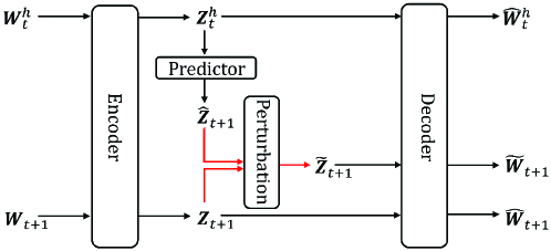
Figure 2: Architecture of $\texttt{LPC-Reconstruct}(\bm{W}^{h}_{t},\bm{W}_{t+1},\bm{\epsilon};\bm{\Theta})$.

To learn the function $\texttt{LPC-Reconstruct}(\bm{W}^{h}_{t},\bm{W}_{t+1},\bm{\epsilon};\bm{\Theta})$ from the training data $\mathcal{T}$, we consider a loss function associated with time stamp $t$ defined as:

$$L_{t}(\bm{\Theta})=\underbrace{\|{\bm{W}}^{h}_{t}-{\widehat{\bm{W}}}^{h}_{t}\|_{2}+\|{\bm{W}}_{t+1}-{\widehat{\bm{W}}}_{t+1}\|_{2}}_{\text{redundancy reduction loss}}+\underbrace{\mathbb{E}_{\bm{\epsilon}}[\|\bm{W}_{t+1}-\widetilde{\bm{W}}_{t+1}\|_{2}]}_{\text{dependency capturing loss}},$$

where the expectation notation $\mathbb{E}_{\bm{\epsilon}}$ means take expectation with respect to the random vector $\bm{\epsilon}$. Given a training dataset $\mathcal{T}$, the total loss is

$$L(\bm{\Theta})=\sum\nolimits_{t=\ell_{h}}^{T-\ell}L_{t}(\bm{\Theta}).$$

The physical meaning of the above loss is to find the parameters $\bm{\Theta}$ that best capture the dependence between consecutive sliding windows. Note the in the above loss, we start from $t=\ell_{h}$ instead of $t=1$, to avoid the corner case where the historical window $\bm{W}^{h}_{t}$ contains less than $\ell_{h}$ data points. Similarly, we end at $t=T-\ell-1$ instead of $t=T$, to avoid the corner case that the future window $\bm{W}_{t+1}$ contains less than $\ell$ datapints.

Remark. The architecture of $\texttt{LPC-Reconstruct}(\bm{W}^{h}_{t},\bm{W}_{t+1},\bm{\epsilon};\bm{\Theta})$ depicted in Figure 2 is quite general. This architecture allows one to select different instantiations of the architecture to attain different tradeoffs between detection accuracy and computational cos.

5.2 Instantiation on the Model

To demonstrate the power of our proposed architecture depicted in Figure 2, we present simple instantiations of it. As one will see in Section 6, these simple instantiations can already outperform SOTA algorithms in terms of both the detection accuracy and training speed.

Instantiation of $\texttt{SeqEnc}(\cdot;\bm{\Theta}_{\text{SE}})$ and $\texttt{SeqDec}(\cdot;\bm{\Theta}_{\text{SD}})$. We instantiate the sequence encoder $\texttt{SeqEnc}(\cdot;\bm{\Theta}_{\text{SE}})$ and the sequence decoder $\texttt{SeqDec}(\cdot;\bm{\Theta}_{\text{SD}})$ by adding a linear layer to the classical LSTM. The architectures of them are shown in Figure 3(a) and Figure 3(b). The purpose of adding a linear layer to the classical LSTM is to reduce the number of dimensions and eliminate redundant information. In particular, a more sophisticated sequence encoder and sequence decoder can have better performance in dimension reduction which may, in turn, improve the final detection accuracy of the architecture. Since we are processing a multi-variate time series data with complex temporal dependency, a simple encoder composed of linear layers is oversimplified to encode the original data well [4]. Recurrent neural networks are more sophisticated than this oversimplified linear encoder, and they can capture temporal dependency in the time series data. However, simple RNNs suffer from the gradient vanishing issue, which makes them unsuitable to capture long dependence in the data. One simple variant of RNNs, which is LSTM, can solve this gradient vanishing issue.

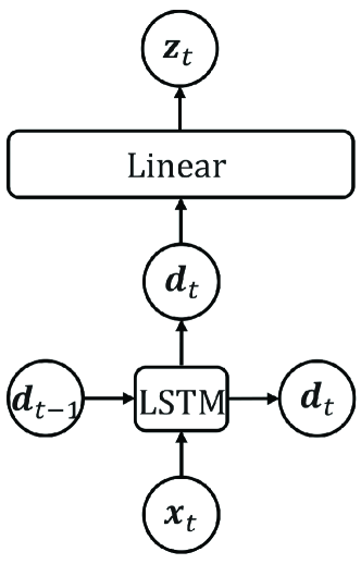
(a) Architecture of $\texttt{SeqEnc}(\cdot;\bm{\Theta}_{\text{SE}})$

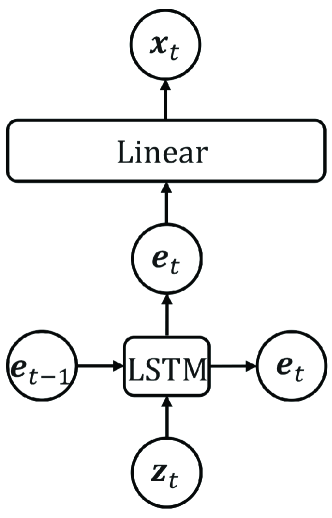
(b) Architecture of $\texttt{SeqDec}(\cdot;\bm{\Theta}_{\text{SD}})$

Figure 3: Instantiate $\texttt{SeqEnc}(\cdot;\bm{\Theta}_{\text{SE}})$ and $\texttt{SeqDec}(\cdot;\bm{\Theta}_{\text{SD}})$.

Instantiation of $\texttt{Predic}(\cdot;\bm{\Theta}_{\text{PD}})$. Again we consider simple instantiations of the predictor $\texttt{Predic}(\cdot;\bm{\Theta}_{\text{PD}})$, to better demonstrate the power of our proposed architecture. We consider three instances of $\texttt{Predic}(\cdot;\bm{\Theta}_{\text{PD}})$.

1. Instantiating $\texttt{Predic}(\cdot;\bm{\Theta}_{\text{PD}})$ using linear transformation. This is the simplest instance of $\texttt{Predic}(\cdot;\bm{\Theta}_{\text{PD}})$. This instance enables us to compare our architecture with the methods based on the Koopman operator theory [21], which uses a linear transformation to capture dependence between latent embeddings. Formally, for a latent embedding sequence ${\bm{Z}}_{t}=[{\bm{z}}_{t-\ell_{h}+1},\cdots,{\bm{z}}_{t}]$, where ${\bm{z}}_{t}$ is a $N$-dimensional vector, the linear transformation predicts the latent embedding vector in the next time slot as

   $$\texttt{Predic}({\bm{Z}}^{h}_{t};\bm{\Theta}_{\text{PD}})={\bm{P}}{\bm{Z}}_{t}\bm{Q},$$ (4)

   where parameters ${\bm{P}}\in\mathbb{R}^{N\times N}$, $\bm{Z}_{t}\in\mathbb{R}^{N\times\ell_{h}}$ and ${\bm{Q}}\in\mathbb{R}^{\ell_{h}}$.

2. Instantiating $\texttt{Predic}(\cdot;\bm{\Theta}_{\text{PD}})$ via LSTM enabled Seq2Seq. We consider a simple nonlinear instantiation of the predictor. This instantiation enables us to understand the impact of nonlinearity on the final detection accuracy of our proposed architecture. Formally, we instantiate $\texttt{Predic}(\cdot;\bm{\Theta}_{\text{PD}})$ with a basic seq2seq neural network complemented with a single LSTM layer. Figure 4 depicts details of this instantiation.

   

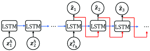
   Figure 4: Instantiate $\texttt{Predic}(\cdot;\bm{\Theta}_{\text{PD}})$ via LSTM Seq2Seq.

3. Instantiating $\texttt{Predic}(\cdot;\bm{\Theta}_{\text{PD}})$ via attention enabled Seq2Seq. This instance of $\texttt{Predic}(\cdot;\bm{\Theta}_{\text{PD}})$ is a little bit more sophisticated than the one depicted in Figure 4. It was shown that seq2seq with attention mechanism is good at capturing temporal dependency and can achieve more accurate prediction [30]. Hence, the purpose of this instance is to understand the impact of the prediction accuracy of Predic on the accuracy of anomaly detectiono in our LPC-AD framework. Formally, this instance of $\texttt{Predic}(\cdot;\bm{\Theta}_{\text{PD}})$ is developed in [30]. Figure 5 shows details on its architecture.

   

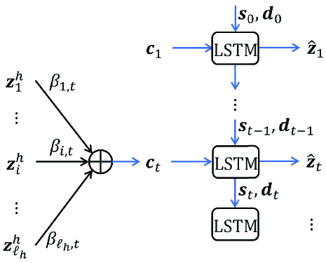
   Figure 5: Instantiate $\texttt{Predic}(\cdot;\bm{\Theta}_{\text{PD}})$ via attention Seq2Seq.

   In Figure 5, the $[\beta_{1,t},\cdots,\beta_{\ell_{h},t}]$ is the attention score vector, which is calculated by the attention function proposed by [5]. Furthermore, we calculate the context vector ${\bm{c}}_{t}$ corresponding to predicted vector $\hat{\bm{z}}_{t}$ as follows:

   $${\bm{c}}_{t}=\beta_{1,t}\times{\bm{z}}^{h}_{1}+\cdots+\beta_{\ell_{h},t}\times{\bm{z}}^{h}_{\ell_{h}},$$ (5)

   where $\beta_{i,t}{=}\exp{l_{i,t}}/(\sum^{\ell_{h}}_{i=1}{\exp{l_{i,t}}}),$ $l_{i,t}{=}{\bm{v}}\tanh({\bm{W}}[{\bm{s}}_{t-1},{\bm{d}}_{d-1}]+{\bm{U}}{\bm{z}}^{h}_{i}),$ and the ${\bm{v}}$, ${\bm{W}}$ and ${\bm{U}}$ are the parameters of the attention function. The attention enabled Seq2Seq can be trained in an end-to-end manner.

Instantiation of randomized perturbation $\texttt{RandPerturb}(\cdot,\bm{\epsilon};\bm{\Theta}_{\text{RP}})$. Again we consider simple instantiations on $\texttt{RandPerturb}(\cdot,\bm{\epsilon};\bm{\Theta}_{\text{RP}})$, to better demonstrate the power of our proposed architecture. Note that $\bm{\epsilon}$ is a zero mean random vector generated from the Gaussian distribution $\mathcal{N}(\bm{0},\bm{\Sigma})$. Formally, we use the following formula to instantiate $\texttt{RandPerturb}(\cdot,\bm{\epsilon};\bm{\Theta}_{\text{RP}})$:

$$\texttt{RandPerturb}({\bm{Z}}_{t+1},\widehat{{\bm{Z}}}_{t+1},\bm{\epsilon};\bm{\Theta}_{\text{RP}})={\bm{Z}}_{t+1}+\bm{\epsilon}\odot({\bm{Z}}_{t+1}-\widehat{{\bm{Z}}}_{t+1})^{\text{abs}},$$

where $\odot$ denotes component-wise multiplication of vectors and $({\bm{Z}}_{t+1}-\widehat{{\bm{Z}}}_{t+1})^{\text{abs}}$ means taking the absolute of each component of the vector ${\bm{Z}}_{t+1}-\widehat{{\bm{Z}}}_{t+1}.$

5.3 Offline Training

We observe that in the loss function $L_{t}(\bm{\Theta})$, the expectation $\mathbb{E}_{\bm{\epsilon}}[\|\widetilde{\bm{W}}_{t+1}-\bm{W}_{t+1}\|_{2}]$ is computationally expensive to evaluate. We use Monte Carlo simulation to address this computational issue. More specifically, we generate $K\in\mathbb{N}_{+}$ samples of the perturbation noise denoted by $\bm{\epsilon}_{1},\ldots,\bm{\epsilon}_{K}$. Let ${\widetilde{\bm{W}}}_{t+1,k}$ denote the reconstructed data associated with $\bm{\epsilon}_{k}$. Formally, we approximate the expectation $\mathbb{E}_{\bm{\epsilon}}[\|\widetilde{\bm{W}}_{t+1}-\bm{W}_{t+1}\|_{2}]$ via $\mathbb{E}[\|\widetilde{\bm{W}}_{t+1}-\bm{W}_{t+1}\|_{2}]\approx\frac{1}{K}\sum\nolimits^{K}_{k=1}\|{\widetilde{\bm{W}}}_{t+1,k}-{\bm{W}}_{t+1}\|_{2}.$ Finally, we use the following approximation on the per time slot loss to train the model:

$$L_{t}(\bm{\Theta}){\approx}\|{\bm{W}}^{h}_{t}{-}{\widehat{\bm{W}}}^{h}_{t}\|_{2}{+}\|{\bm{W}}_{t+1}{-}{\widehat{\bm{W}}}_{t+1}\|_{2}{+}\frac{1}{K}\sum^{K}_{k=1}\!\!\|{\widetilde{\bm{W}}}_{t+1,k}{-}{\bm{W}}_{t+1}\|_{2}.$$ (6)

Based on the above approximated loss, Algorithm 2 outlines our model training procedure.

Algorithm 2 The Generic Training algorithm of LPC-AD

1:$\{({\bm{W}}^{h}_{\ell_{h}},{\bm{W}}_{\ell_{h}+1}),({\bm{W}}^{h}_{\ell_{h}+1},{\bm{W}}_{\ell_{h}+2}),\cdots,({\bm{W}}^{h}_{T-\ell},{\bm{W}}_{T-\ell+1})\}$, number of training rounds $MaxEpoch$.

2:Trained $\bm{\Theta}_{\text{SE}},\bm{\Theta}_{\text{SD}},\bm{\Theta}_{\text{RP}},\bm{\Theta}_{\text{PD}}$

3:Initialize $\bm{\Theta}_{\text{SE}},\bm{\Theta}_{\text{SD}},\bm{\Theta}_{\text{RP}},\bm{\Theta}_{\text{PD}}$

4:$e\leftarrow 1$

5:repeat

6:     for $t=\ell_{h}$ to $T-\ell+1$ do

7:         $[{\bm{Z}}^{h}_{t},\bm{Z}_{t+1}]\leftarrow\texttt{SeqEnc}({\bm{W}}^{h}_{t},\bm{W}_{t+1};\bm{\Theta}_{\text{SE}})$

8:         ${\widehat{\bm{Z}}}_{t+1}\leftarrow\texttt{Predic}({\bm{Z}}^{h}_{t};\bm{\Theta}_{\text{PD}})$

9:         $[{\widehat{\bm{W}}}^{h}_{t},{\widehat{\bm{W}}}_{t+1}]\leftarrow\texttt{SeqDec}({\bm{Z}}^{h}_{t},{{\bm{Z}}}_{t+1};\bm{\Theta}_{\text{SD}})$

10:         for $k=1$ to $K$ do

11:              $\bm{\epsilon}_{k}\sim\mathcal{N}({\bm{0}},{\bm{\Sigma}})$

12:              ${\widetilde{\bm{Z}}}_{t+1,k}\leftarrow\texttt{RandPerturb}(\bm{Z}_{t+1},\widehat{\bm{Z}}_{t+1},\bm{\epsilon}_{k};\bm{\Theta}_{\text{RP}})$

13:              $[*,{\widehat{\bm{W}}}_{t+1,k}]\leftarrow\texttt{SeqDec}({\bm{Z}}^{h}_{t},{\widetilde{\bm{Z}}}_{t+1,k};\bm{\Theta}_{\text{SD}})$

14:         end for

15:         Update $\bm{\Theta}_{\text{SE}}$, $\bm{\Theta}_{\text{SD}}$, $\bm{\Theta}_{\text{PD}}$ and $\bm{\Theta}_{\text{RP}}$ using Eq. (6)

16:     end for

17:     $e\leftarrow e+1$

18:until $e=MaxEpoch$

6 Experiments on Real-World Datasets

In this section, we conduct experiments on four public real-world datasets, which are extensively used to evaluate anomaly detection algorithms. Experiment results show that our proposed LPC-AD algorithm outperforms SOTA algorithms with respect to both detection accuracy and training time.

6.1 Experiment Setting

Device’s Information. We run algorithms on a server, which has a CPU (Intel(R) Xeon(R) Platinum 8151 CPU @ 3.40GHz, 96GB memory) and a GPU (Quadro GV100, 32GB memory).

Public Datasets. We use four public datasets which are extensively used in previous works [36, 40, 42, 4, 37, 18, 9]. Each dataset contains a train set and a testing set. Each data point in the testing dataset has a binary label indicating whether it is an anomaly (1) or not (0). 1 summarizes the overall statistics of each dataset. More details of each dataset are described as follows.

• Server Machine Dataset (SMD). The SMD[36] time series dataset is collected from a large Internet company. Its dimension is 38 and each dimension corresponds to one performance metric of a server. In total, there are 28 time series and each time series corresponds to one server. The horizon of each time series is five weeks. SMD is divided into two subsets of equal size, where the first half is the training set, and the second half with anomaly labels is the testing set.

• Application Server Dataset (ASD). This dataset is also collected from a large Internet company, publiced by [18]. Its dimension is 19 and each dimension corresponds to one performance metric that characterizes the status of a server (CPU-related metrics and memory-related metrics, etc.). In total, there are 12 time series and each time series corresponds to one server. Each time series records a server’s status data in 45 days, with a fixed rate 5 minites. The first 30-day-long data without anomaly labels are used for training, and the last 15-day-long data with anomaly label are used for anomaly testing.

• Secure Water Treatment(SWaT). This dataset is from a real-world industrial water treatment plant producing filtered water [24]. The SWaT dataset is a scaled-down version of the original data. Its dimension is 51, and each dimension corresponds to one performance metric of the industrial water treatment plant. The time horizon of this time series is 11 days. The dataset in the first seven days is collected under normal operations, and that in the last four days is collected with attacks.

• Water Distribution Dataset(WADI). This dataset is collected from the WADI testbed, and it is an extension of the SWaT[2] dataset. Its dimension is 123, and each dimension corresponds to one performance metric of the industrial water treatment plant. It only contains one time series corresponding to one server. The time horizon of this time series is 16 days. The dataset in the first 14 days is collected under normal operations, and that in the last two days is collected with attacks.

Table 1: Statistics of four public datasets.

Dataset	# time series	# metrics	# train	# test	# anomaly(%)
SMD	28	38	708405	708420	4.16
ASD	12	19	102331	51840	4.61
WADI	1	123	784571	172801	5.77
SWaT	1	51	475200	449919	12.13

Comparison baselines. To show the merit of our proposed algorithms, we consider the following SOTA baselines.

• OmniAnomaly[36]. This method is built from a variational autoencoder. Its sophisticated model to capture temporal dependence of time series enhances the detection accuracy, but leads to a slow training speed.

• InterFusion[18]. This method is an improved variant of OmniAnomaly. The improvement is on the detection accuracy of OmniAnomaly. The model is still sophisticated and the training speed is slow.

• USAD[4]. This method achieves a fast training speed by trading-off the detection accuracy. It is built on autoencoder and uses adversarial training.

• TranAD[37]. Similar to USAD, this method focuses on a fast training speed by trading-off detection accuracy. It is built on the transformer architecture.

We do not compare with a number of other notable baselines such as [10, 16, 44, 46], due to that they are shown inferior to TranAD and we omit then for brevity and simplicity of presentation.

To reveal a fundamental understanding of our proposed LPC-AD framework, we consider the following instances of it, where different instances have differet predictors.

• LPC-AD-SA sets the predictor function $\texttt{Predic}(\cdot;\bm{\Theta}_{\text{PD}})$ to be an attention enabled Seq2Seq shown in Figure 5.

• LPC-AD-S sets the predictor function $\texttt{Predic}(\cdot;\bm{\Theta}_{\text{PD}})$ to be a LSTM enabled Seq2Seq shown in Figure 4.

• LPC-AD-L sets the predictor function $\texttt{Predic}(\cdot;\bm{\Theta}_{\text{PD}})$ as a linear function shown in Equation (4).

Evaluation Metrics. Following previous works [36, 40, 42, 4, 37, 18, 9], we use precision, recall, area under the receiver operating characteristic curve (AUROC), and F1 score to evaluate the detection accuracy of all algorithms. We use these metrics that are designed for binary classification because anomaly detection has a binary output, i.e., anomaly (1) or not (0).

In real-world applications, anomalous data points often occur consecutively as an anomalous segment. The purpose of anomaly detection is to notify system operators about the possible issues. Thus, it is acceptable that an anomaly detection algorithm can trigger the anomaly alarm at any subset of a segment of anomalies, instead of correctly classifying each anomalous data points. For this practical consideration, we use a point-adjustment strategy proposed by [40] to calculate the performance metrics. This point-adjustment strategy was widely recognized and applied in previous works [36, 42, 4, 37, 18, 9]. According to this strategy, if at least one data point of an anomalous segment is classified as an anomaly, all the data points of this anomalous segment is considered to be correctly classified as an anomaly.

There are randomness in the training process of these algorithms. The randomness comes from random sampling and random initialization. Faced with such randomness, we repeat the training and testing of each algorithm for $D\in\mathbb{N}_{+}$ times, and take the average results. In some datasets, the number of time series $N$ is more than one. For example, SMD contains 28 time series. To simplify the presentation, we consider the average of the performance metric across all time series in a dataset. Formally, let $P_{i,j},R_{i,j},F_{1,i,j},AUROC_{i,j}$ denote the precision, recall, $F_{1}$ score and receiver operating characteristic curve of the an algorithm on the $i$-th time series of a dataset in the $j$-th repeated training and testing.

$$P=\frac{1}{ND}\sum\nolimits^{N}_{i=1}\sum\nolimits^{D}_{j=1}P_{i,j},\quad R=\frac{1}{ND}\sum\nolimits^{N}_{i=1}\sum\nolimits^{D}_{j=1}R_{i,j},$$ (7)

$$F_{1}=\frac{1}{ND}F_{1,i,j},\quad F^{*}_{1}=2\cdot\frac{P\times R}{P+R},$$ (8)

$$AUROC=\frac{1}{ND}\sum\nolimits^{N}_{i=1}\sum\nolimits^{D}_{j=1}AUROC_{i,j}.$$ (9)

Notably, $F_{1}$ is called the micro $F_{1}$ score and $F^{\ast}_{1}$ is called the macro $F_{1}$ score. In our experiments, we conduct $D=8$ rounds of repeated training and testing, because some baseline algorithms is time-consuming.

Hyperparameter setting & implementation details. For the baseline algorithms (OmniAnomaly, InterFusion, USAD and TranAD), we set their hyperparameters such as window size, embedding size, etc., according to their paper or their open-source code (when it is not stated in the paper). For three instances of LPC-AD, i.e., LPC-AD-SA, LPC-AD-S and LPC-L, we use the following default hyper parameters: historical window size $\ell_{h}=10$, future window size $\ell=2$, hidden layer dimension of LSTM = $M/2$, embedding dimension $N=8(16\text{ for WADI dataset})$, covariance matrix $\bm{\Sigma}=\bm{I}$, learning rate $=0.001$, maximum training epoch $MaxEpoch=40(25\text{ for WADI dataset})$, training batch size$=64$. We also vary the hyperparameters to study their impact on the detection accuracy and training time. By default, we use 100% training dataset for all the algorithms.We implemented instances of LPC-AD with PyTorch-1.9.0 library, trained with Adam optimizer.

All algorithms in consideration detect anomalies based on the alert threshold $\lambda$. Similar with previous works [36, 42, 4, 37, 18, 9], we use exhaustive search to select the optimal alert threshold. In the search, the objective is to achieve the highest $F_{1}$ metric. For instances of LPC-AD, we exhaustively search in [0,1] with a step size of 0.0001. For other baseline algorithms, we use the exhaustive search method stated in their paper.

6.2 Comparison with SOTA Baselines

We first consider the setting where all training data are used for training. We will study the impact of training data size later. We start our evaluation by answering the following question:

Q1: Can LPC-AD improve the detection accuracy and training time compared to the SOTA baselines?

Consider two baselines with sophisticated models with SOTA detection accuracy. Compared with OmniAnomaly, our LPC-AD-SA improves its $F_{1}$ and $F^{\ast}_{1}$ by at least 11.2% over the ASD, WADI and SWaT datasets and by 2.2% over the SMD dataset. It is worth noting that the on the WADI dataset, our LPC-AD-SA improves the $F_{1}$ and $F^{\ast}_{1}$ of OmniAnomaly by around 57.4%. This drastic improvement is due to the fact that the WADI dataset is highly non-smooth, over which the sophisticated model of OmniAnomaly overfits the data. Compared with InterFusion, which is an improved variant of OmniAnomaly, our LPC-AD-SA improves its $F_{1}$ and $F^{\ast}_{1}$ by at most 18.9% over the WADI and SWaT datasets and by at least 2.1% over the SMD and ASD dataset. Namely, LPC-AD-SA significantly outperform the OmniAnomaly and InterFusion in terms of $F_{1}$ and $F^{\ast}_{1}$ For the AUROC accuracy measure, LPC-AD-SA also significantly outperform the OmniAnomaly and InterFusion.

Furthermore, our LPC-AD-SA can significantly outperform these baselines in terms of training speed as well. In particular, Table 3 shows that the per epoch training time of our LPC-AD-SA is less than 10% of that of both OmniAnomaly and InterFusion over four datasets. In other words, the training time of OmniAnomaly and InterFusion are roughly an order of magnitude larger than our LPC-AD-SA.

Answer 1.1: LPC-AD-SA improves the detection accuracy of both OmniAnomaly and InterFusion significantly, and it reduces the training time of both OmniAnomaly and InterFusion drastically.

Table 2: Comparison of detection accuracy with respect to precision($P$), recall($R$) , AUROC, $F_{1}$ and $F^{*}_{1}$ score.

Method	SMD
	P	R	AUROC	$F_{1}$	$F^{*}_{1}$
OmniAnomaly	0.9599	0.9091	0.9539	0.9275	0.9338
InterFusion	0.9262	0.9394	0.9939	0.9287	0.9328
USAD	0.8968	0.9054	0.9499	0.8874	0.9011
TranAD	0.9475	0.9465	0.9954	0.9414	0.947
LPC-AD-SA	0.9401	0.967	0.9973	0.9483	0.9533
Method	ASD
	P	R	AUROC	$F_{1}$	$F^{*}_{1}$
OmniAnomaly	0.8469	0.8593	0.9801	0.8348	0.8531
InterFusion	0.9014	0.9734	0.997	0.9342	0.936
USAD	0.9474	0.8742	0.9906	0.8989	0.9093
TranAD	0.8858	0.9027	0.9846	0.8813	0.8942
LPC-AD-SA	0.9201	0.9539	0.998	0.935	0.9367
Method	WADI
	P	R	AUROC	$F_{1}$	$F^{*}_{1}$
OmniAnomaly	0.6746	0.4587	0.7225	0.537	0.5461
InterFusion	0.7977	0.6589	0.9303	0.7114	0.7217
USAD	0.9293	0.535	0.8966	0.6649	0.6791
TranAD	0.984	0.2405	0.6864	0.3865	0.3865
LPC-AD-SA	0.9369	0.7745	0.9755	0.8455	0.8481
Method	SWaT
	P	R	AUROC	$F_{1}$	$F^{*}_{1}$
OmniAnomaly	0.7241	0.756	0.8519	0.7256	0.7397
InterFusion	0.8495	0.8292	0.9363	0.814	0.8392
USAD	0.9581	0.8625	0.9686	0.9074	0.9078
TranAD	0.9789	0.6963	0.9338	0.8138	0.8138
LPC-AD-SA	0.961	0.9376	0.9926	0.9489	0.9492

Table 3: Comparison of per epoch training time (in seconds).

	SMD	ASD	WADI	SWaT
OmniAnomaly	2945.3	293.4	3937.1	2956.4
InterFusion	2891.6	397.1	2432.8	2076.6
TranAD	304.8	27.3	275.2	168.5
USAD	229.7	31.2	252.3	161.2
LPC-AD-SA	188.1	26.4	209.7	118.2

Consider two baselines with simple models and SOTA training speed, i.e., USAD and TranAD. Table 3 shows that LPC-AD-SA has a shorter per epoch training time than both TranAD and USAD. More specifically, compared with TranAD, our LPC-AD-SA reduces its per epoch running time by at most 38.2% and by at least 24% over the SMD, WADI and SWaT datasets. Over the ASD dataset, LPC-AD-SA reduces the per epoch training time of TranAD by 3.7%. One reason to have this small reduction is that the number of dimension of the ASD dataset is small, i.e., 19, thus TranAD is already fast enough, leaving a small room for further improvement. Compared with USAD, our LPC-AD-SA reduces its per epoch running time by 16%-27% over four datasets. One reason to have this large reduction in training time over all datasets is that the USAD is not fast enough even when the dimension of a dataset is small, leaving a large room for further improvement. These results show that our LPC-AD-SA significantly reduces the running time of TranAD and USAD. Moreover, as shown in Table 2, our LPC-AD-SA can also significantly improve the detection accuracy of TranAd and USAD. In particular, consider the WADI dataset, our LPC-AD-SA improves the $F_{1}$ and $F^{\ast}_{1}$ of both TranAD and USAD by 24.9%-119.42%. On the WADI dataset, LPC-AD-SA improves the AUROC of USAD and TranAD by 8.7% and 42.1%, respectively. One reason to have this drastic improvement is that the WADI is highly non-smooth, over which simple models of TranAD and USAD may under-fit the data, leading to low detection accuracy and leaving a large room for further improvement. For the other three datasets, the time series are smoother than WADI, over which LPC-AD-SA has a smaller improvement (i.e., several percent) of $F_{1}$, $F^{\ast}_{1}$ and AUROC over the TranAD and USAD than the WADI dataset. The reason is that over these datasets, the accuracy of TranAD and USAD is already not low, leaving limited room for further improvement.

Answer 1.2: LPC-AD-SA improves the detection accuracy of both USAD and TranAD significantly, especially when the time series data is highly non-smooth. It also reduces the training time.

Q2: Is the improvement robust to training dataset size?

In order to further validate the superior performance of our LPC-AD-SA over SOTA baselines, we study the impact of training dataset size on the detection accuracy and training time of the algorithms. We use the following method to select a subset of the training dataset. Note that all the algorithms in comparison slice the training time series dataset into sliding windows and then treat each two consecutive window pair as one training data item. When we say a fraction of the training data, such as 50%, we mean randomly selecting 50% of the training data items (i.e. sliding window pairs). This randomness in the selection of training data leads to uncertainty in the output of the algorithm. To eliminate this uncertainty, we repeat each algorithm eight times and take the average as the final output. To simplify the presentation, here, we only consider the SMD dataset. The reason is that, as shown in Table 2, the accuracy improvement of LPC-AD-SA over four SOTA baselines is roughly the smallest among these four datasets. If LPC-AD-SA can still outperform four SOTA baselines in SMD under different training dataset sizes, then one can expect higher improvement over the other three datasets. Another reason is that the SMD datasets has a relatively larger number of time series and has rich temporal patterns in the datasets.

Figure 6(a) shows that as the fraction of the training dataset increases from 10% to 100%, the $F_{1}$ score of LPC-AD-SA and four SOTA baselines increases. Furthermore, the $F_{1}$ curve of LPC-AD-SA lies in the top. This means that LPC-AD-SA has higher $F_{1}$ than four SOTA baselines under different training dataset sizes. The $F_{1}$ curve of LPC-AD-SA is quite flat. This shows that the training accuracy of LPC-AD-SA is robust to training dataset size. This robustness validates the power of LPC-AD-SA in learning the normal temporal dependence. Figure 6(b) and 6(c) shows similar finding with respect to the accuracy measure $F^{\ast}_{1}$ and AUROC. Figure 6(d) shows that as the fraction of the training dataset increases from 10% to 100%, the training time of LPC-AD-SA and four SOTA baselines increases in a nearly linear rate. The training time curve of LPC-AD-SA lies at the bottom. This means that LPC-AD-SA has the fastest training speed than four SOTA baselines under different training dataset sizes. The improvement ratio of train time by the LPC-AD-SA or SOTA baselines across different training dataset sizes varies slightly. In summary, the accuracy of LPC-AD-SA is robust to training dataset size. LPC-AD-SA outperforms four SOTA baselines significantly in terms of both detection accuracy and training time under different selections of training dataset size.

Answer 2: For different training dataset size, LPC-AD-SA robustly improves the detection accuracy and training time over the baselines.

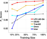
(a) $F_{1}$ score

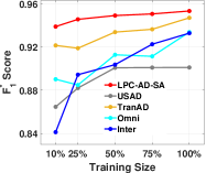
(b) $F^{*}_{1}$ score

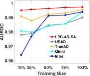
(c) AUROC score

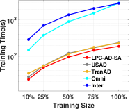
(d) Training time

Figure 6: Impact of training dataset size on the anomaly detection accuracy and training time.

6.3 Parameter Sensitivity Analysis

To reveal fundamental understandings on our proposed LPC-AD algorithm, we now study the anomaly detection accuracy and training time of three instances of LPC-AD under different selections of hyperparameters. Similar with previous works [36, 42, 4, 37, 18, 9], we focus on one dataset, i.e., SMD, for the brevity of presentation. One reason for selecting SMD is that the SMD dataset has a relatively larger number of time series and has rich temporal patterns in the datasets.

Q3: Is LPC-AD robust under different parameter settings?

$\bullet$ Impact of history window size. Figure 7 shows the impact of historical window size $\ell_{h}$ on the detection accuracy and training time on the AutoEncoder baseline (AE) and three instances of LPC-AD. Figure 7(a) shows that the $F_{1}$ curves of LPC-AD-SA, LPC-AD-S and AE are roughly flat as the historical window size $\ell_{h}$ increases from 2 to 3. The same findings can be observed on both the $F^{\ast}_{1}$ and AUROC metric, as shown in Figure 7(b) and 7(c). Namely, the detection accuracy of LPC-AD-SA, LPC-AD-S and AE is not sensitive to the historical window size. Moreover, from Figure 7(a)-7(c), we observe that the detection accuracy of the linear variant LPC-AD-L has a larger variation as the historical window size $\ell_{h}$ changes. Note that the detection accuracy of each algorithm is not monotone in the historical window size. This phenomena that the detection accuracy is not monotone in window size is also observed in the experiments of previous works [4, 18, 37]. One reason of this non-monotonicity is that increasing the historical window size increases the parameters of the model and it does not increase the volume of training data. Figure 7(d) shows that the training time of LPC-AD-SA, LPC-AD-S, LPC-AD-L and AE increases slightly in the historical window size $\ell_{h}$ nearly at a linear rate. This implies that these algorithms scale well with respect to the historical window size $\ell_{h}$. Furthermore, as shown in Figure 7(c), the gap between $F_{1}$ (or AUROC) curves of LPC-AD-SA and LPC-AD-L are quite large. This means that capturing the nonlinear dependence in the time series data can improve the anomaly detection accuracy significantly. Figure 7(d) shows that this improvement in the detection accuracy is achieved at the cost of slowing down the training speed.

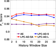
(a) $F_{1}$ score

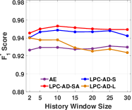
(b) $F^{*}_{1}$ score

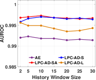
(c) AUROC score

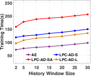
(d) Training time

Figure 7: Impact of historical window size $\ell_{h}$ on the detection accuracy and training time.

$\bullet$ Impact of future window size. Figure 8 shows the impact of future window size $\ell$ on the detection accuracy and training time of three instances of LPC-AD and AE. From Figure 8(a) one can observe that the $F_{1}$ curves of LPC-AD-SA, LPC-AD-S and AE are flat as the historical window size $\ell_{h}$ increases from 1 to 8. Figure 8(b) and 8(c) show similar findings on the $F^{\ast}_{1}$ and AUROC metric. In summary, the detection accuracy of LPC-AD-SA, LPC-AD-S and AE is not sensitive to the historical window size. Figure 8(a)-8(c) show that the detection accuracy of LPC-AD-L decreases in future widow size. The reason that the linear predictor of LPC-AD-L under fits the data, making it less accurate for larger future window size. Figure 8(d) shows that the training time of LPC-AD-SA, LPC-AD-S and LPC-AD-L increases nearly linearly in the future window size $\ell$. Meanwhile, the training time of AE is almost unchanged, because the AE does not have the predictor component. These results show that three instances of LPC-AD scale well with respect to the future window size $\ell$. Lastly, Figure 8 shows similar accuracy vs. training speed tradeoffs as Figure 7, which is caused by capturing the nonlinear temporal dependence in the time series data.

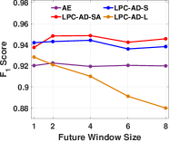
(a) $F_{1}$ score

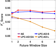
(b) $F^{*}_{1}$ score

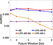
(c) AUROC score

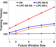
(d) Training time

Figure 8: Impact of future window size on the detection accuracy and training time.

$\bullet$ Impact of latent variable dimension. Figure 9 shows the impact of the dimension $N$ of latent variables on the detection accuracy and training time of the algorithms. Figure 9(a) shows that the $F_{1}$ scores of LPC-AD-SA and LPC-AD-S first increase slightly (less then 3%) when the latent variable dimension increases from 2 to 12. Then they become flat when the latent variable dimension further increases from 12 to 18. The $F_{1}$ of LPC-AD-L and AE varies less than 1% when the latent variable dimension increases from 2 to 18. Figure 9(b) shows similar findings on the $F^{\ast}_{1}$ metric. Furthermore, Figure 9(c) shows that the AUROC of LPC-AD-SA, LPC-AD-S, LPC-AD-L and AE varies less than 1% when the latent variable dimension increases from 2 to 18. In summary, the detection accuracy of LPC-AD-SA, LPC-AD-S and LPC-AD-L are not sensitive to the latent variable dimension. Figure 9(d) shows that the training time of LPC-AD-SA, LPC-AD-S, LPC-AD-L and AE are not sensitive to the dimesion of latent variables. Lastly, Figure 9 shows similar accuracy vs. training speed tradeoffs as Figure 7, which is caused by capturing the nonlinear temporal dependence in MTS.

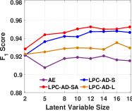
(a) $F_{1}$ score

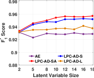
(b) $F^{*}_{1}$ score

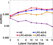
(c) AUROC score

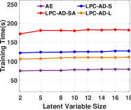
(d) Training time

Figure 9: Impact of latent variable dimension $N$ on the detection accuracy and training time.

$\bullet$ Impact of variance of random perturbation. Note that $\bm{\Sigma}$ is the covariance matrix of the noise of random perturbation. For simplicity of presentation, we consider a special form of $\bm{\Sigma}$, i.e., $\bm{\Sigma}=\sigma^{2}\bm{I},$ where $\sigma^{2}$ measures the variance and $\bm{I}$ is an $N$ dimensional identity matrix. Figure 10 shows the impact of variance $\sigma^{2}$ on the anomaly detection accuracy. We omit the experiment results on training time for brevity, as the variance has an ignorable influence the training time. Figure 10 shows that the $F_{1}$ and AUROC of LPC-AD-SA, LPC-AD-S and LPC-AD-L vary slightly (less than 1%) when the variance $\sigma^{2}$ increases from 0.5 to 4. This shows that LPC-AD-SA, LPC-AD-S and LPC-AD-L are not sensitive to the variance of the noise of random perturbation.

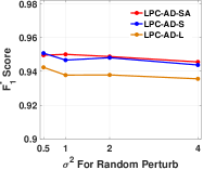
(a) $F^{*}_{1}$ score

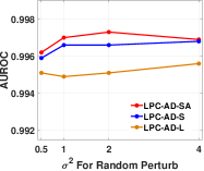
(b) AUROC score

Figure 10: Impact of variance of random perturbation $\sigma^{2}$ on the detection accuracy and training time.

Answer 3: Our LPC-AD-SA algorithm is robust to parameters of history window size, future window size, latent variable dimension and variance of random perturbation.

6.4 Ablation Study

In this subsection, we conduct an ablation study to reveal a fundamental understanding on how two key components of our proposed algorithm, i.e., the predictor and the randomized perturbation operator, improve the anomaly detection accuracy.

Q4: Is it necessary to introduce the predictor and random perturbations?

$\bullet$ Impact of the predictor. Figure 11 shows the $F_{1}$ and AUROC of AE and instances of LPC-AD with different predictors. Note that the AE corresponds to a degenerated variant of LPC-AD by deleting the predictor component. In addition, AE does not have the randomized perturbation operator, as it is built on the predictor. Figure 11 shows that the $F_{1}$ and AUROC of three instances of LPC-AD are always higher than AE over four datasets. Particularly on the WADI dataset, the LPC-AD-L improves the $F_{1}$ and AUROC of AE drastically. This shows that even a simple linear predictor can improve the detection accuracy significantly. One can also observe that the LPC-AD-S has a higher $F_{1}$ and AUROC than LPC-AD-L in most cases. This shows the importance of capturing nonlinearity in the prediction. Moreover, the LPC-AD-SA has a higher $F_{1}$ and AUROC than LPC-AD-S on all four datasets. In summary, there is rich temporal dependence among the latent variables and it is important to use non-linear predictor to capture it well in order to improve the anomaly detection accuracy.

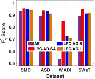
(a) $F^{*}_{1}$ score

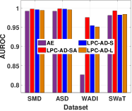
(b) AUROC score

Figure 11: Impact of the predictor on the anomaly detection accuracy.

$\bullet$ Impact of randomized perturbation. To study the impact of randomized perturbation, we consider a variant of LPC-AD without randomized perturbation denoted by LPC-AD-N, where N refers to no randomized perturbation. In particular, LPC-AD-N is obtained by setting the randomized perturbation operator in the following deterministic form $\texttt{RandPerturb}({\bm{Z}}_{t+1},\widehat{{\bm{Z}}}_{t+1},\bm{\epsilon};\bm{\Theta}_{\text{RP}})=\widehat{{\bm{Z}}}_{t+1}.$ Figure 12(a) shows that LPC-AD-SA always have a higher $F_{1}$ than LPC-AD-N, where the improvement reaches a significant number of 5%. Figure 12(b) shows that LPC-AD-SA always has a higher AUROC than LPC-AD-N, except on the WADI dataset. On the WADI dataset, the AUROC of LPC-AD-SA is around 0.5% lower than LPC-AD-N.

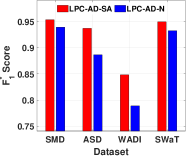
(a) $F^{*}_{1}$ score

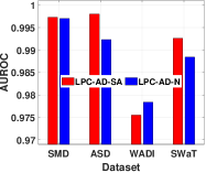
(b) AUROC score

Figure 12: Impact of randomized perturbation on the detection accuracy.

Answer 4: Adding the predictor can increase the F1 score by as high as 9.16%. Adding the randomized perturbation can increase the F1 score by as high as 5%.

7 Conclusion

This paper presents LPC-AD, which has shorter training time than SOTA deep learning methods that focus on reducing training time and it has a higher detection accuracy than SOTA sophisticated deep learning methods that focus on enhancing detection accuracy. These merits of LPC-AD are supported by novelty in the design and extensive empirical evaluations. In particular, LPC-AD contributes a generic architecture LPC-Reconstruct, which is a novel combination of ideas from autoencoder, predictive coding and randomized perturbation. We also contribute a new randomized perturbation method to avoid overfitting of anomalous dependence patterns. Extensive experiments validate superior performance and reveal fundamental understating of our method.

References

- [1] J. Abernethy, C. Lee, and A. Tewari. Perturbation techniques in online learning and optimization. Perturbations, Optimization, and Statistics, page 223, 2016.
- [2] C. M. Ahmed, V. R. Palleti, and A. P. Mathur. Wadi: a water distribution testbed for research in the design of secure cyber physical systems. In Proceedings of the 3rd International Workshop on Cyber-Physical Systems for Smart Water Networks, pages 25–28, 2017.
- [3] B. S. Atal and M. R. Schroeder. Adaptive predictive coding of speech signals. Bell System Technical Journal, 49(8):1973–1986, 1970.
- [4] J. Audibert, P. Michiardi, F. Guyard, S. Marti, and M. A. Zuluaga. Usad: unsupervised anomaly detection on multivariate time series. In Proceedings of the 26th ACM SIGKDD International Conference on Knowledge Discovery & Data Mining, pages 3395–3404, 2020.
- [5] D. Bahdanau, K. Cho, and Y. Bengio. Neural machine translation by jointly learning to align and translate. arXiv preprint arXiv:1409.0473, 2014.
- [6] T. R. Bandaragoda, K. M. Ting, D. Albrecht, F. T. Liu, and J. R. Wells. Efficient anomaly detection by isolation using nearest neighbour ensemble. In 2014 IEEE International conference on data mining workshop, pages 698–705. IEEE, 2014.
- [7] L. Bontemps, V. L. Cao, J. McDermott, and N.-A. Le-Khac. Collective anomaly detection based on long short-term memory recurrent neural networks. In International conference on future data and security engineering, pages 141–152. Springer, 2016.
- [8] S. Chauhan and L. Vig. Anomaly detection in ecg time signals via deep long short-term memory networks. In 2015 IEEE International Conference on Data Science and Advanced Analytics (DSAA), pages 1–7. IEEE, 2015.
- [9] L. Dai, T. Lin, C. Liu, B. Jiang, Y. Liu, Z. Xu, and Z.-L. Zhang. Sdfvae: Static and dynamic factorized vae for anomaly detection of multivariate cdn kpis. In Proceedings of the Web Conference 2021, pages 3076–3086, 2021.
- [10] A. Deng and B. Hooi. Graph neural network-based anomaly detection in multivariate time series. In Proceedings of the AAAI Conference on Artificial Intelligence, volume 35, pages 4027–4035, 2021.
- [11] C. Doersch, A. Gupta, and A. A. Efros. Unsupervised visual representation learning by context prediction. In Proceedings of the IEEE international conference on computer vision, pages 1422–1430, 2015.
- [12] S. Huang, Y. Liu, C. Fung, R. He, Y. Zhao, H. Yang, and Z. Luan. Hitanomaly: Hierarchical transformers for anomaly detection in system log. IEEE Transactions on Network and Service Management, 17(4):2064–2076, 2020.
- [13] K. Hundman, V. Constantinou, C. Laporte, I. Colwell, and T. Soderstrom. Detecting spacecraft anomalies using lstms and nonparametric dynamic thresholding. In Proceedings of the 24th ACM SIGKDD international conference on knowledge discovery & data mining, pages 387–395, 2018.
- [14] K. Kingsbury and P. Alvaro. Elle: Inferring isolation anomalies from experimental observations. arXiv preprint arXiv:2003.10554, 2020.
- [15] G. Kitagawa and W. Gersch. Linear gaussian state space modeling. In Smoothness priors analysis of time series, pages 55–65. Springer, 1996.
- [16] D. Li, D. Chen, B. Jin, L. Shi, J. Goh, and S.-K. Ng. Mad-gan: Multivariate anomaly detection for time series data with generative adversarial networks. In International Conference on Artificial Neural Networks, pages 703–716. Springer, 2019.
- [17] G. Li, X. Zhou, J. Sun, X. Yu, Y. Han, L. Jin, W. Li, T. Wang, and S. Li. opengauss: An autonomous database system. Proceedings of the VLDB Endowment, 14(12):3028–3042, 2021.
- [18] Z. Li, Y. Zhao, J. Han, Y. Su, R. Jiao, X. Wen, and D. Pei. Multivariate time series anomaly detection and interpretation using hierarchical inter-metric and temporal embedding. In Proceedings of the 27th ACM SIGKDD Conference on Knowledge Discovery & Data Mining, pages 3220–3230, 2021.
- [19] D. Liu, C. He, X. Peng, F. Lin, C. Zhang, S. Gong, Z. Li, J. Ou, and Z. Wu. Microhecl: high-efficient root cause localization in large-scale microservice systems. In 2021 IEEE/ACM 43rd International Conference on Software Engineering: Software Engineering in Practice (ICSE-SEIP), pages 338–347. IEEE, 2021.
- [20] F. T. Liu, K. M. Ting, and Z.-H. Zhou. Isolation forest. In 2008 eighth ieee international conference on data mining, pages 413–422. IEEE, 2008.
- [21] B. Lusch, J. N. Kutz, and S. L. Brunton. Deep learning for universal linear embeddings of nonlinear dynamics. Nature communications, 9(1):1–10, 2018.
- [22] M. Ma, Z. Yin, S. Zhang, S. Wang, C. Zheng, X. Jiang, H. Hu, C. Luo, Y. Li, N. Qiu, et al. Diagnosing root causes of intermittent slow queries in cloud databases. Proceedings of the VLDB Endowment, 13(8):1176–1189, 2020.
- [23] P. Malhotra, A. Ramakrishnan, G. Anand, L. Vig, P. Agarwal, and G. Shroff. Lstm-based encoder-decoder for multi-sensor anomaly detection. arXiv preprint arXiv:1607.00148, 2016.
- [24] A. P. Mathur and N. O. Tippenhauer. Swat: A water treatment testbed for research and training on ics security. In 2016 international workshop on cyber-physical systems for smart water networks (CySWater), pages 31–36. IEEE, 2016.
- [25] J. R. Medel and A. Savakis. Anomaly detection in video using predictive convolutional long short-term memory networks. arXiv preprint arXiv:1612.00390, 2016.
- [26] Y. Meng, S. Zhang, Y. Sun, R. Zhang, Z. Hu, Y. Zhang, C. Jia, Z. Wang, and D. Pei. Localizing failure root causes in a microservice through causality inference. In 2020 IEEE/ACM 28th International Symposium on Quality of Service (IWQoS), pages 1–10, 2020.
- [27] T. Mikolov, K. Chen, G. Corrado, and J. Dean. Efficient estimation of word representations in vector space. arXiv preprint arXiv:1301.3781, 2013.
- [28] D. Park, Y. Hoshi, and C. C. Kemp. A multimodal anomaly detector for robot-assisted feeding using an lstm-based variational autoencoder. IEEE Robotics and Automation Letters, 3(3):1544–1551, 2018.
- [29] A. Patcha and J.-M. Park. An overview of anomaly detection techniques: Existing solutions and latest technological trends. Computer networks, 51(12):3448–3470, 2007.
- [30] Y. Qin, D. Song, H. Chen, W. Cheng, G. Jiang, and G. Cottrell. A dual-stage attention-based recurrent neural network for time series prediction. arXiv preprint arXiv:1704.02971, 2017.
- [31] S. Ren, D. Li, Z. Zhou, and P. Li. Estimate the implicit likelihoods of gans with application to anomaly detection. In Proceedings of The Web Conference 2020, pages 2287–2297, 2020.
- [32] D. A. Reynolds. Gaussian mixture models. Encyclopedia of biometrics, 741(659-663), 2009.
- [33] D. Rezende and S. Mohamed. Variational inference with normalizing flows. In International conference on machine learning, pages 1530–1538. PMLR, 2015.
- [34] M. Sakurada and T. Yairi. Anomaly detection using autoencoders with nonlinear dimensionality reduction. In Proceedings of the MLSDA 2014 2nd Workshop on Machine Learning for Sensory Data Analysis, MLSDA’14, page 4–11, New York, NY, USA, 2014. Association for Computing Machinery.
- [35] N. Srivastava, E. Mansimov, and R. Salakhudinov. Unsupervised learning of video representations using lstms. In International conference on machine learning, pages 843–852. PMLR, 2015.
- [36] Y. Su, Y. Zhao, C. Niu, R. Liu, W. Sun, and D. Pei. Robust anomaly detection for multivariate time series through stochastic recurrent neural network. In Proceedings of the 25th ACM SIGKDD international conference on knowledge discovery & data mining, pages 2828–2837, 2019.
- [37] S. Tuli, G. Casale, and N. R. Jennings. Tranad: Deep transformer networks for anomaly detection in multivariate time series data. arXiv preprint arXiv:2201.07284, 2022.
- [38] A. Vaswani, N. Shazeer, N. Parmar, J. Uszkoreit, L. Jones, A. N. Gomez, Ł. Kaiser, and I. Polosukhin. Attention is all you need. Advances in neural information processing systems, 30, 2017.
- [39] Y. Wang, N. Masoud, and A. Khojandi. Real-time sensor anomaly detection and recovery in connected automated vehicle sensors. IEEE transactions on intelligent transportation systems, 22(3):1411–1421, 2020.
- [40] H. Xu, W. Chen, N. Zhao, Z. Li, J. Bu, Z. Li, Y. Liu, Y. Zhao, D. Pei, Y. Feng, et al. Unsupervised anomaly detection via variational auto-encoder for seasonal kpis in web applications. In Proceedings of the 2018 world wide web conference, pages 187–196, 2018.
- [41] A. H. Yaacob, I. K. Tan, S. F. Chien, and H. K. Tan. Arima based network anomaly detection. In 2010 Second International Conference on Communication Software and Networks, pages 205–209. IEEE, 2010.
- [42] C. Zhang, D. Song, Y. Chen, X. Feng, C. Lumezanu, W. Cheng, J. Ni, B. Zong, H. Chen, and N. V. Chawla. A deep neural network for unsupervised anomaly detection and diagnosis in multivariate time series data. In Proceedings of the AAAI conference on artificial intelligence, volume 33, pages 1409–1416, 2019.
- [43] R. Zhang, P. Isola, and A. A. Efros. Colorful image colorization. In European conference on computer vision, pages 649–666. Springer, 2016.
- [44] H. Zhao, Y. Wang, J. Duan, C. Huang, D. Cao, Y. Tong, B. Xu, J. Bai, J. Tong, and Q. Zhang. Multivariate time-series anomaly detection via graph attention network. In 2020 IEEE International Conference on Data Mining (ICDM), pages 841–850. IEEE, 2020.
- [45] Y. Zhao, B. Deng, C. Shen, Y. Liu, H. Lu, and X.-S. Hua. Spatio-temporal autoencoder for video anomaly detection. In Proceedings of the 25th ACM international conference on Multimedia, pages 1933–1941, 2017.
- [46] B. Zong, Q. Song, M. R. Min, W. Cheng, C. Lumezanu, D. Cho, and H. Chen. Deep autoencoding gaussian mixture model for unsupervised anomaly detection. In International conference on learning representations, 2018.