Explanation-Guided Fairness Testing through Genetic Algorithm

Abstract.

The fairness characteristic is a critical attribute of trusted AI systems. A plethora of research has proposed diverse methods for individual fairness testing. However, they are suffering from three major limitations, i.e., low efficiency, low effectiveness, and model-specificity. This work proposes ExpGA, an explanation-guided fairness testing approach through a genetic algorithm (GA). ExpGA employs the explanation results generated by interpretable methods to collect high-quality initial seeds, which are prone to derive discriminatory samples by slightly modifying feature values. ExpGA then adopts GA to search discriminatory sample candidates by optimizing a fitness value. Benefiting from this combination of explanation results and GA, ExpGA is both efficient and effective to detect discriminatory individuals. Moreover, ExpGA only requires prediction probabilities of the tested model, resulting in a better generalization capability to various models. Experiments on multiple real-world benchmarks, including tabular and text datasets, show that ExpGA presents higher efficiency and effectiveness than four state-of-the-art approaches.

1. Introduction

Artificial Intelligence (AI) systems have been penetrating various aspects of our lives. Except for the benefits brought by AI systems, however, an AI system would harm the fairness of our society if it makes biased decisions and thus presents a discriminatory nature. Recent studies (Buolamwini and Gebru, 2018; Tatman, 2017) pointed out that some familiar AI systems behave with deviations in gender and skin color. For example, in face recognition systems developed by IBM, Microsoft, and face++, the detection accuracy for white-skin men is much higher (sometimes 20% higher) than that of black-skin women.

Fairness characteristic is critical for trusted AI systems, and fairness testing has attracted much attention recently in both industrial (e.g., IBM’s AI Fairness 360 (AI3, 2021), Google’s ML-Fairness-Gym (Fai, 2021)) and academic communities (Mehrabi et al., 2019; Saxena, 2019; Tramer et al., 2017). The GDPR (GDP, 2021), a data privacy law across Europe, claims that “the personal data shall be processed fairly in relation to the data subject”. Definitions of fairness in existing work fall into two categories (Mehrabi et al., 2019): 1) individual fairness, i.e., similar individuals are given similar decisions; 2) group fairness, i.e., equal decisions are made for different groups. Most research on software fairness, including this work, has focused on individual fairness (Brun and Meliou, 2018).

Individual fairness testing mutates the input samples to generate sufficient testing samples and checks whether these samples are individual-discriminatory. Typical approaches include THEMIS (Galhotra et al., 2017), AEQUITAS (Udeshi et al., 2018), SG (Aggarwal et al., 2019), ADF (Zhang et al., 2020), and MT-NLP (Ma et al., [n.d.]). In general, these fairness testing methods first construct a set of seed samples that are suspiciously discriminatory using random or clustering techniques. Then, they search for more discriminatory samples around the seeds through different strategies, such as symbolic execution and gradient-based methods. After that, they expand the original dataset by modifying the labels of detected discriminatory samples and finally retrain to improve the model fairness. Prior individual fairness testing approaches have achieved relatively good performance; however, they still suffer from three major limitations.

Low efficiency: When handling complex deep learning systems, SG (Aggarwal et al., 2019) is inefficient due to the use of symbolic execution. Symbolic execution, which typically requires SMT solvers, is computationally expensive to generate particular test cases.

Low effectiveness: THEMIS (Galhotra et al., 2017), AEQUITAS (Udeshi et al., 2018), and MT-NLP (Ma et al., [n.d.]) adopt unguided or semi-guided search strategies, leading to a low success rate of the discriminatory sample generation.

Model-specificity: ADF (Zhang et al., 2020), a lightweight approach, requires gradient information. Such information is extracted from the white-box DNN model but unavailable in black-box models.

To address these limitations, this work proposes ExpGA, a model-agnostic fairness testing approach. ExpGA employs explanation results and the genetic algorithm (GA), thus detecting discriminatory samples both efficiently and effectively.

Our ExpGA first leverages the explanation results generated by interpretable methods to identify a set of seed samples. Seed samples are prone to derive discriminatory samples by slightly modifying their feature values. Then, using seed samples as the input, ExpGA employs the GA to produce large amount of discriminatory offspring. In ExpGA, the explanation results favor high-quality seeds. GA can guide the search process towards discriminatory sample solutions by optimizing the fitness value. Furthermore, ExpGA is able to handle black-box models since it only requires prediction probabilities from the models.

To evaluate the efficiency and effectiveness of our ExpGA, we compare ExpGA with four state-of-the-art discriminatory testing approaches, including AEQUITAS, SG, ADF, and MT-NLP. Using five diverse training models, we conduct comprehensive experiments on three tabular dataset benchmarks (handled by AEQUITAS, SG, and ADF) and two text dataset benchmarks (handled by MT-NLP). The data of our experiments can be found on github.

The results indicate that ExpGA can detect discriminatory samples more efficiently and effectively than the baseline approaches. In particular, on tabular datasets, ExpGA consumes less than 0.2s to identify a discriminatory sample with a success rate of 49% on average, outperforming AEQUITAS, SG, and ADF in both efficiency and accuracy. On text datasets, ExpGA is five times more efficient and twice more effective than MT-NLP. In addition, the performance of ExpGA is more stable in various models than the four baseline approaches, indicating a better generalization capability of ExpGA.

In summary, our work makes the following contributions:

1. We propose a model-agnostic fairness testing approach called ExpGA. It can identify individual discriminatory samples for both tabular data and text data by combining the local explanation and GA.

2. We conduct extensive experiments on three tabular datasets and two text datasets to evaluate ExpGA. The results show that ExpGA outperforms four state-of-the-art approaches in terms of both efficiency and effectiveness.

Figure 1. An example pair of discriminatory samples

In the rest of this paper: Section 2 introduces the background and the problem definition. Section 3 illustrates ExpGA and Section 4 reports experimental results. Section 5 and 6 discuss the threats to validity and related work. Section 7 draws conclusions.

2. Background and Problem Definition

2.1. Individual Discrimination

There exists individual discrimination in a classifier if some protected attributes explicitly play important roles in the decision-making process (Mitchell et al., 2018; Corbett-Davies and Goel, 2018). The protected attributes are predefined in specific domains such as gender, country, and age.

Formally, given a classifier $f=<X,A>$, $X$ denotes the input domain, and $A={A_{1}}\times{A_{2}}\times\cdots\times{A_{n}}$ represents the feature space of $X$. Each input sample $x\in X$ is represented as a n dimensional feature vector, i.e., $x=\left\{{{a_{1}},{a_{2}},\ldots,{a_{n}}}\right\}$. Considering a set of protected attributes $P$, a classifier $f$ presents individual discrimination if there exists a pair of samples, $x$ and $x^{\prime}$, satisfying the following Eq. (1)-(3), where ${x=\{a_{1},a_{2},...,a_{n}\}}$ and ${x^{{}^{\prime}}}=\{{{a_{1}^{{}^{\prime}}},{a_{2}^{{}^{\prime}}},\ldots,{a_{n}^{{}^{\prime}}}}\}$. In this case, $x$ and $x^{{}^{\prime}}$ are a pair of discriminatory samples in $f$. Here we use the symbols $\rhd$ and $\unrhd$ to denote that one feature is closely related and unrelated to a specific protected attribute, respectively.

(1) $$\small\exists a_{i}\in x,a_{i}\rhd p\in P,a_{i}\neq a^{\prime}_{i}$$

(2) $$\small\forall a_{j}\in x,a_{j}\unrhd p\in P,a_{j}=a^{\prime}_{j}$$

(3) $$\small f(x)\neq f({x^{{}^{\prime}}})$$

Fig. 1 presents an example pair of discriminatory samples that are classified into different classes. The only difference between the two samples is their values of sex feature, which is related to the protected attribute gender, indicating the unfairness of the classifier with regard to gender. Note that the approach of ignoring certain protected attributes to mitigate model bias is not effective due to the presence of redundant encoding in the training dataset (Pedreshi et al., [n.d.]).

2.2. Locally Interpretable Method

The drawbacks of invisible black-box models raise a series of security issues; many studies have proposed interpretable methods to measure the credibility of the prediction process. Among them, the locally interpretable methods (Guo et al., 2018; Ribeiro et al., 2018, 2016; Lundberg and Lee, 2017; Guidotti et al., 2018) are the most prominent. They interpret the predictions of black-box classifier models by providing potentially important features that dominate the decision results. By approximating the decision boundary of the classifier model, the generated interpreter learned with interpretable methods can explain the prediction specifically for a single sample. Concretely, given a test sample $x$, and its classification result $y=f(x)$, an interpreter $g$ will output explanation results $e$, a sorted set of features ranking based on their importance to this decision result.

2.3. Genetic Algorithm

The genetic algorithm (GA) is commonly used to search for approximate optimal solutions (Mishra et al., 2019; Zhang and Tao, 2017; Sharma et al., 2016). GA first randomly initializes a population with potential solutions to the target problem. It then approximates the optimal solution iteratively through three biologically inspired operators, including selection, crossover, and mutation.

Specifically, GA encodes each solution in the initial population into a set of “gene” sequences and designs a fitness function to measure the qualities of current solutions. In the selection step, solutions with better fitness scores tend to be selected into the new population. In the crossover step, two parent solutions’ gene fragments are exchanged to produce children solutions. After that, a part of gene fragments of children solutions are mutated randomly, probably breaking out of the local search space and enhancing the diversity of solutions. GA repeats the whole process until a desirable solution is found or the number of iterations reaches the maximum as configured.

2.4. Problem Definition

For a given model, if the input is identified as an individual discriminatory sample, this model would be suffered from individual discrimination and may produce a biased decision. In this software fairness testing work, we assume that the dataset $X$ for training a model, the corresponding feature space $A$, and the protected attribute set $P$ are provided. The problem is that, given a black-box model $D$ trained using dataset $X$, can we effectively and efficiently detect individual discriminatory samples for $D$? By supplementing the discovered individual discriminatory samples to $X$, the model fairness is desired to have an improvement through retraining. We have no prior knowledge (i.e., training algorithms and parameters) about the black-box model, making existing white-box based methods that require model inner information ineffective.

3. Methodology

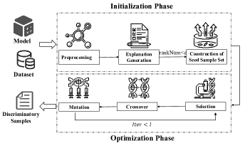
Figure 2. The overview of ExpGA.

In this paper, we propose the ExpGA, a lightweight model-agnostic software fairness testing method. Fig. 2 illustrates the overall framework of ExpGA. The inputs are a dataset and its trained model. In the initialization phase, ExpGA employs an interpretable method to search for seed samples in the entire feature domain. Seed samples are more likely to derive discriminatory samples by slightly modifying feature values than other samples. Using seeds as inputs, the optimization phase employs GA to efficiently generate a large number of discriminatory samples through the selection, crossover, and mutation operators.

To illustrate the generalizability of ExpGA, we present two diverse scenarios that ExpGA is able to handle: the input dataset is a tabular form or a set of text paragraphs. Fig. 3 shows the two corresponding examples. The first example is selected from the census income classification dataset (Cen, 2021), as shown in Fig. 3(a). Each sample includes features of marital status, sex, occupation, education, hours per week, etc. The labels of sample 1 and sample 2 are Income$>$50k and Income$\leq$50k, respectively. Another example is selected from the sentiment analysis dataset for movie comments (i.e., IMDB dataset (IMD, 2021)). As shown in Fig. 3(b), each sample in this dataset is a text paragraph. Although the samples in the above two different scenarios are heterogeneous, they both can be consistently represented as feature vectors, $x=\{a_{1},a_{2},\dots,a_{n}\}$. For tabular samples, $a_{i}$ denotes the $i$-th feature value; for text samples, $a_{i}$ denotes the $i$-th word. For convenience, we will uniformly use $a_{i}$ to denote the $i$-th word of sample $x$.

Figure 3. Two examples in tabular dataset and text dataset scenarios.

3.1. Initialization Phase

The initialization phase first identifies whether a sample contains sensitive words that are related to the given protected attributes $P$. Then it learns an interpreter by employing the interpretable methods, outputting the words that dominate decision results. The samples whose sensitive word ranks high in these explanation results are selected as the seed samples. Concretely, this phase contains three steps, i.e., prepossessing, explanation generation, and construction of the seed sample set.

3.1.1. Preprocessing

This step will identify the sensitive words that are related to the protected attributes. Considering that the protected attribute is $\{gender\}$, we can easily identify that the word “sex” in Fig. 3(a) is definitely close to the attribute since they present a similar semantic meaning. However, in some cases like Fig. 3(b), it is difficult to literally decide the relationships between the words and protected attributes due to the diversity of the language. In this example, the word “master” might be related to the gender information implicitly.

To solve this problem, we manually construct a knowledge graph containing the relations between sensitive words and protected attributes. At first, we obtain the protected attributes following an existing work (Corbett-Davies and Goel, 2018; Foulds et al., 2020; Pro, 2021). Then, we construct a set of general relations, such as “IsA”, “RelatedTo”, “DistinctFrom”, according to the ConceptNet (Con, 2021), a widely used, open, and multilingual knowledge graph. After that, we expand the graph by adding similar words with a word embedding tool such as Glove (Pennington et al., 2014). For a new word, if there exists a similar word in the graph of which the similarity surpasses the configured threshold (i.e., 0.7), it will be added to the graph. Finally, once a word has an accessible path to the protected attribute in the graph, it is regarded as a sensitive word that is related to the specific protected attribute. Note that the knowledge graph only needs to be constructed once.

Fig. 4 depicts a sub-graph of the knowledge graph we have constructed. The sub-graph contains a subset of protected attributes, such as gender, age, country, and religion. An edge of this graph indicates a relation from a subject to an object. For instance, America “IsA” a country. Based on this graph, for the example shown in Fig. 3(b), we can identify that “master” is a person and it has the gender attribute. Thus, it is identified as a sensitive word related to gender, that is, $master\rhd gender$.

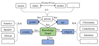
Figure 4. A partial prior knowledge graph.

3.1.2. Explanation Generation

Our assumption of using interpretable methods is that non-sensitive words should have a synergistic influence, dominating the classification of samples without discrimination. On the contrary, for discrimination samples, their sensitive words would rank relatively high in explanation results. As a result, a slight perturbation of sensitive words on discrimination samples might dramatically change the predicted label. Furthermore, we rely on the model-agnostic interpretable methods since they are good at training an interpreter for an opaque model, thus benefiting the generalization of ExpGA to different models such as CNN, MLP, and SVM.

Fig. 5 presents the explanation results for the two examples in Fig. 3. The words “male” and “master” are marked with red color since they are identified as sensitive words during the prepossessing step. The darker blue shading words play more essential roles in the classification process than the lighter shading words.

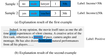
Figure 5. Explanation results of the two examples.

Input: $X$, $P$, Classifier $f$, Interpreter $g$, $seed\_num$, $\epsilon$,

Output: Seed Sample Set $SeedSet$

1 $SeedSet=\emptyset$

2 foreach sample $x$ in $X$ do

3       if $|SeedSet|\leq seed\_num$ then

4             $label=f(x)$

5             $e=g(x,f,label)$

6             foreach $a_{i}$ in $x$ do

7                   if $a_{i}\rhd p,p\in P$ then

8                         $r=rankNum(a_{i},e)$

9                         if $r\leq\epsilon$ then

10                               $SeedSet=SeedSet\cup\{x\}$

11                        

12                  

13            

14      

return $SeedSet$

Algorithm 1 Initialization phase

3.1.3. Construction of Seed Sample Set

This step constructs a set of seed samples, from which more discriminatory samples will be derived by the genetic algorithm. We first rank the explanation result $e$ based on the importance score assigned by the interpretable method. Then we design a function $rankNum(a_{i},e)$ to obtain the rank number of a word $a_{i}$ in $e$. By iteratively obtaining the rank number of each sensitive word, we select the highest number to check whether it is higher than a threshold value $\epsilon$. If higher, the sample will be added to the seed sample set.

$\epsilon$ controls the balance between the number and quality of the selected seed samples. In Fig. 5, given that $\epsilon=2$, all samples are selected as seed samples since the rank numbers of sensitive words contained in these samples are 2. However, if $\epsilon=1$, none of them would be selected. It can be seen that a bigger $\epsilon$ would result in more seed samples; however, the rank number of sensitive words might be lower, making the sensitive words less important. Therefore, the quality of these samples would be poor. On the contrary, a smaller $\epsilon$ can result in high-quality seed samples with a smaller number, which might affect the efficiency of the generation of final discriminatory samples.

Algorithm 1 formalizes the initialization implementations. The inputs include the dataset $X$, protected attribute set $P$, an interpreter $g$ constructed by leveraging the existing interpretable method, and the target number of seed samples ($seed\_num$). The output is a set of seed samples, denoted as $SeedSet$. Each sample is first fed to the classifier and interpreter to generate its explanation results (lines 2-5). The sample, which contains any sensitive word with a smaller ranking number than $\epsilon$, will be added to $SeedSet$ (lines 6-10).

3.2. Optimization Phase

Input: $SeedSet$, $l$

Output: Discriminatory Sample Set $DisSet$

1 $CurPopulation=InitPopulation(SeedSet)$

2 $num=0$

3 while $num\leq l$ do

4       $NewPopulation=Selection(CurPopulation)$

5       $CurPopulation=Crossover(CurPopulation)$

6       $CurPopulation=Mutator(CurPopulation)$

7       foreach sample $x$ in $CurPopulation$ do

8             if $True==DiscrniminatoryCheck(x)$ then

9                   $DisSet=DisSet\cup\{x\}$

10            

11      

return $DisSet$

Algorithm 2 Optimization phase

The optimization phase leverages the biologically inspired GA to generate discriminatory samples, taking advantage of its high convergence speed and strong local searching ability. Here we use Algorithm 2 to help understand the order of the three operators. At first, we will construct the initial population based on the $SeedSet$ input (line 1). Then, the complete process of the selection, crossover, and mutation (lines 4-6) will be repeated $l$ times, as set by users. After finishing each iteration, we leverage $DiscrniminatoryCheck()$ to check whether a candidate sample $x$ is a true discriminatory sample. If the output set $DisSet$ does not contain the sample, $x$ will be added to the set (lines 7-9). The details of the above steps are introduced below.

3.2.1. Construction of Initial Population

This step constructs the initial population based on seed samples. However, it is different to construct the initial populations for the tabular dataset and the text dataset.

For seed samples from a tabular dataset, all of them will be added to the initial population since they have the same number of features.

For seed samples from a text dataset, it is unfeasible to initialize the population by simply aggregating all seed samples since the lengths of paragraphs in different text samples are diverse. A simple replacement of a word $a_{i}$ in one sample with that word $a^{\prime}_{i}$ in another sample (in the next crossover step) would lead to a new sentence with syntax errors or incorrect semantic. In this work, we construct an initial population correspondingly from each seed sample. Specifically, for a given seed sample, we first randomly select $k$ non-sensitive words from it. Correspondingly, $k$ new words that have similar meanings with those $k$ selected words can be obtained through the similarity computation by the word embedding tool Glove. After that, we replace the originally selected words with these new words, producing $k$ new samples derived from the seed sample. The set of these $k+1$ samples will form an initial population. Our work sets $k=20$ according to experimental experience.

3.2.2. Selection

This step selects high-quality samples to generate the next population through optimizing a fitness function. We design a fitness function $fit(x)$ for a sample $x$. $fit(x)$ quantifies the extent of a change from the prediction probability of $x^{\prime}$ to that of $x^{\prime\prime}$. $x^{\prime}$ and $x^{\prime\prime}$ are derived from $x$. We assume that $x$ with a higher fitness score is more likely to be mutated into a discriminatory sample. $fit(x)$ can be obtained with Eq. (4):

(4) $$\small fit(x)=|Prob(x^{\prime},l)-Prob(x^{\prime\prime},l)|$$

We now introduce how to derive $x^{\prime}$ and $x^{\prime\prime}$ from $x$. Given that $x$ contains a sensitive word $a_{i}\rhd p$, we construct the $<\widetilde{a_{i}},\neg\widetilde{a_{i}}>$ that is a pair of sensitive words but with opposite semantic meanings. We then substitute $\widetilde{a_{i}}$ and $\neg\widetilde{a_{i}}$ for the original $a_{i}$, producing two new samples, $x^{\prime}$ and $x^{\prime\prime}$, respectively. $Prob(x^{\prime},l)$ and $Prob(x^{\prime\prime},l)$ correspond to the prediction probability of $x^{\prime}$ and $x^{\prime\prime}$ for the specific label $l$.

For example, given $a_{i}$=“actor” and $p$=gender, $\widetilde{a_{i}}$ is the same as $a_{i}$, and $\neg\widetilde{a_{i}}$ would be “actress”. Another example is that, when $a_{i}$= “master”, $p$=gender, and $a_{i}$ has a relationship with $p$, we would set $\widetilde{a_{i}}=$“male master” and $\neg\widetilde{a_{i}}$=“female master” based on the prior knowledge graph we have constructed in Section 3.1.1.

Algorithm 3 shows the selection in terms of $fit(x)$. The input is current population $CurPopulation$ and the output is a new population $NewPopulation$ after selection. $sumFit$ denotes the sum of all fitness scores of the samples in $CurPopulation$. $\delta(x)$ denotes the probability value of $x$ that might be selected into the new population. $\Delta(X)$ is a set of all $\delta(x)$ of samples in $CurPopulation$. Finally, selecting based on the probability distribution indicated from $\Delta(X)$, we can construct a new population that has the same sample size as $Curpopulation$.

Input: $CurPopulation$

Output: $NewPopulation$

1 $NewPopulation=\emptyset$

2 $sumFit=\sum_{x\in CurPopulation}{fit(x)}$

3 $\Delta(X)=\emptyset$

4 foreach sample $x$ in $CurPopulation$ do

5       $\delta(x)=fit(x)/sumFit$

6       $\Delta(X)=\Delta(X)\cup\delta(x)$

7      

8while $|NewPopulation|<|CurPopulation|$ do

9       $z=select(CurPopulation,\Delta(X))$

10       $NewPopulation=NewPopulation\cup z$

return $NewPopulation$

Algorithm 3 Selection of new population

Input: $CurPopulation$, $cr$, $mr$

Output: $CurPopulation$

1 foreach sample $x$ in $CurPopulation$ do

2       $x^{\prime}=randomSelect(CurPopulation)$

3       $<a_{i},\dots,a_{j}>=randomSelect(x,cr)$

4       $frag(x,i,j)=<a_{i},\dots,a_{j}>$

5       $x=x.replace(frag(x,i,j),frag(x^{\prime},i,j))$

6       $x^{\prime}=x^{\prime}.replace(frag(x^{\prime},i,j),frag(x,i,j))$

7      

8foreach sample $x$ in $CurPopulation$ do

9       foreach $a_{i}$ in $x$ do

10             if $a_{i}\unrhd p$  then

11                  //$\unrhd$ denotes that $a_{i}$ is not related to $p$

12                   $a^{\prime}_{i}=calSimilarWord(a_{i},mr)$

13                   $x=x.replace(a_{i},a^{\prime}_{i})$

14                  

15            

16      

return $CurPopulation$

Algorithm 4 Crossover and Mutation

3.2.3. Crossover and Mutation

We conduct the crossover and mutation operators on the selected population to generate more varieties, expanding the search space of discriminatory samples. Algorithm 4 illustrates the crossover (lines 1-6) and the mutation (lines 7-12). The two parameters, $cr$ and $mr$, denote the crossover rate and mutation rate.

We randomly choose pairs of samples as the crossover parents from the current population with a probability of $cr$. For a pair of samples, $x$ and $x^{\prime}$, fragments $<a_{i},\dots,a_{j}>$ and $<a^{\prime}_{i},\dots,a^{\prime}_{j}>$ are extracted from $x$ and $x^{\prime}$ randomly. The two samples will exchange their fragments with each other.

During the mutation, each word of a sample in the current population is replaced with its similar word with a probability of $mr$. Note that the mutation excludes the sensitive words. Concretely, 1) categorical word such as “no” and “teacher” will be replaced with similar words in the same category such as “yes” and “lawyer”; 2) text word such as “great” and “brilliantly” will be replaced with similar words using the tool Glove; 3) numeric word such as “1” and “36h” can be replaced with numeric data like “2” and “40h”.

Input: $x$, Classifier $f$, $P$

Output: $Dis$

1 $Dis=false$

2 if $\exists a_{i}\in x,a_{i}\rhd p,p\in P$ then

3       $<\widetilde{a_{i}},\neg\widetilde{a_{i}}>=getPair(a_{i})$

4       $x^{\prime}=x.replace(a_{i},\widetilde{a_{i}})$

5       $x^{\prime\prime}=x.replace(a_{i},\neg\widetilde{a_{i}})$

6       if $f(x^{\prime})\neq f(x^{\prime\prime})$ then

7             $Dis=true$

8            

9      

return $Dis$

Algorithm 5 Checking of discriminator sample

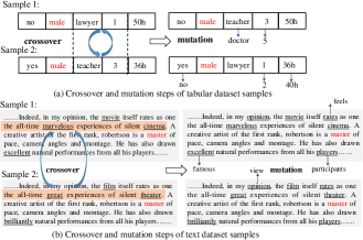
Figure 6. Examples for the crossover and mutation steps.

Fig. 6(a) shows the crossover and mutation for the tabular samples and Fig. 6(b) for the text samples. In Fig. 6(a), the crossover fragments are $<$“lawyer”,“1”$>$ in sample 1 and $<$“teacher”,“3”$>$ in sample 2. Then the words of “teacher”, “3”, “yes”, “1”, and ‘”36h” are mutated with “doctor”, “5”, “no”, “2”, and “40h”. In 5(b), the different words between the two samples are underlined. The two sub-sentences in the orange shading are exchanged with each other. After that, some words like “excellent” will be mutated with their similar words like “famous”.

3.2.4. Checking of Discriminatory Sample

After each iteration of the selection, crossover, and mutation, we check whether a given sample is a discriminatory one by identifying their label difference using Algorithm 5. Specifically, once a sample contains a sensitive word $a_{i}$, we leverage the function $getPair$ to return $<\widetilde{a_{i}},\neg\widetilde{a_{i}}>$. Then, we replace the word $a_{i}$ with the new words and obtain two new samples. Once the two new samples’ predicted labels are different, the given sample will be checked as a discriminator one.

4. Evaluation

In this section, we evaluate the performance of ExpGA on both the tabular datasets and text datasets. We first introduce our experimental setup (Section 4.1). Then we conduct the evaluation by answering the three research questions.

RQ1: What is the performance of ExpGA in finding discriminatory samples on tabular datasets? (Section 4.2)

RQ2: What is the performance of ExpGA in finding discriminatory samples on text datasets? (Section 4.3)

RQ3: To what extent do the discriminatory samples generated by ExpGA improve the model fairness through retraining? (Section 4.4)

4.1. Experimental Setup

4.1.1. Datasets

We conduct the evaluation on five popular public benchmark datasets, including three tabular datasets and two text datasets. Their descriptions are listed below:

• Census Income Dataset (Cen, 2021) labels whether the income of an adult is over $50K or not. There are 32,561 samples and 13 features, involving three protected attributes, i.e., gender, age, and race.

• German Credit Dataset (Cre, 2021) is used to assess the credit level of applicants (i.e., good or bad) based on their personal conditions. There are 600 samples depicted by 20 diverse features. The protected attributes are gender and age.

• Bank Marketing Dataset (Ban, 2021) is related to the direct marketing campaign of a Portuguese banking institution. The objective is to predict whether the client would subscribe to a term deposit based on their information. There are 16 features and 45,211 samples. The protected attribute is age.

• IMDB Dataset (IMD, 2021) is a large movie review dataset for binary sentiment classification. The original dataset contains 50,000 samples, where each sample contains 210 words on average. The protected attributes are gender and country.

• SST Dataset (SST, 2021) is also used to classify whether a movie comment is positive or negative. The original dataset contains 9,613 samples, where each one has about 19 words on average. The protected attributes are the same as those of the IMDB dataset.

For convenience, we use Cencus, Credit, and Bank to denote the abbreviations of the three tabular datasets.

4.1.2. Baseline Approaches

On the tabular datasets, we select three state-of-the-art approaches, i.e., AEQUITAS, SG, and ADF, as the baseline approaches. Their descriptions are listed below:

• AEQUITAS (Udeshi et al., 2018): It is a two-phase method to search for individual discriminatory samples, where the search is random in its global phase and is directed in its local phase. AEQUITAS proposes three schemes, i.e., random scheme, semi-directed scheme, and fully-directed scheme, to guide the local stage. A fully-directed scheme performs best, which is adopted in our comparative experiment.

• SG (Aggarwal et al., 2019): SG is based on program symbolic execution and interpretable method. Instead of directly obtaining explanation results for a single sample, SG uses LIME to generate local perturbation samples to build a decision tree and generates test inputs by solving path constraints.

• ADF (Zhang et al., 2020): It searches for seed discriminatory sample pairs along with the gradient direction and generates more discriminatory samples locally guided by gradients in an opposite way.

In our experiments, we implement AEQUITAS and ADF based on their public repositories published on Github (Aeq, 2018; ADF, 2020). We implement SG based on the refactored version available in the ADF repository. The parameter settings in experiments are the same as the optimal settings given in their papers.

On the text datasets, we use MT-NLP as the baseline approach.

• MT-NLP (Ma et al., [n.d.]) produces test inputs according to Metamorphic Testing (MT). MT-NLP uses a knowledge graph to locate sensitive words in a sentence. Afterward, it employs two mutation schemes to generate perturbed sentences, followed by a discriminatory checking on all these perturbed sentences.

Given that our proposed approach and the baselines contain random factors when selecting seed samples, we conduct the experiment 30 times and use the average values on tabular datasets. Note that for the MT-NLP, since its source code is not available, we conduct the comparison using its paper results.

4.1.3. Trained Models and Interpreters

Table 1. Training parameters of different models.

Dataset	Model	Training Parameters
Cencus	SVM	rbf kernel
Credit	RF	100 trees
Bank	MLP	five-layer fully-connected NN (128 neurons each layer)
IMDB	CNN	one convolution layer, one pooling layer, one fully-connected NN layer
SST	LR	l2 penalty

To evaluate the generalizability of ExpGA, we conduct ExpGA on various models, which are also used in the baseline approaches. As shown in Table 1, we train the SVM, Random Forest(RF), and MLP models on tabular datasets, and train the CNN and Logistic Regression(LR) models on text datasets. Here the traditional machine learning models, i.e., RF, SVM, and LR models, are trained via scikit-learn (SKL, 2021) library, and the deep learning models such as MLP and CNN are trained via TensorFlow (Ten, 2021). Table 1 lists key parameters for training these models. The other parameters absent in this table use the default values configured by scikit-learn and TensorFlow.

Based on the trained models, we leverage existing locally interpretable methods, LIME (Ribeiro et al., 2016) and SHAP (Lundberg and Lee, 2017), to generate corresponding interpreters. Recent empirical studies (Fan et al., 2020; Warnecke et al., 2020) on different interpretable methods present that LIME performs best on tabular datasets and SHAP outperforms the others on text datasets. Consistently, our experiments use LIME for tabular datasets and SHAP for text datasets by default.

4.1.4. Measurement Metrics

We use DSS and SUR metrics to measure the efficiency and effectiveness of discriminatory sample detection by different methods. We assume that a discriminatory sample detection method presents a better performance if it achieves a smaller value of DSS and a larger value of SUR.

DSS denotes the average consumed time for generating a discriminatory sample,

(5) $$\small DSS=\frac{Time}{DSN}$$

where $Time$ and $DSN$ denote the consumed time and the number of detected discriminatory samples, respectively. SUR denotes the success rate for generating discriminatory samples,

(6) $$\small SUR=\frac{DSN}{TSN}$$

where TSN is the total number of generated testing samples. It is worth noting that when calculating the number of generated testing samples, we only consider the samples that are fed to the classifiers to perform discriminatory checking.

4.1.5. Parameters Setting

Recall that ExpGA involves three important parameters, including $\epsilon$ for seed sample selection, $cr$ for the crossover, and $mr$ for the mutation. Table 2 lists these parameter values configured for each dataset.

To configure an appropriate $\epsilon$ value for each dataset, we first randomly select 100 samples from each dataset and generate explanation results. Then, we rank these samples in increasing order according to their sensitive word ranking numbers. $\epsilon$ value is set as the ranking number of the $20^{th}$ sample, indicating that about 20% of the samples are regarded as seed samples. We configure $cr$ and $mr$ according to our experimental experience.

Table 2. Parameter settings in different datasets.

Dataset	$\epsilon$	$cr$	$mr$
Cencus	7	0.9	0.05
Credit	14	0.9	0.05
Bank	9	0.9	0.05
IMDB	20	0.5	0.05
SST	20	0.5	0.05

Our experiments are conducted on a server with Ubuntu 18.04 operating system, Intel Xeon 2.50GHz CPU, NVIDIA RTX GPU, and 128GB system memory.

4.2. Performance on Tabular Datasets

Table 3. The performance of detecting discriminatory samples for four approaches using MLP model.

Dataset		ExpGA				AEQUITAS				SG				ADF
		TSN	DSN	DSS	SUR	TSN	DSN	DSS	SUR	TSN	DSN	DSS	SUR	TSN	DSN	DSS	SUR
Census	gender	491,323	141,049	0.03	28.70%	85,629	1,797	2.00	2.10%	7,070	871	4.13	12.31%	116,119	24,974	0.14	21.51%
	age	43,465	29,467	0.12	67.79%	12,243	1,107	3.25	9.04%	4,190	1,530	2.35	36.51%	40,135	21,795	0.17	54.30%
	race	90,303	30,171	0.12	33.41%	22,053	551	6.53	2.50%	4,355	588	6.12	13.50%	47,296	8,097	0.44	17.12%
Credit	gender	281,130	65,009	0.06	23.12%	38,096	1,596	2.26	4.19%	7,569	1,321	2.73	17.45%	62,242	8,052	0.45	12.93%
	age	46,357	34,048	0.11	73.44%	11,756	5,146	0.70	43.77%	7,699	4,659	0.77	60.5%	21,649	5,957	0.60	27.51%
Bank	age	46,802	27,099	0.13	57.90%	14,808	2,915	1.23	19.68%	3,776	2,592	1.39	68.63%	27,325	11,852	0.30	43.37%

Table 4. The performance of detecting discriminatory samples for three approaches using RF model.

Dataset		ExpGA				AEQUITAS				SG
		TSN	DSN	DSS	SUR	TSN	DSN	DSS	SUR	TSN	DSN	DSS	SUR
Census	gender	274,521	156,259	0.02	56.92%	56,776	1,210	2.98	2.13%	10,906	595	6.05	5.46%
	age	51,192	46,035	0.08	89.93%	21,330	13,472	0.27	63.16%	17,400	12,441	0.29	71.50%
	race	78,349	47,810	0.08	61.02%	29,309	362	9.94	1.24%	12,572	894	4.03	7.11%
Credit	gender	20,295	4,247	0.85	20.93%	3,245	148	24,32	4.56%	7,269	2,192	1.64	30.15%
	age	10,183	3,673	0.98	36.07%	869	153	23.53	17.60%	6,349	2,654	1.36	41.80%
Bank	age	13,284	8,885	0.41	66.99%	3,952	941	3.83	23.81%	3,871	2,530	1.42	65.36%

Table 5. The performance of detecting discriminatory samples for three approaches using SVM model.

Dataset		ExpGA				AEQUITAS				SG
		TSN	DSN	DSS	SUR	TSN	DSN	DSS	SUR	TSN	DSN	DSS	SUR
Census	gender	804,328	145,226	0.02	18.06%	109,706	386	9.33	0.35%	1,119	0	-	0%
	age	124,816	78,064	0.05	62.54%	81,275	2,489	1.45	3.06%	2,998	624	5.77	20.81%
	race	226,434	78,627	0.05	34.72%	62,954	277	13.0	0.44%	1,141	0	-	0%
Credit	gender	118,428	47,570	0.08	40.17%	152,432	3,683	0.98	2.42%	9,204	1,912	1.88	20.77%
	age	21,058	9,377	0.38	44.53%	53,344	8,419	0.43	15.78%	7,952	1,918	1.88	24.12%
Bank	age	42,746	29,574	0.12	69.19%	31,276	41	87.80	0.13%	744	248	14.52	33.33%

To answer RQ1, we compare ExpGA with AEQUITAS, SG, and ADF on three tabular datasets. For the Census and Bank datasets, we first randomly select 1,000 samples from each as the input. For the Credit dataset that contains 600 samples, we input all the samples into the methods. Then, we insert a timer in each method to count the generated discriminatory samples every five minutes during a period of one hour. After that, we measure TSN, DSN, DSS, and SUR for each method.

Table 3, Table 4, and Table 5 present performance measurements of the four methods based on MLP, RF, and SVM models, respectively. Since the ADF method requires gradient information which is unavailable in RF and SVM models, ADF’s results are absent in Table 4 and Table 5. Four main observations are listed below.

• For the TSN, ExpGA outperforms the baseline approaches significantly, indicating that the size of search space via ExpGA is much bigger than other approaches. The main reason is the crossover and mutation operators employed in ExpGA, benefiting an efficient generation of large numbers of new testing samples and avoiding a localized search.

• For the DSN and DSS, ExpGA can generate about 4 times the discriminatory samples compared with ADF. The advantage of ExpGA is prominent when compared with AEQUITAS and SG. For example, in the Census dataset with gender as the protected attribute, ExpGA requires only 0.03s (indicated by DSS) to generate a discriminatory sample while AEQUITAS and SG require 2s and 4.13s.

• For the SUR, in most datasets, ExpGA presents the best effectiveness, except for a few cases where SUR value by ExpGA is slightly smaller than that of SG. For example, on the Bank dataset, the SUR by ExpGA is 57.90% while SUR by SG is 68.63%. We figure out that this exceptional observation is caused by the time period setting. That is, SUR by ExpGA has not achieved a stable value within a time of one hour while SG achieves its highest SUR value. After we extended the time to two hours, the SUR of ExpGA surpasses SG.

• We observe the stability of methods with changes of models. For all the three models, ExpGA can achieve a relatively more stable performance with a smaller DSS and a bigger SUR than other approaches. The results indicate a better generalizability of ExpGA on different models. For AEQUITAS, in the Bank dataset using the SVM model, the SUR is only 0.13%, much lower than those (sometimes 63.16%) in MLP and RF models. For SG, in the Census Income dataset using the SVM model, there exist DSN values equal to 0.

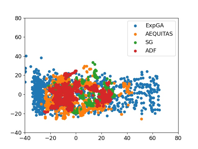
Figure 7. Comparison of the diversity for four approaches.

We also compare the GA to random exploration, keeping seed exploration the same. The results show that without GA, all the SUR values are not higher than 6% and the DSS values are 6 times of those using GA, indicating that GA is significant in generating discriminatory samples. The details can be found on our github.

In summary, even though AEQUITAS is the first approach that proposes a two-phase framework and inspires the following work, its randomly global search scheme leads to detection inefficiency. SG has superior effectiveness than ADF in general and sometimes outperforms ExpGA. However, SG relies on the heavyweight symbolic execution that requires a substantial time consumption when generating testing samples. ADF appears to be a good choice for white-box deep learning models. However, the gradient information required by ADF is often unavailable in most practical scenarios.

Furthermore, we measure the diversity of generated discriminatory samples for the above four approaches. Specifically, we first randomly select 1,000 discriminatory samples on the MLP model for each approach. Then, we translate their features into two dimensions using PCA. As illustrated in Fig. 7, we can observe that the coverage area of ExpGA is larger than others, indicating that the discriminatory samples generated by ExpGA present the most diversity among the four approaches.

Finally, considering the random factors in the above approaches, we use statistical tests to measure their significance of DSS in terms of two metrics, i.e., p-value and effect size (Arcuri and Briand, 2011). To calculate the p-values, we apply the non-parametric Mann-Whitney-Wilcoxon to compare the DSS of ExpGA with those of other three baseline approaches. Then, to calculate the effect size metric, we employ the non-parametric Vargha and Delaney’s $\widehat{A}_{12}$ statistics. The results demonstrate that all the p-values are 0, and all the effect sizes are lower than the standard threshold value, i.e., 0.29, indicating that the DSS of ExpGA is significantly smaller than the others.

Table 6. The performance of ExpGA using CNN model.

Dataset		ExpGA
		TSN	DSN	DSS	SUR
IMDB	gender	44,381	2,477	16.42	5.60%
	country	24,405	357	118.8	1.46%
SST	gender	4,579	105	14.6	2.29%
	country	4,669	252	4.8	5.40%

Table 7. The performance of ExpGA using LR model.

Dataset		ExpGA
		TSN	DSN	DSS	SUR
IMDB	gender	77,898	1,292	13.29	1.66%
	country	17,245	257	46.76	1.49%
SST	gender	10,977	620	2.39	5.65%
	country	4,932	234	4.90	4.74%

Table 8. Comparison results of detecting discriminatory samples between ExpGA and MT-NLP on IMDB dataset.

Dataset	Model	ExpGA				MT-NLP
		TSN	DSN	DSS	SUR	TSN	DSN	DSS	SUR
IMDB gender	CNN	44,381	2,477	16.42	5.60%	174,183	1,111	90.73	0.64%
	LR	77,898	1,292	13.29	1.66%	174,183	1,322	76.25	0.76%

Table 9. Comparison results of detecting discriminatory samples before and after retraining.

Dataset		Sample Added	Normal Sample Testing Accuracy		Discriminatory Sample Testing Percentage		DSS			SUR
			Before	After	Before	After	Before	After	Impr	Before	After	Impr
Cencus	gender	10%	84.65%	84.41%	100%	0.1%	0.03	0.37	12.3x	28.70%	11.14%	61.12%
	age	10%	84.65%	83.30%	100%	3.9%	0.12	0.23	1.9x	67.79%	19.87%	70.69%
	race	10%	84.65%	84.60%	100%	1.7%	0.12	0.17	1.4x	33.41%	22.50%	32.65%
Credit	gender	10%	74.17%	74.22%	100%	2.3%	0.06	0.18	3.0x	23.12%	13.97%	39.57%
	age	10%	74.17%	75.81%	100%	7.8%	0.11	0.15	1.4x	73.44%	53.62%	26.98%
Bank	age	10%	89.52%	89.40%	100%	8.4%	0.13	0.33	2.5x	57.90%	41.65%	28.07%
IMDB	gender	2.58%	87.55%	86.24%	100%	0.67%	16.42	211.48	12.8x	5.60%	0.48%	91.43%
	country	0.72%	87.55%	85.70%	100%	0%	118.8	334.07	2.8x	1.46%	0.45%	69.18%
SST	gender	7.31%	79.50%	78.82%	100%	0%	14.6	107.72	7.4x	2.29%	1.16%	49.35%
	country	1.82%	79.50%	77.70%	100%	5.7%	4.8	576.56	120x	5.40%	0.31%	94.26%

4.3. Performance on Text Datasets

To answer RQ2, we randomly select 1,000 samples from the original datasets as our input. Note that we set the iteration parameter for the text datasets $l$ as 20 to stop our algorithm.

Table 6 and Table 7 list the discriminatory sample detection results by ExpGA using CNN and LR models, respectively. From the results, we can draw two main conclusions.

• The results show that ExpGA can effectively detect discriminatory samples. However, the performance measured by DSS and SUR on text datasets is worse than that on tabular datasets shown in RQ1. The performance difference is due to that the word replacement in ExpGA employs different strategies for text and tabular datasets. On tabular datasets, a word can be replaced by many candidates. On text datasets, a word only can be finitely replaced by its synonyms to retain the syntax and semantic correctness of a sentence after word substitution. As a result, DSN calculated on text datasets is smaller than that on tabular datasets.

• We observe that DSS values on the IMDB dataset are bigger than those on the SST dataset. It indicates that the detection on the former dataset requires a greater time consumption than that on the latter. The average length of samples in the IMDB dataset is ten times larger than that in the SST dataset. The longer the samples, the larger the detection space, leading to a higher time cost in every iteration.

Moreover, we compare the performance of our approach with MT-NLP based on CNN and LR models. Since the source code of MT-NLP is unavailable, we directly use the performance results evaluated by the work of  (Ma et al., [n.d.]). Table 8 presents the comparison results on IMDB dataset with gender protected attribute. Although ExpGA shows smaller TSN than MT-NLP, its DSS value is about five times smaller than MT-NLP, and the SUR value is at least twice larger than MT-NLP.

4.4. Fairness Improvement through Retraining

To answer RQ3, we employ a data augmented method, used in AEQUITAS (Udeshi et al., 2018) and ADF (Zhang et al., 2020), to investigate the model fairness improvement imposed by the discriminatory samples detected by ExpGA. Following the data augmented method, given a target model, we execute ExpGA to generate discriminatory samples from a dataset. A portion of these discriminatory samples are retained in the original dataset, constructing a new dataset. Based on the updated dataset, we retrain the model and re-execute our ExpGA to test the model fairness.

To verify the fairness of retrained model, we randomly select 1,000 discriminatory samples as the ground-truth. Since RQ2 shows that the DSN on text datasets is much smaller than that of tabular datasets, we use half of the generated discriminatory samples for retraining and the remaining for testing.

The Dataset column and Sample Added column in Table 9 list the datasets with the protected attributes, and the percentage of generated discriminatory samples that remained for constructing new datasets in this experiment. On tabular datasets, $10\%\times|original~{}dataset|$ discriminatory samples are reserved for retraining. On text datasets, the percentages are calculated based on the size of generated discriminatory samples.

The Columns 3-12 in Table 9 show experiment results, i.e., the model accuracy and performance of ExpGA before and after retraining models. Normal Sample Testing Accuracy indicates the model accuracy calculated against normal samples in the datasets, and Discriminatory Sample Testing Percentage is the corresponding accuracy against the ground-truth discriminatory samples. DSS and SUR show the efficiency and effectiveness of ExpGA. Impr columns denote the DSS (or SUR) improvements of After DSS (SUR) vs. Before DSS (SUR). These measurements show that:

• The model accuracies of detecting normal samples are nearly unchanged after retraining models on datasets augmented with the discriminatory samples generated by ExpGA. This observation indicates that the data augmented method has little influence on the classification performance of normal samples.

• After retraining, on average, more than 97% of the original discriminatory samples are not biased to new models, indicating that model fairness has been enhanced significantly.

• The Impr of DSS presents that a much longer time is required to detect a discriminatory sample by ExpGA for re-trained models. For example, in SST dataset using country as the protected attribute, after searching about three hours, only 18 discriminatory samples are detected.

• The SUR values drop by an average of 56% (up to 94.26% in SST dataset), indicating the greater difficulty for a successful generation of a discriminatory sample.

5. Threats to Validity

5.1. Threats to Internal Validity

Interpretable Methods: Our ExpGA relies on interpretable methods, such as LIME (Ribeiro et al., 2016) and SHAP (Lundberg and Lee, 2017), to obtain explanation results for an initial seed selection. In practice, it is difficult for interpretable methods to guarantee perfect explanation results. Consequently, the probably missing or mismatching sensitive features might affect our seed sample quality. To mitigate this threat, our future work will explore more interpretable methods.

Retraining to Improve Model Fairness: In RQ3, we test the model fairness using a data augmented method by imposing discriminatory samples detected by ExpGA. Although the model fairness has been improved a lot, we are not claiming that ExpGA radically combs out the model fairness issue. In the future, a considering of the fairness characteristic during data preparation and model training should be a promising exploration direction (d’Alessandro et al., 2017).

5.2. Threats to External Validity

Limited Experiment Datasets: We evaluate ExpGA on five benchmark datasets that are used by baseline approaches. The results demonstrated that ExpGA outperforms baselines on diverse benchmarks, though we cannot conclude that ExpGA would achieve a good performance on other datasets with other protected attributes. Once new datasets are available, we will further verify ExpGA.

Construction of Knowledge Graph: We construct a prior knowledge graph to identify the words related to protected attributes. Currently, this graph only involves a limited number of protected attributes but sufficient for our experimental evaluation. When using ExpGA to test model fairness regarding other protected attributes, the knowledge graph should be extended to express more domains.

6. Related Work

Fairness Testing: Recently, software fairness testing has received much attention. Galhotra et al. (Galhotra et al., 2017) pioneered a fairness test method named THEMIS. THEMIS distinguishes the group discrimination and individual discrimination for software fairness testing. However, the strategy of randomly generating test cases in THEMIS is inefficient. Following the definitions coined by THEMIS, Udeshi et al. (Udeshi et al., 2018) proposed AEQUITAS, achieving a better efficiency by a directional searching scheme. This search scheme makes it difficult for AEQUITAS to cover samples in diverse distributions. Agarwal et al. (Aggarwal et al., 2019) proposed SG based on program symbolic execution. SG uses LIME to generate local perturbation samples to build a decision tree and then analyzes each tree path to generate test inputs. Similar to SG, our ExpGA also leverages the interpretable method LIME. The difference is that ExpGA uses explanation results to identify high-quality seed samples. ADF (Zhang et al., 2020) is a detection method specifically designed for DNN networks. ADF requires gradient information from the model architecture, thus restricting its practical usage. Chakraborty et. al (Chakraborty et al., 2021) thought that data imbalance and improper data label are two main reasons for model biased, thus they proposed Fair-SMOTE to achieve group fairness. Fair-SMOTE first synthetically generates new data points for all the subgroups except the subgroup having the maximum number of data points to solve data imbalance in training data. Then, it find out and remove biased samples in training data to eliminate biased labels. It is worth noting that our work focuses on individual fairness, while Fair-SMOTE focuses on group fairness. Therefore, we do not compare our work with Fair-SMOTE in this paper.

In summary, compared with these approaches, our ExpGA is a lightweight model-agnostic individual fairness testing method, able to handle diverse and large-scale scenarios.

Interpretable Methods: This work is also related to researches related to machine learning interpretable methods. Ribeiro et al. proposed a fast and effective method LIME (Ribeiro et al., 2016) that fits a local decision boundary with a simple linear regression model. The weight of the linear model represents the importance of features. Lundberg and Lee (Lundberg and Lee, 2017) proposed SHAP, generates a set of shap values based on linear functions to represent the coefficients of each feature. Unlike LIME, SHAP defines multiple SHAP kernels as a weight function. At the same time, inspired by game theory, SHAP defines three properties to constrain the fitting process. Guidotti et al. (Guidotti et al., 2018) proposed a rule-based black box model interpretable method called LORE, which first uses genetic algorithms to generate two sample sets with completely different labels. Then, it constructs a decision tree and extracts a set of rules from the tree as a local explanation. Considering that a single linear function cannot fit the highly nonlinear decision boundary well, Guo et al. (Guo et al., 2018) used multiple linear models to approximate the local decision boundary and chose the one with the highest accuracy as interpretation result.

7. Conclusion

This work proposes ExpGA, an explanation-guided method through the GA for software fairness testing. The novelty of ExpGA is the combination of explanation results and GA, thus determining its high efficiency and effectiveness in discriminatory sample detection. ExpGA is also model-agnostic and can handle black-box models in diverse scenarios. The evaluation experiments demonstrate that ExpGA can detect discriminatory samples much faster with a higher success rate than four state-of-the-art methods, both on the text and tabular benchmarks. Augmented with the discriminatory samples generated by ExpGA, the fairness of tested models has a substantial improvement through retraining.

References

- (1)
- Aeq (2018) 2018. AEQUITAS Github Project. https://github.com/sakshiudeshi/Aequitas.
- ADF (2020) 2020. ADF Github Project. https://github.com/pxzhang94/ADF.
- Ban (2021) 2021. Bank Marketing Dataset. https://archive.ics.uci.edu/ml/datasets/Bank+Marketing.
- Cen (2021) 2021. Census Income Dataset. http://archive.ics.uci.edu/ml/datasets/Census+Income.
- Con (2021) 2021. ConceptNet: An open, multilingual knowledge graph. https://conceptnet.io/.
- AI3 (2021) 2021. Fairness 360: Understand and mitigate bias in ML models. https://ai-fairness-360.org/.
- Cre (2021) 2021. German Credit Dataset. https://archive.ics.uci.edu/ml/datasets/statlog+(german+credit+data).
- IMD (2021) 2021. IMDB Dataset. https://www.imdb.com/interfaces/.
- Fai (2021) 2021. ML-fairness-gym: A Tool for Exploring Long-Term Impacts of Machine Learning Systems. https://ai.googleblog.com/2020/02/ml-fairness-gym-tool-for-exploring-long.html.
- GDP (2021) 2021. Principle (a): Lawfulness, fairness and transparency. https://ico.org.uk/for-organisations/guide-to-data-protection/guide-to-the-general-data-protection-regulation-gdpr/principles/lawfulness-fairness-and-transparency/.
- Pro (2021) 2021. The Role of Protected Attributes in AI Fairness. https://www.trustscience.com/blog/the-role-of-protected-attributes-in-ai-fairness.
- SKL (2021) 2021. Scikit-Learn. https://scikit-learn.org/stable/user_guide.html.
- SST (2021) 2021. Stanford Sentiment Treebank Dataset. http://nlpprogress.com/english/sentiment_analysis.html.
- Ten (2021) 2021. TensorFlow. https://github.com/tensorflow/tensorflow.
- Aggarwal et al. (2019) Aniya Aggarwal, Pranay Lohia, Seema Nagar, Kuntal Dey, and Diptikalyan Saha. 2019. Black box fairness testing of machine learning models. In Proc. FSE. 625–635.
- Arcuri and Briand (2011) Andrea Arcuri and Lionel Briand. 2011. A practical guide for using statistical tests to assess randomized algorithms in software engineering. In Proc.ICSE. IEEE, 1–10.
- Brun and Meliou (2018) Yuriy Brun and Alexandra Meliou. 2018. Software fairness. In Proc. FSE. 754–759.
- Buolamwini and Gebru (2018) Joy Buolamwini and Timnit Gebru. 2018. Gender shades: Intersectional accuracy disparities in commercial gender classification. In Proc. FAT. 77–91.
- Chakraborty et al. (2021) Joymallya Chakraborty, Suvodeep Majumder, and Tim Menzies. 2021. Bias in Machine Learning Software: Why? How? What to do? arXiv preprint arXiv:2105.12195 (2021).
- Corbett-Davies and Goel (2018) Sam Corbett-Davies and Sharad Goel. 2018. The measure and mismeasure of fairness: A critical review of fair machine learning. arXiv preprint arXiv:1808.00023 (2018).
- d’Alessandro et al. (2017) Brian d’Alessandro, Cathy O’Neil, and Tom LaGatta. 2017. Conscientious classification: A data scientist’s guide to discrimination-aware classification. Big data 5, 2 (2017), 120–134.
- Fan et al. (2020) Ming Fan, Wenying Wei, Xiaofei Xie, Yang Liu, Xiaohong Guan, and Ting Liu. 2020. Can We Trust Your Explanations? Sanity Checks for Interpreters in Android Malware Analysis. IEEE Transactions on Information Forensics and Security 16 (2020), 838–853.
- Foulds et al. (2020) James R Foulds, Rashidul Islam, Kamrun Naher Keya, and Shimei Pan. 2020. An intersectional definition of fairness. In Proc. ICDE. 1918–1921.
- Galhotra et al. (2017) Sainyam Galhotra, Yuriy Brun, and Alexandra Meliou. 2017. Fairness testing: testing software for discrimination. In Proc. FSE. 498–510.
- Guidotti et al. (2018) Riccardo Guidotti, Anna Monreale, Salvatore Ruggieri, Dino Pedreschi, Franco Turini, and Fosca Giannotti. 2018. Local rule-based explanations of black box decision systems. arXiv preprint arXiv:1805.10820 (2018).
- Guo et al. (2018) Wenbo Guo, Dongliang Mu, Jun Xu, Purui Su, Gang Wang, and Xinyu Xing. 2018. Lemna: Explaining deep learning based security applications. In Proc. CCS. 364–379.
- Lundberg and Lee (2017) Scott M Lundberg and Su-In Lee. 2017. A unified approach to interpreting model predictions. In Proc. NeurIPS. 4765–4774.
- Ma et al. ([n.d.]) Pingchuan Ma, Shuai Wang, and Jin Liu. [n.d.]. Metamorphic testing and certified mitigation of fairness violations in nlp models. In Proc. IJCAI. 458–465.
- Mehrabi et al. (2019) Ninareh Mehrabi, Fred Morstatter, Nripsuta Saxena, Kristina Lerman, and Aram Galstyan. 2019. A survey on bias and fairness in machine learning. arXiv preprint arXiv:1908.09635 (2019).
- Mishra et al. (2019) Deepti Bala Mishra, Rajashree Mishra, Arup Abhinna Acharya, and Kedar Nath Das. 2019. Test data generation for mutation testing using genetic algorithm. In Soft Computing for Problem Solving. 857–867.
- Mitchell et al. (2018) Shira Mitchell, Eric Potash, Solon Barocas, Alexander D’Amour, and Kristian Lum. 2018. Prediction-based decisions and fairness: A catalogue of choices, assumptions, and definitions. arXiv preprint arXiv:1811.07867 (2018).
- Pedreshi et al. ([n.d.]) Dino Pedreshi, Salvatore Ruggieri, and Franco Turini. [n.d.]. Discrimination-aware data mining. In Proc. KDD. 560–568.
- Pennington et al. (2014) Jeffrey Pennington, Richard Socher, and Christopher D Manning. 2014. Glove: Global vectors for word representation. In Proc. EMNLP. 1532–1543.
- Ribeiro et al. (2016) Marco Tulio Ribeiro, Sameer Singh, and Carlos Guestrin. 2016. why should i trust you?: Explaining the predictions of any classifier. In Proc. KDD. 1135–1144.
- Ribeiro et al. (2018) Marco Tulio Ribeiro, Sameer Singh, and Carlos Guestrin. 2018. Anchors: High-precision model-agnostic explanations. In Proc. AAAI. 1527–1535.
- Saxena (2019) Nripsuta Ani Saxena. 2019. Perceptions of Fairness. In Proc. AIES. 537–538.
- Sharma et al. (2016) Akshat Sharma, Rishon Patani, and Ashish Aggarwal. 2016. Software testing using genetic algorithms. International Journal of Computer Science & Engineering Survey 7, 2 (2016), 21–33.
- Tatman (2017) Rachael Tatman. 2017. Gender and dialect bias in YouTube automatic captions. In Proc. EthNLP@EACL. 53–59.
- Tramer et al. (2017) Florian Tramer, Vaggelis Atlidakis, Roxana Geambasu, Daniel Hsu, Jean-Pierre Hubaux, Mathias Humbert, Ari Juels, and Huang Lin. 2017. Fairtest: Discovering unwarranted associations in data-driven applications. In Proc. EuroS&P. 401–416.
- Udeshi et al. (2018) Sakshi Udeshi, Pryanshu Arora, and Sudipta Chattopadhyay. 2018. Automated directed fairness testing. In Proc. ASE. 98–108.
- Warnecke et al. (2020) Alexander Warnecke, Daniel Arp, Christian Wressnegger, and Konrad Rieck. 2020. Evaluating explanation methods for deep learning in security. In Proc. EuroS&P. 158–174.
- Zhang et al. (2020) Peixin Zhang, Jingyi Wang, Jun Sun, Guoliang Dong, Xinyu Wang, Xingen Wang, Jin Song Dong, and Ting Dai. 2020. White-box fairness testing through adversarial sampling. In Proc. ICSE. 949–960.
- Zhang and Tao (2017) Ridong Zhang and Jili Tao. 2017. A nonlinear fuzzy neural network modeling approach using an improved genetic algorithm. IEEE Transactions on Industrial Electronics 65, 7 (2017), 5882–5892.