Out-of-equilibrium dynamics arising from slow round-trip variations of
Hamiltonian parameters across quantum and classical critical points

Abstract

We address the out-of-equilibrium dynamics of many-body systems subject to time-dependent round-trip protocols across quantum and classical (thermal) phase transitions. They are realized by slowly changing one relevant parameter $w$ across its critical point $w_{c}=0$, linearly in time with a large time scale $t_{s}$, from $w_{i}<0$ to $w_{f}>0$ and then back to $w_{i}<0$, thus entailing multiple passages through the critical point. Analogously to the one-way Kibble-Zurek protocols across a critical point, round-trip protocols develop dynamic scaling behaviors at both classical and quantum transitions, put forward within renormalization-group frameworks. The scaling scenario is analyzed within some paradigmatic models undergoing quantum and classical transitions belonging to the two-dimensional Ising universality class, such as one-dimensional quantum Ising models and fermionic wires, and two-dimensional classical Ising models (supplemented with a purely relaxational dynamics). While the dynamic scaling frameworks are similar for classical and quantum systems, substantial differences emerge due to the different nature of their dynamics, which is purely relaxational for classical systems (implying thermalization in the large-time limit at fixed model parameters), and unitary in the case of quantum systems. In particular, when the critical point separates two gapped (short-ranged) phases and the extreme value $w_{f}>0$ is kept fixed in the large-$t_{s}$ limit of the round-trip protocol, we observe hysteresis-like scenarios in classical systems, while quantum systems do not apparently develop a sufficiently robust scaling limit along the return way, due to the presence of rapidly oscillating relative phases among the relevant quantum states.

I Introduction

Many-body systems generally develops out-of-equilibrium phenomena when they are driven across phase transitions, due to the fact that large-scale critical modes do not equilibrate, even when the time scale $t_{s}$ of the variation of the system parameters is taken very large. Out-of-equilibrium dynamic phenomena at phase transitions, such as hysteresis and coarsening, Kibble-Zurek (KZ) defect production, aging, etc., have been addressed in a variety of contexts, both experimentally and theoretically, at classical and quantum phase transitions (see, e.g., Refs. Kibble-76 ; Kibble-80 ; Binder-87 ; CDTY-91 ; BCSS-94 ; Bray-94 ; Zurek-96 ; BBFGP-96 ; CG-05 ; BDS-06 ; WNSBD-08 ; Dziarmaga-10 ; PSSV-11 ; Ulm-etal-13 ; Pyka-etal-13 ; NGSH-15 ; Biroli-16 ; Trenkwalder-etal-16 ; RV-21 and references therein). Out-of-equilibrium scaling behaviors generally emerge when slowly crossing a critical point, i.e. in the large-$t_{s}$ limit. They depend on the nature of the classical or quantum transition, its universality class, and the type of critical dynamics in classical systems, see e.g. Refs. Kibble-80 ; Zurek-85 ; Zurek-96 ; Polkovnikov-05 ; ZDZ-05 ; Dziarmaga-05 ; PG-08 ; Dziarmaga-10 ; DGP-10 ; GZHF-10 ; PSSV-11 ; CEGS-12 ; Dutta-etal-book ; PV-16 ; PRV-18-loc ; PRV-18 ; RV-19-de ; RV-20 ; RV-21 . Therefore, slow (quasi-adiabatic) passages through critical points allow us to probe the universal features of the long-range modes emerging at thermal and quantum critical phenomena.

In both classical and quantum contexts, we consider many-body systems whose Hamiltonian can be written as

$$H(t)\equiv H[w(t)]=H_{c}+w(t)\,H_{p}\,,$$ (1)

where $w(t)$ is a time-dependent Hamiltonian parameter, while $H_{c}$ and $H_{p}$ do not depend on time. $H_{c}$ is supposed to be a critical Hamiltonian at its transition point, which may be a quantum continuous transition driven by quantum fluctuations, or a classical continuous transition driven by thermal fluctuations. $H_{p}$ represents a nontrivial relevant perturbation. In particular, within quantum many-body models, one generally assumes that $[H_{c},H_{p}]\neq 0$. The tunable parameter $w$ controls the strength of the coupling with the perturbation $H_{p}$, and is taken as a relevant parameter driving the continuous transition. Therefore $w_{c}=0$ corresponds to the transition point. The scaling properties of the out-of-equilibrium dynamics across phase transitions can be probed by considering time-dependent protocols where one of the relevant parameters, such as $w(t)$, is slowly changed across the transition point $w_{c}=0$, linearly in time with a large time scale $t_{s}$.

Across a phase transition, the growth of an out-of-equilibrium dynamics is inevitable in the thermodynamic limit, even for very slow changes of the parameter $w$, because large-scale modes are unable to equilibrate the long-distance critical correlations emerging at the transition point, even in the limit of large time scales of the variations. As a consequence, when starting from equilibrium states at the initial value $w_{i}$, the system cannot pass through equilibrium states associated with the values of $w(t)$ across the transition point, thus departing from an adiabatic dynamics. Such a departure from equilibrium develops peculiar out-of-equilibrium dynamic scaling phenomena in the limit of large time scale $t_{s}$ of the time variation of $w(t)$. A related issue is the so-called KZ problem, i.e. the scaling behavior of the amount of final defects after slow passages through continuous transitions, from the disorder phase to the order phase Kibble-76 ; Kibble-80 ; Zurek-85 ; Zurek-96 ; ZDZ-05 ; Polkovnikov-05 ; Dziarmaga-05 ; PG-08 ; Dziarmaga-10 ; Dutta-etal-book ; PSSV-11 ; CEGS-12 ; RV-21 ; Damski-05 ; USF-07 ; USF-10 ; NDP-13 ; DZ-14 ; RDZ-19 ; RMAKVE-21 . The general features of the KZ dynamic scaling, and in particular the KZ predictions for the abundance of residual defects, have been confirmed by several analytical and numerical studies, see, e.g., Refs. Dziarmaga-10 ; Dutta-etal-book ; PSSV-11 ; CEGS-12 ; NDP-13 ; RV-21 and citing references, and by experiments for various physically interesting systems, see, e.g., Refs. DRGA-99 ; MMARK-06 ; SHLVS-06 ; WNSBD-08 ; CWBD-11 ; Griffin-etal-12 ; Ulm-etal-13 ; Pyka-etal-13 ; LDSDF-13 ; Braun-etal-15 ; Chomaz-etal-15 ; NGSH-15 ; Cui-etal-16 ; Gong-etal-16 ; Anquez-etal-16 ; CFC-16 ; Keesling-etal-19 .

The out-of-equilibrium scaling behaviors of many-body systems subject to slow passages across classical and quantum critical points present notable analogies. They can be discussed within a unified renormalization-group (RG) framework, like the equilibrium scaling behaviors that can be related by the quantum to classical mapping, see e.g. Refs. Sachdev-book ; RV-21 . However, we should recall that, while quantum systems are ruled by the unitary dynamics of quantum mechanics, the out-of-equilibrium scaling behavior of classical systems depend also on the particular choice of dynamics, whether it is purely relaxational or it implies conserved quantities, which gives generally rise to different dynamic features HH-77 ; Ma-book ; FM-06 .

In this paper we address the effects of slow round-trip variations of the Hamiltonian parameter $w(t)$ in Eq. (1), entailing multiple crossings of quantum and thermal transitions. More precisely, we consider round-trip protocols where the system starts at the equilibrium condition (ground state in quantum systems) associated with the initial value $w_{i}=w(t_{i})<0$, then the out-of-equilibrium dynamics is driven by linear changes of $w(t)$ up to $w_{f}>0$, thus crossing the transition point $w_{c}=0$, and then by changing it back to the original value $w_{i}<0$, again linearly in time, which implies a further crossing of the transition point. The time scale $t_{s}$ of the variations of $w(t)$ is unique, and the slow-crossing regime is realized in the large-$t_{s}$ limit.

We address these issues within classical (see e.g. Ref. Cardy-book ) and quantum (see e.g. Ref. Sachdev-book ) continuous transitions, characterized by emerging long-range correlations. We exploit unified RG frameworks WK-74 ; Fisher-74 ; Wegner-76 ; Ma-book ; Parisi-book ; PV-02 ; Cardy-book ; SGCS-97 ; Sachdev-book ; RV-21 , which allow us to derive general dynamic scaling behaviors at both classical and quantum transitions, in the limits of large time scale $t_{s}$ of the round-trip KZ protocol and large size $L$ of the model, using standard RG arguments. For this purpose, we extend the dynamic RG framework already applied to standard one-way KZ protocols, see e.g. Refs. CEGS-12 ; RV-21 and references therein.

In this exploratory study of slow round-trip protocols across continuous transitions, we restrict ourselves to transitions between gapped phases showing only short-ranged correlations, to avoid the complications arising from the effects of gapless modes in the ordered phases. This is somehow different from the standard KZ protocols leading to the KZ problem, in which, starting from a disordered phase, the system is driven to an ordered phases characterized by long-range correlations, where further important dynamic effects may set in at large time, such as coarsening phenomena or massless Goldstone excitations, see e.g. Refs. CEGS-12 ; PV-16 .

In our study we consider some paradigmatic many-body systems undergoing quantum and classical transitions belonging to the two-dimensional (2D) Ising universality class:

(i) Quantum one-dimensional (1D) Ising models with an external time-dependent longitudinal field;

(ii) Quantum Kitaev fermionic wires with a time-dependent chemical potential;

(iii) Classical 2D lattice Ising models undergoing a finite-temperature transition, supplemented with a purely relaxational dynamics driven by an external time-dependent magnetic field.

In all cases we consider time-dependent protocols with round-trip variations of the Hamiltonian parameter corresponding to $w(t)$ in Eq. (1), crossing twice the critical point separating classical or quantum phases with finite correlation lengths, when $|w(t)|>0$ in Eq. (1).

As we shall see, the analogy of the scaling behaviors emerging from standard one-way KZ protocols at classical and quantum transitions is only partially extended to round-trip KZ protocols. Indeed substantial differences emerge, in particular when the extreme value $w_{f}>0$ at the return point (where $w(t)$ stops increasing and starts decreasing) is kept fixed and finite in the large-$t_{s}$ dynamic scaling limit of the round-trip protocol. On the one hand, classical systems show well-defined scaling phenomena, developing hysteresis-like scenarios; this is essentially related to the fact that the purely relaxational stochastic dynamics leads eventually to thermalization in the large-time limit when keeping the model parameters fixed Parisi-book . On the other hand, in quantum systems the observation of scaling behaviors along the return way turns out to be more problematic, due to the persistence of rapidly oscillating relative phases between the relevant quantum states, which make the return way extremely sensitive to the parameters of the protocol, such as the extreme value $w_{f}$ and the size of the system. This is essentially related to the quantum unitary nature of the dynamics. Indeed we observe some notable similarities with the behavior of quantum two-level models subject to round-trip protocols, related to the well-known Landau-Zener-Stückelberg problem LZeff ; VG-96 ; SAN-10 ; ISN-22 . Even in this apparently simple case some features of the behavior along the return way turn out to be extremely sensitive to the parameters of the round-trip protocol.

The paper is organized as follows. In Sec. II we introduce the above-mentioned quantum and classical models that develop critical behaviors belonging to the 2D Ising universality class. In Sec. III we describe the one-way and round-trip KZ protocols that we consider, across thermal and quantum transitions. Sec. IV reports the observables that we use to monitor the dynamic evolution along the KZ protocols in the various models considered. Sec. V summarizes the dynamic scaling theory associated with one-way KZ protocols, within RG frameworks which apply to both classical and quantum transitions. In Sec. VI we extend the dynamic scaling theory to round-trip KZ protocols, emphasizing the possible differences between classical and quantum behaviors. Sec. VII reports the numerical analyses that support, and further characterize, the predicted dynamic scaling behaviors, showing also substantial differences between classical and quantum round-trip KZ protocols. Finally, in Sec. VIII we summarize and draw our conclusions. The App. A analyzes analogous round-trip protocols within a two-level quantum model with time-dependent Hamiltonian parameters (similar to that used for the so-called Landau-Zener-Stückelberg problem), which turns out to be useful to interpret the results obtained for the quantum many-body systems.

II The models

II.1 Quantum many-body systems

As a paradigmatic quantum many-body system we consider the 1D quantum Ising models, described by the Hamiltonian

$$H_{qI}(g,h)=-J\sum_{x=1}^{L}\sigma^{(1)}_{x\phantom{1}}\sigma^{(1)}_{x+1}-g\sum_{x=1}^{L}\sigma^{(3)}_{x}-h\sum_{x=1}^{L}\sigma^{(1)}_{x}\,,\quad$$ (2)

where $L$ is the system size, $\sigma^{(k)}_{x}$ are the Pauli matrices on the $x^{\rm th}$ site ($k=1,2,3$ labels the three spatial directions). In the following we consider quantum Ising systems with periodic boundary conditions (PBC), obtained by requiring $\sigma^{(k)}_{L+1}=\sigma^{(k)}_{1}$.

We recall that the quantum Ising model (2) develops a quantum critical behavior at $g=g_{c}=J$ and $h=0$, belonging to the 2D Ising universality class, see e.g. Ref. Sachdev-book . The model is always gapped for $h\neq 0$. The relevant parameters $r\equiv g-g_{c}$ and $h$ are respectively associated with even and odd RG perturbations at the Ising fixed point. Their RG dimensions are respectively $y_{r}=1/\nu=1$ and $y_{h}=15/8$, so that the length scale $\xi$ of the critical modes behaves as $\xi\sim|g-g_{c}|^{-1/y_{r}}$ for $h=0$, and $\xi\sim|g-g_{c}|^{-1/y_{h}}$ at $g=g_{c}$. The dynamic exponent $z$, controlling the vanishing of the gap $\Delta\sim\xi^{-z}$ at the transition point, is given by $z=1$. Moreover, we recall that the RG dimension of the order-parameter field, associated with the longitudinal operators $\sigma_{x}^{(1)}$, is given by $y_{l}=d+z-y_{h}=1/8$, while that associated with the transverse operator $\sigma_{x}^{(3)}$ is given by $y_{t}=d+z-y_{r}=1$. In the following we assume ferromagnetic nearest-neighbour interactions with $J=1$, thus $g_{c}=J=1$.

To achieve round-trip protocols between gapped phases, without degeneration of the lowest quantum states, we consider Ising chains with PBC at $g=g_{c}$ driven by a time-dependent longitudinal field $h(t)$. Therefore, comparing with Eq. (1), we identify

$$H_{c}=H_{qI}(g_{c},0)\,,\quad w(t)=h(t)\,,\quad H_{p}=-\sum_{x}\sigma^{(1)}_{x}\,.$$ (3)

The quantum Ising Hamiltonian $H_{qI}(g,0)$ for vanishing longitudinal field $h$ can be mapped into a quadratic model of spinless fermions through a Jordan-Wigner transformation LSM-61 ; Katsura-62 , obtaining the so-called quantum Kitaev wire: Kitaev-01

$$H_{K}(\mu)=-\sum_{x}\big{(}c_{x}^{\dagger}c_{x+1}+c_{x}^{\dagger}c_{x+1}^{\dagger}+{\rm h.c.}\big{)}-\mu\sum_{x}n_{x}\,,$$ (4)

where $c_{x}^{(\dagger)}$ is the fermionic annihilation (creation) operator on site $x$ of the wire, $n_{x}\equiv c_{x}^{\dagger}c_{x}$ is the corresponding number operator, and $\mu=-2g$. The Kitaev model undergoes a continuous quantum transition at $\mu_{c}=-2g_{c}=-2$. Of course, it belongs to the 2D Ising universality class as well, so that $y_{\mu}=y_{r}=1/\nu=1$ (there is no an analogue of the longitudinal field $h$ of the spin formulation (2) within the above fermionic representation). At the Ising transition the fermionic operators $c_{x}$ and the particle density operator $n_{x}$ acquire the RG dimensions $y_{c}=1/2$ and $y_{n}=1$, respectively.

Although the bulk behaviors of the Ising and Kitaev models in the infinite-volume limit (and thus their phase diagram) are analogous, some features of finite-size systems may significantly differ. As a matter of fact, the nonlocal Jordan-Wigner transformation of the Ising chain with PBC does not simply map into the fermionic model (4) with definte boundary conditions. Indeed further considerations apply Katsura-62 ; Pfeuty-70 , leading to a less straightforward correspondence, which also depends on the parity of the particle-number eigenvalue.

The Kitaev quantum wire with antiperiodic boundary conditions (ABC), obtained by requiring that $c_{L+1}=-c_{1}$, turns out to be gapped in both phases separated by the quantum transition at $\mu_{c}=-2$. Indeed, it does not exhibit the lowest-state degeneracy of the ordered phase of the quantum Ising chain (namely, the exponential suppression of the gap with increasing $L$). The reason for such substantial difference resides in the fact that the Hilbert space of the former is restricted with respect to that of the latter, so that it is not possible to restore the competition between the two vacua belonging to the symmetric/antisymmetric sectors of the Ising model Katsura-62 ; Kitaev-01 ; CPV-14 ; RV-21 . Therefore, a continuous quantum transition between gapped phases is also realized within the Kitaev wire with ABC, by choosing

$$H_{c}=H_{K}(\mu_{c})\,,\quad w(t)=\mu(t)-\mu_{c}\,,\quad H_{p}=-\sum_{x}n_{x}\,.\;\;$$ (5)

II.2 Classical Ising model

As a classical paradigmatic model undergoing a finite-temperature continuous transition, we consider the 2D Ising model, defined on a square lattice by the partition function

$$Z=\sum_{\{s_{\bm{x}}\}}e^{-\beta H_{cI}}\,,\qquad\beta=1/T\,,$$ (6)

$$H_{cI}(J,h)=-J\sum_{\langle{\bm{x}}{\bm{y}}\rangle}s_{\bm{x}}s_{\bm{y}}-h\sum_{\bm{x}}s_{\bm{x}}\,,$$ (7)

where ${\bm{x}}$ are the sites of the lattice, ${\langle{\bm{x}}{\bm{y}}\rangle}$ indicates the nearest-neighbour sites of the lattice, $s_{\bm{x}}=\pm 1$ are classical spin variables, and $h$ is an external homogenous magnetic field (we use the same symbol of the external longitudinal field of the quantum ising model (2), but this should not lead to confusion). We consider systems with PBC. We again set $J=1$.

The square-lattice Ising model (7) undergoes a thermal continuous transition at $h=0$ and $T_{c}=2/\ln(\sqrt{2}+1)$ Onsager-44 . The critical behavior belongs to the same universality class of the 1D quantum Ising model. Therefore, it is characterized by the critical exponents $\nu=1$ and $\eta=1/4$. They are related to the RG dimension $y_{t}$ associated with the even temperature parameter by $y_{t}=1/\nu=1$, and to that associated with the odd external field $h$ by $y_{h}=2-\eta/2=15/8$, see e.g. Ref. PV-02 .

Since we are going to discuss dynamic behaviors, we must also define the type of dynamics driving the time evolution of the system. We consider a purely relaxational dynamics (also known as model A of critical dynamics HH-77 ; Ma-book ), which can be realized by stochastic Langevin equations, or just Metropolis updatings in Monte Carlo simulations Metropolis:1953am . The corresponding dynamic exponent $z$ has been accurately estimated by numerical studies, obtaining $z\approx 2.167$ with a relative precision that is apparently better than one per mille. Indeed, some of the most recent estimates of the dynamic exponent $z$ for purely relaxational dynamics are $z=2.1667(5)$ from NB-00 , $z=2.168(5)$ from WH-97 , $z=2.1665(12)$ from NB-96 , $z=2.172(6)$ from G-95 , $z=2.170(6)$ from Ref. CV-11 , which have been obtained by numerical analyses based on Monte Carlo simulations in equilibrium conditions. In the following we use the estimate $z=2.167(1)$.

One may consider time-dependent KZ protocols also in this classical context, supplementing the partition function (6) defining the classical Ising model with the purely relaxational dynamics. Analogously to the quantum case, cf. Eq. (3), we consider 2D Ising models with PBC at $T_{c}$ driven by a time-dependent magnetic field $h(t)$. Therefore, we identify

$$H_{c}=H_{cI}(1,0)\,,\qquad \beta=\beta_{c}={\ln(\sqrt{2}+1)\over 2}\,,$$

$$w(t)=h(t)\,,\qquad H_{p}=-\sum_{\bm{x}}s_{\bm{x}}\,.$$

III One-way and round-trip KZ protocols across transition points

In the following we assume the general Hamiltonian (1), which represents the three models presented in Sec. II with the identifications in Eqs. (3), (5), and (II.2).

III.1 One-way KZ protocols

KZ-like protocols have been largely employed to investigate the dynamics of critical systems, at quantum transitions when the many-body system is subject to unitary time evolutions, and at classical (thermal) transitions considering, for example, a purely relaxational dynamics that can be implemented by standard Langevin equations HH-77 .

III.1.1 Quantum KZ protocols

In the case of quantum many-body systems, quasi-adiabatic passages through the continuous quantum transition are obtained by slowly varying $w$ across $w_{c}=0$, following, e.g., the standard KZ procedure:

(i) One starts from the ground state of the many-body system at $w_{i}<0$, that is $|\Psi(t=0)\rangle\equiv|\Psi_{0}(w_{i})\rangle$.

(ii) Then the out-of-equilibrium unitary dynamics, ruled by the Schrödinger equation

$${{\rm d}\,|\Psi(t)\rangle\over{\rm d}t}=-i\,\hat{H}[w(t)]\,|\Psi(t)\rangle\,,$$ (9)

arises from a linear time dependence of the Hamiltonian parameter $w(t)$, such as

$$w(t)=t/t_{s}\,,$$ (10)

up to a final value $w_{f}>0$. Therefore the KZ protocol starts at time $t_{i}=t_{s}\,w_{i}<0$ and stops at $t_{f}=t_{s}\,w_{f}>0$. The parameter $t_{s}$ denotes the time scale of the slow variations of the Hamiltonian parameter $w$.

Across a continuous transition, the growth of an out-of-equilibrium dynamics is inevitable in the thermodynamic limit, even for very slow changes of the parameter $w$, because large-scale modes are unable to equilibrate as the system changes phase. Indeed, when starting from the ground state associated with the initial value $w_{i}$, the system cannot pass adiabatically through the ground states associated with $w(t)$ across the transition point (in the infinite volume limit), thus departing from an adiabatic dynamics. Note that, in the quantum cases that we consider, cf. Eqs. (3) and (5), the slow variation of the longitudinal field $w$ brings the system from a gapped condition at $w_{i}<0$ to another gapped condition for $w_{f}>0$. This somehow differs from the standard situation of the KZ problem related to the defect production going from disorder to order phases, see e.g. Refs. Kibble-76 ; Kibble-80 ; Zurek-85 ; Zurek-96 ; ZDZ-05 ; Polkovnikov-05 ; Dziarmaga-05 ; PG-08 ; Dziarmaga-10 ; Dutta-etal-book ; CEGS-12 ; PSSV-11 ; Damski-05 ; USF-07 ; USF-10 ; NDP-13 ; DZ-14 .

III.1.2 Classical KZ protocols

In the case of many-body systems at classical transitions, one can again assume that slow passages through the continuous transition are obtained by slowly varying $w$ across $w_{c}=0$, following the classical KZ procedure:

(i) One starts from an equilibrium thermalized configuration at $w_{i}<0$.

(ii) Then the out-equilibrium classical dynamics, ruled by the relaxational Langevin equation HH-77 , or a standard Metropolis upgrading Metropolis:1953am of lattice configurations, arises from linear changing of the parameter $w(t)$, as $w(t)=t/t_{s}$, up to a final value $w_{f}>0$. In the case of Metropolis-like dynamics, this can be achieved by incrementing the time by one unity after one global sweep of the lattice variables (Metropolis upgrading of all lattice spin variables). Again the KZ protocol starts at time $t_{i}=t_{s}\,w_{i}<0$ and stops at $t_{f}=t_{s}\,w_{f}>0$.

Since the above protocol involves a stochastic relaxational process, results are obtained by averaging over an ensemble of trajectories (starting from an ensenble of thermalized configurations at $w_{i}$), obtained following the above protocol.

We remark again that the classical out-of-equilibrium phenomena associated with the above protocol occurs between two phases, for $w<0$ and $w>0$, with short-ranged correlations. This is again different from standard classical protocols associated with the KZ problem, in which one passes from a disordered to an ordered phase characterized by long-range correlations, where further important dynamic effects may set in, in particular when the global symmetry is preserved by the KZ protocol and its initial state, such as coarsening phenomena or massless Goldstone excitations, see e.g. Ref. CEGS-12 .

III.2 Round-trip KZ protocols

We now consider round-trip protocols in which the Hamiltonian parameter $w(t)$ varies linearly from $w_{i}<0$ to $w_{f}>0$, which is analogous to the one-way KZ protocol, and then it returns back to the original value, crossing twice the transition point. In the case of quantum systems the round-trip KZ protocol follows the steps:

(i) One starts at $t=t_{i}$ from the ground state of the many-body system at $w_{i}<0$, given by $|\Psi(t_{i})\rangle\equiv|\Psi_{0}(w_{i})\rangle$.

(ii) The out-equilibrium unitary dynamics, ruled by the Schrödinger equation (9), is driven by linearly increasing $w(t)$: as $w(t)=t/t_{s}$ from $w_{i}<0$ (at time $t_{i}=w_{i}t_{s}<0$) to $w_{f}>0$ (at time $t_{f}=w_{f}t_{s}>0$).

(iii) Then, for $t>t_{f}$ the dynamics is ruled by the Schrödinger equation (9) with an external field $w(t)$ that decreases linearly with the same time scale $t_{s}$, from $w_{f}>0$ to the original value $w_{i}<0$, closing the cycle.

To simplify the protocol, reducing its number of parameters, we consider a symmetric round-trip KZ protocol (an extension of the later results to the most general case is straightforward) in which we fix

$$w_{\star}=w_{f}=-w_{i}\,,$$ (11)

and write the time dependence of $w(t)$ as

$$w(t)={{\cal T}(t)\over t_{s}}\quad{\rm for}\;\;t_{i}=-t_{\star}\leq t\leq 3t_{\star}\,,$$ (12)

where

$${\cal T}(t)=t_{\star}-|t-t_{\star}|$$ (13)

is the triangular function going linearly from ${\cal T}(-t_{\star})=-t_{\star}$ to ${\cal T}(t_{\star})=t_{\star}$, and then back to ${\cal T}(3t_{\star})=-t_{\star}$. The parameter $t_{s}$ represents the time scale of the variation. The parameter $t_{\star}>0$ controls the extension, i.e. the starting and final times, of the protocols, from $t_{i}=-t_{\star}$ to $t_{f}=3t_{\star}$, and also the interval of variation of $w(t)$, from $w(t_{i})=-t_{\star}/t_{s}$ to $w(t_{\star})=t_{\star}/t_{s}$.

Analogously to the quantum case, we extend the one-way KZ protocol for classical systems to symmetric round-trip KZ protocols, by taking the time-dependent parameter $w(t)$ as in Eq. (12), with the same definitions.

We finally mention that similar cyclic protocols have been also considered in various contexts and phase transitions, see e.g. Refs. PV-16 ; HZFKXJD-11 ; GAQRJ-16 ; ONL-18 ; PYLNL-20 ; BA-20 , in particular at first-order phase transitions to show the emergence of hysteresis phenomena Binder-87 . As we shall see, round-trip KZ protocols of classical systems will also lead to the emergence of a scaling hysteresis-like scenarios, however their nature and scaling propeties are substantially different from that arising at first-order transitions. In this paper we will not pursue hysteresis issues at first-order classical and quantum transitions; however, they may be worth further investigation, as we will mention in the conclusive section.

IV Observables to monitor the out-of-equilibrium dynamics

IV.1 Quantum case

The resulting out-of-equilibrium evolution of quantum many-body systems can be investigated by monitoring observables and correlations at fixed time. To characterize the departure from adiabaticity along the slow dynamic across the continuous transition, we monitor the adiabaticity function

$$A(t)=|\langle\,\Psi_{0}[w(t)]\,|\,\Psi(t)\,\rangle|\,,$$ (14)

where $|\,\Psi_{0}[w(t)]\,\rangle$ is the ground state of the Hamiltonian $H[w(t)]$, i.e. at instantaneous values of $w(t)$, while $|\,\Psi(t)\,\rangle$ is the actual time-dependent state evolving according to the Schrödinger equation (9).

The adiabaticity function measures the overlap of the time-dependent state with the corresponding ground state of the Hamiltonian at the same $w(t)$. Of course, the adiabaticity function for an adiabatic evolution takes the value $A(t)=1$ at any time. Since the KZ protocol starts from the ground state associated with $w_{i}=w(t_{i})$, we have $A(t_{i})=1$ initially. In general protocols crossing transition points, $A(t)$ is expected to depart from the initial value $A(t_{i})=1$, due to the impossibility of the system to adiabatically follow the changes of the function $w(t)$ across its critical value $w=0$. Note however that this is strictly true in the infinite-volume limit. In systems of finite size $L$, there is always a sufficiently large time scale $t_{s}$, so that the system can evolve adiabatically, essentially because finite-size systems are strictly gapped, although the gap $\Delta$ at the continuous quantum transition gets suppressed as $\Delta\sim L^{-z}$. The interplay between the size $L$ and the time scale $t_{s}$ gives rise to nontrivial out-of-equilibrium scaling behaviors, which can be studied within finite-size scaling (FSS) frameworks RV-21 ; RV-20 .

Another general observable is related to the surplus energy of the system with respect to its instantaneous ground state at the given $w(t)$, i.e.

$$E_{s}(t)=\langle\Psi(t)|\,H\,|\Psi(t)\rangle-\langle\Psi_{0}[w(t)]|\,H\,|\Psi_{0}[w(t)]\rangle\,.$$ (15)

Since the protocols considered start from a ground state at $t_{i}$, the surplus energy $E_{s}(t)$ vanishes along adiabatic evolutions, while nonzero values $E_{s}(t)>0$ are related to the degree of out-of-equilibrium of the dynamics across the transition.

To monitor the out-of-equilibrium dynamics in the case of Ising models in the presence of a time-dependent longitudinal field $w(t)$, one may consider the evolution of the local and global average magnetization

$$m_{x}(t)\equiv\langle\Psi(t)|\,\sigma_{x}^{(1)}\,|\Psi(t)\rangle\,,\;\;\;M(t)\equiv{1\over L}\sum_{x}m_{x}(t)\,,$$ (16)

as well as the fixed-time correlation function of the order-parameter operator and its space integral,

$$G(t,x,y)\equiv\langle\Psi(t)|\,\sigma_{x}^{(1)}\,\sigma_{y}^{(1)}\,|\Psi(t)\rangle\,.$$ (17)

Taking into account the translation invariance due to the absence of boundaries (such as the cases with PBC or ABC), we trivially have $m_{x}(t)=M(t)$ and $G(t,x,y)\equiv G(t,x-y)$. We also consider the transverse magnetization

$$N(t)\equiv{1\over L}\sum_{x}\langle\Psi(t)|\,\sigma_{x}^{(3)}\,|\Psi(t)\rangle\,,$$ (18)

and the related subtracted quantity

$$N_{s}(t)=N(t)-N_{c}\,,$$ (19)

where $N_{c}$ is the ground-state transverse magnetization at the critical point, i.e. Pfeuty-70

$$N_{c}=\lim_{L\to\infty}\langle\Psi_{0},w=0|\sigma_{x}^{(3)}|\Psi_{0},w=0\rangle={2\over\pi}\,.$$ (20)

In the case of the Kitaev model with ABC subject to a time-dependent chemical potential, one may consider the particle density, and in particular the subtracted definition

$$\rho_{s}(t)\equiv\langle\Psi(t)|\,n_{x}\,|\Psi(t)\rangle-\rho_{c}\,,$$ (21)

which is independent of $x$ due to translation invariance, and, for convenience, we have subtracted its known critical ground-state value in the infinite volume limit, which is given by Pfeuty-70 $\rho_{c}=(\pi-2)/(2\pi)=0.18169011...$. One may also consider fermionic correlation functions, such as

$$C(x,t) \equiv \langle\Psi(t)|\,c_{j}^{\dagger}c_{j+x}+c_{j+x}^{\dagger}c_{j}\,|\Psi(t)\rangle\,,$$ (22)

where $j,x\in[1,L/2]$, we have taken into account the translation invariance of systems with ABC.

IV.2 Classical case

In the case of the classical 2D Ising systems we consider the magnetization

$$m_{\bm{x}}(t)\equiv\langle s_{\bm{x}}\rangle_{t}\,,\;\;\;M(t)\equiv{1\over L^{2}}\sum_{\bm{x}}m_{\bm{x}}(t)\,,$$ (23)

as well as the fixed-time correlation function of the order-parameter operator and its space integral,

$$G(t,{\bm{x}},{\bm{y}})\equiv\langle s_{\bm{x}}\,s_{\bm{y}}\,\rangle_{t}\,.$$ (24)

The symbol $\langle\;\rangle_{t}$ indicates the average over trajectories at time $t$. Taking into account the translation invariance due to the absence of boundaries (such as the cases with PBC), we trivially have $m_{\bm{x}}(t)=M(t)$ and $G(t,{\bm{x}},{\bm{y}})=G(t,{\bm{x}}-{\bm{y}})$.

V Dynamic scaling along the one-way KZ protocol

In this section we outline the main features of the dynamic scaling behavior that is expected to emerge at the one-way KZ protocol of the models introduced in the previous sections, driven by the time dependent $w(t)=t/t_{s}$, starting from equilibrium conditions at $w_{i}=w(t_{i})<0$.

V.1 Dynamic FSS for quantum KZ protocols

We first present an overview of the dynamic scaling behavior emerging at quantum one-way KZ protocols. We discuss it within a dynamic RG framework. The RG arguments leading to the dynamic scaling framework of KZ protocols at quantum transitions have been reviewed in Ref. RV-21 (see in particular its chapter 9). Dynamic scaling laws are expected to develop in the limit of large time scale $t_{s}$ of the driven parameter $w(t)$, and large size $L$ of the system. They must describe the interplay of the various dimensionful scales of the problem, such as the time $t$ and time scale $t_{s}$ of the KZ protocol, the size $L$ of the system, and the energy scale $\Delta\sim L^{-z}$ of the system at the critical point.

Let us consider observables constructed from a local operator $O({\bm{x}})$ with RG dimension $y_{o}$. The dynamic FSS of its expectation value $O_{s}$ and its two-point correlation function $G_{O}$ are expected to obey homogeneous scaling laws, such as RV-21

$$O_{s}(t,t_{s},w_{i},L)\equiv\langle\Psi(t)|O({\bm{x}})|\Psi(t)\rangle$$

$$\quad\approx b^{-y_{o}}{\cal O}(b^{-z}t,b^{y_{w}}w(t),b^{y_{w}}w_{i},b^{-1}L)\,,$$ (25)

$$G_{O}({\bm{x}},t,t_{s},w_{i},L)\equiv\langle\Psi(t)|O({\bm{x}}_{1})\,O({\bm{x}}_{2})|\Psi(t)\rangle$$

$$\quad\approx b^{-2y_{o}}\,{\cal G}(b^{-1}{\bm{x}},b^{-z}t,b^{y_{w}}w(t),b^{y_{w}}w_{i},b^{-1}L)\,,\qquad$$ (26)

where $b$ is an arbitrary (large) length scale, and we assumed translation invariance, i.e., systems without boundaries such as PBC or ABC, so that $O_{s}$ does not depend on ${\bm{x}}$, and the two-point function depends on the difference ${\bm{x}}\equiv{\bm{x}}_{1}-{\bm{x}}_{2}$ only. The scaling functions ${\cal O}$ and ${\cal G}_{O}$ are expected to be universal, i.e. largely independent of the microscopic details of the models and the KZ protocols. Their arguments take into account the RG dimensions of the various relevant parameters $t$, $w(t)$, $w_{i}$ at the equilibrium quantum transition RV-21 .

To derive a dynamic scaling theory, it is possible to exploit the arbitrariness of the scale parameter $b$, by fixing it as $b=L$ (see e.g. Ref. RV-21 for the optimal choice to derive the dynamic scaling laws in the infinite-volume thermodynamic limit). Then, the asymptotic dynamic FSS behavior is obtained by taking $t_{s}\to\infty$ and $L\to\infty$, while appropriate scaling variables are kept fixed, such as RV-21

$$K=w(t)L^{y_{w}}\,,\qquad \Upsilon=t_{s}/L^{\zeta}\,,$$

$$\Theta_{i}=w_{i}\,t_{s}^{1-\kappa}\,,\qquad \Theta=w(t)\,t_{s}^{1-\kappa}=t/t_{s}^{\kappa}\,,$$

where

$$\zeta=y_{w}+z\,,\qquad\kappa={z/\zeta}\,,\qquad 1-\kappa={y_{w}/\zeta}\,.$$ (28)

Note that $\Theta\geq\Theta_{i}$, $K=\Upsilon^{\kappa-1}\Theta$, and that the exponents $\kappa$ and $1-\kappa$ are both positive and smaller than one. Note that the most natural time scaling variable $t\,\Delta$, where $\Delta\sim L^{-z}$ is the critical gap of the system, can be straightforwardly related to $\Theta$ and $\Upsilon$ by $t\,\Delta\sim\Theta\Upsilon$.

Then the dynamic FSS of the generic observables introduced in Eqs. (25) and (26) is given by RV-21

$$O_{s}(t,t_{s},w_{i},L)\approx L^{-y_{o}}{\cal O}(\Upsilon,\Theta,\Theta_{i})\,,$$ (29)

$$G_{O}(x,t,t_{s},w_{i},L)\approx L^{-2y_{o}}\,{\cal G}_{O}(X,\Upsilon,\Theta,\Theta_{i})\,,\qquad$$ (30)

where $X\equiv x/L$. The above scaling behaviors are expected to describe the dynamics within the interval $t_{i}\leq t\leq t_{f}$, corresponding to the interval $w_{i}\leq w(t)\leq w_{f}$, therefore the scaling variable $\Theta$ takes values within the interval

$$\Theta_{i}\leq\Theta\leq\Theta_{f}=w_{f}t_{s}^{1-\kappa}>0\,.$$ (31)

Since the dynamic FSS limit at fixed $\Theta<\Theta_{f}$ does not depend on $\Theta_{f}$, but only on $\Upsilon$ and $\Theta_{i}$, in the following of this section dedicated to one-way KZ protocols, we omit the dependence on $\Theta_{f}$. Of course, if we keep $w_{f}$ fixed in the large-$t_{s}$ limit, i.e. if we do not scale $w_{f}$ to zero to keep $\Theta_{f}$ fixed, then $\Theta_{f}\to\infty$.

We also mention that the scaling functions may have a nontrivial large-$\Theta$ behavior. But we postpone this discussion when we will consider round-trip protocols, where the impact of the extreme value $w_{f}$, and therefore $\Theta_{f}$, will be important for the return trajectories in quantum models.

Using the above general dynamic scaling ansatz, we can derive the dynamic FSS of the longitudinal magnetization $M$, the correlation function $G$, and the transverse magnetization $N_{s}$ of the quantum Ising systems, cf. Eq. (16), (17), (18), and (19),

$$M(t,t_{s},w_{i},L)\approx L^{-y_{l}}{\cal M}(\Upsilon,\Theta,\Theta_{i})\,,$$ (32)

$$G(x,t,t_{s},w_{i},L)\approx L^{-2y_{l}}\,{\cal G}(X,\Upsilon,\Theta,\Theta_{i})\,,$$ (33)

$$N_{s}(t,t_{s},w_{i},L)\approx L^{-y_{t}}{\cal N}(\Upsilon,\Theta,\Theta_{i})\,,$$ (34)

where ${\cal M}$, ${\cal G}$ and ${\cal N}$ are appropriate scale functions, and we recall that $y_{w}=y_{h}=15/8$, $y_{l}=1/8$, and $y_{t}=1$, for the 2D Ising universality class.

An analogous scaling behavior is put forward for the adiabaticity function in quantum systems, cf. Eq. (14),

$$A(t,t_{s},w_{i},L)\approx{\cal A}(\Upsilon,\Theta,\Theta_{i})=\widetilde{\cal A}(\Upsilon,K,\Theta_{i})\,.$$ (35)

Due to the initial condition of the KZ protocol, we must have ${\cal A}(\Upsilon,\Theta_{i},\Theta_{i})=1$. Moreover, since $\Upsilon\to\infty$ keeping $K$ fixed corresponds to the adiabiatic limit within the FSS framework, we must also have that

$$\widetilde{\cal A}(\Upsilon\to\infty,K,\Theta_{i})=1\,.$$ (36)

Using standard RG arguments, we may also derive an ansatz for the dynamic scaling behavior of the surplus energy defined in Eq. (15), which turns out to be

$$E_{s}(t,t_{s},w_{i},L)\approx L^{-z}{\cal E}(\Upsilon,\Theta,\Theta_{i})\,,$$ (37)

where $z=1$ is the RG exponent associated with the energy differences of the lowest states of the spectrum. Note that the leading analytic background contributions CPV-14 ; RV-21 , generally arising at the critical point, get cancelled by the difference of the two terms in the definition of $E_{s}$, cf. Eq. (15).

We now note that, with increasing $L$, the dynamic FSS occurs within a smaller and smaller interval $\delta w$ of values of $|w|$ around $w=0$: since the time interval of the out-of-equilibrium process described by the scaling laws scales as $t_{\rm KZ}\sim t_{s}^{\kappa}$, the relevant interval $\delta w$ of values of $|w|$, where a nontrivial out-of-equilibrium scaling behavior is observed, shrinks as

$$\delta w\sim{t_{\rm KZ}/t_{s}}\sim L^{-y_{w}}\,,$$ (38)

when keeping $\Upsilon$ fixed. Therefore, assuming that the KZ protocol starts from a gapped phase, such as the case of Ising rings with any $|w|>0$, and that the initial $w_{i}<0$ is kept fixed in the dynamic scaling limit (corresponding to $\Theta_{i}\to-\infty$), the same dynamic FSS limit is expected to hold, irrespective of the value of $w_{i}$. Thus, the dynamic FSS behavior at fixed $w_{i}<0$ in Eqs. (32) and (33) simplify to

$$M(t,t_{s},w_{i},L)\approx L^{-y_{l}}{\cal M}_{i}(\Upsilon,\Theta)\,,$$ (39)

$$G(x,t,t_{s},w_{i},L)\approx L^{-2y_{l}}\,{\cal G}_{i}(X,\Upsilon,\Theta)\,,$$ (40)

$$N_{s}(t,t_{s},w_{i},L)\approx L^{-y_{t}}{\cal N}_{i}(\Upsilon,\Theta)\,,$$ (41)

They are expected to match the $\Theta_{i}\to-\infty$ limit, for example

$${\cal M}_{i}(\Upsilon,\Theta)={\cal M}(\Upsilon,\Theta,\Theta_{i}\to-\infty)\,,$$ (42)

and analogously for the scaling functions ${\cal G}_{i}$ and ${\cal N}_{i}$. Analogous limiting scaling functions ${\cal A}_{i}$ and ${\cal E}_{i}$ can be defined for the adiabaticity function and the surplus energy, respectively.

Note that, in the limit $\Upsilon\to\infty$, the evolution as a function of $w(t)=t/t_{s}$ corresponds to an adiabatic dynamics. Indeed, since the finite size $L$ guarantees the presence of a gap between the lowest states, one may adiabatically cross the critical point if $\Upsilon\to\infty$, passing through the ground states of the finite-size system for $w(t)$. The adiabatic evolution across the transition point is prevented only when $L\to\infty$ (before the limit $t_{s}\to\infty$), i.e., when the time scale $t_{r}$ of the critical correlations diverges, as $t_{r}\sim\Delta^{-1}\sim L^{z}$. Within the FSS framework, the adiabatic limit is achieved by taking the $\Upsilon\to\infty$ limit keeping $K$ fixed, cf. Eq. (V.1).

The scaling behavior in the infinite size thermodynamic limit can be straightforwardly obtained by taking the $L\to\infty$ limit of the FSS equations, therefore in the limit $\Upsilon\to 0$ keeping $\Theta$ fixed. Thus, taking the large-$t_{s}$ limit keeping the initial value $w_{i}$ fixed, we expect the asymptotic dynamic scaling behavior

$$M(t,t_{s},w_{i},L\to\infty) \approx \lambda^{-y_{l}}{\cal M}_{\infty}(\Theta)\,,$$ (43)

$$G(x,t,t_{s},w_{i},L\to\infty) \approx \lambda^{-2y_{l}}\,{\cal G}_{\infty}(x/\lambda,\Theta)\,,$$ (44)

where

$$\lambda=t_{s}^{1/\zeta}\,$$ (45)

is the KZ length scale arising from the linear time-dependence of the Hamiltonian parameter across the transition. Note that

$${\cal M}_{\infty}(\Theta)=\lim_{\Upsilon\to 0}\Upsilon^{y_{l}/\zeta}{\cal M}_{i}(\Upsilon,\Theta)\,.$$ (46)

An analogous relation can be derived for the two-point function. Moreover for the adiabaticity function we obtain

$$A(t,t_{s},w_{i},L\to\infty)\approx{\cal A}_{\infty}(\Theta)={\cal A}_{i}(\Upsilon\to 0,\Theta)\,.$$ (47)

The above dynamic scaling behaviors are expected to apply in the large-$t_{s}$ and large-$L$ limits. These asymptotic behaviors are expected to be approached with power-law suppressed corrections. Scaling corrections to the asymptotic dynamic scaling limit arises for finite time scales $t_{s}$, in particular for moderately large $t_{s}$. They are expected to be generally controlled by the leading irrelevant perturbations at the 2D Ising fixed point, which get suppressed as $\xi^{-\omega}$ (where $\xi$ is diverging correlation length, or the KZ length scale $\lambda$) with the universal exponent $\omega=2$ CHPV-02 ; CCCPV-00 ; CH-00 ; CPRV-98 ; CPV-14 , and also from analytical contribution which dominates the corrections arising from the leading irrelevant perturbation PV-02 ; RV-21 . However, typically the leading corrections in out-of-equilibrium dynamic phenomena arising from KZ protocols are suppressed as $\lambda^{-1}$, cf. Eq. (45), or equivalently as $1/L$ in the dynamic FSS RV-21 .

Analogous dynamic scaling behaviors are expected for the protocol within the Kitaev model, essentially replacing $w(t)=\mu(t)-\mu_{c}$, and $y_{w}=y_{r}=1$, and using $y_{c}=1/2$ and $y_{n}=1$ (instead of $y_{l}$) for the scaling prefactor of the two-point functions defined in Eqs. (22).

V.2 Dynamic FSS for classical KZ protocols

The dynamic FSS framework at classical thermal continuous transitions is essentially analogous, so we do not outline its derivation, which can be found in Ref. PV-16 . We introduce the same scaling variables (V.1) with the corresponding critical exponents, see Sec. II.2. In particular, the dynamic exponent associated with the purely relaxational dynamics is given by $z=2.167(1)$. Then the dynamic FSS of the observables introduced in Sec. IV.2 is the same as that reported in Eqs. (32) and (33). Analogous considerations concern protocols at finite fixed $w_{i}$, whose scaling behavior must match that obtained in the limit $\Theta_{i}\to-\infty$, thus leading to the scaling ansatzes reported in Eqs. (39) and (40), and also Eqs. (43), (44), and (45) in the infinite-volume limit, formally obtained in the $\Upsilon\to 0$ limit. The adiabatic limit is analogously obtained by taking the limit $\Upsilon\to\infty$.

In one-way KZ protocols between phases with short-range correlations, the purely relaxational dynamics leads to thermalization for sufficiently long times Parisi-book , after the out-of-equilibrium regime across the transition. The limit $\Theta\to\infty$ of ${\cal M}(\Upsilon,\Theta,\Theta_{i})$ at fixed $\Upsilon$ is expected to lead to the infinite-volume equilibrium value of the magnetization. To infer it, note first that, in a finite volume, the slowest time scale scales as $\tau_{r}\sim L^{z}$ where $z$ is the dynamic exponent. A necessary condition to obtain equilibrium results is therefore that $t_{s}\gg\tau_{r}$, i.e., $t_{s}L^{-z}\to\infty$. At fixed $\Upsilon$, since $\Upsilon=t_{s}/L^{\zeta}$ and $\zeta=y_{w}+z$, we have $t_{s}L^{-z}=\Upsilon L^{y_{w}}$ and hence the condition is satisfied for $L\to\infty$. Since we take the limit $\Theta\to\infty$, we are considering the system at times $t$ much larger than the time scale at which the out-of-equilibrium behavior occurs, so that the system is in equilibrium. Therefore, the scaling function ${\cal M}$ should match its equilibrium counterpart ${\cal M}_{e}(K)$. Finally, since $K=wL^{y_{w}}=\Upsilon^{1-\kappa}\Theta$, in the limit $\Theta\to\infty$ at fixed $\Upsilon$ we have $K\to\infty$, i.e., we are considering the behavior in the infinite-volume limit.

The above considerations, arising from the eventual thermalization under relaxational dynamics, turn out to be the key point distinguishing round-trip protocols within classical and quantum contexts, see below.

VI Dynamic scaling for the round-trip KZ protocol

We now address the out-of-equilibrium dynamics at the round-trip protocols outlined in Sec. III.2. The scaling arguments of the one-way protocol can be extended to the case of round trip. For round-trip protocols we expect a further nontrivial dependence on the upper extreme value $w_{f}$ of $w$, through the scaling variable $\Theta_{f}=w_{f}t_{s}^{1-\kappa}$. In the following we consider the symmetric round-trip protocol with $w_{f}=-w_{i}=w_{\star}$, thus $\Theta_{i}=-\Theta_{f}$.

VI.1 Quantum dynamic FSS

Analogously to the one-way KZ protocol, we define the scaling variables

$$\Upsilon=t_{s}/L^{\zeta}\,,\quad\Theta=w(t)\,t_{s}^{1-\kappa}\,,\quad\Theta_{\star}=w_{\star}\,t_{s}^{1-\kappa}\,,$$ (48)

where $|\Theta|\leq\Theta_{\star}$, and the exponents $\zeta$ and $\kappa$ are reported in Eq. (28). We also define $K=w(t)L^{y_{w}}$ and $X=x/L$. Note that now $\Theta$ is nonmonotonic, like $w(t)$, cf. Eq. (12), i.e. it takes the same value twice. For this reason, we divide the time evolution into two parts: the first outward time evolution ($a$), from $\Theta=-\Theta_{\star}<0$ to $\Theta=\Theta_{\star}>0$ (corresponding to $-t_{\star}\leq t\leq t_{\star}$), and then the second return evolution ($b$), from $\Theta=\Theta_{\star}$ to $\Theta=-\Theta_{\star}$ (corresponding to $t_{\star}\leq t\leq 3t_{\star}$).

Again, the dynamic FSS behavior is expected to be obtained by taking $t_{s}\to\infty$ and $L\to\infty$, while keeping the scaling variables $\Upsilon$, $\Theta$, $\Theta_{\star}$, $K$ and $X$ fixed. Then, the expectation value $O_{s}$ and correlation function $G_{O}(x-y)$ of a generic local observable $O(x)$ are expected to behave as

$$O_{s}^{(a/b)}(t,t_{s},w_{\star},L)\approx L^{-y_{o}}{\cal O}^{(a/b)}(\Upsilon,\Theta,\Theta_{\star})\,,$$ (49)

$$G_{O}^{(a/b)}(x,t,t_{s},w_{\star},L)\approx L^{-2y_{o}}\,{\cal G}_{O}^{(a/b)}(X,\Upsilon,\Theta,\Theta_{\star})\,,\qquad$$

where the superscripts $(a)$ and $(b)$ indicate the outward and return trajectories. Note that the values of the observables after the full cycle do not generally equal those at the beginning, i.e. for finite $\Upsilon$

$${\cal O}_{s}^{(b)}(\Upsilon,-\Theta_{\star},\Theta_{\star})\neq{\cal O}_{s}^{(a)}(\Upsilon,-\Theta_{\star},\Theta_{\star})\,,$$ (50)

unless we consider the adiabatic limit $\Upsilon\to\infty$. The above scaling ansatz apply to any observable introduced in Sec. IV for the quantum models considered. In particular, the adiabaticity function and the surplus energy are expected to behave as

$$A^{(a/b)}(t,t_{s},w_{\star},L)\approx{\cal A}^{(a/b)}(\Upsilon,\Theta,\Theta_{\star})\,,$$ (51)

$$E_{s}^{(a/b)}(t,t_{s},w_{\star},L)\approx L^{-z}{\cal E}_{s}^{(a/b)}(\Upsilon,\Theta,\Theta_{\star})\,.$$ (52)

Concerning the approach to the above asymptotic scaling behaviors, we expect scaling corrections analogous to those mentioned in the case of the one-way KZ protocol, at least when $\Theta_{\star}$ is kept finite.

The above scaling behaviors appear quite similar to those already emerging at the one-way KZ protocols. However, a nontrivial issue concerns the existence of the large-$\Theta_{\star}$ limit, and the existence of a scaling limit of the return trajectories when $w_{\star}>0$ is kept fixed in the round-trip protocol. As we shall see, classical and quantum systems turn out to behave differently. On the one hand, the relaxational dynamics of classical system lead to a well defined dynamic scaling when keeping $w_{\star}>0$ fixed, developing a hysteresis-like scenario. On the other hand, for quantum systems, thus unitary dynamics, such a limit turns out to be problematic, due to rapid oscillations which make the return somehow chaotic, and extremely sensitive to the protocol parameters, such as $w_{\star}$, $L$, etc…

VI.2 Classical dynamic FSS

The RG framework allows us to describe also the dynamic FSS arising from round-trip KZ protocols in classical systems. Indeed, analogous scaling relations apply. We introduce the same scaling variables as in Eq. (48), and the scaling Eqs. (49) for generic observables, such as those defined in Eqs. (23) and (24). An important difference between quantum and classical systems is related to the large-$\Theta_{\star}$ limit of these scaling equations.

The large-$\Theta_{\star}$ limit is expected to be well defined for classical systems driven across transitions between phases with short-ranged correlations. This is essentially related to the fact that the purely relaxational dynamics is able to thermalize the system at finite $w=O(1)$, i.e. outside the critical region, for sufficiently large $t_{s}$. When $w(t)>0$ thermalization is achieved after a sufficiently large time $t_{\rm th}$. Therefore an equilibrium behavior is realized for any $t>t_{\rm th}$, thus depending on the actual value $w(t)$ only, independently of the versus of the time changes of $w(t)$. At the turning point the system is thermalized and ready to follow an equivalent trajectory toward $w=-w_{\star}$, starting from an equilibrium condition as the initial one. Of course, due to the inevitable out-of-equilibrium when crossing the transition, the return trajectory with decreasing $w(t)$ differs from the one with increasing $w(t)$, and the size of the area within the two curves somehow quantifies the degree of out-of-equilibrium. Therefore, for classical systems we expect that the limits $\Theta_{\star}\to\infty$ of the scaling functions exist, i.e.

$$\lim_{\Theta_{\star}\to\infty}{\cal M}^{(a/b)}(\Upsilon,\Theta,\Theta_{\star})\equiv{\cal M}_{i}^{(a/b)}(\Upsilon,\Theta)\,,$$ (53)

and analogously for the correlation functions. Moreover, such limit is expected to be realized by round-trip protocols with finite $w_{\star}>0$. Moreover, the symmetry under ${\mathbb{Z}}_{2}$ reflection implies that

$${\cal M}_{i}^{(b)}(\Upsilon,\Theta)=-{\cal M}^{(a)}_{i}(\Upsilon,-\Theta)\,.$$ (54)

Since the outward ($a$) and return ($b$) trajectories give rise to a close area, to achieve a quantitative indication of how far the system is out of equilibrium in the large-$t_{s}$ limit, we may define PV-16

$$I_{A}(t_{s},w_{\star},L)=-t_{s}^{-\kappa}\oint dt\,M(t,t_{s},w_{\star},L)\,,$$ (55)

where the integration is over the time from the beginning to the end of the round-trip protocol. Assuming that the $\Theta_{\star}\to\infty$ is well defined, and the system develops a critical hysteresis, i.e. a closed area, during the whole round-trip protocol, the scaling behavior of $I_{A}$ must be independent of the actual finite value of $w_{\star}>0$. Using the dynamic FSS framework outlined above, we obtain the scaling prediction

$$I_{A}(t_{s},w_{\star},L)\approx L^{-y_{l}}{\cal I}_{A}(\Upsilon)$$ (56)

$$=-L^{-y_{l}}\int_{-\infty}^{\infty}d\theta\left[{\cal M}_{i}^{(a)}(\Upsilon,\theta)-{\cal M}_{i}^{(b)}(\Upsilon,\theta)\right]$$

$$=-L^{-y_{l}}\int_{-\infty}^{\infty}d\theta\left[{\cal M}_{i}^{(a)}(\Upsilon,\theta)+{\cal M}_{i}^{(a)}(\Upsilon,-\theta)\right]\,.$$

As we shall see, the numerical result will confirm that the scaling function ${\cal I}_{A}(\Upsilon)$ is well defined and finite. Note also that such scaling hysteresis area is expected to shrink in the adiabatic limit, i.e. for $\Upsilon\to\infty$.

VII Numerical results

In this section we report numerical analyses for the various quantum and classical models introduced in Sec. II, subject to the one-way and round-trip KZ protocols outlined in Sec. III.

VII.1 Along the quantum one-way KZ protocol

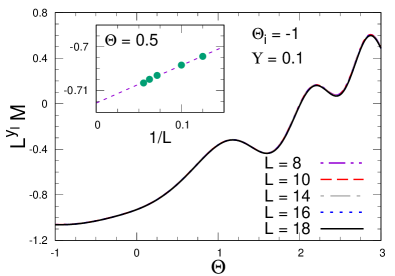
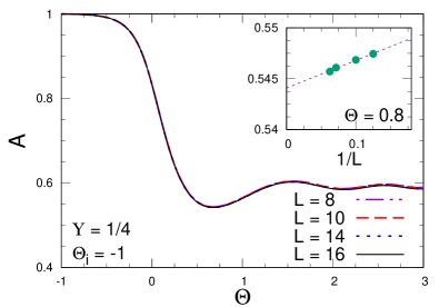
Figure 1: Dynamic FSS of the quantum Ising chain along the one-way KZ protocol at fixed $\Theta_{i}\equiv w_{i}L^{y_{w}}$. We show results for the adiabaticity function $A(t,t_{s},w_{i},L)$ at fixed $\Upsilon=t_{s}/L^{\zeta}=1/4$ and $\Theta_{i}=-1$ up to $L=16$ (bottom) and the longitudinal magnetization $M(t,t_{s},w_{i},L)$ at fixed $\Upsilon=0.1$ and $\Theta_{i}=-1$ up to $L=18$ (top), versus $\Theta=t/t_{s}^{\kappa}$. The exponents $y_{w}$, $\zeta$, and $\kappa$ are reported in Eq. (57). The approach to the large-$t_{s}$ asymptotic behavior is globally characterized by $O(1/L)$ corrections (apart from small superimposed wiggles), as shown by the insets (where the line is drawn to guide the eyes).

Figure 2: Dynamic FSS of the quantum Ising chain along the one-way KZ protocol at fixed $w_{i}<0$. We show the adiabaticity function $A(t,t_{s},w_{i},L)$ up to $L=16$ (bottom) and the longitudinal magnetization $M(t,t_{s},w_{i},L)$ up to $L=18$ (top), at fixed $\Upsilon=1/4$ and $w_{i}=-1/8$, versus $\Theta$. As explained in the text, the scaling behavior emerging at fixed $w_{i}<0$ matches that obtained in the $\Theta_{i}\to-\infty$ limit.

The numerical analyses of quantum Ising chains (2) with a time-dependent longitudinal field is based on exact diagonalization. The corresponding Schrödinger equation is solved using a $4^{\rm th}$ order Runge-Kutta method. This approach allows us to compute the out-of-equilibrium dynamics for lattice size $L\lesssim 20$, which, as we shall see, turns out to be sufficient to achieve a robust evidence of the dynamic FSS outlined in the previous sections, and their problematic aspects.

We want to check the dynamic FSS put forward in Sec. V.1. In the case of the quantum 1D Ising model (3), the exponents entering the definitions of the scaling variables (V.1) are

$$y_{w}=15/8\,,\qquad\zeta=23/8\,,\qquad\kappa=8/23\,.$$ (57)

Some results for the one-way protocol are reported in Figs. 1 and 2, for the adiabaticity function, defined in Eq. (14), and the longitudinal magnetization, defined in Eq. (16), at fixed $\Theta_{i}$ (Fig. 1) and fixed $w_{i}$ (Fig. 2), for lattice sizes up to $L=16$ and $L=18$ respectively (this difference is due to the fact that the computation of the adiabaticity function is heavier). Although the system sizes of the available results are only moderately large, we clearly observe a collapse toward asymptotic scaling curves, thus a robust evidence of the dynamic FSS outlined in Sec. V.1. In particular, the dynamic FSS emerging from the data at fixed $w_{i}<0$ turns out to be independent of the actual fixed value $w_{i}<0$, as predicted by the scaling arguments reported in Sec. V.1 (in Fig. 2 we only show results for $w_{i}=-1/8$, but we have explicitly checked the independence of $w_{i}<0$ of the scaling curves). We note that, as expected, the adiabaticity function significantly drops crossing the quantum transition at finite values of $\Upsilon$, while it remains close to one, i.e. the value corresponding to adiabatic evolutions, for large values of $\Upsilon$. We also note that the data show that the convergence to the asymptotic dynamic FSS is globally consistent with $O(1/L)$ corrections (apart from superimposed wiggles), see the insets of Fig. 1. Analogous corrections are observed for other values of the parameters, in particular when keeping the starting point $w_{i}$ fixed as in Fig. 2.

We remark that the boundary conditions are not particularly relevant for the dynamic scaling behavior of quantum Ising systems when the KZ protocol is driven by the longitudinal field. Analogous scaling behaviors are expected for systems with boundaries, such as open boundary conditions. Note however that, while the power laws are not changed, the dynamic FSS functions depend on the boundary conditions, moreover the presence of boundaries gives rise to further $O(1/L)$ scaling corrections CPV-14 .

Analogous results are obtained for the quantum Kitaev wire, with driving chemical potential. We recall that in this case the choice of the boundary conditions, such as ABC, is essential to guarantee that the KZ protocol connects two gapped phases RV-21 . The corresponding exponents, cf. Eq. (28), entering the definitions of the scaling variables (V.1), are

$$y_{w}=1,\qquad\zeta=2\,,\qquad\kappa=1/2\,.$$ (58)

The simpler integrable nature of the quantum Kitaev wire (4) allows us to easily consider much larger systems, up to $L\approx 10^{3}$, using standard procedures after Fourier transforming to the momentum space. Again the resulting data (not shown) for the adiabaticity function, energy surplus, particle density, and the two-point functions, nicely support the dynamic FSS outlined in Sec. V.1, see also Ref. RV-21 .

We finally mention that other results for one-way KZ protocols within quantum 1D Ising systems can be found in the literature, see e.g. Refs. Dziarmaga-10 ; Dutta-etal-book ; RV-21 and references therein.

VII.2 Along the classical round-trip KZ protocol

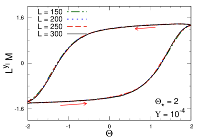
Figure 3: Dynamic FSS behavior of $M(t,t_{s},w_{\star},L)$ for the classical 2D Ising model along the round-trip KZ protocol. Data are obtained at fixed $\Upsilon=10^{-4}$, fixed $\Theta_{\star}=1.5$ (top) and $\Theta_{\star}=2$ (bottom), and are plotted versus $\Theta=w(t)t_{s}^{1-\kappa}$. The arrows indicate the direction of the protocol along the outward and return trip. The values of the exponents $y_{w}$, $\zeta$, and $\kappa$ are reported in Eq. (59). Statistical errors are typically smaller than the thickness of the lines. The convergence to the asymptotic scaling behavior is globally consistent with an $1/L$ approach, see for example the inset of the top figure. Notice that the return trip goes from right to left, because increasing time corresponds to decreasing $\Theta$. We note that the magnetization at the end of the protocol differs from that at the beginning, i.e. for $\Theta=-\Theta_{\star}$ along the outward and backward trip, see Eq. (60). Of course, the values at $\Theta=\Theta_{\star}$ coincide for the two trajectories.

Figure 4: Dynamic FSS behavior of $M(t,t_{s},w_{\star},L)$ for the classical 2D Ising model along the round-trip KZ protocol for fixed $\Upsilon=10^{-4}$, and fixed $w_{\star}=0.02$ and $w_{\star}=0.04$. Statistical errors are typically smaller than the thickness of the lines. The arrows indicate the direction of the protocol along the outward and return trip. These results clearly support the predicted scaling behaviors, see Sec. VI.2, and their independence of the finite value of $w_{\star}>0$.

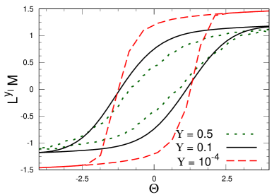
Figure 5: Histeresis curves of the magnetization $M(t,t_{s},w_{\star},L)$ for the classical 2D Ising model along the round-trip KZ protocol for various values of fixed $\Upsilon$. They confirm that the hysteresis area decreases as $\Upsilon$ increases. The curve for $\Upsilon=10^{-4}$ is taken from the data shown in Fig. 4, those for $\Upsilon=0.1$ and $\Upsilon=0.5$ are obtained from simulations for $L=50$, whose size is already sufficient to provide a good approximation of the asymptotic large-$L$ scaling curves (note that Monte Carlo simulations becomes more demanding with increasing $\Upsilon$).

The numerical analysis of the classical Ising model is based on standard Monte Carlo simulations based on local Metropolis upgrading procedures Metropolis:1953am , which provide a purely relaxational dynamics without conserved quantities, that is model A according to the standard classification reported in Ref. HH-77 . The time unit of this dynamics is represented by a global sweep of upgradings of all $L\times L$ spin variables. We perform the single-site update sequentially, moving from one site to one of its neighbours in a typewriter fashion. The results along the time-dependent protocols are obtained by averaging over a sample of trajectories (tipically of order $10^{3}$), starting from an ensemble of thermalized configurations at the initial parameter values. Also in this case relatively large systems can be simulated, typically for $L\gtrsim 10^{2}$.

The dynamic scaling arising from the one-way protocol is quite analogous to that observed at quantum transitions, with corresponding scaling behaviors, characterized by the static Ising critical exponents supplemented by the purely relaxational dynamic exponent $z=2.167(1)$. The corresponding relevant exponents, cf. Eq. (28), entering the definitions of the scaling variables (V.1), are

$$y_{w}=15/8\,,\quad\zeta=4.0420(1)\,,\quad\kappa=0.5361(1)\,.$$ (59)

In the following we only report results for the symmetric round-trip KZ protocols, taking also into account that its first part is equivalent to the one-way KZ protocol.

The dynamic scaling behavior of the magnetization, cf. Eq. (49), is fully supported by the data reported in Fig. 3, for a fixed $\Upsilon=10^{-4}$ and two different values of $\Theta_{\star}$. Analogous results are obtained for other values of $\Upsilon$. As expected the round-trip cycle does not close the curves for finite values of $\Upsilon$ and $\Theta_{\star}$, see Eq. (50), leaving a finite gap between the initial and final values of the cycle, i.e.

$${\cal M}^{(b)}(\Upsilon,-\Theta_{\star},\Theta_{\star})-{\cal M}^{(a)}(\Upsilon,-\Theta_{\star},\Theta_{\star})>0\,,$$ (60)

which becomes smaller and smaller with increasing $\Theta_{\star}$.

As argued in Sec. VI.2, the outward and return trajectories close in the large-$\Theta_{\star}$ limit, and therefore for finite $w_{\star}>0$, giving rise to a critical hysteresis phenomenon. This is clearly demonstrated by the results shown in Fig. 4 for two different finite values of $w_{\star}>0$, whose scaling curves coincide. The outward and return curves for large $|\Theta|$ tend to coincide, differing only within an interval around $\Theta=0$, which becomes smaller and smaller with increasing $\Upsilon$, and vanishes in the adiabatic limit $\Upsilon\to\infty$. Such a dependence on $\Upsilon$ is demonstrated by the curves reported in Fig. 5, showing the magnetization hysteresis for various values of $\Upsilon$. They confirm the scaling law (56) of the hysteresis area. Moreover, we mention that the data at small values of $\Upsilon$ (not shown) hint at a convergence of the scaling hysteresis area ${\cal I}_{A}(\Upsilon)$ to a constant for $\Upsilon\to 0$.

As we shall see, these peculiar behaviors of round-trip protocols developing scaling hysteresis do not have a quantum counterpart, being strictly connected with the fact that the classical purely relaxational dynamics leads eventually to thermalization in the large-time limit when keeping the model parameters fixed.

We also stress that the above hysteresis scenario arises from the round-trip protocols between phases with short-ranged correlations. More complicated situations are expected to occur when round-trip protocols involve ordered phases, where coarsening phenomena may drastically change the picture, in particular along the return trip, in the large-$\Theta_{\star}$ limit.

We finally remark that the boundary conditions do not play a relevant role, indeed analogous scenarios are expected to emerge in classical Ising systems with boundaries, such as open boundary conditions.

VII.3 Along the quantum round-trip KZ protocol

VII.3.1 Scaling for finite $\Theta_{\star}$

Figure 6: Round-trip dynamic FSS of the quantum Ising chain, cf. Eq. (3, for a finite $\Theta_{\star}$. We show results for the adiabaticity function $A(t,t_{s},w_{\star},L)$ at fixed $\Upsilon=t_{s}/L^{\zeta}=0.1$ and $\Theta_{\star}=w_{\star}L^{1-\kappa}=\sqrt{18}$, for the outward (top) and return (bottom) branches of the round-trip KZ protocol, versus $\Theta=w(t)L^{1-\kappa}$, for various size $L$ up to $L=16$. The values of the exponents $y_{w}$, $\zeta$, and $\kappa$ are reported in Eq. (57). Notice that the return trip goes from right to left, because increasing time corresponds to decreasing $\Theta$. The collapse of the curves along both outward and return trips clearly support the dynamic scaling behavior given in Eq. (51).

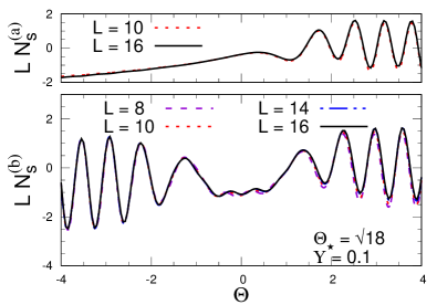
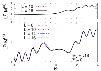
Figure 7: Round-trip dynamic FSS of the longitudinal magnetization $M(t,t_{s},w_{\star},L)$ (bottom figures) and subtracted transverse magnetization $N_{s}(t,t_{s},w_{\star},L)$ (top figures), cf. Eq. (19), in the quantum Ising chain at fixed $\Upsilon=0.1$ and $\Theta_{\star}=\sqrt{18}$, for the outward (top) and return (bottom) branches of the round-trip KZ protocol, versus $\Theta$, for various size $L$ up to $L=16$. The results clearly support the dynamic scaling behavior given in Eq. (49).

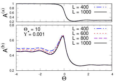
Figure 8: Round-trip dynamic FSS within the quantum Kitaev wire for a finite $\Theta_{\star}=10$. We show results for the adiabaticity function $A(t,t_{s},w_{\star},L)$ at fixed $\Upsilon=t_{s}/L^{\zeta}=0.001$ and $\Theta_{\star}=w_{\star}L^{1-\kappa}=10$, for the outward (top) and return (bottom) branches of the round-trip KZ protocol, versus $\Theta=w(t)L^{1-\kappa}$, for various size $L$ up to $L=1000$. The values of the exponents $y_{w}$, $\zeta$, and $\kappa$ are reported in Eq. (58). The numerical results clearly support the dynamic scaling behavior given in Eq. (51).

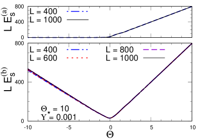
Figure 9: Round-trip dynamic FSS within the quantum Kitaev wire for a finite $\Theta_{\star}=10$. We show results for the surplus energy $E_{s}(t,t_{s},w_{\star},L)$ defined in Eq. (15), at $\Upsilon=t_{s}/L^{\zeta}=0.001$, and $\Theta_{\star}=w_{\star}L^{1-\kappa}=10$, for the outward (top) and return (bottom) branches of the round-trip KZ protocol, versus $\Theta=w(t)L^{1-\kappa}$, for various size $L$ up to $L=1000$. The results clearly support the dynamic scaling behavior given in Eq. (52).

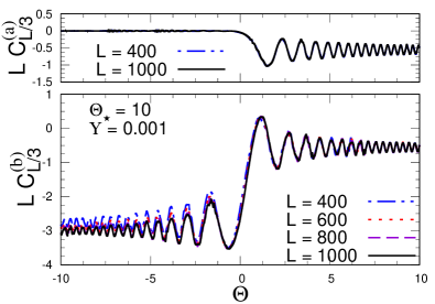
Figure 10: Round-trip dynamic FSS within the quantum Kitaev wire for a finite $\Theta_{\star}$. We show results for the two-point function $C(x,t,t_{s},w_{\star},L)$, cf. Eq. (22), at fixed $X=x/L=1/3$, $\Upsilon=t_{s}/L^{\zeta}=0.001$, and $\Theta_{\star}=w_{\star}L^{1-\kappa}=10$, for the outward (top) and return (bottom) branches of the round-trip KZ protocol, versus $\Theta=w(t)L^{1-\kappa}$, for various size $L$ up to $L=1000$.

To begin with, we show results for round-trip KZ protocols for the quantum Ising chain, cf. Eq. (3), when keeping $\Theta_{\star}$ finite, see Figs. 6 and 7, respectively for the adiabaticity function and the longitudinal and transverse magnetizations. Analogous results are obtained for other values of $\Upsilon$ and $\Theta_{\star}$. Analogous results are also obtained for the quantum Kitaev wire, cf. Eq. (5), see for example the results shown in Figs. 8, 9, and 10, respectively for the adiabaticity function, the surplus energy $E_{s}$ defined in Eq. (15), and the two point function defined in Eq. (22). These results fully support the dynamic FSS put forward in Sec. VI.1 when keeping $\Theta_{\star}$ finite.

VII.3.2 The limit $\Theta_{\star}\to\infty$

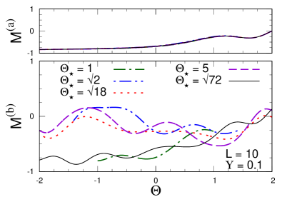
Figure 11: Behavior of $M(t,t_{s},w_{\star},L)$ for fixed $L=10$, $\Upsilon=0.1$ for the one way trip (top) and for the return trip (bottom), versus $\Theta$, for various $\Theta_{\star}$ up to $\Theta_{\star}=6\sqrt{2}$. We note that along the outward path the large-$\Theta_{\star}$ convergence of the curves is rapid (it is essentially related to the convergence with respect to $\Theta_{i}=-\Theta_{\star}$ of the one-way protocol); on the other hand the curves do not appear to approach a large-$\Theta_{\star}$ limit along the return path.

We now discuss the large-$\Theta_{\star}$ limit, and also the related case in which we keep $w_{\star}>0$ fixed in the round-trip protocols. This limit turns out to be quite problematic in quantum round-trip KZ protocols.

Some hints at the absence of a well defined large-$\Theta_{\star}$ limit of the dynamic scaling behavior are shown by the plots of Fig. 11 reporting the longitudinal magnetization of a quantum Ising system of size $L=10$ for various $\Theta_{\star}$. When increasing $\Theta_{\star}$, the curves along the outward way show a good convergence, while no apparent convergence is observed along the return paths.

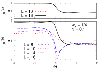
Figure 12: The adiabaticity function $A(t,t_{s},w_{\star},L)$ of quantum Ising chains along round-trip protocols, for fixed $\Upsilon=0.1$ and $w_{\star}=1/4$, for the outward (top) and return (bottom) branches of the round-trip protocol, versus $\Theta$, for various size $L$ up to $L=16$. We note that along the outward path the large-$t_{s}$ convergence is rapid, unlike the return way where no evidence of convergence is observed.

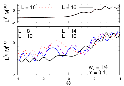
Figure 13: The longitudinal magnetization $M(t,t_{s},w_{\star},L)$ along the round-trip protocol, for fixed $w_{\star}=1/4$, $\Upsilon=0.1$ for the outward (top) and return (bottom) branches of the round-trip protocol, versus $\Theta$, for various size $L$ up to $L=16$.

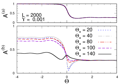
Figure 14: The adiabaticity function $A(t,t_{s},w_{\star},L)$ for the quantum Kitaev wire at $L=2000$ and $\Upsilon=0.001$ for the outward (top) and return (bottom) branches of the round-trip KZ protocol, versus $\Theta$, for various $\Theta_{\star}$ up to $\Theta_{\star}=140$. We note that along the outward path the convergence is large-$\Theta_{\star}$ convergence is rapid (it is essentially related to the convergence with respect to $\Theta_{i}=-\Theta_{\star}$ in the one-way KZ protocol), along the return path the curves do not appear to approach a large-$\Theta_{\star}$ limit.

When we keep $w_{\star}$ fixed and finite, our computations do not show evidence of convergence along the return trajectories in the large-$t_{s}$ and large-$L$ dynamic scaling limit. This is shown by the curves of the adiabaticity function along the return branch of the round-trip protocol, see Fig.12, for $w_{\star}=1/4$ and $\Upsilon=0.1$. While convergence is clearly observed along the outward path, as expected because the one-way KZ protocol showed a well defined limit in the large-$|\Theta_{i}|$ limit, the return path does not show a stable convergence pattern. The same behavior is also shown by the longitudinal and transverse magnetizations $M$ and $N$, see for example Fig. 13. Analogous results are also obtained for the quantum Kitaev wire, see Fig. 14, where we report results for the adiabaticity function at $\Upsilon=0.001$ and various large values of $\Theta_{\star}$, for a large lattice size $L=2000$.

To interpret, and understand, the above instability emerging in quantum systems subject round-trip KZ protocols, it is useful to make a comparison with the dynamic behavior of two-level models subject to analogous round-trip protocols, discussed in App. A. Analogously to the Landau-Zener-Stückelberg problem LZeff ; SAN-10 , we consider a time-dependent two-level Hamiltonian

$$H_{2\ell}(t)=-\beta(t)\sigma^{(3)}+{\Delta\over 2}\sigma^{(1)}\,,$$ (61)

where $\Delta$ is a constant,

$$\beta(t)={{\cal T}(t)\over t_{s}}\quad{\rm for}\;\;t_{i}=-t_{\star}\leq t\leq 3t_{\star}\,,$$ (62)

and ${\cal T}(t)=t_{\star}-|t-t_{\star}|$ is the triangular function. The quantities $\tau={\cal T}(t)/\sqrt{t_{s}}$ and $\tau_{\star}=t_{\star}/\sqrt{t_{s}}$ play the same role of the scaling variables $\Theta$ and $\Theta_{\star}$ describing the round-trip KZ protocols in quantum many-body systems. The corresponding Schrödinger equation can be analytically solved in terms of parabolic cylinder functions $D_{\nu}(x)$ VG-96 , see App. A.

The resulting behavior of the expectation values of $\sigma^{(3)}$ and the adiabatic function show that the large-$\tau_{\star}$ limit is problematic, being characterized by large $O(1)$ oscillations with frequencies increasing proportionally to $\tau_{\star}$, roughly. See App. A for details. They turn out to be related to the rapid changes of the relative phase between the relevant states of the two-level system at the extreme values $\tau=\tau_{\star}$ when $\tau_{\star}$ becomes large, increasing as $\tau_{\star}^{2}$. Since the quantum evolution along the return trajectory turns out to be very dependent on such phase, it becomes extremely sensitive to the value of $\tau_{\star}$, showing analogous oscillations. As a consequence, the value of all observables along the return trajectory, from $\tau=\tau_{\star}$ down to the return point $\tau=-\tau_{\star}$, do not show a well defined limit for $\tau_{\star}\to\infty$. The size of the oscillations depend on the value of the scaling variable $\upsilon=t_{s}\Delta^{2}$, which plays the same role of $\Upsilon$ in the quantum many-body systems, and tend to be suppressed in the adiabatic limit $\upsilon\to\infty$.

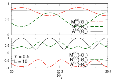
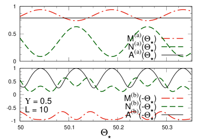
Figure 15: Results for $M,\,N$ and $A$ for fixed $L=10$, $\Upsilon=0.5$ versus $\Theta_{\star}$, close to $\Theta_{\star}=20$ (top figure) and $\Theta_{\star}=50$ (bottom figure). In each figure, the top plot the values of $M^{(a)}$, $N^{(a)}$ and $A^{(a)}$ at the end of the outward branch, corresponding to $\Theta=\Theta_{\star}$, while the bottom plot shows the values of $M^{(b)}$, $N^{(b)}$ and $A^{(b)}$ at the end of the return branch, corresponding to $\Theta=-\Theta_{\star}$. The comparison of the top and bottom figures show that the oscillations tend to become more frequent with increasing $\Theta_{\star}$ (note that the interval of the abscissa is different). Analogous results are obtained for other values of $\Upsilon$.

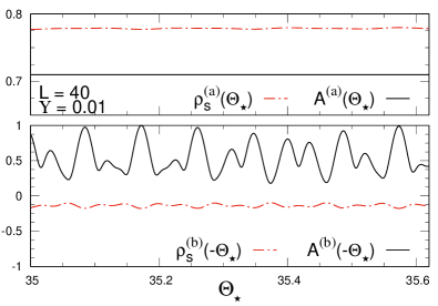
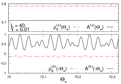
Figure 16: Behavior of the subtracted particle density $\rho_{s}$, cf. Eq. (21), and the adiabaticity function $A$ for the Kitaev wire, for fixed $L=40$, $\Upsilon=0.01$ versus $\Theta_{\star}$, close to $\Theta_{\star}=70$ (bottom figure) and $\Theta_{\star}=35$ (top figure). In each figure, the top plot the values of $\rho_{s}^{(a)}$ and $A^{(a)}$ at the end of the outward branch, corresponding to $\Theta=\Theta_{\star}$, while the bottom plot shows the values of $\rho_{s}^{(b)}$ and $A^{(b)}$ at the end of the return branch, corresponding to $\Theta=-\Theta_{\star}$. Again, the comparison of the top and bottom figures show that the oscillations tend to become more frequent with increasing $\Theta_{\star}$.

We observe a similar behavior in the quantum many-body systems. This scenario is demonstrated by the results shown in Fig. 15, where we report the values of $A^{(a)}$, $M^{(a)}$, and $N^{(a)}$ at end of the outward branch and $A^{(b)}$, $M^{(b)}$, and $N^{(b)}$ at the end of the return branch, for KZ protocols with different $\Theta_{\star}$, to check their large-$\Theta_{\star}$ convergence, for some interval of values of $\Theta_{\star}$ around large values of $\Theta_{\star}$ and fixed $L=10$. Similarly to the results obtained for two-level model, the observables at the end of the outward branch oscillate, with a frequency that becomes larger and larger with increasing $\Theta_{\star}$, and the oscillations observed after the whole cycle are strongly correlated to those at the end of the first branch, doubling the frequency. Analogous results are obtained for other values of $\Upsilon$. We also note that the oscillations tend to be suppressed in the adiabatic $\Upsilon\to\infty$ limit. We believe that this extreme sensitivity to $\Theta_{\star}$ makes also problematic the large-$L$ limit after the limit $\Theta_{\star}\to\infty$ shown by the numerical data. Similar results are also obtained for the quantum Kitaev wire, see Fig. 16 where we show results for the adiabaticity function and the particle density. In this case the values at the end of the outward way appear quite stable, but the return way is again characterized by large (less regular) oscillations with larger and larger frequencies with increasing $\Theta_{\star}$.

The above results for both the quantum Ising rings and Kitaev wires strongly suggest that in quantum many-body systems the large-$\Theta_{\star}$ limit of the dynamic KZ scaling does not exist along the return trajectories, and, as a consequence, no dynamic scaling is observed along the return trip when $w_{f}>0$ is kept fixed and finite in the round-trip KZ protocols. In this respect, there are notable similarities with the behavior of two-level model (61) subject to round-trip protocols. We believe that this issue deserves further investigation, for example addressing the possibility of obtaining well defined scaling behavior after some average procedures over the oscillations induced by large values of $\Theta_{\star}$, to obtain a well defined large-$\Theta_{\star}$ limit.

However, we stress that the dynamic scaling behavior is nicely observed when keeping $\Theta_{\star}$ fixed, even along the return trajectory. This may be related to fact that, when keeping $\Theta_{\star}$ fixed, the time scaling variable $\Theta$ remains finite, therefore the time variable is always rescaled consistently with the time scale of the equilibrium quantum transition, provided by the inverse gap at the transition, i.e. $\Delta\sim L^{-z}$ at the critical point, or $\Delta\sim\lambda^{-z}$ in the thermodynamic limit, where $\lambda$ is the KZ length scale (45). As a consequence, the interval of values of $w(t)$ remains limited within a small interval around the transition, which becomes smaller and smaller in the large-size limit, as $|w|\lesssim L^{-y_{w}}$, and the relative quantum phases behave consistently with the scaling laws.

VIII Conclusions

We have studied the out-of-equilibrium behavior of many-body systems when their time-dependent Hamiltonian parameters slowly cross phase transition points, where systems at equilibrium develop critical modes with long-range correlations. Earlier studies have already shown the emergence of several interesting out-of-equilibrium phenomena, such as hysteresis, coarsening, KZ defect production, aging, etc.. In this paper we present an exploratory study of out-of-equilibrium behaviors arising from round-trip protocols across classical and quantum phase transitions.

We consider classical and quantum many-body systems described by the general Hamiltonian (1), and study the out-of-equilibrium evolution arising from cyclic variations of the parameter $w$ driving the equilibrium transition, entailing multiple crossings of the transition point $w_{c}=0$. More precisely, we consider round-trip protocols where the many-body system starts from equilibrium conditions at a given value $w_{i}<0$, and the out-of-equilibrium dynamics is driven by changing the parameter $w(t)$ in Eq. (1) linearly in time up to $w_{f}>0$, thus crossing the critical point $w_{c}=0$, and then by changing it back to the original value $w_{i}<0$, again linearly in time, which implies a further crossing of the transition point. The round-trip protocol is characterized by a unique large time scale $t_{s}$, see Sec. III.2. We limit our study to the cases where the transition point separates phases with short-range correlations. The more complicated situations of classical and quantum transitions between disordered and ordered phases with ungapped excitations is left to future works.

We address these issues within many-body models undergoing classical and quantum transitions, exploiting a unified RG framework, where general dynamic scaling laws are derived in the large-$t_{s}$ and large-$L$ limits, see Secs. V and VI. In particular, we extend the RG framework already developed for standard one-way KZ protocols, see e.g. Refs. CEGS-12 ; RV-21 .

As paradigmatic models, we consider classical and quantum systems that undergo classical and quantum transitions belonging to the 2D Ising universality class: (i) Classical 2D Ising models undergoing a finite-temperature transition, supplemented with a purely relaxational dynamics driven by an external time-dependent magnetic field; (ii) Quantum 1D Ising models with an external time-dependent longitudinal field; (iii) Quantum 1D Kitaev fermionic wires with a time-dependent chemical potential. In all cases we analyze the out-of-equilibrium behavior arising from round-trip linear variations of the Hamiltonian parameters, crossing twice the transition point. We report various numerical analyses of one-way and round-trip KZ protocols within the above models, see Sec. VII. They generally support the dynamic FSS behaviors in the large time-scale ($t_{s}$) limit, put forward within the RG frameworks.

However, while the general dynamic scaling picture may appear similar, there are also important differences between classical and quantum systems. Indeed, the analogy of the scaling behaviors for one-way KZ protocols at classical and quantum transitions is only partially extended to round-trip KZ protocols. Substantial differences emerge, in particular when the extreme value $w_{f}>0$ of the outward variation of $w(t)$ is kept fixed and finite in the large-$t_{s}$ limit. On the one hand, classical systems show a well-defined dynamic scaling limit, developing scaling hysteresis-like scenarios, essentially because the purely relaxational stochastic dynamics leads eventually to thermalization at fixed model parameters. On the other hand, in quantum systems the observation of scaling behavior along the return way turns out to be more problematic, due to the persistence of rapidly oscillating relative phases between the relevant quantum states. They make the return way extremely sensitive to the parameters of the protocol, such as the extreme value $w_{f}$ and the size $L$ of the system. This is essentially related to the quantum nature of the dynamics. Indeed there are some notable similarities with the behavior of quantum two-level models subject to round-trip protocols, analogous the well-known Landau-Zener-Stückelberg problem LZeff ; SAN-10 ; ISN-22 , see App. A. Even in the simple two-level quantum model some features of the behavior along the return way turn out not to be smooth. Indeed, they develop ample oscillations with larger and larger frequencies when increasing the interval of the round-trip variation of the parameters, showing chaotic-like behaviors due to the extreme sensitivity to the protocol parameters. We believe that this issue calls for further investigation, to achieve a better understanding of these phenomena.

The emerging dynamic scaling scenario put forward for round-trip KZ protocols across critical points is expected to hold for generic classical and quantum transitions separating phases with short-range correlations, in any spatial dimension. Further investigations are called for round-trip protocols between disordered and ordered phases, when the ordered phase has gapless excitations. Round-trip KZ protocols in these systems may show further interesting features.

In this paper we have focused on continuous transitions. Analogous issues may be investigated at first-order classical and quantum transitions, where dynamic scaling behaviors emerge as well, although they turn out to significantly depend on the nature of the boundary conditions (see e.g. Refs Binder-87 ; RV-21 ; PRV-18 ; CNPV-14 ; PV-17 ; PV-17-a ; PRV-20 ; DOV-09 for studies at classical and quantum transitions). Further interesting issues may concern the effects of dissipation due to the interaction with an environment, which are inevitable in realistic quantum devises, and can induce some further relevant effects in the dynamics of systems subject to round-trip KZ protocols, see e.g. Refs. RV-21 ; FFO-07 ; PSAFS-08 ; PASFS-09 ; YMZ-14 ; NVC-15 ; KMSFR-17 ; SVPKD-17 ; ABRS-18 ; NRV-19-dis ; RV-19-dis ; RV-20 .

We remark that round-trip protocols at classical and quantum transitions should also be of experimental relevance. Indeed they represent a straightforward extension of the one-way KZ protocols, which have been already investigated experimentally at both thermal and quantum transitions, as already mentioned in the introduction.

Our results may turn out to be particularly relevant for quantum simulations and quantum computing, where important experimental advances have been achieved recently, see e.g. Refs. CZ-12 ; BDN-12 ; BR-12 ; AW-12 ; HTK-12 ; GAN-14 . In particular, our results imply some limitations to the observation of a round-trip dynamics across quantum transitions in many-body models. We also note that the dynamic scaling behavior put forward in this work have been observed in numerical simulations of systems of moderately large size. This suggests the possibility that the dynamic scaling scenario may be accessed by experiments with quantum simulators in laboratories, e.g., by means of trapped ions Islam-etal-11 ; Debnath-etal-16 , ultracold atoms Simon-etal-11 ; Labuhn-etal-16 , or superconducting qubits Salathe-etal-15 ; Cervera-18 .

Appendix A Round-trip Landau-Zener protocols in two-level models

In this section we study time-dependent round-trip protocols within a paradigmatic two-level model, described by the Hamiltonian (61). Their quantum evolution is ruled by the Schrödinger equation

$$i\,\partial_{t}\Psi(t)=H_{2\ell}(t)\Psi(t)\,,$$ (63)

$$H_{2\ell}(t)=-\beta(t)\sigma^{(3)}+{\Delta\over 2}\sigma^{(1)}\,.$$

The parameter $\Delta$ corresponds to the energy difference of the Hamiltonian eigenstates at $\beta(t)=0$. To describe the states $\Psi(t)$ of the system, we consider the diabatic basis provided by the eigenvectors $|+\rangle$ and $|-\rangle$ of $\sigma^{(3)}$, with eigenvalues $1$ and $-1$, respectively. Therefore, we may write

$$\Psi(t)=\phi_{1}(t)|+\rangle+\phi_{2}(t)|-\rangle\,,$$ (64)

and define $\Psi(t)\equiv[\phi_{1}(t),\phi_{2}(t)]$. It is convenient to define

$$\eta(t)={2\beta(t)\over\Delta}\,,$$ (65)

so that

$$H_{2\ell}(t)={\Delta\over 2}\,\widetilde{H}_{2\ell}(t)\,,\quad\widetilde{H}_{2\ell}(t)=-\eta(t)\sigma^{(3)}+\sigma^{(1)}\,.$$ (66)

Adiabatic time evolutions, i.e. for sufficiently slow changes of the Hamiltonian parameter $\eta(t)$, pass through the stationary eigenstates of $H_{2\ell}$ at fixed $\eta(t)=\eta$, which are given by

$$|\Psi_{0},\eta\rangle={\cal N}_{0}(\eta)\left[(-\eta-\sqrt{1+\eta^{2}})|+\rangle+|-\rangle\right]\,,$$

$$E_{0}=-{\Delta\over 2}\sqrt{1+\eta^{2}}\,,$$ (67)

$$|\Psi_{1},\eta\rangle={\cal N}_{1}(\eta)\left[(-\eta+\sqrt{1+\eta^{2}})|+\rangle+|-\rangle\right]\,,$$

$$E_{1}={\Delta\over 2}\sqrt{1+\eta^{2}}\,,$$ (68)

where ${\cal N}_{i}(\eta)$ are appropriate normalizations so that $\langle 0|0\rangle=\langle 1|1\rangle=1$.

In the following we consider a linear time dependence of the Hamiltonian parameter $\beta(t)$, and round-trip linear protocols. We start at $t_{i}=-t_{\star}$ from the ground state $|\Psi_{0},\eta_{i}\rangle\equiv[\phi_{1}^{(0)},\phi_{2}^{(0)}]$ of the system for $\beta(t_{i})$. Then the system evolves according to the Schrödinger equation (63) with $\beta(t)$ given by the Eq. (62), i.e. $\beta(t)={{\cal T}(t)/t_{s}}$ for $t_{i}=-t_{\star}\leq t\leq 3t_{\star}$, where ${\cal T}(t)=t_{\star}-|t-t_{\star}|$ is the triangular function going linearly from ${\cal T}(-t_{\star})=-t_{\star}$ to ${\cal T}(t_{\star})=t_{\star}$, and then back to ${\cal T}(3t_{\star})=-t_{\star}$. The parameter $t_{s}$ represents the time scale of the variation. The parameter $t_{\star}>0$ controls the extension (i.e. the starting and final times) of the protocols, from $t_{i}=-t_{\star}$ to $t_{f}=3t_{\star}$, and also the interval of variation of $\beta(t)$, from $\beta(t_{i})=-t_{\star}/t_{s}$ to $\beta(t_{\star})=t_{\star}/t_{s}$. An analogous cyclic time dependence is considered in the so-called Landau-Zener-Stückelberg problem, see e.g. Refs. SAN-10 ; ISN-22 and references therein.

To solve this problem, it is convenient to introduce the variables

$$\tau={{\cal T}(t)\over\sqrt{t_{s}}}\,,\qquad\tau_{\star}={t_{\star}\over\sqrt{t_{s}}}\,,\qquad\upsilon=t_{s}\Delta^{2}\,,\qquad$$ (69)

$$\kappa={2\tau\over\sqrt{\upsilon}}={2\beta(t)\over\Delta}\,,\qquad\kappa_{\star}={2\tau_{\star}\over\sqrt{\upsilon}}\,.$$ (70)

Then the time evolution can be straightforwardly determined using the results of Ref. VG-96 , in terms of parabolic cylinder functions $D_{\nu}(x)$ Abrafunc . Along the first branch from $-t^{\star}$ to $t^{\star}$, we write

$$\phi_{i}^{(1)}(\tau)=U_{ij}(\tau,\tau_{i})\phi_{j}^{(0)}\,,$$ (71)

where $\tau=t/\sqrt{t_{s}}$ with $-t_{\star}\leq t\leq t_{\star}$, $\tau_{i}=-\tau_{\star}$, and the evolution matrix elements are VG-96

$$U_{11}(\tau,\tau_{i})={\Gamma(1-i\upsilon/8)\over\sqrt{2\pi}}\times$$ (72)

$$\quad\Big{[}D_{i\upsilon/8}(\sqrt{2}e^{-i\pi/4}\tau)\,D_{-1+i\upsilon/8}(\sqrt{2}e^{i3\pi/4}\tau_{i})+$$

$$\quad\;\;\;D_{i\upsilon/8}(\sqrt{2}e^{i3\pi/4}\tau)\,D_{-1+i\upsilon/8}(\sqrt{2}e^{-i\pi/4}\tau_{i})\Big{]}\,,$$

$$U_{12}(\tau,\tau_{i})={2\Gamma(1-i\upsilon/8)e^{i\pi/4}\over\sqrt{\pi\upsilon}}\times$$

$$\quad\Big{[}-D_{i\upsilon/8}(\sqrt{2}e^{-i\pi/4}\tau)\,D_{i\upsilon/8}(\sqrt{2}e^{i3\pi/4}\tau_{i})+$$

$$\quad\;\;\;D_{i\upsilon/8}(\sqrt{2}e^{i3\pi/4}\tau)\,D_{i\upsilon/8}(\sqrt{2}e^{-i\pi/4}\tau_{i})\Big{]}\,,$$

$$U_{21}=-U_{12}^{*}\,,\qquad U_{22}=U_{11}^{*}\,.$$

Using the properties of the evolution matrix $U$ under the transformation $\eta(t)\to-\eta(t)$ VG-96 , we can write the evolution for $t>t^{\star}$ as

$$\phi_{i}^{(2)}(\tau)=V_{ij}(\tau_{b},\tau_{i})\phi_{j}^{(1)}(\tau_{\star})\,,$$ (73)

where $\tau$ is defined as in Eq. (69), thus it is decreasing from $\tau_{\star}$ to $-\tau_{\star}$, again $\tau_{i}=-t_{\star}/\sqrt{t_{s}}$, $\tau_{b}=t_{b}/\sqrt{t_{s}}$ with $t_{b}=t-2t_{\star}$, and the functions $V_{ij}$ are closely related to $U_{ij}$: VG-96

$$V_{11}=U_{11}^{*}\,,\qquad V_{12}=-U_{12}^{*}\,,$$

$$V_{22}=U_{22}^{*}\,,\qquad V_{21}=-U_{21}^{*}\,.\quad$$

Note that these expressions are consistent with those used for the Landau-Zener-Stückelberg problem in the presence of Hamiltonian parameters with cyclic time dependence as in Eq. (63), see e.g. Refs. SAN-10 ; ISN-22 .

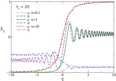
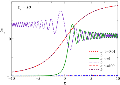
Figure 17: Evolution of $S_{3}$ during the round-trip protocol, for $\tau_{\star}=10$ (bottom) and $\tau_{\star}=20$ (top), and some values of $\upsilon$.

Since the scaling variable $\tau$ related to time takes the same values in the intervals $-t_{\star}\leq t\leq t_{\star}$ and $t_{\star}\leq t\leq 3t_{\star}$, we separate the time dependence in two parts: ($a$) for the first part where $\beta(t)$ and $\tau$ increases, and ($b$) where $\beta(t)$ and $\tau$ decreases. We monitor the dynamic evolution along the protocol defined above by the expectation values of the operators $\sigma^{(k)}$, i.e.

$$S_{3}^{(a/b)}(\upsilon,\tau,\tau_{\star})=\langle\Psi(t)|\sigma^{(3)}|\Psi(t)\rangle\,,$$ (75)

$$S_{1}^{(a/b)}(\upsilon,\tau,\tau_{\star})=\langle\Psi(t)|\sigma^{(1)}|\Psi(t)\rangle\,,$$ (76)

and the adiabaticity function

$$A^{(a/b)}(\upsilon,\tau,\tau_{\star})=|\langle\,\Psi_{0},\eta(t)\,|\,\Psi(t)\,\rangle|\,.$$ (77)

Again, the superscripts $(a)$ and $(b)$ refer to the outward and return trip, respectively. Note that the adiabatic limit of the evolution is obtained by sending $\upsilon\to\infty$ keeping fixed $\kappa$. Therefore,

$$\lim_{\upsilon\to\infty}A^{(a/b)}(\upsilon,\kappa\sqrt{\upsilon}/2,\kappa_{\star}\sqrt{\upsilon}/2)=1\,.$$ (78)

Some results for the magnetization $S_{3}$ are shown in Fig. 17 along the first and second branch of the protocol, for various values of $\upsilon$, $\upsilon=0.1,\,1,\,10$, and $\tau_{\star}=10,\,20$. As expected, the case of large $\upsilon$ the dynamic tends to be adiabatic, so that the values of $S_{3}$ along the two ways tend to superimpose. In the case of small $\upsilon$ the dyamic tends to be frozen to the initial condition, moving only slightly from the initial value. More complex behaviors are observed for intermediate values of $\upsilon$.

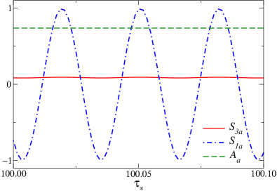
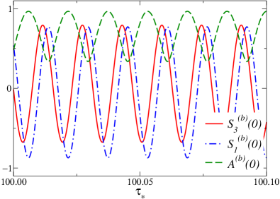
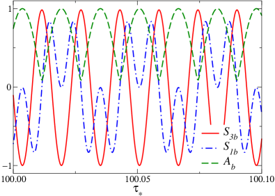
Figure 18: Dependence on $\tau_{\star}\equiv t_{\star}/\sqrt{t_{s}}$ of the magnetizations $S_{1/3}$ and the adiabaticity function $A$ at the end of the first dynamic branch where $\beta(t)$ is linearly increasing, and then back along the return way, when $\tau=0$ (intermediate) and at the end of the round-trip protocol (bottom), for $\upsilon=1$, and $\tau_{\star}\approx 100$. These results show clearly how the oscillations of $S_{1,a}$, and therefore of the relative phase of the two functions $\phi_{i}(t)$ in Eq. (64), at the end of the first branch are closely related to the oscillations of all observables along the return way of the round-trip protocol.

We now analyze the dynamics of the round-trip protocol in the large-$\tau_{\star}$ limit, showing that such limit is problematic for this problem. We consider the values of the above observables at the end of the first and second part of the protocol:

$$S_{3/1a}(\upsilon,\tau_{\star}) = S_{3/1}^{(a)}(\upsilon,\tau_{\star},\tau_{\star})\,,$$ (79)

$$S_{3/1b}(\upsilon,\tau^{\star}) = S_{3/1}^{(b)}(\upsilon,-\tau_{\star},\tau_{\star})\,,$$

$$A_{a}(\upsilon,\tau_{\star}) = A^{(a)}(\upsilon,\tau_{\star},\tau_{\star})\,,$$

$$A_{b}(\upsilon,\tau_{\star}) = A^{(b)}(\upsilon,-\tau_{\star},\tau_{\star})\,.$$

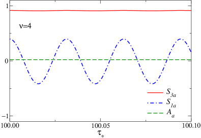
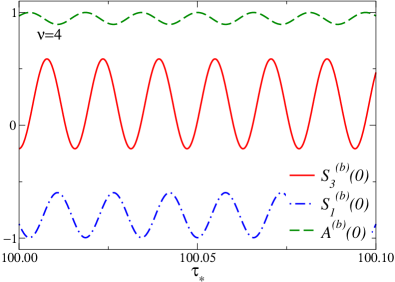
Figure 19: Dependence on $\tau_{\star}\equiv t_{\star}/\sqrt{t_{s}}$ of the magnetizations $S_{1/3}$ and the adiabaticity function $A$ at the end of the first dynamic branch where $\beta(t)$ is linearly increasing, and then along the return way, when $\tau=0$ (bottom), for $\upsilon=4$, and $\tau_{\star}\approx 100$.

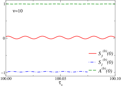
Figure 20: Dependence on $\tau_{\star}\equiv t_{\star}/\sqrt{t_{s}}$ of the magnetizations $S_{1/3}$ and the adiabaticity function $A$ along the return way at $\tau=0$, for $\upsilon=10$, and $\tau_{\star}\approx 100$.

Some notable limits can be derived for the first branch of the protocol using the asymptotic behaviors of the parabolic cylinder functions $D_{\nu}(x)$ VG-96 ; ISN-22 , corresponding to the standard Landau-Zener problem, see e.g. Refs. VG-96 ; PRV-18-loc , such as

$$S_{3a}(\upsilon,\tau_{\star}\to\infty)=1-2\,e^{-{\pi\upsilon/4}}\,,\qquad$$ (80)

$$A_{a}(\upsilon,\tau_{\star}\to\infty)=\sqrt{1-\,e^{-{\pi\upsilon/4}}}\,.$$

Both $S_{3a}$ and $A_{a}$ approach their asymptotic behaviors with oscillating corrections suppressed as $O(\tau_{\star}^{-1})$. For example, in the case of the adiabaticity function we find

$$\Delta A_{a} \equiv A_{a}(\upsilon,\tau_{\star})-A_{a}(\upsilon,\infty)$$

$$\approx {f(\upsilon)\over\tau_{\star}}\cos[\tau_{\star}^{2}-{u\over 4}\ln\tau_{\star}+g(\upsilon)]\,,$$

where $f$ and $g$ are time-independent functions of $\upsilon$ only. Unlike $S_{3a}$ and $A_{a}$, the quantity $S_{1a}$ does not show a regular large-$\tau_{\star}$ limit, but rapid oscillations with diverging frequency in the large-$\tau^{*}$ limit. Indeed, using again the asymptotic behaviors of the parabolic cylinder functions $D_{\nu}(x)$ VG-96 ; ISN-22 , the asymptotic large-$\tau_{\star}$ behavior of $S_{1,a}$ turns out to be

$$S_{1a}\approx B(\upsilon)\cos\varphi(\upsilon,\tau_{\star})\,,\qquad$$ (82)

$$B(\upsilon)=2\,e^{-\pi\upsilon/8}\,\sqrt{1-e^{-\pi\upsilon/4}}\;\leq 1\,,$$

$$\varphi(\upsilon,\tau_{\star})=\tau_{\star}^{2}+{\upsilon\over 8}\ln(2\tau_{\star}^{2})-{\rm Arg}\left[\Gamma\left(i{\upsilon\over 8}\right)\right]+{3\pi\over 4}\,.$$

In particular, $B(1)=0.99611...$ and

$$\varphi(1,\tau_{\star})=\tau_{\star}^{2}+{1\over 4}\ln\tau_{\star}+4.08501...$$ (83)

Unlike $S_{3a}$ and $A_{a}$ that converge to a large-$\tau_{\star}$ limit, the leading behavior of $S_{1a}$ is characterized by rapid oscillations. Its oscillatory behavior is essentially related to the relative phase $e^{-i\varphi(u,\tau)}$ of the functions $\phi_{1}(u,\tau)$ and $\phi_{2}(u,\tau)$, cf. Eq. (64). Note that oscillations become faster and faster in the large-$\tau^{\star}$ limit, with a time-dependent frequency $\omega(\tau_{\star})$ diverging as $\omega(\tau_{\star})\approx\tau_{\star}$. Therefore, unlike $S_{3a}$ and $A_{a}$ whose oscillations gets suppressed as $1/\tau_{\star}$ approximately, the quantity $S_{1a}$ does not possess a well defined large-$\tau_{\star}$ limit, reflecting the fact that the relative phase of the $\phi_{i}$ does not converge in the large-$\tau_{\star}$ limit.

This fact has dramatic implications for the behavior of the system along the backward branch, making all quantities rapidly oscillating at the return point, with a frequency related to that of the relative phase at the end of the first branch. This behavior is clearly shown in Figs. 18, where we report some results for the quantities defined in Eqs. (79), at the end of the outward branch, and along the return branch at $\tau=0$ and at the end of the round-trip protocol, at fixed $\upsilon=1$ and as a function of the parameter $\tau_{\star}$, for a relatively small interval around $\tau_{\star}\approx 100$. As shown by the analogous curves reported in Figs. 19 and 20 for $\nu=4$ and $\nu=10$ respectively, the size of the oscillations depends on the value of $\nu$, and, as expected, it tends to decreases in the adiabatic limit when increasing $\nu$.

These results evidentiate the peculiar oscillations in the large-$\tau_{\star}$ limit at finite values of $\nu$, which make predictions on the return behavior practically impossible without an extreme precision on the control of the parameters of the protocols.

References

- (1) T. W. B. Kibble, Topology of Cosmic Strings and Domains, J. Phys. A 9, 1387 (1976).
- (2) T. W. B. Kibble, Some implications of a cosmological phase transition, Phys. Rep. 67, 183 (1980).
- (3) K. Binder, Theory of first-order phase transitions, Rep. Prog. Phys. 50, 783 (1987).
- (4) I. Chuang, R. Durrer, N. Turok, and B. Yurke, Cosmology in the Laboratory: Defect Dynamics in Liquid Crystals, Science 251, 1336 (1991).
- (5) M. J. Bowick, L. Chandar, E. A. Schiff, and A. M. Srivastava, The Cosmological Kibble Mechanism in the Laboratory: String Formation in Liquid Crystals, Science 263, 943 (1994).
- (6) A. J. Bray, Theory of phase-ordering kinetics, Adv. Phys. 43, 357 (1994).
- (7) W. H. Zurek, Cosmological experiments in condensed matter systems, Phys. Rep. 276, 177 (1996).
- (8) C. Bäuerle, Yu M. Bunkov, S. N. Fisher, H. Godfrin, and G. R. Pickett, Laboratory simulation of cosmic string formation in the early Universe using superfluid 3He, Nature 382, 332 (1996).
- (9) P. Calabrese and A. Gambassi, Ageing properties of critical systems, J. Phys. A: Math. Gen. 38, R133 (2005).
- (10) D. Boyanovsky, H. J. de Vega, and D. J. Schwarz, Phase transitions in the early and the present universe, Annu. Rev. Nucl. Part. Sci. 56, 441 (2006).
- (11) C. N. Weiler, T. W. Neely, D. R. Scherer, A. S. Bradley, M. J. Davis, and B. P. Anderson, Spontaneous vortices in the formation of Bose–Einstein condensates, Nature 455, 948 (2008).
- (12) J. Dziarmaga, Dynamics of a quantum phase transition and relaxation to a steady state, Adv. Phys. 59, 1063 (2010).
- (13) A. Polkovnikov, K. Sengupta, A. Silva, and M. Vengalattore, Colloquium: Nonequilibrium dynamics of closed interacting quantum systems, Rev. Mod. Phys. 83, 863 (2011).
- (14) S. Ulm, S. J. Roßnagel, G. Jacob, C. Degünther, S. T. Dawkins, U. G. Poschinger, R. Nigmatullin, A. Retzker, M. B. Plenio, F. Schmidt-Kaler, and K. Singer, Observation of the Kibble-Zurek scaling law for defect formation in ion crystals, Nat. Commun. 4, 2290 (2013).
- (15) K. Pyka, J. Keller, H. L. Partner, R. Nigmatullin, T. Burgermeister, D. M. Meier, K. Kuhlmann, A. Retzker, M. B. Plenio, W. H. Zurek, A. del Campo, and T. E. Mehlstäubler, Topological defect formation and spontaneous symmetry breaking in ion Coulomb crystals, Nat. Commun. 4, 2291 (2013).
- (16) N. Navon, A. L. Gaunt, R. P. Smith, and Z. Hadzibabic, Critical dynamics of spontaneous symmetry breaking in a homogeneous Bose gas, Science 347, 167, (2015).
- (17) G. Biroli, Slow relaxations and nonequilibrium dynamics in classical and quantum systems, in Strongly interacting quantum systems out of equilibrium: Lecture notes of the Les Houches Summer School, Aug. 2012, (Oxford University Press, 2016).
- (18) A. Trenkwalder, G. Spagnolli, G. Semeghini, S. Coop, M. Landini, P. Castilho, L. Pezzè, G. Modugno, M. Inguscio, A. Smerzi, and M. Fattori, Quantum phase transitions with parity-symmetry breaking and hysteresis, Nat. Phys. 12, 826 (2016).
- (19) D. Rossini and E. Vicari, Coherent and dissipative dynamics at quantum phase transitions, Phys. Rep. 936, 1 (2021).
- (20) A. Polkovnikov, Universal adiabatic dynamics in the vicinity of a quantum critical point, Phys. Rev. B 72, 161201(R) (2005).
- (21) W. H. Zurek, U. Dorner, and P. Zoller, Dynamics of a quantum phase transition, Phys. Rev. Lett. 95, 105701 (2005).
- (22) J. Dziarmaga, Dynamics of a quantum phase transition: Exact solution of the quantum Ising model, Phys. Rev. Lett. 95, 245701 (2005).
- (23) C. De Grandi, V. Gritsev, and A. Polkovnikov, Quench dynamics near a quantum critical point, Phys. Rev. B 81, 012303 (2010).
- (24) S. Gong, F. Zhong, X. Huang, and S. Fan, Finite-time scaling via linear driving, New J. Phys. 12, 043036 (2010).
- (25) A. Chandran, A. Erez, S. S. Gubser, and S. L. Sondhi, Kibble-Zurek problem: Universality and the scaling limit, Phys. Rev. B 86, 064304 (2012).
- (26) A. Pelissetto, D. Rossini, and E. Vicari, Out-of-equilibrium dynamics driven by localized time-dependent perturbations at quantum phase transitions, Phys. Rev. B 97, 094414 (2018).
- (27) A. Pelissetto, D. Rossini, and E. Vicari, Dynamic finite-size scaling after a quench at quantum transitions, Phys. Rev. E 97, 052148 (2018).
- (28) D. Rossini and E. Vicari, Scaling of decoherence and energy flow in interacting quantum spin systems, Phys. Rev. A 99, 052113 (2019).
- (29) W. H. Zurek, Cosmological Experiments in Superfluid Helium?, Nature 317, 505 (1985).
- (30) A. Polkovnikov and V. Gritsev, Breakdown of the adiabatic limit in low-dimensional gapless systems, Nature Phys. 4, 477 (2008).
- (31) A. Dutta, G. Aeppli, B. K. Chakrabarti, U. Divakaran, T. F. Rosenbaum, and D. Sen, Quantum phase transitions in transverse field spin models: From statistical physics to quantum information, Cambridge University Press (2015).
- (32) A. Pelissetto and E. Vicari, Off-equilibrium scaling behaviors driven by time-dependent external fields in three-dimensional O() vector models, Phys. Rev. E 93, 032141 (2016).
- (33) D. Rossini and E. Vicari, Dynamic Kibble-Zurek scaling framework for open dissipative many-body systems crossing quantum transitions, Phys. Rev. Research 2, 023611 (2020).
- (34) B. Damski, The simplest quantum model supporting the Kibble-Zurek mechanism of topological defect production: Landau-Zener transitions from a new perspective, Phys. Rev. Lett. 95, 035701 (2005).
- (35) M. Uhlmann, R. Schützhold, and U. R. Fischer, Vortex quantum creation and winding number scaling in a quenched spinor Bose gas, Phys. Rev. Lett. 99, 120407 (2007).
- (36) M. Uhlmann, R. Schützhold, and U. R. Fischer, System size scaling of topological defect creation in a second-order dynamical quantum phase transition, New. J. Phys. 12, 095020 (2010).
- (37) T. Nag, A. Dutta, and A. Patra, Quench dynamics and quantum information, Int. J. Mod. Phys. B 27, 1345036 (2013).
- (38) A. del Campo and W. H. Zurek, Universality of phase transition dynamics: Topological defects from symmetry breaking, Int. J. Mod. Phys. A 29, 1430018 (2014).
- (39) M. M. Rams, J. Dziarmaga, and W. H. Zurek, Symmetry Breaking Bias and the Dynamics of a Quantum Phase Transition, Phys. Rev. Lett. 123, 130603 (2019).
- (40) J. Rysti, J. T. Maäkinen, S. Autti, T. Kamppinen, G. E. Volovik, and V. B. Eltsov, Suppressing the Kibble-Zurek Mechanism by a Symmetry-Violating Bias, Phys. Rev. Lett. 127, 115702 (2021).
- (41) S. Ducci, P. L. Ramazza, W. Gonzáles-Viñas, and F. T. Arecchi, Order parameter fragmentation after a symmetry-breaking transition, Phys. Rev. Lett. 83, 5210 (1999).
- (42) R. Monaco, J. Mygind, M. Aaroe, R. J. Rivers, and V. P. Koshelets, Zurek-Kibble mechanism for the spontaneous vortex formation in Nb-Al/Alox/Nb Josephson tunnel junctions: New theory and experiment, Phys. Rev. Lett. 96, 180604 (2006).
- (43) L. E. Sadler, J. M. Higbie, S. R. Leslie, M. Vengalattore, and D. M. Stamper-Kurn, Spontaneous symmetry breaking in a quenched ferromagnetic spinor Bose–Einstein condensate, Nature 443, 312 (2006).
- (44) D. Chen, M. White, C. Borries, and B. DeMarco, Quantum quench of an atomic Mott insulator, Phys. Rev. Lett. 106, 235304 (2011).
- (45) S. M. Griffin, M. Lilienblum, K. T. Delaney, Y. Kumagai, M. Fiebig, and N. A. Spaldin, Scaling behavior and beyond equilibrium in the hexagonal manganites, Phys. Rev. X 2, 041022 (2012).
- (46) G. Lamporesi, S. Donadello, S. Serafini, F. Dalfovo, and G. Ferrari, Spontaneous creation of Kibble-Zurek solitons in a Bose-Einstein condensate, Nat. Phys. 9, 656 (2013).
- (47) S. Braun, M. Friesdorf, S. S. Hodgman, M. Schreiber, J. P. Ronzheimer, A. Riera, M. del Rey, I. Bloch, J. Eisert, and U. Schneider, Emergence of coherence and the dynamics of quantum phase transitions, Proc. Natl. Acad. Sci. USA 112, 3641 (2015).
- (48) L. Chomaz, L. Corman, T. Bienaimé, R. Desbuquois, C. Weitenberg, S. Nascimbéne, J. Beugnon, and J. Dalibard, Emergence of coherence via transverse condensation in a uniform quasi-two-dimensional Bose gas, Nat. Commun. 6, 6162 (2015).
- (49) J.-M. Cui, Y.-F. Huang, Z. Wang, D.-Y. Cao, J. Wang, W.-M. Lv, L. Luo, A. del Campo, Y.-J. Han, C.-F. Li, and G.-C. Guo, Experimental trapped-ion quantum simulation of the Kibble-Zurek dynamics in momentum space, Sci. Rep. 6, 33381 (2016).
- (50) M. Gong, X. Wen, G. Sun, D.-W. Zhang, D. Lan, Y. Zhou, Y. Fan, Y. Liu, X. Tan, H. Yu, Y. Yu, S.-L. Zhu, S. Han, and P. Wu, Simulating the Kibble-Zurek mechanism of the Ising model with a superconducting qubit system, Sci. Rep. 6, 22667 (2016).
- (51) M. Anquez, B. A. Robbins, H. M. Bharath, M. Boguslawski, T. M. Hoang, and M. S. Chapman, Phys. Rev. Lett. 116, 155301 (2016).
- (52) L. W. Clark, L. Feng, and C. Chin, Universal space-time scaling symmetry in the dynamics of bosons across a quantum phase transition, Science 354, 606 (2016).
- (53) A. Keesling, A. Omran, H. Levine, H. Bernien, H. Pichler, S. Choi, R. Samajdar, S. Schwartz, P. Silvi, S. Sachdev, P. Zoller, M. Endres, M. Greiner, V. Vuletic, and M. D. Lukin, Quantum Kibble-Zurek mechanism and critical dynamics on a programmable Rydberg simulator, Nature 568, 207 (2019).
- (54) S. Sachdev, Quantum Phase Transitions, (Cambridge University, Cambridge, England, 1999).
- (55) P. C. Hohenberg and B. I. Halperin, Theory of dynamic critical phenomena, Rev. Mod. Phys. 49, 435 (1977).
- (56) S.-k. Ma, Modern theory of critical phenomena, Routledge Editor (New York 2001).
- (57) R. Folk and G. Moser, Critical dynamics: A field-theoretical approach, J. Phys. A: Math. Gen. 39, R207 (2006).
- (58) J. Cardy, Scaling and renormalization in statistical physics, Cambridge University Press 1996.
- (59) K. G. Wilson and J. Kogut, The renormalization group and the expansion, Phys. Rep. 12, 75 (1974).
- (60) M. E. Fisher, The renormalization group in the theory of critical behavior, Rev. Mod. Phys. 46, 597 (1974).
- (61) F. J. Wegner, The critical state, general aspects, in Phase transitions and critical phenomena, C. Domb and J. L. Lebowitz, (Academic Press, 1976, London).
- (62) G. Parisi, Statistical Field Theory, Addison-Wesley, New York, 1988.
- (63) A. Pelissetto and E. Vicari, Critical phenomena and renormalization group theory, Phys. Rep. 368, 549 (2002).
- (64) S. L. Sondhi, S. M. Girvin, J. P. Carini, and D. Shahar, Continuous quantum phase transitions, Rev. Mod. Phys. 69, 315 (1997).
- (65) C. Zener, Non-adiabatic crossing of energy levels, Proc. R. Soc. London, Ser A 137, 696 (1932); L. Landau, On the theory of transfer of energy at collisions II, Phys. Z. Sowjetunion 2, 46 (1932).
- (66) N. V. Vitanov and B. M. Garraway, Landau-Zener model: Effects of finite coupling dynamics, Phys. Rev. A 53, 4288 (1996); (E) Phys. Rev. A 54, 5458 (1996); N. V. Vitanov, Transition times in the Landau-Zener model, Phys. Rev. A 59, 988 (1999).
- (67) S. Shevchenko, S. Ashhab, and F. Nori, Landau-Zener- Stückelberg Interferometry, Phys. Rep. 492, 1 (2010).
- (68) O. V. Ivashenko, S. N. Shevchenko, and F. Nori, Quantum Control via Launda-Zener-Stückelberg-Majorana Transitions, arXiv:2203.16348.
- (69) E. Lieb, T. Schultz, and D. Mattis” Two soluble models of an antiferromagnetic chain, Ann. Phys. 16, 407 (1961).
- (70) S. Katsura, Statistical mechanics of the anisotropic linear Heisenberg model, Phys. Rev. 127, 1508 (1962); (E) ibid. 129, 2835 (1963).
- (71) A. Yu. Kitaev, Unpaired Majorana fermions in quantum wires, Phys. Usp. 44, 131 (2001).
- (72) P. Pfeuty, The one-dimensional Ising model with a transverse field, Ann. Phys. 57, 79 (1970).
- (73) M. Campostrini, A. Pelissetto, and E. Vicari, Finite-size scaling at quantum transitions, Phys. Rev. B 89, 094516 (2014).
- (74) L. Onsager, Crystal statistics. I. A two-dimensional model with an order-disorder transition, Phys. Rev. 65, 117 (1944).
- (75) N. Metropolis, A. W. Rosenbluth, M. N. Rosenbluth, A. H. Teller, and E. Teller, Equation of state calculations by fast computing machines, J. Chem. Phys. 21, 1087 (1953).
- (76) M. P. Nightingale and H. W. J. Blöte, Monte Carlo computation of correlation times of independent relaxation modes at criticality, Phys. Rev. B 62, 1089 (2000).
- (77) F.-G. Wang and C.-K, Hu, Universality in dynamic critical phenomena, Phys. Rev. E 56, 2310 (1997).
- (78) M. P. Nightingale and H. W. J. Blöte, Dynamic Exponent of the Two-Dimensional Ising Model and Monte Carlo Computation of the Subdominant Eigenvalue of the Stochastic Matrix, Phys. Rev. Lett. 76, 4548 (1996).
- (79) P. Grassberger, Damage spreading and critical exponents for “model A” Ising dynamics, Physica A 214, 547 (1995).
- (80) G. Costagliola and E. Vicari, Critical dynamics in trapped particle systems, J. Stat. Mech. (2011) L08001.
- (81) P. Huang, J. Zhou, F. Fang, X. Kong, X. Xu, C. Ju, and J. Du, Landau-Zener-Stückelberg Interferometry of a Single Electronic Spin in a Noisy Environment, Phys. Rev. X 1, 011003 (2011).
- (82) F. J. Gòmez-Ruiz, O. L. Acevedo, L. Quiroga, F. J. Rodrìguez, and N. F. Johnson, Quantum Hysteresis in Coupled Light–Matter Systems, Entropy 18, 319 (2016).
- (83) M. Ohkuwa, H. Nishimori, and D. A. Lidar, Reverse annealing for the fully connected -spin model, Phys. Rev. A 98, 022314 (2018).
- (84) G. Passarelli, K-W Yip, D. A. Lidar, H. Nishimori, and P. Lucignano, Reverse quantum annealing of the -spin model with relaxation, Phys. Rev. A 101, 022331 (2020).
- (85) R. Bürkle and J. R. Anglin, Probabilistic hysteresis in an isolated quantum system: The microscopic onset of irreversibility from a quantum perspective, Phys. Rev. A 101, 042110 (2020).
- (86) M. Caselle, M. Hasenbusch, A. Pelissetto, and E. Vicari, Irrelevant operators in the two-dimensional Ising model, J. Phys. A 35, 4861 (2002).
- (87) P. Calabrese, M. Caselle, A. Celi, A. Pelissetto, and E. Vicari, Nonanalyticity of the Callan-Symanzik -function of two-dimensional O() models, J. Phys. A 33, 8155 (2000).
- (88) M. Caselle and M. Hasenbusch, Critical amplitudes and mass spectrum of the 2D Ising model in a magnetic field, Nucl. Phys. B 579, 667 (2000).
- (89) M. Campostrini, A. Pelissetto, P. Rossi, and E. Vicari, Two-point correlation function of three-dimensional O() models: The critical limit and anisotropy, Phys. Rev. E 57, 184 (1998).
- (90) M. Campostrini, J. Nespolo, A. Pelissetto, and E. Vicari, Finite-size scaling at first-order quantum transitions, Phys. Rev. Lett. 113, 070402 (2014); Finite-size scaling at first-order quantum transitions of quantum Potts chains, Phys. Rev. E 91, 052103 (2015).
- (91) A. Pelissetto and E. Vicari, Dynamic finite-size scaling at first-order transitions, Phys. Rev. E 96, 012125 (2017).
- (92) A. Pelissetto and E. Vicari, Dynamic off-equilibrium transition in systems slowly driven across thermal first-order transitions, Phys. Rev. Lett. 118, 030602 (2017).
- (93) A. Pelissetto, D. Rossini, and E. Vicari, Scaling properties of the dynamics at first-order quantum transitions when boundary conditions favor one of the two phases, Phys. Rev. E 102, 012143 (2020).
- (94) S. Deng, G. Ortiz, and L. Viola, Dynamical non-ergodic scaling in continuous finite-order quantum phase transitions, Eur. Phys. Lett. 84, 67008 (2009).
- (95) A. Fubini, G. Falci, and A. Osterloh, Robustness of adiabatic passage through a quantum phase transition, New J. Phys. 9, 134 (2007).
- (96) D. Patanè, A. Silva, L. Amico, R. Fazio, and G. E. Santoro, Adiabatic Dynamics in Open Quantum Critical Many-Body Systems, Phys. Rev. Lett. 101, 175701 (2008).
- (97) D. Patanè, L. Amico, A. Silva, R. Fazio, and G. E. Santoro, Adiabatic dynamics of a quantum critical system coupled to an environment: Scaling and kinetic equation approaches, Phys. Rev. B 80, 024302 (2009).
- (98) S. Yin, P. Mai, and F. Zhong, Nonequilibrium quantum criticality in open systems: The dissipation rate as an additional indispensable scaling variable, Phys. Rev. B 89, 094108 (2014); S. Yin, C.-Y. Lo, and P. Chen, Scaling behavior of quantum critical relaxation dynamics of a system in a heat bath, ibid. 93, 184301 (2016).
- (99) P. Nalbach, S. Vishveshwara, and A. A. Clerk, Quantum Kibble-Zurek physics in the presence of spatially correlated dissipation, Phys. Rev. B 92, 014306 (2015).
- (100) M. Keck, S. Montangero, G. E. Santoro, R. Fazio, and D. Rossini, Dissipation in adiabatic quantum computers: lessons from an exactly solvable model, New. J. Phys. 19, 113029 (2017).
- (101) V. N. Smelyanskiy, D. Venturelli, A. Perdomo-Ortiz, S. Knysh, and M. I. Dykman, Quantum annealing via environment-mediated quantum diffusion, Phys. Rev. Lett. 118, 066802 (2017).
- (102) L. Arceci, S. Barbarino, D. Rossini, and G. E. Santoro, Optimal working point in dissipative quantum annealing, Phys. Rev. B 98, 064307 (2018).
- (103) D. Nigro, D. Rossini, and E. Vicari, Competing coherent and dissipative dynamics close to quantum criticality, Phys. Rev. A 100, 052108 (2019).
- (104) D. Rossini and E. Vicari, Scaling behavior of the stationary states arising from dissipation at continuous quantum transitions, Phys. Rev. B 100, 174303 (2019).
- (105) J. I. Cirac and P. Zoller, Goals and opportunities in quantum simulation, Nat. Phys. 8, 264 (2012).
- (106) I. Bloch, J. Dalibard, and S. Nascimbeéne, Quantum simulations with ultracold quantum gases, Nat. Phys. 8, 267 (2012).
- (107) R. Blatt and C. F. Roos, Quantum simulations with trapped ions, Nat. Phys. 8, 277 (2012).
- (108) A. Aspuru-Guzik and P. Walther, Photonic quantum simulators, Nat. Phys. 8, 285 (2012).
- (109) A. A. Houck, H. E. Türeci, and J. Koch, On-chip quantum simulation with superconducting circuits, Nat. Phys. 8, 292 (2012).
- (110) I. M. Georgescu, S. Ashhab, and F. Nori, Quantum simulation, Rev. Mod. Phys. 86, 153 (2014).
- (111) R. Islam, E. E. Edwards, K. Kim, S. Korenblit, C. Noh, H. Carmichael, G.-D. Lin, L.-M. Duan, C.-C. Joseph Wang, J. K. Freericks, and C. Monroe, Onset of a quantum phase transition with a trapped ion quantum simulator, Nat. Commun. 2, 377 (2011).
- (112) S. Debnath, N. M. Linke, C. Figgatt, K. A. Landsman, K. Wright, and C. Monroe, Demonstration of a small programmable quantum computer with atomic qubits, Nature 536, 63 (2016).
- (113) J. Simon, W. S. Bakr, R. Ma, M. E. Tai, P. M. Preiss, and M. Greiner, Quantum simulation of antiferromagnetic spin chains in an optical lattice, Nature 472, 307 (2011).
- (114) H. Labuhn, D. Barredo, S. Ravets, S. de Leseleuc, T. Macri, T. Lahaye, and A. Browaeys, Tunable two-dimensional arrays of single Rydberg atoms for realizing quantum Ising models, Nature 534, 667 (2016).
- (115) Y. Salathé et al., Digital quantum simulation of spin models with circuit quantum electrodynamics, Phys. Rev. X 5, 021027 (2015).
- (116) A. Cervera-Lierta, Exact Ising model simulation on a quantum computer, Quantum 2, 114 (2018).
- (117) M. Abramowitz and I. A. Stegun ed., Handbook of Mathematica Functions (Dover, New York, 1964).