How do Spitzer IRAC Fluxes Compare to HST CALSPEC?

Abstract

An accurate tabulation of stellar brightness in physical units is essential for a multitude of scientific endeavors. The HST/CALSPEC database of flux standards contains many stars with spectral coverage in the 0.115–1 µm range with some extensions to longer wavelengths of 1.7 or 2.5 µm. Modeled flux distributions to 32 µm for calibration of JWST complement the shorter wavelength HST measurements. Understanding the differences between IRAC observations and CALSPEC models is important for science that uses IR fluxes from multiple instruments, including JWST. The absolute flux of Spitzer IRAC photometry at 3.6–8 µm agrees with CALSPEC synthetic photometry to 1% for the three prime HST standards G191B2B, GD153, and GD71. For a set of 17–22 A-star standards, the average IRAC difference rises from agreement at 3.6 µm to 3.4 $\pm$0.1% brighter than CALSPEC at 8 µm. For a smaller set of G-stars, the average of the IRAC photometry falls below CALSPEC by as much as 3.7 $\pm$0.3% for IRAC1, while one G-star, P330E, is consistent with the A-star ensemble of IRAC/CALSPEC ratios.

1 Introduction

Precise absolute flux calibration of astronomical spectra is crucial for understanding the nature of cosmic sources. For example, the most precise flux determinations are essential for the interpretion of the supernova data that measure the accelerating expansion rate of the universe (Scolnic et al., 2014; Stubbs & Brown, 2015) and for understanding the nature of exoplanet host stars (Tayar et al., 2020). White dwarf (WD) model atmosphere calculations for the three CALSPEC primary WD standards, G191B2B, GD153, and GD71, define the shape of the instrumental flux calibrations and of the spectral energy distributions (SEDs), i.e. flux (or flux density) as a function of wavelength from 0.115 to 2.5 µm for the instruments on the Hubble Space Telescope (HST) and for the CALSPEC flux scale (Bohlin et al., 2014, 2020), while the absolute flux levels depend on SI-traceable measurements of Sirius and Vega (Bohlin, 2014; Bohlin et al., 2020). CALSPEC is the database of primary and secondary spectrophotometric standard stars used for calibration of HST, James Webb Space Telescope (JWST), Gaia, and other ground- and space-based instrumentation.

Comparisons between CALSPEC and Spitzer Space Telescope Infrared Array Camera (IRAC) (Fazio et al., 2004) photometric fluxes at 3.6 (IRAC1), 4.5 (IRAC2), 5.8 (IRAC3), and 8.0 (IRAC4) µm (Krick et al., 2021a) measure the relative precision among different spectral categories and provide additional constraints on the CALSPEC infrared (IR) spectral energy distributions (SEDs), which are defined by model atmosphere fluxes fitted to HST observations at shorter wavelengths. These CALSPEC SEDs are the main source of standard stars that are required for the flux calibration of the JWST (Gordon et al., 2022). Currently, there are no IR constraints on the CALSPEC models beyond 2.5 µm when NICMOS spectra exist, beyond 1.7 µm for WFC3 IR grism spectra, or beyond 1 µm whenever only STIS SEDs determine the long wavelength limit of the observational data. Table 1 defines the models in terms of the $\chi^{2}$ revised fits for the O, B, A, and G stars over four parameters: Teff, log g, log Z, and E(B-V), as described by Bohlin et al. (2017). The models for the three primary WDs remain the same as in Bohlin et al. (2020). For three stars 16 Cyg B, 18 Sco, and HD159222, Kovtyukh et al. (2003) confirms the Table 1 Teff effective temperatures to a worst case of 69 K for 18 Sco by an absorption line analysis.

The purpose of this paper is to compare the CALSPEC SEDs to the expanded and reanalyzed IRAC photometry of Krick et al. (2021a). Our results use the final Spitzer/IRAC absolute flux calibration of Carey et al. (2012). The Spitzer spacecraft started nominal operations on 2003 December 1 and continued until the cryogen was exhausted on 2009 May 15. The two shorter wavelength IRAC channels at 3.6 and 4.5 µm resumed operations for the warm mission starting on 2009 July 27 and continuing until 2020 January. No data are included in our analyses from the 2009.37–2009.72 (2009 May 15–2009 Sep 19) warmup period or before 2003.90.

Section 2 presents our methodology and Section 3 details the data analysis, including refined IRAC photometry corrections. Section 4 presents our new NLTE model grid that replaces the BOSZ LTE grid (Bohlin et al., 2017) for the extrapolation of the CALSPEC O and B star SEDs to 32 µm. Section 5 discusses the rejected stars and variability, while Section 6 summarizes the CALSPEC/IRAC comparison with our expanded sample size of IRAC of photometry and critiques the models that will define the JWST flux calibration.

Table 1: Parameters of the Model Fits

Star	$T_{\mathrm{eff}}$	$\log g$	$[M/H]$	E(B-V)	$\chi^{2}$
	OB-stars
10LAC	34130	4.30	-0.22	0.085	3.981
LAMLEP	29270	4.35	-0.26	0.016	2.881
MUCOL	33390	4.40	-0.23	0.015	3.053
ETAUMA	17500	4.50	-0.12	0.000	3.245
	A-stars
109VIR	9760	3.55	-0.07	0.022	1.893
1732526	8660	4.10	-0.42	0.037	2.917
1743045	7330	3.45	-0.43	0.004	1.110
1757132	7400	3.45	0.00	0.001	0.850
1802271	9060	4.05	-0.49	0.017	0.843
1805292	8580	4.00	-0.11	0.033	0.730
1808347	7850	3.75	-0.90	0.017	2.835
1812095	7800	3.60	0.12	0.003	0.459
BD60D1753	9420	3.80	-0.02	0.013	0.600
DELUMI	9160	3.65	-0.23	0.005	1.025
ETA1DOR	10160	4.00	-0.54	0.000	0.623
HD101452	7400	3.80	0.16	0.021	0.701
HD116405	10820	4.00	-0.33	0.000	0.620
HD128998	9560	3.65	-0.49	0.000	0.992
HD14943	7900	3.85	0.03	0.003	0.635
HD158485	8630	4.20	-0.33	0.047	1.523
HD163466	7890	3.65	-0.34	0.020	1.943
HD165459	8580	4.20	0.05	0.022	0.555
HD180609	8550	3.95	-0.46	0.034	0.604
HD2811	7960	3.55	-0.36	0.021	2.424
HD37725	8410	4.30	-0.10	0.046	1.440
HD55677	8880	3.80	-0.90	0.048	1.797
	G-star solar analogs
16CYGB	5710	3.70	0.05	0.002	0.117
18SCO	5730	3.35	-0.12	0.000	0.272
HD106252	5850	4.05	-0.08	0.001	0.145
HD159222	5820	3.75	0.13	0.000	0.152
HD205905	5860	3.85	0.06	0.001	0.170
HD37962	5700	3.75	-0.22	0.000	0.230
HD38949	6000	4.35	-0.11	0.000	0.083
P330E	5830	4.90	-0.21	0.028	0.360

Note. — Results from fitting model atmospheres to the observed stellar SEDs using $\chi^{2}$ fitting with our new tlusty NLTE grid for the OB-stars and the BOSZ LTE grid (Bohlin et al., 2017) for A and G-stars. The parameters of the fit for each star are the effective temperature $T_{\mathrm{eff}}$, the surface gravity $\log g$, the metallicity [M/H]. the interstellar reddening E(B-V), and the reduced chi-square quality of the fit $\chi^{2}$.

2 Methodology

To compare the broadband Spitzer IRAC mean flux values $\langle F_{\nu}\rangle$ in mJy with the CALSPEC mean flux $F_{\lambda}$ in $erg~{}cm^{-2}~{}s^{-1}~{}\AA^{-1}$, the proper conversions must be applied. The mean flux over the filter bandpass (Bohlin et al., 2014) is

$$\langle F_{\lambda}\rangle={\int F_{\lambda}~{}\lambda~{}R~{}d\lambda\over\int\lambda~{}R~{}d\lambda}~{},$$ (1)

where $R$ is the system fractional throughput as a function of wavelength from Krick et al. (2021a). The relation between the mean flux in frequency and wavelength units is

$$\langle F_{\lambda}\rangle~{}\lambda_{p}=\langle F_{\nu}\rangle~{}\nu_{p}~{},$$ (2)

where $\lambda_{p}$ and $\nu_{p}$ are the pivot-wavelength and pivot-frequency.

$$\lambda_{p}=\sqrt{\int{\lambda~{}R~{}d\lambda}\over\int{\lambda^{-1}~{}R~{}d\lambda}}~{}.$$ (3)

The conversion from $F_{\nu}$ to $F_{\lambda}$ is

$$\langle F_{\lambda}\rangle={c\over\lambda_{p}^{2}}\langle F_{\nu}\rangle~{},$$ (4)

where $\lambda_{p}\nu_{p}=c$ and c is the speed of light. In $cgs$ units with $\langle F_{\lambda}\rangle$ in $(erg~{}cm^{-2}~{}s^{-1}~{}\AA^{-1})$, $\langle F_{\nu}\rangle$ in $erg~{}cm^{-2}~{}s^{-1}~{}Hz^{-1}$, $c=2.99792~{}10^{18}~{}\AA~{}s^{-1}$, and $1~{}mJy=10^{-26}~{}erg~{}cm^{-2}~{}s^{-1}~{}Hz^{-1}$, the final conversion from mJy to CALSPEC units is

$$\langle F_{\lambda}\rangle(erg~{}cm^{-2}~{}s^{-1}~{}\AA^{-1})={2.99792~{}10^{-16}\over\lambda_{p}^{2}}\langle~{}F_{\nu}\rangle(mJy)~{}.$$ (5)

Thus, the mean flux $\langle F_{\lambda}\rangle$ from a CALSPEC spectral energy distribution (SED) and Equation 1 can be compared to the IRAC photometry from Equation 5 with $\lambda_{p}$ in microns.

3 Data Reduction

All IRAC observations of 42 CALSPEC stars were downloaded from the Spitzer Heritage Archive, where these data are the flux files (*_cbcd.fits and *_bcd.fits), the data quality files (*_bimsk.fits), uncertainty files (*_bunc.fits), and the mosaic files (*_maic.fits), as described in the IRAC Instrument Handbook (IHB). Our stellar flux values are derived from the *_bcd.fits files, except for $\eta$ UMa, where the saturation corrected _cbcd.fits files are required. In general, the data reduction steps follow those of Krick et al. (2021a), including omission of the first frame of a series, calculating the approximate positions from the mosaics or SIMBAD coordinates with proper motions, refining the positions with a centroiding algorithm, converting from the original units of MJy/sr to mJy by multiplying by 0.0235044 times the pixel area in arcsec, applying the array location-dependent correction, the pixel phase correction, an aperture correction, and a time-dependent correction for [3.6] and [4.5]. The baseline time for a unity time-dependent correction is 2008.2, which is the average date for the nine years of flight data used by Carey et al. (2012) to establish the absolute flux calibration. The aperture photometry utilizes the Krick et al. (2021a) radius of three pixels, and the individual photometry measures for each channel are combined using an iterative $3\sigma$ clipped mean for the final result. A three pixel photometry radius is chosen because of the heritage, because the IRAC documentation provides the flux calibration, and because that radius is a good compromise between enclosing the majority of the signal and avoiding contamination from nearby stars.

The pixel phase correction for IRAC1 and IRAC2 is done with the code irac_aphot_corr.pro, while the four files ch*_photcorr_rj.fits for the cold mission and the two files ch*_al_s192.fits for the warm mission define the location-dependent corrections.

An additional correction to warm mission IRAC1–2 subarrays is for improper dark removal in the Archival products for staring mode observations (Krick et al., 2021a). The standard dithered darks must be removed, and then the staring darks are applied using the code change_dark_calibrate.pro. Three stars, 1808347, BD+60^∘1753, and HD165459, have staring mode observations for warm mission subarrays; and applying the dark correction makes a significant difference for only the one case of 1808347 IRAC1 with a reduction of 1.7% in flux.

3.1 Sky Background

The measurement of the sky background is crucial for obtaining precise photometry, especially for faint stars where this background reaches levels of $\approx$100 times the sky-subtracted net signal within the three pixel photometry radius. For example, the IRAC4 sky for G191B2B is 11 times the net photometry of 0.44 mJy; and for the fainter star, LDS749B, the sky is 170 times the net mJy in IRAC4, causing an 18% uncertainty. To get the best estimates of sky level, this background is computed for the sky annulus before doing the three pixel radius photometry and then input into the photometry routine, instead of using any black-box algorithm within the photometry code. While the median of the pixel values in the designated sky annulus is often a good estimator, our choice for the sky background is an iterative $3\sigma$ clipped mean with a robust uncertainty from the rms standard deviation of the unclipped pixel values. The clipping is carefully checked to avoid rejection of valid data.

3.2 Aperture Corrections

The absolute flux calibration of the Spitzer Archival IRAC products is from Carey et al. (2012), where 10-pixel radius photometry with a 12–20 pixel sky annulus is the reference photometry for the Archival IRAC images. Following Krick et al. (2021a), our adopted photometry radius is three pixels, which reduces sky noise. For our fainter stars with a signal near the sky brightness level, a radius as large as 10 pixels has an uncertainty that is dominated by noise from the multitude of background pixels.

Table 4.8 of the IHB contains the aperture corrections from three to the standard 10 pixel radius with a choice of two background annuli of 3–7 or 12–20 pixels. The 12–20 background annulus is preferred because of the large separation from any signal in the PSF wings, and because the larger number of pixels increases the precision of our $3\sigma$ clipped mean background. However, for the small 32x32 pixel subarray data, the larger background annulus always extends beyond the boundaries of the image and necessitates a 3–7 pixel sky region for subarrays.

This three pixel minimum radius for the sky is problematic because of the residual signal in the PSF wings at a three pixel radius and because of the details of how the partial pixels are computed for the sky. To derive the best aperture correction for our photometry methods, the ratios of full-frame (256x256 pixel) photometry for 3–7 pixel vs. 12–20 pixel sky annuli for 11 well-observed stars appear in Figure 1. The weighted mean values are the horizontal dashed lines. For IRAC3, only one point for the faint 1743045 at X= 7.0e-05 lies more than $1\sigma$ from the mean; and only the even fainter 1743045 IRAC4 at X= 7.5e-05 lies more than $2\sigma$ from the mean. The four mean values are written in each panel along with the uncertainty that is a maximum of 0.003. These differences from unity are equivalent to adjustments of the Table 4.8 of the IHB aperture correction for the 3–7 sky annulus from [1.125,1.120,1.135,1.221] to [1.146,1.140,1.157,1.248] for the four IRAC channels in the cold mission. For the warm mission IRAC1–2, the corresponding change is from [1.1233,1.1336] to [1.144,1.154]. These $\approx 2\%$ increases in subarray fluxes have uncertainties of $<$0.3% and are incorporated in our results. The difference in values between this work and the IHB are likely caused by subtle differences in the handling of partial pixels.

Figure 1: Ratio of three-pixel radius photometry for 3–7 pixel vs. 12–20 pixel sky annuli in the four Spitzer IRAC bands. Rarely do points fall off the weighted average dashed lines by more that the $1\sigma$ error bars, even for IRAC4, where there is a hint of a small flux dependent trend. The Relative Flux values are normalized to the photometry for the brightest star $\eta$ UMa at X=1.000.

3.3 Stellar Centroids

For all but the faintest stars with an in-band flux of $<2\times 10^{-18}~{}erg~{}cm^{-2}~{}s^{-1}~{}\AA^{-1}$ erg, a signal-weighted, center-of-light average in x and y locates the stellar centers and provides similar results to the standard, but somewhat balky IRAC-specific box_centroider.pro, which sometimes finds positions outside of the image. For the faintest observations, where centroid positions are dominated by noise, forced photometry is required . The astrometric position of the star that includes the proper motion to the epoch of the observation is used as the aperture centroid position. From the CALSPEC SED, a division at $2\times 10^{-18}~{}erg~{}cm^{-2}~{}s^{-1}~{}\AA^{-1}$ in each band separates the use of found centroids from forced photometry. For IRAC1, this limit corresponds to 0.085 mJy, but all of our stars are brighter, so centroiding always applies for IRAC1.

Stellar positions derived independently by the first three authors from the mosaic images are compared to the astrometric positions. A typical scatter of $\approx 0.2\arcsec$ exists among both the right ascension (RA) and declination (DEC) of the three different results, even when the mosaic position is found with similar software. Consequently, an uncertainty of 0.2″ is adopted in each axis; and photometry at the center and four corners of a box offset by $\pm 0.2\arcsec$ in RA and DEC determines an uncertainty corresponding to the range of the photometry at the five points. Because the error in measuring centroid position is sometimes larger than the typical $0.2\arcsec$, our added uncertainty is a minimal estimate. This uncertainty in the stellar position is combined in quatrature with the $(rms~{}scatter~{}of~{}the~{}flux~{}values)/sqrt(number~{}of~{}obs)$ to get a total error bar. Because the phase correction is more strongly peaked for IRAC1 than for IRAC2, the uncertainties that are ascribed to shifts in IRAC1 position are systematically larger than for IRAC2.

3.4 Time-dependent Correction

Krick et al. (2016, 2021a) recommend a time-dependent correction for IRAC1 [3.6] and IRAC2 [4.5] of -0.1 and -0.05 %/year for the loss of sensitivity over the time period covering both the cold and warm missions. IRAC3–4 do not show significant degradation over the shorter time period of the cold mission. To refine the loss rates, Figure 2 for IRAC1 and Figure 3 for IRAC2 show the change of response vs. time for four stars over the 2004–2020 time frame, where the photometry includes the Krick et al. (2021a) loss rates of -0.1 and -0.05% /year for IRAC1 and IRAC2. Our observed fluxes binned by Astronomical Observation Request (AOR) to increase the S/N are normalized by dividing by the predicted flux of the CALSPEC SEDs.

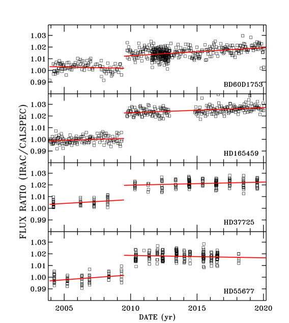
Figure 2: Ratio of our IRAC1 three-pixel radius photometry to the predicted CALSPEC flux for four well observed stars with exposure times of 1.2s, except for HD165459 with 0.2s exposures. This full-frame photometry is binned by AOR to increase the S/N. The red lines are separate linear fits for the cold and warm missions. Only the standard recommended IRAC calibration parameters are included in converting the raw photometry to flux values.

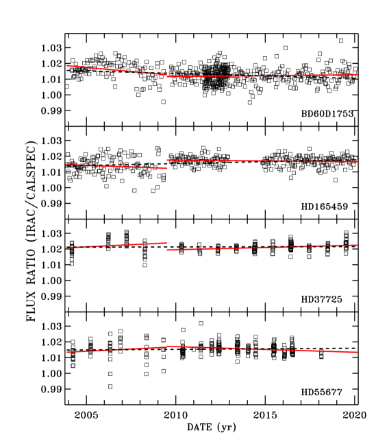
Figure 3: Ratio of our IRAC2 three-pixel radius photometry to the predicted CALSPEC flux for four well observed stars, as in Figure 2. The photometry is binned by AOR to increase the S/N. Only the standard recommended IRAC calibration parameters are included in converting the raw photometry to flux values.

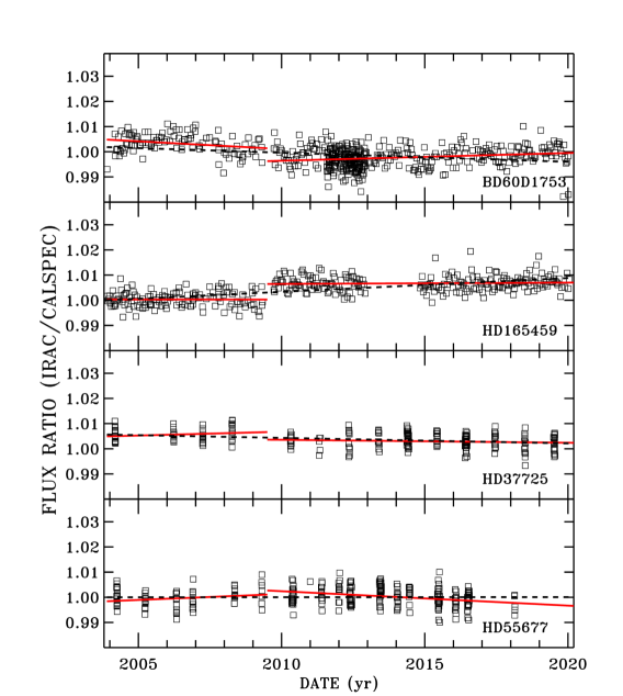
Figure 4: As in Figure 2 after correcting for the discontinuity jump of 1.55% at 2009.5 and for the new IRAC1 time-dependent loss of sensitivity of 0.063 %/yr. The pair of red line fits match the single dashed line fit to $<$0.4%; and the largest deviation from a constant for the dashed lines over the entire 16 years approaches 1% only for HD165459 near 2020.

Table 2 includes the statistics of our red-line linear fits in Figures 2–3, where the slope columns are in %/year. The cold and warm time periods are fit and tabulated separately as slope1 and slope2 for IRAC1–2 in Table 2, while the columns labeled as Jump measure the amount of discontinuity between the fits at 2009.5. The average and uncertainties for the discontinuous jumps at 2009.5 in Figures 2–3 are 1.55 (0.25) and -0.39 (0.20)% for IRAC1–2 with the uncertainties in parentheses. These adjustments are implemented as updates to the warm mission fluxes after 2009.5.

After correcting for the discontinuous jumps and fitting over the complete time period, the average slopes and 1$\sigma$ uncertainties are +0.037 (.020) and -0.010 (.012), for IRAC1–2. Thus, the refined IRAC1 slope value becomes -0.10+0.037=-0.063, while the Krick value of -0.05 for IRAC2 becomes -0.05-0.010=-0.060 %/year. Neither new loss rate differs by more than 2$\sigma$ from the Krick value.

Figure 4 is an example of the results after implementing the new corrections for discontinuities and for the newly derived rates of sensitivity loss. In the worst case of the 0.2s exposures of HD165459, the range of IRAC1 photometry as traced by the dashed line in Figure 4 is 1%, which represents a reduction from the 3% spread in Figure 2 before correction. Section 6.3 discusses the validity of the existing IRAC absolute flux calibration with our adjustments included. The 1% deviation of the dashed line fit from a constant for HD165459 over the whole 2004–2020 period represents an estimate of the systematic uncertainties of our results.

3.5 Repeatability

The rms scatter about the dash-line fits in Figure 4 provide a measure of IRAC repeatability for observations at different epochs and different locations on the detector after making our corrections to the Archival IRAC fluxes. These rms measures range from 0.3–0.4% for IRAC1 and 0.4–0.5% for IRAC2. Thus, 0.3–0.5% reduced by sqrt(N-independent observations binned by AOR) could be included in estimates of the IRAC photometric uncertainty whenever repeatability is a concern. Because these repeatability estimates include some noise sources, repeatability should be improved for cases with higher S/N. However, sub-percent repeatability is already impressive and sets an excellent limit on how precise IRAC results can be with proper photometric corrections and sufficient S/N.

Table 2: Sensitivity Changes

Star	Exp (s)	3.6 µm				4.5 µm
		Slope1	Slope2	Jump(%)		Slope1	Slope2	Jump(%)
BD+60∘1753	1.2	-0.024	+0.069	1.03		-0.114	+0.001	-0.506
HD165459	0.2	+0.036	+0.043	2.18		-0.051	-0.020	+0.126
HD37725	1.2	+0.067	+0.026	1.25		+0.044	+0.018	-0.839
HD55677	1.2	+0.084	-0.020	1.72		+0.047	-0.045	-0.340

3.6 Exposure Time Corrections

Both the IHB and Krick et al. (2021b) point out differences in photometry that depend on exposure time and on subarray vs. full-frame data for channels 1 and 2. Here, a more detailed analysis reveals the photometry dependence on individual exposure times in both subarray and full-frame modes for all four IRAC channels. For the few stars in our sample with robust sets of observations at more than one exposure time, the average flux for each AOR is divided by the average flux at the maximum exposure time for that particular star and channel to form a set of relative flux values as plotted in Figure 5 as small black diamonds. For stars where the maximum exposure time is 0.08 s, those pairs of relative flux at 0.01 and 0.08 s are normalized to the average of all other stars at the exposure level of 0.08 s. The large red diamonds at each exposure time are the averages over all stars for which there are data, where the values of unity at the normalization levels of the maximum exposure times are omitted from the averages.

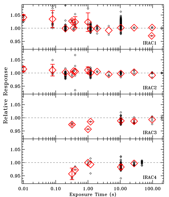
Figure 5: Ratio of our IRAC photometric fluxes to the average IRAC flux for the longest exposure for each star (small black diamonds) for the few stars with robust sets of observations at two or more exposure times. The photometry is binned by AOR to increase the S/N. The large red diamonds are the ratios averaged over the Nstar stars at each measured exposure time from Table 3. The error bars are the $1\sigma$ rms scatter among all the contributing stars and appear for corrections of $\geq 1\%$. The results that are based on only one star have error bars with zero extent. Occasionally, the red diamonds are offset from the centroids of the black points, because the average of all stars is offset from the average of a star with a dominant number of observations.

Table 3: Exposure Time Adjustments

Exposure (s)	Adjustment	rms	Nstar	Ntot
IRAC1
0.01	1.041	0.009	4	2318
0.08	1.035	0.032	4	13069
0.20	0.999	0.004	1	4988
0.32	1.027	0.004	2	1131
0.36	1.001	0.004	2	2071
0.40	1.024	0.020	4	40
1.00	1.023	0.035	4	16
1.20	0.997	0.002	4	4551
1.92	0.999	0.006	2	2386
4.40	0.992	0.023	1	685
10.40	1.002	0.014	4	2842
26.80	1.002	0.001	1	58
93.60	0.971	0.004	1	130
96.80	1.002	0.001	1	36
193.60	1.000	0.004	1	20
IRAC2
0.01	1.015	0.010	2	1068
0.08	1.011	0.022	3	9983
0.20	1.003	0.008	3	5050
0.32	0.995	0.007	2	1132
0.36	1.007	0.001	1	1505
0.40	1.006	0.006	2	20
1.00	1.011	0.012	3	12
1.20	1.000	0.004	5	4735
1.92	1.005	0.005	1	251
4.40	0.995	0.023	1	139
10.40	0.998	0.005	3	294
26.80	1.003	0.008	2	88
96.80	0.991	0.011	1	165
193.60	1.000	0.001	1	20
IRAC3
0.32	0.967	0.013	2	1132
1.00	0.944	0.051	1	4
1.20	0.972	0.033	1	4
10.40	0.985	0.010	4	725
26.80	0.987	0.007	3	108
96.80	0.993	0.010	3	55
193.60	1.000	0.018	3	25
IRAC4
0.32	0.958	0.023	2	1133
0.40	0.973	0.014	1	12
1.00	1.000	0.006	2	8
1.20	0.987	0.028	3	339
10.40	0.983	0.010	4	714
26.80	0.997	0.004	4	118
46.80	1.000	0.001	4	298

Note. — Bold adjustments to derived fluxes are implemented in our data analysis.

Table 3 summarizes the results of the exposure level analysis, where the 13 values in bold represent the corrections that are implemented in the production of final flux values. The adjustment amounts are those $\geq$1% with rms values of less than the adjustment. The correction is in the denominator of the flux calculation. For the 0.08 s exposure time, i.e. 0.1 s frame time, our results are in accord with the elevated normalized flux in figure 3 of Krick et al. (2021b) for IRAC1–2. The other columns in Table 3 are for the rms scatter among the Nstar count of stars with data at that exposure time. For exposure levels with Nstar=1, the rms value is the scatter among the individual AOR measures at that level. Ntot is the total number of useful individual observations in all of the available AORs, where each subarray data set has 64 individual observations. While most of the required adjustments for IRAC1–2 are for the shorter subarray exposures, an exception is the 93.6 s time for IRAC1 at 0.971. In the top panel of Figure 5, the red diamond for the 93.6 s exposure time encompasses the single black square AOR. However, this single AOR includes 130 separate observations of 1743045 and is robust with an rms of only 0.4% among the 130 observations. After making this 3% correction, the average flux for the 93.6 s observations agrees to $<$1% with the average IRAC1 fluxes for 1743045 at five other exposure levels that range from 1.2–193.6 s.

Even though some of our important IRAC 3–4 data have only 0.01 s exposures, our data collection unfortunately includes no observations to calibrate the IRAC3–4 0.01 s exposure level relative to longer times. These average fluxes are arbitrarily assigned an uncertainty of 3%, a typical value for short exposures.

3.7 Saturation

Bright stars with excessive exposure times saturate the IRAC detectors and may produce bad photometry. The IRAC saturation level is defined as 90% of the full-well depth of the detectors, where the full-well depths in electrons for IRAC1–4 from Section 2.3.1 of the IHB are 145000 (110000), 140000 (125000), 170000, and 200000 electrons, respectively, with the warm mission in parentheses. Combining the 90% full-well depths with the sensitivities 770 (840), 890 (730), 420, and 910 (electrons/sec)/(mJy) from the IHB Table 2.4 and the percent signal in the peak pixel of 42 (37), 43 (34), 29, and 22 from the IHB Table 2.1 provides the IRAC1–4 saturation limits in (mJy s) of 404 (319), 329 (453), 1256, and 899. Dividing these (mJy s) limits by the predicted flux from the CALSPEC SED in mJy from Equations 1 and 5, yields the exposure time to saturation for each band.

An alternative, set of (mJy s) limits accrue from multiplying the exposure time by the IHB Table 2.11 tabulated maximum unsaturated point source flux in mJy, as calculated from the IHB equation 2.14. For example for IRAC1, these alternative limits range from 190–368 (192–288) in comparison to the above 404 (319). Even though puzzling to the neophyte, the IHB suggests that the saturation limits depend on frame time, instead of exposure time; and saturation limits in frame time multiplied by tabulated maximum unsaturated point source flux in mJy are much closer to our 404 (319), ie. 379–400 (280–460). There is still a lot of scatter but the values agree much better with our estimates. Another example compares our IRAC4 (mJy s) limit of $\approx$900 to the IHB range of 450–5420 for exposure time or 900–5600 for frame time. Because the IHB includes the effects of the background current that contributes to the filling of the detector well capacity, the saturation limits should be less, NOT more than our 900 that ignores the background contribution. Because of the ambiguities associated with Table 2.11 plus the omission of some important exposure times, like 1.0 and 46.8 s, our simple-minded estimates define our saturation levels. Any adjustments to our values would just affect the rare inclusion or exclusion of small bits of data in the measured IRAC fluxes.

The 46,122 IRAC1 and 44,145 IRAC2 observations for HD165459 cover a wide range from under- to overexposure. For the predicted IRAC1–2 fluxes of 643, 416 mJy, the saturation limits to 90% full-well depth of the peak pixel are IRAC1 0.63s (0.50s) and IRAC2 0.79s (1.09s). Table 4 illustrates the measured fluxes from minimum to the maximum exposure time, where a blank row separates the saturated from the unsaturated data. For the saturated data, a correction for saturation is required, so the saturated flux measures utilize the _cbcd.fits files. The unsaturated flux measures in Table 4 and the robust values for the longest exposures in the last row all agree to 2% for both IRAC1 and IRAC2. These long exposures of 23.6 and 26.8 s have overexposure factors of 37 (47) and 34 (25) for each channel with the warm mission in parentheses.

All the measured photometric flux values in Table 5 utilize only unsaturated IRAC data, except for $\eta$ UMa, which has only saturated data. The overexposure levels for the existing 10.4s exposures for all channels 1–4 have overexposure factors between 780 and 77 and enable accurate photometry for $\eta$ UMa from the *cbcd.fits files. However, an additional uncertainty of 2% is included for the $\eta$ UMa fluxes because of possible systematic errors in the use of saturated data.

In Table 5, Unc is the 1$\sigma$ uncertainty, N is the total number of observations used to find the average Flux, and Ratio is IRAC photometry divided by CALSPEC synthetic photometry. Except for the few arbitrary estimates of systematic uncertainty, Usys, assigned for variability, saturation in $\eta$ UMa, or lack of correction for the IRAC3–4 short exposure times, the uncertainties are just statistical. The statistical contributions arise from Uobs, the rms scatter among the observations used to measure the flux as divided by the square root of the number observations, N, and from Uoff, the total range of the set of five photometry values with the 0.2″ offsets. The final uncertainty estimates are $sqrt(Uobs^{2}+Uoff^{2}+Usys^{2})$. In general, Uobs is negligible in comparison to Uoff, except for the cases with less than $\approx$10 observations, while most cases have Usys=0. Many of these error estimates seem too low, possibly because of unidentified systematic errors, such as errors in the IRAC system fractional throughput and such as possible non-linearity for weak exposures, where only a small fraction of the detector full-well capacity is filled.

IRAC exposures with exposure times less than a factor of 14 below the maximum unsaturated exposure contribute only noise and are not included in our analyses. In order to include the 2257 faint 0.01 s exposures and augment the three unsaturated 0.20s exposures, the acceptance level is

Table 4: HD165459 Flux vs. Exposure Time

Frame time (s)	Exptim (s)	3.6 µm					4.5 µm
		Flux (mJy)	Unc (%)	N	Ratio		Flux (mJy)	Unc (%)	N	Ratio
0.02	0.01	644.0	0.63	1316	0.996		421.0	0.37	817	0.993
0.10	0.08	631.8	2.27	4300	0.977		423.8	0.66	2381	1.000
0.40	0.20	646.1	0.73	3500	0.999		422.4	0.12	3394	0.997
0.40	0.32	644.6	0.23	252	0.997		419.2	0.20	252	0.989
0.40	0.36	646.5	1.15	32423	1.000		423.7	0.28	32908	1.000
2	1.20	520.8	4.54	8	0.806		415.9	0.12	601	0.982
6	4.40	697.0	2.32	9	1.078		428.2	1.50	9	1.011
12	10.4	681.3	2.99	9	1.054		431.7	1.02	9	1.019
30	23.6,26.8	656.7	0.41	98	1.016		427.6	0.36	101	1.009

Note. — Unc is the 1$\sigma$ uncertainty, N is the number of observations used, and Ratio is the flux normalized to the flux for the 0.36 s exposures.

relaxed from a factor of 14 to 20 below 0.20s for HD14943 IRAC2.

Table 5: Measured IRAC Fluxes

Star	3.6 µm				4.5 µm				5.8 µm				8.0 µm
	Flux	Unc	N	Ratio	Flux	Unc	N	Ratio	Flux	Unc	N	Ratio	Flux	Unc	N	Ratio
	mJy	%			mJy	%			mJy	%			mJy	%
	HOT Stars
10LAC	1.578e+03	2.71	63	0.997	1.010e+03	1.32	63	1.011	6.165e+02	3.29	63	0.991	3.276e+02	3.22	63	0.972
ETAUMA	2.955e+04	2.22	10	0.975	1.934e+04	2.09	10	1.000	1.267e+04	2.80	10	1.039	6.588e+03	2.26	10	0.983
G191B2B	1.999e+00	0.61	113	0.992	1.283e+00	0.57	63	1.005	8.081e-01	1.17	58	1.009	4.351e-01	2.85	37	0.986
GD153	4.864e-01	0.68	108	0.986	3.097e-01	0.50	82	0.993	1.937e-01	4.91	59	0.992	1.082e-01	7.23	62	1.009
GD71	6.714e-01	0.73	60	0.994	4.355e-01	0.66	69	1.026	2.763e-01	3.27	59	1.042	1.608e-01	5.22	64	1.112
LAMLEP	2.431e+03	0.69	2325	0.995	1.567e+03	0.20	2320	1.014	9.481e+02	3.14	63	0.980	5.148e+02	3.29	63	0.975
MUCOL	1.003e+03	1.04	2202	0.993	6.565e+02	0.19	2263	1.031
	A Stars
109VIR	9.297e+03	0.83	7413	0.998	6.219e+03	0.21	2506	1.033
1732526*	3.486e+00	1.66	51	0.975
1743045	2.066e+00	2.60	244	1.020	1.343e+00	1.16	247	1.022	8.757e-01	0.48	116	1.043	4.908e-01	0.63	370	1.052
1757132	9.436e+00	0.44	155	1.014	6.216e+00	0.21	95	1.030	4.023e+00	0.36	35	1.044	2.214e+00	0.50	107	1.036
1802271	5.053e+00	0.71	101	1.007	3.300e+00	0.15	112	1.017	2.114e+00	0.41	48	1.020	1.173e+00	0.49	158	1.021
1805292	4.398e+00	0.84	52	1.002	2.941e+00	0.47	33	1.035
1808347*	6.524e+00	3.40	1782	0.997	4.339e+00	1.51	23	1.023
1812095*	8.496e+00	2.36	3171	1.002	5.643e+00	1.50	2293	1.027	3.624e+00	1.52	590	1.033	1.990e+00	1.57	482	1.024
BD60D1753	3.869e+01	2.12	5626	0.992	2.548e+01	0.81	4705	1.011	1.636e+01	0.26	519	1.018	9.103e+00	0.44	528	1.023
DELUMI	5.416e+03	1.07	252	0.981	3.598e+03	0.48	250	1.007
ETA1DOR	1.362e+03	0.57	743	0.992	8.891e+02	0.25	503	1.004	5.665e+02	0.20	252	1.005	3.188e+02	0.57	250	1.023
HD101452	5.180e+02	1.20	5	1.021	3.391e+02	0.65	4	1.031	2.158e+02	0.36	5	1.027	1.212e+02	0.68	4	1.042
HD116405	1.122e+02	0.60	10	0.996	7.330e+01	0.59	8	1.011	4.652e+01	0.41	5	1.010	2.601e+01	0.59	4	1.022
HD128998	1.303e+03	0.34	1045	0.987	8.690e+02	0.55	756	1.019	5.460e+02	0.26	566	1.005	3.085e+02	0.56	566	1.025
HD14943	1.799e+03	0.79	2264	1.001	1.191e+03	0.08	2259	1.024	7.597e+02	0.27	3	1.023	4.271e+02	0.72	3	1.038
HD158485	9.702e+02	0.50	484	0.999	6.458e+02	0.39	252	1.027	4.057e+02	0.21	252	1.011	2.307e+02	0.55	251	1.037
HD163466	7.949e+02	0.33	862	1.002	5.307e+02	0.18	848	1.033	3.377e+02	0.22	567	1.028	1.895e+02	0.82	564	1.040
HD165459	6.461e+02	1.09	38607	1.004	4.236e+02	0.27	38752	1.019	2.650e+02	0.24	11080	0.999	1.507e+02	0.46	1125	1.026
HD180609	6.382e+01	0.59	792	1.007	4.176e+01	0.99	1407	1.017	2.693e+01	0.24	110	1.027	1.528e+01	0.46	522	1.051
HD2811	4.216e+02	1.34	5	1.011	2.751e+02	0.64	4	1.018	1.760e+02	0.53	5	1.020	9.916e+01	0.88	4	1.035
HD37725	1.895e+02	0.75	2060	1.004	1.248e+02	0.28	1856	1.021	8.053e+01	0.24	266	1.032	4.572e+01	0.53	244	1.059
HD55677	6.005e+01	0.83	2692	1.000	3.954e+01	0.17	2447	1.015	2.528e+01	0.25	305	1.016	1.418e+01	0.48	298	1.028
	G Stars
16CYGB	3.716e+03	2.52	63	0.952									8.981e+02	0.45	4	0.995
18SCO	7.032e+03	1.22	251	0.929
HD106252	1.168e+03	1.68	4773	0.978	7.392e+02	0.67	250	0.967					2.635e+02	3.14	251	0.955
HD159222	2.633e+03	1.13	4768	0.961	1.697e+03	0.14	251	0.972					5.973e+02	3.26	251	0.944
HD205905	2.101e+03	0.47	250	0.955	1.353e+03	0.45	251	0.962					4.782e+02	3.11	252	0.941
HD37962	8.536e+02	0.94	252	0.962	5.469e+02	0.60	252	0.963					1.963e+02	3.20	252	0.955
HD38949*	7.486e+02	1.68	250	0.963	4.843e+02	1.58	252	0.969					1.722e+02	4.73	250	0.961
P330E	7.609e+00	0.77	62	1.002	4.994e+00	0.31	8	1.025	3.179e+00	0.54	5	1.014	1.747e+00	4.33	4	0.997

Note. — * Indicatates variability, see Section 5. Column 1 is the CALSPEC name, Unc is the 1$\sigma$ uncertainty, N is the number of observations used, and Ratio is the ratio of the IRAC Flux (mJy) to the CALSPEC synthetic photometry.

4 New NLTE Model SEDs for OB Stars

For this paper, Hubeny has updated the OB NLTE model SED grids of Lanz & Hubeny (2003, 2007) using a more complete hydrogen atom to produce more realistic IR flux predictions. In particular, the new NLTE spectra have a much better description of line confluences and of the contribution to the opacity in very high series members. In addition, there are improvements in the treatment of the hydrogen and He II continua from high levels, inclusion of more scattering opacity sources, and updates to the physics of level dissolution. Each model has 29957 points at constant spectral resolution of R=5000 and a micro-turbulent velocity of 2 km/s. The Asplund et al. (2009) element abundances are used for computing the spectra.

The improvements in the physical description of hydrogen line profiles, level dissolution, and the treatment of pseudo-continua influence the overall atmospheric structure and the emergent spectrum. However, because the most significant improvements occur for hydrogen lines in the infrared region, where the flux for O and B stars is low, these changes do not cause significant changes in the global model structure. Typically, the relative difference in the continuum level amounts at most to a few times 0.1%.

This finding permits a simplified computational strategy, using the model atmosphere structure of temperature, electron density, and atomic level populations from published OSTAR2002 and BSTAR2006 grids to merely recompute emergent spectra with SYNSPEC for all available models, which is several orders of magnitude less time-consuming than to recompute full NLTE metal line-blanketed model atmospheres as was done in Lanz & Hubeny (2003, 2007).

See Hubeny et al. (2021) for a description of the most recent versions of tlusty and SYNSPEC. The new OB grid is available in the Mikulski Archive for Space Telescopes (MAST) as a High Level Science Product via 10.17909/bsbk-pj11 (catalog 10.17909/bsbk-pj11). The grid contain 1082 model pairs of spectra and continua and covers effective temperature ($T_{\mathrm{eff}}$) in the range 15,000–55,000 K and surface gravity ($\log g$) between 1.75 and 4.75, with steps of 0.25, where g has units of $cm~{}s^{-2}$. The steps in $T_{\mathrm{eff}}$ are 1,000 K between 15,000 and 29,000 K and 2,500 K between 30,000 and 55,000 K. As $T_{\mathrm{eff}}$ rises, more of the unstable lower surface gravities are omitted. There are five metallicity values ($\log Z$)=[M/H] of 0.301, 0.000, -0.301, -0.70, and -1.00, which correspond to Z=2, 1, 0.5, 0.2, and 0.1, where Z=1 is the solar value.

5 Variability and Rejected CALSPEC Stars

TESS data indicate variability in four CALSPEC standards (Mullally et al., 2022), which vary by more than a peak-to-peak limit of 0.5% and are flagged with an asterisk in Table 5. These stars and the amount of variability (%) in parentheses are 1732526 (1.40), 1808347 (1.65), 1812095 (1.57), and HD38949 (1.17). Such low levels of variability do not seriously affect our results, partly because of averaging over time and partly because none of the four stars display anomalous flux levels. However, an extra 1.5% is included in their uncertainty estimates.

C26202 (a.k.a. 2MJ03323287) is faint and in a crowded field, which makes its photometry too unreliable to include. WD0308-565 was considered for addition to the work of Krick et al. (2021a) but is rejected as too faint to provide reliable IRAC photometry. LDS749B and WD1057+719 are even fainter than WD0308-565 and are not reported here, even though LDS749B IRAC1 with a 4.6% $1\sigma$ uncertainty happens to fall within 1% of its model. Sirius is an important CALSPEC star (Price et al., 2004; Bohlin et al., 2020), but the Spitzer Archive contains no observations which produce straightforward flux values.

6 Results

6.1 Comparisons among the Three Spectral Categories

Figure 6 shows the ratio of our Spitzer IRAC photometry from Equation (5) to the synthetic CALSPEC photometry from Equation (1) for our three categories of stars (Gordon et al., 2022). Purple symbols identify the IRAC photometry that has an uncertainty of $>$3%. In the top panel for our hot-star category, the three primary CALSPEC standards (red) agree with IRAC within $2\sigma$, except for GD71 at 4.5 µm, where that IRAC2 is 2.6% ($3.9\sigma$) high. The IRAC3-4 data for the bright 10Lac and $\lambda$ Lep with green connecting lines fall significantly below unity and are purple because of the extra 3% uncertainty assigned to these short 0.01 s exposures, which have no available correction in Table 3 but are likely to be systematically low, as suggested by the trends for IRAC3–4 in Table 3. The IRAC3 for $\eta$ UMa is 3.6% high but that is only $1.3\sigma$.

In the middle panel for the A-type stars, the ratios for all IRAC filters clump tightly and suggest a rising trend from short to long wavelength. One explanation for this trend could be that the CALSPEC models for A-stars are systematically too dim as the wavelength increases from 3.6 to 8 µm. Perhaps, the LTE A-star models used for the CALSPEC SEDs should have more of a rising slope from 3.6 to 8 µm, as suggested by the NLTE discussion below for the OB-stars. Alternatively, contamination by a range of contributions by hot dust to the A-star IR fluxes seems unlikely, because the rms scatter among the IRAC/CALSPEC A-star ratios from IRAC1 to IRAC4 does not increase above 1.3% in Table 6.

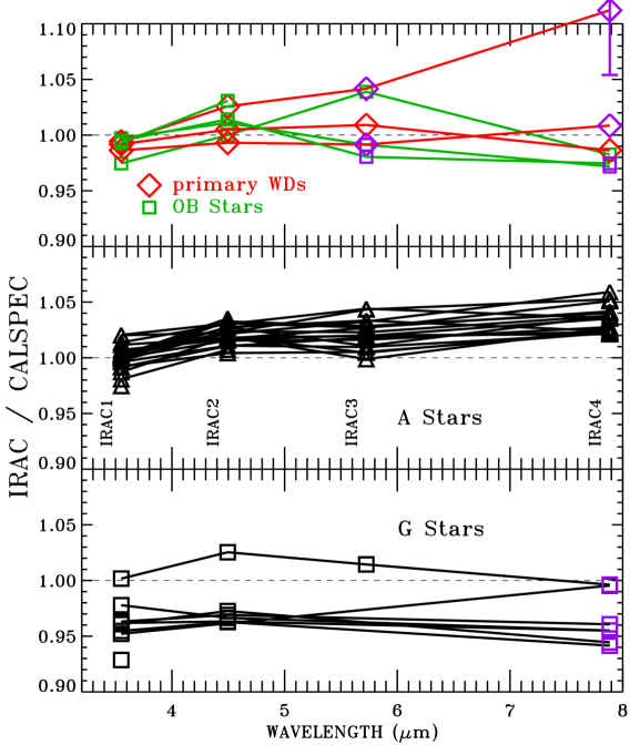
Figure 6: Ratio of photometry in the four Spitzer IRAC bands to synthetic photometry of CALSPEC SEDs, where the synthetic photometry is from models normalized to the STIS fluxes at 6800–7700 Å. There are three panels for the three different categories of JWST flux standards, i.e. the G-type stars, the A-stars, and the hot WDs plus OB-stars. The model IR extentions of the OB CALSPEC standards are updated with the new NLTE model grid. Purple symbols flag points with $>$3% IRAC uncertainties. A $1\sigma$ error bar appears for the most extreme point that lies more than 10% from unity to demonstrate that the ratio is still within $2\sigma$ of unity.

Table 6: IRAC / CALSPEC

Channel	Star Set	IRAC/CALSPEC	rms	N
IRAC1	Prime WDs	0.991	0.004	3
IRAC2	Prime WDs	1.005	0.016	3
IRAC3	Prime WDs	1.012	0.025	3
IRAC4	Prime WDs	1.010	0.066	3
IRAC1	A	1.000	0.011	22
IRAC2	A	1.022	0.009	21
IRAC3	A	1.018	0.013	17
IRAC4	A	1.034	0.011	17
IRAC1	G	0.963	0.022	8
IRAC2	G	0.978	0.025	6
IRAC3	G	1.014		1
IRAC4	G	0.991	0.023	7

In the bottom panel for the G stars, there is only one IRAC3 measure and most of the IRAC4 points have large uncertainty, so not much can be concluded regarding the averages for IRAC3-4. The five low values of the seven IRAC4 points have have only 0.01 s exposures, so are probably systematically low like the O-stars 10Lac and $\lambda$ Lep, while 16CygB and P3303 are near unity with their longer exposure times of 1 and 26.8 s, respectively. While the main clump of IRAC1-2 G-star points are robust and low by 2–7%, P330E lies high by 3–4% with uncertainties as low as $1\sigma$=0.31% for IRAC2. The P330E ratios with exposure times of 10.4s are consistent with the A-star locus, while all 12 of the low IRAC1–2 G-star points are entirely from 0.01 s exposures. However, for stars hotter than G, there are 10 IRAC1–2 photometry values dominated by 0.01 s exposures; and none of these 10 have IRAC fluxes as low as the G-star IRAC/CALSPEC weighted averages of 0.963 and 0.978 for IRAC1 and IRAC2, respectively, from Table 6. In particular, the hotter star 0.01 s ratios range from 0.981–1.001 for IRAC1 and 1.007–1.033 for IRAC3. Furthermore, non-linearities cannot cause the G-stars to have low fluxes, because the detector full-wells are filled to similar depths of a few percent for all 22 of the 0.01 s exposure times from all three categories of stellar type.

Thus, the possibility seems unlikely that all of the G-star IRAC1–2 0.01 exposures are erroneous. A likely explanation for the low IRAC/CALSPEC ratios for many G-stars is an inadequate STIS spectral range of only 0.3–1 µm for fitting models, while P330E has WFC3 and NICMOS data extending to 2.5 µm to better constrain its fit. In figure 4 of Bohlin et al. (2017), the fits in the IRAC wavelength range to STIS alone for G-stars tend to lie above the fits to STIS+NICMOS by up to $\approx$3% for P330E. A WFC3 IR grism campaign to measure the 1–1.7 µm SEDs of the seven deficient G-stars should be done to provide more reliable models for predicting fluxes longward of 2 µm.

Table 6 summarizes the results, where the hot-star category includes only the three primary WDs. Small offset in IRAC/CALSPEC fluxes for any group of stars is not surprising, as the uncertainties of both the CALSPEC and the IRAC flux calibrations are of order 2%. However, the systematically rising offsets from zero at 3.6 µm to 3% at 8 µm  for the A-star group differ from the hot-star group. That systematic difference cannot be caused by an IRAC flux calibration error, as the same IRAC calibration is applied in the same way for all three groups. To make the A-star models agree with the IRAC data, the required amount of brightening at 8 µm relative to 3.6 µm is $\approx$3% for the LTE BOSZ models (Bohlin et al., 2017) used to extend the HST/CALSPEC fluxes to IRAC wavelengths. Alternatively, the IRAC data for the three faint primary WDs relative to the generally brighter ensemble of A-stars is in error; or the well-vetted models for the primary WDs (Bohlin et al., 2020) are erroneous. However, there is a small possibility that the WD/A-star offsets are mostly statistical, even though all four WD ratios lie below the corresponding weighted average A-star ratio. Non-linearity seems an unlikely cause of the WD vs. A-star problem, because the brightest WD G191B2B has nearly the same flux level as the faintest A-star 1743045. None of the four G191B2B IRAC photometry results exceeds its model by more than 0.6% but 1743045 is among the highest A-stars at 3–6% above its LTE BOSZ model.

6.2 Comparisons with the SEDs of the Hot Stars

Figure 7 compares the IRAC photometry to CALSPEC SEDs for the hot stars in the top panel of Figure 6, where the IRAC data (triangles) are plotted at their pivot-wavelengths and their deviations from the red and green SEDs are the same as the deviation from unity in Figure 6.

While the blue curves are the LTE BOSZ models fit to the STIS data at 6800–7700 Å for the three OB-stars and are the current versions in CALSPEC, the green curves are the same fits but using our new NLTE OB-star grid and have similar reduced $\chi^{2}$. The biggest difference in reduced $\chi^{2}$ is for 10 Lac with 4.0 and 2.8 for the NLTE and BOSZ residuals, respectively. Because the three IRAC1 points are closer to the green NLTE models and all three IRAC2 points are much closer to the NLTE models, the green NLTE models are a much better match to the reliable IRAC1–2 fluxes; and NLTE versions stis_006 and will replace the stis_005 versions of LTE models in CALSPEC. Hot WD models show a similar effect for the IR flux of the G191B2B NLTE model, which rises from agreement with an LTE model at 1 µm to $\approx$10% higher at 8 µm in figure 3 of Bohlin et al. (2011).

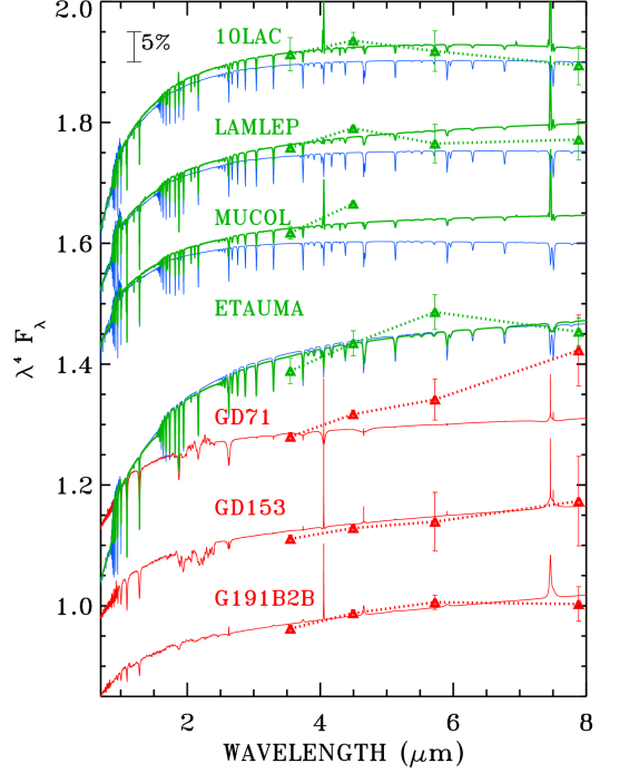
Figure 7: The SEDs scaled by $\lambda^{4}$ and then scaled to unity near 6 µm for the seven stars in the top panel of Figure 6, using the LTE models for OB-stars (blue). Each star above G191B2B is offset by 0.15 in Y. The green SEDs are the new NLTE models matched to the blue LTE models at 6800–7700 Å. The red SEDs are the three primary WDs from CALSPEC, as specified in Bohlin et al. (2020). Triangles illustrate the difference between our IRAC photometry and CALSPEC at the four IRAC pivot wavelengths. The most reliable IRAC1-2 photometry agrees much better with the NLTE models (green) than with the LTE models (blue) for the three stars at the top.

6.3 Absolute Flux Calibration on the CALSPEC Scale

Table 6 summarizes the weighted average results for the three categories of stars, where only the three fundamental primary WDs are included for the hot star category. These three primary WDs form the basis of the HST/CALSPEC absolute flux system; and the agreement with the existing IRAC flux calibration is, perhaps, fortuitous because of our adjustments to the subarray aperture corrections, our adjustments to the IRAC sensitivity changes with time in Table 2, and our revision of the exposure times in Table 3. However, these differences are minor in many cases, e.g. our flux values in Table 5 agree to a maximum difference of 3% for G191B2B IRAC4 among the eight measures of the three prime WDs reported by Krick et al. (2021a). Furthermore, the good agreement of the four OB-stars in Figure 7 with their green model curves reinforces the WD results, especially for IRAC1–2.

The Table 6 results for the three prime WDs demonstate agreement between the IRAC and CALSPEC fluxes within 1% for all four IRAC channels when using the existing flux calibration of Carey et al. (2012). The most significant difference is 0.991, i.e. 0.9%, with an rms uncertainty of 0.004, i.e. 0.4%. This 0.9% offset is only 2.3$\sigma$ and does not justify a revision to the existing IRAC flux calibration.

6.4 Comparison with the Krick et al. (2021a) Fluxes

There is good agreement of our Table 5 with the eight Krick et al. (2021a) values for the three primary WDs, but Krick does not report IRAC3–4 values for GD153 or GD71. Again in the hot star category, the results are similar for the three OB stars 10 Lac, $\lambda$ Lep, and $\mu$ Col, while Krick does not include the saturated $\eta$ UMa. For the A-stars, the biggest difference with our Table 6 is 2% for IRAC1 for 18 stars, while our total star count is 22. For the G-stars, Krick gets better agreement with the models for IRAC1–2, but worse agreement and larger scatter for IRAC4. For P330E, both sets of average fluxes agree to $<$2%, except for IRAC4, where the Krick value is 9% larger than our Table 5 value that agrees with the P330E model. The set of eight G-stars is the same for both analyses.

6.5 Fitting Models with IRAC Fluxes

Could the overall model fits be improved by adding the IRAC constraints to the HST fluxes and then refitting to get new models? For the A-stars, the new fits change by no more than $\approx$1%, which validates the fitting to the HST SEDs only. However, for the G-stars, major changes result with the discovery that there are models that fit both the HST and IRAC fluxes nearly perfectly, i.e. typically within 1% on average. These fits seem wonderful at first glance, but upon close examination, the resulting reddening, E(B-V) extinctions, are unreasonably large. For example, the G2V star 18 Sco has a (B-V)=0.65 for an expected E(B-V)=0.02 mag. However, the model fit to the STIS+IRAC fluxes requires E(B-V)=0.10, i.e. a 0.08 mag discrepancy compared to the usual expected photometry errors of 0.01–0.02 mag. A resolution of this problem will come from JWST measures of A-star/G-star brightness ratios. If these JWST ratios agree with both of the same ratios for STIS in the 0.8–1 µm range and for IRAC, then the insufficiently constrained G-star models must have the wrong shape over this wavelength range. Because of this G-star quandary, achieving the small gains from using the IRAC data to constrain just the hotter star models seems to be an unworthy exercise.

7 Conclusions

Table 6 demonstrates agreement to $\approx$1% between IRAC and CALSPEC for the three primary WD standard stars G191B2B, GD153, and GD71. Similarly, the average differences for four hot OB stars confirm the WD results to 2% for IRAC1–3. The average results for the robust set of 17–22 A-stars show agreement with the hotter star results for IRAC1 but are discrepant by as much as 3.4% at IRAC4. In the 4.5–8 µm wavelength region, the 2–3% A-star offsets from the WD ratios of IRAC/CALSPEC define the uncertainties of the current CALSPEC hot star SEDs with respect to the A-star category. For the G-star category, the set of data for IRAC3–4 lacks sufficient precision, while most of the IRAC1–2 G-star ratios to CALSPEC are discrepant with the hotter star ratios. However, one star P330E with WFC3 spectrophotometry to 1.7 µm and NICMOS data to 2.5 µm agrees with the A-star results. The other seven G-stars have only STIS data that exend to just 1 µm. When fitting P330E using just the STIS data, the fitted model in the IRAC wavelength range is $\approx$3% above the model fitted to the full range to 2.5 µm. Thus, a major contributor to the IRAC/CALSPEC G-star discrepancy is inadequate spectral coverage for fitting models, which makes the models systematically too bright by up to 4% in Table 6. The G-star STIS spectra cover only 0.3–1 µm in comparison to a minimum range of 0.17–1 µm for hotter stars. Therefore, the current CALSPEC model extensions for the seven G-stars with little flux below 0.3 µm and no constraining HST data longward of 1 µm are likely to be a few percent too high in the IRAC wavelength range.

In summary, there is no strong evidence from the IRAC data for problems with the spectral grids used for predicting the IR SEDs. Inadequacies of the observational data both from HST and Spitzer contribute to deviation of the models from the IRAC photometry. To be conservative, uncertainties of 2, 3, 4% longward of 3 µm should be adopted for our hot-star, A star, and G star categories, respectively. JWST measures of hot-stars with respect to the A and G stars can be used to correct the cooler star models and reduce their uncertainty relative to the more accurate hot-star category.

References

- Asplund et al. (2009) Asplund, M., Grevesse, N., Sauval, A. J., & Scott, P. 2009, ARA&A, 47, 481
- Bohlin (2014) Bohlin, R. C. 2014, AJ, 147, 127
- Bohlin et al. (2014) Bohlin, R. C., Gordon, K. D., & Tremblay, P.-E. 2014, PASP, 126, 711
- Bohlin et al. (2020) Bohlin, R. C., Hubeny, I., & Rauch, T. 2020, AJ, 160, 21
- Bohlin et al. (2017) Bohlin, R. C., Mészáros, S., Fleming, S. W., et al. 2017, AJ, 153, 234
- Bohlin et al. (2011) Bohlin, R. C., Gordon, K. D., Rieke, G. H., et al. 2011, AJ, 141, 173
- Carey et al. (2012) Carey, S., Ingalls, J., Hora, J., et al. 2012, in Society of Photo-Optical Instrumentation Engineers (SPIE) Conference Series, Vol. 8442, Space Telescopes and Instrumentation 2012: Optical, Infrared, and Millimeter Wave, ed. M. C. Clampin, G. G. Fazio, H. A. MacEwen, & J. Oschmann, Jacobus M., 84421Z
- Fazio et al. (2004) Fazio, G. G., Hora, J. L., Allen, L. E., et al. 2004, ApJS, 154, 10
- Gordon et al. (2022) Gordon, K. D., Bohlin, R., Sloan, G. C., et al. 2022, The James Webb Space Telescope Absolute Flux Calibration. I. Program Design and Calibrator Stars, doi:10.48550/ARXIV.2204.06500
- Hubeny et al. (2021) Hubeny, I., Allende Prieto, C., Osorio, Y., & Lanz, T. 2021, arXiv e-prints, arXiv:2104.02829
- Kovtyukh et al. (2003) Kovtyukh, V. V., Soubiran, C., Belik, S. I., & Gorlova, N. I. 2003, A&A, 411, 559
- Krick et al. (2016) Krick, J. E., Ingalls, J., Carey, S., et al. 2016, ApJ, 824, 27
- Krick et al. (2021a) Krick, J. E., Lowrance, P., Carey, S., et al. 2021a, AJ, 161, 177
- Krick et al. (2021b) Krick, J. E., Lowrance, P. J., Carey, S., et al. 2021b, Journal of Astronomical Telescopes, Instruments, and Systems, 7, 038006
- Lanz & Hubeny (2003) Lanz, T., & Hubeny, I. 2003, ApJS, 146, 417
- Lanz & Hubeny (2007) —. 2007, ApJS, 169, 83
- Mullally et al. (2022) Mullally, S. E., Sloan, G. C., Hermes, J. J., et al. 2022, arXiv e-prints, arXiv:2201.03670
- Price et al. (2004) Price, S. D., Paxson, C., Engelke, C., & Murdock, T. L. 2004, AJ, 128, 889
- Scolnic et al. (2014) Scolnic, D., Rest, A., Riess, A., et al. 2014, ApJ, 795, 45
- Stubbs & Brown (2015) Stubbs, C. W., & Brown, Y. J. 2015, Modern Physics Letters A, 30, 1530030
- Tayar et al. (2020) Tayar, J., Claytor, Z. R., Huber, D., & van Saders, J. 2020, arXiv e-prints, arXiv:2012.07957