Semi-Parametric Contextual Bandits with Graph-Laplacian Regularization

Abstract

Non-stationarity is ubiquitous in human behavior and addressing it in the contextual bandits is challenging. Several works have addressed the problem by investigating semi-parametric contextual bandits and warned that ignoring non-stationarity could harm performances. Another prevalent human behavior is social interaction which has become available in a form of a social network or graph structure. As a result, graph-based contextual bandits have received much attention. In this paper, we propose SemiGraphTS, a novel contextual Thompson-sampling algorithm for a graph-based semi-parametric reward model. Our algorithm is the first to be proposed in this setting. We derive an upper bound of the cumulative regret that can be expressed as a multiple of a factor depending on the graph structure and the order for the semi-parametric model without a graph. We evaluate the proposed and existing algorithms via simulation and real data example.

1 Introduction

In contextual multi-armed bandits (MAB), a learning agent sequentially chooses actions while balancing to maximize the reward (exploitation) and to learn the reward mechanism as a function of contexts with higher precision (exploration). Algorithms for contextual MAB problems have demonstrated their usefulness in many applications including recommendations of news articles, advertisements, or behavioral interventions (Li2010a; Tang2013; Tewari2017a). Thompson sampling (TS)-based algorithms randomly choose an action from repeatedly updated posterior, and have been widely used among other bandit algorithms (Scott2010; Kaufmann2012; Agrawal2013).

The semi-parametric contextual bandit (Greenewald2017; Krishnamurthy2018; Kim2019) models the mean of the reward by a linear function of the contexts and a time-varying intercept. The algorithms for semi-parametric models allow the reward distribution to change over time in a non-stationary manner. For example, behavior may change over time depending on the user’s circumstances or preference for a shopping item may change according to a time trend. These may not be captured in the context vectors. In the single-user setting, the semi-parametric bandits have demonstrated success in accommodating non-stationarity in mobile health and product recommendation (Greenewald2017; Kim2019; Peng2019; Liao2019).

In many real-life settings, there are multiple users and the relationships among the users in a social network are often available as side information. Such graph information has been utilized in recommendation (Li2010a; Delporte2013; Rao2015). Several graph-based contextual MAB algorithms have been proposed to take the graph information into account under the ordinary linear reward assumption (Casa-bianchi2013; Gentile2014; Vaswani2017; Li2019; Yang2020). The aforementioned graph-based methods have shown to take advantages of a graph structure and perform well, but may be restrictive in real-life settings when the rewards tend to change over time.

Our goal is to construct a semi-parametric bandit algorithm that accommodates multiple users equipped with a network, with practically feasible computational cost. To the best of our knowledge, our algorithm is the first algorithm proposed in this setting. The main contributions of the work presented in this paper are as follows.

• We propose SemiGraphTS (semi-parametric-graph-Thompson-sampling), a novel TS algorithm for a setting in which each user’s reward follows the semi-parametric model and user-specific parameters are regularized by the given graph.

• We derive an upper bound of the cumulative regret for SemiGraphTS, which be expressed as a multiple of a factor depending on the graph structure and the bound from the semi-parametric model without a graph.

• We propose a novel scalable estimator for the user-specific parameter that incorporates the estimators from the neighbors defined by the graph structure while conditioning out time-dependent coefficients. This plays a crucial role in building the SemiGraphTS algorithm. We establish a high-probability upper bound for its estimation error.

2 Model and problem setting

We study the semi-parametric contextual bandit problem for multiple users equipped with a user network. Suppose that there are $n$ users, say $j\in V=\{1,\ldots,n\}$. For each time step $t=1,\ldots,T$, the learning agent is instructed which user to serve, say $j_{t}$. The agent is supposed to recommend an item or pull an arm for the target user based on the previous action history and the contexts describing the items. Suppose that there are $N$ candidate arms, say $i=1,\ldots,N$, and that a context vector $b_{i}(t)\in\mathbb{R}^{d}$ represents the feature of the $i$-th item at time $t$. We denote by $a(t)$ the selected arm to recommend to the target user. We let $r_{i,j}(t)$ be the reward for arm $i$, user $j$ at time $t$. Upon the action, the user returns a user-specific reward for the chosen arm, say $r_{a(t),j_{t}}(t)$. The information given to the learner at time $t$ is formally described as filtration $\mathcal{F}_{t-1}=\{j_{t},\{b_{i}(t)\}_{i=1}^{N}\}\bigcup\left(\bigcup_{\tau=1}^{t-1}\{j_{\tau},\{b_{i}(\tau)\}_{i=1}^{N},a({\tau}),r_{a(\tau),j_{\tau}}(\tau)\}\right)$.

The multiple-user semi-parametric reward model is described as below:

$$r_{i,j}(t)=\nu_{j}(t)+b_{i}(t)^{T}\mu_{j}+\eta_{i,j}(t),$$ (1)

for $i=1,\ldots,N$, $j=1,\ldots,n$, and $t=1,\ldots,T$. Here, $\mu_{j}\in\mathbb{R}^{d}$ denotes the unknown user-specific parameter that represents the preference of the $j$-th user for a given context. The intercept $\nu_{j}(t)$ indicates the baseline reward for user $j$ at time $t$. We do not impose any parametric assumption on the functional form of $\nu_{j}(t)$; we allow the baseline to arbitrarily change over time and users, whatever gradually and abruptly. When $\nu_{j}(t)=0$ for all $j$, (1) is reduced to the standard linear reward model. Without loss of generality, we assume a uniform boundedness of the contexts and true parameters, i.e., $\lvert\nu_{j}(t)\rvert\leq 1$, $\|b_{i}(t)\|\leq 1$ and $\|\mu_{j}\|\leq 1$ for all $i$, $j$ and $t$, where $\|\cdot\|$ denotes the vector $\ell_{2}$ norm. This assumption can be satisfied by rescaling the data. We assume that the random error $\eta_{i,j}(t)$ satisfies $\mathbb{E}(\eta_{i,j}(t)|\mathcal{F}_{t-1})=0$. If $n=1$, (1) coincides with the single-user semi-parametric bandit problem.

The optimal arm $a^{*}(t)$ is defined as the arm that maximizes the expected reward for the $j_{t}$-th user given the history, that is, $a^{*}(t)=\operatornamewithlimits{argmax}_{i}\mathbb{E}(r_{i,j_{t}}(t)|\mathcal{F}_{t-1})=\operatornamewithlimits{argmax}_{i}\{\nu_{j_{t}}(t)+b_{i}(t)^{T}\mu_{j_{t}}\}=\operatornamewithlimits{argmax}_{i}\{b_{i}(t)^{T}\mu_{j_{t}}\}$. Although $a^{*}(t)$ may be different across users, in each round $t$, only one user enters, and we omit the subscript. Regret at time $t$ is defined by the difference between the expected rewards from the optimal arm and the chosen arm,

$$regret(t) = \mathbb{E}(r_{a^{*}(t),j_{t}}(t)|\mathcal{F}_{t-1})-\mathbb{E}(r_{a(t),j_{t}}(t)|\mathcal{F}_{t-1})$$

$$= b_{a^{*}(t)}(t)^{T}\mu_{j_{t}}-b_{a(t)}(t)^{T}\mu_{j_{t}}.$$

The goal of the agent is to minimize the cumulative regret, $R(T)=\sum_{t=1}^{T}regret(t)$.

In graph-based bandit settings, the user network is given a priori as the side information. Without any information on the user network, the problem reduces to learning $n$ independent instances. Let $\mathcal{G}=(V,E)$ be an undirected simple graph, where a node $j\in V=\{1,\ldots,n\}$ corresponds to a user and an edge $\{j,k\}\in E$ represents the link between users. There are several ways to uniquely represent $\mathcal{G}$ as a Laplacian matrix $L=(l_{jk})\in\mathbb{R}^{n\times n}$. We employ the random-walk normalized Laplacian defined by

$$l_{jj}=1,~{}~{}~{}~{}l_{jk}=\begin{cases}-1/\deg(j)&\mbox{if $\{j,k\}\in E$,}\\ 0&\mbox{otherwise,}\end{cases}$$ (2)

for $j,k=1,\ldots,n$ with $j\neq k$. In addition, let $\Delta_{j}=\sum_{k=1}^{n}l_{jk}\mu_{k}=\mu_{j}-\sum_{k:\{j,k\}\in E}\mu_{k}/\deg(j)$. The choice of random-walk normalized Laplacian is particularly useful in the regret analysis and discussed after the proof sketch. Our working assumption is that $\|\Delta_{j}\|$ is small for all $j$, i.e., the edges encode the affinity of user preferences. Without loss of generality, we assume that $\mathcal{G}$ is connected. If not, each connected component of users do not share any information of parameters and it suffices to learn each connected component separately.

In addition, let $\|x\|_{A}=\sqrt{x^{T}Ax}$ for $x\in\mathbb{R}^{d}$ and a positive semi-definite $A\in\mathbb{R}^{d\times d}$. A matrix-valued inequality $A\geq B$ ($A>B$) denotes that $A-B$ is positive semi-definite (positive definite).

2.1 Related work

Since linear contextual MAB problems for single users were investigated (Abbasi-Yadko, 2011; Agrawal2013), there has been a rich line of works on contextual bandits in recent years. For conciseness, we focus on works that consider either the semi-parametric model for single user or the linear model for multiple user equipped with graph.

Semi-parametric contextual MABs for single user.

The semi-parametric reward model for a single user (Greenewald2017; Krishnamurthy2018; Kim2019) assumes, say

$$r_{i}(t)=\nu(t)+b_{i}(t)^{T}\mu+\eta_{i}(t),$$ (3)

which is a special case of our model (1) with $n=1$. Greenewald2017 first proposed (3). A novel challenge in the semi-parametric bandit problem is to mitigate the confounding effect from the baseline reward. Greenewald2017 considered a two-stage TS algorithm that fixes a random base action and contrasts the base and other actions. Krishnamurthy2018 proposed another TS algorithm that contrasts every pair of actions repeatedly. Kim2019 proposed a single-step TS algorithm and arguably the state-of-the-art in this setting. Specifically, for each time $t$, they estimate $\mu$ in (3) by $\widehat{\mu}(t)=B(t)^{-1}\sum_{\tau=1}^{t-1}2X_{\tau}r_{a(\tau),k}(\tau)$, where $X_{\tau}=b_{a(\tau)}(\tau)-\mathbb{E}(b_{a(\tau)}(\tau)|\mathcal{F}_{\tau-1})$ and $B(t)=\widehat{\Sigma}_{t}+\Sigma_{t}+I_{d}$ where $\widehat{\Sigma}_{t}=\sum_{\tau=1}^{t-1}X_{\tau}X_{\tau}^{T}$, and $\Sigma_{t}=\sum_{\tau=1}^{t-1}\mathbb{E}(X_{\tau}X_{\tau}^{T}|\mathcal{F}_{\tau-1})$. Compared with Agrawal2013, a TS algorithm under the standard linear reward model, the context vector and covariance part were centered by $\mathbb{E}(b_{a(\tau)}(\tau)|\mathcal{F}_{\tau-1})$, which is crucial for ruling out the confounding effect of $\nu(t)$. The regret bound derived in Kim2019 has the same order with that in Agrawal2013.

Linear graph-based bandit algorithms for multiple users.

Algorithms for graph-based linear contextual bandits have been proposed under the following model (Casa-bianchi2013; Gentile2014; Vaswani2017; Li2019; Yang2020; Li2021):

$$r_{i,j}(t)=b_{i}(t)^{T}\mu_{j}+\eta_{i,j}(t),$$ (4)

which coincides with a special case of (1) when $\nu_{j}(t)=0$. Gentile2014 proposed an algorithm utilizing the given graph for clustering users, where those in the same cluster are represented by the same parameter. Li2019 generalized Gentile2014’s algorithm to address non-uniform user frequencies. Li2021 proposed another clustering-based algorithm that allows each $\mu_{j}$ to change abruptly over time. The regret bound proposed in this work depends on the number of abrupt shifts and can be linear in $T$ if the shifts occur proportionally to $T$. On the other hand, Casa-bianchi2013 and Vaswani2017 proposed UCB- and TS-based algorithms with regret bound $\widetilde{O}(dn\sqrt{T})$, where the entire parameters for all users are estimated under regularization by a graph Laplacian. However, this led to scalability issues as a result of solving an equation involving $nd$ by $nd$ matrix. Yang2020 proposed a local version of the Casa-bianchi2013 with an improved regret bound $\widetilde{O}(\Phi d\sqrt{nT})$, where $\Phi\in(0,1)$ depends on $\mathcal{G}$. It updates only the parameter associated with the user to serve at each round. Specifically, Yang2020 first calculates the ordinary least squares estimator $\bar{\mu}_{k}(t)$ for each user $k$ as if running $n$ bandits independently. Then, $\mu_{j_{t}}$ is estimated by adjusting $\bar{\mu}_{j_{t}}$ for $\bar{\mu}_{k}(t)$ weighted by the Laplacian, particularly $\widehat{\mu}_{j_{t}}(t)=\bar{\mu}_{j_{t}}(t)-\lambda C_{j_{t}}(t)^{-1}\sum_{k=1}^{n}l_{j_{t}k}\bar{\mu}_{k}(t)$, where $\lambda$ is a tunable parameter and $C_{j_{t}}$ is the gram matrix of the selected arm features for user $j_{t}$ up to time $t$.

3 Proposed Algorithm

We observe rewards that are correlated with neighbors defined from the given graph structure and yet whose conditional mean changes over time. Our main challenge is to incorporate the network information in estimating $\mu_{j}$ while handling the confounding by $\nu_{j}(t)$. Our strategy is to handle non-stationarity for each individual by conditioning, while simultaneously accommodating information from neighbors. The key idea of conditioning is based on that the non-stationarity does not change across the arms, hence centering the context around the mean for the arms does not alter the problem of finding the maximum reward across the arms. This allows us to construct an estimator of $\mu_{j}$ that is robust to the effect of $\nu_{j}(t)$ while exploiting the user affinity information via graph.

The proposed SemiGraphTS algorithm is described in Algorithm 1. Key steps include parameter estimation and Thompson sampling steps.

Algorithm 1 Proposed algorithm (SemiGraphTS)

1:Fix $\lambda>0$. Set $B_{j}(1)=\lambda l_{jj}I_{d}$, $y_{j}(1)=0_{d}$ and $v_{j}=(4R+12)\sqrt{d\log\left\{({24}T^{4}/\delta)(1+\lambda^{-1})\right\}}+\sqrt{\lambda}(1+\|\Delta_{j}\|)$ for $j=1,\ldots,n$.

2:for $t=1,2,\ldots,T$ do

3:     Observe $j_{t}$.

4:     for $j=1,2,\ldots,n$ do

5:         if $j\neq j_{t}$ then

6:              Update $B_{j}(t+1)\leftarrow B_{j}(t)$, $\bar{\mu}_{j}(t+1)\leftarrow\bar{\mu}_{j}(t)$, and $y_{j}(t+1)\leftarrow y_{j}(t)$.

7:         else

8:              $\widehat{\mu}_{j}(t)\leftarrow\bar{\mu}_{j}(t)-B_{j}(t)^{-1}\sum_{k\neq j}\lambda l_{jk}\bar{\mu}_{k}(t)$.

9:              $\Gamma_{j}(t)\leftarrow B_{j}(t)+\lambda^{2}\sum_{k\neq j}l_{jk}^{2}B_{k}(t)^{-1}$

10:              Sample $\widetilde{\mu}_{j}(t)$ from $\mathcal{N}_{d}(\widehat{\mu}_{j}(t),v_{j}^{2}\Gamma_{j}(t)^{-1})$.

11:              Pull arm $a(t)=\operatornamewithlimits{argmax}_{i}\{b_{i}(t)^{T}\widetilde{\mu}_{j}(t)\}$ and get reward $r_{a(t),j}(t)$.

12:              $\pi_{i}(t)\leftarrow\mathbb{P}(a(t)=i|\mathcal{F}_{t-1})$, $i=1,\ldots,N$.

13:              $\bar{b}(t)\!\leftarrow\!\sum_{i=1}^{N}\!\pi_{i}(t)b_{i}(t)$ and $X_{t}\!\leftarrow\!b_{a(t)}(t)-\bar{b}(t)$.

14:              Update $B_{j}(t+1)\!\leftarrow\!B_{j}(t)\!+\!X_{t}X_{t}^{T}\!+\!\sum_{i=1}^{N}\!\pi_{i}(t)(b_{i}(t)-\bar{b}(t))(b_{i}(t)-\bar{b}(t))^{T}$, $y_{j}(t+1)\!\leftarrow\!y_{j}(t)\!+\!2X_{t}r_{a(t),j}(t)$, and $\bar{\mu}_{j}(t+1)\!\leftarrow\!B_{j}(t+1)^{-1}y_{j}(t+1)$.

15:         end if

16:     end for

17:end for

In the parameter estimation step, we propose a novel estimator $\widehat{\mu}_{j_{t}}(t)$ for the $j_{t}$-th user, which is constructed as follows. Define $\mathcal{T}_{j,t}\!=\!\{\tau:j_{\tau}=j,1\leq\tau\leq t\}$, i.e, $\mathcal{T}_{j,t}$ collects time indices when user $j$ is served up to time $t$. We first calculate an unadjusted user-specific estimator $\bar{\mu}_{k}(t)$ ($k=1,\ldots,n$) proposed by

$$\bar{\mu}_{k}(t)=B_{k}(t)^{-1}\!\!\!\!\!\sum_{\tau\in\mathcal{T}_{k,t-1}}\!\!\!\!\!2X_{\tau}r_{a(\tau),k}(\tau),\\$$ (5)

where

$$B_{k}(t)=\widehat{\Sigma}_{k,t}+\Sigma_{k,t}+\lambda l_{kk}I_{d},$$ (6)

$X_{\tau}\!=\!b_{a(\tau)}(\tau)\!-\!\mathbb{E}(b_{a(\tau)}(\tau)|\mathcal{F}_{\tau-1})$, $\widehat{\Sigma}_{k,t}\!=\!\sum_{\tau\in\mathcal{T}_{\!k,t-1}}\!X_{\tau}X_{\tau}^{T}$, and $\Sigma_{k,t}\!=\!\sum_{\tau\in\mathcal{T}_{k,t-1}}$ $\mathbb{E}(X_{\tau}X_{\tau}^{T}|\mathcal{F}_{\tau-1})$, $k=1,\ldots,n$. The expectation in $X_{\tau}$ and $\Sigma_{k,t}$ originates from the randomness of $a(t)$ given $\mathcal{F}_{t-1}$. The definition of $\bar{\mu}_{k}(t)$ coincides with calculating a regularized version of Kim2019’s estimator for each user independently. Then, the main proposed estimator $\widehat{\mu}_{j_{t}}(t)$ is given by

$$\widehat{\mu}_{j_{t}}(t)=\bar{\mu}_{j_{t}}(t)-\lambda B_{j_{t}}(t)^{-1}\sum_{k\neq j_{t}}l_{j_{t}k}\bar{\mu}_{k}(t).$$ (7)

Intuitively, $\widehat{\mu}_{j_{t}}(t)$ adjusts $\bar{\mu}_{j_{t}}(t)$ by the neighborhood counterpart according to the graph structure. The designation of (7) is motivated from Yang2020 and carefully constructed so that the estimation error can be expressed in terms of three different types of martingales (with respect to $\mathcal{F}_{t-1}$), $\eta_{j_{t},\tau}(\tau)$, $X_{\tau}$, and $D_{\tau}$ as follows:

$$\widehat{\mu}_{j_{t}}(t)\!-\!\mu_{j_{t}}\!=\!B_{j_{t}}(t)^{-1}\Bigg{[}c_{j_{t}}-\lambda\Delta_{j_{t}}+\sum_{k=1}^{n}\left\{M_{j_{t}k}\!\!\sum_{\tau\in\mathcal{T}_{k,t-1}}\!\!\big{(}X_{\tau}\eta_{j_{t},\tau}(\tau)+A_{k}(\tau)\big{)}\right\}\Bigg{]},$$

where $A_{k}(t)\!=\!\sum_{\tau\in\mathcal{T}_{k,t\!-\!1}}\!\!D_{\tau}\mu_{k}\!+\!\sum_{\tau\in\mathcal{T}_{k,t\!-\!1}}\!$ $\!2X_{\tau}\!\left(\nu_{k}(\tau)\!+\!\bar{b}(\tau)^{T}\mu_{k}\right)$, $D_{\tau}\!=\!X_{\tau}X_{\tau}^{T}\!-\!\mathbb{E}(X_{\tau}X_{\tau}^{T}|\mathcal{F}_{\tau-1})$, $M_{jk}=I_{d}$ if $j=k$ and $\lambda l_{jk}B_{k}(t)^{-1}$ if $j\neq k$, and $c_{j}$ is a constant term bounded by $\lambda$. Centering induces $X_{\tau}$ which in turn absorbs non-stationary term, $\nu_{k}(\tau)$. Detailed proof of sketch is provided in the next Section. The tuning parameter $\lambda$ controls the influence of the graph structure. For a larger $\lambda$, (7) indicates that adjacent nodes more profoundly affect on $\widehat{\mu}_{j_{t}}$. Our regret analysis does not make any assumptions based on $\lambda$, except for $\lambda>0$.

In the Thompson sampling step, we propose to sample $\widetilde{\mu}_{j_{t}}(t)$ from $\mathcal{N}_{d}(\widehat{\mu}_{j_{t}}(t),v_{j_{t}}^{2}\Gamma_{j_{t}}(t)^{-1})$, where

$$\Gamma_{j}(t)=B_{j}(t)+\lambda^{2}\sum_{k\neq j}l_{jk}^{2}B_{k}(t)^{-1}.$$ (8)

The choice of $\Gamma_{j_{t}}(t)$ in the variance part replaces a conventional choice $B_{j_{t}}(t)$. Since each $B_{k}(t)$ is positive definite, it holds that $\Gamma_{j_{t}}(t)^{-1}<B_{j_{t}}(t)^{-1}$. This intuitively means that $\Gamma_{j_{t}}(t)$ contains more information than $B_{j_{t}}(t)$ by incorporating the neighborhood information. As a result, our proposed sampling searches over narrower region around $\widehat{\mu}_{j_{t}}(t)$ than the sampling with variance $v_{j_{t}}^{2}B_{j_{t}}(t)^{-1}$. This leads to an improvement of regret up to a factor less than one compared to an algorithm without graph, as we will see in the next Section. Finally, we select the arm $a(t)$ that satisfies $a(t)=\operatornamewithlimits{argmax}_{i}\{b_{i}(t)^{T}\widetilde{\mu}_{j_{t}}(t)\}$.

It is worth mentioning that the proposed estimator $\widehat{\mu}_{j_{t}}$ and Thompson sampling step are local, in a sense that we run the procedure only for user $j_{t}$ at each time, not for the entire users. The idea of local update appears natural because we have no updated information about the other nodes at time $t$.

The terms related to the conditional expectation can be calculated as follows. We define $\pi_{i}(t)$ as the probability of choosing the $i$-th arm at time $t$, that is, $\pi_{i}(t)=\mathbb{P}(a(t)\!=\!i|\mathcal{F}_{t-1})$. This is determined by the posterior distribution of $\widetilde{\mu}_{j_{t}}(t)$, which calls for the evaluation of an integral of a multivariate normal density on a polytope. One may employ well-known approximation algorithms for the integral, for example, Wilhelm2010 and Botev2017. In our experiments on both synthetic and real data, the Monte Carlo approximation performed well. Once $\pi_{i}(t)$ is obtained, we can calculate $\mathbb{E}(b_{a(t)}(t)|\mathcal{F}_{t-1})=\mathbb{E}(\sum_{i=1}^{N}I(a(t)\!=\!i)b_{i}(t)|\mathcal{F}_{t-1})=\sum_{i=1}^{N}\pi_{i}(t)b_{i}(t)$. Similarly, $\mathbb{E}(X_{t}X_{t}^{T}|\mathcal{F}_{t-1})=\sum_{i=1}^{N}\pi_{i}(t)(b_{i}(t)-\bar{b}(t))(b_{i}(t)-\bar{b}(t))^{T}$, where $\bar{b}(t)=\mathbb{E}(b_{a(t)}(t)|\mathcal{F}_{t-1})$.

The computation complexity of the proposed algorithm is $O(d^{2}N+d^{2}\deg(j_{t})+M(d^{2}+dN))$ if we use the Monte Carlo approximation for evaluating $\pi_{i}(t)$, where $M$ is the number of Monte Carlo samples. Note that the complexity does not depend on $n$; thus, the proposed algorithm is scalable for large graphs, provided that the average degree of nodes is in a moderate range. To see why, first, $\widehat{\mu}_{j_{t}}(t)$ and $\Gamma_{j_{t}}(t)$ in (7) requires $O(d^{2}\deg(j_{t}))$ computations given $\bar{\mu}_{k}(t)$. As for $\bar{\mu}_{k}(t)$ and $B_{k}(t)$, note that $B_{j}(t)=B_{j}(t-1)$ and $\bar{\mu}_{j}(t)=\bar{\mu}_{j}(t-1)$ if $j\neq j_{t}$. Thus, $\bar{\mu}_{k}(t)$ and $B_{k}(t)$ is computed only for $k=j_{t}$, which requires $O(d^{2}N)$ operations. In addition, the Thompson sampling step and the approximation for $\pi_{i}(t)$ cost $O(M(d^{2}+dN))$. To compare with the fastest algorithms in similar settings, Kim2019 and Yang2020 require $O(d^{2}N+M(d^{2}+dN))$ and $O(d^{2}\deg(j_{t}))$ operations, respectively. Although the proposed algorithm has slightly increased order, in the Experiments Section, we demonstrate that the actual runtime of the proposed method is comparable to those fastest algorithms.

4 Regret Analysis

We present the high-probability regret upper bound for the proposed SemiGraphTS algorithm. A sketch of proof is provided for a key step. The complete proof can be found in Appendices B and C in the Supplement Material. We assume that the noise term $\eta_{i,j}(t)$ given $\mathcal{F}_{t-1}$ is $R$-sub-Gaussian, that is, for every $c\in\mathbb{R}$,

$$\mathbb{E}\left[\exp\{c\eta_{i,j}(t)\}|\mathcal{F}_{t-1}\right]\leq\exp(c^{2}R^{2}/2),$$ (9)

for all $i,j,t$, which is a common assumption in the literature for theoretical derivations. The regret bound for SemiGraphTS is described in the following theorem.

Theorem 1.

Assume (9) and $\delta\in(0,1)$. Under the semi-parametric linear reward model (1), with probability $1-\delta$, the cumulative regret from SemiGraphTS (Algorithm 1) achieves

$$R(T)\leq\sum_{j=1}^{n}O\Bigg{(}\!\Psi_{j,T}\left\{\!\sqrt{d\log(\lvert\mathcal{T}_{j,T}\rvert)}\!+\!\sqrt{\lambda}\|\Delta_{j}\|\!\right\}\times$$ (10)

$$\min\!\left\{\!\sqrt{d\log(dT)},\!\sqrt{\log(NT)}\!\right\}\!\sqrt{d\lvert\mathcal{T}_{j,T}\rvert\log(\lvert\mathcal{T}_{j,T}\rvert)}\Bigg{)},$$

where $\Psi_{j,T}=\sum_{t\in\mathcal{T}_{j,T}}\|X_{t}\|_{\Gamma_{j}(t)^{-1}}/\sum_{t\in\mathcal{T}_{j,T}}\|X_{t}\|_{B_{j}(t)^{-1}}$.

We note that $\Psi_{j,T}\in(0,1)$ due to $\Gamma_{j_{t}}(t)^{-1}<B_{j_{t}}(t)^{-1}$. A simpler representation of our regret is $\widetilde{O}(\max_{j}\!\Psi_{j,T}\cdot d\sqrt{nT}\min\{\sqrt{d},\sqrt{\log(N)}\})$, if we assume $\lvert\mathcal{T}_{j,T}\rvert\approx T/n$ (each $j_{t}$ is uniformly chosen at random). Compared to the regret bound derived in Yang2020 for the linear graph bandit model, ours has an additional $\min\{\sqrt{d\log(dT)},\!\sqrt{\log(NT)}\}$ due to the Thompson sampling; other parts are the same, although our model have additional nonparametric intercept $\nu_{j}(t)$. Running Kim2019 for each user independently under the same setting leads to the same form of regret bound with (10), except for the term $\Psi_{j,T}\{\sqrt{d\log(\lvert\mathcal{T}_{j,T}\rvert)}\!+\!\sqrt{\lambda}\|\Delta_{j}\|\}$ is replaced with $\sqrt{d\log(\lvert\mathcal{T}_{j,T}\rvert)}+\sqrt{\lambda}\|\mu_{j}\|$. Since $\Psi_{j,T}\in(0,1)$, the regret bound of the propose algorithm is strictly lower than that from running Kim2019 independently, provided $\|\Delta_{j}\|\leq\|\mu_{j}\|$.

The outline of the proof for Theorem 1 follows Agrawal2013 and Kim2019. Major modifications are made at establishing a high-probability bound for $\widehat{\mu}_{j_{t}}(t)-\mu_{j_{t}}$, as stated in the theorem below.

Theorem 2.

Assume that the settings for the semi-parametric linear reward model (1) holds along with (9). Let $E^{\widehat{\mu}}(t)$ be an event satisfying

$$E^{\widehat{\mu}}(t)=\left\{\forall i:\lvert b_{i}^{c}(t)^{T}(\widehat{\mu}_{j_{t}}(t)-\mu_{j_{t}})\rvert\leq s_{i,j_{t}}^{c}(t)\alpha(t)\right\},$$

where $b_{i}^{c}(t)=b_{i}(t)-\bar{b}(t)$, $s_{i,j_{t}}^{c}(t)=\|b_{i}^{c}(t)\|_{\Gamma_{j_{t}}(t)^{-1}}$ and

$$\alpha(t)=(4R+12)\sqrt{2d\log\left\{\!\frac{24t^{4}}{\delta}\!\left(\!1+\frac{1}{\lambda}\!\right)\!\right\}}+\sqrt{2\lambda}(1+\|\Delta_{j_{t}}\|).$$

For all $\delta\in(0,1)$ and $t\geq 1$, $\mathbb{P}(E^{\widehat{\mu}}(t))\geq 1-\delta/t^{2}$.

The proof for Theorem 2 carefully leverages the structures of $B_{j}(t)$ and $\Gamma_{j}(t)$. First, the lemma below enables us to induce $s_{i,j_{t}}^{c}(t)$ from $\lvert b_{i}^{c}(t)^{T}(\widehat{\mu}_{j_{t}}(t)-\mu_{j_{t}})\rvert$ while encapsulating the other terms into quadratic forms associated with $B_{j_{t}}(t)^{-1}$.

Lemma 3.

For any $x,y\in\mathbb{R}^{d}$ and $j=1,\ldots,n$,

$$x^{T}B_{j}(t)^{-1}y\leq\sqrt{2}\|x\|_{\Gamma_{j}(t)^{-1}}\|y\|_{B_{j}(t)^{-1}}.$$

Proof: For simplicity, let $B_{j}\!=\!B_{j}(t)$ and $\Gamma_{j}\!=\!\Gamma_{j}(t)$ for all $j$. By the Cauchy-Schwartz inequality, $x^{T}B_{j}^{-1}y\!=\!x\Gamma_{j}^{-\frac{1}{2}}\Gamma_{j}^{\frac{1}{2}}B_{j}^{-1}y\!\leq\!\|x\|_{\Gamma_{j}^{-1}}\sqrt{y^{T}B_{j}^{-1}\Gamma_{j}B_{j}^{-1}y}$. Note that $B_{j}^{-1}\!\leq\!(\lambda l_{jj})^{-1}I_{d}$. Then, by (6) and (8), $B_{j}^{-1}\Gamma_{j}=I_{d}+\sum_{k\neq j}\lambda^{2}l_{jk}^{2}B_{j}^{-1}B_{k}^{-1}\leq I_{d}+\sum_{k\neq j}l_{jk}^{2}/(l_{jj}l_{kk})I_{d}$. By (2), we have $\sum_{k\neq j}\!l_{jk}^{2}/(l_{jj}l_{jk})\!\leq\!1$ which yields $B_{j}^{-1}\Gamma_{j}\!\leq\!2I_{d}$ and $\sqrt{y^{T}B_{j}^{-1}\Gamma_{j}B_{j}^{-1}y}\!\leq\!\sqrt{2}\|y\|_{B_{j}^{-1}}$. This concludes the proof. Then, we utilize the lemma below to simplify random quadratic forms caused by neighboring users’ intermediate estimators $\bar{\mu}_{k}(t)$ ($k\neq j_{t}$).

Lemma 4.

For any $x\in\mathbb{R}^{d}$ and $j,k=1,\ldots,n$,

$$\|B_{k}(t)^{-1}x\|_{B_{j}(t)^{-1}}\leq\|x\|_{B_{k}(t)^{-1}}/\sqrt{\lambda^{2}l_{jj}l_{kk}}.$$

Proof: By (6), if suffices to show $(uI_{d}+A)(vI_{d}+B)(uI_{d}+A)\geq uv(uI_{d}+A)$ for any scalars $u,v>0$ and positive semi-definite matrices $A,B$. Observe that $(uI_{d}+A)(vI_{d}+B)(uI_{d}+A)=v(uI_{d}+A)^{2}+(uI_{d}+A)B(uI_{d}+A)\geq v(uI_{d}+A)^{2}=u^{2}v(I_{d}+u^{-1}A)^{2}\geq u^{2}v(I_{d}+u^{-1}A)=uv(uI_{d}+A)$, which completes the proof. Finally, we separately bound each of the simplified terms by employing the technique of Abbasi-Yadko (2011). We apply a union bound argument to obtain a uniform bound.

Proof: [Sketch of proof for Theorem 2] Detailed derivations for key inequalities are provided in Appendix B in the Supplementary Material. Suppose that the semi-parametric reward model (1) holds. Fix $t$ and $\delta$. Let $\widehat{\mu}_{j_{t}}(t)$, $B_{k}(t)$ and $\bar{\mu}_{k}(t)$ be as in (7), and (5). For simplification, we write as $b_{\tau}=b_{a(\tau)}(\tau)$ and $\eta_{\tau}=\eta_{a(\tau),j_{\tau}}(\tau)$ for $\tau=1,\ldots,t-1$, and $j=j_{t}$ with slight abuse of notation. By algebra and Lemma 3,

$$\lvert b_{i}^{c}(t)^{T}(\widehat{\mu}_{j}(t)-\mu_{j})\rvert\leq\sqrt{2}s_{i,j}^{c}(t)\sum_{l=1}^{6}C_{l},$$ (11)

where

$$\begin{array}[]{ll}C_{1}=\|\sum_{k=1}^{n}\lambda l_{jk}\mu_{k}\|_{B_{j}(t)^{-1}},&C_{2}=\|\sum_{k\neq j}\lambda l_{jk}B_{k}(t)^{-1}\lambda l_{kk}\mu_{k}\|_{B_{j}(t)^{-1}},\\ C_{3}=\|\sum_{\tau\in\mathcal{T}_{j,t-1}}X_{\tau}\eta_{\tau}\|_{B_{j}(t)^{-1}},&C_{4}=\|\sum_{k\neq j}\lambda l_{jk}B_{k}(t)^{-1}\sum_{\tau\in\mathcal{T}_{j,t-1}}\!\!\!\!X_{\tau}\eta_{\tau}\|_{B_{j}(t)^{-1}},\\ C_{5}=\|A_{j}(t)\|_{B_{j}(t)^{-1}},&C_{6}=\|\sum_{k\neq j}\lambda l_{jk}B_{k}(t)^{-1}A_{k}(t)\|_{B_{j}(t)^{-1}},\end{array}$$ (12)

with

$$A_{k}(t)=\sum_{\tau\in\mathcal{T}_{k,t\!-\!1}}\!\!D_{\tau}\mu_{k}+\sum_{\tau\in\mathcal{T}_{k,t\!-\!1}}\!\!2X_{\tau}\left(\nu_{k}(\tau)+\bar{b}(\tau)^{T}\mu_{k}\right),$$

$k=1,\ldots,n$, and $D_{\tau}=X_{\tau}X_{\tau}^{T}-\mathbb{E}(X_{\tau}X_{\tau}^{T}|\mathcal{F}_{\tau-1})$.

For $C_{1}$, we have $C_{1}\leq\sqrt{\lambda}\|\Delta_{j}\|$ from $B_{j}(t)^{-1}\leq(\lambda l_{jj})^{-1}I_{d}$. For $C_{2}$, from Lemma 4, we have $C_{2}\leq\sqrt{\lambda}\sum_{k\neq j}(\lvert l_{jk}\rvert/\sqrt{l_{jj}})\|\mu_{k}\|$ and so $C_{2}\leq\sqrt{\lambda}$ by $\|\mu_{k}\|\leq 1$ and (2). To bound $C_{3}$ and $C_{4}$, we first observe that applying Lemma 4 to $C_{4}$ yields

$$C_{3}+C_{4}\leq 2\sum_{k=1}^{n}\frac{\lvert l_{jk}\rvert}{\sqrt{l_{jj}l_{kk}}}\left\|\sum_{\tau\in\mathcal{T}_{k,t-1}}X_{\tau}\eta_{\tau}\right\|_{B_{k}(t)^{-1}}.$$ (13)

Next, for each $k$, Lemma A.1 in Appendix A of the Supplementary Material yields the following with probability at least $1-\delta(\lvert\mathcal{T}_{k,t-1}\rvert+1/n)/3t^{3}$:

$$\left\|\sum_{\tau\in\mathcal{T}_{k,t-1}}\!\!\!\!X_{\tau}\eta_{\tau}\right\|_{B_{k}(t)^{-1}}\!\!\!\!\!\leq R\sqrt{d\log\left\{\frac{24t^{4}}{\delta}\left(1+\frac{1}{\lambda l_{kk}}\right)\right\}}.$$ (14)

​​ Since $\sum_{k=1}^{n}(\lvert\mathcal{T}_{k,t-1}\rvert+1/n)=t$, a union bound argument shows that event (14) holds for all $k=1,\ldots,n$ with probability at least $1-\delta/t^{2}$. Under this event, (13) and along with (2) yields

$$C_{3}+C_{4}\leq 4R\sqrt{d\log\left\{\frac{24t^{4}}{\delta}\left(1+\frac{1}{\lambda}\right)\right\}}.$$ (15)

Now, for $C_{5}$ and $C_{6}$, applying Lemma 4 to $C_{6}$ leads to

$$C_{5}+C_{6}\leq\sum_{k=1}^{n}\frac{\lvert l_{jk}\rvert}{\sqrt{l_{jj}l_{kk}}}\left\|A_{k}(t)\right\|_{B_{k}(t)^{-1}}.$$ (16)

To bound $\left\|A_{k}(t)\right\|_{B_{k}(t)^{-1}}$, we first use the definition for a fixed $k$,

$$\left\|A_{k}(t)\right\|_{B_{k}(t)^{-1}}\leq 2\left\|\sum_{\tau\in\mathcal{T}_{k,t-1}}\!\!\!\!\!\!X_{\tau}\!\!\left(\nu_{k}(\tau)+\bar{b}(\tau)^{T}\mu_{k}\right)\right\|_{B_{k}(t)^{-1}}\!\!\!\!+\left\|\sum_{\tau\in\mathcal{T}_{k,t-1}}D_{\tau}\mu_{k}\right\|_{B_{k}(t)^{-1}}\!\!\!\!.$$

​​​ Using the fact that $X_{\tau}$ and $D_{\tau}$ are mean-zero random variables given $\mathcal{F}_{\tau-1}$, we can follow the techniques in Theorem 4.2 of Kim2019 to bound each term in the right-hand side of the equation above. Then, by a union bound argument,

$$\left\|A_{k}(t)\right\|_{B_{k}(t)^{-1}}\leq 6\sqrt{d\log\left\{\frac{24t^{4}}{\delta}\left(1+\frac{1}{\lambda l_{kk}}\right)\right\}}$$ (17)

uniformly for all $k=1,\ldots,n$ with probability at least $1-2\delta/(3t^{2})$. Combining (16), (17) and the definition of random-walk Laplacian (2), we have with probability at least $1-2\delta/(3t^{2})$

$$C_{5}+C_{6}\leq 12\sqrt{d\log\left\{\frac{24t^{4}}{\delta}\left(1+\frac{1}{\lambda}\right)\right\}}.$$ (18)

Finally, plugging the bounds of $C_{1}$, $C_{2}$, (15), and (18) into (11) completes the proof.

Remark 1.

Our proof used the definition of the random-walk normalized Laplacian to obtain $\sum_{k=1}^{n}\lvert l_{jk}\rvert/\sqrt{l_{jj}l_{kk}}=2$. This property does not hold in general in other Laplacian representations; see also Yang2020 for further discussion.

Remark 2.

In deriving the regret bound in Theorem 1, we assumed that that $\pi_{i}(t)$ can be exactly computed, as in Kim2019. This assumption appears reasonable since we can choose arbitrary precision to approximate $\pi_{i}(t)$. The additional regret caused by the uncertainty of finite Monte Carlo samples can be absorbed in the current bound; detailed discussion is provided in Appendix D of the Supplementary Material.

5 Experiments

We compared the proposed SemiGraphTS with algorithms for (i) semi-parametric bandits without exploiting graph, (ii) linear bandits exploiting graph, and (iii) linear bandits without graph. For (i), we included running Kim2019 independently on $n$ users to fully personalize recommendations (“SemiTS-Ind”), running a single instance of Kim2019 for all users to synchronize recommendations across users (“SemiTS-Sin”). For (ii), we considered a Laplacian regularization-based method (Yang2020, namely “GraphUCB”) and clustering-based methods (Li2019, “SCLUB”; Li2021, “DyClu” ). For (iii), we included “LinTS-Ind” and “LinTS-Sin”, running Agrawal2013 in “independent” and “single” fashions. Every bandit algorithm involves a hyperparameter that controls the degree of exploration, either through the variance of $\tilde{\mu}(t)$ in the TS-type algorithms (e.g. $v_{j}$ in our algorithm) or through the confidence width in the UCB-type algorithms. In graph-based and independent bandit algorithms, we use the same value across users, i.e., $v_{j}=v$. Another hyperparameter is $\lambda$, which controls the strength incorporating the graph structure. We tuned $(v,\lambda)$ by a grid search for first $t_{0}$ rounds, with $v\in\{10^{-3},10^{-2},10^{-1},10^{0},10^{1}\}$ and $\lambda\in\{5^{-3},5^{-2},5^{-1},5^{0},5^{1}\}$. Then, with the best combination of hyperparameters, we assessed each algorithm for over next $T$ rounds. Other hyperparameters were set as default for each algorithm. All computations were conducted in a workstation with AMD Ryzen 3990X CPU and 256GB RAM. All results were generated over five replications. In all Figures, we report the average in solid line and the confidence band (average $\pm\,1.96\times\mbox{(standard deviation)}/\sqrt{5}$) in light band.

Synthetic dataset.

We generated data under (1). We considered $\nu_{j}(t)$ as $\nu_{j}(t)=-b_{a*(t)}(t)^{T}\mu_{j}$ to simulate a non-stationary scenario and $\nu_{j}(t)=0$ for a stationary scenario. We fixed $n=30,N=10,d=40$. For each time $t$, we chose $j_{t}$ uniformly at random. We constructed the item features as $b_{i}(t)=(I(i\!=\!1)z_{1}(t)^{T},I(i\!=\!2)z_{2}(t)^{T},\ldots,I(i\!=\!N)z_{N}(t)^{T})^{T}$, where $z_{i}(t)$ follows a uniform distribution on $d^{\prime}$-dimensional sphere ($d^{\prime}=d/N$). A random error $\eta_{i,j}(t)$ was generated from $\mathcal{N}_{d}(0,0.1^{2})$. Next, the user network $\mathcal{G}$ was generated following the Erdös-Rényi (ER) model, in which the edges were generated independently and randomly with probability $p$. We set $p=0.4$. Then we constructed the true user-specific parameters $\mu\in\mathbb{R}^{nd}$ according to $\mu=\operatornamewithlimits{argmin}_{\mu^{\prime}\in\mathbb{R}^{nd}}\left[\left\|\mu^{\prime}-\mu_{0}\right\|^{2}+\gamma\mu^{\prime T}(L\otimes I_{d})\mu^{\prime}\right],$ where $\mu_{0}\in\mathbb{R}^{nd}$ is randomly initialized, $L$ is the random-walk graph Laplacian of $\mathcal{G}$, and $\gamma\geq 0$ (Yankelevsky2016). We put $t_{0}=5,\!000$ and $T=50,\!000$.

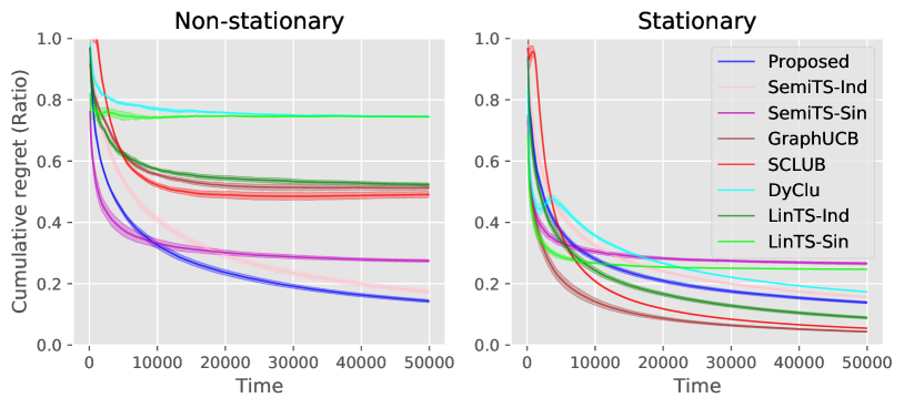
Figure 1: Current cumulative regrets under the non-stationary scenario (left) and the stationary scenario (right). All regrets are relative to that of the random selection.

Figure 1 displays the result for the non-stationary scenario with $\gamma=5$. This scenario satisfies all of our assumptions. As expected, tne proposed SemiGraphTS outperformed other algorithms. Compared to SemiTS-Ind that was the second-best, SemiGraphTS additionally exploited the graph structure, which might have led to the final cumulative regret decreased by 11.5 percent. The third best was SemiTS-Sin, although it performed the best in early rounds. Since SemiTS-Sin estimates only a small number of parameters, the fitted coefficients may have been converging fast to a biased target. Another observation is that SemiGraphTS outperformed the linear graph-based methods. This may suggest that our method could robustly leverage the graph structure when non-stationarity exists. As a next experiment, we tested the same setting but under the stationary scenario $\nu_{j}(t)=0$. Note that both linear and semi-parametric algorithms have theoretical guarantees for this case. The result is reported in the right panel of Figure 1. We see that the linear graph-based algorithms (GraphUCB and SCLUB) outperformed SemiGraphTS. Similarly, LinTS-Ind outperformed SemiTS-Ind. We hypothesize that accommodating the nuisance terms in semi-parametric algorithms may delay convergence of fitted coefficients, which is a price to pay for robustness.

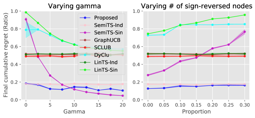
Figure 2: Final cumulative regrets under the non-stationary scenario, while varying $\gamma$ (left) and the proportion of sign-reversed nodes (right). All regrets are relative to that of the random selection.

For sensitivity analysis, we tested the performances of the algorithms against graph strength and graph misspecification. In the left panel of Figure 2, we tracked the final cumulative regrets for varying $\gamma$ from $\gamma=0$ through $\gamma=15$, under the non-stationary scenario. A larger $\gamma$ indicates a stronger similarity between $\mu_{j}$’s. For large-$\gamma$ cases, SemiGraphTS was between those of SemiTS-Ind and SemiTS-Sin. For small-$\gamma$ cases, SemiGraphTS was comparable to SemiTS-Ind and outperformed SemiTS-Sin with a large margin. The right panel of Figure 2 shows the results for misguided graphs, where we varied the proportion of node $j$s in which the signs of $\mu_{j}$ were reversed. When the proportion was large, SemiGraphTS behaved comparably to SemiTS-Ind, while SemiTS-Sin performed poorly.

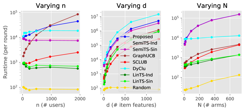
Figure 3: Average runtimes of the algorithms over varying $n$ (left), $d$ (middle), and $N$ (right).

Scalability.

Figure 3 reports the average runtime per step of each algorithm, varying the number of users $n$ (left panel), the number of features $d$ (middle panel), and the number of arms $N$ (right panel), fixing other settings the same as in the non-stationary synthetic experiment. SemiGraphTS was slightly slower than SemiTS-Ind. This difference is expected; the construction of $\widehat{\mu}_{j_{t}}(t)$ and $\Gamma_{j_{t}}(t)$ depends on the degree of the node (user) to serve, which increases linearly with $n$ in the ER graph we tested. A comparison of the semi-parametric methods with the linear methods revealed that each of the semi-parametric methods costed more time than its linear counterparts, mainly due to the Monte Carlo approximation of the arm selection probability. One exception was that SemiGraphTS was faster than GraphUCB as $n$ increases. Overall, SemiGraphTS demonstrated comparable efficiency for large graphs when $d$ and $N$ are in a moderate range.

Real data example.

The LastFM dataset is from a music streaming service last.fm, released by Cantador:RecSys2011. The dataset consists of $n=1,\!892$ nodes (users) connected by $\lvert E\rvert=12,\!717$ edges, and $17,\!632$ items (artists) described by $11,\!946$ tags. It contains an aggregated table for the frequencies of (user, artist) pairs, representing the number of times a user listened to any music of an artist. We generated an artificial history of $t_{0}=5,\!000$ and $T=50,\!000$ rounds following Casa-bianchi2013 and Gentile2014. In short, we randomly sampled one user to serve and $N=25$ artists for each round. As item features, we used the first $d=25$ principal component scores resulting from a term-frequency-inverse-document-frequency (TF-IDF) matrix of artists versus tags, treating artists as “documents” and tags as “words.” We set the reward to 1 if the selected user ever listened to a selected artist and 0 otherwise.

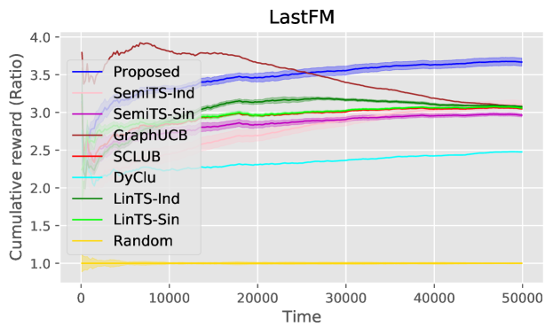
Figure 4: Current cumulative rewards for the LastFM dataset, normalized by the random selection policy.

Figure 4 displays the cumulative rewards of the considered algorithms, relative to that of the random selection policy. SemiGraphTS produced the best final cumulative reward, 16.7 percent higher value compared to the second-best algorithms. In particular, SemiGraphTS uniformly outperformed SemiTS-Ind and SemiTS-Sin, which we believe that the proposed method might have exploited the graph structure successfully. Compared to the linear graph-based algorithms, SemiGraphTS underperformed GraphUCB in early stages but eventually outperformed them. This result is somewhat anticipated from the synthetic experiment; the presence of nuisance term might have slowed down the learning process of the proposed method but enhanced the robustness of against the change of timely trends. To summary the synthetic and real-data experiments, Proposed appears to robustly achieve desirable performances.

6 Concluding Remarks

This study proposes SemiGraphTS, the first algorithm for the semi-parametric contextual bandit MAB problem for multiple users equipped with a graph encoding similarity between user preferences. SemiGraphTS is well suited to more realistic problems in which individual baseline rewards change over time. Experiments demonstrate the potential advantage of SemiGraphTS.

Supplementary Material

In Section A, we introduce lemmas for theoretical derivation. In Appendix B, we complete the proof for Theorem 2. In Appendix C, we provide the proof for Theorem 1. Finally, in Appendix D, we discuss the derivation of the regret bound that addresses the approximation to exact $\pi_{i}(t)$ by Monte Carlo sampling.

Appendix A Auxiliary Lemmas

Lemma 5 (Simplified version of Corollary 4.3 in delaPena2004).

Let $X_{\tau}\in\mathbb{R}^{d}$ and $c_{\tau}\in\mathbb{R}$ be random variables for $\tau=1,\ldots,t$. Let $A(t)\in\mathbb{R}^{d\times d}$ be a symmetric and positive semi-definite matrix. Suppose that, for all $u\in\mathbb{R}^{d}$,

$$\mathbb{E}\left[\exp\left\{u^{T}\sum_{\tau=1}^{t}X_{\tau}c_{\tau}-\frac{1}{2}u^{T}A(t)u\right\}\right]\leq 1.$$

Then, for any $\delta\in(0,1)$ and any symmetric positive definite matrix $Q\in\mathbb{R}^{d\times d}$, the following holds with probability at least $1-\delta$:

$$\left\|\sum_{\tau=1}^{t}X_{\tau}c_{\tau}\right\|_{(Q+A(t))^{-1}}^{2}\leq\log\left\{\frac{\det(Q+A(t))/\det(Q)}{\delta^{2}}\right\}.$$

The lemma below is Lemma 7 in delaPena2009. See also Lemma A.3 of Kim2019 for proof.

Lemma 6.

Let $\{\mathcal{F}_{\tau}\}_{\tau=1}^{t}$ be a filtration. Let $X_{\tau}\in\mathbb{R}^{d}$ and $c_{\tau}\in\mathbb{R}$ be $\mathcal{F}_{\tau}$-measurable random variables such that $\mathbb{E}(X_{\tau}|\mathcal{F}_{\tau-1})=0$, $X_{\tau}\perp c_{\tau}|\mathcal{F}_{\tau-1}$, $\|X_{\tau}\|\leq B$, and $\|c_{\tau}\|\leq 1$ for some constant $B$, $\tau=1,\ldots,t$. Then, for any $u\in\mathbb{R}^{d}$,

$$\mathbb{E}\left[\exp\left\{u^{T}\sum_{\tau=1}^{t}X_{\tau}c_{\tau}-\frac{1}{2}u^{T}\left(\sum_{\tau=1}^{t}X_{\tau}X_{\tau}^{T}+\sum_{\tau=1}^{t}\mathbb{E}(X_{\tau}X_{\tau}^{T}|\mathcal{F}_{\tau-1})\right)u\right\}\right]\leq 1.$$

Lemma 7 (Azuma-Hoeffding inequality).

If $\{M_{t}\}_{t=0}^{T}$ is a supermartingale satisfying $|M_{t}-M_{t-1}|\leq c_{t}$ for all $t$ almost surely, then for any $a>0$,

$$\mathbb{P}\left(|M_{T}-M_{0}|\geq a\right)\leq\exp\left(-\frac{a^{2}}{2\sum_{t=1}^{T}c_{t}^{2}}\right).$$

Lemma 8 (AbramowitzandStegun 1964).

If $Z$ is a standard normal random variable, then for any $u\geq 1$,

$$\frac{1}{2\sqrt{\pi}u}\exp\left(-\frac{u^{2}}{2}\right)\leq\mathbb{P}\left(|Z|>u\right)\leq\frac{1}{\sqrt{\pi}u}\exp\left(-\frac{u^{2}}{2}\right).$$

Appendix B Proof of Theorem 2

The proof of Theorem 2 follows the sketch in the Regret Analysis Section.

B.1 Proof of (11)

By the semi-parametric reward assumption, for $k=1,\ldots,n$,

$$\bar{\mu}_{k}(t) = B_{k}(t)^{-1}\sum_{\tau\in\mathcal{T}_{k,t-1}}2X_{\tau}\left\{\nu(\tau)+b_{\tau}^{T}\mu_{k}+\eta_{\tau}\right\}$$

$$= B_{k}(t)^{-1}\Bigg{\{}\sum_{\tau\in\mathcal{T}_{k,t-1}}2X_{\tau}\nu(\tau)+\sum_{\tau\in\mathcal{T}_{k,t-1}}2X_{\tau}X_{\tau}^{T}\mu_{k}$$

$$~{}~{}~{}~{}+\,\,\sum_{\tau\in\mathcal{T}_{k,t-1}}2X_{\tau}\bar{b}(\tau)^{T}\mu_{k}+\sum_{\tau\in\mathcal{T}_{k,t-1}}2X_{\tau}\eta_{\tau}\Bigg{\}}$$

$$= B_{k}(t)^{-1}\left\{\left(\widehat{\Sigma}_{k,t}+\Sigma_{k,t}\right)+\left(\widehat{\Sigma}_{k,t}-\Sigma_{k,t}\right)+\lambda l_{kk}I_{d}-\lambda l_{kk}I_{d}\right\}\mu_{k}$$

$$~{}~{}~{}~{}+\,\,B_{k}(t)^{-1}\left\{\sum_{\tau\in\mathcal{T}_{k,t-1}}2X_{\tau}\left(\nu(\tau)+\bar{b}(\tau)^{T}\mu_{k}\right)+\sum_{\tau\in\mathcal{T}_{k,t-1}}2X_{\tau}\eta_{\tau}\right\}$$

$$= \mu_{k}-\lambda l_{kk}B_{k}(t)^{-1}\mu_{k}+B_{k}(t)^{-1}A_{k}(t)+B_{k}(t)^{-1}\sum_{\tau\in\mathcal{T}_{k,t-1}}2X_{\tau}\eta_{\tau}.$$

By the relation above, the proposed estimator satisfies

$$\widehat{\mu}_{j}(t)-\mu_{j}$$

$$= -\left[B_{j}(t)^{-1}\sum_{k=1}^{n}\lambda l_{jk}\mu_{k}\right]+\left[B_{j}(t)^{-1}\sum_{k\neq j}\lambda^{2}l_{jk}l_{kk}B_{k}(t)^{-1}\mu_{k}\right]$$

$$~{}~{}~{}+\,2\left[B_{j}(t)^{-1}\sum_{\tau\in\mathcal{T}_{k,t-1}}X_{\tau}\eta_{\tau}\right]-2\left[B_{j}(t)^{-1}\sum_{k\neq j}\lambda l_{jk}B_{k}(t)^{-1}\sum_{\tau\in\mathcal{T}_{k,t-1}}X_{\tau}\eta_{\tau}\right]$$

$$~{}~{}~{}+\,\left[B_{j}(t)^{-1}A_{j}(t)\right]-\left[B_{j}(t)^{-1}\sum_{k\neq j}\lambda l_{jk}B_{k}(t)^{-1}A_{k}(t)\right].$$

Now, left-multiply $b_{i}^{c}(t)^{T}$ on the each side of the equation above and applying Lemma 3 on the six terms in the right-hand side yields the desired result.        $\blacksquare$

B.2 Proof of (15)

Fix $k$ ($k=1,\ldots,n$). Note that when $\mathcal{F}_{\tau-1}$ and $a(\tau)$ are given, $X_{\tau}$ is fixed and $\eta_{\tau}$ is $R$-sub-Gaussian. Then, from (7), for all $u\in\mathbb{R}^{d}$,

$$\mathbb{E}\left[\exp\left\{u^{T}X_{\tau}\left(\frac{\eta_{\tau}}{R}\right)-\frac{1}{2}u^{T}X_{\tau}X_{\tau}^{T}u\right\}\Bigg{|}\mathcal{F}_{\tau-1},a({\tau})\right]\leq 1.$$

This leads to

$$\mathbb{E}\left[\exp\left\{u^{T}\!\!\!\!\sum_{\tau\in\mathcal{T}_{k,t-1}}\!\!\!\!X_{\tau}c_{\tau}-\frac{1}{2}u^{T}\widehat{\Sigma}_{k,t}u\right\}\right]\leq 1,$$

which satisfies the assumption of Lemma 5 with the choice of $X_{\tau}=X_{\tau}$, $c_{\tau}=n_{\tau}/R$, $Q=\lambda l_{kk}I_{d}+\Sigma_{k,t}$ and $A(t)=\widehat{\Sigma}_{k,t}$. Then, for any $0<\delta<1$, with probability at least $1-\delta(\lvert\mathcal{T}_{k,t-1}\rvert+1/n)/(3t^{3})$,

$$\left\|\sum_{\tau\in\mathcal{T}_{k,t-1}}X_{\tau}\eta_{\tau}\right\|_{B_{k}(t)^{-1}}\leq R\sqrt{\log\left\{\frac{\det(B_{k}(t))/\det(\lambda l_{kk}I_{d}+\Sigma_{k,t})}{(\delta(\lvert\mathcal{T}_{k,t-1}\rvert+1/n)/3t^{3})^{2}}\right\}}.$$ (19)

We may assume $\lvert\mathcal{T}_{k,t-1}\rvert\geq 1$, otherwise the left-hand side of (19) is zero. The determinant-trace inequality for $\det(B_{k}(t))$ yields

$$\det(B_{k}(t))\leq\left(\frac{\mathrm{tr}(B_{k}(t))}{d}\right)^{d}$$

$$=\left(\frac{\mathrm{tr}(\lambda l_{kk}I_{d})+\sum_{\tau\in\mathcal{T}_{k,t-1}}\mathrm{tr}(X_{\tau}X_{\tau}^{T}+\mathbb{E}(X_{\tau}X_{\tau}^{T}|\mathcal{F}_{\tau-1}))}{d}\right)^{d}$$

$$\leq\left(\lambda l_{kk}+\frac{8\lvert\mathcal{T}_{k,t-1}\rvert}{d}\right)^{d},$$

where we used $\|X_{\tau}\|\leq 2$. On the other hand, since $\Sigma_{k,t}$ is positive semi-definite, we have $\det(\lambda l_{kk}I_{d}+\Sigma_{k,t})\geq\det(\lambda l_{kk}I_{d})=(\lambda l_{kk})^{d}$. Then, for $d\geq 2$ and $t\geq 1$,

$$\frac{\det(B_{j}(t))}{\det(\lambda l_{kk}I_{d}+\Sigma_{k,t})}\leq\left(1+\frac{8\lvert\mathcal{T}_{k,t-1}\rvert}{d\lambda l_{kk}}\right)^{d}\leq 8^{d}\lvert\mathcal{T}_{k,t-1}\rvert^{d}\left(1+\frac{1}{\lambda l_{kk}}\right)^{d}.$$

Since $d\geq 2$, $t>1$, $0<\delta<1$ and $1\leq\lvert\mathcal{T}_{k,t-1}\rvert\leq t$, the right-hand side of (19) is further simplified by

$$R\sqrt{\log\left\{\frac{\det(B_{k}(t))/\det(\lambda l_{kk}I_{d})}{(\delta(\lvert\mathcal{T}_{k,t-1}\rvert+1/n)/3t^{3})^{2}}\right\}} \leq R\sqrt{\log\left\{\frac{t^{6}}{\delta^{2}}\frac{8^{d}9\lvert\mathcal{T}_{k,t-1}\rvert^{d}\left(1+\frac{1}{\lambda l_{kk}}\right)^{d}}{(\lvert\mathcal{T}_{k,t-1}\rvert+1/n)^{2}}\right\}}$$

$$\leq R\sqrt{\log\left\{\frac{t^{3d}}{\delta^{d}}\frac{8^{d}3^{d}\lvert\mathcal{T}_{k,t-1}\rvert^{d}\left(1+\frac{1}{\lambda l_{kk}}\right)^{d}}{(\lvert\mathcal{T}_{k,t-1}\rvert+1/n)^{2}}\right\}}$$

$$\leq R\sqrt{d\log\left\{\frac{24t^{3}}{\delta}\lvert\mathcal{T}_{k,t-1}\rvert\left(1+\frac{1}{\lambda l_{kk}}\right)\right\}}$$

$$\leq R\sqrt{d\log\left\{\frac{24t^{4}}{\delta}\left(1+\frac{1}{\lambda l_{kk}}\right)\right\}}.$$

Combining (19) and the result above, for any $0<\delta<1$, we have

$$\left\|\sum_{\tau\in\mathcal{T}_{k,t-1}}X_{\tau}\eta_{\tau}\right\|_{B_{k}(t)^{-1}}\leq R\sqrt{d\log\left\{\frac{24t^{4}}{\delta}\left(1+\frac{1}{\lambda l_{kk}}\right)\right\}}$$

with probability at least $\geq 1-\delta(\lvert\mathcal{T}_{k,t-1}\rvert+1/n)/(3t^{3})$. This concludes the derivation.        $\blacksquare$

B.3 Proof of (16)

Fix $k$ ($k=1,\ldots,n$). Recall the definition of $A_{k}(t)$,

$$\left\|A_{k}(t)\right\|_{B_{k}(t)^{-1}}\leq 2\left\|\sum_{\tau\in\mathcal{T}_{k,t-1}}\!\!\!\!X_{\tau}\!\!\left(\nu(\tau)+\bar{b}(\tau)^{T}\mu_{k}\right)\right\|_{B_{k}(t)^{-1}}\!\!\!\!+\left\|\sum_{\tau\in\mathcal{T}_{k,t-1}}\!\!\!\!D_{\tau}\mu_{k}\right\|_{B_{k}(t)^{-1}}\!\!\!\!.$$ (20)

For the first term of the right-hand side of (20), Lemma 6 yields

$$\mathbb{E}\left[\exp\left\{u^{T}\sum_{\tau\in\mathcal{T}_{k,t-1}}X_{\tau}c_{\tau}-\frac{1}{2}u^{T}\left(\widehat{\Sigma}_{k,t}+\Sigma_{k,t}\right)u\right\}\right]\leq 1$$

for any $u\in\mathbb{R}^{d}$, where $c_{\tau}=(\nu(\tau)+\bar{b}(\tau)^{T}\mu_{k})/2$. Then, we can apply Lemma 5 with $A(t)=\widehat{\Sigma}_{k,t}+\Sigma_{k,t}$ and $Q=\lambda l_{kk}I_{d}$ to obtain the following inequality with probability at least $1-\delta(\lvert\mathcal{T}_{k,t-1}\rvert+1/n)/3t^{3}$:

$$\left\|\sum_{\tau\in\mathcal{T}_{k,t-1}}X_{\tau}\left(\nu(\tau)+\bar{b}(\tau)^{T}\mu_{k}\right)\right\|_{B_{k}(t)^{-1}}\leq 2\sqrt{\log\left\{\frac{\det(B_{k}(t))/\det(\lambda l_{kk}I_{d})}{(\delta(\lvert\mathcal{T}_{k,t-1}\rvert+1/n)/3t^{3})^{2}}\right\}}.$$ (21)

We can bound (21) similarly as in bounding the right-hand side of (19). Therefore, with probability at least $1-\delta(\lvert\mathcal{T}_{k,t-1}\rvert+1/n)/3t^{3}$,

$$\left\|\sum_{\tau\in\mathcal{T}_{k,t-1}}X_{\tau}\left(\nu(\tau)+\bar{b}(\tau)^{T}\mu_{k}\right)\right\|_{B_{k}(t)^{-1}}\leq 2\sqrt{d\log\left\{\frac{24t^{4}}{\delta}\left(1+\frac{1}{\lambda l_{kk}}\right)\right\}}.$$ (22)

For the second term of the right-hand side of (20), we let $Y_{k,\tau}=D_{\tau}\mu_{k}$ and observe $Y_{k,\tau}\in\mathbb{R}^{d}$, $\mathbb{E}(Y_{k,\tau}|\mathcal{F}_{\tau-1})=0$. It is straightforward from Lemma 4.4 and its proof in Kim2019 to derive

$$\mathbb{E}\left[\exp\left\{u^{T}\sum_{\tau\in\mathcal{T}_{k,t-1}}\frac{1}{\sqrt{2}}Y_{k,\tau}-\frac{1}{2}u^{T}\left(\widehat{\Sigma}_{k,t}+\Sigma_{k,t}\right)u\right\}\right]\leq 1$$

for any $u\in\mathbb{R}^{d}$, which again satisfies the assumption of Lemma 5 with the choice of $X_{\tau}=Y_{k,\tau}$, $c_{\tau}=1/\sqrt{2}$ and $A(t)=\widehat{\Sigma}_{k,t}+\Sigma_{k,t}$. Then, putting $Q=\lambda l_{kk}I_{d}$, we have with probability at least $1-\delta(\lvert\mathcal{T}_{k,t-1}\rvert+1/n)/3t^{3}$,

$$\left\|\sum_{\tau\in\mathcal{T}_{k,t-1}}D_{\tau}\mu_{k}\right\|_{B_{k}(t)^{-1}} \leq \sqrt{2}\sqrt{\log\left\{\frac{\det(B_{k}(t))/\det(\lambda l_{kk}I_{d})}{(\delta(\lvert\mathcal{T}_{k,t-1}\rvert+1/n)/3t^{3})^{2}}\right\}}$$ (23)

$$\leq \sqrt{2}\sqrt{d\log\left\{\frac{24t^{4}}{\delta}\left(1+\frac{1}{\lambda l_{kk}}\right)\right\}}.$$

Plugging (22) and (23) into (20) yields bounds for each user:

$$\mathbb{P}\left[\left\|A_{k}(t)\right\|_{B_{k}(t)^{-1}}\leq 6\sqrt{d\log\left\{\frac{24t^{4}}{\delta}\left(1+\frac{1}{\lambda l_{kk}}\right)\right\}}\right]\geq 1-\frac{2\delta(\lvert\mathcal{T}_{k,t-1}\rvert+1/n)}{3t^{3}}.$$

Finally, applying the union bound argument yields

$$\mathbb{P}\left[\forall k=1,\ldots,n\,:\,\left\|A_{k}(t)\right\|_{B_{k}(t)^{-1}}\leq 6\sqrt{d\log\left\{\frac{24t^{4}}{\delta}\left(1+\frac{1}{\lambda l_{kk}}\right)\right\}}\right]\geq 1-\frac{2\delta}{3t^{2}},$$ (24)

which completes the proof.        $\blacksquare$

Appendix C Proof of Theorem 1

The proof incorporates the lines of Agrawal2013 and Kim2019 with the proposed estimation and Thompson sampling steps. Throughout the Section, we write as $j=j_{t}$, $b_{\tau}=b_{a(\tau)}(\tau)$ and $\eta_{\tau}=\eta_{a(\tau),j_{\tau}}(\tau)$ for brevity. We reserve $k$ ($k=1,\ldots,k$) to denote user index. The proof has six steps:

• (Theorem 2) To establish a high-probability upper bound of $\lvert b_{i}^{c}(t)(\widehat{\mu}_{j}(t)-\mu_{j})\rvert$.

• (Lemma 9) To establish a high-probability upper bound of $\lvert b_{i}^{c}(t)(\widetilde{\mu}_{j}(t)-\widehat{\mu}_{j}(t))\rvert$ given $\mathcal{F}_{t-1}$.

• (Definition 1) To divide arms at each time $t$ into saturated arms and unsaturated arms.

• (Lemma 10) To bound the probability of playing saturated arms by a function of playing unsaturated arms.

• (Lemma 11) To bound $regret(t)$ given $\mathcal{F}_{t-1}$ for each $t$.

• To bound $R(T)$ and complete the proof.

We begin with step (b).

Lemma 9.

Let $E^{\widetilde{\mu}}(t)$ be an event defined by

$$E^{\widetilde{\mu}}(t)=\left\{\forall i:\lvert b_{i}^{c}(t)^{T}(\widetilde{\mu}_{j}(t)-\widehat{\mu}_{j}(t))\rvert\leq v_{j}s^{c}_{i,j}(t)\min\{\sqrt{4d\log(2dT)},\sqrt{4\log(2NT)}\}\right\}.$$

for all $t\geq 1$, $\mathbb{P}(E^{\widetilde{\mu}}(t)|\mathcal{F}_{t-1})\geq 1-1/T^{2}$.

Proof: We first show $\lvert b_{i}^{c}(t)^{T}(\widetilde{\mu}_{j}(t)-\widehat{\mu}_{j}(t))\rvert\leq v_{j}s^{c}_{i,j}(t)\sqrt{4d\log(2dT)}$. Given $\mathcal{F}_{t-1}$, the values of $b_{i}^{c}(t)$, $\Gamma_{j}(t)$, and $\widehat{\mu}_{j}(t)$ are fixed. Then, for $i=1,\ldots,N$, we have

$$\left|b_{i}^{c}(t)^{T}(\widetilde{\mu}_{j}(t)-\widehat{\mu}_{j}(t))\right| =\left|v_{j}b_{i}^{c}(t)^{T}\Gamma_{j}(t)^{-\frac{1}{2}}\cdot\frac{1}{v_{j}}\Gamma_{j}(t)^{\frac{1}{2}}(\widetilde{\mu}_{j}(t)-\widehat{\mu}_{j}(t))\right|$$

$$\leq v_{j}s^{c}_{i,j}(t)\left\|\frac{1}{v_{j}}\Gamma_{j}(t)^{\frac{1}{2}}(\widetilde{\mu}_{j}(t)-\widehat{\mu}_{j}(t))\right\|_{2}$$

$$=v_{j}s^{c}_{i,j}(t)\sqrt{\sum_{l=1}^{d}Z_{l}(t)^{2}},$$ (25)

where $Z_{l}(t)|\mathcal{F}_{t-1}$ $(l=1,\ldots,d)$ identically and independently follow the standard normal distribution. We apply Lemma 8 with the choice of $u=\sqrt{2\log(2dT^{2})}$. Noting $\sqrt{2\log(2dT^{2})}\leq\sqrt{2\log(2^{2}d^{2}T^{2})}=\sqrt{4\log(2dT)}$,

$$\mathbb{P}\left(\lvert Z_{l}(t)\rvert>\sqrt{4\log(2dT)}\big{|}\mathcal{F}_{t-1}\right)\leq\mathbb{P}\left(\lvert Z_{l}(t)\rvert>\sqrt{2\log(2dT^{2})}\big{|}\mathcal{F}_{t-1}\right)$$

$$\leq\frac{1}{\sqrt{2\pi\log(2dT^{2})}}\cdot\frac{1}{2dT^{2}}\leq\frac{1}{2dT^{2}},$$

for each $l=1,\ldots,d$. Then, by a union bound argument,

$$\mathbb{P}\left(\forall l=1,\ldots,d\,:\,\lvert Z_{k}(t)\rvert>\sqrt{4\log(2dT)}\big{|}\mathcal{F}_{t-1}\right)\leq\frac{1}{2T^{2}}.$$ (26)

Therefore, combining (25) and (26) yields

$$\mathbb{P}\left(\forall i:\left|b_{i}^{c}(t)^{T}(\widetilde{\mu}_{j}(t)-\widehat{\mu}_{j}(t))\right|\leq v_{j}s^{c}_{i,j}(t)\sqrt{4d\log(2dT)}\right)\geq 1-\frac{1}{2T^{2}}.$$

On the other hand, by the observation that $b_{i}^{c}(t)^{T}(\widetilde{\mu}_{j}(t)-\widehat{\mu}_{j}(t))|\mathcal{F}_{t-1}$ $(i=1,\ldots,N)$ identically and independently follow the standard normal distribution, one can apply a similar technique to derive $\lvert b_{i}^{c}(t)^{T}(\widetilde{\mu}_{j}(t)-\widehat{\mu}_{j}(t))\rvert\leq v_{j}s^{c}_{i,j}(t)\sqrt{4\log(2NT)}$ with probability at least $1-1/(2T^{2})$ given $\mathcal{F}_{t-1}$. Combining the two bounds, we obtain the desired result.

In step (c), we divide arms at each time $t$ into saturated arms and unsaturated arms. Note that $C(t)$ implitly depends on $j_{t}$.

Definition 1.

Define $C(t)$, the set of saturated arms, by

$$C(t)=\{i:b_{i}^{c}(t)^{T}\mu_{j}+g_{j}(T)s^{c}_{i,j}(t)<b_{a^{*}(t)}(t)^{T}\mu_{j}\},$$

where $g_{k}(T)=\alpha_{k}(T)+v_{k}\min\{\sqrt{4d\log(2dT)},\sqrt{4\log(2NT)}\}$ and $\alpha_{k}(T)=(4R+12)\cdot$ $\sqrt{d\log\left\{(24T^{4}/\delta)(1+\lambda^{-1})\right\}}+\sqrt{\lambda}(1+\|\Delta_{k}\|)$, $k=1,\ldots,n$.

In step (d), we establish that the probability of playing saturated arms is bounded by the probability of playing unsaturated arms up to constant multiplication and addition.

Lemma 10.

Given $\mathcal{F}_{t-1}$ such that $E^{\widehat{\mu}}(t)$ is true,

$$\mathbb{P}\left(a(t)\in C(t)|\mathcal{F}_{t-1}\right)\leq\frac{1}{p}\mathbb{P}\left(a(t)\notin C(t)|\mathcal{F}_{t-1}\right)+\frac{1}{pT^{2}},$$

where $p=1/(4e\sqrt{\pi})$.

Proof: Since $a(t)=\operatornamewithlimits{argmax}_{1\leq i\leq N}\{b_{i}^{c}(t)^{T}\widetilde{\mu}_{j}(t)\}$ by definition, if $b_{a^{*}(t)}(t)^{T}\widetilde{\mu}_{j}(t)>b_{i}^{c}(t)^{T}\widetilde{\mu}_{j}(t)$ for every $i\in C(t)$, then $a(t)\notin C(t)$. This implies

$$\mathbb{P}\left(a(t)\notin C(t)|\mathcal{F}_{t-1}\right)\geq\mathbb{P}\left(\forall i\in C(t):b_{a^{*}(t)}(t)^{T}\widetilde{\mu}_{j}(t)>b_{i}^{c}(t)^{T}\widetilde{\mu}_{j}(t)|\mathcal{F}_{t-1}\right).$$ (27)

On the other hand, when $E^{\widetilde{\mu}}(t)$ is additionally true,

$$b_{i}^{c}(t)^{T}\widetilde{\mu}_{j}(t) \leq b_{i}^{c}(t)^{T}\mu_{j}+g_{j}(T)s^{c}_{i,j}(t) E^{\widehat{\mu}}(t) E^{\widetilde{\mu}}(t)$$ (Def. of & )

$$\leq b_{a^{*}(t)}(t)^{T}\mu_{j}, \mbox{(Def. of $C(t)$)},$$

which implies that

$$\mathbb{P}\left(b_{a^{*}(t)}(t)^{T}\mu_{j}<b_{a^{*}(t)}(t)^{T}\widetilde{\mu}_{j}(t)|\mathcal{F}_{t-1}\right)$$

$$\leq\mathbb{P}\left(\forall i\in C(t):b_{i}^{c}(t)^{T}\widetilde{\mu}_{j}(t)<b_{a^{*}(t)}(t)^{T}\widetilde{\mu}_{j}(t)|\mathcal{F}_{t-1}\right)+\left(1-\mathbb{P}\left(E^{\widetilde{\mu}}(t)|\mathcal{F}_{t-1}\right)\right)$$ (28)

The left-hand side of (28) can be lower-bounded, because the normality of $\widetilde{\mu}_{j}(t)$ and Lemma 8 yields

$$\mathbb{P}\left(b_{a^{*}(t)}(t)^{T}\widetilde{\mu}_{j}(t)>b_{a^{*}(t)}(t)^{T}\mu_{j}\Big{|}\mathcal{F}_{t-1}\right)$$

$$=\mathbb{P}\left(\frac{b_{a^{*}(t)}(t)^{T}(\widetilde{\mu}_{j}(t)-\widehat{\mu}_{j}(t))}{v_{j}s^{c}_{a^{*}(t),j}(t)}>\frac{b_{a^{*}(t)}(t)^{T}(\mu_{j}-\widehat{\mu}_{j}(t))}{v_{j}s^{c}_{a^{*}(t),j}(t)}\Big{|}\mathcal{F}_{t-1}\right)$$

$$\geq\mathbb{P}\left(Z(t)>\frac{\alpha_{j}(T)}{v_{j}}\big{|}\mathcal{F}_{t-1}\right)$$

$$\geq\frac{1}{4\sqrt{\pi}u}\exp\left(-\frac{u^{2}}{2}\right),$$

where $u=\alpha_{j}(T)/v_{j}$ and $Z(t)|\mathcal{F}_{t-1}$ is a standard normal random variable. Note that $u\leq 1$ by the construction. Therefore,

$$\mathbb{P}\left(b_{a^{*}(t)}(t)^{T}\widetilde{\mu}_{j}(t)>b_{a^{*}(t)}(t)^{T}\mu_{j}|\mathcal{F}_{t-1}\right)\geq\frac{1}{4e\sqrt{\pi}}=p.$$ (29)

Combining (27), (28), (29) and Lemma 9, we have

$$\mathbb{P}\left(a(t)\notin C(t)|\mathcal{F}_{t-1}\right)+\frac{1}{T^{2}}\geq p,$$

which implies

$$\frac{\mathbb{P}\left(a(t)\in C(t)|\mathcal{F}_{t-1}\right)}{\mathbb{P}\left(a(t)\notin C(t)|\mathcal{F}_{t-1}\right)+\frac{1}{T^{2}}}\leq\frac{1}{p}.$$

This completes the proof.

Before proceeding to bound the cumulative regret, we bound each $regret(t)$ given $\mathcal{F}_{t-1}$ in step (e).

Lemma 11.

Given $\mathcal{F}_{t-1}$ such that $E^{\widehat{\mu}}(t)$ is true,

$$\mathbb{E}\left(regret(t)|\mathcal{F}_{t-1}\right)\leq\frac{5g_{j}(T)}{p}\mathbb{E}\left(s^{c}_{a(t),j}(t)|\mathcal{F}_{t-1}\right)+\frac{4g_{j}(T)}{pT^{2}}.$$

Proof: Let $\bar{a}(t)=\operatornamewithlimits{argmin}_{i\notin C(t)}s^{c}_{i,j}(t)$. If $\mathcal{F}_{t-1}$ is given, then $\bar{a}(t)$ is deterministic. This value is also well-defined due to $a^{*}(t)\notin C(t)$. Under $\mathcal{F}_{t-1}$ such that both $E^{\widehat{\mu}}(t)$ and $E^{\widetilde{\mu}}(t)$ holds,

$$b_{a^{*}(t)}(t)^{T}\mu_{j}$$

$$=b_{a^{*}(t)}(t)^{T}\mu_{j}-b_{\bar{a}(t)}(t)^{T}\mu_{j}+b_{\bar{a}(t)}(t)^{T}\mu_{j}$$

$$\leq g_{j}(T)s^{c}_{\bar{a}(t),j}(t)+b_{\bar{a}(t)}(t)^{T}\mu_{j} \bar{a}(t)\notin C(t) C(t)$$ ( & def. of )

$$\leq g_{j}(T)s^{c}_{\bar{a}(t),j}(t)+b_{\bar{a}(t)}(t)^{T}\widetilde{\mu}_{j}(t)+g_{j}(T)s^{c}_{\bar{a}(t),j}(t) E^{\widehat{\mu}}(t) E^{\widetilde{\mu}}(t)$$ (Def. of and )

$$\leq 2g_{j}(T)s^{c}_{\bar{a}(t),j}(t)+b_{a(t)}(t)^{T}\widetilde{\mu}_{j}(t) a(t)$$ (Def. of )

$$\leq 2g_{j}(T)s^{c}_{\bar{a}(t),j}(t)+b_{a(t)}(t)^{T}\mu_{j}+g_{j}(T)s^{c}_{a(t),j}(t) \mbox{(Def. of $E^{\widehat{\mu}}(t)$ and $E^{\widetilde{\mu}}(t)$)},$$

which yields

$$regret(t)\leq 2g_{j}(T)s^{c}_{\bar{a}(t),j}(t)+g_{j}(T)s^{c}_{a(t),j}(t).$$

Then, under $\mathcal{F}_{t-1}$ such that $E^{\widehat{\mu}}(t)$ holds, the following holds from inequality above, Lemma 9 and $\lvert regret(t)\rvert\leq 2$:

$$\mathbb{E}\left(regret(t)|\mathcal{F}_{t-1}\right)$$ (30)

$$= \mathbb{E}\left(regret(t)I(E^{\widetilde{\mu}}(t))|\mathcal{F}_{t-1}\right)+\mathbb{E}\left(regret(t)\{1-I(E^{\widetilde{\mu}}(t))\}|\mathcal{F}_{t-1}\right)$$

$$\leq 2g_{j}(T)s^{c}_{\bar{a}(t),j}(t)+g_{j}(T)\mathbb{E}\left(s^{c}_{a(t),j}(t)|\mathcal{F}_{t-1}\right)+2\left(1-\mathbb{P}\left(E^{\widetilde{\mu}}(t)|\mathcal{F}_{t-1}\right)\right)$$

$$\leq 2g_{j}(T)s^{c}_{\bar{a}(t),j}(t)+g_{j}(T)\mathbb{E}\left(s^{c}_{a(t),j}(t)|\mathcal{F}_{t-1}\right)+\frac{2}{T^{2}}.$$

We now further bound $s^{c}_{\bar{a}(t),j}(t)$. Observe that

$$s^{c}_{\bar{a}(t),j}(t)$$

$$=s^{c}_{\bar{a}(t),j}(t)\left\{\mathbb{P}(a(t)\in C(t)|\mathcal{F}_{t-1})+\mathbb{P}(a(t)\notin C(t)|\mathcal{F}_{t-1})\right\}$$

$$=s^{c}_{\bar{a}(t),j}(t)\left\{\frac{2}{p}\mathbb{P}(a(t)\notin C(t)|\mathcal{F}_{t-1})+\frac{1}{pT^{2}}\right\}$$ (Lemma 10)

$$=\frac{2}{p}\mathbb{E}\left(s^{c}_{\bar{a}(t),j}(t)I(a(t)\notin C(t))|\mathcal{F}_{t-1}\right)+\frac{s^{c}_{\bar{a}(t),j}(t)}{pT^{2}}$$

$$\leq\frac{2}{p}\mathbb{E}\left(s^{c}_{a(t),j}(t)I(a(t)\notin C(t))|\mathcal{F}_{t-1}\right)+\frac{s^{c}_{\bar{a}(t),j}(t)}{pT^{2}} \bar{a}(t)$$ (Def. of )

$$\leq\frac{2}{p}\mathbb{E}\left(s^{c}_{a(t),j}(t)|\mathcal{F}_{t-1}\right)+\frac{1}{pT^{2}}. s^{c}_{i,k}(t)\leq 1 i,k,t$$ ( for any )

Combining the inequality above and (30) conclude the proof.

In step (f), we complete the proof.

Proof: [Proof for Theorem 1] Let

$$M_{t}:=regret(t)I(E^{\widehat{\mu}}(t))-\frac{5g_{j_{t}}(T)}{p}s_{a(t),j_{t}}(t)-\frac{4g_{j_{t}}(T)}{pT^{2}},~{}t=1,\ldots,T,$$

with $M_{0}=0$.

We apply martingale arguments for each user $k=1,\ldots,n$, and aggregate them by union bound. Fix $k$ and let $T_{k}=\lvert\mathcal{T}_{k,T}\rvert$. Due to Lemma 11 and $s^{c}_{i,k}(t)\leq 1$, $\{M_{t}\}_{t\in\{0\}\cup\mathcal{T}_{k,T}}$ is a supermartingale process satisfying $\lvert M_{t}\rvert\leq 10g_{k}(T)/p$. We apply Lemma 7 with the choice of $c_{t}=10g_{k}(T)/p$ and $a=(10g_{k}(T)/p)\sqrt{2T_{k}\log(2T/(\delta T_{k}))}$ that satisfies $\exp(-a^{2}/(2\sum_{t}c_{t}^{2}))=\delta T_{k}/(2T)$. This yields

$$\sum_{t\in\mathcal{T}_{k,T}}regret(t)I(E^{\widehat{\mu}}(t))\leq$$

$$\frac{5g_{k}(T)}{p}\sum_{t\in\mathcal{T}_{k,T}}s^{c}_{a(t),k}(t)+\frac{4g_{k}(T)}{pT}+\frac{10g_{k}(T)}{p}\sqrt{2T_{k}\log(2T/(\delta T_{k}))}$$ (31)

with probability at least $1-\delta T_{k}/(2T)$. Since $T_{1}+\ldots+T_{n}=T$, a union bound argument over $k=1,\ldots,n$ leads to

$$\sum_{t=1}^{T}regret(t)I(E^{\widehat{\mu}}(t))\leq$$

$$\sum_{k=1}^{n}\left[\frac{5g_{k}(T)}{p}\sum_{t\in\mathcal{T}_{k,T}}s_{a(t),k}(t)+\frac{4g_{k}(T)}{pT}+\frac{10g_{k}(T)}{p}\sqrt{2T_{k}\log(2T/(\delta T_{k}))}\right]$$ (32)

with probability at least $1-\delta/2$.

On the other hand, we apply a union bound argument to Theorem 2 over $t=1,\ldots,T$ and replace $\delta$ with $3\delta/\pi^{2}$, which yields $\mathbb{P}(E^{\widehat{\mu}}(t)\mbox{ for all $t=1,\ldots,T$})\geq 1-\delta/2$. Then, $regret(t)I(E^{\widehat{\mu}}(t))=regret(t)$ for every $t$ with probability at least $1-\delta/2$.

Therefore, with probability at least $1-\delta$,

$$\sum_{t=1}^{T}regret(t)\leq\sum_{k=1}^{n}\left[\frac{5g_{k}(T)}{p}\!\!\sum_{t\in\mathcal{T}_{k,T}}\!\!s^{c}_{a(t),k}(t)+\frac{4g_{k}(T)}{pT}+\frac{10g_{k}(T)}{p}\sqrt{2T_{k}\log(2T/(\delta T_{k}))}\right].$$

Now, by Lemma 12 below and the definitions of $g_{k}(T)$ and $p$,

$$R(T)\leq\sum_{k=1}^{n}O\Bigg{(}\!\Psi_{k,T}\left\{\!\sqrt{d\log(\lvert\mathcal{T}_{k,T}\rvert)}\!+\!\sqrt{\lambda}\|\Delta_{k}\|\!\right\}\!\times$$

$$\min\!\left\{\!\sqrt{d\log(d\lvert\mathcal{T}_{k,T}\rvert)},\!\sqrt{\log(N\lvert\mathcal{T}_{k,T}\rvert)}\!\right\}\!\sqrt{d\lvert\mathcal{T}_{k,T}\rvert\log(\lvert\mathcal{T}_{k,T}\rvert)}\Bigg{)}$$

with probability at least $1-\delta$, which completes the proof.

Lemma 12.

$$\sum_{t\in\mathcal{T}_{k,T}}s^{c}_{a(t),k}(t)=O\left(\Psi_{k,T}\sqrt{d\lvert\mathcal{T}_{k,T}\rvert\log(\lvert\mathcal{T}_{k,T}\rvert)}\right).$$

Proof: We recall that $\Psi_{k,T}=\sum_{t\in\mathcal{T}_{k,T}}\|X_{t}\|_{\Gamma_{k}(t)^{-1}}/\sum_{t\in\mathcal{T}_{k,T}}\|X_{t}\|_{B_{k}(t)^{-1}}$ and that $\Psi_{k,T}\in(0,1)$ due to $\Gamma_{k}(t)^{-1}<B_{k}(t)^{-1}$ for all $j$, $t$. Since $\sum_{t\in\mathcal{T}_{k,T}}s^{c}_{a(t),k}(t)=\sum_{t\in\mathcal{T}_{k,T}}\|X_{t}\|_{\Gamma_{k}(t)^{-1}}$ by the definitions of $s^{c}_{i,k}(t)$ and $X_{t}$, we have

$$\sum_{t\in\mathcal{T}_{k,T}}s^{c}_{a(t),k}(t)=\Psi_{k,T}\sum_{t\in\mathcal{T}_{k,T}}\|X_{\tau}\|_{B_{k}(t)^{-1}}.$$

We now claim $\sum_{t\in\mathcal{T}_{k,T}}\|X_{\tau}\|_{B_{k}(t)^{-1}}=O\left(\sqrt{d\lvert\mathcal{T}_{k,T}\rvert\log(\lvert\mathcal{T}_{k,T}\rvert)}\right)$. This has been proved in similar settings (Abbasi-Yadko, 2011; Agrawal2013; Vaswani2017; Kim2019); for completeness, we present the proof. Define $s_{i,k}(t)=\|b_{i}^{c}(t)\|_{B_{j}(k)^{-1}}$. Note that $s_{a(t),j_{t}}(t)=X_{t}$ and $\sum_{t\in\mathcal{T}_{k,T}}\|X_{\tau}\|_{B_{k}(t)^{-1}}=$. Then, $\|X_{\tau}\|_{B_{k}(t)^{-1}}=\sum_{t\in\mathcal{T}_{k,T}}s_{a(t),k}(t)$. Following the lines for equation 60 of Vaswani2017, we can derive

$$\log\left[\det(B_{k}(t+1))\right]\geq\log\left[\det(\lambda l_{kk}I_{d})\right]+\sum_{\tau\in\mathcal{T}_{k,t}}\log\left(1+s_{a(\tau),k}(\tau)^{2}\right).$$ (33)

On the other hand, the trace of $B_{k}(t+1)$ is

$$\mathrm{tr}\left(B_{k}(t+1)\right)\leq 8\lvert\mathcal{T}_{k,T}\rvert+\lambda l_{kk}d,$$ (34)

where we used $\|X_{\tau}\|\leq 2$ by construction. Plugging (33) and (34) into the determinant-trace inequality $\left\{\mathrm{tr}\left(B_{k}(t+1)\right)/d\right\}^{d}\geq\det\left(B_{k}(t+1)\right)$, equivalently $d\log\left\{\mathrm{tr}\left(B_{k}(t+1)\right)/d\right\}\geq\log\det\left(B_{k}(t+1)\right)$, we obtain

$$d\log\left(\frac{8\lvert\mathcal{T}_{k,T}\rvert}{d}+\lambda l_{kk}\right)\geq d\log(\lambda l_{kk})+\sum_{\tau\in\mathcal{T}_{k,t}}\log\left(1+s_{a(\tau),k}(\tau)^{2}\right),$$

or,

$$\sum_{\tau\in\mathcal{T}_{k,t}}\log\left(1+s_{a(\tau),k}(\tau)^{2}\right)\leq d\log\left(1+\frac{8\lvert\mathcal{T}_{k,T}\rvert}{d\lambda l_{kk}}\right).$$

Now, we bound $\sum_{\tau\in\mathcal{T}_{k,t}}s_{a(\tau),k}(\tau)^{2}$ by the result above. First, we have $s_{a(\tau),k}(\tau)^{2}\in[0,1/(\lambda l_{kk})]$ because

$$s_{a(\tau),k}(\tau)^{2}=b_{\tau}^{T}B_{k}(\tau)^{-1}b_{\tau}\leq b_{\tau}^{T}\left(\lambda l_{kk}I_{d}\right)^{-1}b_{\tau}\leq(\lambda l_{kk})^{-1}.$$

Considering a function $f(t)=\log(1+t)/\left[\lambda l_{kk}\log\left(1+(\lambda l_{kk})^{-1}\right)\right]$, $f$ satistfies $t\leq f(t)$ for all $t\in[0,1/(\lambda l_{kk})]$. Therefore,

$$\sum_{\tau\in\mathcal{T}_{k,t}}s_{a(\tau),k}(\tau)^{2} \leq \frac{1}{\lambda l_{kk}\log\left(1+(\lambda l_{kk})^{-1}\right)}\sum_{\tau\in\mathcal{T}_{k,t}}\log\left(1+s_{a(\tau),k}(\tau)^{2}\right)$$

$$\leq \frac{d}{\lambda l_{kk}\log\left(1+(\lambda l_{kk})^{-1}\right)}\log\left(1+\frac{\lvert\mathcal{T}_{k,T}\rvert}{d\lambda l_{kk}}\right).$$

Finally, from the Cauchy-Schwartz inequality and the result above,

$$\sum_{\tau\in\mathcal{T}_{k,t}}s_{a(\tau),k}(\tau) \leq \sqrt{8\lvert\mathcal{T}_{k,T}\rvert}\sqrt{\sum_{\tau\in\mathcal{T}_{k,t}}s_{a(\tau),k}(\tau)^{2}}$$

$$\leq \sqrt{\frac{d\lvert\mathcal{T}_{k,T}\rvert}{\lambda l_{kk}\log\left(1+(\lambda l_{kk})^{-1}\right)}\log\left(1+\frac{\lvert\mathcal{T}_{jk,t}\rvert}{d\lambda l_{kk}}\right)}.$$

Since $l_{kk}=1$ by the defintion of the random-walk Laplacian,

$$\sum_{\tau\in\mathcal{T}_{k,t}}s_{a(\tau),k}(\tau)\leq\sqrt{\frac{d\lvert\mathcal{T}_{k,T}\rvert}{\lambda\log\left(1+\frac{1}{\lambda}\right)}\log\left(1+\frac{8\lvert\mathcal{T}_{k,T}\rvert}{d\lambda}\right)},$$

which proves the claim and concludes the proof.

Appendix D Regret bound when $\pi_{i}(t)$ is approximated by Monte Carlo sampling

In this section, we analyze the additional regret induced by approximation and show that the regret upper bound of the alternative algorithm has the same order as the bound of SemiGraphTS.

Our discussion is based on Algorithm 2, a special case of the SemiGraphTS algorithm (Algorithm 1), that explicitly states that we use the Monte Carlo approximated values of $\pi_{i}(t)$ for action selection. Before action selection, Algorithm 2 computes first the Monte Carlo approximates of $\pi_{i}(t)$. We denote the approximated value as $\widehat{\pi}_{i}(t).$ Then, Algorithm 2 samples the arm from a multinomial distribution with size 1, say ${\rm Multinom}(\widehat{\pi}_{1}(t),\cdots,\widehat{\pi}_{N}(t))$. In comparison, Algorithm 1 samples $a(t)\sim{\rm Multinom}(\pi_{1}(t),\cdots,\pi_{N}(t))$.

Algorithm 2 A special case of the SemiGraphTS algorithm that approximates $\pi_{i}(t)$ by the Monte Carlo sampling (SemiGraphTS-MC)

1:Fix $\lambda>0$ and M. Set $B_{j}(1)=\lambda l_{jj}I_{d}$, $y_{j}(1)=0_{d}$ and $v_{j}=(4R+12)\sqrt{d\log\left\{({24}T^{4}/\delta)(1+\lambda^{-1})\right\}}+\sqrt{\lambda}(1+\|\Delta_{j}\|)$ for $j=1,\ldots,n$.

2:for $t=1,2,\ldots,T$ do

3:     Observe $j_{t}$.

4:     for $j=1,2,\ldots,n$ do

5:         if $j\neq j_{t}$ then

6:              Update $B_{j}(t+1)\leftarrow B_{j}(t)$, $\bar{\mu}_{j}(t+1)\leftarrow\bar{\mu}_{j}(t)$, and $y_{j}(t+1)\leftarrow y_{j}(t)$.

7:         else

8:              $\widehat{\mu}_{j}(t)\leftarrow\bar{\mu}_{j}(t)-B_{j}(t)^{-1}\sum_{k\neq j}\lambda l_{jk}\bar{\mu}_{k}(t)$.

9:              $\Gamma_{j}(t)\leftarrow B_{j}(t)+\lambda^{2}\!\sum_{k\neq j}\!l_{jk}^{2}\!B_{k}(t)^{-1}$

10:              for $m=1,2,\cdots,M$ do

11:                  Sample $\widetilde{\mu}_{j}^{m}(t)$ from $\mathcal{N}_{d}(\widehat{\mu}_{j}(t),v_{j}^{2}\Gamma_{j}(t)^{-1})$

12:              end for

13:              for $i=1,2,\cdots,N$ do

14:                  Compute $\widehat{\pi}_{i}(t)=\frac{1}{M}\sum_{m=1}^{M}I\left\{i=\operatornamewithlimits{argmax}_{k}\{b_{k}(t)^{T}\widetilde{\mu}_{j}^{m}(t)\}\right\}$

15:              end for

16:              Sample $a(t)$ from ${\rm Multinom}(\widehat{\pi}_{1}(t),\cdots,\widehat{\pi}_{N}(t))$.

17:              $\bar{b}(t)\!\leftarrow\!\sum_{i=1}^{N}\!\widehat{\pi}_{i}(t)b_{i}(t)$ and $X_{t}\!\leftarrow\!b_{a(t)}(t)-\bar{b}(t)$.

18:              Update $B_{j}(t+1)\!\leftarrow\!B_{j}(t)\!+\!X_{t}X_{t}^{T}\!+\!\sum_{i=1}^{N}\!\widehat{\pi}_{i}(t)(b_{i}(t)-\bar{b}(t))(b_{i}(t)-\bar{b}(t))^{T}$, $y_{j}(t+1)\!\leftarrow\!y_{j}(t)\!+\!2X_{t}r_{a(t),j}(t)$, and $\bar{\mu}_{j}(t+1)\!\leftarrow\!B_{j}(t+1)^{-1}y_{j}(t+1)$.

19:         end if

20:     end for

21:end for

We now discuss the regret bound for Algorithm 2. We highlight the key differences from following the lines of Section C. Let the filtration $\mathcal{F}_{t-1}$ further include all Monte Carlo samples up to time $t-1$.

For step (a), Theorem 2 directly holds with $\pi_{i}(t)$’s replaced with $\widehat{\pi}_{i}(t)$’s since the approximated values $\widehat{\pi}_{i}(t)$’s are now the true probabilities of the arm selection.

Steps (b)-(e) in Section C exploited that the arm is selected form the exact probability. In other words, those results were derived if we select arm according to $\tilde{a}(t)=\operatornamewithlimits{argmax}_{1\leq i\leq N}\{b_{i}(t)^{T}\widetilde{\mu}_{j_{t}}(t)\}$ (i.e., $\widetilde{a}(t)\sim{\rm Multinom}(\pi_{1}(t),\cdots,\pi_{N}(t))$). Now we show through an inductive argument that the remaining proofs are still valid with the new arm selection $a(t)\sim{\rm Multinom}(\widehat{\pi}_{1}(t),\cdots,\widehat{\pi}_{N}(t))$.

Suppose that until round $t-1$, we have sampled arms $a(\tau)\sim{\rm Multinom}(\widehat{\pi}_{1}(\tau),\cdots,\widehat{\pi}_{N}(\tau))$, $\tau=1,\cdots,t-1$. Then we have the desired high-probability upper bound for the estimate $\hat{\mu}_{j}(t)$ for every $j=1,\cdots,n$ (Theorem 2). Now suppose that at round $t$, we sample the arm $\tilde{a}(t)=\operatornamewithlimits{argmax}_{1\leq i\leq N}\{b_{i}(t)^{T}\widetilde{\mu}_{j_{t}}(t)\}$. Then the proofs (b)-(e) go through, and by Lemma 13 we have,

$$\mathbb{E}\left((b_{a^{*}(t)}(t)^{T}\mu_{j_{t}}-b_{\tilde{a}(t)}(t)^{T}\mu_{j_{t}})I(E^{\hat{\mu}}(t))|\mathcal{F}_{t-1}\right)$$

$$\leq\frac{5g_{j_{t}}(T)}{p}\mathbb{E}\left(s^{c}_{{\tilde{a}}(t),{j_{t}}}(t)|\mathcal{F}_{t-1}\right)+\frac{4g_{j_{t}}(T)}{pT^{2}}.$$ (35)

Then, given $\mathcal{F}_{t-1}$ such that $E^{\hat{\mu}}(t)$ is true,

$$\mathbb{E}\left(regret(t)|\mathcal{F}_{t-1}\right)$$

$$=\mathbb{E}\left(b_{a^{*}(t)}(t)^{T}\mu_{j_{t}}-b_{{a}(t)}(t)^{T}\mu_{j_{t}}|\mathcal{F}_{t-1}\right)$$

$$=\mathbb{E}\left((b_{a^{*}(t)}(t)^{T}\mu_{j_{t}}-b_{\tilde{a}(t)}(t)^{T}\mu_{j_{t}})+(b_{\tilde{a}(t)}(t)^{T}\mu_{j_{t}}-b_{{a}(t)}(t)^{T}\mu_{j_{t}})|\mathcal{F}_{t-1}\right)$$

$$\leq\frac{5g_{j_{t}}(T)}{p}\mathbb{E}\left(s^{c}_{{\tilde{a}}(t),{j_{t}}}(t)|\mathcal{F}_{t-1}\right)+\frac{4g_{j_{t}}(T)}{pT^{2}}+\mathbb{E}\left(b_{\tilde{a}(t)}(t)^{T}\mu_{j_{t}}-b_{{a}(t)}(t)^{T}\mu_{j_{t}}|\mathcal{F}_{t-1}\right)$$

$$=\frac{5g_{j_{t}}(T)}{p}\mathbb{E}\left(s^{c}_{{{a}}(t),{j_{t}}}(t)|\mathcal{F}_{t-1}\right)+\frac{4g_{j_{t}}(T)}{pT^{2}}+\mathbb{E}\left(b_{\tilde{a}(t)}(t)^{T}\mu_{j_{t}}-b_{{a}(t)}(t)^{T}\mu_{j_{t}}|\mathcal{F}_{t-1}\right)$$

$$~{}~{}~{}~{}+\frac{5g_{j_{t}}(T)}{p}\mathbb{E}\left(s^{c}_{{{\tilde{a}}}(t),{j_{t}}}(t)-s^{c}_{{{a}}(t),{j_{t}}}(t)|\mathcal{F}_{t-1}\right).$$

As compared to Lemma 13 for Algorithm 1, we have two additional terms to bound; for step (f), those terms appear in the final cumulative regret. We claim below that the cumulative sum of the two additional terms have lower order than the original regret bound of Algorithm 1. We first have,

$$\mathbb{E}\left(b_{\tilde{a}(t)}(t)^{T}\mu_{j_{t}}-b_{{a}(t)}(t)^{T}\mu_{j_{t}}|\mathcal{F}_{t-1}\right)$$

$$=\mathbb{E}\left(\sum_{i=1}^{N}b_{i}(t)^{T}\mu_{j_{t}}I(\tilde{a}(t)=i)-\sum_{i=1}^{N}b_{i}(t)^{T}\mu_{j_{t}}I(a(t)=i)\Big{|}\mathcal{F}_{t-1}\right)$$

$$=\sum_{i=1}^{N}b_{i}(t)^{T}\mu_{j_{t}}\pi_{i}(t)-\sum_{i=1}^{N}b_{i}(t)^{T}\mu_{j_{t}}\mathbb{E}(\widehat{\pi}_{i}(t)|\mathcal{F}_{t-1})$$

$$=\sum_{i=1}^{N}b_{i}(t)^{T}\mu_{j_{t}}\pi_{i}(t)-\sum_{i=1}^{N}b_{i}(t)^{T}\mu_{j_{t}}\pi_{i}(t)=0,$$

which is due to unbiasedness of the Monte-Carlo estimate $\widehat{\pi}_{i}(t)$. Since we also have $\text{b\_}\tilde{\text{a}}\text{(t)(t)^T}\text{μ}\text{\_j\_t-b\_a(t)(t)^T}\text{μ}\text{\_j\_t}\text{ ≤2},wecanshowfromtheAzuma-Hoeffidinginequality,withhighprobability,\text{(36)Equation 3636∑t=1T{b~a(t)(t)Tμjt-ba(t)(t)Tμjt}≤O(T).}Similarly,wehave\begin{array}{cc}& {\displaystyle \frac{5g{}_{j{}_t}(T)}{p}}𝔼(s{}^c{}_{\tilde{a}(t),j{}_t}(t)-s{}^c{}_{a(t),j{}_t}(t)|ℱ{}_{t-1})\hfill \\ & ={\displaystyle \frac{5g{}_{j{}_t}(T)}{p}}𝔼({\displaystyle \sum }{}_{i=1}{}^{N}s{}^c{}_{i,j{}_t}(t)I(\tilde{a}(t)=i)-{\displaystyle \sum }{}_{i=1}{}^{N}s{}^c{}_{i,j{}_t}(t)I(a(t)=i)|ℱ{}_{t-1})\hfill \\ & ={\displaystyle \frac{5g{}_{j{}_t}(T)}{p}}{\displaystyle \sum }{}_{i=1}{}^{N}s{}^c{}_{i,j{}_t}(t)(\pi {}_i(t)-\pi {}_i(t))=0.\hfill \end{array}Hencewithhighprobability,\text{(37)Equation 3737∑t=1T5gjt(T)p{sc~a(t),jt(t)-sca(t),jt(t)}≤5maxjgj(T)pO(T).}Weremarkthattheright-handsidesof(\text{<a href="\#A4.E36" title="In Appendix D Regret bound when 𝜋\_{𝑖}(𝑡) is approximated by Monte Carlo sampling ‣ Semi-Parametric Contextual Bandits with Graph-Laplacian Regularization" class="ltx\_ref ltx\_font\_italic"><span class="ltx\_text ltx\_ref\_tag">36</span></a>})and(\text{<a href="\#A4.E37" title="In Appendix D Regret bound when 𝜋\_{𝑖}(𝑡) is approximated by Monte Carlo sampling ‣ Semi-Parametric Contextual Bandits with Graph-Laplacian Regularization" class="ltx\_ref ltx\_font\_italic"><span class="ltx\_text ltx\_ref\_tag">37</span></a>})doesnotdependon\text{d, n, N}northegraphstructure.Therefore,ourclaimholds.\text{References11964AbramowitzandStegunAbramowitzandStegun(1964)Abramowitz1964}Abramowitz,M.;andStegun,I.1964.\text{Handbook of Mathematical Functions with Formulas, Graphs, and Mathematical Tables}.UnitedStatesDepartmentofCommerce,NationalBureauofStandards.\text{22011Abbasi-Yadko}$