Bankrupting DoS Attackers

Abstract

Abstract. To defend against denial-of-service (DoS) attacks, we employ a technique called resource burning (RB). RB is the verifiable expenditure of a resource, such as computational power, required from clients before receiving service from the server. To the best of our knowledge, we present the first DoS defense algorithms where the algorithmic cost — the cost to both the server and the honest clients — is bounded as a function of the attacker’s cost.

We model an omniscient, Byzantine attacker, and a server with access to an estimator that estimates the number of jobs from honest clients in any time interval. We examine two communication models: an idealized zero-latency model and a partially synchronous model. Notably, our algorithms for both models have asymptotically lower costs than the attacker’s, as the attacker’s costs grow large. Both algorithms use a simple rule to set required RB fees per job. We assume no prior knowledge of the number of jobs, the adversary’s costs, or even the estimator’s accuracy. However, these quantities parameterize the algorithms’ costs.

We also prove a lower bound on the cost of any randomized algorithm. This lower bound shows that our algorithms achieve asymptotically tight costs as the number of jobs grows unbounded, whenever the estimator output is accurate to within a constant factor.

1 Introduction

Money is the key to understanding modern denial-of-service (DoS) attacks. On one side, attackers spend money to rent botnets to submit spurious jobs. On the other side, service providers spend money to provision additional cloud resources to prevent service disruptions [81]. Thus, DoS attacks have shifted from traditional resource bottlenecks—such as computational power—to monetary cost. Additionally, motivation for attack has shifted towards extortion; an easily achievable goal whenever the cost to attack is less than the cost to defend.

These new DoS attacks are commonly referred to as economic denial-of-sustainability (EDoS) [68, 45, 20, 69]. A major challenge for defenders is setting the correct amount of provisioning, in order to manage costs, while continuing to provide service [81, 82, 86]. The problem has significant economic motivation since the average cost of a DoS attack can be in the millions of dollars [47].

It has long been suggested that a fee for service could be used to moderate DoS attacks [27, 41, 6, 74, 54, 76, 62]. Here, we design strategies for setting this fee in an online manner, by a server who is assisted by an estimate of the number of jobs from honest clients which have recently been submitted. Our goal is to require an aggressive adversary to pay asymptotically more than the amount paid by both the honest clients and the server. To the best of our knowledge, we give the first DoS defense algorithms with formal guarantees on the defense cost as a function of the attack cost.

1.1 Our Problem

Resource Burning. Resource burning (RB) is the verifiable expenditure of a network resource, such as computational power, computer memory, or bandwidth [4, 37, 39, 40]. For a specific value $h$, we define a $\mathbf{h}$-hard RB challenge as a RB task requiring expenditure of $h$ units of the resource; an RB threshold is the required value $h$. The solution to an $h$-hard RB challenge is an $\mathbf{h}$-hard RB solution. We do not address the problem of designing RB challenges in this paper; however, significant prior work addresses this, with possible resources such as computational power [76], bandwidth [75], computer memory [1], or human effort [72, 63].

Server and Clients. In our problem, there is a server and clients. The server receives a stream of jobs. Each job is either good: sent by a client; or bad: sent by the adversary (described below).

There are no simultaneous events: job generation and message receipt occur one at a time in a stream. Additionally, clients and the adversary can directly send messages to the server, and the server can directly send a message to any client. The following happens in parallel for the server and clients.

• Server: The server uses the estimator to compute the current RB threshold. Jobs received by the server are serviced based on whether the RB solution attached meets the required RB threshold. When the server receives a job request that it does not service, it sends the current RB threshold back to the client or the adversarial identity that made the request.

• Clients: Each client may send a job to the server with an RB solution attached of any hardness.

Thus, there are two types of messages sent: (1) RB threshold changes, sent from the server to the clients; and (2) jobs with attached RB solutions, sent from clients to the server.

Byzantine Adversary. A Byzantine adversary seeks to maximize the cost of our algorithm. This adversary knows our algorithm before execution begins, and it adaptively sets the distribution of good and bad jobs.

Costs. Our algorithmic costs are two-fold. The first is RB costs incurred by clients. The second is provisioning costs incurred by the server: the cost required to service a job (good or bad), which we assume is a normalized value of $1$.

The cost to the adversary equals the total cost of all RB challenges that it solves.

The Estimator. The server has access to an estimator that it may use to set the RB threshold. An estimator estimates the number of good jobs generated in any contiguous time interval seen so far. For any such interval, $\mathcal{I}$, let $g(\mathcal{I})$ be the number of good jobs in $\mathcal{I}$ and $\hat{g}(\mathcal{I})$ be the value returned by the estimator for interval $\mathcal{I}$. The estimator $\hat{g}$ is additive: for any two non-overlapping intervals, $\mathcal{I}_{1}$ and $\mathcal{I}_{2}$:

$$\hat{g}(\mathcal{I}_{1}\cup\mathcal{I}_{2})=\hat{g}(\mathcal{I}_{1})+\hat{g}(\mathcal{I}_{2}).$$

For a given input, the estimation gap, $\gamma$, is the smallest positive integer such that the following holds for all intervals, $\mathcal{I}$ in the input:

$$g(\mathcal{I})/\gamma-\gamma\leq\hat{g}(\mathcal{I})\leq\gamma g(\mathcal{I})+\gamma$$

Our model does not assume a specific estimator implementation. But in Section 4.1, we provide an example estimator with small $\gamma$ value, given plausible assumptions about the input.

Communication Latency. We consider two problem variants:

• Without Latency: All messages are sent instantaneously. So, the clients always know the exact threshold value; and the RB solutions attached to jobs sent to the server always arrive before any change in threshold value, and thus are always serviced.

• With Latency: Communication is partially synchronous [26, 52]: there is some maximum latency, $L$ seconds, for any message to be received after it is sent. Also, there is some maximum number of good jobs, $M$, that can be generated over $L$ seconds. Both $L$ and $M$ are unknown to the algorithm, but known to the adversary. Also, the adversary controls the timing of messages subject to the above constraints.

(Lack of) Knowledge of the Servers and Clients. Other than what is given by the estimator, the server and clients have no prior knowledge of the number of good jobs, the amount spent by the Byzantine adversary, or the estimation gap. Recall that, in the latency model, $L$ and $M$ are also unknown.

1.2 Our Results

For a given input, let $g$ be the number of good jobs, $B$ be the total cost to the Byzantine adversary, and $\gamma$ be the estimation gap for the input. Our primary goal is to minimize the algorithmic cost — i.e. RB costs for good jobs plus provisioning costs for the server — as a function of $g$, $B$, and $\gamma$

We first describe and analyze an algorithm LINEAR for the without-latency problem variant. Our first result is the following (See Sections 3.1 and 5).

Theorem 1.1.

LINEAR has total cost

$$O(\gamma^{5/2}\sqrt{B\,(g+1)}+\gamma^{3}(g+1)).$$

Moreover, the server sends $O(g)$ messages to clients, and clients send a total of $O(g)$ messages to the server. Also, each good job is serviced after an exchange of at most $3$ messages.

To build intuition for this result, consider the case where $\gamma=O(1)$. Then, the theorem states that the cost to LINEAR is $O(\sqrt{B(g+1)}+(g+1))$. Importantly, the cost to the algorithm grows asymptotically slower than $B$ whenever $g=o(B)$. We note that the additive $O(g+1)$ term results from provisioning costs due to good jobs, which must hold for any algorithm.

Finally, the number of messages sent from server to clients and from clients to server, and also the maximum number of messages exchanged to obtain service are all asymptotically optimal. To see this note that at least one message must be sent for each good job serviced.

What if there is latency? For our with-latency variant, we design and analyze an algorithm LINEAR-POWER. Our main theorem for this case is as follows; the $\tilde{O}$ notation for the algorithmic cost hides terms that are logarithmic in $B$ and $\gamma$ (see Lemma 12 for precise asymptotics).

Theorem 1.2.

LINEAR-POWER has total cost:

$$\tilde{O}\left(\gamma^{3}\left(\sqrt{B+1}\min\left(g+1,M\sqrt{g+1},M\sqrt{B+1}\right)+(g+1)\right)\right).$$

Moreover, the server sends $O(g\log(B+2\gamma^{2}))$ messages to clients, and clients sends a total of $O(g\log(B+2\gamma^{2}))$ messages to the server. Also, each good job is serviced after an exchange of at most $4\log(\gamma(B+1))+3$ messages.

To gain intuition for this result, assume that $\gamma$ and $M$ are both $O(1)$. Then the cost to LINEAR-POWER is $\tilde{O}\left(\sqrt{B+1}\min\left(\sqrt{g+1},\sqrt{B+1}\right)+(g+1)\right)$. This equals $\tilde{O}(\sqrt{B(g+1)}+(g+1))$, since when $B=O(g)$, the expression is $\tilde{O}(g+1)$; and otherwise the expression is $\tilde{O}(\sqrt{B(g+1)})$. Thus, when $\gamma$ and $M$ are constants, the cost of LINEAR-POWER matches that of LINEAR, up to logarithmic terms. For communication, the number of messages sent from the server to clients, clients to the server, and the maximum number of message exchanges before job service all increase by a logarithmic factor in $B$, when compared to LINEAR.

To complement these upper bounds, in Section 7, we also prove the following lower bound. This lower bound holds for our without-latency variant, and so directly also holds for the harder, with-latency variant.

Theorem 1.3.

Let $\gamma$ be any positive integer; $g_{0}$ be any positive multiple of $\gamma$; and $n$ any multiple of $\gamma g_{0}$. Next, fix any randomized algorithm. Then, there is an input with $n$ jobs, $g$ of which are good for $g\in\{\gamma g_{0},g_{0}/\gamma\}$; and an estimator with gap $\gamma$ on that input. Additionally, the randomized algorithm on that input has expected cost:

$$E(A)=\Omega\left(E(\sqrt{\gamma B(g+1)})+\gamma(g+1)\right).$$

When $\gamma=O(1)$, this lower bound asymptotically matches the cost for LINEAR, and is within logarithmic factors of the cost for LINEAR-POWER. Additionally, the lower bound allows for a fair amount of independence between the settings of $\gamma$, $g$ and $n$ for which the lower bound can be proven. For example, it holds both when $g$ is small compared to $n$ and also when $g$ is large. Finally, note that the lower bound holds for randomized algorithms, even though both LINEAR and LINEAR-POWER are deterministic. Thus, randomization does not offer significant improvements for our problem.

Finally, we simulate LINEAR in the without-latency variant, and LINEAR-POWER in the with-latency variant, in Section 8. In these simulations, we compare the algorithm’s cost to the adversary’s cost when all good jobs are serviced as late as possible. Our results suggest that the hidden constants in the asymptotic notation may be small, and that the scaling behavior for our algorithms’ costs matches what is predicted by theory.

1.3 Technical Overview

In this section, we give intuition for all of our technical results.

Without Latency. Our algorithm for the without-latency problem is LINEAR. Here, we give a high-level overview of the algorithm and its analysis, see Section 3.1 for detailed pseudocode and Section 5 for a formal analysis.

LINEAR is conceptually simple. Time is partitioned into iterations, which end whenever the estimator returns a value of at least $1$ for the estimate of the number of good jobs seen in the iteration so far. The RB threshold is set to $s$, where $s$ is the number of jobs seen so far in the iteration.

To analyze the cost for LINEAR, we first show: (1) upper and lower bounds on the number of iterations in LINEAR as a function of $\gamma$, $g$ and $n$ (Lemmas 1 and 3); and (2) an upper bound on the number of good jobs in any iteration (Lemma 2).

Next, using (1) and (2), we prove an upper bound on the cost of LINEAR. To be systematic, we consider a class of threshold setting algorithms where the charge to the $s$-th job in the iteration is $s^{\alpha}$, for any constant $\alpha\geq 0$, and we prove that $\alpha=1$ gives the best algorithmic cost as a function of $B$, $g$ and $\gamma$.

Our upper bound consists of four exchange arguments - the first two lower bound $B$ and the next two upper bound $A$. We begin by lower bounding $B$. To do so, our first exchange argument shows that $B$ is minimized when, in each iteration, the bad jobs occur before the good. Our second exchange argument shows that, subject to this constraint, $B$ is minimized when the bad jobs are distributed as evenly as possible across the iterations. From these two exchange arguments, a lower bound on $B$ follows via an integral lower bound and basic algebra (see Lemma 4).

We next upper bound $A$. To do so, we first make two observations: (1) within an iteration, $A$ is maximized by putting all good jobs at the end; and (2) without loss of generality, we can assume that the iterations are sorted in decreasing order by the number of bad jobs they contain. Then we use the third (simple) exchange argument to show that $A$ is maximized when good jobs are “packed left”: packed as much as possible in the earlier iterations, which have the higher number of bad jobs.

Finally, we use the fourth (harder) exchange argument to show that $A$ is maximized when bad jobs are “packed left” when $\alpha\geq 1$, and are evenly spread when $\alpha<1$. To show this, for an iteration $i$, we let $f(b_{i})$ be the cost of the $i$-th iteration when there are $b_{i}$ bad jobs at the start. Then, let $\Delta(b_{i})=f(b_{i}+1)-f(b_{i})$ be the change in the cost of iteration $i$ when we add $1$ bad job. Then the change in cost when there is an exchange of one bad job from iteration $k$ to iteration $i$ for $k>i$ will be $\Delta(b_{i})-\Delta(b_{k}-1)$.

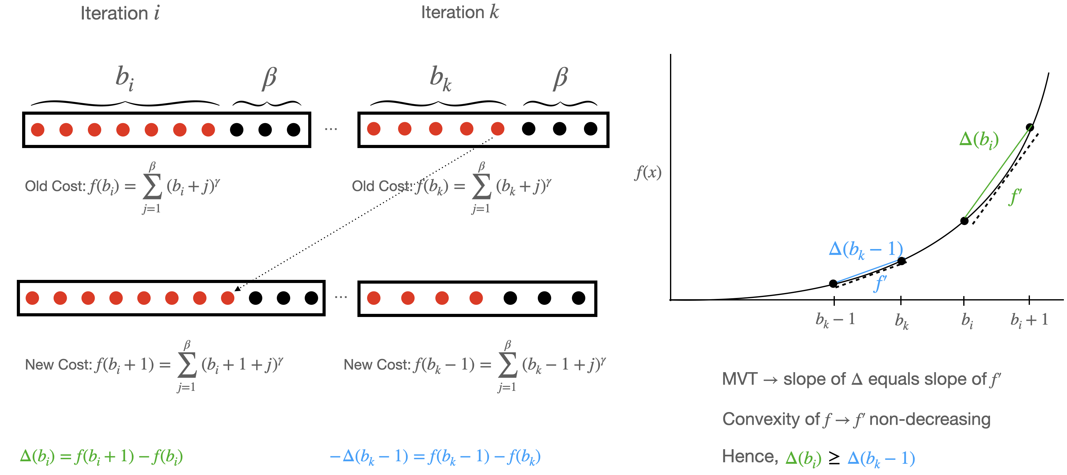
Figure 5: Illustration of an exchange of one bad job (a red ball) from iteration $k$ to iteration $i$, with all good jobs (black balls) remaining in place. The change in cost for iteration $i$ is $\Delta(b_{i})$, and change in cost for iteration $k$ is $\Delta(b_{k}-1)$. The Mean Value Theorem (MVT) says that for any integer $x$, the value of $\Delta(x)$ equals $f^{\prime}(y)$ for some $y\in[x,x+1]$. Using the convexity of $f^{\prime}$ (for $\alpha\geq 1$), this implies that $\Delta(b_{i})\geq\Delta(b_{k}-1)$. This means that the exchange shown can only increase the algorithmic cost.

How do we show that $\Delta(b_{i})-\Delta(b_{k}-1))\geq 0$? If we relax $b_{i}$ so it can take on values in the real numbers, then $f(b_{i})$ becomes a continuous, differentiable function. Thus, we can use the mean value theorem (MVT). In particular, the MVT shows that $\Delta(b_{i})$ equals $f^{\prime}(x)$ at some value of $x\in[b_{i},b_{i+1}]$. Then, upper and lower bounding the $\Delta$ values reduces to bounding $f^{\prime}$ in the appropriate range. This is a simpler problem because $f^{\prime}$ is a monotonically non-decreasing (non-increasing) function when $\alpha\geq 1$ ($\alpha<1$, respectively). Once we have this exchange argument in hand, calculating the algorithmic costs is fairly straightforward; see Lemma 5, Figure 5, and Theorem 1.1 for details.

With Latency. If we naively use LINEAR for the with-latency model, the total cost can be high. To get a simple analysis, assume that $\gamma=\Theta(1)$ and $g=\Theta(M\sqrt{B})$. Then, the adversary can insert $\sqrt{B}$ bad jobs initially, causing the threshold value in LINEAR to increase $\sqrt{B}$ times. During this time $\Theta\left(\min\left(g,M\sqrt{B}\right)\right)$ good jobs join the system, all of them bouncing repeatedly as the threshold value increases, until the threshold reaches its maximum value of $\Theta(\sqrt{B})$. Next, all $\Theta\left(\min(g,M\sqrt{B})\right)$ of these good jobs wind up paying an RB cost equal to $\Theta(\sqrt{B})$. Adding in the cost to service jobs and the cost for any additional good jobs that enter after the bad, we have a total cost for the LINEAR of $\Theta\left(\min\left(g+1,M\sqrt{B+1}\right)\sqrt{B+1}+g\right)$.

How can we improve this? One key idea is to reduce the number of times that the server increases the threshold. Our second algorithm, LINEAR-POWER does just that: (1) the server sets the threshold value to the largest power of $2$ less than the total number of jobs in the current iteration; and (2) clients double their RB value whenever their job bounces.

To compare LINEAR-POWER with LINEAR, suppose $\gamma=O(1)$. Then, it is not hard to see that in any iteration $i$ where the adversary spends $B_{i}$, the maximum threshold value is $O(\sqrt{B_{i}})$ (see Lemma 8). Thus, we can argue that any job is bounced $O(\log B)$ times, and pays a total of $O(\sqrt{B})$.

But the above argument gives a poor bound on RB costs for the clients, since it multiplies all such costs from the LINEAR analysis by a $\sqrt{B}$ factor. To do better, we need a tighter analysis for RB costs. But how do we precede when a single job can be refused service over many iterations because it keeps learning the threshold value too late?

The first key idea is to partition time into epochs. An epoch is a period of time ending with $2L$ seconds during which the server threshold value never increases. Then, several facts follow. First, every good job is serviced within $2$ epochs. Second, we can bound the total cost that all good jobs pay during epoch $i$ to be essentially $O(M(\sqrt{B_{i-1}}+\sqrt{B_{i}}))$, where $B_{j}$ is the amount spent by the adversary in epoch $j$ (see Lemma 11). Third, an epoch has overpaying jobs only if it or its preceding epoch spans the beginning of an iteration (see Lemma 10). This last fact allows us to bound the total number of epochs that add to the overpayment amount using our previous bounds on the number of iterations. Putting all these facts together, we obtain a cost for LINEAR-POWER that is only $\tilde{O}\left(\min\left(g+1,M\sqrt{g+1},M\sqrt{B+1}\right)\sqrt{B+1}+g\right)$ (see Theorem 1.2) versus the cost of LINEAR computed above of $\Theta\left(\min\left(g+1,M\sqrt{B+1}\right)\sqrt{B+1}+g\right)$. Ignoring logarithmic factors, the cost of LINEAR-POWER may be less than LINEAR by a factor of $\sqrt{g+1}/M$. As an example, when $M=O(1)$ and $B=\Theta(g)$, LINEAR-POWER has cost $\tilde{O}(g)$, and LINEAR has cost $\Theta(g^{3/2})$.

Lower Bound Without Latency. In Section 7, we prove a lower bound for our problem variant without latency. This bound directly holds for our harder, with-latency problem variant.

In our lower bound, for given values of $\gamma$, $g_{0}$ and $n$, we design an input distribution that (1) sets $g$ to $g_{0}/\gamma$ with probability $1/2$, and sets $g$ to $\gamma g_{0}$ otherwise; (2) distributes $g$ good jobs uniformly but randomly throughout the input; and (3) creates an estimator that effectively hides both the value of $g$ and also the location of the good jobs, and always has estimation gap at most $\gamma$ on the input (See Section 7.1 and Lemma 16 for details).

The key technical challenge is to set up a matrix in order to use Yao’s minimax principle [79] to prove a lower bound on the expected cost for any randomized algorithm. In particular, we need a game-theory payoff matrix where the rows are deterministic algorithms, and the columns are deterministic inputs. A natural approach is for the matrix entries to be the ratios $A/\sqrt{Bg}$. Unfortunately, this fails to achieve our goal since this would yield $E[A/\sqrt{Bg}]$ and we need $E[A]/E[\sqrt{Bg}]$, which are not generally equal. Some lower bound proofs can circumvent this type of problem. For example, lower bound proofs on competitive ratios of online algorithms circumvent the problem because the offline cost does not vary with the choice of the deterministic algorithm, i.e. from row to row. So the expected offline cost can be factored out and computed separately (see [14], Chapter 5). Unfortunately, this does not work for us since our random variables $A$ and $B$ are interdependent, and vary across both rows and columns.

We solve this problem by first setting the matrix entries to $E(A)-\sqrt{E(B)g\gamma})$, and then proving that the minimax for such a payoff matrix has expected value at least $0$. Then, we use Jensen’s inequality and linearity of expectation to show that the minimax is also at least $0$ when the matrix entries are $E(A-\sqrt{Bg\gamma})$ (see Lemma 17). Next, using Yao’s principle, we can show the maximin is nonnegative, and thereby obtain a key inequality for $A$ and $B$. Once we have this inequality, we can use algebra to establish our lower bound for any randomized algorithm (see Theorem 1.3).

We believe that this new approach – using Yao’s principle on a matrix whose entries are $X-Y$ in order to bound the ratio $E(X)/E(Y)$, and thereby prove some target lower bound of $E(Y)$ – may have broader applications to proving lower bounds for resource competitive algorithms [10, 32].

1.4 A Roadmap

The remainder of our paper is organized as follows. In Section 2, we discuss closely-related work and how it connects with our results. Our algorithms, LINEAR and LINEAR-POWER, are described in Section 3. In Section 4, we give an example estimator, and we discuss some example scenarios for both algorithms. Our upper-bound proofs are presented in Sections 5 and 6, while our lower-bound argument is given in Section 7. In Section 8, we report our simulation results. We conclude and discuss some future research directions in Section 9.

2 Related Work

2.1 DoS Attacks and Defenses

DoS attacks are a persistent threat, with current trends pointing to an increase in their occurrence [46]; consequently, the associated literature is vast. Here, we discuss prior results most pertinent to our approach.

Resource Burning for DoS. Many DoS defenses use resource-burning, requiring clients to solve computational challenges. Early work by Juels and Brainard [41] examines cryptographic puzzles to mitigate connection depletion attacks, such as TCP SYN flooding. Work by Aura et al. [6] followed soon after, looking to apply computational puzzles to more general DoS attacks. In contrast to computational resources, Walfish et al. [74] propose a defense that instead burns communication capacity.

Some defenses rely on the participation of routers. For example, Parno et al. [64] look at how capabilities (informally, where routers prioritize specific traffic flows to the server) can be defended against DoS attacks via computational puzzles. Work by Chen et al. [19] also makes use of routers to filter traffic flows, but with a focus on minimizing modifications to the network architecture.

Methods have been explored for appropriately tuning the hardness of RB challenges. Mankins et al. [54] explore methods of pricing access to the server resources based on client behavior, where the costs imposed can be either monetary or computational. Along similar lines, Wang and Reiter [76] explore ways that clients can bid on puzzles via auctions. More recently, Noureddine et al. [62] apply game theory to determine the difficulty of the computational challenges used in the context of DoS attacks at the transport layer.

Other works have focused on specific practical aspects related to DoS defense. User experience is addressed by Kaiser and Feng [42], who provide a browser plugin that makes a computational puzzle-based DoS defense largely transparent to the user. Another issue is the wasted work inherent in solving puzzles, and Abliz and Znati [2] propose the use of puzzles whose solutions provide useful work on real applications/services.

Generally, all of the above-mentioned approaches have clients quickly increase the amount of RB until service is received. However, these approaches do not account for on-demand provisioning, nor do they provide an asymptotic advantage to the defense algorithm over the adversary in terms of total algorithmic cost, where the algorithmic cost equals the client RB costs plus the server provisioning costs.

Finally, we note that all prior RB-based defenses [64, 62, 42, 74, 76, 6] fail against a sufficiently powerful adversary. This is also true of more traditional defenses, such as those based on over-provisioning and replication. This is unsurprising, since DDoS attacks are notoriously challenging and no single technique offers a full solution. In our approach, we have tried to (1) incorporate costs incurred to the algorithm for dropping jobs, servicing jobs, and solving challenges; and (2) minimize these costs as a function of the adversary’s costs, when the adversarial costs are unbounded.

Generating Challenges and Verifying Solutions. Challenge generation and validation are efficient operations, and in our model they have zero cost. However, this functionality is itself subject to attack [5] and must itself be protected. Fortunately, unlike the range of services offered by the server, the narrow functionality of generating and validating challenges can be easily outsourced and scaled, while being resistant to attack (see [77]). In practice, a dedicated service can provide this narrow functionality, and jobs may contact this service to receive a challenge and have their solutions verified.

Provisioning Costs. Many servers are equipped with sufficient resources to handle good jobs. However, during a DoS attack, additional resources must be provisioned on-demand. This imposes an economic cost on the system that grows as a function of the traffic load. In practice, the cost for DoS protection can be significant and is a factor in how defenses are designed [82, 86, 8].

2.2 Resource Burning

Starting with the seminal 1992 paper by Dwork and Naor [27], there has been significant academic research, spanning multiple decades, on using RB to address many security problems; see surveys [4, 37]. Security algorithms that use resource burning arise in the domains of wireless networks [35], peer-to-peer systems [50, 13], blockchains [51], and e-commerce [37]. Our algorithm is purposefully agnostic about the specific resource burned, which can include computational power [76], bandwidth [75], computer memory [1], or human effort [72, 63]. Unfortunately, despite this prior work, there are few RB results in the literature that bound the defender’s cost as a function of the attacker’s.

2.3 Algorithms with Predictions

Algorithms with predictions is a new research area which seeks to use predictions to achieve better algorithmic performance. In general, the goal is to design an algorithm that performs well when prediction accuracy is high, and where performance drops off gently with decreased prediction accuracy. Critically, the algorithm has no a priori knowledge of the accuracy of the predictor on the input.

The use of predictions offers a promising approach for improving algorithmic performance. This approach has found success in the context of contention resolution [33]; bloom filters [56]; online problems such as job scheduling [65, 49, 67]; and many others. See surveys by Mitzenmacher and Vassilvitskii [58, 59]. Our estimation gap for the input, $\gamma$ is related to a accuracy metric for a predictor of job lengths in [67].

Critically, our estimator differs from predictions in that it never returns results predicting the future, it only estimates the number of good jobs in past intervals.

Classification and Filtering. Differentiating good and bad jobs can be challenging, since clients often enjoy a large degree of anonymity, and face little-to-no admission control for using a service. Nonetheless, classifiers are a common method for mitigating DoS attacks. A classification accuracy above 95% has been demonstrated [24, 60, 83]. However, with classification alone, the server can still incur significant provisioning costs since some constant fraction of the bad jobs may bypass the classifier. Thus, classification is not a silver bullet, but rather part of a more comprehensive defense.

Many DoS defenses rely on a range of techniques for filtering out malicious traffic [85], including IP profiling [53, 80]; and capability-based schemes [5, 78]. These techniques are complimentary to our proposed approach and can further reduce the volume of malicious traffic. However, again, they are not a solution by themselves, as they may err. Even if the error rate is a small constant, classification and filtering alone can not ensure that algorithmic provisioning cost will be asymptotically smaller than the attacker’s cost. That said, machine learning techniques for classification [17, 66, 71] may help improve the accuracy of an estimator on inputs that are likely to occur in practice.

2.4 Resource-Competitive Algorithms

There is a growing body of research on security algorithms whose costs are parameterized by the adversary’s cost. Such results are often referred to as resource-competitive [11]. Specific recent results in this area include algorithms to address: malicious interference on a broadcast channel [34, 31, 44, 18], contention resolution [9], interactive communication [23, 3], the Sybil attack [38, 36], and bridge assignment in Tor [84]. To the best of our knowledge, our result is the first that uses an estimator, and incorporates the estimation gap on the input into the algorithmic cost.

2.5 Game theory

Many research results analyze security problems in a game theoretic setting. These include two-player security games between an attacker and defender, generally motivated by the desire to protect infrastructure (airports, seaports, flights, networks) [70, 7, 73] or natural resources (wildlife, crops) [29, 28]. Recently, Kempe, Schulman and Tamuz [43] define a quite general game based on choices the defender and attacker make about how much time they spend visiting a set of targets. Their game abstracts many of the above applications, and they formally show how one can compute optimal defender play for the game via quasi-regular sequences.

Additionally, game theoretic security problems may include multiple players, and have a mix of Byzantine, altruistic and rational (BAR) players. See [22, 21] for an overview of BAR games.

Finally, resource burning is analogous to what is called money burning or costly signaling [12, 40] in the game theory literature. See Hartline and Roughgarden [39] for applications of this to algorithmic game theory via auction design.

In our paper, we do not assume the adversary, server or clients are rational. Our main results show how to minimize the server and clients costs as a function of the adversarial cost. This is different than optimizing most typical utility functions for the defender. However, there are two game theoretic connections. First, when there exists an algorithm for the defender, as in this paper, where the defender pays some function $f$ of the adversarial cost $B$, and $f(B)=f(0)+o(B)$, it is possible to solve a natural zero-sum, two-player attacker-defender game. The solution of this game is for the attacker to set $B=0$ — essentially to not attack — in which case the defender pays a cost of $f(0)$, which in our case is $O(\gamma^{3}g)$ (See Section 2.6 of [37] for details). Second, our paper suggests, for future work, the game-theoretic problem of refining our current model and algorithms in order to build a mechanism for clients and a server that are all selfish-but-rational (Section 9).

3 Our Algorithms

In Section 3.1, we formally define the algorithm LINEAR; and in Section 3.2, we define the algorithm LINEAR-POWER. As described in Section 1.1, both of our algorithms make use of an estimator. So in Section 4.1, we give an example of the type of estimator that might be used by these algorithms. Next, in Section 4.2, to build intuition, we will give some example scenarios for our algorithms.

3.1 Algorithm LINEAR

Our first algorithm, LINEAR, addresses our without-latency problem variant. The server partitions the servicing of jobs into iterations, which end when $\hat{g}(\mathcal{I})\geq 1$, where $\mathcal{I}$ is the time interval in the current iteration. The threshold value, THRESH, for the next job is set to $s+1$, where $s$ is the number of jobs serviced so far in the iteration. Since there is no latency, good jobs will always send in RB solutions with value equal to THRESH, thus jobs with lower value solutions can be ignored. Pseudocode is given in Figure 1. Again, because there is no latency, the client’s action is just to either send in the job with attached RB solution equal to the current value of THRESH, or else drop the job.

Figure 1: Pseudocode for LINEAR.

3.2 Algorithm LINEAR-POWER

We next describe a second algorithm, LINEAR-POWER, that addresses the with-latency variant of our problem; see Figure 2 for the pseudocode.

Server. The server operates in iterations, which end when $\hat{g}(\mathcal{I})\geq 1$, where $\mathcal{I}$ is the time interval elapsed in the iteration. During an iteration, the server repeatedly processes the next job.

The threshold value, THRESH, is set to $2^{\lfloor\log(s+1)\rfloor}$, where $s$ is the number of jobs serviced so far in the iteration. If the RB value attached to the next job is at least THRESH, the job is serviced. Otherwise, the job is not serviced, and the server sends a message with the value THRESH to the client that sent the job.

Client. To begin, a client sends the server a $1$-hard RB solution with its job. Initially, let $x\leftarrow 1$. When the client receives a message from the server with a THRESH value greater than $x$, it (1) sets $x$ to be the threshold value received; and (2) sends the server a $x$-hard RB solution with its job, or chooses to drop the job.

Figure 2: Pseudocode for LINEAR-POWER.

4 Example Estimator and Scenarios

In this section, we give an example estimator and scenario examples for both LINEAR and LINEAR-POWER.

4.1 Example Estimator

Recall that our problem model (Section 1.1) is purposefully agnostic to the type of estimator used. However, we now describe one possible estimator.

Consider an input where good jobs are generated via a Poisson distribution with parameter $\lambda$, so that the expected interval length between good jobs is $1/\lambda$. Let $P=\{k/\lambda:k\in\mathbb{Z}^{+}\}$, i.e. P is the set of all points in time which are positive multiples of $1/\lambda$. Then, for any interval $\mathcal{I}$, let:

$$\hat{g}(\mathcal{I})=|\mathcal{I}\cap P|$$

To evaluate this estimator, consider any input distribution with $g$ good jobs generated by this Poisson process. We show that with high probability, i.e. probability at least $1-1/g^{k}$ for any positive $k$, $\hat{g}$ enures $\gamma=O(\log g)$.

To show this, for an interval $\mathcal{I}$, let $\ell(\mathcal{I})$ be the length of $\mathcal{I}$, and recall that $g(\mathcal{I})$ is the number of good jobs generated during $\mathcal{I}$. We rely on the following fact which holds by properties of the Poisson process, Chernoff and union bounds.

Fact 1.

The following holds, w.h.p., for any interval $\mathcal{I}$, and for some constant $C$:

1. If $g(\mathcal{I})<C\ln g$, then $\ell(\mathcal{I})=O((1/\lambda)\log g)$

2. If $g(\mathcal{I})\geq C\ln g$, then $\ell(\mathcal{I})=\Theta((1/\lambda)g(\mathcal{I}))$.

Now, consider two cases:

Case: $g(\mathcal{I})<C\ln g$. Then, by Fact 1 (1), $\ell(\mathcal{I})=O((1/\lambda)\log g)$, and so $\hat{g}(\mathcal{I})=O(\log g)$. Thus, there exists some $\gamma$, $\gamma=O(\log g)$ such that

$$g(\mathcal{I})-\gamma\leq\hat{g}(\mathcal{I})\leq g(\mathcal{I})+\gamma$$

Hence, the estimation gap on this type of interval is $O(\log g)$.

Case: $g(\mathcal{I})\geq C\ln g$. Then by Fact 1 (2), w.h.p., $\ell(\mathcal{I})=\Theta((1/\lambda)g(\mathcal{I}))$, and so $\hat{g}(\mathcal{I})=\Theta(g(\mathcal{I}))$. So, there exists some $\gamma$, $\gamma=O(1)$ such that

$$(1/\gamma)g(\mathcal{I})\leq\hat{g}(\mathcal{I})\leq\gamma g(\mathcal{I})$$

Hence, the estimation gap on this type of interval is $O(1)$. We conclude that for this example input distribution, w.h.p., $\hat{g}$ is an estimator with $\gamma=O(\log g)$.

Estimating $\lambda$. A simple way to estimate $\lambda$ is to use job arrival data from a similar day and time. To handle possible spikes in usage by (legitimate) clients one may need to analyze data on current jobs, including: packet header information [15], geographic location of clients [30], and sudden changes in traffic rate [48].

4.2 Scenario Examples

We give example scenarios for both algorithms, starting with LINEAR. First, suppose the estimator is perfectly accurate. Then, $\hat{g}(\mathcal{I})$ is $0$ for during an iteration before a good job arrives. Once a good job arrives, $\hat{g}(\mathcal{I})$ increases from $0$ to $1$, and a new iteration begins, starting with this new good job. The value THRESH is set back to $1$, and the good job pays a RB-cost of $1$. Then, the cost of each good job is $1$ and the cost of each bad job is the number of bad jobs received since the last good job was received. Note that there are exactly $g$ iterations. If $b$ bad jobs are submitted, the adversary’s costs are minimized when the bad jobs are evenly spread over the iterations, so the cost for the adversary’s jobs range from $1$ to $b/g$ in each of the $g$ iterations, for a total cost of $B=\Theta(b^{2}/g)$.

Now, consider the special case where the arrival of jobs is a Poisson process with parameter $\lambda$, and we use the example estimator from Section 4.1. Figure 3 illustrates this scenario. Here, iterations are demarcated by multiples of $1/\lambda$ and THRESH is reset to $1$ at the end of each iteration. Many bad jobs may be present over these iterations, and there may be more than $1$ good job per iteration (as depicted).

The lengths of time between good jobs are independently distributed, exponential random variables with parameter $\lambda$ (see [57], Chapter 8) i.e., the probability of $j$ good jobs occurring in time $t$ is $e^{(-t\lambda)}\frac{(t\lambda)^{j}}{j^{!}}$. The adversary can decide where to place bad jobs. We now consider what happens with LINEAR. When using the example estimator from Section 4.1, for all $i\geq 1$, the $i$-th iteration ends at time $i/\lambda$, and the threshold is reset to $1$.

1. If there are no bad jobs, the expected cost of the $i$-th iteration to the algorithm is $O(X_{i}^{2})$ where $X_{i}$ is the number of good jobs in a period of length $1/\lambda$, and $\sum_{i}X_{i}=g$. Since $E[X_{i}^{2}]=\sum_{j}j^{2}e^{(-\lambda/\lambda)}\frac{(\lambda/\lambda)^{j}}{j^{!}}$, the expected cost to the algorithm for any iteration $i$ is $(1/e)\sum_{j}j^{2}(1/j!)=O(1)$.

2. Fix any iteration $i$. By paying $\Omega(b^{2}_{i})$, the adversary can post $b_{i}$ bad jobs early on, thereby forcing each good job to pay an RB-cost of at least $b_{i}+1$. The algorithm also pays a provisioning cost of $b_{i}+1$.

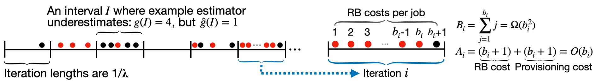
Figure 3: Time moves from left to right in this without-latency example. (Left) Time is partitioned into iterations of length $1/\lambda$ by the example estimator in Section 4.1, and good jobs arrive via a Poisson process with parameter $\lambda$. Black circles denote good jobs, red circles denote bad. An example interval, $\mathcal{I}$, in the third iteration shows possible deviation in $g(\mathcal{I})$ and $\hat{g}(\mathcal{I})$. (Right) A blowup of iteration $i$, with $b_{i}$ bad jobs followed by $1$ good job. The adversary’s and algorithm’s cost is $B_{i}$ and $A_{i}$, respectively. As described in the text, the adversary’s cost is $\Omega(b^{2}_{i})$ and the algorithm’s cost is $O(b_{i})$

With Latency. When there is communication latency between the server and the clients, jobs may submit multiple RB solutions over time. If the submitted solution hardness is less than the threshold, the job request is denied. When this happens, we say that the corresponding job is bounced (see Figure 4). Alternatively, if the hardness of the RB solution exceeds the threshold, then the job overpays.

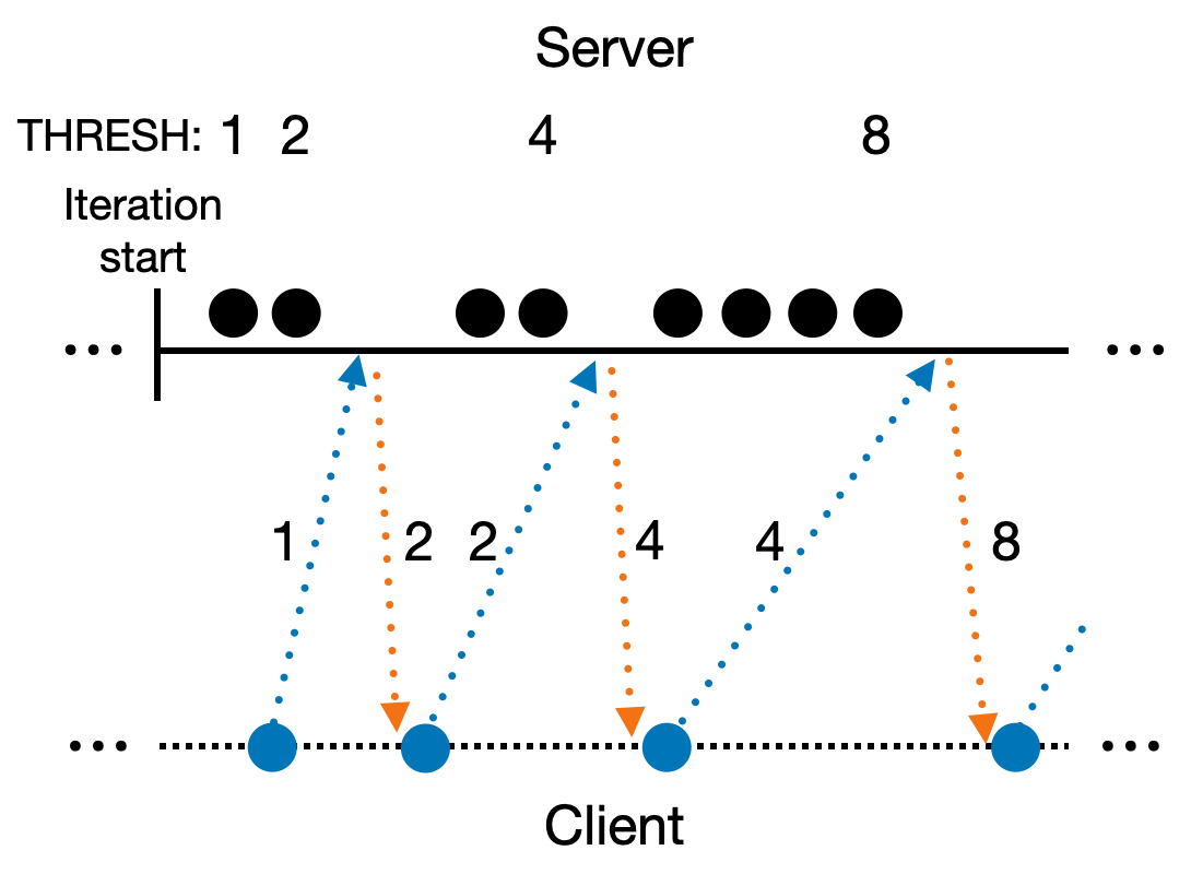
Figure 4: The blue circle is a job that is repeatedly bounced, the black circles are other serviced jobs. The arrows represent the communication from the server to the client of the THRESH value, and from the client to the server of the RB solution value. The blue job is bounced $4$ times and pays a cost of $1+2+4+8$ in the figure.

Now, assume our example estimator, so that iterations end at the same time as the without latency case above. Further, assume a simple distribution for job where exactly $1$ job is generated per iteration at some uniformly distributed time.

Note that $M$ is determined by the maximum latency $L$, and $\lambda$. If the latency $L$ is much larger than $1/\lambda$, then the adversary can delay messages so that $M=L/\lambda$ good jobs, bounced from the previous $L/\lambda$ iterations, are received in the current iteration. The first $M/2$ of these jobs are serviced, driving up the value of THRESH to at least $M/2$. During this time while the remaining jobs are bounced up to $\log(M/2)$ times. Thus, the total cost to the algorithm is $\Omega((g/M)(M^{2}))=\Omega(gM)$.

For these jobs $i=2,...,(M-1)$, the adversary can cause the $i$-th job to bounce $\lfloor{\lg(M-i)}\rfloor$ times with payments of $2^{j}$, for $j=0,...,\lfloor{\lg(M-i)}\rfloor$ in the current iteration. Thus, the total cost to the algorithm is $\Omega((g/M)(M^{2}))=\Omega(gM)$.

5 Analysis of LINEAR

In this section, we formally analyze a general class of algorithms that define iterations like LINEAR, but charge the $i$-th job in the iteration an RB cost of $i^{\alpha}$, for some positive $\alpha$. Our analysis shows that LINEAR, which sets $\alpha=1$, is asymptotically optimal across this class of algorithms.

Let $b$ be the total number of bad jobs, and recall that $g$ is the number of good jobs. We note that all good jobs pay a cost of at most $1$ before they learn the current value of THRESH, which incurs a total cost of $O(g)$. This is asymptotically equal to the total provisioning cost. Thus, for simplicity, in this section, we only count the RB costs for the RB solutions submitted when the jobs are serviced. Throughout, we let $\log(\cdot)$ denote the logarithm base $2$.

Lemma 1.

The number of iterations is no more than $\gamma(g+1)$.

Proof.

Let $\ell$ be the total number of iterations. For all $j$, $1\leq j\leq\ell$, let $\mathcal{I}_{j}$ be the time interval spanning the $j$-th iteration, i.e the interval $(t_{0},t_{1}]$ where $t_{0}$ is the time the $j$-th iteration begins and $t_{1}$ is the time the $j$-th iteration ends.

By the algorithm, $\hat{g}({\mathcal{I}_{j}})\geq 1$ for all $j$. Let $\mathcal{I}_{tot}=\cup_{1\leq j\leq\ell}\mathcal{I}_{j}$. Using the additive property of $\hat{g}$, we get $\hat{g}(\mathcal{I}_{tot})=\sum_{1\leq j\leq\ell}\hat{g}(\mathcal{I}_{j})\geq\ell$. But by our definition of $\gamma$, we know that $\hat{g}(\mathcal{I}_{tot})\leq\gamma(g(\mathcal{I}_{tot})+1)=\gamma(g+1)$. Thus, $\ell\leq\gamma(g+1)$. ∎

Lemma 2.

The number of good jobs serviced in any iteration is no more than $\gamma(\gamma+1)$.

Proof.

Fix some iteration that starts at time $t_{0}$ and ends at time $t_{1}$. Let $\mathcal{I}=[t_{0},t_{1}]$ be the interval associated with that iteration. Let $\mathcal{I}^{\prime}=[t_{0},t_{1}-\epsilon]$ where $\epsilon\geq 0$ is half the amount of time elapsed between $t_{1}$ and the time the server receives the second to last job request of the iteration. First, by construction of $\mathcal{I}^{\prime}$, we have

$$g(\mathcal{I}^{\prime})\geq g(\mathcal{I})-1$$ (1)

Then, by the $\gamma$ estimation gap for $\hat{g}$ on the input, we know that $g(\mathcal{I}^{\prime})\leq\gamma(\hat{g}(\mathcal{I}^{\prime})+\gamma)$. Plugging in the fact that $\hat{g}(\mathcal{I}^{\prime})<1$, which holds by the properties of LINEAR, we get:

$$g(\mathcal{I}^{\prime})<\gamma+\gamma^{2}$$ (2)

Putting together equations 1 and 2, and noting that both $\gamma$ and $g(\mathcal{I})$ are both integers, we get that $g(\mathcal{I})\leq\gamma+\gamma^{2}$. ∎

Lemma 3.

The number of iterations is at least $\max\left(1,\frac{g-\gamma^{2}}{3\gamma^{4}}\right)$.

Proof.

Let $\mathcal{I}_{j}$ be the interval spanning iteration $j$ for $1\leq j\leq\ell$, where $\ell$ is the total number of iterations. By Lemma 2, $g(\mathcal{I}_{j})\leq\gamma(\gamma+1)$ for all $j$. By the estimation gap for $\hat{g}$ on the input, we get $\hat{g}(\mathcal{I}_{j})\leq\gamma g(\mathcal{I}_{j})+\gamma$. Combining these two inequalities, we get $\hat{g}(\mathcal{I}_{j})\leq\gamma^{3}+\gamma^{2}+\gamma$.

Let $\mathcal{I}_{tot}=\cup_{1\leq j\leq\ell}\mathcal{I}_{j}$. Using the additive property of $\hat{g}$, we get

$$\hat{g}(\mathcal{I}_{tot})=\sum_{1\leq j\leq\ell}\hat{g}(\mathcal{I}_{j})\leq(\gamma^{3}+\gamma^{2}+\gamma)\ell.$$

Also, by the estimation gap for $\hat{g}$ on the input, we have $\hat{g}(\mathcal{I}_{tot})\geq g(\mathcal{I}_{tot})/\gamma-\gamma$. Thus,

$$\ell\geq(g/\gamma-\gamma)/(\gamma^{3}+\gamma^{2}+\gamma)=(g-\gamma^{2})/\gamma(\gamma^{3}+\gamma^{2}+\gamma)$$

which proves the lemma. ∎

Recall that $B$ is the cost to the adversary.

Lemma 4.

For any positive $\alpha$, $B\geq\frac{(b-\gamma(g+1))^{\alpha+1}}{(\alpha+1)(\gamma(g+1))^{\alpha}}$.

Proof.

The cost to the adversary is minimized when the bad jobs in each iteration occur before the good jobs. Furthermore, this cost is minimized when the bad jobs are distributed as uniformly as possible across iterations. To see this, assume $j$ jobs are distributed non-uniformly among $\ell$ iterations. Thus, there exists at least one iteration $i_{1}$ with at least $\left\lceil j/\ell\right\rceil+1$ bad jobs, and also at least one iteration $i_{2}$ with at most $\left\lfloor j/\ell\right\rfloor-1$. Since the cost function $i^{\alpha}$ is monotonically increasing, moving one bad job from iteration $i_{1}$ to iteration $i_{2}$ can only decrease the total cost.

To bound the adversarial cost in an iteration, we use an integral lower bound. Namely, for any $x$ and $\alpha$, $\sum_{i=1}^{x}i^{\alpha}\geq 1+\int_{i=1}^{x}i^{\alpha}\,di\geq\frac{x^{\alpha+1}}{\alpha+1}$, where the last inequality holds for $\alpha\geq 0$. If the number of iterations is $\ell>0$, we let $x=\left\lfloor b/\ell\right\rfloor$ in the above and bound the total cost of the adversary as:

$$B \geq\frac{\ell}{\alpha+1}{\left\lfloor\frac{b}{\ell}\right\rfloor^{\alpha+1}}$$

$$\geq\frac{\ell}{\alpha+1}\left(\frac{b}{\ell}-1\right)^{\alpha+1}$$

$$\geq\frac{b-\ell}{\alpha+1}\left(\frac{b}{\ell}-1\right)^{\alpha}$$

$$\geq\frac{b-\gamma(g+1)}{\alpha+1}\left(\frac{b-\gamma(g+1)}{\gamma(g+1)}\right)^{\alpha}$$

$$\geq\frac{(b-\gamma(g+1))^{\alpha+1}}{(\alpha+1)(\gamma(g+1))^{\alpha}}$$

The second step holds since $(b/\ell)-1=(b-\ell)/\ell$. The fourth step holds since, by Lemma 1, $\ell\leq\gamma(g+1)$. ∎

Recall that the cost to the total algorithm is the sum of its RB cost and the provisioning cost. In the following, let $A_{RB}$ denote the RB cost to the algorithm.

Lemma 5.

For $\alpha\geq 1$,

$$A_{RB}=O\left(\gamma^{2\alpha}g+\gamma^{2}b^{\alpha}\right).$$

For $0\leq\alpha<1$,

$$A_{RB}=O\left(\gamma^{2\alpha+4}g+\frac{\gamma^{4\alpha}b^{\alpha+1}}{\max\{1,(g-\gamma^{2})^{\alpha}\}}\right).$$

Proof.

Let $\ell$ be the last iteration with some positive number of good jobs, and for $i\in[1,\ell]$ let $g_{i}$ and $b_{i}$ be the number of good and bad jobs in iteration $i$, respectively. Then the RB cost to the algorithm in an iteration is maximized when all good jobs come at the end of the iteration. For a fixed iteration $i$, the cost is: $\sum_{j=1}^{g_{i}}(b_{i}+j)^{\alpha}$. Then, the total RB cost of the algorithm, $A_{\mbox{\tiny RB}}$ is:

$$\sum_{i=1}^{\ell}\sum_{j=1}^{g_{i}}(b_{i}+j)^{\alpha}$$

Note that for all $1\leq i\leq\ell$, $g_{i}\leq\gamma^{2}+\gamma$, by Lemma 2. For simplicity of notation, in this proof, we let $\beta=\gamma^{2}+\gamma$; and note that for all $i\in[1,\ell]$, $g_{i}\leq\beta$.

We use exchange arguments to determine the settings for which $A_{\mbox{\tiny RB}}$ is maximized subject to our constraints. Consider any initial setting of $\vec{g}$, $\vec{b}$. We assume, without loss of generality, that the $b_{i}$ values are sorted in decreasing order, since if this is not the case, we can swap iteration indices to make it so, without changing the function output.

Good jobs always packed left. We first show that $A_{\mbox{\tiny RB}}$ is maximized when the good jobs are “packed left”: $\beta$ good jobs in each of the first $\left\lfloor g/\beta\right\rfloor$ iterations, and $g\bmod\beta$ good jobs in the last iteration.

To see this, we first claim that, without decreasing $A_{\mbox{\tiny RB}}$, we can rearrange good jobs so that the $g_{i}$ values are non-increasing in $i$. In particular, consider any two iterations $j,k$ such that $1\leq j<k\leq\ell$, where $g_{j}<g_{k}$. We move the last $g_{k}-g_{j}$ good jobs in iteration $k$ to the end of iteration $j$. This will not decrease $A_{\mbox{\tiny RB}}$ since the cost incurred by each of these moved jobs can only increase, since $b_{j}\geq b_{k}$, and our RB-cost function can only increase with the job index in the iteration. Repeating this exchange establishes the claim.

Next, we argue that, without decreasing $A_{\mbox{\tiny RB}}$, we can rearrange good jobs so that the $g_{i}$ values are $\beta$ for all $1\leq i<\ell$. To see this, consider the case where there is any iteration before the last that has less than $\beta$ good jobs, and let $j$ be the leftmost such iteration with $g_{j}<\beta$. Since $j<\ell$, there must be some iteration $k$, where $j<k$, such that $g_{k}>0$. We move the last good job from iteration $k$ to the end of iteration $j$. This will not decrease $A_{\mbox{\tiny RB}}$ since the cost incurred by this moved job can only increase, since our RB-cost function can only increase with the job index in the iteration. Repeating this exchange establishes the claim.

Analyzing $\Delta_{i}$. Next, we set up exchange arguments for the bad jobs. For any integer $x$, define

$$\Delta(x)=\sum_{j=1}^{\beta}(x+1+j)^{\alpha}-\sum_{j=1}^{\beta}(x+j)^{\alpha}$$

If we consider swapping a single bad job from iteration $k$ into iteration $i$ where $1\leq i<k\leq\ell$, this results in the following change in the overall cost: $\Delta(b_{i})-\Delta(b_{k}-1)$.

Let $f:\mathbb{R}\rightarrow\mathbb{R}$ such that, $f(x)=\sum_{j=1}^{\beta}(x+j)^{\alpha}$. For any $i\in[1,\ell]$, this function is continuous when $x\in[b_{i},b_{i}+1]$ and differentiable when $x\in(b_{i},b_{i}+1)$, since it is the sum of a finite number of continuous and differentiable functions respectively. For any $i\in[1,\ell]$, by applying the Mean Value Theorem for the interval $[b_{i},b_{i}+1]$, we have:

$$\Delta(b_{i}) =\frac{f(b_{i}+1)-f(b_{i})}{(b_{i}+1)-b_{i}}=f^{\prime}(x_{i})\mbox{~{}for some~{}}x_{i}\in[b_{i},b_{i}+1].$$

Bad jobs packed left when $\alpha\geq 1$. When $\alpha\geq 1$, $f$ is convex. Hence, $f^{\prime}(x)$ is non-decreasing in $x$. Using this fact and the Mean Value Theorem analysis above, we get that $\Delta(b_{i})\geq f^{\prime}(b_{i})$; and, for any $i<k\leq\ell$, $\Delta(b_{k}-1)\leq f^{\prime}(b_{k})$. In addition, $f^{\prime}(b_{i})\geq f^{\prime}(b_{k})$ since $b_{i}\geq b_{k}$, by our initial assumption that the $b_{i}$ values are non-increasing in $i$. Thus, $\Delta(b_{i})-\Delta(b_{k}-1)\geq 0$.

This implies that $A_{\mbox{\tiny RB}}$ does not decrease whenever we move a bad job from some iteration with index $k>1$ to iteration $i=1$. Hence, $A_{RB}$ is maximized when all bad jobs occur in the first iteration.

Bad jobs evenly spread when $\alpha<1$. When $\alpha<1$, $f$ is concave. Hence, $f^{\prime}(x)$ is non-increasing in $x$. Using this fact and the Mean Value Theorem analysis above, we get that $\Delta(b_{i})\leq f^{\prime}(b_{i})$; and, for any $1<k\leq\ell$, $\Delta(b_{k}-1)\geq f^{\prime}(b_{k})$. In addition, $f^{\prime}(b_{k})\geq f^{\prime}(b_{i})$ since $b_{i}\geq b_{k}$, by our initial assumption that the $b_{i}$ values are non-increasing in $i$. Thus, $\Delta(b_{i})-\Delta(b_{k}-1)\leq 0$.

This implies that $A_{\mbox{\tiny RB}}$ increases whenever we swap bad jobs from an iteration with a larger number of bad jobs to an iteration with a smaller number. Hence, $A_{\mbox{\tiny RB}}$ is maximized when bad jobs are distributed as evenly as possible across iterations.

Upper bound on $A_{RB}$. We can now bound $A_{\mbox{\tiny RB}}$ via a case analysis.

Case $\alpha\geq 1$: With the above exchange argument in hand, we have:

$$A_{RB} \leq\left(\frac{g}{\beta}\right)\sum_{j=1}^{\beta}j^{\alpha}+\sum_{j=1}^{\min(\beta,g)}(b+j)^{\alpha}$$

$$\leq\left(\frac{g}{\beta}\right)\sum_{j=1}^{\beta}j^{\alpha}+\min(\beta,g)(b+\beta)^{\alpha}$$

$$\leq 2\left(\frac{g}{\beta}\right)\frac{\beta^{\alpha+1}}{\alpha+1}+\min(\beta,g)(b+\beta)^{\alpha}$$

$$\leq 2\left(\frac{g}{\beta}\right)\frac{\beta^{\alpha+1}}{\alpha+1}+\beta(2b)^{\alpha}+g(2\beta)^{\alpha}$$

$$=O\left(\beta^{\alpha}g+\beta b^{\alpha}\right)$$

where the third line follows by upper bounding the sum by an integral, and the fourth line follows from the inequality $(x+y)^{d}\leq(2x)^{d}+(2y)^{d}$ for any positive $x,y$, and $d$, which holds because $x+y\leq 2x$ or $x+y\leq 2y$. Finally, note that replacing $\beta$ with $\gamma^{2}+\gamma\leq 2\gamma^{2}$ gives the same asymptotic upper bound in the lemma statement.

Case $\alpha<1$: With the above exchange argument in hand, we have:

$$A_{RB} \leq\ell\sum_{j=1}^{\beta}(b/\ell+j)^{\alpha}$$

$$\leq\ell\sum_{j=1}^{\beta+b/\ell+1}j^{\alpha}$$

$$\leq 2\ell\frac{(\beta+b/\ell+1)^{\alpha+1}}{\alpha+1}$$

$$\leq 2\ell\frac{(2\beta+2)^{\alpha+1}+(2b/\ell)^{\alpha+1}}{\alpha+1}$$

$$=O\left(\gamma^{2\alpha+4}g+\frac{\gamma^{4\alpha}b^{\alpha+1}}{\max\{1,(g-\gamma^{2})^{\alpha}\}}\right)$$

In the above, the last line follows by Lemma 3, and noting that $1/\alpha$ is a fixed constant. ∎

Note from Lemma 5 that for $b\geq\gamma^{2}$, $A_{\mbox{\tiny RB}}$ is minimized when $\alpha\geq 1$. Using this fact, we show $\alpha=1$ minimizes the total cost of the algorithm as a function of $B$ and $g$. The following theorem bounds the RB cost of the algorithm for that case.

Lemma 6.

The total cost to LINEAR is $O\left(\gamma^{5/2}\sqrt{B(g+1)}+\gamma^{3}(g+1)\right)$.

Proof.

To bound the cost of A, we perform a case analysis.

Case: $b\geq 2\gamma(g+1)$. In this case, $\gamma(g+1)\leq b/2$. By Lemma 4, we have:

$$B\geq\frac{(b-\gamma(g+1))^{\alpha+1}}{(\alpha+1)(\gamma(g+1))^{\alpha}}\geq\frac{(b/2)^{\alpha+1}}{(\alpha+1)(\gamma(g+1))^{\alpha}}=\frac{b^{\alpha+1}}{2^{\alpha+1}(\alpha+1)\gamma^{\alpha}(g+1)^{\alpha}}$$

The provisioning cost is $b+g\leq 2b$, since in this case $g\leq b/(2\gamma)\leq b/2$. Let $A$ denote the total cost to the algorithm. We now use Lemma 5; specifically, the case for $\alpha\geq 1$, which gives the smallest worst case RB cost to the algorithm, across all values of $g$ and $b$ and $\gamma$. This yields:

$$A\leq 2b+c(\gamma^{2\alpha}g+\gamma^{2}b^{\alpha})$$

where $c>0$ is a sufficiently large constant. Thus we have:

$$A \leq 2b+c(\gamma^{2\alpha}g+\gamma^{2}b^{\alpha})$$

$$\leq 2b+c(\gamma^{2\alpha}(b/2\gamma)+\gamma^{2}b^{\alpha})$$

$$\leq 2b+c(\gamma^{2\alpha-1}b+\gamma^{2}b^{\alpha})$$

Where the second line holds since $\gamma(g+1)\leq b/2$ implies that $\gamma g\leq b/2$, or $g\leq b/(2\gamma)$. Note that the above is minimized over the range $\alpha\geq 1$, when $\alpha=1$. In this case, we have:

$$A\leq 2b+c\left(\gamma b+\gamma^{2}b\right)\leq(c\gamma+\gamma^{2}+2)b=O\left(\gamma^{5/2}\sqrt{B(g+1)}\right).$$

In the equality above, for $\alpha=1$, $B\geq\frac{b^{2}}{8\gamma(g+1)}$, which implies that $b\leq\sqrt{8\gamma B(g+1)}$.

Case: $b<2\gamma(g+1)$. In this case, the provisioning cost is $g+b\leq(2\gamma+1)(g+1)$. So when $\alpha=1$, we can bound the total cost as:

$$A\leq(2\gamma+1)(g+1)+c(\gamma^{2}g+\gamma^{2}b)\leq(2\gamma+1)(g+1)+c(\gamma^{2}g+\gamma^{2}(2\gamma(g+1)))=O(\gamma^{3}(g+1))$$

which completes the proof. ∎

The communications bounds for LINEAR are straightforward.

Lemma 7.

In LINEAR, the server sends $O(g)$ messages to clients, and clients send a total of $O(g)$ messages to the server. Also, each good job is serviced after an exchange of at most $3$ messages between the client and server

Proof.

Since there is no latency, each client immediately receives the current value of THRESH if its first message to the server has an RB solution with value too small. Then, on the second attempt the client attaches a RB solution with the correct value, and so receives service. Hence, each good job is serviced with at most $2$ messages from client to server and at most $1$ message from server to client. ∎

The proof of Theorem 1.1 now follows directly from Lemmas 6 and 7.

6 Analysis of LINEAR-POWER

How much do RB costs increase for LINEAR-POWER in our harder with-latency problem variant (recall Section 1.1)? We say that a good job “overpays” if the RB cost submitted when the job is serviced exceeds the cost that the server expects. In this section, we bound the total amount overpaid by all good jobs in the with-latency model. When compared to LINEAR, the adversary cost in LINEAR-POWER decreases by at most a factor of $2$; and the total amount spent by good jobs that do not overpay increases by at most a factor of $2$. Thus, overpayment is the only possible source of asymptotic increase in algorithmic costs.

Thus we upper bound the overpayment amount. To do this, we partition time into epochs. An epoch is a contiguous time interval ending with a period of $2L$ seconds, where the RB threshold during the entire period never increases.

In the following, for all $i\geq 1$, let $B_{i}$ be the amount spent by the adversary in epoch $i$. For convenience, we define $B_{0}=0$.

Lemma 8.

For all $i\geq 1$, the maximum RB threshold value in epoch $i$ is at most

$$2\gamma^{2}\max\left(1,2\sqrt{B_{i}}\right)\leq 4\gamma^{2}\sqrt{B_{i}+1}$$

Proof.

Fix an epoch $i\geq 1$ and let $2^{x}$ be the maximum RB threshold in that epoch.

If $B_{i}>0$, and the epoch consists solely of bad jobs, we know that $B_{i}\geq 2^{2(x-1)}$, because of the way that our server increases the threshold. Hence, the bad jobs contribute no more than $((1/2)\log B_{i})+1$ to the value $x$, when $B_{i}>0$.

In any period where the RB threshold monotonically increases, the number of good jobs is no more than the number of good jobs in an iteration, which is at most $\gamma(\gamma+1)\leq 2\gamma^{2}$ by Lemma 2. Thus, the total increase in $x$ from good jobs is at most $\log 2\gamma^{2}$.

Putting these together, we get that when $B_{i}=0$, $x\leq\log 2\gamma^{2}$ and when $B_{i}>0$, $x\leq(1/2\log B_{i})+1+\log 2\gamma^{2}$. Hence the maximum RB threshold value is at most $2\gamma^{2}\max(1,2\sqrt{B_{i}})\leq 4\gamma^{2}\sqrt{B_{i}+1}$. ∎

Lemma 9.

For all $i\geq 1$, at most $4M(\log(\gamma(B_{i}+1))+1)$ good jobs arrive in epoch $i$.

Proof.

Over every $2L$ seconds, starting from the beginning of the epoch, the RB threshold value must double, or else the epoch will end. Thus, the epoch lasts at most $2L(x+1)$ seconds, where $2^{x}$ is the maximum RB threshold achieved in that epoch.

By Lemma 8, $2^{x}\leq 4\gamma^{2}\sqrt{B_{i}+1}$; taking the log and simplifying, we get $x\leq 2+2\log(\gamma(B_{i}+1))$. The lemma follows since over a period of $2L$ seconds, at most $2M$ good jobs can arrive. ∎

Lemma 10.

Any epoch has overpaying jobs only if either the epoch or its preceding epoch spans the beginning of some iteration.

Proof.

All jobs entering prior to the last $2L$ seconds of an epoch are serviced before the end of the epoch, since, by definition, the RB threshold value is non-increasing during those $2L$ seconds. Thus, all jobs serviced in some fixed epoch either have entered during that epoch or entered in the final $2L$ seconds of the preceding epoch.

If neither the current epoch nor the preceding epoch spanned the beginning of an iteration, then the RB threshold never resets to $1$ during the lifetime of any of these jobs. So the RB threshold is non-decreasing during each such job’s lifetime. Thus, none of the jobs can ever have an attached RB value that is larger than the RB threshold, and so no overpayment occurs. ∎

Lemma 11.

For all $i\geq 1$, the total amount that good jobs overpay in epoch $i$ is at most $8M\gamma^{2}(\sqrt{B_{i-1}}+\sqrt{B_{i}}+1)(\log(\gamma(B_{i}+1))+2)$.

Proof.

First, note that every good job serviced in epoch $i$ either arrived in epoch $i$: at most $4M(\log(\gamma(B_{i}+1)+1)$ such jobs by Lemma 9; or arrived in the last $2L$ seconds of the preceding epoch: at most $2M$ such jobs. Thus, there are at most $4M(\log(\gamma(B_{i}+1))+2)$ good jobs serviced in epoch $i$.

By Lemma 8, the maximum RB threshold value in either epoch $i$ or $i-1$ is:

$$2\gamma^{2}\max\left\{\sqrt{B_{i-1}},\sqrt{B_{i}},1\right\}\leq 2\gamma^{2}\left(\sqrt{B_{i-1}}+\sqrt{B_{i}}+1\right)$$

This is the maximum amount that any job serviced in epoch $i$ can overpay. Multiplying by the number of good jobs serviced, we obtain the bound in the lemma statement. ∎

Lemma 12.

The total amount overpaid by good jobs in LINEAR-POWER is

$$O\left(M\log(\gamma(B+2))\left(\gamma^{5/2}\sqrt{(g+1)B}+\gamma^{3}(g+1)\right)\right)$$

Proof.

Let $X$ be the total amount overpaid by good jobs in LINEAR-POWER. We will give two upperbounds on $X$ and then combine them.

First, by Lemma 8 and the fact that for all $i\geq 1$, $B_{i}\leq B$, we know that the maximum RB cost any good job can over pay is at most $4\gamma^{2}\sqrt{B+1}$. Multiplying by all good jobs, we get:

$$X\leq 4(g+1)\gamma^{2}\sqrt{B+1}$$ (3)

Next, let $S$ be the set of indices of epochs that have overpaying jobs. Then, by Lemma 11:

$$X \leq\sum_{j\in S}8M\gamma^{2}(\sqrt{B_{i-1}}+\sqrt{B_{i}}+1)(\log(\gamma(B_{i}+1))+2)$$

$$\leq 8M\gamma^{2}(\log(\gamma(B+1))+2)\sum_{j\in S}(\sqrt{B_{j-1}}+\sqrt{B_{j}}+1)$$

$$\leq 8M\gamma^{2}(\log(\gamma(B+1))+2)\left(|S|+\sum_{j\in S}\sqrt{B_{j-1}}+\sum_{j\in S}\sqrt{B_{j}}\right)$$

$$\leq 8M\gamma^{2}(\log(\gamma(B+1))+2)\left(|S|+2\sqrt{B}\left(\min(\sqrt{S},\sqrt{B})\right)\right)$$

In the above, the fourth step holds by noting that the sum of the $B_{j-1}$ and $B_{j}$ terms are both at most $B$, applying Cauchy-Schwartz to both sums, and noting that the sum of the $\sqrt{B_{i}}$ can never be larger than $B$.

Next, noting that $|S|\leq 2\gamma(g+1)$ by Lemmas 1 and 10, we have for some constant $C$:

$$X\leq CM\gamma^{2}\left(\gamma(g+1)+\sqrt{B}\left(\min(\sqrt{\gamma(g+1)},\sqrt{B}\right)\log(\gamma(B+2)))\right)$$ (4)

Putting together equations 3 and 4, we have

$$X =O\left(\gamma^{2}\sqrt{B+1}\min\left(g+1,M\log(\gamma(B+2))\left(\min(\sqrt{\gamma(g+1)},\sqrt{B+1})\right)\right)\right)$$

∎

Lemmas 13, 14, and 15 below complete the proof of our second main result, Theorem 1.2.

Lemma 13.

LINEAR-POWER has total cost:

$$\tilde{O}\left(\gamma^{3}\left(\sqrt{B+1}\min\left(g+1,M\sqrt{g+1},M\sqrt{B+1}\right)+(g+1)\right)\right).$$

Proof.

Fix the order in which jobs are serviced by LINEAR-POWER. The threshold value when a job is serviced in LINEAR-POWER will differ by at most a factor of $2$ from LINEAR because of the fact that LINEAR-POWER uses powers of $2$. Thus, the total amount spent by the adversary decreases by at most a factor of $2$, and the total amount spent by the algorithm on all jobs that do not overpay increases by at most a factor of $2$. It follows that the asymptotic results in Theorem 1.1 hold, except for the costs due to overpayment by the good jobs.

So, we can bound the asymptotic cost of the algorithm as the cost from LINEAR plus the cost due to overpayment. The cost in the theorem statement is the asymptotic sum of the costs from Theorem 1.1: and from Lemma 12. This is

$$O\mbox{\Large(}\gamma^{2}\sqrt{B+1}\min\mbox{\Large(}g+1,M\log(\gamma(B+2))\mbox{\Large(}\min(\sqrt{\gamma(g+1)},\sqrt{B+1}))\mbox{\Large)}\mbox{\Large)}+\gamma^{5/2}\sqrt{B(g+1)}+\gamma^{3}(g+1)\mbox{\Large)}$$

which is

$$\tilde{O}\left(\gamma^{3}\left(\sqrt{B+1}\min\left(g+1,M\sqrt{g+1},M\sqrt{B+1}\right)+(g+1)\right)\right)$$

which completes the argument. ∎

Lemma 14.

The maximum time for any good job to begin service is $L(4\log(\gamma(B+1))+3)$ seconds.

Proof.

Fix any good job. Every time the job is bounced, the threshold value sent from the server to the corresponding client at least doubles. The client receives the new threshold value from the server within $L$ seconds.

How many times can the RB threshold value change? If $B>0$, the number of times that bad jobs can double the RB threshold is at most $(1/2)\log B$. By Lemma 2, the number of good jobs in an iteration is at most $\gamma(\gamma+1)\leq 2\gamma^{2}$. Hence the total number of times the RB threshold can change for $B=0$ is most $1+2\log\gamma$; and for $B>0$, at most $1+2\log\gamma+(1/2)\log B$. In both cases, this is at most $1+2\log\gamma+(1/2)\log(B+1)\leq 1+2\log(\gamma(B+1))$.

Every time the job is bounced takes at most $2L$ seconds: $L$ seconds to send the job to the server, and $L$ seconds to receive the new RB threshold from the server. When the job is serviced it takes at most $L$ seconds: the time to send the job to the server. Thus, the total time for the job to be serviced is at most $2L(2\log(\gamma(B+1))+1)+L\leq L(4\log(\gamma(B+1))+3)$. ∎

The following lemma bounds the number of messages sent from the server to clients and from clients to the server. Note that the adversary can cause the server to send a message to it for every request that it sends.

Lemma 15.

In LINEAR-POWER the server sends $O(g\log(B+(2\gamma^{2})))$ messages to clients, and clients send a total of $O(g\log(B+2\gamma^{2}))$ messages to the server.

Proof.

Every time the server sends a message to the client, the threshold value sent to that client must at least double. How often can this happen? By Lemma 2 the number of good jobs in any iteration is at most $\gamma(\gamma+1)\leq 2\gamma^{2}$. So, the total number of changes to the threshold value in any iteration is $\log(B+(2\gamma^{2}))$. So the maximum threshold value ever achieved is at most $2^{\log(B+(2\gamma^{2}))}$. Hence, the maximum number of messages sent to any client is $O(\log(B+(2\gamma^{2})))$. It follows that the total number of messages sent to clients is $O(g\log(B+(2\gamma^{2})))$

Every time a client sends a new message to the server, the RB value appended to that message doubles. The maximum threshold value set by the server over all iterations is at most $\log(B+2\gamma^{2})$, and so a good job will send at most that number of messages. Hence, all the $g$ good jobs send a total of $O(g\log(B+2\gamma^{2}))$ messages to the server. ∎

7 Lower Bound

In this section we give a lower bound for randomized algorithms for our problem without latency. This lower bound also directly holds for our harder with-latency variant of our model.

7.1 Our Adversary

Let $\gamma$ be any positive integer, $g_{0}$ be any multiple of $\gamma$, and $n$ be any multiple of $g_{0}\gamma$. To prove our lower bound, we choose both an input distribution and also a specific estimator.

Distribution. There are two possible distributions of $n$ jobs. In both distributions, the jobs are evenly spread in a sequence over $T$ seconds for any value $T$; in particular, the $i$-th job occurs at time $T(i/n)$.

In distribution one, the number of good jobs is $g_{1}=\gamma g_{0}$. In distribution two, it is $g_{2}=g_{0}/\gamma$. Our adversary chooses one of these two values, each with probability $1/2$.

Then, for $i\in\{1,2\}$, we partition from left to right the sequence of jobs into contiguous subsequences of length $n/g_{i}$. In each partition, we set one job selected uniformly at random to be good, and the remaining jobs to be bad.

Estimator. For any interval $\mathcal{I}$, let $\textit{num}(\mathcal{I})$ be the number of (good and bad) jobs overlapped by $\mathcal{I}$, i.e. $\textit{num}(\mathcal{I})=\mathcal{I}\cap\{k(T/n):k\in\mathbb{Z}^{+}\}$. Then

$$\hat{g}(\mathcal{I})=(g_{0}/n)\textit{num}(\mathcal{I})$$

It is easy to verify that the above function always has the additive property, and so is an estimator. Moreover, this estimator has two important properties. First, the estimation gap is always at most $\gamma$ for either input distribution (see Lemma 16). Second, it is independent of the choice of distribution one or two.

7.2 Analysis

We first show that this estimator has $\gamma$ estimation gap for both distributions.

Lemma 16.

For both distributions, for any interval $\mathcal{I}$, we have:

$$g(\mathcal{I})/\gamma-\gamma\leq\hat{g}(\mathcal{I})\leq\gamma g(\mathcal{I})+\gamma$$

Proof.

Let $g_{\max}=\max\{g_{1},g_{2}\}=\gamma g_{0}$ and $g_{\min}=\min\{g_{1},g_{2}\}=g_{0}/\gamma$, and fix any interval $\mathcal{I}$. Then, for each distribution we have the following based on the observation that there is one good job in every partition of size $n/g_{i}$ for $i\in\{1,2\}$

$$g(\mathcal{I})\leq\lceil\textit{num}(\mathcal{I})/(n/g_{i})\rceil\leq\left(\frac{g_{\max}}{n}\right)\textit{num}(\mathcal{I})+1\leq\left(\frac{\gamma g_{0}}{n}\right)\textit{num}(\mathcal{I})+1.$$ (5)

Thus:

$$\left(\frac{1}{\gamma}\right)g(\mathcal{I})-\gamma \leq\left(\frac{1}{\gamma}\right)\left(\frac{\gamma g_{0}}{n}\textit{num}(\mathcal{I})+1\right)-\gamma$$

$$\leq\left(\frac{g_{0}}{n}\right)\textit{num}(\mathcal{I})+\frac{1}{\gamma}-\gamma$$

$$\leq\hat{g}(\mathcal{I})$$

In the above, the first line follows from Equation 5, and the last line follows for $\gamma\geq 1$ and by the properties of our estimator.

For the other direction, note that for any interval $\mathcal{I}$, we have:

$$g(\mathcal{I})\geq\lfloor\textit{num}(\mathcal{I})/(n/g_{i})\rfloor\geq\left(\frac{g_{\min}}{n}\right)\textit{num}(\mathcal{I})-1\geq\left(\frac{g_{0}}{\gamma n}\right)\textit{num}(\mathcal{I})-1.$$ (6)

Thus:

$$\gamma g(\mathcal{I})+\gamma \geq\gamma\left(\frac{g_{0}}{\gamma n}\textit{num}(\mathcal{I})-1\right)+\gamma$$

$$\geq\left(\frac{g_{0}}{n}\right)\textit{num}(\mathcal{I})$$

$$=\hat{g}(\mathcal{I})$$

In the above, the first line follows from Equation 6, and the last line follows from the fact that $\gamma\geq 1$, and the definition of the estimator. Hence, by the above analysis, our estimator has $\gamma$ estimation gap for both distributions. ∎

Since the estimator returns the same outputs on both distributions, any deterministic algorithm will set job costs to be the same. This fact helps in proving the following lemma about expected costs.

Lemma 17.

Consider any deterministic algorithm that runs on the above adversarial input distribution and estimator. Define the following random variables: $A$ is the cost to the algorithm; $B$ is the cost to the adversary; and $g$ is the number of good jobs in the input. Then:

$$E\left(A-\sqrt{Bg\gamma}\right)\geq 0$$

Proof.

By Lemma 16 the estimator has $\gamma$ estimation gap, and returns the exact same values whether the number of actual good jobs is $g_{1}$ or $g_{2}$. Thus, the algorithm can set RB costs based only on the job index. So, for each index $i\in[1,n]$, let $c_{i}$ be the RB cost charged for the $i$-th job; and let $C=\sum_{i=1}^{n}c_{i}$. Let $E_{1}(A)$, $E_{1}(B)$ be the expected algorithmic RB cost and expected adversarial total cost for distribution $1$; and $E_{2}(A)$, $E_{2}(B)$ be analogous expected costs for distribution $2$.

To show $E(A-\sqrt{Bg\gamma})\geq 0$, we will show that $E(A)/\sqrt{E(B)g}\geq\sqrt{\gamma}$, and then cross-multiply and use Jensen’s inequality. If we define a random variable $a_{i}$ that has value $c_{i}$ if the $i$-th job is good and $0$ otherwise, and note that $A=\sum_{i=1}^{n}a_{i}$, then by linearity of expectation, the expected RB cost to the algorithm in distribution $1$ is $\sum_{i=1}^{n}E(a_{i})=C\gamma g_{0}/n$, with an additional provisioning cost of $n$. A similar analysis for $E_{1}(B)$ gives:

$$E_{1}(A) =C\gamma g_{0}/n+n$$

$$E_{1}(B) =\frac{n-\gamma g_{0}}{n}C.$$

Similarly, for the second distribution:

$$E_{2}(A) =Cg_{0}/(\gamma n)+n$$

$$E_{2}(B) =\frac{n-g_{0}/\gamma}{n}C.$$

Hence, we have:

$$\frac{E_{1}(A)}{\sqrt{E_{1}(B)g_{1}}} =\sqrt{\frac{C\gamma g_{0}}{n(n-\gamma g_{0})}}+\sqrt{\frac{n^{3}}{C\gamma g_{0}(n-\gamma g_{0})}}$$

$$=\frac{V_{1}+n/V_{1}}{\sqrt{(n-\gamma g_{0})}}$$

where $V_{1}=\sqrt{\frac{C\gamma g_{0}}{n}}$. and

$$\frac{E_{2}(A)}{\sqrt{E_{2}(B)g_{2}}} =\sqrt{\frac{C(g_{0}/\gamma)}{n(n-g_{0}/\gamma)}}+\sqrt{\frac{n^{3}}{C(g_{0}/\gamma)(n-g_{0}/\gamma)}}$$

$$=\frac{V_{2}+n/V_{2}}{\sqrt{(n-g_{0}/\gamma)}}$$

and where $V_{2}=\sqrt{\frac{Cg_{0}/\gamma}{n}}=V_{1}/\gamma$.

Let $f(C)$ be the expected value of the ratio of $E(A)/\sqrt{E(B)g}$ as a function of $C$. Since the adversary chooses each distribution with probability $1/2$, we have:

$$f(C) =1/2\left(\frac{V_{1}+n/V_{1}}{\sqrt{n-\gamma g_{0}}}+\frac{V_{1}/\gamma+n\gamma/V_{1}}{\sqrt{n-g_{0}/\gamma}}\right)$$

$$\geq\frac{1}{2(\sqrt{n-\gamma/g_{0}})}\left((1+1/\gamma)V_{1}+(1+\gamma)n/V_{1})\right)$$

Consider the expression in parenthesis above: $g(V_{1})=(1+1/\gamma)V_{1}+(1+\gamma)n/V_{1}$ The derivative of $g(V_{1})$ with respect to $V_{1}$ is $1/\gamma+1-(\gamma+1)n/V_{1}^{2}$. From this, we see that $g(V_{1})$ is minimized when $V_{1}=\sqrt{n\gamma}$. Plugging this back in to $f$, we get that $f(C)\geq\sqrt{\gamma}$.

$$f(C) \geq\frac{1}{2(\sqrt{n-\gamma/g_{0}})}\left((1+1/\gamma)V_{1}+(1+\gamma)(n/V_{1}))\right)$$

$$=\frac{1}{2(\sqrt{n-\gamma/g_{0}})}\left(\sqrt{n\gamma}+\sqrt{n/\gamma}+\sqrt{n/\gamma}+\sqrt{n\gamma}\right)$$

$$=\frac{1}{2(\sqrt{n-\gamma/g_{0}})}\left(2\sqrt{n\gamma}+2\sqrt{n/\gamma}\right)$$

$$=\frac{\sqrt{n\gamma}+\sqrt{n/\gamma}}{\sqrt{n-\gamma/g_{0}}}$$

$$\geq\frac{\sqrt{n\gamma}+\sqrt{n/\gamma}}{\sqrt{n}}$$

$$\geq\sqrt{\gamma}$$

Hence, we have proven that the expected value of the ratio $E(A)/\sqrt{E(B)g\gamma}$ is always at least $1$, for our adversarial input distribution, for any deterministic algorithm. Cross multiplying, we get

$$E(A) \geq\sqrt{E(B)g\gamma}$$

$$\geq E(\sqrt{Bg\gamma})$$

where the second line holds by applying Jensen’s inequality [55] to the convex function $f(x)=-\sqrt{x}$. Finally, by linearity of expectation, this inequality implies that $E(A-\sqrt{Bg\gamma})\geq 0$, which completes the argument. ∎

Theorem 1.3. Let $\gamma$ be any positive integer; $g_{0}$ be any positive multiple of $\gamma$; and $n$ any multiple of $\gamma g_{0}$. Next, fix any randomized algorithm in our model. Then, there is an input with $n$ jobs, $g$ of which are good for $g\in\{\gamma g_{0},g_{0}/\gamma\}$; and an estimator with estimation gap $\gamma$ on that input. Additionally, the randomized algorithm on that input has expected cost:

$$E(A)=\Omega\left(E(\sqrt{\gamma B(g+1)})+\gamma(g+1)\right).$$

Proof.

By Lemma 17, on our adversarial distribution, any deterministic algorithm has $E(A)-\sqrt{\gamma E(B)g\gamma}\geq 0$.

We fix values of $g_{0}$, $n$ and $\gamma$ in our adversarial distribution and define a game theoretic payoff matrix $\mathcal{M}$ as follows. The rows of $\mathcal{M}$ correspond to deterministic inputs in the sample space used by our adversarial distribution; the columns correspond to all deterministic algorithms over $n$ jobs. Further, for each input $i$, and algorithm $j$, the matrix entry $\mathcal{M}(i,j)$ is the value $A-\sqrt{Bg\gamma}$, where $A$ and $B$ are the costs to the algorithm and adversary respectively, when algorithm $j$ is run on input $i$; and the value $g$ is the number of good jobs in input $i$.

Lemma 17 proves that the minimax of this payoff matrix is at least $0$. So by Von Neumann’s minimax theorem [61, 79], the maximin is also at least $0$. In other words, via Yao’s principal [79], any randomized algorithm has some deterministic input for which $E(A-\sqrt{\gamma Bg})\geq 0$. By linearity of expectation:

$$E(A) \geq E(\sqrt{\gamma Bg}).$$

Finally, note that every algorithm has job provisioning cost that equals $n=\gamma g$, so $E(A)=n\geq\gamma g$. Adding this to the above inequality gives that $2E(A)\geq E(\sqrt{\gamma Bg})+\gamma g$, or $E(A)=\Omega(\sqrt{\gamma E(B)g}+\gamma g)$. Since $g$ is positive, this is $\Omega\left(\sqrt{\gamma E(B)(g+1)}+\gamma(g+1)\right)$. Since the sample space of our adversarial distribution has $g\in\{\gamma g_{0},g_{0}/\gamma\}$, the worst-case distribution chosen for the maximin will also have $g\in\{\gamma g_{0},g_{0}/\gamma\}$. ∎

8 Simulation Results

We perform experiments for input distributions where there is a large attack and all good jobs are serviced as late as possible; here, our aim is to verify the scaling behavior predicted by theory. Our custom simulations are written in Python and the source code is available to the public via GitHub [16].

8.1 Experiments for LINEAR

In our experiments for LINEAR, the distribution of good and bad jobs, along with the performance of the estimator, is setup as follows. Let the jobs be indexed as $J_{1},J_{2},\ldots,J_{n}$. Then, let $\mathcal{I}_{m}$ be the time interval containing the single point in time at which the $m$-th job is generated for $1\leq m\leq n$.

• For $m\in[1,\gamma]$, job $J_{m}$ is bad and $\hat{g}(\mathcal{I}_{m})=1$

• For $m\in[\gamma+1,n-\gamma]$, job $J_{m}$ is bad and $\hat{g}(\mathcal{I}_{m})=0$

• For $m\in[n-\gamma+1,n-1]$, job $J_{m}$ is good and $\hat{g}(\mathcal{I}_{m})=0$

• For $m=n$, job $J_{m}$ is good and $\hat{g}(\mathcal{I}_{m})=1$

For all other intervals $\mathcal{I}_{t}$ consisting of single points in time, $t$, $\hat{g}(\mathcal{I}_{t})=0$. Then, the additive property defines the estimator output for all larger intervals.

Thus, the first $\gamma$ jobs are bad, but considered to be good by the estimator (each such job will end an iteration); the next $n-2\gamma$ jobs are bad and considered to be bad by the estimator; the next $\gamma-1$ jobs are good and considered to be bad by the estimator; and the last job is good and considered to be good by the estimator (which ends an iteration).

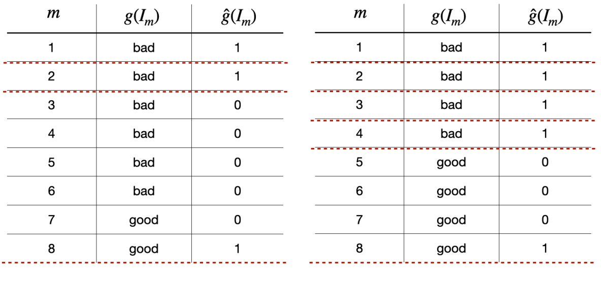
Figure 6: Two small input examples for experiments with LINEAR for $n=8$, with $\gamma=2$ (left) and $\gamma=4$ (right). Red dashed lines indicate the end of an iteration.

We highlight that, in the above setup, the estimator errs in a way that favors the adversary and disfavors our algorithm. Given that the first $\gamma$ bad jobs are (erroneously) considered good by the estimator, the adversary pays only $1$ for each such job, since each such job ends an iteration. Thus, as $\gamma$ grows, the adversary benefits; see the examples for $\gamma=2$ and $\gamma=4$ in Figure 6. Additionally, of the final $\gamma$ (good) jobs, all but the last one are correctly identified as good, which increases the cost to the algorithm.

Specific Experiments. We conduct two experiments. For our first experiment, we let $n=10\times 2^{x}$ for integer $x\in[-1,18]$. Then, we fix $\gamma=1$ and investigate the impact of different values of $\alpha$ (recall Section 5); specifically, we let $\alpha=0,1/2,1$ and $2$.

For our second experiment, we set $n=10\times 2^{x}$, where $x\in[3,18]$. We fix $\alpha=1$ and investigate the impact of different values of $\gamma$; specifically, we let $\gamma=1,2,4,8,16$ and $32$. The range for $x$ is slightly smaller than in the first experiments, since the smallest power-of-$2$-sized input that holds both good and bad jobs is $10\times 2^{3}=80$ when $\gamma=32$.

Results for LINEAR. The results of our first experiment are plotted in Figure 7 (Left). The algorithm’s cost is denoted by $A$, while the adversary’s cost is denoted by $B$. The results show scaling consistent with our theoretical analysis. Notably, setting $\alpha=1$ achieves the most advantageous cost for algorithm versus the adversary. We observe that for $\alpha=0,2$ and $0.5$, the algorithm cost increases by up to a factor of approximately $33.3$, $3.3$, and $1.8$, respectively, relative to LINEAR (i.e., $\alpha=1$) at $B=10^{4}$. We include the line $A=B$ as a reference point, and this closely corresponds to the case for $\alpha=0$ (i.e., each job has cost $1$), since the provisioning cost incurred by the algorithm is close to the number of bad jobs in these experiments. We also include the equation $A=2(\sqrt{B(g+1)}+g)$, which closely fits the line for $\alpha=1$.

The results of our second experiment are plotted in Figure 7 (Right). As expected, when $\gamma$ increases—and, thus, the accuracy of our estimator worsens—the cost ratio of the algorithm to the adversary increases. Specifically, for $B=10^{7}$, we see that the values of $\gamma=2,4,8,16$ and $32$ correspond to a cost ratio that is, respectively, a factor of $1.5$, $2.6$, $4.4$, $8.8$, and $15.5$ larger than than for $\gamma=1$. Given this, and noting the fairly even spacing of the trend lines on the log-log-scaled plot, the cost appears to scale according to a (small) polynomial in $\gamma$. We note that, despite this behavior, the cost of the algorithm versus the adversary is still below the $A=B$ line; thus, LINEAR still achieves a significant advantage for the values of $\gamma$ tested.

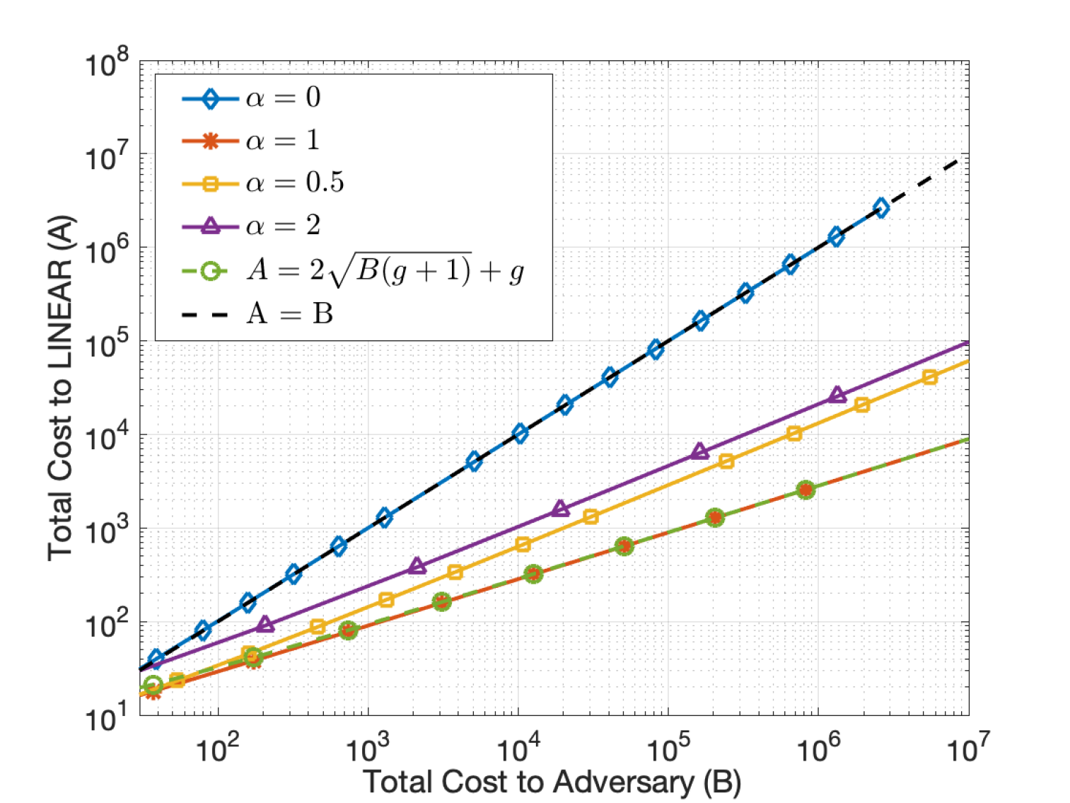
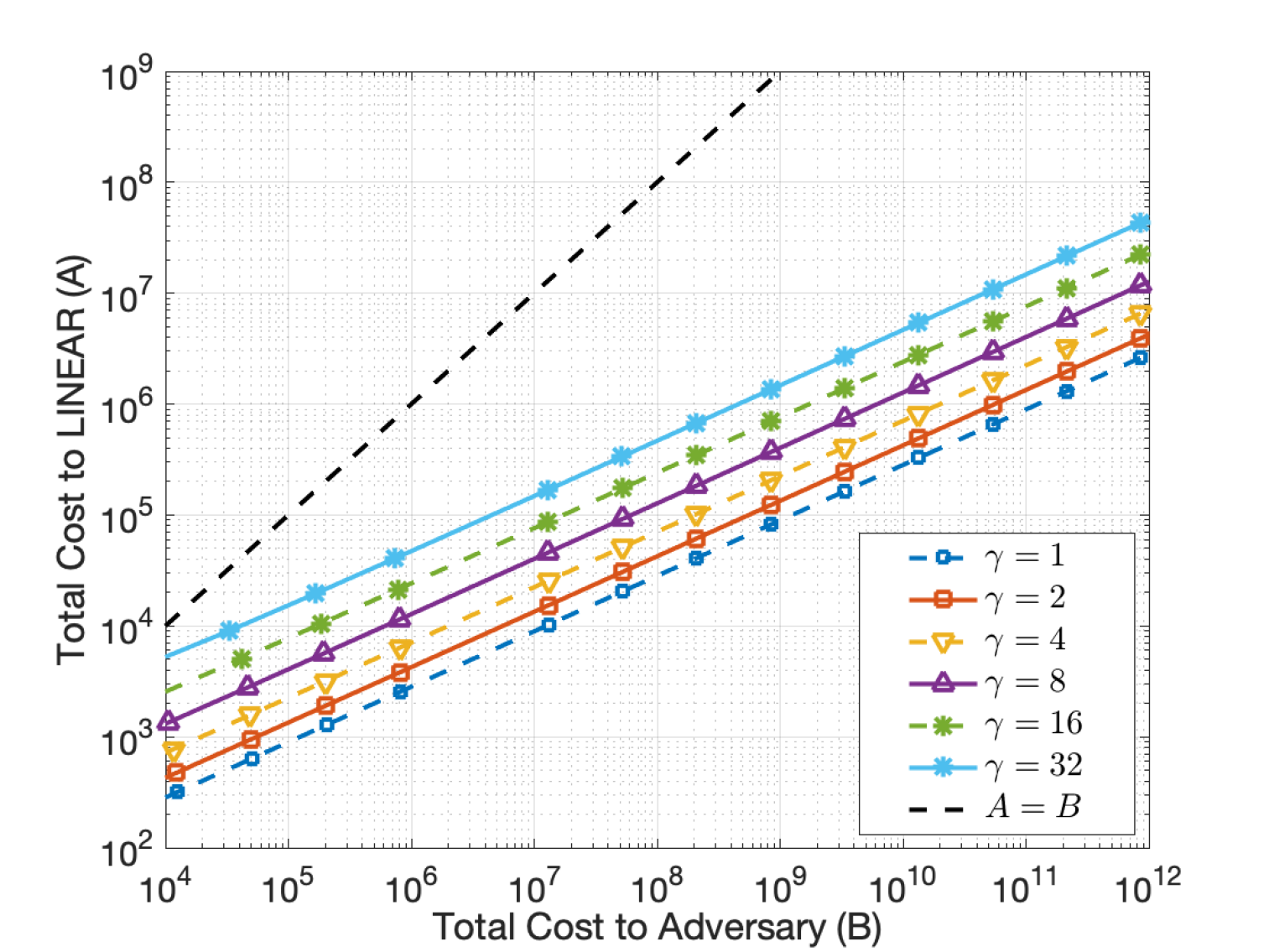
Figure 7: Results for LINEAR. (Left) $\gamma=1$; $\alpha$ value varies. (Right) $\alpha=1$; $\gamma$ value varies.

8.2 Experiments for LINEAR-POWER

To evaluate a challenging case for LINEAR-POWER, we create an input causing many bounced good jobs in the first iteration. From the start of this iteration, we consider disjoint periods of $2L$ seconds. Each period $i\geq 0$ will have $2^{i}$ bad jobs serviced, followed by $(i+1)M$ good jobs that are bounced. For example, in the first period, we have $1$ bad job serviced followed by $M$ good jobs; these $M$ good jobs will be bounced, since they start with a solution to a $1$-hard challenge, while the threshold has increased to $2$ due to the first bad job. In the second period, two bad jobs are serviced, followed by $M$ new good jobs, each starting with a $1$-hard RB solution. These are followed by the $M$ good jobs that were bounced in the first period. All of these $2M$ good jobs will be bounced, since the threshold has increased to $4$ due to the two bad jobs.

For each integer $z\in[10,28]$, we fix a number of bad jobs $b=2^{z}-1$, and let $M$ range over values $1,2,4,$ and $8$. Once all $b$ bad jobs have been serviced—which occurs in period $z$— a final batch of $M$ good jobs arrive with a $1$ hard solution and these are bounced. However, the other $(z+1)M$ (good) jobs will start being serviced. Specifically, $\gamma$ of these (good) jobs will be serviced, with the first $\gamma-1$ jobs (erroneously) considered bad by the estimator, and $\gamma$-th job (correctly) considered good; this ends the first iteration. All remaining good jobs will be serviced in subsequent iterations in similar fashion ($\gamma$ per iteration), since the threshold never again exceeds $2^{\left\lfloor\log(\gamma(\gamma+1))\right\rfloor}\leq\gamma(\gamma+1)$ (recall Lemma 2).

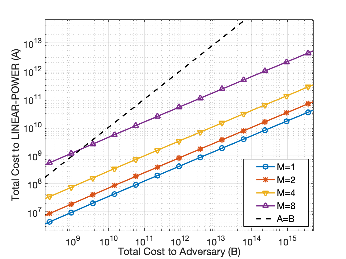
Figure 8: Our preliminary simulation results for LINEAR-POWER. Different values of $M$ are evaluated with $\gamma=8$.

Results for LINEAR-POWER. Figure 8 illustrates the results of our simulations when $\gamma=8$. As predicted by our upper bound on cost in Theorem 1.2, LINEAR-POWER achieves a lower cost than the adversary for $B$ sufficiently large. However, aligning with our analysis, we see that this cost advantage decreases as $M$ grows. In particular, between $M=1$ and $M=8$, we see the cost ratio decreases from roughly $2\times 10^{3}$ to $20$ for a fixed $B=9\times 10^{11}$. Very similar results are observed for other values of $\gamma$, and so we omit these and note that, for this set of experiments, the algorithm’s cost appears to be primarily sensitive to $M$.

9 Conclusion and Future Work

We have described and analyzed two deterministic algorithms for DoS defense. Our algorithms dynamically adjust the difficulty of RB challenges based on feedback from an estimator which estimates the number of good jobs in any time interval seen previously. The accuracy of the estimator on the input, the number and temporal placement of the good and bad jobs, and the Byzantine adversary’s cost are all unknown to the algorithm, but these all affect the algorithm’s cost.

Critically, during a significant attack the cost of our algorithm is asymptotically less than the cost to the adversary. We believe this is an important property for deterring economically-motivated DoS attacks. We have also described a lower bound for randomized algorithms showing that our algorithmic costs are asymptotically tight, whenever $\gamma$ is a constant. We note that, while our algorithms are deterministic, our lower bound holds even for randomized algorithms.

Finally, we gave simulation results to validate the performance predicted by our upper-bound results on the cost of our algorithms.

Future Work. We view our result as an encouraging step towards developing DoS defenses. However, many open problems remain.

First, can we handle heterogeneous jobs? In this paper, the provisioning cost to service any job is always $1$. Our results extend to the case where the provisioning cost for any two jobs does not differ by more than a constant factor. This captures settings where jobs are roughly homogeneous, or where the server terminates a job after a fixed amount of service is provided. However, an interesting next step is to address the case where the provisioning costs for jobs vary by more than a constant factor. The results of Scully, Grosof and Mitzenmacher[67] may be useful for addressing this problem.

Second, can we handle non-linear provisioning costs? In this paper, we consider a provisioning cost that scales linearly in the number of jobs. While this is a natural model, it may be interesting to consider different functions for the provisioning cost.

Third, can we model both the clients and the server as selfish but rational agents? In particular, can we design a mechanism that results in a Nash equilibrium, and also provides good cost performance as a function of the adversarial cost?

Fourth, can we get a more precise lower bound for our with-latency model? The lower bound in this paper holds in both models, but it is likely possible to get a better lower bound, in terms of the parameter $M$, for the with-latency model.

Finally, while our preliminary simulation results align with our upper bounds, a comprehensive evaluation may be valuable. This would be challenging, and would require significant effort to: (1) implement client and server processes; (2) determine an appropriate estimator, or create one for our specific purposes; and (3) generate network traffic that is faithful to real-world DDoS attacks.

References

- [1] Martin Abadi, Mike Burrows, Mark Manasse, and Ted Wobber. Moderately hard, memory-bound functions. ACM Transactions on Internet Technology (TOIT), 5(2):299–327, 2005.
- [2] M. Abliz and T. F. Znati. Defeating DDoS using productive puzzles. In 2015 International Conference on Information Systems Security and Privacy (ICISSP), pages 114–123, 2015.
- [3] Abhinav Aggarwal, Varsha Dani, Thomas Hayes, and Jared Saia. Secure One-Way Interactive Communication. In Proceedings of the 15th International Conference on Distributed Computing and Networking (ICDCN), 2017.
- [4] Isra Mohamed Ali, Maurantonio Caprolu, and Roberto Di Pietro. Foundations, properties, and security applications of puzzles: A survey. ACM Computing Survey, 53(4):1–38, 2020.
- [5] Tom Anderson, Timothy Roscoe, and David Wetherall. Preventing internet denial-of-service with capabilities. ACM SIGCOMM Computer Communication Review, 34(1):39–44, 2004.
- [6] Tuomas Aura, Pekka Nikander, and Jussipekka Leiwo. DoS-resistant authentication with client puzzles. In Proceedings of the International Workshop on Security Protocols, pages 170–177. Springer, 2000.
- [7] Rudolf Avenhaus, Bernhard Von Stengel, and Shmuel Zamir. Inspection games. Handbook of game theory with economic applications, 3:1947–1987, 2002.
- [8] AWS. AWS best practices for DDoS resiliency. https://docs.aws.amazon.com/whitepapers/latest/aws-best-practices-ddos-resiliency/aws-best-practices-ddos-resiliency.pdf, 2019.
- [9] Michael A. Bender, Jeremy T. Fineman, Seth Gilbert, and Maxwell Young. How to Scale Exponential Backoff: Constant Throughput, Polylog Access Attempts, and Robustness. In Proceedings of the Annual ACM-SIAM Symposium on Discrete Algorithms (SODA), pages 636–654, 2016.
- [10] Michael A. Bender, Jeremy T. Fineman, Mahnush Movahedi, Jared Saia, Varsha Dani, Seth Gilbert, Seth Pettie, and Maxwell Young. Resource-Competitive Algorithms. SIGACT News, 46(3):57–71, September 2015.
- [11] Michael A. Bender, Jeremy T. Fineman, Mahnush Movahedi, Jared Saia, Varsha Dani, Seth Gilbert, Seth Pettie, and Maxwell Young. Resource-competitive algorithms. SIGACT News, 46(3):57–71, September 2015.
- [12] Ken Binmore et al. Playing for real: a text on game theory. Oxford university press, 2007.
- [13] Nikita Borisov. Computational puzzles as Sybil defenses. In Proceedings of the IEEE International Conference on Peer-to-Peer Computing (P2P), pages 171–176, 2006.
- [14] Allan Borodin and Ran El-Yaniv. Online computation and competitive analysis. cambridge university press, 2005.
- [15] Glenn Carl, George Kesidis, Richard R Brooks, and Suresh Rai. Denial-of-service attack-detection techniques. IEEE Internet computing, 10(1):82–89, 2006.
- [16] Trisha Chakraborty. Simulation Code. https://github.com/trishac97/RB-Cost-DDOS, 2022.
- [17] Trisha Chakraborty, Shaswata Mitra, Sudip Mittal, and Maxwell Young. A policy driven ai-assisted pow framework. In 52nd Annual IEEE/IFIP International Conference on Dependable Systems and Networks, DSN 2022, Supplemental Volume, Baltimore, MD, USA, June 27-30, 2022, pages 37–38. IEEE, 2022.
- [18] Haimin Chen and Chaodong Zheng. Broadcasting competitively against adaptive adversary in multi-channel radio networks. In 24th International Conference on Principles of Distributed Systems, OPODIS, volume 184, pages 22:1–22:16, 2020.
- [19] Yu Chen, Wei-Shinn Ku, Kazuya Sakai, and Christopher DeCruze. A novel DDoS attack defending framework with minimized bilateral damages. In 2010 7th IEEE Consumer Communications and Networking Conference, pages 1–5. IEEE, 2010.
- [20] Fahad Zaman Chowdhury, Laiha Binti Mat Kiah, MA Manazir Ahsan, and Mohd Yamani Idna Bin Idris. Economic denial of sustainability (EDoS) mitigation approaches in cloud: Analysis and open challenges. In 2017 International Conference on Electrical Engineering and Computer Science (ICECOS), pages 206–211. IEEE, 2017.
- [21] Allen Clement, Harry Li, Jeff Napper, Jean-Philippe Martin, Lorenzo Alvisi, and Mike Dahlin. Bar primer. In 2008 IEEE International Conference on Dependable Systems and Networks With FTCS and DCC (DSN), pages 287–296. IEEE, 2008.
- [22] Allen Clement, Jeff Napper, Harry Li, Jean-Philipe Martin, Lorenzo Alvisi, and Michael Dahlin. Theory of bar games. In Proceedings of the twenty-sixth annual ACM symposium on Principles of distributed computing, pages 358–359, 2007.
- [23] Varsha Dani, Mahnush Movahedi, Jared Saia, and Maxwell Young. Interactive Communication with Unknown Noise Rate. In Proceedings of the Colloquium on Automata, Languages, and Programming (ICALP), 2015.
- [24] Roberto Doriguzzi-Corin, Stuart Millar, Sandra Scott-Hayward, Jesus Martinez-del Rincon, and Domenico Siracusa. LUCID: A practical, lightweight deep learning solution for DDoS attack detection. IEEE Transactions on Network and Service Management, 17(2):876–889, 2020.
- [25] Sever Silvestru Dragomir. Some refinements of jensen’s inequality. J. Math. Anal. Appl, 168(2):518–522, 1992.
- [26] Cynthia Dwork, Nancy Lynch, and Larry Stockmeyer. Consensus in the presence of partial synchrony. Journal of the ACM (JACM), 35(2):288–323, 1988.
- [27] Cynthia Dwork and Moni Naor. Pricing via processing or combatting junk mail. In Proceedings of the Annual International Cryptology Conference on Advances in Cryptology, pages 139–147, 1993.
- [28] Fei Fang, Thanh H Nguyen, Rob Pickles, Wai Y Lam, Gopalasamy R Clements, Bo An, Amandeep Singh, Brian C Schwedock, Milin Tambe, and Andrew Lemieux. Paws—a deployed game-theoretic application to combat poaching. AI Magazine, 38(1):23–36, 2017.
- [29] Fei Fang, Peter Stone, and Milind Tambe. When security games go green: Designing defender strategies to prevent poaching and illegal fishing. In IJCAI, pages 2589–2595, 2015.
- [30] Wu-chang Feng and Ed Kaiser. kapow webmail: Effective disincentives against spam. Proc. of 7th CEAS, 2010.
- [31] Seth Gilbert, Valerie King, Seth Pettie, Ely Porat, Jared Saia, and Maxwell Young. (Near) optimal resource-competitive broadcast with jamming. In Proceedings of the ACM Symposium on Parallelism in Algorithms and Architectures (SPAA), pages 257–266, 2014.
- [32] Seth Gilbert, Valerie King, Jared Saia, and Maxwell Young. Resource-competitive analysis: A new perspective on attack-resistant distributed computing. In Proceedings of the ACM International Workshop on Foundations of Mobile Computing, pages 1–6, 2012.
- [33] Seth Gilbert, Calvin Newport, Nitin H. Vaidya, and Alex Weaver. Contention resolution with predictions. In PODC ’21: ACM Symposium on Principles of Distributed Computing, Virtual Event, Italy, July 26-30, 2021, pages 127–137. ACM, 2021. doi:10.1145/3465084.3467911.
- [34] Seth Gilbert and Maxwell Young. Making Evildoers Pay: Resource-Competitive Broadcast in Sensor Networks. In Proceedings of the Symposium on Principles of Distributed Computing (PODC), pages 145–154, 2012.
- [35] Seth Gilbert and Chaodong Zheng. Sybilcast: Broadcast on the open airwaves. In Proceedings of the Annual ACM Symposium on Parallelism in Algorithms and Architectures (SPAA), pages 130–139, 2013.
- [36] Diksha Gupta, Jared Saia, and Maxwell Young. Proof of work without all the work. In Proceedings of the International Conference on Distributed Computing and Networking (ICDCN), 2018.
- [37] Diksha Gupta, Jared Saia, and Maxwell Young. Resource burning for permissionless systems. In International Colloquium on Structural Information and Communication Complexity, pages 19–44. Springer, 2020.
- [38] Diksha Gupta, Jared Saia, and Maxwell Young. Bankrupting Sybil despite churn. In Proceedings of the 41st IEEE International Conference on Distributed Computing Systems (ICDCS), 2021.
- [39] Jason D Hartline and Tim Roughgarden. Optimal mechanism design and money burning. In Proceedings of the Annual ACM Symposium on Theory of Computing, pages 75–84, 2008.
- [40] Steffen Huck and Wieland Müller. Burning money and (pseudo) first-mover advantages: an experimental study on forward induction. Games and Economic Behavior, 51(1):109–127, 2005.
- [41] Ari Juels and John Brainard. Client puzzles: A cryptographic countermeasure against connection depletion attacks. In Proceedings of the Network and Distributed System Security Symposium (NDSS), pages 151–165, 1999.
- [42] Ed Kaiser and Wu chang Feng. Mod_kaPoW: Mitigating DoS with transparent proof-of-work. In Proceedings of the ACM CoNEXT Conference, pages 74:1–74:2, 2007.
- [43] David Kempe, Leonard J Schulman, and Omer Tamuz. Quasi-regular sequences and optimal schedules for security games. In Proceedings of the Twenty-Ninth Annual ACM-SIAM Symposium on Discrete Algorithms, pages 1625–1644. SIAM, 2018.
- [44] Valerie King, Jared Saia, and Maxwell Young. Conflict on a Communication Channel. In Proceedings of the Symposium on Principles of Distributed Computing (PODC), pages 277–286, 2011.
- [45] Anusha Koduru, TulasiRam Neelakantam, and Mary Saira Bhanu S. Detection of economic denial of sustainability using time spent on a web page in cloud. In 2013 IEEE International Conference on Cloud Computing in Emerging Markets (CCEM), pages 1–4, 2013. doi:10.1109/CCEM.2013.6684433.
- [46] Oleg Kupreev, Ekaterina Badovskaya, and Alexander Gutnikov. DDoS attacks in Q1 2020. https://securelist.com/ddos-attacks-in-q1-2020/96837/, 2020.
- [47] Denise Berard (Kaspersky Labs). DDoS Breach Costs Rise to over $2M for Enterprises finds Kaspersky Lab Report. https://usa.kaspersky.com/about/press-releases/2018_ddos-breach-costs-rise-to-over-2m-for-enterprises-finds-kaspersky-lab-report, 2018.
- [48] Anukool Lakhina, Mark Crovella, and Christophe Diot. Diagnosing network-wide traffic anomalies. ACM SIGCOMM computer communication review, 34(4):219–230, 2004.
- [49] Silvio Lattanzi, Thomas Lavastida, Benjamin Moseley, and Sergei Vassilvitskii. Online scheduling via learned weights. In Proceedings of the Fourteenth Annual ACM-SIAM Symposium on Discrete Algorithms, pages 1859–1877. SIAM, 2020.
- [50] Frank Li, Prateek Mittal, Matthew Caesar, and Nikita Borisov. SybilControl: Practical Sybil defense with computational puzzles. In Proceedings of the Seventh ACM Workshop on Scalable Trusted Computing, pages 67–78, 2012.
- [51] Iuon-Chang Lin and Tzu-Chun Liao. A survey of blockchain security issues and challenges. IJ Network Security, 19(5):653–659, 2017.
- [52] Nancy A Lynch. Distributed algorithms. Elsevier, 1996.
- [53] Senthil Malliga, A Tamilarasi, and M Janani. Filtering spoofed traffic at source end for defending against DoS/DDoS attacks. In Proceedings of the International Conference on Computing, Communication and Networking, pages 1–5. IEEE, 2008.
- [54] David Mankins, Rajesh Krishnan, Ceilyn Boyd, John Zao, and Michael Frentz. Mitigating distributed denial of service attacks with dynamic resource pricing. In Proceedings of the Seventeenth Annual Computer Security Applications Conference, pages 411–421. IEEE, 2001.
- [55] Edward James McShane. Jensen’s inequality. Bulletin of the American Mathematical Society, 43(8):521–527, 1937.
- [56] Michael Mitzenmacher. A model for learned bloom filters, and optimizing by sandwiching. CoRR, abs/1901.00902, 2019. URL: http://arxiv.org/abs/1901.00902, arXiv:1901.00902.
- [57] Michael Mitzenmacher and Eli Upfal. Probability and Computing: Randomization and Probabilistic Techniques in Algorithms and Data Analysis. Cambridge University Press, 2017.
- [58] Michael Mitzenmacher and Sergei Vassilvitskii. Algorithms with Predictions. In Beyond the Worst-Case Analysis of Algorithms. T. Roughgarden, Ed. Cambridge University Press, 2021. doi:10.1017/9781108637435.
- [59] Michael Mitzenmacher and Sergei Vassilvitskii. Algorithms with predictions. Communications of the ACM, 65 (7):33–35, July 2022.
- [60] Jema David Ndibwile, A Govardhan, Kazuya Okada, and Youki Kadobayashi. Web server protection against application layer DDoS attacks using machine learning and traffic authentication. In Proceedings of the 39th IEEE Annual Computer Software and Applications Conference, pages 261–267, 2015.
- [61] Hukukane Nikaidô et al. On von neumann’s minimax theorem. Pacific J. Math, 4(1):65–72, 1954.
- [62] M. A. Noureddine, A. M. Fawaz, A. Hsu, C. Guldner, S. Vijay, T. Başar, and W. H. Sanders. Revisiting client puzzles for state exhaustion attacks resilience. In Proceedings of the Annual IEEE/IFIP International Conference on Dependable Systems and Networks (DSN), pages 617–629, 2019.
- [63] Georgios Oikonomou and Jelena Mirkovic. Modeling human behavior for defense against flash-crowd attacks. In Proceedings of the IEEE International Conference on Communications, pages 1–6. IEEE, 2009.
- [64] Bryan Parno, Dan Wendlandt, Elaine Shi, Adrian Perrig, Bruce Maggs, and Yih-Chun Hu. Portcullis: Protecting connection setup from denial-of-capability attacks. ACM SIGCOMM Computer Communication Review, 37(4):289–300, 2007.
- [65] Manish Purohit, Zoya Svitkina, and Ravi Kumar. Improving online algorithms via ML predictions. In Samy Bengio, Hanna M. Wallach, Hugo Larochelle, Kristen Grauman, Nicolò Cesa-Bianchi, and Roman Garnett, editors, Advances in Neural Information Processing Systems 31: Annual Conference on Neural Information Processing Systems 2018, NeurIPS 2018, December 3-8, 2018, Montréal, Canada, pages 9684–9693, 2018.
- [66] Arya Renjan, Karuna Pande Joshi, Sandeep Nair Narayanan, and Anupam Joshi. Dabr: Dynamic attribute-based reputation scoring for malicious IP address detection. In 2018 IEEE International Conference on Intelligence and Security Informatics (ISI), pages 64–69. IEEE, 2018.
- [67] Ziv Scully, Isaac Grosof, and Michael Mitzenmacher. Uniform bounds for scheduling with job size estimates. In Mark Braverman, editor, 13th Innovations in Theoretical Computer Science Conference, ITCS 2022, January 31 - February 3, 2022, Berkeley, CA, USA, volume 215 of LIPIcs, pages 114:1–114:30. Schloss Dagstuhl - Leibniz-Zentrum für Informatik, 2022. doi:10.4230/LIPIcs.ITCS.2022.114.
- [68] Ahmad Shawahna, Marwan Abu-Amara, Ashraf SH Mahmoud, and Yahya Osais. EDoS-ADS: An enhanced mitigation technique against economic denial of sustainability (EDoS) attacks. IEEE Transactions on Cloud Computing, 8(3):790–804, 2018.
- [69] Gaurav Somani, Manoj Singh Gaur, Dheeraj Sanghi, Mauro Conti, and Rajkumar Buyya. DDoS attacks in cloud computing: Issues, taxonomy, and future directions. Computer Communications, 107:30–48, 2017. doi:https://doi.org/10.1016/j.comcom.2017.03.010.
- [70] Milind Tambe. Security and game theory: algorithms, deployed systems, lessons learned. Cambridge university press, 2011.
- [71] Nighat Usman, Saeeda Usman, Fazlullah Khan, Mian Ahmad Jan, Ahthasham Sajid, Mamoun Alazab, and Paul Watters. Intelligent dynamic malware detection using machine learning in ip reputation for forensics data analytics. Future Generation Computer Systems, 118:124–141, 2021.
- [72] Luis Von Ahn, Manuel Blum, Nicholas J Hopper, and John Langford. CAPTCHA: Using hard AI problems for security. In Proceedings of the International Conference on the Theory and Applications of Cryptographic Techniques, pages 294–311. Springer, 2003.
- [73] Bernhard von Stengel. Recursive inspection games. Univ. der Bundeswehr München, Fak. für Informatik, 1991.
- [74] Michael Walfish, Mythili Vutukuru, Hari Balakrishnan, David Karger, and Scott Shenker. DDoS defense by offense. In Proceedings of the 2006 Conference on Applications, Technologies, Architectures, and Protocols for Computer Communications (SIGCOMM), pages 303–314, 2006.
- [75] Michael Walfish, Mythili Vutukuru, Hari Balakrishnan, David Karger, and Scott Shenker. DDoS defense by offense. ACM Transactions on Computer Systems (TOCS), 28(1):3, 2010.
- [76] XiaoFeng Wang and Michael K. Reiter. Defending against denial-of-service attacks with puzzle auctions. In Proceedings of the 2003 IEEE Symposium on Security and Privacy, pages 78–92, 2003.
- [77] Brent Waters, Ari Juels, Alex Halderman, and Edward Felten. New client puzzle outsourcing techniques for DoS resistance. In Proceedings of the 11th ACM Conference on Computer and Communications Security (CCS), pages 246–256, 2004.
- [78] Xiaowei Yang, David Wetherall, and Thomas Anderson. TVA: A DoS-limiting network architecture. IEEE/ACM Transactions on Networking, 16(6):1267–1280, 2008.
- [79] Andrew Yao. Probabilistic computations: Toward a unified measure of complexity. In Eighteenth IEEE Symposium on Foundations of Computer Science, pages 222–227, 1977.
- [80] Shui Yu, Theerasak Thapngam, Jianwen Liu, Su Wei, and Wanlei Zhou. Discriminating DDoS flows from flash crowds using information distance. In Proceedings of the Third International Conference on Network and System Security, pages 351–356. IEEE, 2009.
- [81] Shui Yu, Yonghong Tian, Song Guo, and Dapeng Oliver Wu. Can we beat DDoS attacks in clouds? IEEE Transactions on Parallel and Distributed Systems, 25(9):2245–2254, 2013.
- [82] Bin Yuan, Huan Zhao, Chen Lin, Deqing Zou, Laurence Tianruo Yang, Hai Jin, Ligang He, and Shui Yu. Minimizing financial cost of DDoS attack defense in clouds with fine-grained resource management. IEEE Transactions on Network Science and Engineering, 7(4):2541–2554, 2020.
- [83] Xiaoyong Yuan, Chuanhuang Li, and Xiaolin Li. DeepDefense: Identifying DDoS attack via deep learning. In Proceedings of the IEEE International Conference on Smart Computing (SMARTCOMP), pages 1–8, 2017.
- [84] Mahdi Zamani, Jared Saia, and Jedidiah Crandall. TorBricks: Blocking-Resistant Tor Bridge Distribution. In International Symposium on Stabilization, Safety, and Security of Distributed Systems (SSS), pages 426–440. Springer, 2017.
- [85] S. T. Zargar, J. Joshi, and D. Tipper. A survey of defense mechanisms against distributed denial of service (DDoS) flooding attacks. IEEE Communications Surveys Tutorials, 15(4):2046–2069, 2013.
- [86] Shengbao Zheng and Xiaowei Yang. Dynashield: Reducing the cost of DDoS defense using cloud services. In Proceedings of the 11th USENIX Workshop on Hot Topics in Cloud Computing (HotCloud 19), 2019.