Global existence of classical solutions and numerical simulations of a cancer invasion model

Abstract

In this paper, we study a cancer invasion model both theoretically and numerically. The model is a nonstationary, nonlinear system of three coupled partial differential equations modeling the motion of cancer cells, degradation of the extracellular matrix, and certain enzymes. We first establish existence of global classical solutions in both two- and three-dimensional bounded domains, despite the lack of diffusion of the matrix-degrading enzymes and corresponding regularizing effects in the analytical treatment. Next, we give a weak formulation and apply finite differences in time and a Galerkin finite element scheme for spatial discretization. The overall algorithm is based on a fixed-point iteration scheme. In order to substantiate our theory and numerical framework, several numerical simulations are carried out in two and three spatial dimensions.
Key words: haptotaxis, tumour invasion, global existence, fixed-point scheme, numerical simulations
AMS Classification (2020): 35A01, 35K57, 35Q92, 65M22, 65M60, 92C17

abstract=true

1 Introduction

The model.

One of the defining characteristics of a malignant tumour is its capability to invade adjacent tissues [20]; accordingly the mathematical literature directed at understanding underlying mechanisms is vast (see e.g. the surveys [28, 35]).

In this paper we focus on the following variant of a cancer invasion model developed by Perumpanani et al. [33] for the malignant invasion of tumours and investigate

$$\begin{cases}u_{t}=\frac{1}{\alpha}\Delta u-\chi\nabla\cdot(u\nabla c)+\mu u(1-u)&\text{in $\Omega\times(0,\infty)$},\\ c_{t}=-pc&\text{in $\Omega\times(0,\infty)$},\\ p_{t}=\frac{1}{\varepsilon}(uc-p)&\text{in $\Omega\times(0,\infty)$},\\ \frac{1}{\alpha}\partial_{\nu}u=\chi u\partial_{\nu}c&\text{on $\partial\Omega\times(0,\infty)$},\\ (u,c,p)(\cdot,0)=(u_{0},c_{0},p_{0})&\text{in $\Omega$}.\end{cases}$$ (1.1)

We aim for a rigorous existence proof for global solutions and the development of a reliable numerical scheme with an implementation in a modern open-source finite element library.

In (1.1), the motion of cancer cells (density denoted by $u$) mainly takes place by means of haptotaxis, i.e. directed motion toward higher concentrations of extracellular matrix (density $c$), of strength $χ\geq 0$. Motivated by experiments of Aznavoorian et al. [6], who reported only “a minor chemokinetic component” of the cell motion, the original model of [33] does not include a term for random (chemokinetic) cell motility at all. Acknowledging that “minor” does not mean “none at all”, we deviate from [33] in this aspect and incorporate this motility term in (1.1) ($α\in(0,\infty)$, with the formal limit $α\to∞$ corresponding to the model of [33]). Additional growth of the population of tumour cells is described by a logistic term (with $μ$ being a positive parameter). The extracellular matrix is degraded upon contact with certain enzymes (proteases, concentration $p$), which, in turn, are produced where cancer cells and matrix meet and decay over time. The reaction speed of these protein dynamics can be adjusted via the parameter $\varepsilon>0$. As many proteases remain bound to the cellular membrane – or are only activated when on the cell surface (cf. the model derivation in [33]), no diffusion for $p$ is incorporated in the model. This last point is in contrast to the otherwise similar popular models in the tradition of [3, 32] or [8], the latter of which additionally included a chemotactic component of the motion of cancer cells.

Global solvability.

In order to construct global classical solutions of (1.1), it is necessary to control the haptotaxis term $-\chi\nabla\cdot(u\nabla c)$ in the first equation and thus in particular to gain information on the spatial derivative of the second solution component. For relatives of (1.1) including a diffusion term $\Delta p$ in the third equation, this has already been achieved in [39] and [27] by applying parabolic regularity theory to the equation for $p$, first yielding estimates for the spatial derivative of $p$ and then also on $c$; the results of [27] even cover the long-term asymptotics of solutions. Moreover, the presence of diffusion for the produced quantities has also been made use of to obtain global existence results for different cancer invasion models, see for instance [41].

However, the absence of any spatial regularization in both the second and third equation makes the corresponding analysis much more challenging. Up to now, global classical solutions have only been constructed for a rather limited set of initial data: Already in [33], where (1.1) has been proposed for $\alpha=\infty$, it has been shown that the model formally obtained by taking the limit $\varepsilon\searrow 0$ admits a family of travelling wave solutions. Corresponding results for positive $\varepsilon$ have then been achieved in [30]. Moreover, if $\varepsilon=0$, travelling wave solutions may contain shocks [29] and solutions of related systems without a logistic source may even blow up in finite time [34]. In general, the destabilizing effect of taxis terms such as $-\chi\nabla\cdot(u\nabla c)$ may not only make it challenging but even impossible to obtain global existence results for certain problems. We refer to the survey [24] for further discussion regarding the consequences of low regularity in chemotaxis systems.

Despite these challenges, in the first part of the present paper we are able to give an affirmative answer to the question whether (1.1) also possesses global classical solutions for widely arbitrary initial data in the two and three-dimensional setting. Our analytical main result is the following

Theorem 1.1.

Suppose that $\alpha,\chi,\mu,\varepsilon$ are positive constants, that

$$\Omega\text{ is a smooth bounded domain in $\mathbb{R}^{n}$, $n\in\{1,2,3\}$,}$$

and that $u_{0},c_{0},p_{0}\in\bigcup_{\gamma\in(0,1)}C^{2+\gamma}(\overline{\Omega})$ are nonnegative and such that $\frac{1}{\alpha}\partial_{\nu}u_{0}=\chi u_{0}\partial_{\nu}c_{0}$ on $\partial\Omega$. Then there exists a unique global classical solution $(u,c,p)$ of (1.1) with regularity

$$(u,c,p)\in\big{(}C^{2,1}(\overline{\Omega}\times(0,\infty))\cap C^{1}(\overline{\Omega}\times[0,\infty))\big{)}^{3},$$

which, moreover, is nonnegative.

Numerical modeling.

In the second part of our paper we then analyze the behavior of these solutions numerically with an implementation in the modern open-source finite element library deal.II [5, 4]. Related numerical studies in various software libraries using different numerical schemes are briefly described in the following. The traditional method of lines has been widely used for simulations of the cancer invasion process [18, 14]. In addition, finite difference methods [22] have been considered and in [9, 21], the authors proposed a nonstandard finite difference method which satisfies the positivity-preservation of the solution, that is an important property in the stability of the model. Moreover, the finite volume method [10], spectral element methods [40], algebraically stabilized finite element method [36], the discontinuous Galerkin method [15], combinations of level-set/adaptive finite elements [43, 1], and a hybrid finite volume/finite element method [7, 2] have also been proposed in the literature for some cancer invasion models and chemotaxis. Finally, we mention that in [37] the authors illustrate their theoretical results for a related cancer model employing discontinuous Galerkin finite elements implemented as well in deal.II.

The main objective in the numerical part is the design of reliable algorithms for (1.1) and their corresponding implementation in deal.II. First, we discretize in time using a $\theta$-method, which allows for implicit $A$-stable time discretizations. Then, a Galerkin finite element scheme is employed for spatial discretization. The nonlinear discrete system of equations is decoupled by designing a fixed-point algorithm. This algorithm is newly designed and then implemented and debugged in deal.II.

These developments then allow to link our theoretical part and the numerical sections in order to carry out various numerical simulations to complement Theorem 1.1. Specifically, several parameter variations of the proliferation coefficient $\mu$ and the haptotactic coefficient $\chi$ will be studied in two- and three spatial dimensions. These studies are non-trivial due to the nonlinearities and the high sensitivity of (1.1) with respect to such parameter variations.

Plan of the paper.

The outline of this paper is as follows. In Section 2, we study the global existence of classical solutions. Next, in Section 3, we introduce the discretization in time and space using finite differences in time and a Galerkin finite element scheme in space. We also describe the solution algorithm. In Section 4, we carry out several numerical simulations demonstrating the properties of our model and the corresponding theoretical results. Therein, we specifically study parameter variations. Finally, our work is summarized in Section 5.

Notation.

Let $\Omega\subset\mathbb{R}^{n}$, $n\in\mathbb{N}$ be a bounded domain. By $L^{p}(\Omega)$ and $W^{1,p}(\Omega)$, we denote the usual Lebesgue and Sobolev spaces, respectively, and we abbreviate $H^{1}(\Omega)\coloneqq W^{1,2}(\Omega)$. Furthermore, $\langle\cdot,\cdot\rangle$ denotes the duality product between $(H^{1})^{*}$ and $H^{1}$.

For $m\in\mathbb{N}_{0}$ and $\gamma\in(0,1)$, we denote by $C^{m+\gamma}(\overline{\Omega})$ the space of functions $\varphi\in C^{m}(\overline{\Omega})$ with finite norm

$$\|\varphi\|_{C^{m+\gamma}(\overline{\Omega})}\coloneqq\|\varphi\|_{C^{m}(\overline{\Omega})}+\sup_{x,y\in\overline{\Omega},x\neq y}\frac{|\varphi(x)-\varphi(y)|}{|x-y|}.$$

Moreover, for $m_{1},m_{2}\in\mathbb{N}_{0}$, $\gamma_{1},\gamma_{2}\in[0,1)$ and $T>0$, we denote by $C^{m_{1}+\gamma_{1},m_{2}+\gamma_{2}}(\overline{\Omega}\times[0,T])$ the space of all functions $\varphi$ whose derivatives $D_{x}^{\alpha}D_{t}^{\beta}\varphi$, $|\alpha|\leq m_{1}$, $0\leq\beta\leq m_{2}$, (exist and) are continuous, and which have finite norm

$$\|\varphi\|_{C^{m_{1}+\gamma_{1},m_{2}+\gamma_{2}}(\overline{\Omega}\times[0,T])}\coloneqq\sum_{\begin{subarray}{c}|\alpha|\leq m_{1},\\ 0\leq\beta\leq m_{2}\end{subarray}}\|D_{x}^{\alpha}D_{t}^{\beta}\varphi\|_{C^{0}(\overline{\Omega}\times[0,T])}$$

$$+\sum_{\begin{subarray}{c}|\alpha|=m_{1},\\ 0\leq\beta\leq m_{2}\end{subarray}}\sup_{\begin{subarray}{c}x,y\in\overline{\Omega},x\neq y,\\ t\in[0,T]\end{subarray}}\frac{|D_{x}^{\alpha}D_{t}^{\beta}\varphi(x,t)-D_{x}^{\alpha}D_{t}^{\beta}\varphi(y,t)|}{|x-y|^{\gamma_{1}}}+\sum_{\begin{subarray}{c}|\alpha|\leq m_{1},\\ \beta=m_{2}\end{subarray}}\sup_{\begin{subarray}{c}x\in\overline{\Omega},\\ s,t\in[0,T],s\neq t\end{subarray}}\frac{|D_{x}^{\alpha}D_{t}^{\beta}\varphi(x,t)-D_{x}^{\alpha}D_{t}^{\beta}\varphi(x,s)|}{|t-s|^{\gamma_{2}}}.$$

Notationally, we do not distinguish between spaces of scalar- and vector-valued functions.

2 Global existence of classical solutions

As a first step in the proof of Theorem 1.1, we apply two transformations in Subsection 2.1; the first one allows us to get rid of some parameters in (1.1), the second one changes the first equation to a more convenient form. We then employ a fixed point argument to obtain a local existence result for the transformed system in Lemma 2.5.

The proof that these solutions are global in time consists of two key parts, both relying on the fact that the second and third equation in (1.1) at least regularize in time (which allows us to prove Lemma 2.7 and Lemma 2.10). First, in order to prove boundedness in $L^{\infty}$, the comparison principle allows us to conclude boundedness in small time intervals (cf. Lemma 2.8). We then iteratively apply this bound to obtain the result also for larger times (cf. Lemma 2.9). As to bounds for the spatial derivatives, we secondly apply a testing procedure to derive estimates valid on small time intervals (cf. Lemma 2.11), which then is again complemented by an iteration procedure (cf. Lemma 2.12). Finally, we are able to make use of parabolic regularity theory (inter alia in the form of maximal Sobolev regularity) to conclude in Lemma 2.14 that the solutions exist globally.

2.1 Two transformations

We first note that with regards to Theorem 1.1 we may without loss of generality assume $\chi=1$ and $\varepsilon=1$. Indeed, suppose that Theorem 1.1 holds for this special case. Then, assuming the conditions of Theorem 1.1 to hold, we set

$$\tilde{\alpha}\coloneqq\frac{\alpha\chi}{\varepsilon},\quad\tilde{\chi}\coloneqq 1,\quad\tilde{\mu}\coloneqq\varepsilon\mu,\quad\tilde{\varepsilon}\coloneqq 1$$

and further

$$\tilde{u}_{0}(\tilde{x})=u_{0}(\sqrt{\chi}\tilde{x}),\quad\tilde{c}_{0}(\tilde{x})=\varepsilon c_{0}(\sqrt{\chi}\tilde{x}),\quad\tilde{p}_{0}(\tilde{x})=\varepsilon p_{0}(\sqrt{\chi}\tilde{x})$$

for $\tilde{x}\in\tilde{\Omega}\coloneqq\frac{1}{\sqrt{\chi}}\Omega$. By Theorem 1.1, there then exists a global classical solution of (1.1) (with all parameters and initial data replaced by their pendants with tildes) $(\tilde{u},\tilde{c},\tilde{p})$. Then

$$(u,c,p)(x,t)\coloneqq\big{(}\tilde{u}(\tfrac{x}{\sqrt{\chi}},\tfrac{t}{\varepsilon}),\,\tfrac{1}{\varepsilon}\tilde{c}(\tfrac{x}{\sqrt{\chi}},\tfrac{t}{\varepsilon}),\,\tfrac{1}{\varepsilon}\tilde{p}(\tfrac{x}{\sqrt{\chi}},\tfrac{t}{\varepsilon})\big{)},\quad(x,t)\in(\overline{\Omega}\times[0,\infty)),$$ (2.1)

fulfills

$$\begin{cases}u_{t}=\frac{\chi}{\tilde{\alpha}\varepsilon}\Delta u-\frac{\varepsilon\chi}{\varepsilon}\nabla\cdot(u\nabla c)+\frac{\tilde{\mu}}{\varepsilon}u(1-u)&\text{in $\Omega\times(0,\infty)$},\\[1.99997pt] c_{t}=-\frac{\varepsilon^{2}}{\varepsilon^{2}}cp&\text{in $\Omega\times(0,\infty)$},\\[1.99997pt] p_{t}=\frac{1}{\varepsilon^{2}}(\varepsilon uc-\varepsilon p)&\text{in $\Omega\times(0,\infty)$},\\[1.99997pt] \partial_{\nu}u=\frac{\tilde{\alpha}\varepsilon\sqrt{\chi}}{\sqrt{\chi}}u\partial_{\nu}c&\text{on $\partial\Omega\times(0,\infty)$},\\[1.99997pt] (u,c,p)(x,0)=(\tilde{u}_{0},\frac{1}{\varepsilon}\tilde{c}_{0},\frac{1}{\varepsilon}\tilde{p}_{0})(\frac{x}{\sqrt{\chi}})&\text{for $x\in\Omega$}\end{cases}$$

and thus (1.1). Moreover, following precedents from, e.g. [12, p.19], we set

$$w(x,t)\coloneqq u(x,t)\mathrm{e}^{-αc(x,t)},\qquad x\in\overline{\Omega},\;t\geq 0.$$ (2.2)

Then $∇w=\mathrm{e}^{-αc}∇u-α\mathrm{e}^{-αc}u∇c$, so that

$$\tfrac{1}{\alpha}\Delta w+\nabla c\cdot\nabla w=\mathrm{e}^{-\alpha c}∇\cdot(\tfrac{1}{α}\mathrm{e}^{αc}∇w)=\mathrm{e}^{-\alpha c}[\tfrac{1}{α}Δu-∇\cdot(u∇c)]$$ (2.3)

and (1.1) (with $\chi=\varepsilon=1$) is equivalent to

$$\begin{cases}w_{t}=\frac{1}{\alpha}\Delta w+\nabla c\cdot\nabla w+αpcw+μw-μ\mathrm{e}^{αc}w^{2}&\text{in $\Omega\times(0,\infty)$},\\ c_{t}=-pc&\text{in $\Omega\times(0,\infty)$},\\ p_{t}=w\mathrm{e}^{αc}c-p&\text{in $\Omega\times(0,\infty)$},\\ \partial_{\nu}w=0&\text{on $\partial\Omega\times(0,\infty)$},\\ (w,c,p)(\cdot,0)=(w_{0},c_{0},p_{0})&\text{in $\Omega$}\end{cases}$$ (2.4)

for $w_{0}\coloneqq u_{0}\mathrm{e}^{-αc_{0}}$. Expanding $\nabla\cdot(u\nabla c)$ to $\nabla u\cdot\nabla c+u\Delta c$ shows that this transformation allows us to get rid of a term involving $\Delta c$ in the first equation at the price of adding several zeroth order terms. In particular as the second equation does not regularize in space, (2.4) turns out to be a more convenient form for the following analysis.

2.2 Local existence

In this subsection, we construct maximal classical solutions of (2.4) in $\overline{\Omega}\times[0,T_{\max})$ for some $T_{\max}\in[0,\infty)$ by means of a fixed point argument. Moreover, we provide a criterion for when these solutions are global in time (that is, when $T_{\max}=\infty$ holds), which then will finally be seen to hold true in Lemma 2.14.

As a preparation, we first collect results on (Hölder) continuous dependency of solutions to ODEs on the data.

Lemma 2.1.

Let $\Omega\subset\mathbb{R}^{n}$, $n\in\mathbb{N}$, be a bounded domain, $T>0$, $d\in ℕ$, $γ_{1},γ_{2}\in[0,1)$, $v_{0}\in C^{γ_{1}}(\overline{\Omega})$ and assume that $f\colon\overline{\Omega}\times[0,T]\times ℝ^{d}\to ℝ^{d}$ is $(γ_{1},γ_{2})$-Hölder continuous with respect to its first two arguments and locally Lipschitz continuous w.r.t. the third variable, in the sense that for every compact $K\subset ℝ^{d}$ there is $L>0$ such that

$$\sup_{t\in[0,T],v\in K}\|f(\cdot,t,v)\|_{C^{γ_{1}}(\overline{\Omega})} \leq L,$$

$$\sup_{x\in\overline{\Omega},v\in K}\|f(x,\cdot,v)\|_{C^{γ_{2}}([0,T])} \leq L,$$

$$\sup_{(x,t)\in\overline{\Omega}\times[0,T]}|f(x,t,v)-f(x,t,w)| \leq L|v-w|\quad\text{for all }v,w\in K.$$

Then for any compact $K\subset ℝ^{d}$ there is $C>0$ such that whenever $v\colon\overline{\Omega}\times[0,T]\to\mathbb{R}^{d}$ is such that $v(x,\cdot)\in C^{0}([0,T])\cap C^{1}((0,T))$ for all $x\in\overline{\Omega}$, $v$ solves

$$v_{t}(x,t)=f(x,t,v(x,t))\quad\text{ for all }x\in\overline{\Omega},t\in(0,T);\qquad v(x,0)=v_{0}(x)\quad\text{for all }x\in\overline{\Omega}$$ (2.5)

and satisfies $v(\overline{\Omega}\times[0,T])\subset K$, then $v,v_{t}\in C^{γ_{1},γ_{2}}(\overline{\Omega}\times[0,T])$ and

$$\|v\|_{C^{γ_{1},1+γ_{2}}(\overline{\Omega}\times[0,T])}\leq C.$$

• First, we let $K$ be a compact superset of $v(\overline{\Omega}\times[0,T])$ and let $L$ be as in the assumptions on $f$. We introduce $ω_{1}\in C^{0}([0,∞))$ such that $|f(x,t,w)-f(y,t,w)|\leq ω_{1}(|x-y|)$ for all $x\in\overline{\Omega}$, $y\in\overline{\Omega}$, $t\in[0,T]$ and $w\in K$, $|v_{0}(x)-v_{0}(y)|\leq ω_{1}(|x-y|)$ for all $x\in\overline{\Omega}$, $y\in\overline{\Omega}$ and such that $ω_{1}(0)=0$ and $\sup_{r>0}r^{-γ_{1}}ω_{1}(r)<∞$. We then fix $x\in\overline{\Omega}$, $y\in\overline{\Omega}\setminus\left\{x\right\}$ and let $\tilde{v}(t)=(v(x,t)-v(y,t))\cdot\frac{1}{ω_{1}(|x-y|)}$. Then

  $$\tilde{v}_{t}(t) =\frac{1}{ω_{1}(|x-y|)}(f(x,t,v(x,t))-f(y,t,v(x,t))+\frac{1}{ω_{1}(|x-y|)}(f(y,t,v(x,t))-f(y,t,v(y,t)))$$

  $$\leq 1+\frac{L}{ω_{1}(|x-y|)}|v(x,t)-v(y,t)|\qquad\text{for all $t\in(0,T)$},$$

  so that $\tilde{v}_{t}\leq 1+L|\tilde{v}|$ and, analogously, $\tilde{v}_{t}\geq-1-L|\tilde{v}|$, so that boundedness of $|\tilde{v}|$ results from Grönwall’s inequality and hence $v\in C^{\gamma_{1},0}(\overline{\Omega}\times[0,T])$, and $\sup_{t\in[0,T]}\|v(\cdot,t)\|_{C^{γ_{1}}(\overline{\Omega})}$ is bounded due to the choice of $\omega_{1}$.

  For $τ>0$, we treat $\bar{v}(x,t)=(v(x,t)-v(x,t+τ))/ω_{2}(τ)$ with some $ω_{2}$ such that $|f(x,t,v)-f(x,t+τ,v)|\leq ω_{2}(τ)$ in the same way. This ensures the claimed regularity of $v$, whereupon that of $v_{t}$ follows from $v_{t}(x,t)=f(x,t,v(x,t))$, $(x,t)\in\overline{\Omega}\times(0,T)$ and continuity of the right-hand side up to $t=0$ and $t=T$. ∎

Lemma 2.2.

In addition to the assumptions of Lemma 2.1, let $m\in\mathbb{N}$ and $v_{0}\in C^{m+γ_{1}}(\overline{\Omega})$. If all derivatives of $f$ w.r.t. $x$ and $v$ up to order $m$ satisfy the conditions Lemma 2.1 poses on $f$, then any solution $v$ as in Lemma 2.1 belongs to $C^{m+γ_{1},1+γ_{2}}(\overline{\Omega}\times[0,T])$.

• For $i\in\left\{1,\ldots,n\right\}$, $\tilde{v}=∂_{x_{i}}v$ satisfies

  $$\tilde{v}_{t}=f_{x_{i}}(x,t,v(x,t))+f_{v}(x,t,v(x,t))\tilde{v}\quad\text{in }\Omega\times(0,T),\qquad\tilde{v}(\cdot,0)=(v_{0})_{x_{i}}\text{ in }\Omega$$

  and Lemma 2.1 can be applied to $\tilde{v}$. An inductive argument takes care of higher derivatives. ∎

By applying these results to the ODEs appearing in (2.4), we obtain

Lemma 2.3.

Let $\Omega\subset ℝ^{n}$, $n\in\mathbb{N}$, be a bounded domain, $α\geq 0$ and $T\in(0,\infty)$. Let $0\leq w\in C^{0}(\overline{\Omega}\times[0,T])$ and $c_{0},p_{0}\in C^{0}(\overline{\Omega};[0,\infty))$.
a) Then

$$\begin{cases}c_{t}=-pc\\ p_{t}=w\mathrm{e}^{αc}c-p\end{cases}$$ (2.6)

has a unique solution $(c,p)\in(C^{0,1}(\overline{\Omega}\times[0,T]))^{2}$.
b) For any $M>0$ there is $C=C(M)>0$ such that whenever $\tilde{T}\in(0,T]$, $w\in C^{1,0}(\overline{\Omega}\times[0,\tilde{T}])$, $c_{0},p_{0}\in C^{1}(\overline{\Omega})$ with

$$\sup_{t\in[0,\tilde{T}]}\|w(\cdot,t)\|_{C^{1}(\overline{\Omega})}\leq M,\quad\|c_{0}\|_{C^{1}(\overline{\Omega})}\leq M,\quad\|p_{0}\|_{C^{1}(\overline{\Omega})}\leq M,$$

then

$$\|(c,p)\|_{C^{1}(\overline{\Omega}\times[0,\tilde{T}])}\leq C.$$

c) If, for some $k\in ℕ_{0}$ and $γ_{1},γ_{2}\in[0,1)$, $w\in C^{k+γ_{1},γ_{2}}(\overline{\Omega}\times[0,T])$ and $c_{0},p_{0}\in C^{k+γ_{1}}(\overline{\Omega})$, then $c,p\in C^{k+γ_{1},1+γ_{2}}(\overline{\Omega}\times[0,T])$.

• a) Given $w\in C^{0}(\overline{\Omega}\times[0,T])$, for every $x\in\overline{\Omega}$ the existence and uniqueness of a solution $(c,p)(x,\cdot)\in C^{0}([0,T_{\max}(x)])\cap C^{1}((0,T_{\max}(x)))$ of (2.6), with some $T_{\max}(x)\in(0,T]$ such that $\limsup_{t\nearrow T_{\max}(x)}(|c(x,t)|+|p(x,t)|)=\infty$ or $T_{\max}(x)=T$, follows from Picard–Lindelöf’s theorem. By an ODE comparison argument, nonnegativity of $c$ follows from that of $c_{0}$, and nonnegativity of $p$ from that of $p_{0}$, $w$ and $c$. Therefore, $0\leq c(x,t)\leq c_{0}(x)$ for all $x\in\overline{\Omega}$ and $t\in(0,T_{\max}(x))$ due to the sign of $c_{t}=-pc$. Consequently,

  $$p(x,t) =\mathrm{e}^{-t}p_{0}(x)+\int_{0}^{t}\mathrm{e}^{-(t-s)}w(x,s)\mathrm{e}^{αc(x,s)}c(x,s)\,\mathrm{d}s$$

  $$\leq\max\left\{p_{0}(x),c_{0}(x)\mathrm{e}^{αc_{0}(x)}\max_{s\in[0,T]}w(x,s)\right\}\qquad\text{for all }x\in\overline{\Omega},t\in[0,T_{\max}(x)),$$

  which also shows that $T_{\max}(x)=T$ for all $x\in\overline{\Omega}$. The remainder of part a) follows from an application of Lemma 2.1 with $γ_{1}=γ_{2}=0$.
  b) We apply Lemma 2.1 to $v=(∇c,∇p)$, the solution of

  $$v_{t}=\begin{pmatrix}-pI_{n\times n}&-cI_{n\times n}\\ (αw\mathrm{e}^{αc}c+w\mathrm{e}^{αc})I_{n\times n}&-I_{n\times n}\end{pmatrix}v+\begin{pmatrix}0\\ \mathrm{e}^{αc}c∇w\end{pmatrix},\qquad v(0)=\begin{pmatrix}\nabla c_{0}\\ \nabla p_{0}\end{pmatrix}\in\mathbb{R}^{2n},$$

  noting that sufficient regularity is given by the assumption on $w$ and part a).
  c) follows from Lemma 2.2. ∎

Both as an ingredient to the proof of Lemma 2.5 below and also for its own interest, we note that classical solutions of (2.4) are unique.

Lemma 2.4.

Let $\Omega\subset\mathbb{R}^{n}$, $n\in\mathbb{N}$, a bounded domain and let $\alpha,\mu>0$ as well as $\chi=\varepsilon=1$. Suppose $(u_{1},c_{1},p_{1})$ and $(u_{2},c_{2},p_{2})$ are two solutions of (1.1) with the same initial data $(u_{0},c_{0},p_{0})\in C^{0}(\overline{\Omega})\times C^{1}(\overline{\Omega})\times C^{1}(\overline{\Omega})$ and assume that they belong to

$$\left(C^{2,1}(\overline{\Omega}\times(0,T))\cap C^{1}(\overline{\Omega}\times[0,T])\right)^{3}$$

for some $T>0$. Then $(u_{1},c_{1},p_{1})=(u_{2},c_{2},p_{2})$ in $\overline{\Omega}\times[0,T]$.

• We let $C>0$ be such that

  $$\max\left\{\|u_{i}(\cdot,t)\|_{L^{\infty}(\Omega)},\|∇u_{i}(\cdot,t)\|_{L^{\infty}(\Omega)},\|c_{i}(\cdot,t)\|_{L^{\infty}(\Omega)},\|p_{i}(\cdot,t)\|_{L^{\infty}(\Omega)},\|∇c_{i}(\cdot,t)\|_{L^{\infty}(\Omega)},\|∇p_{i}(\cdot,t)\|_{L^{\infty}(\Omega)}\right\}\leq C$$

  for all $t\in[0,T]$ and $i\in\left\{1,2\right\}$. Then computing

  $$\frac{1}{2} \frac{\mathrm{d}}{\mathrm{d}t}\left(\int_{\Omega}(u_{1}-u_{2})^{2}+\int_{\Omega}(c_{1}-c_{2})^{2}+\int_{\Omega}(p_{1}-p_{2})^{2}+\int_{\Omega}|∇(c_{1}-c_{2})|^{2}+\int_{\Omega}|∇(p_{1}-p_{2})|^{2}\right)$$

  $$=-\frac{1}{α}\int_{\Omega}|∇(u_{1}-u_{2})|^{2}+\int_{\Omega}∇(u_{1}-u_{2})[(u_{1}-u_{2})∇c_{1}+u_{2}∇(c_{1}-c_{2})]+μ\int_{\Omega}(u_{1}-u_{2})^{2}$$

  $$\quad-μ\int_{\Omega}(u_{1}-u_{2})^{2}(u_{1}+u_{2})-\int_{\Omega}(c_{1}-c_{2})(p_{1}-p_{2})c_{1}-\int_{\Omega}(c_{1}-c_{2})^{2}p_{2}-\int_{\Omega}(p_{1}-p_{2})^{2}$$

  $$\quad+\int_{\Omega}(p_{1}-p_{2})u_{1}(c_{1}-c_{2})+\int_{\Omega}(p_{1}-p_{2})(u_{1}-u_{2})c_{2}-\int_{\Omega}∇(c_{1}-c_{2})∇(p_{1}-p_{2})c_{1}$$

  $$\quad-\int_{\Omega}∇(c_{1}-c_{2})(p_{1}-p_{2})∇c_{1}-\int_{\Omega}p_{2}|∇(c_{1}-c_{2})|^{2}-\int_{\Omega}∇(c_{1}-c_{2})(c_{1}-c_{2})∇p_{2}$$

  $$\quad-\int_{\Omega}|∇(p_{1}-p_{2})|^{2}+\int_{\Omega}∇(p_{1}-p_{2})(c_{1}-c_{2})∇u_{1}+\int_{\Omega}∇(p_{1}-p_{2})u_{1}∇(c_{1}-c_{2})$$

  $$\quad+\int_{\Omega}∇(p_{1}-p_{2})∇(u_{1}-u_{2})c_{2}+\int_{\Omega}∇(p_{1}-p_{2})(u_{1}-u_{2})∇c_{2}$$

  $$\leq((2+αC)C+μ+2Cμ)\int_{\Omega}(u_{1}-u_{2})^{2}+5C\int_{\Omega}(c_{1}-c_{2})^{2}+(4C-1)\int_{\Omega}(p_{1}-p_{2})^{2}$$

  $$\quad+(5+αC)C\int_{\Omega}|∇(c_{1}-c_{2})|^{2}+((4+αC)C-1)\int_{\Omega}|∇(p_{1}-p_{2})|^{2}\qquad\text{in }(0,T),$$

  we obtain $(u_{1},c_{1},p_{1})=(u_{2},c_{2},p_{2})$ from Grönwall’s inequality. ∎

Making use of Schauder’s fixed point theorem and applying Lemmata 2.1–2.4, we now obtain a local existence result for the system (2.4).

Lemma 2.5.

Assume that

$$\Omega\text{ is a smooth bounded domain in $\mathbb{R}^{n}$, $n\in\{1,2,3\}$, }\alpha,\mu>0$$ (2.7)

and that

$$w_{0},c_{0},p_{0}\in C^{2+\gamma}(\overline{\Omega})\quad\text{for some $\gamma\in(0,1)$ are nonnegative and fulfill}\quad\partial_{\nu}w_{0}=0\text{ on $\partial\Omega$}.$$ (2.8)

Then (2.4) has a nonnegative unique solution

$$(w,c,p)\in\left(C^{2+\gamma,1+\frac{\gamma}{2}}(\overline{\Omega}\times(0,T_{\max}))\cap C^{1}(\overline{\Omega}\times[0,T_{\max}))\right)^{3}$$

for some $T_{\max}>0$, which can be chosen such that

$$T_{\max}=\infty\quad\text{ or }\quad\limsup_{t\nearrow T_{\max}}\|w(\cdot,t)\|_{C^{1+γ}(\overline{\Omega})}=\infty$$ (2.9)

• For $T>0$ and $M>0$ we introduce the set

  $$S_{M,T}=\left\{w\in C^{0}([0,T];C^{1}(\overline{\Omega}))\mid 0\leq w,\sup_{t\in[0,T]}\|w(\cdot,t)\|_{C^{1}(\overline{\Omega})}\leq M\right\}$$

  and given $w\in S_{M,T}$ we let $(c,p)$ be the solution of (2.6) (cf. Lemma 2.3 a)). We then let $v$ be the unique (weak) solution (see [23, Theorem III.5.1], [26, Theorem 6.39]) of

  $$v_{t}=\frac{1}{α}Δv+f\cdot∇v+gv\text{ in }\Omega\times(0,T),\qquad∂_{ν}v=0\text{ on }∂\Omega\times(0,T),\qquad v(\cdot,0)=w_{0}\text{ in }\Omega,$$ (2.10)

  where $f=∇c$ and $g=αpc+μ-μ\mathrm{e}^{αc}w$ belong to $L^{\infty}(\Omega\times(0,T))$ according to Lemma 2.3 a) and b), and define $Φ(w)=v$ in $\overline{\Omega}\times[0,T]$.

  We choose $M>0$ such that

  $$M>\|c_{0}\|_{C^{1}(\overline{\Omega})},\quad M>\|p_{0}\|_{C^{1}(\overline{\Omega})},\quad M>\|w_{0}\|_{C^{1+γ}(\overline{\Omega})},\qquad M>\|w_{0}\|_{C^{1}(\overline{\Omega})}+1$$ (2.11)

  and introduce the constants $c_{1}=c_{1}(M)$ from Lemma 2.3 b) (for $T=1$), $c_{2}>0$ from [26, Theorem 6.40] such that all solutions $v$ of (2.10) with $\|f\|_{L^{\infty}(\Omega\times(0,T))}\leq c_{1}$, $\|g\|_{L^{\infty}(\Omega\times(0,T))}\leq αc_{1}^{2}+μ+μ\mathrm{e}^{αc_{1}}M$ and $\|w_{0}\|_{L^{\infty}(\Omega)}\leq M$ satisfy $\|v\|_{L^{\infty}(\Omega\times(0,T))}\leq c_{2}$, and $c_{3}>0$ such that by [25, Theorems 1.1 and 1.2], all solutions $v$ of (2.10) with $∂_{ν}w_{0}=0$ on $∂\Omega$, $\|w_{0}\|_{C^{1+γ}(\overline{\Omega})}\leq M$, $\|f\|_{L^{\infty}(\Omega\times(0,T))}\leq c_{1}$, $\|g\|_{L^{\infty}(\Omega\times(0,T))}\leq αc_{1}^{2}+μ\mathrm{e}^{αc_{1}}+μ\mathrm{e}^{2αc_{1}}M$ and $\|v\|_{L^{\infty}(\Omega\times(0,T))}\leq c_{2}$ also fulfil $\|v\|_{C^{1+γ,\frac{1+γ}{2}}(\overline{\Omega}\times[0,T])}\leq c_{3}$. Finally, we fix $T\in(0,1]$ such that $c_{3}\sqrt{T}\leq 1$.

  Successive applications of Lemma 2.3, [26, Theorem 6.40] and [25, Theorems 1.1 and 1.2] then ensure that

  $$\|Φ(w)\|_{C^{1+γ,\frac{γ}{2}}(\overline{\Omega}\times[0,T])}\leq c_{3}.$$ (2.12)

  In particular,

  $$\|Φ(w)(\cdot,t)\|_{C^{1}(\overline{\Omega})}\leq\|Φ(w)(\cdot,0)\|_{C^{1}(\overline{\Omega})}+\|Φ(w)(\cdot,t)-Φ(w)(\cdot,0)\|_{C^{1}(\overline{\Omega})}\leq\|w_{0}\|_{C^{1}(\overline{\Omega})}+c_{3}t^{\frac{1}{2}}\leq M$$

  for every $t\in[0,T]$. Apparently, $\Phi$ maps $S_{M,T}$ to itself and, according to (2.12) has a compact image. Schauder’s fixed point theorem provides a fixed point $w$ of $\Phi$, that is, (together with $c$ and $p$) a solution of (2.4) in $\Omega\times[0,T]$.

  As $w\in C^{1+γ,0}(\overline{\Omega}\times[0,T_{\max}))$, $p,c,∇c$ belong to $C^{γ,\frac{γ}{2}}(\overline{\Omega}\times[0,T_{\max}))$ by Lemma 2.3 c) with $γ_{2}=0$. Since moreover $w\in C^{\gamma,\frac{\gamma}{2}}(\overline{\Omega}\times[0,T_{\max}))$, also $f$ and $g$ in (2.10) belong to this space. Then [23, Theorem IV.5.3] (if combined with the uniqueness statement of [23, Theorem III.5.1] and $C^{2+γ}$ regularity of $w_{0}$) makes $w$ a classical solution with $w_{t},D_{x}^{2}w\in C^{\gamma,\frac{\gamma}{2}}(\overline{\Omega}\times[0,T_{\max}))$. An invocation of Lemma 2.3 c) yields $D_{x}^{2}c,D_{x}^{2}p,\nabla p\in C^{\gamma,1+\frac{\gamma}{2}}(\overline{\Omega}\times[0,T_{\max}))$. Another application of [23, Theorem IV.5.3] to $\zeta w$ for a temporal cuttoff function $\zeta$ ensures that $\nabla w_{t}\in C^{\gamma,\frac{\gamma}{2}}(\overline{\Omega}\times(0,T_{\max}))$. Moreover, nonnegativity of $w$ as well as of $c$ and $p$ follows from the comparison principles for parabolic and ordinary differential equations, respectively.

  Since $M$ and $T$ only depend on the quantities in (2.11) and as solutions are unique by Lemma 2.4; the above reasoning can therefore be applied to extend the solution until some maximal existence time characterized by

  $$T_{\max}=\infty\quad\text{ or }\quad\limsup_{t\nearrow T_{\max}}\left(\|c(\cdot,t)\|_{C^{1}(\overline{\Omega})}+\|p(\cdot,t)\|_{C^{1}(\overline{\Omega})}+\|w(\cdot,t)\|_{C^{1+γ}(\overline{\Omega})}\right)=\infty.$$ (2.13)

  According to Lemma 2.3 b), boundedness of the norm of $w$ in this expression already implies that of the norms of $c$ and $p$, therefore (2.13) can be reduced to (2.9).

  Finally, uniqueness of this solution has already been asserted in Lemma 2.4. ∎

By fixing initial data as in (2.8), we henceforth implicitly also fix the unique classical solution $(w,c,p)$ of (2.4) given by Lemma 2.5 and denote its maximal existence time by $T_{\max}$.

2.3 $L^{\infty}$ bounds

The results in the previous subsection show that Theorem 1.1 follows once we have shown that for the solutions constructed in Lemma 2.5 the second alternative in (2.9) holds. That is, we need to derive sufficiently strong a priori estimates. In this subsection, we begin with bounds in $L^{\infty}$.

For the second solution component, such a bound directly follows from the comparison principle.

Lemma 2.6.

Suppose (2.7) and that $(w_{0},c_{0},p_{0})$ satisfies (2.8). Then the solution $(w,c,p)$ constructed in Lemma 2.5 fulfills

$$\|c(\cdot,t)\|_{L^{\infty}(\Omega)}\leq\|c_{0}\|_{L^{\infty}(\Omega)}\qquad\text{for all $t\in(0,T_{\max})$}.$$

• The function $\overline{c}\coloneqq\|c_{0}\|_{L^{\infty}(\Omega)}$ is a supersolution of the second equation in (2.4) and $c\geq 0$ by Lemma 2.5. ∎

As a preparation for obtaining $L^{\infty}$ estimates also for the other two solution components, we note that the time regularization in the third equation in (2.4) implies that we can bound $p$ by a quantity including an arbitrarily small contribution of the $L^{\infty}$ norm of $w$ – at least if we are willing to shrink the time interval on which this estimates holds accordingly.

Lemma 2.7.

Suppose (2.7) and let $M>0$. Then there exists $T^{\star}>0$ such that for all $(w_{0},c_{0},p_{0})$ satisfying (2.8) and

$$\|c_{0}\|_{L^{\infty}(\Omega)}\leq M,$$

the solution $(w,c,p)$ of (2.4) fulfills

$$\|p\|_{L^{\infty}(\Omega\times(0,T))}\leq\|p_{0}\|_{L^{\infty}(\Omega)}+\min\left\{\frac{\mu}{2M\alpha},1\right\}\|w\|_{L^{\infty}(\Omega\times(0,T))}\qquad\text{for all $T\in(0,T^{\star}]\cap(0,T_{\max})$}.$$

• We choose $T^{\star}>0$ so small that $M\mathrm{e}^{\alpha M}\left(1-\mathrm{e}^{-T^{\star}}\right)\leq\min\{\frac{\mu}{2M\alpha},1\}$ and fix $T\in(0,T^{\star}]\cap(0,T_{\max})$. By the variation-of-constants formula and Lemma 2.6, we have

  $$\|p(\cdot,t)\|_{L^{\infty}(\Omega)} \leq\mathrm{e}^{-t}\|p_{0}\|_{L^{\infty}(\Omega)}+\int_{0}^{t}\mathrm{e}^{-(t-s)}\|w\mathrm{e}^{\alpha c}c\|_{L^{\infty}(\Omega)}(\cdot,s)\,\mathrm{d}s$$

  $$\leq\|p_{0}\|_{L^{\infty}(\Omega)}+\|c_{0}\|_{L^{\infty}(\Omega)}\mathrm{e}^{\alpha\|c_{0}\|_{L^{\infty}(\Omega)}}\|w\|_{L^{\infty}(\Omega\times(0,T))}\int_{0}^{T^{\star}}\mathrm{e}^{-s}\,\mathrm{d}s$$

  $$\leq\|p_{0}\|_{L^{\infty}(\Omega)}+M\mathrm{e}^{\alpha M}\left(1-\mathrm{e}^{-T^{\star}}\right)\|w\|_{L^{\infty}(\Omega\times(0,T))}\qquad\text{for all $t\in(0,T)$},$$

  which implies the statement due to the definition of $T^{\star}$. ∎

We now turn our attention to $L^{\infty}$ estimates of $w$. The fact that the transformed quantity $w$ fulfills an equation whose first- and second-order terms reduce to $\mathrm{e}^{-\alpha c}\nabla\cdot(\frac{1}{\alpha}\mathrm{e}^{\alpha c}\nabla w)$ (cf. (2.3)), an expression without any explicit $\nabla c$, opens the door for certain testing procedures. In related works, these have been used to first derive boundedness in $L^{p}$ and then, after an iteration argument, also in $L^{\infty}$ (see for instance [41, Proposition 5.1], [39, Lemma 3.5] and [38, Lemma 3.10]). However, here we are able to employ a slightly faster method: Another advantage of the transformation $w=\mathrm{e}^{-\alpha c}u$ is that sufficiently large constant functions are supersolutions of the equation for $w$ in (2.4), at least as long both $c$ and $p$ are bounded. Therefore, the previous two lemmata allow us to prove boundedness for $w$ on small timescales.

We also emphasize that the following proof crucially relies on the presence of a logistic source in the first equation, that is, on positivity of $\mu$. (The same would be true for testing procedures similar to those performed in the works referenced above.) In fact, this is essentially the only place where we directly make use of the assumption $\mu>0$.

Lemma 2.8.

Suppose (2.7) and let $M>0$. Let $T^{\star}>0$ be as given by Lemma 2.7. Then there is $K>0$ with the following property: For all $L>0$ and all $(w_{0},c_{0},p_{0})$ satisfying (2.8) and

$$\|w_{0}\|_{L^{\infty}(\Omega)}\leq L,\quad\|c_{0}\|_{L^{\infty}(\Omega)}\leq M\quad\text{as well as}\quad\|p_{0}\|_{L^{\infty}(\Omega)}\leq L,$$

the solution $(w,c,p)$ of (2.4) fulfills

$$\|w(\cdot,t)\|_{L^{\infty}(\Omega)}+\|p(\cdot,t)\|_{L^{\infty}(\Omega)}\leq K(L+1)\qquad\text{for all $t\in(0,T^{\star}]\cap(0,T_{\max})$}.$$

• We fix $T\in(0,T^{\star}]\cap(0,T_{\max})$. By Lemma 2.6 and Lemma 2.7, we may estimate

  $$w_{t}-\frac{1}{\alpha}\Delta w-\nabla c\cdot\nabla w =w\left(\alpha pc+\mu-\mu\mathrm{e}^{\alpha c}w\right)\leq w\left(M\alpha\|p\|_{L^{\infty}(\Omega\times(0,T))}+\mu-\mu w\right)$$

  $$\leq w\left(LM\alpha+\frac{\mu}{2}\|w\|_{L^{\infty}(\Omega\times(0,T))}+\mu-\mu w\right)$$

  in $\Omega\times(0,T)$. Therefore, the comparison principle, applied with the constant supersolution

  $$\overline{w}\coloneqq\max\left\{L,\frac{LM\alpha}{\mu}+1+\frac{1}{2}\|w\|_{L^{\infty}(\Omega\times(0,T))}\right\},$$

  asserts

  $$\|w\|_{L^{\infty}(\Omega\times(0,T))} \leq\overline{w}\leq\max\left\{L,LM\alpha\mu^{-1}+1\right\}+\frac{1}{2}\|w\|_{L^{\infty}(\Omega\times(0,T))}$$

  and thus

  $$\|w\|_{L^{\infty}(\Omega\times(0,T))}\leq 2\max\left\{L,LM\alpha\mu^{-1}+1\right\}.$$

  Since $\|p\|_{L^{\infty}(\Omega\times(0,T))}\leq L+\|w\|_{L^{\infty}(\Omega\times(0,T))}$ by Lemma 2.7, this implies the statement for $K\coloneqq 5\max\{1,M\alpha\mu^{-1}\}$. ∎

Next, iteratively applying Lemma 2.8 allows us to derive boundedness for all solution components on all bounded time intervals. We note that a prerequisite for such an iteration procedure is that the time $T^{\star}$ given by Lemma 2.7 (and to a lesser extent also the constant $K$ given by Lemma 2.8) only depends on the data in a manageable way. This justifies why we have kept track of the dependencies of the constants in the previous lemmata.

Lemma 2.9.

Suppose (2.7) and let $M>0$. Then there are $C_{1},C_{2}>0$ with the following property: For all $L>0$ and all $(w_{0},c_{0},p_{0})$ satisfying (2.8) and

$$\|w_{0}\|_{L^{\infty}(\Omega)}\leq L,\quad\|c_{0}\|_{L^{\infty}(\Omega)}\leq M\quad\text{as well as}\quad\|p_{0}\|_{L^{\infty}(\Omega)}\leq L,$$

the solution $(w,c,p)$ of (2.4) fulfills

$$\|p(\cdot,t)\|_{L^{\infty}(\Omega)}+\|w(\cdot,t)\|_{L^{\infty}(\Omega)}\leq\mathrm{e}^{C_{1}t}C_{2}(L+1)\qquad\text{for all $t\in(0,T_{\max})$}.$$ (2.14)

• We set $w(\cdot,t)=w_{0}$ and $p(\cdot,t)=p_{0}$ for $t<0$, and let $T^{\star}>0$ and $K>1$ be as given by Lemma 2.7 and Lemma 2.8, respectively. Moreover, setting

  $$I_{j}\coloneqq((j-1)T^{\star},jT^{\star}]\cap(-\infty,T_{\max})\qquad\text{for $j\in\mathbb{N}_{0}$}$$

  and applying Lemma 2.7 (which is applicable for the same $M$ by Lemma 2.6) and Lemma 2.8 to initial data $(w,c,p)(\cdot,(j-1)T^{\star})$, we can estimate

  $$\|p\|_{L^{\infty}(\Omega\times I_{j})} \leq\|p\|_{L^{\infty}(\Omega\times I_{j-1})}+\|w\|_{L^{\infty}(\Omega\times I_{j})}$$

  and

  $$\|w\|_{L^{\infty}(\Omega\times I_{j})} \leq K\left(\|w\|_{L^{\infty}(\Omega\times I_{j-1})}+\|p\|_{L^{\infty}(\Omega\times I_{j-1})}+1\right)$$

  for all $j\in\mathbb{N}$ with $(j-1)T^{\star}<T_{\max}$. However, the same estimates hold trivially also in the case of $(j-1)T^{\star}\geq T_{\max}$, as then $I_{j}=\emptyset$. Thus,

  $$A_{j}\coloneqq\|p\|_{L^{\infty}(\Omega\times I_{j})}+\|w\|_{L^{\infty}(\Omega\times I_{j})}+1,\quad j\in\mathbb{N},$$

  fulfills

  $$A_{j}\leq\|p\|_{L^{\infty}(\Omega\times I_{j-1})}+2K\left(\|w\|_{L^{\infty}(\Omega\times I_{j-1})}+\|p\|_{L^{\infty}(\Omega\times I_{j-1})}+1\right)+1\leq(2K+1)A_{j-1}\qquad\text{for all $j\in\mathbb{N}$}.$$

  A straightforward induction then yields $A_{j}\leq(2K+1)^{j}A_{0}\leq\mathrm{e}^{j\ln(2K+1)}(2L+1)$ for all $j\in\mathbb{N}$. If $t\in I_{j}$ for some $j\in\mathbb{N}_{0}$ and thus $(j-1)T^{\star}<t$, that is $j<\frac{t}{T^{\star}}+1$, then

  $$\|w(\cdot,t)\|_{L^{\infty}(\Omega)}+\|p(\cdot,t)\|_{L^{\infty}(\Omega)}\leq A_{j}\leq\mathrm{e}^{j\ln(2K+1)}(2L+1)\leq\mathrm{e}^{t(T^{\star})^{-1}\ln(2K+1)}2(2K+1)(L+1).$$

  Since $(0,T_{\max})\subset\bigcup_{j\in\mathbb{N}_{0}}I_{j}$, this implies (2.14) for $C_{1}=\frac{\ln(2K+1)}{T^{\star}}$ and $C_{2}=2(2K+1)$. ∎

2.4 Gradient bounds in $L^{4}$

While the $L^{\infty}$ estimates proven in the previous subsection surely form an important step towards proving global existence, the extensibility criterion (2.9) also requires boundedness of the gradients – which will be the topic of the present and the following subsection.

As a first step, we again make use of the time regularization in the second and third equation in (2.4) to obtain

Lemma 2.10.

Suppose (2.7) and let $T_{0}\in(0,\infty)$ as well as $q\in(1,\infty)$. For all $M>0$, there exists $C>0$ such that if $(w_{0},c_{0},p_{0})$ satisfying (2.8) are such that the corresponding solution $(w,c,p)$ of (2.4) fulfills

$$w\leq M,\quad c\leq M\quad\text{and}\quad p\leq M\qquad\text{in $\overline{\Omega}\times[0,T)$},$$ (2.15)

where $T\coloneqq\min\{T_{0},T_{\max}\}$, then

$$\left(\int_{\Omega}|\nabla c(\cdot,t)|^{q}+\int_{\Omega}|\nabla p(\cdot,t)|^{q}\right) \leq C\left(\int_{\Omega}|\nabla c_{0}|^{q}+\int_{\Omega}|\nabla p_{0}|^{q}+\int_{0}^{t}\int_{\Omega}|\nabla w|^{q}\right)\qquad\text{for all $t\in[0,T)$}.$$ (2.16)

• According to (2.4),

  $$(\nabla c)_{t}=-p\nabla c-c\nabla p\quad\text{and}\quad(\nabla p)_{t}=-\nabla p+w(\alpha c+1)\mathrm{e}^{\alpha c}\nabla c+\mathrm{e}^{\alpha c}c\nabla w$$

  hold in $\Omega\times(0,T)$. By testing these equations with $q|\nabla c|^{q-2}\nabla c$ and $q|\nabla p|^{q-2}\nabla p$, respectively, and applying Young’s inequality, we obtain

  $$\frac{\mathrm{d}}{\mathrm{d}t}\int_{\Omega}|\nabla c|^{q}=-q\int_{\Omega}p|\nabla c|^{q}-q\int_{\Omega}c|\nabla c|^{q-2}\nabla c\cdot\nabla p\leq Mq\left(\int_{\Omega}|\nabla c|^{q}+\int_{\Omega}|\nabla p|^{q}\right)$$

  and

  $$\frac{\mathrm{d}}{\mathrm{d}t}\int_{\Omega}|\nabla p|^{q} =-q\int_{\Omega}|\nabla p|^{q}+q\int_{\Omega}w(\alpha c+1)\mathrm{e}^{\alpha c}|\nabla p|^{q-2}\nabla p\cdot\nabla c+q\int_{\Omega}\mathrm{e}^{\alpha c}c|\nabla p|^{q-2}\nabla p\cdot\nabla w$$

  $$\leq M(\alpha M+1)\mathrm{e}^{\alpha M}q\left(\int_{\Omega}|\nabla c|^{q}+\int_{\Omega}|\nabla p|^{q}\right)+M\mathrm{e}^{\alpha M}q\left(\int_{\Omega}|\nabla p|^{q}+\int_{\Omega}|\nabla w|^{q}\right)$$

  in $(0,T)$. Thus, setting $c_{1}\coloneqq Mq+M(\alpha M+1)\mathrm{e}^{\alpha M}q+M\mathrm{e}^{\alpha M}q$, we can conclude

  $$\frac{\mathrm{d}}{\mathrm{d}t}\left(\int_{\Omega}|\nabla c|^{q}+\int_{\Omega}|\nabla p|^{q}\right)\leq c_{1}\left(\int_{\Omega}|\nabla c|^{q}+\int_{\Omega}|\nabla p|^{q}\right)+c_{1}\int_{\Omega}|\nabla w|^{q}\qquad\text{in $(0,T)$},$$

  which after an application of Grönwall’s inequality turns into

  $$\left(\int_{\Omega}|\nabla c(\cdot,t)|^{q}+\int_{\Omega}|\nabla p(\cdot,t)|^{q}\right) \leq\mathrm{e}^{c_{1}t}\left(\int_{\Omega}|\nabla c_{0}|^{q}+\int_{\Omega}|\nabla p_{0}|^{q}\right)+c_{1}\int_{0}^{t}\mathrm{e}^{c_{1}(t-s)}\int_{\Omega}|\nabla w(\cdot,s)|^{q}\,\mathrm{d}s$$

  $$\leq\mathrm{e}^{c_{1}T}\left(\int_{\Omega}|\nabla c_{0}|^{q}+\int_{\Omega}|\nabla p_{0}|^{q}\right)+c_{1}\mathrm{e}^{c_{1}T}\int_{0}^{t}\int_{\Omega}|\nabla w|^{q},\quad t\in(0,T),$$

  and thus asserts (2.16) for $C\coloneqq\max\{c_{1},1\}\mathrm{e}^{c_{1}T}$. ∎

Next, we follow [38, Lemma 3.14] and test the first equation in (2.4) with $-\Delta w$, which when combined with Lemma 2.10 allows us to obtain certain gradient bounds first on small time scales and then by means of an iteration argument also on each finite time interval.

Lemma 2.11.

Suppose (2.7) and let $M>0$. There exists $T_{1}\in(0,\infty)$ such that if $(w_{0},c_{0},p_{0})$ satisfying (2.8) are such that the corresponding solution $(w,c,p)$ of (2.4) fulfills (2.15), we can find $C>0$ such that

$$\int_{\Omega}|\nabla c(\cdot,t)|^{4}\leq C\qquad\text{for all $t\in[0,T_{1}]\cap[0,T_{\max})$}.$$ (2.17)

• By $c_{1}$, we denote the constant appearing in (2.16) given by Lemma 2.10 applied to $T_{0}=1$ and $q=4$. Moreover, the Gagliardo–Nirenberg inequality (cf. [31] or [17, (A.2)] for this form) asserts that there is $c_{2}>0$ such that

  $$\int_{\Omega}|\nabla\varphi|^{4}\leq c_{2}\int_{\Omega}|\Delta\varphi|^{2}+c_{2}\qquad\text{for all $\varphi\in C^{2}(\overline{\Omega})$ with $\partial_{\nu}\varphi=0$ in $\partial\Omega$ and $\|\varphi\|_{L^{\infty}(\Omega)}\leq M$}.$$ (2.18)

  We then choose $T_{1}\in(0,1)$ so small that

  $$T_{1}c_{1}c_{2}\alpha^{3}\leq\frac{1}{8c_{2}\alpha}$$ (2.19)

  holds and fix a solution $(w,c,p)$ of $\eqref{eq:system-w}$ with maximal existence time $T_{\max}$ fulfilling (2.15).

  These choices now allow us to infer from Lemma 2.10 that

  $$\int_{0}^{T}\int_{\Omega}|\nabla c|^{4} \leq c_{1}\left(\int_{0}^{T}\int_{\Omega}|\nabla c_{0}|^{4}+\int_{0}^{T}\int_{\Omega}|\nabla p_{0}|^{4}+\int_{0}^{T}\int_{0}^{t}\int_{\Omega}|\nabla w(\cdot,\tau)|^{4}\,\mathrm{d}\tau\,\mathrm{d}t\right)$$

  $$\leq c_{1}\left(\int_{0}^{T}\int_{\Omega}|\nabla c_{0}|^{4}+\int_{0}^{T}\int_{\Omega}|\nabla p_{0}|^{4}+\int_{0}^{T}\int_{0}^{T}\int_{\Omega}|\nabla w(\cdot,\tau)|^{4}\,\mathrm{d}\tau\,\mathrm{d}t\right)$$

  $$\leq T_{1}c_{1}\left(\int_{\Omega}|\nabla c_{0}|^{4}+\int_{\Omega}|\nabla p_{0}|^{4}+\int_{0}^{T}\int_{\Omega}|\nabla w|^{4}\right)$$

  holds for all $T\in(0,T_{1}]\cap(0,T_{\max})$. Next, we test the first equation in (2.4) with $-\Delta w$ to obtain

  $$\frac{1}{2}\frac{\mathrm{d}}{\mathrm{d}t}\int_{\Omega}|\nabla w|^{2} =-\frac{1}{\alpha}\int_{\Omega}|\Delta w|^{2}-\int_{\Omega}(\nabla c\cdot\nabla w)\Delta w-\int_{\Omega}(\alpha pcw+\mu w-\mu\mathrm{e}^{\alpha c}w^{2})\Delta w$$

  $$\leq-\frac{1}{2\alpha}\int_{\Omega}|\Delta w|^{2}+\alpha\int_{\Omega}|\nabla c\cdot\nabla w|^{2}+\underbrace{\alpha|\Omega|(\alpha M^{3}+\mu M+\mu\mathrm{e}^{\alpha M}M^{2})^{2}}_{\eqqcolon c_{3}}$$

  and thus

  $$\mathrel{\hphantom{=}}\frac{1}{2}\int_{\Omega}|\nabla w(\cdot,T)|^{2}-\frac{1}{2}\int_{\Omega}|\nabla w_{0}|^{2}+\frac{1}{2\alpha}\int_{0}^{T}\int_{\Omega}|\Delta w|^{2}$$

  $$\leq\alpha\int_{0}^{T}\int_{\Omega}|\nabla c\cdot\nabla w|^{2}+Tc_{3}$$

  $$\leq\frac{1}{4c_{2}\alpha}\int_{0}^{T}\int_{\Omega}|\nabla w|^{4}+c_{2}\alpha^{3}\int_{0}^{T}\int_{\Omega}|\nabla c|^{4}+T_{1}c_{3}$$

  $$\leq\left(\frac{1}{4c_{2}\alpha}+T_{1}c_{1}c_{2}\alpha^{3}\right)\int_{0}^{T}\int_{\Omega}|\nabla w|^{4}+T_{1}c_{1}c_{2}\alpha^{3}\left(\int_{\Omega}|\nabla c_{0}|^{4}+\int_{\Omega}|\nabla p_{0}|^{4}\right)+T_{1}c_{3}$$ (2.20)

  for all $T\in(0,T_{1}]\cap(0,T_{\max})$. Since (2.19) and (2.18) imply

  $$\left(\frac{1}{4c_{2}\alpha}+T_{1}c_{1}c_{2}\alpha^{3}\right)\int_{0}^{T}\int_{\Omega}|\nabla w|^{4} \leq\left(\frac{1}{2c_{2}\alpha}-\frac{1}{8c_{2}\alpha}\right)\int_{0}^{T}\int_{\Omega}|\nabla w|^{4}$$

  $$\leq\frac{1}{2\alpha}\int_{0}^{T}\int_{\Omega}|\Delta w|^{2}+\frac{T}{2\alpha}-\frac{1}{8c_{2}\alpha}\int_{0}^{T}\int_{\Omega}|\nabla w|^{4}$$ (2.21)

  for all $T\in(0,T_{1}]\cap(0,T_{\max})$, we conclude from (Proof.) and (Proof.) that

  $$\frac{1}{8c_{2}\alpha}\int_{0}^{T}\int_{\Omega}|\nabla w|^{4}\leq\frac{1}{2}\int_{\Omega}|\nabla w_{0}|^{2}+T_{1}c_{1}c_{2}\alpha^{3}\left(\int_{\Omega}|\nabla c_{0}|^{4}+\int_{\Omega}|\nabla p_{0}|^{4}\right)+T_{1}c_{3}+\frac{T}{2\alpha}$$

  for all $T\in(0,T_{1}]\cap(0,T_{\max})$. Again applying Lemma 2.10, we finally see that (2.17) holds for some $C>0$ (depending on $w_{0}$, $c_{0}$ and $p_{0}$). ∎

Lemma 2.12.

Suppose (2.7) and that $(w_{0},c_{0},p_{0})$ satisfies (2.8). For all $T\in(0,T_{\max}]\cap(0,\infty)$, there exists $C>0$ such that the solution of (2.4) fulfills

$$\int_{\Omega}|\nabla c(\cdot,t)|^{4}\leq C\qquad\text{for all $t\in[0,T]$}.$$ (2.22)

• Lemma 2.6 and Lemma 2.9 assert that (2.15) holds for some $M>0$. We fix $T_{1}\in(0,\infty)$ be as given by Lemma 2.11 for this $M$. If $j\in\mathbb{N}_{0}$ is such that $T_{1}j<T$, an application of Lemma 2.11 to the solution with initial data $(w,c,p)(\cdot,T_{1}j)$ shows that there is $c_{j}>0$ such that (2.22) holds with $C$ replaced by $c_{j}$ for all $t\in[T_{1}j,T_{1}(j+1)]$. Thus, the statement follows for $C\coloneqq\max\{\,c_{j}:j\in\mathbb{N}_{0},j<\frac{T}{T_{1}}\,\}$. ∎

2.5 Hölder estimates for the gradients

Lemma 2.6, Lemma 2.9 and Lemma 2.12 provide several bounds for the right-hand side of the first equation in (2.4), which allow us to make use of parabolic regularity theory to iteratively improve our bounds. In particular, we adapt the techniques developed in [38, pages 791–792], where only planar domains are considered, to the three-dimensional setting.

As it is used multiple times in the proof of Lemma 2.14 below, we first state the following consequence of maximal Sobolev regularity results.

Lemma 2.13.

Suppose that $\Omega\subset\mathbb{R}^{n}$, $n\in\mathbb{N}$, is a smooth, bounded domain. Let $T>0$, $\alpha>0$, $s\in(0,\infty)$ and $q\in(n,\infty)$. For any $M>0$, there is $C>0$ such that if $w_{0}\in C^{2}(\overline{\Omega})$ with $\partial_{\nu}w_{0}=0$ on $\partial\Omega$, $f\in L^{\infty}((0,T);L^{q}(\Omega))$ and $g\in L^{s}((0,T);L^{q}(\Omega))$ are such that

$$\|w_{0}\|_{C^{2}(\overline{\Omega})}\leq M,\quad\|f\|_{L^{\infty}((0,T);L^{q}(\Omega))}\leq M\quad\text{and}\quad\|g\|_{L^{s}((0,T);L^{q}(\Omega))}\leq M,$$ (2.23)

then every solution $w\in C^{2,1}(\overline{\Omega}\times(0,T))\cap C^{1}(\overline{\Omega}\times[0,T))$ of

$$\begin{cases}w_{t}=\frac{1}{\alpha}\Delta w+f\cdot\nabla w+g&\text{in $\Omega\times(0,T)$},\\ \partial_{\nu}w=0&\text{on $\partial\Omega\times(0,T)$},\\ w(\cdot,0)=w_{0}&\text{in $\Omega$}\end{cases}$$

with $|w|\leq M$ in $\Omega\times(0,T)$ fulfills

$$\|w_{t}\|_{L^{s}((0,T);L^{q}(\Omega))}+\|\Delta w\|_{L^{s}((0,T);L^{q}(\Omega))}+\|\nabla w\|_{L^{s}((0,T);L^{\infty}(\Omega))}\leq C.$$ (2.24)

• We fix the data $w_{0}$, $f$ and $g$ and a solution $w$ but emphasize that the constants $c_{1}$ and $c_{2}$ below only depend on $M$ (and $\Omega$, $T$, $\alpha$, $s$ and $q$). Since $f\cdot\nabla w+g\in L_{\mathrm{loc}}^{s}([0,T);L^{q}(\Omega))$ by assumption, [19, Theorem 2.3] asserts that $w$ is also the unique solution of [19, (2.6)] and thus that the estimate [19, (2.7)] holds. From [19, (2.7)] in conjunction with (2.23), we hence obtain $c_{1}>0$ such that

  $$\|w_{t}\|_{L^{s}((0,T);L^{q}(\Omega))}+\frac{1}{\alpha}\|\Delta w\|_{L^{s}((0,T);L^{q}(\Omega))}\leq c_{1}\|f\cdot\nabla w\|_{L^{s}((0,T);L^{q}(\Omega))}+c_{1}.$$ (2.25)

  Since $q>n$, the embedding $W^{2,q}(\Omega)\hookrightarrow\hookrightarrow W^{1,\infty}(\Omega)$ is compact, so that an application of Ehrling’s lemma combined with elliptic regularity (cf. [16, Theorem 19.1]) shows that there is $c_{2}>0$ such that

  $$\|\nabla\varphi\|_{L^{\infty}(\Omega)}\leq\frac{1}{2Mc_{1}\alpha}\|\Delta\varphi\|_{L^{q}(\Omega)}+c_{2}\|\varphi\|_{L^{\infty}(\Omega)}\qquad\text{for all $\varphi\in C^{2}(\overline{\Omega})$ with $\partial_{\nu}\varphi=0$ on $\partial\Omega$}.$$ (2.26)

  Additionally relying on Minkowski’s inequality, we thus obtain

  $$\|f\cdot\nabla w\|_{L^{s}((0,T);L^{q}(\Omega))} \leq\|f\|_{L^{\infty}((0,T);L^{q}(\Omega;\mathbb{R}^{n}))}\|\nabla w\|_{L^{s}((0,T);L^{\infty}(\Omega))}$$

  $$\leq M\left(\frac{1}{2Mc_{1}\alpha}\|\Delta w\|_{L^{s}((0,T);L^{q}(\Omega))}+c_{2}\|w\|_{L^{s}((0,T);L^{\infty}(\Omega))}\right)$$

  $$\leq\frac{1}{2c_{1}\alpha}\|\Delta w\|_{L^{s}((0,T);L^{q}(\Omega))}+M^{2}T^{\frac{1}{s}}c_{2}.$$

  In combination with (2.25), this yields

  $$\|w_{t}\|_{L^{s}((0,T);L^{q}(\Omega))}+\frac{1}{2\alpha}\|\Delta w\|_{L^{s}((0,T);L^{q}(\Omega))}\leq c_{1}+M^{2}T^{\frac{1}{s}}c_{1}c_{2},$$

  whenceupon another application of (2.26) implies (2.24) for some $C>0$. ∎

Lemma 2.14.

Suppose (2.7) and that $(w_{0},c_{0},p_{0})$ satisfies (2.8). Then the maximal classical solution $(w,c,p)$ of (2.4) given by Lemma 2.5 is global in time.

• We may without loss of generality assume that $\gamma$ in (2.8) satisfies $\gamma<\frac{7}{12}$, let $(w,c,p)$ the solution of (2.4) provided by Lemma 2.5 and suppose that on the contrary the maximal existence time $T_{\max}$ is finite. By Lemma 2.6 and Lemma 2.9,

  $$w_{t}=\tfrac{1}{\alpha}\Delta w+\nabla c\cdot\nabla w+g\qquad\text{in $\overline{\Omega}\times[0,T_{\max})$}$$

  holds for $g=\alpha pcw+\mu w-\mu\mathrm{e}^{\alpha c}w^{2}\in L^{\infty}(\Omega\times(0,T_{\max}))$. Moreover, the initial data fulfill (2.8), $\nabla c$ belongs to $L^{\infty}((0,T_{\max});L^{4}(\Omega))$ by Lemma 2.12 (applied to $T=T_{\max}<\infty$) and $w$ is bounded by Lemma 2.9, hence an application of Lemma 2.13 with $s=12$ and $q=4$ shows that (2.24) holds, which entails that

  $$\|\nabla w\|_{L^{12}(\Omega\times(0,T_{\max}))}\leq c_{1}$$

  for some $c_{1}>0$. Therefore, Lemma 2.10 (applied to $T_{0}=T_{\max}$) asserts that $\nabla c\in L^{\infty}((0,T_{\max});L^{12}(\Omega))$, so that we may again apply Lemma 2.13, this time with $s=12$ and $q=12$, to obtain $c_{2}>0$ such that

  $$\|w_{t}\|_{L^{12}(\Omega\times(0,T_{\max}))}+\|\Delta w\|_{L^{12}(\Omega\times(0,T_{\max}))}\leq c_{2}.$$

  This in turn renders [23, Lemma II.3.3] applicable, which asserts finiteness of $\|w\|_{C^{\frac{19}{12},\frac{19}{24}}(\overline{\Omega}\times[0,T_{\max}])}$, contradicting the extensibility criterion in Lemma 2.5. Thus our assumption that $T_{\max}$ is finite must be false. ∎

2.6 Proof of Theorem 1.1

The proof of Theorem 1.1 has now been reduced to referencing some of the lemmata above.

• Lemma 2.5 asserts the local existence of a unique maximal classical solution of (2.4), which is global in time by Lemma 2.14. Therefore, the statement follows by transforming back to the original variables; that is, first setting $u(x,t)\coloneqq w(x,t)\mathrm{e}^{\alpha c(x,t)}$ for $x\in\overline{\Omega}$ and $t\in[0,\infty)$ and then applying the transformation in (2.1). ∎

3 Weak formulation, discretization and numerical solution

In this section, we address the numerical realization of (1.1). To this end, we first derive a weak formulation and then apply the Rothe method, namely, first temporal discretization using finite differences, and afterward spatial discretization based on a Galerkin finite element scheme. Due to the highly nonlinear behavior, we then propose and implement a fixed-point algorithm to solve all three equations sequentially. Similar algorithms and implementations are available in the deal.II library [5, 4], and we have former experiences in solving highly nonlinear coupled PDE systems, e.g., [42], but the algorithmic design, implementation and code verification of (1.1) in deal.II is novel to the best of our knowledge.

3.1 Weak formulation

Using integration by parts and the homogeneous boundary conditions, the variational formulation for the system (1.1) reads: Find $u,c,p\in L^{2}(0,T,H^{1}(\Omega))$ with $u_{t},c_{t},p_{t}\in L^{2}(0,T,(H^{1}(\Omega))^{*})$ and the initial conditions $u^{0}=u(0)\in H^{1}(\Omega),c^{0}=c(0)\in L^{2}(\Omega),p^{0}=p(0)\in L^{2}(\Omega)$ such that for almost all times $t\in(0,T)$, we have

$$\langle u_{t},\phi^{u}\rangle+\frac{1}{\alpha}\int_{\Omega}\nabla u\cdot\nabla\phi^{u}\,dx-\chi\int_{\Omega}u\nabla c\cdot\nabla\phi^{u}\,dx-\mu\int_{\Omega}u(1-u)\phi^{u}\,dx=0\quad\forall\phi^{u}\in C^{\infty}(\overline{\Omega}),$$ (3.1)

$$\langle c_{t},\phi^{c}\rangle+\int_{\Omega}pc\phi^{c}\,dx=0\quad\forall\phi^{c}\in C^{\infty}(\overline{\Omega}),$$

$$\langle p_{t},\phi^{p}\rangle-\varepsilon^{-1}\int_{\Omega}(uc-p)\phi^{p}\,dx=0\quad\forall\phi^{p}\in C^{\infty}(\overline{\Omega}).$$

3.2 Temporal discretization and fixed point scheme

Let us now proceed and subdivide the time interval $\left[0,T\right]$ into $N$ subintervals $\left[0,T\right]=\cup_{n=0}^{N-1}\left[t^{n},t^{n+1}\right]$ with the uniform time steps $\Delta t=t^{n+1}-t^{n},n=0,1,2,...,N-1$. We use $c^{n+1}(x)\coloneqq c(x,t^{n+1}),\,p^{n+1}(x)\coloneqq p(x,t^{n+1})$ and $u^{n+1}(x)\coloneqq u(x,t^{n+1})$ to denote the approximation of the solutions at time $t^{n+1}$. Specifically, for time discretization we employ the well-known $\theta$ method allowing us to work with implicit $A$-stable time-stepping schemes for choice $\theta\in[0.5;1]$ in each equation. Further, a fixed-point scheme is used to decouple the previous system and to treat the nonlinear and coupled terms.

Then, a semi-discrete and linearized form of the system (3.1) in the interval $[t^{n},t^{n+1}]$ reads: For given $u_{0}^{n+1}=u^{n},\,c_{0}^{n+1}=c^{n}$ and $p_{0}^{n+1}=p^{n}$ find $u_{k}^{n+1}\in H^{1}(\Omega),\,c_{k}^{n+1}\in H^{1}(\Omega)$ and $p_{k}^{n+1}\in H^{1}(\Omega)$ such that

$$\quad\int_{\Omega}u_{k}^{n+1}\phi^{u}\,dx+\theta\Delta t\left(\frac{1}{\alpha}\int_{\Omega}\nabla u_{k}^{n+1}\cdot\nabla\phi^{u}dx-\chi\int_{\Omega}u_{k}^{n+1}\nabla c_{k-1}^{n+1}\cdot\nabla\phi^{u}dx-\mu\int_{\Omega}u_{k}^{n+1}(1-u_{k-1}^{n+1})\phi^{u}dx\right)$$

$$=\int_{\Omega}u^{n}\phi^{u}\,dx-(1-\theta)\Delta t\left(\frac{1}{\alpha}\int_{\Omega}\nabla u^{n}\cdot\nabla\phi^{u}dx-\chi\int_{\Omega}u^{n}\nabla c^{n}\cdot\nabla\phi^{u}dx-\mu\int_{\Omega}u^{n}(1-u^{n})\phi^{u}dx\right)\quad\forall\phi^{u}\in C^{\infty}(\overline{\Omega})$$

and

$$\int_{\Omega}c_{k}^{n+1}\phi^{c}dx+\theta\Delta t\int_{\Omega}p_{k-1}^{n+1}c_{k}^{n+1}\phi^{c}dx=\int_{\Omega}c^{n}\phi^{c}dx-(1-\theta)\Delta t\int_{\Omega}p^{n}c^{n}\phi^{c}dx\quad\forall\phi^{c}\in C^{\infty}(\overline{\Omega})$$

and

$$\quad\left(1+\varepsilon^{-1}\theta\Delta t\right)\int_{\Omega}p_{k}^{n+1}\phi^{p}dx$$

$$=\left(1-\varepsilon^{-1}(1-\theta)\Delta t\right)\int_{\Omega}p^{n}\phi^{p}dx+\varepsilon^{-1}\theta\Delta t\int_{\Omega}u_{k}^{n+1}c_{k}^{n+1}\phi^{p}dx+\varepsilon^{-1}(1-\theta)\Delta t\int_{\Omega}u^{n}c^{n}\phi^{p}dx\quad\forall\phi^{p}\in C^{\infty}(\overline{\Omega})$$

for $k=1,2,\ldots,k^{*}$, where $k^{*}$ is the iteration index where some stopping criterion is met, and for $n=0,1,\ldots,N-1$. For details on the specific steps and stopping tolerances we refer the reader to Section 3.4.

3.3 Spatial Galerkin discretization with finite elements

Our spatial discretization is based on a Galerkin finite element scheme using conforming finite elements (bilinear in two dimensions and trilinear in three dimensions). We refer the reader to the classical textbook [11] for more details. To this end, $\Omega$ is decomposed into $\Omega_{h}$ using quadrilaterals or hexahedra. Then, a conforming subspace $V_{h}\subset H^{1}(\Omega)$ for approximating $u_{h}^{n+1},c_{h}^{n+1}$ and $p_{h}^{n+1}$ is designed, which is composed of $Q_{1}^{c}$ functions. Moreover, we denote by $(\cdot,\cdot)$ the scalar product in $L^{2}(\Omega)$.

The discrete solutions $u_{h}^{n+1},c_{h}^{n+1}$ and $p_{h}^{n+1}$ are written as linear combinations of standard basis functions of $V_{h}$:

$$u_{h}^{n+1}(x)=\sum\limits_{i=1}^{M}u_{i}^{n+1}\phi_{i}(x),\quad c_{h}^{n+1}(x)=\sum\limits_{i=1}^{M}c_{i}^{n+1}\phi_{i}(x),\quad p_{h}^{n+1}(x)=\sum\limits_{i=1}^{M}p_{i}^{n+1}\phi_{i}(x),$$

where $M$ denotes the number of spatial degrees of freedom, i.e., $\dim V_{h}=M$. The fully discrete system then reads as follows:

$$\quad\sum\limits_{i=1}^{M}\left[(\phi_{i},\phi_{j})+\theta\Delta t\left(\frac{1}{\alpha}(\nabla\phi_{i},\nabla\phi_{j})-\chi(\phi_{i}\nabla c_{h,k-1}^{n+1},\nabla\phi_{j})-\mu(\phi_{i}(1-u_{h,k-1}^{n+1}),\phi_{j})\right)\right]u_{i,k}^{n+1}$$

$$=\sum\limits_{i=1}^{M}\left[(\phi_{i},\phi_{j})-(1-\theta)\Delta t\left(\frac{1}{\alpha}(\nabla\phi_{i},\nabla\phi_{j})-\chi(\phi_{i}\nabla c_{h}^{n},\nabla\phi_{j})-\mu(\phi_{i}(1-u_{h}^{n}),\phi_{j})\right)\right]u_{i}^{n},$$ (3.2)

and

$$\quad\sum\limits_{i=1}^{M}\left[(\phi_{i},\phi_{j})+\theta\Delta t(p_{h,k-1}^{n+1}\phi_{i},\phi_{j})\right]c_{i,k}^{n+1}=\sum\limits_{i=1}^{M}\left[(\phi_{i},\phi_{j})-(1-\theta)\Delta t(p_{h}^{n}\phi_{i},\phi_{j})\right]c_{i}^{n},$$ (3.3)

and

$$\quad\sum\limits_{i=1}^{M}\left[(1+\varepsilon^{-1}\theta\Delta t)(\phi_{i},\phi_{j})\right]p_{i,k}^{n+1}$$

$$=\sum\limits_{i=1}^{M}\left[(1-\varepsilon^{-1}(1-\theta)\Delta t)(\phi_{i},\phi_{j})\right]p_{i}^{n}+\varepsilon^{-1}\theta\Delta t(u_{h,k}^{n+1}c_{h,k}^{n+1},\phi_{j})+\varepsilon^{-1}(1-\theta)\Delta t(u_{h}^{n}c_{h}^{n},\phi_{j}),$$ (3.4)

where $j=1,\ldots,M$ and the unknown solution coefficients at each fixed-point iteration $k$ and each time step $n+1$ are $u_{h,k}^{n+1}\coloneqq\{u_{i,k}^{n+1}\}_{i=1}^{M}\in\mathbb{R}^{M}$, $c_{h,k}^{n+1}\coloneqq\{c_{i,k}^{n+1}\}_{i=1}^{M}\in\mathbb{R}^{M}$ and $p_{h,k}^{n+1}\coloneqq\{p_{i,k}^{n+1}\}_{i=1}^{M}\in\mathbb{R}^{M}$. Each linear system is solved with a sparse direct solver.

3.4 Algorithm

Collecting all pieces from the previous subsections, we arrive at the following final algorithm.

Algorithm 3.1 (Fixed-point iterative scheme).

Let the fully discrete form (3.2)–(3.4) be given.

1. : initialize at time $t=0$ for $n=0$ with $u_{h}^{0}=i_{h}\,u_{0}$, $c_{h}^{0}=i_{h}\,c_{0}$ and $p_{h}^{0}=i_{h}\,p_{0}$, where $i_{h}$ is the standard Lagrange interpolation operator,

2. : for $n\geq 0$ (time step number index)
   set $u_{h,0}^{n+1}=u_{h}^{n},c_{h,0}^{n+1}=c_{h}^{n}$ and $p_{h,0}^{n+1}=p_{h}^{n}$
   for $k\geq 1$ (fixed-point iteration index)

   • Given $u_{h}^{n},c_{h}^{n}$ and $u_{h,k-1}^{n+1},c_{h,k-1}^{n+1}$. Determine $u_{h,k}^{n+1}$ with (3.2).

   • Given $p_{h}^{n}$ and $p_{h,k-1}^{n+1}$. Determine $c_{h,k}^{n+1}$ with (3.3).

   • Given $u_{h}^{n},c_{h}^{n},p_{h}^{n}$ and $u_{h,k}^{n+1},c_{h,k}^{n+1}$. Determine $p_{h,k}^{n+1}$ with (3.3).

   • if $\left\{\|u_{h,k}^{n+1}-u_{h,k-1}^{n+1}\|_{l^{2}},\|c_{h,k}^{n+1}-c_{h,k-1}^{n+1}\|_{l^{2}},\|p_{h,k}^{n+1}-p_{h,k-1}^{n+1}\|_{l^{2}}\right\}<Tol=10^{-8}$ stop and set

     $$u_{h}^{n+1}=u_{h,k}^{n+1},\,c_{h}^{n+1}=c_{h,k}^{n+1},\,p_{h}^{n+1}=p_{h,k}^{n+1},$$

     increment $n\mapsto n+1$ and go back to step 2 (proceed to next time point)

   • else set

     $$u_{h,k}^{n+1}=\beta u_{h,k}^{n+1}+(1-\beta)u_{h,k-1}^{n+1},$$

     $$c_{h,k}^{n+1}=\beta c_{h,k}^{n+1}+(1-\beta)c_{h,k-1}^{n+1},$$

     $$p_{h,k}^{n+1}=\beta p_{h,k}^{n+1}+(1-\beta)p_{h,k-1}^{n+1},$$

     for some $\beta\in[0,1]$ and go to (a) and increment $k\mapsto k+1$ (next fixed-point iteration); here we set $\beta=0.5$.

Remark 3.2.

The system of algebraic equations of each equation at each step is solved using the sparse direct solver UMFPACK [13].

Remark 3.3.

We notice that the relaxation parameter $\beta$ can also be obtained via a backtracking procedure starting with $\beta=1$ and constructing a sequence with $\beta\to 0$ for $k\to\infty$ until convergence is achieved.

Remark 3.4.

A rigorous numerical convergence analysis in weak function spaces of the discretized equations for $\Delta t\to 0$ and $h\to 0$ towards their continuous limits exceed the purpose of this paper and is left for future studies. However, there is hope for convergence in light of the classical solutions obtained in Section 2.

4 Numerical simulations

In this section, we perform several numerical simulations in two and three spatial dimensions. The main objective are investigations of the influence of variations in the proliferation coefficient $\mu$ and the haptotactic coefficient $\chi$.

4.1 Geometry, final time, parameters, and initial conditions

For all the experiments except those in Subsection 4.5, the computations are performed on the square domain $\Omega=(0,20)^{2}$, discretized uniformly using quadrilateral elements. This mesh is uniformly refined 5 times at the beginning of the computation resulting into $1089$ degrees of freedom. The final time is $T=50$, we set $\theta=0.5$ and use as time step size $\Delta t=1$. As initial conditions, we use

$$u_{0}(x)=\exp(-x^{2}),\quad c_{0}(x)=1-0.5\exp(-x^{2}),\quad p_{0}(x)=0.5\exp(-x^{2}),$$

in all computations, unless otherwise mentioned. As parameters, we use the fixed values $\alpha=10$ and $\varepsilon=0.2$, while $\mu$ and $\chi$ are varied and specified in each respective subsection below. We notice that the smoothness conditions on the domain and satisfaction of the boundary conditions at the initial time $t=0$ are violated in this section in comparison to our theory established in Section 2.

4.2 Simulations for different proliferation coefficients $\mu$

First, we study the influence of the cancer cell proliferation coefficient on the cancer invasion for $\mu=10^{-10}$, $0.5$, $1.0$ with small haptotactic rate $\chi=0.01$. We notice that our theory in Section 2 requires $\mu>0$ and for this reason we made the previous choice $\mu=10^{-10}$. Numerically we are interested in a value being close to zero in order to study the behavior of the cancer invasion model. Proliferation shows the ability of a cancer cell to copy its DNA and divide into 2 cells, therefore an increase in the proliferation rate of tumours causes an accelerated invasion of cancer cells into connective tissues domain. In all the computations we use $\alpha^{-1}=0.1$, $\varepsilon=0.2$.

The results obtained with the standard Galerkin discretization of the system (1.1) are displayed in Figs. 1–6, at time instances 5, 15, 25 and 35. The snapshots of cancer cell invasion, connective tissue and protease are plotted in Fig. 1, Fig. 3 and Fig. 5. We start with $\mu=10^{-10}$, that is, almost no growth in the cancer cell density. As we can see from Fig. 1, there is no growth in the cancer during the initial stage, and despite a small amount of concentration at the initial period, the cancer cell density and also protease (which is produced by cancer cells upon contact with connective tissues) are decreased and spread slowly due to diffusion effect and the invasion does not continue after time $t=15$. Now, let us consider $\mu=0.5$. As we can see from Fig. 3, the growth starts at $t=15$, and it continues during the time. The cancer invasion gradually increases and degrades nearly half of the connective tissue by the time $t=25$. Fig. 5 shows the growth effect at the initial stage itself, due to high proliferation rate, cancer cells produce more protease, which helps them to invade the connective tissues area rapidly. In particular, cancer cells complete invasion in three-quarters of the connective tissue domain at $t=25$ when $\mu=1.0$ is used. The snapshots of cancer cell invasion for different values of proliferation rate are given in Fig. 2, Fig. 4 and Fig. 6. As explained, by increasing the value of $\mu$, cancer cells increase and the invasion happens more rapidly for all the considered time intervals.

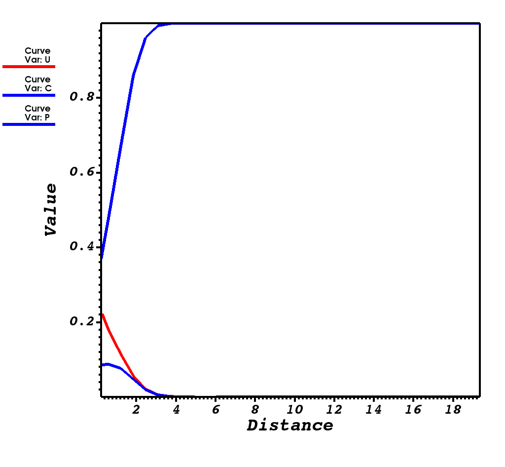
(a) s = 5

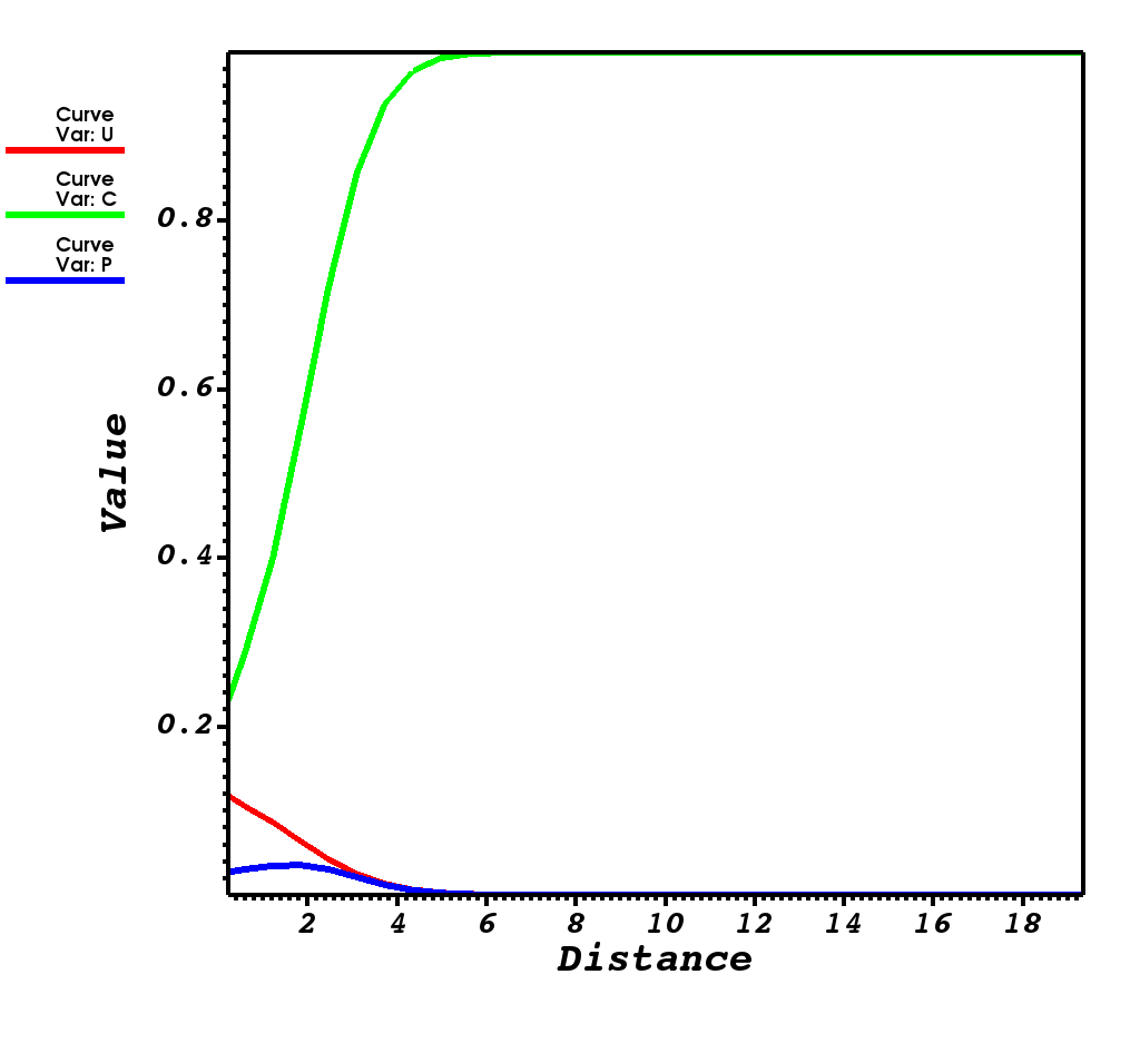
(b) t = 15

(c) t = 25

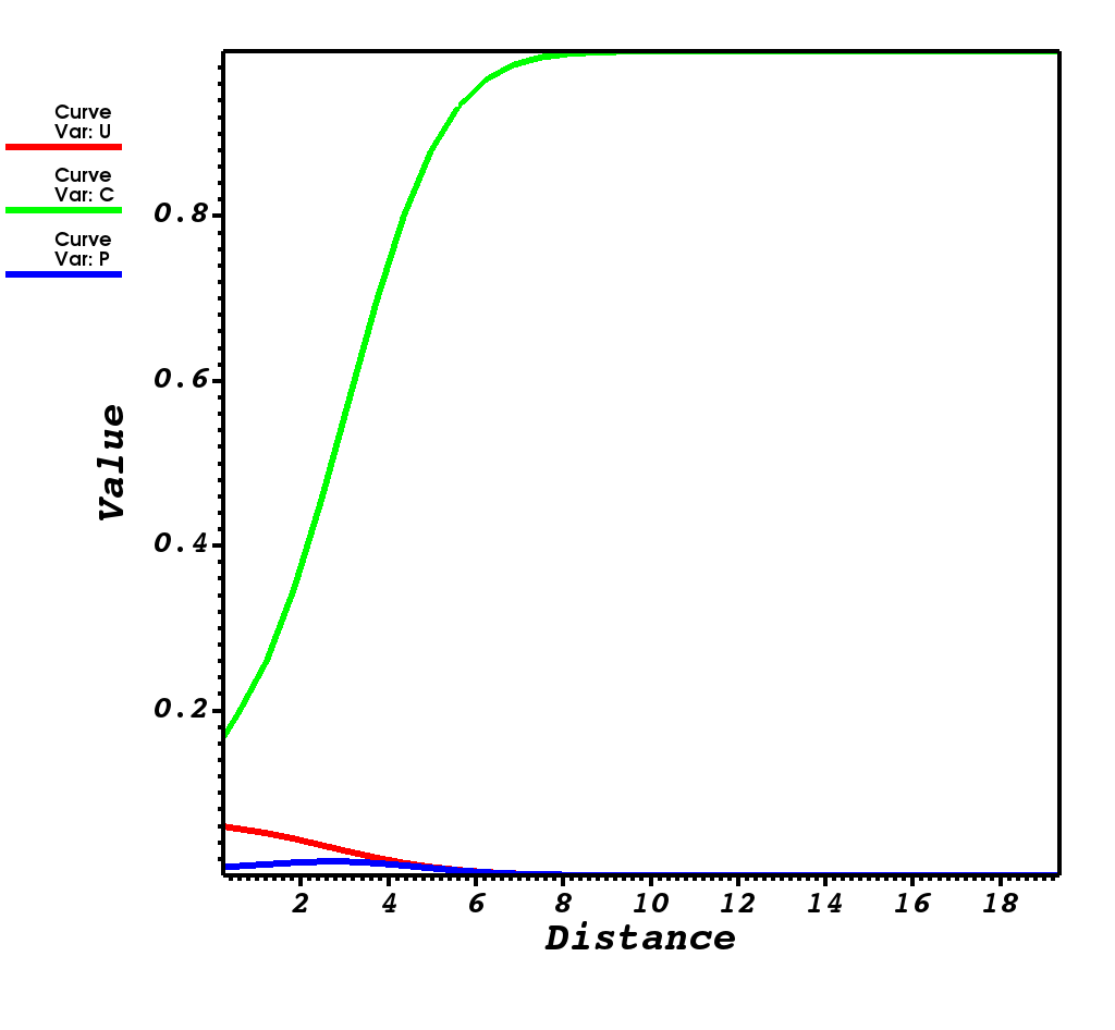
(d) t = 35

Figure 1: The effect of the proliferation rate on cancer cell invasion $u$, connective tissue $c$ and protease $p$ at different time steps, $t=5,15,25,35$ for $\mu=10^{-10}$.

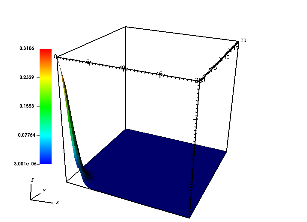
(a) t = 5

(b) t = 15

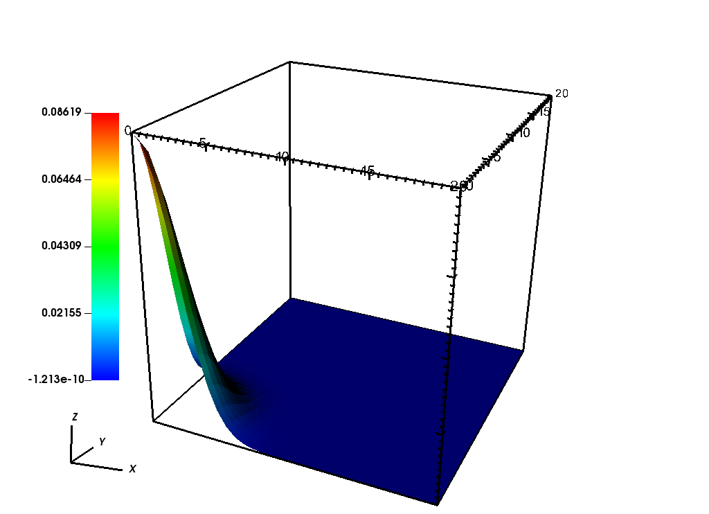
(c) t = 25

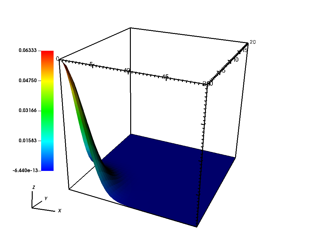
(d) t = 35

Figure 2: The snapshots of cancer cell invasion $u$ for $\mu=10^{-10}$, the maximum amount of cancer cells decreasing from left to right is 0.3106, 0.1348, 0.08619, and 0.06333.

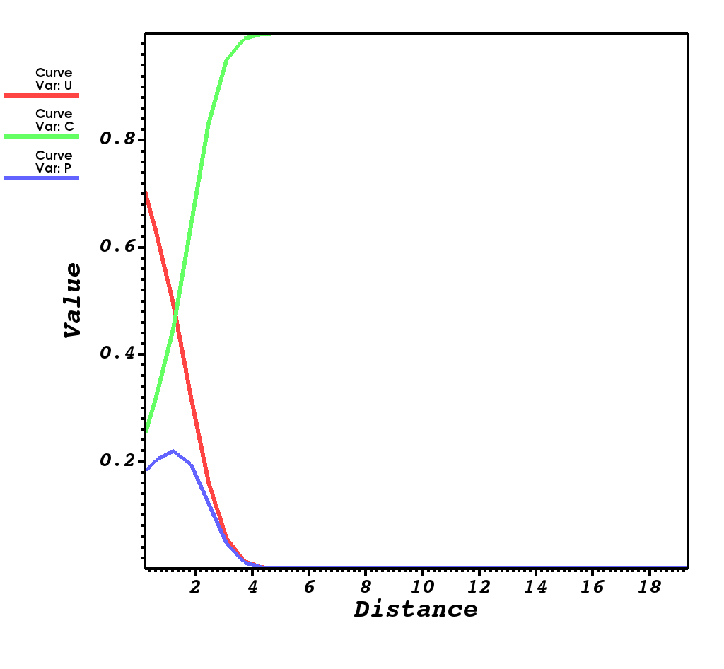
(a) t = 5

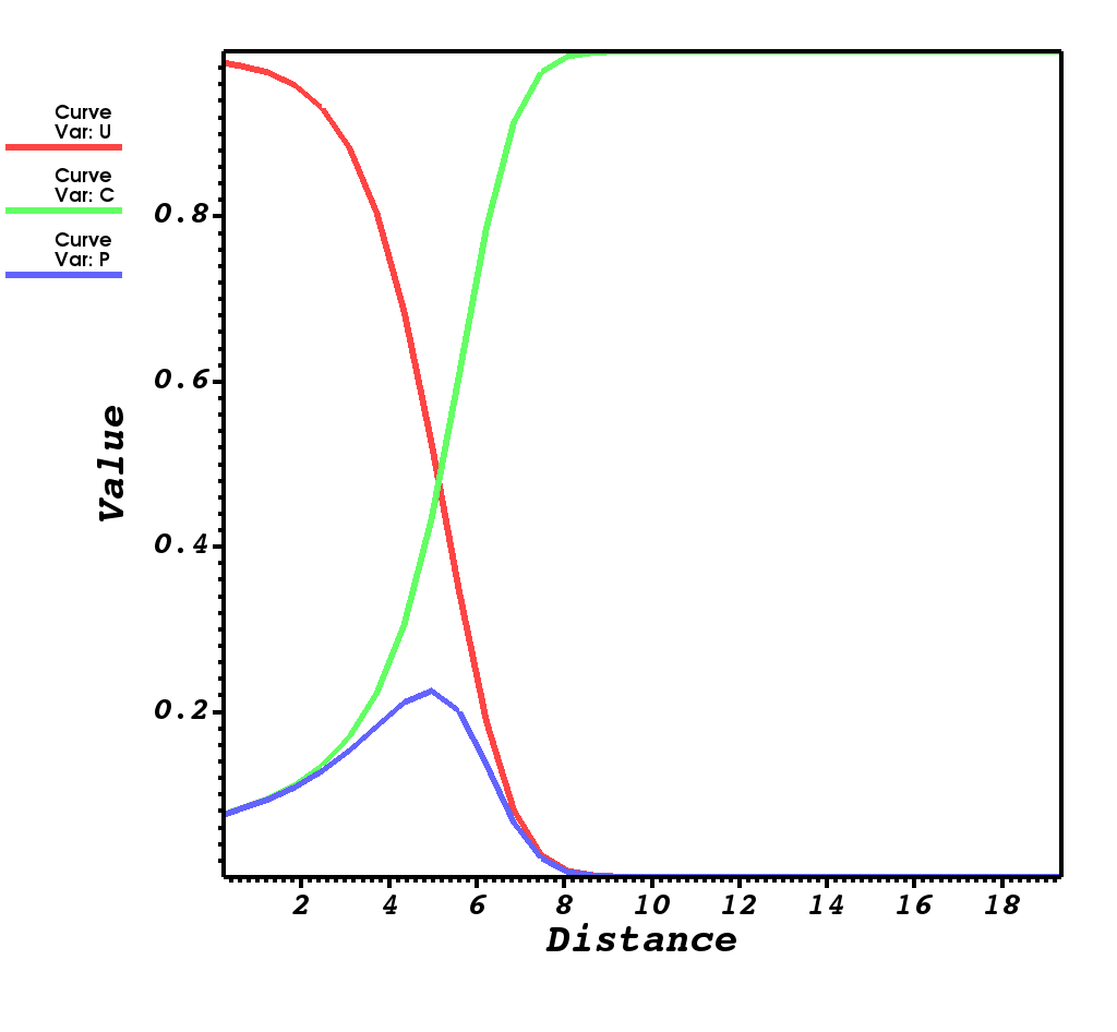
(b) t = 15

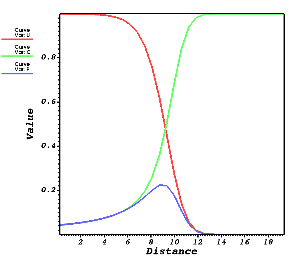
(c) t = 25

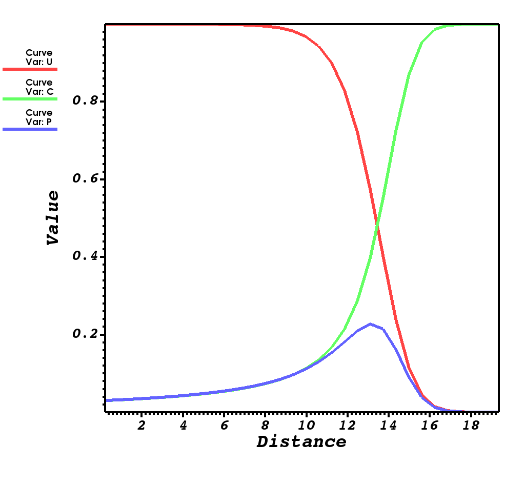
(d) t = 35

Figure 3: The effect of proliferation rate on cancer cell invasion $u$, connective tissue $c$ and protease $p$ at different time steps, $t=5,15,25,35$ for $\mu=0.5$.

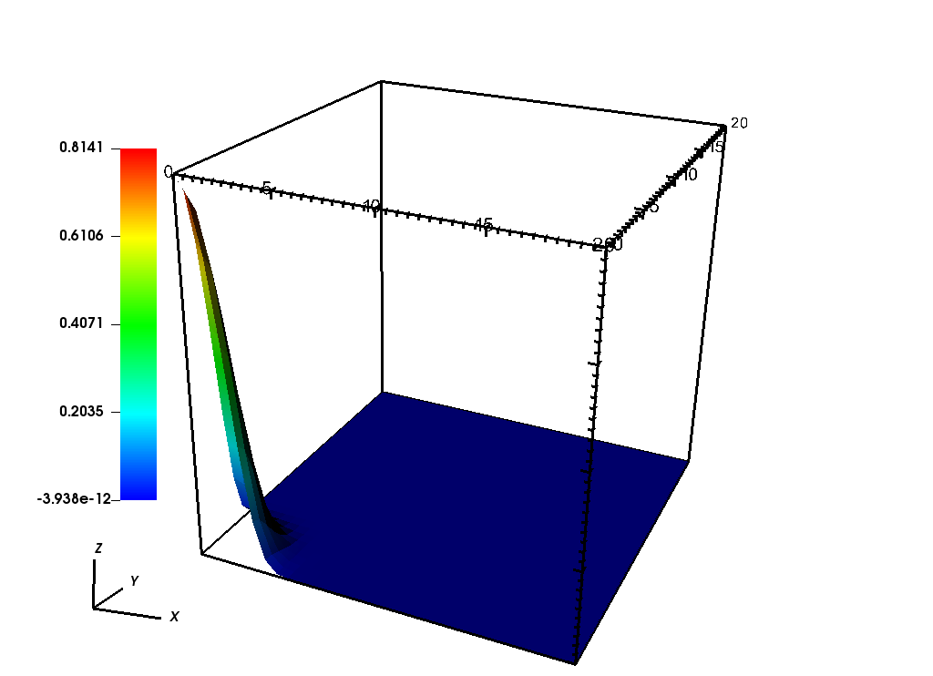
(a) t = 5

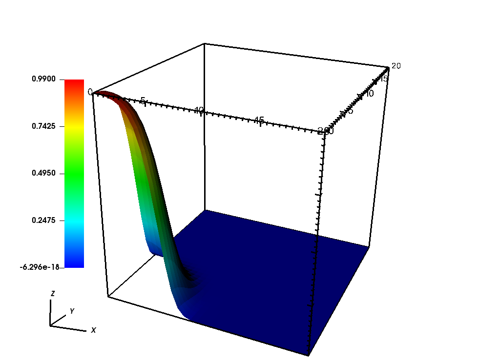
(b) t = 15

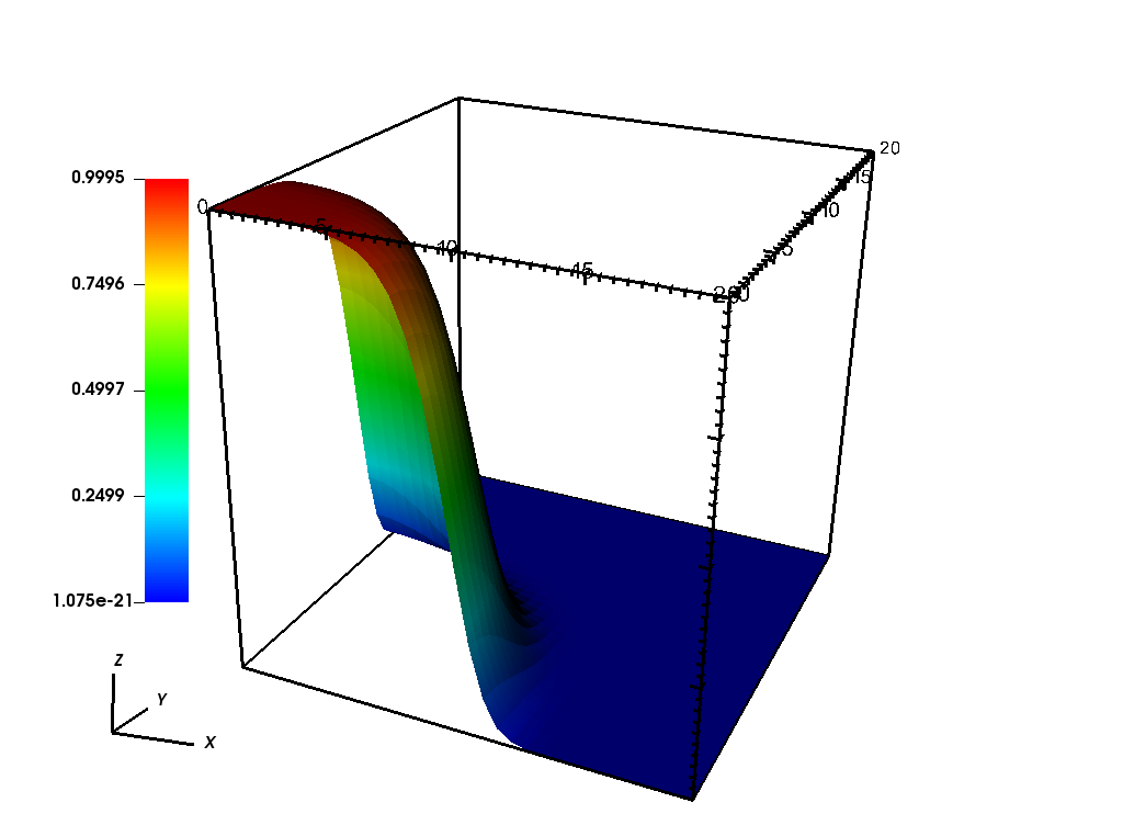
(c) t = 25

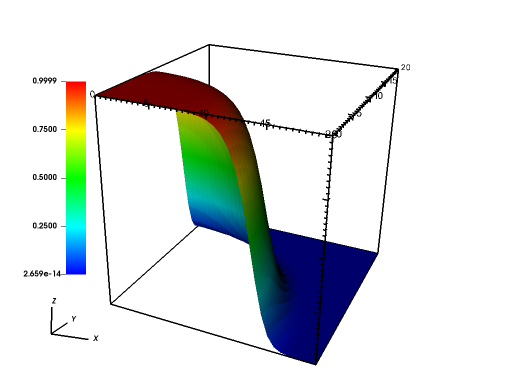
(d) t = 35

Figure 4: The snapshots of cancer cell invasion $u$ for $\mu=0.5$.

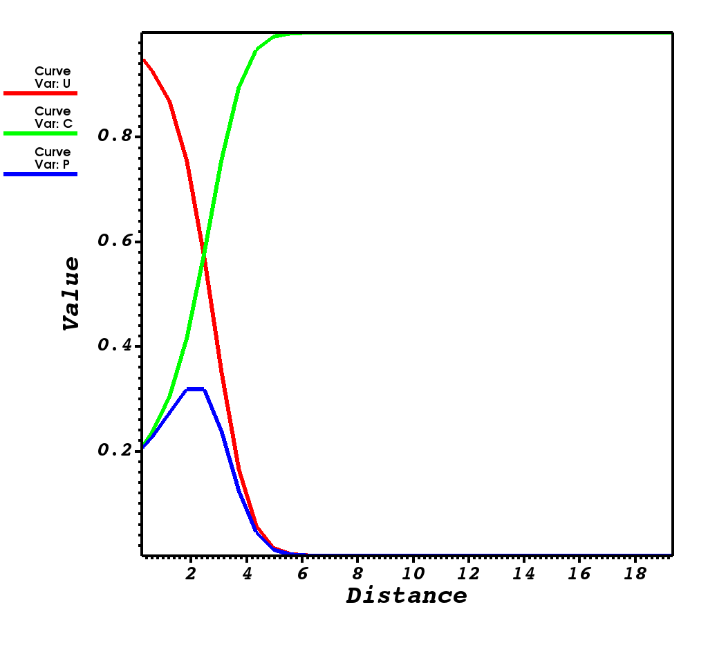
(a) t = 5

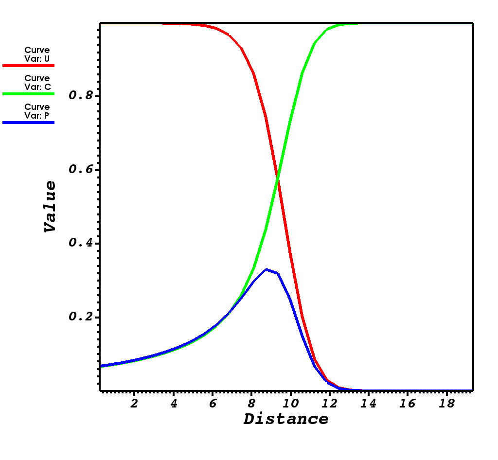
(b) t = 15

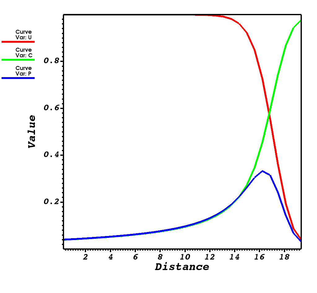
(c) t = 25

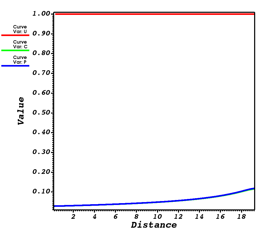
(d) t = 35

Figure 5: The effect of proliferation rate on cancer cell invasion, connective tissue and protease at different time steps, $t=5,15,25,35$ for $\mu=1.0$.

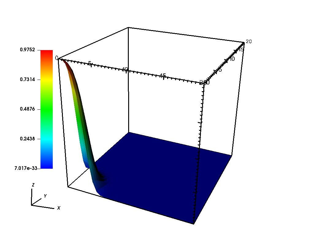
(a) t = 5

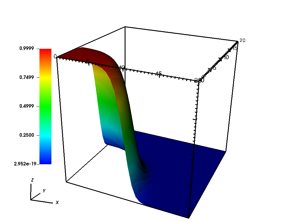
(b) t = 15

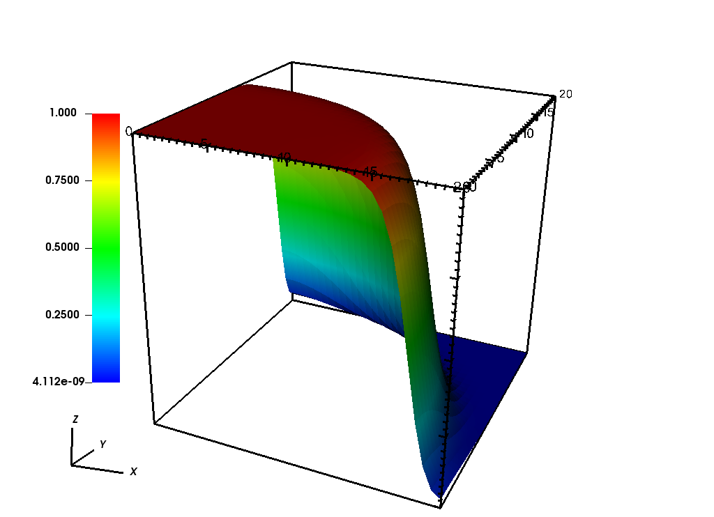
(c) t = 25

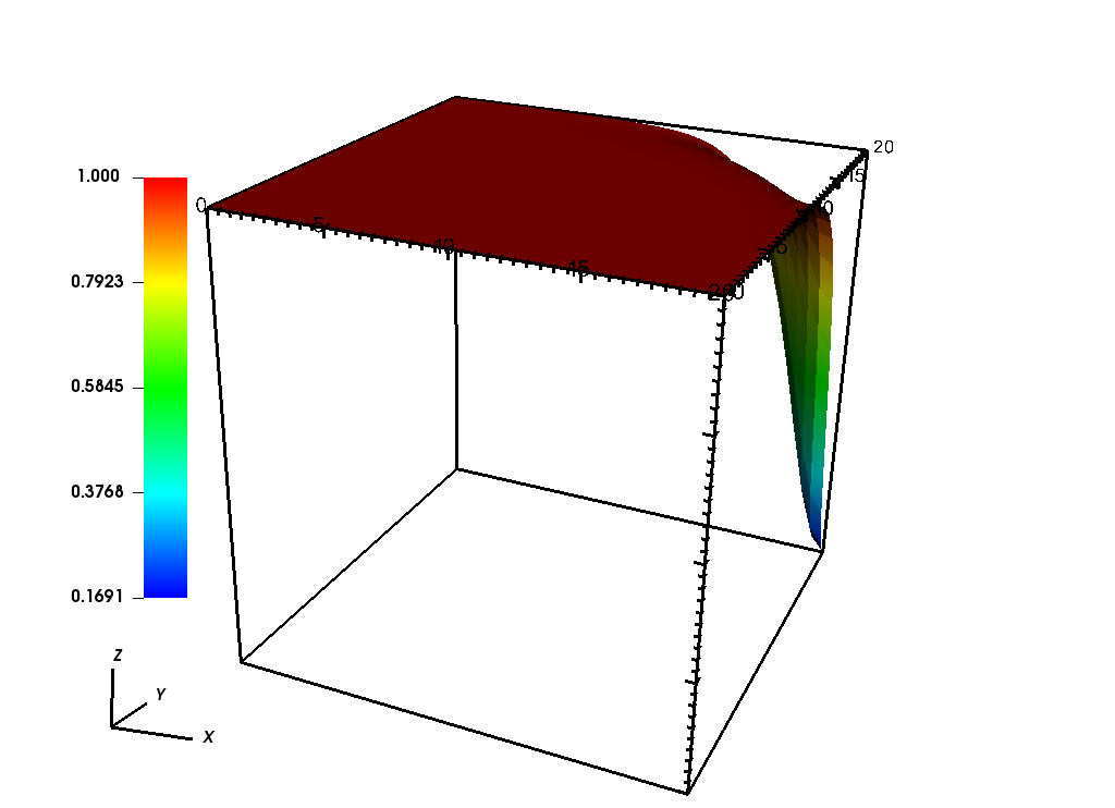
(d) t = 35

Figure 6: The snapshots of cancer cell invasion $u$ for $\mu=1.0$.

4.3 Effects of the haptotactic coefficient $\chi$

In this subsection, we consider the effect of the haptotactic coefficient on the connective cells degeneration by varying $\chi$. We choose $\chi=0.25,0.75,1.25$ with small proliferation rate $\mu=0.01$, diffusion coefficient $\alpha^{-1}=0.1$ and $\varepsilon=0.2$. The effects of haptotactic coefficient at different time instances are depicted in Figs. 7–12. Starting with $\chi=0.25$, the snapshot at $t=5$ shows that the cancer cells reduce at the origin and start migrating towards the direction of the gradient of connective tissue. The migration of the cancer cells becomes more clear and the effect of haptotaxis can be clearly seen at $t=5$ in Fig. 9 and Fig. 10, where the small cluster of cancer cells is created and becomes larger by time. Increasing the amount of $\chi$ accelerates the cancer cells migration and the cancer cells should move toward the boundary of the domain quickly, but as we can see from Fig. 11 and Fig. 12, oscillations start at $t=5$ and the numerical simulation breaks down for $\chi=1.25$.

(a) t = 5

(b) t = 15

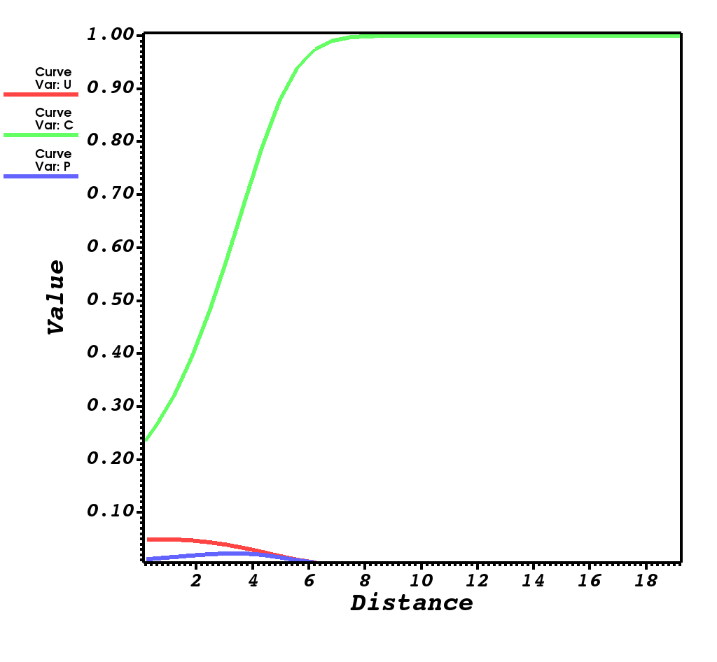
(c) t = 25

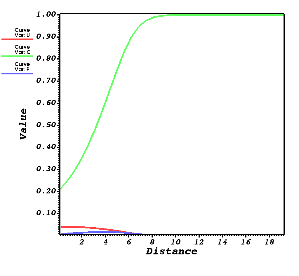
(d) t = 35

Figure 7: Haptotactic effect on cancer cell invasion, connective tissue and protease at different time steps, $t=5,15,25,35$ for $\chi=0.25$.

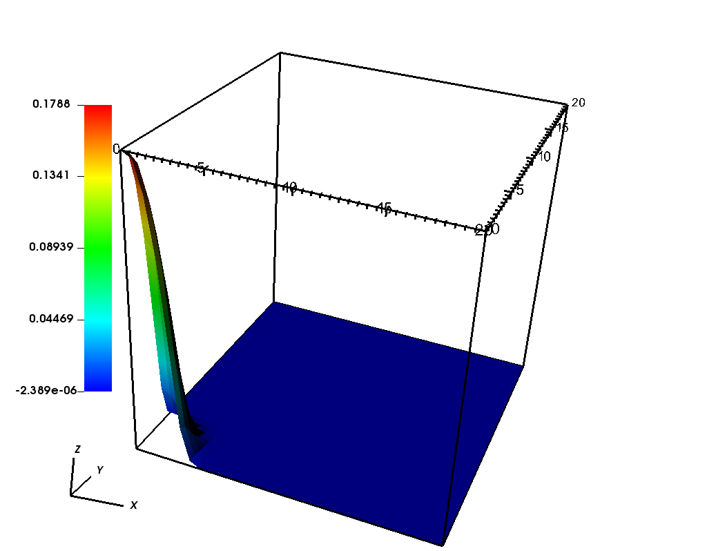
(a) t = 5

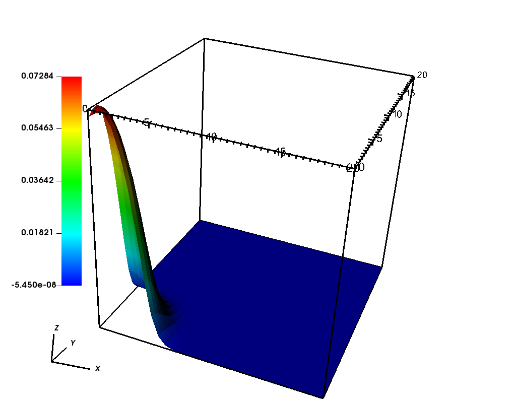
(b) t = 15

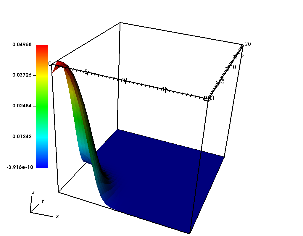
(c) t = 25

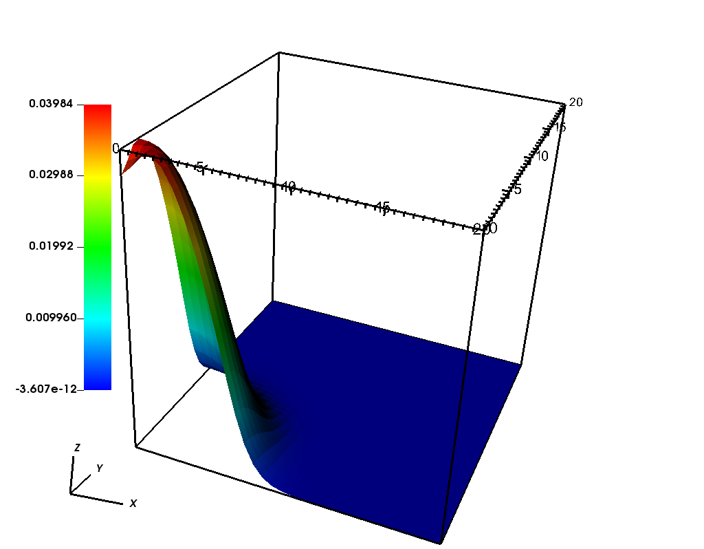
(d) t = 35

Figure 8: The snapshots of cancer cell invasion $u$ for $\chi=0.25$, the maximum amount of cancer cells decreasing from left to right is 0.1788, 0.07284, 0.04968, and 0.03984.

(a) t = 5

(b) t = 15

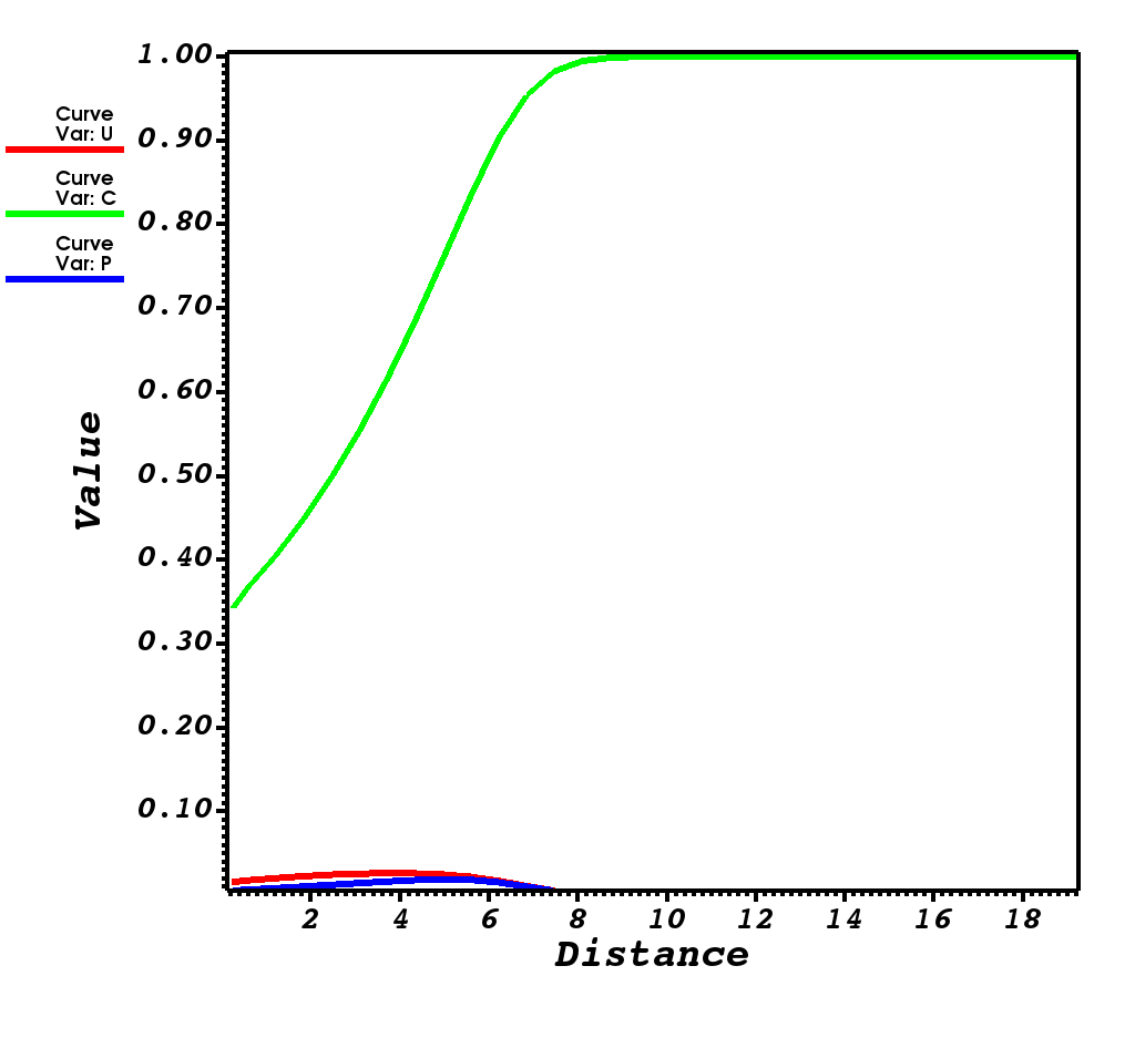
(c) t = 25

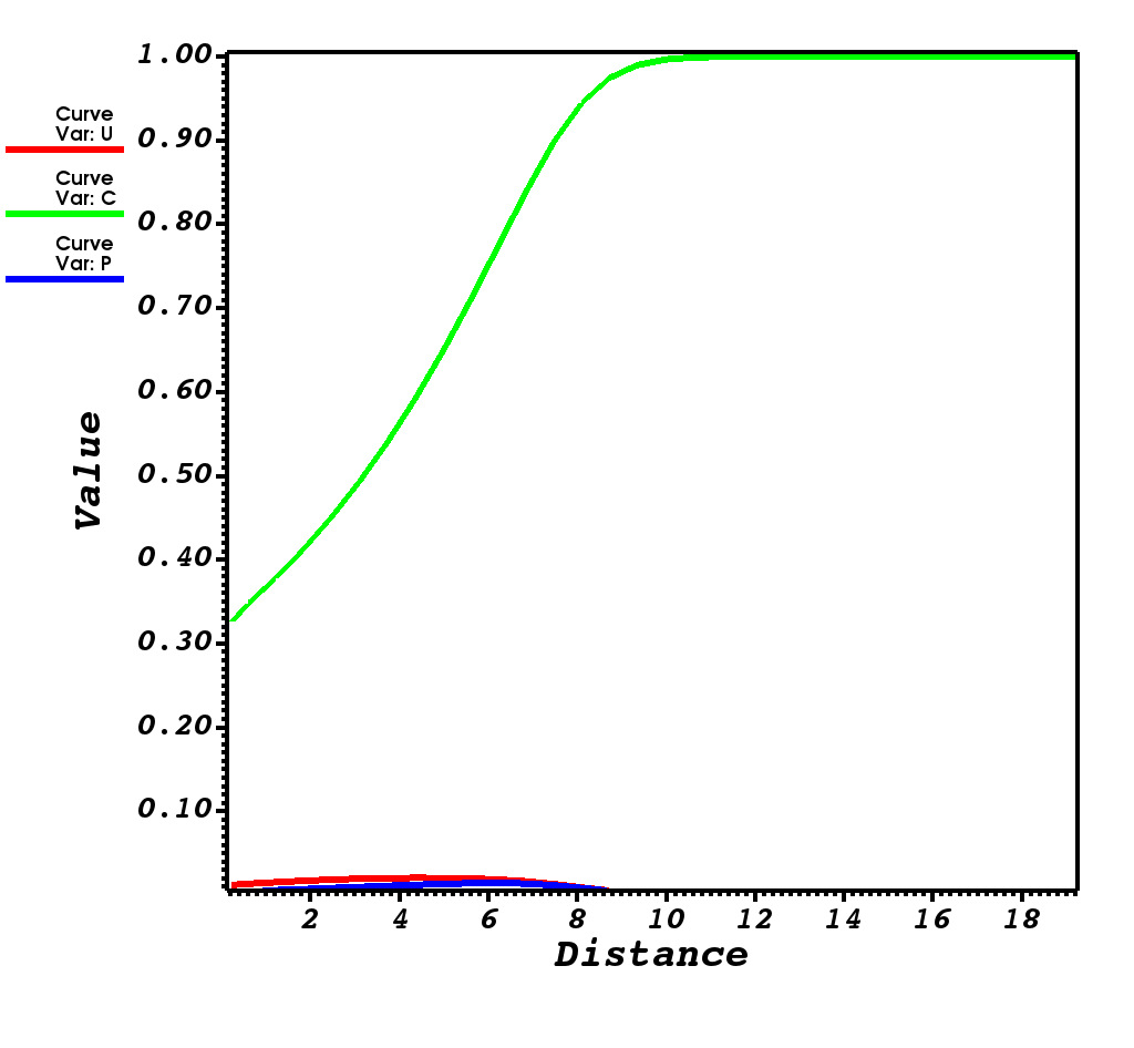
(d) t = 35

Figure 9: Haptotactic effect on cancer cell invasion, connective tissue and protease at different time steps, $t=5,15,25,35$ for $\chi=0.75$.

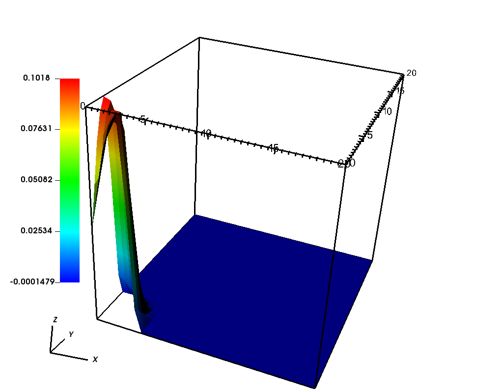
(a) t = 5

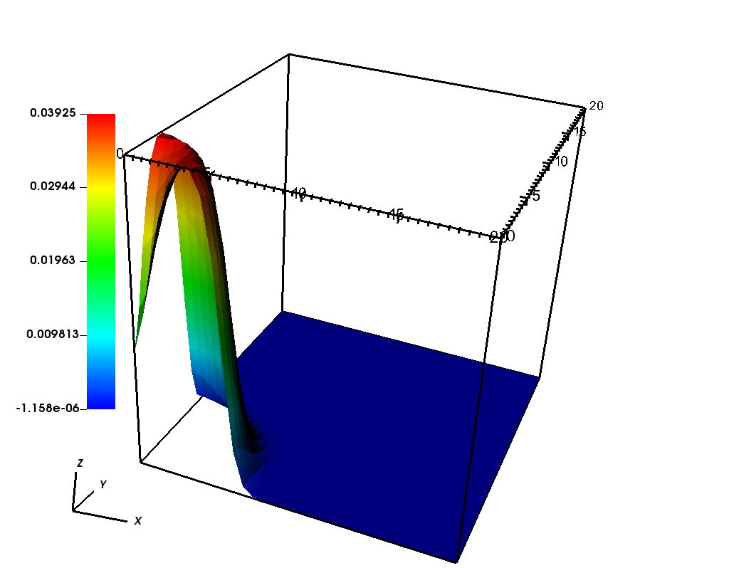
(b) t = 15

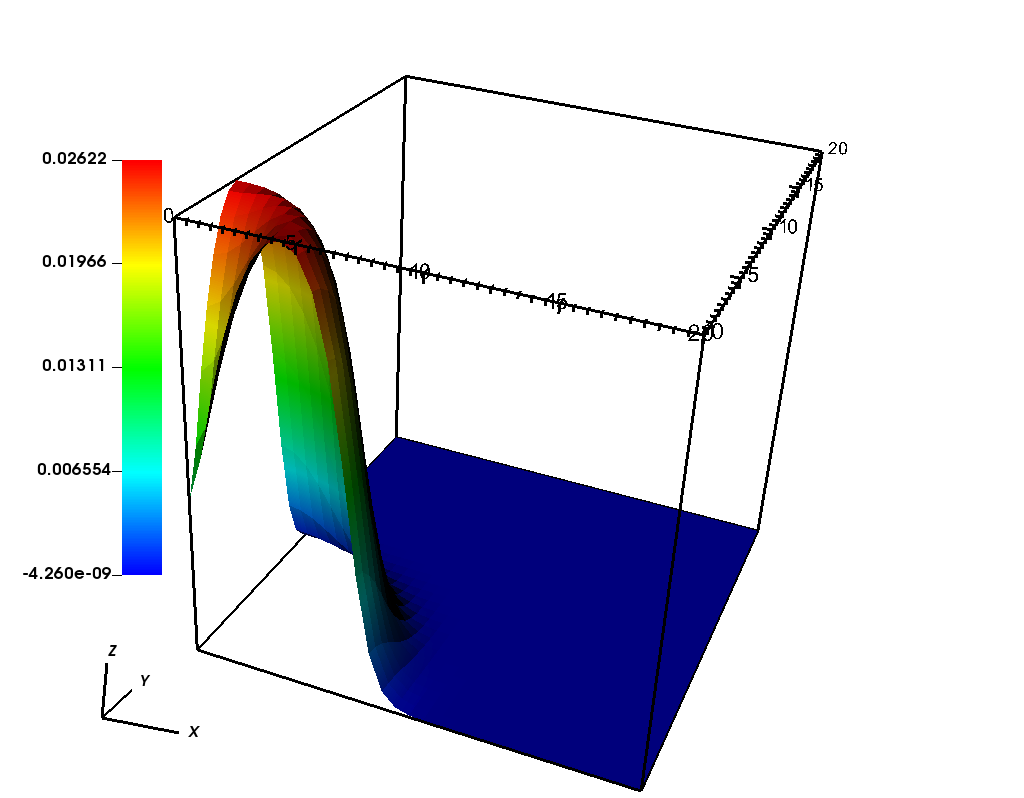
(c) t = 25

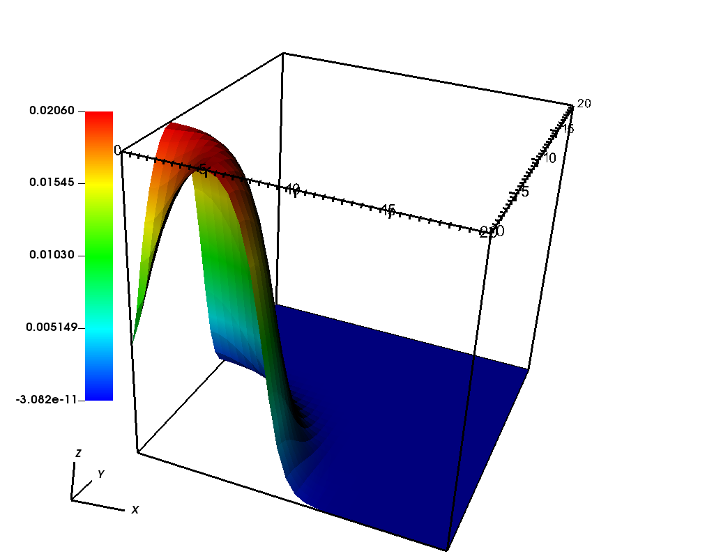
(d) t = 35

Figure 10: The snapshots of cancer cell invasion $u$ for $\chi=0.75$, the maximum amount of cancer cells decreasing from left to right is 0.1018, 0.03925, 0.02622, and 0.02060.

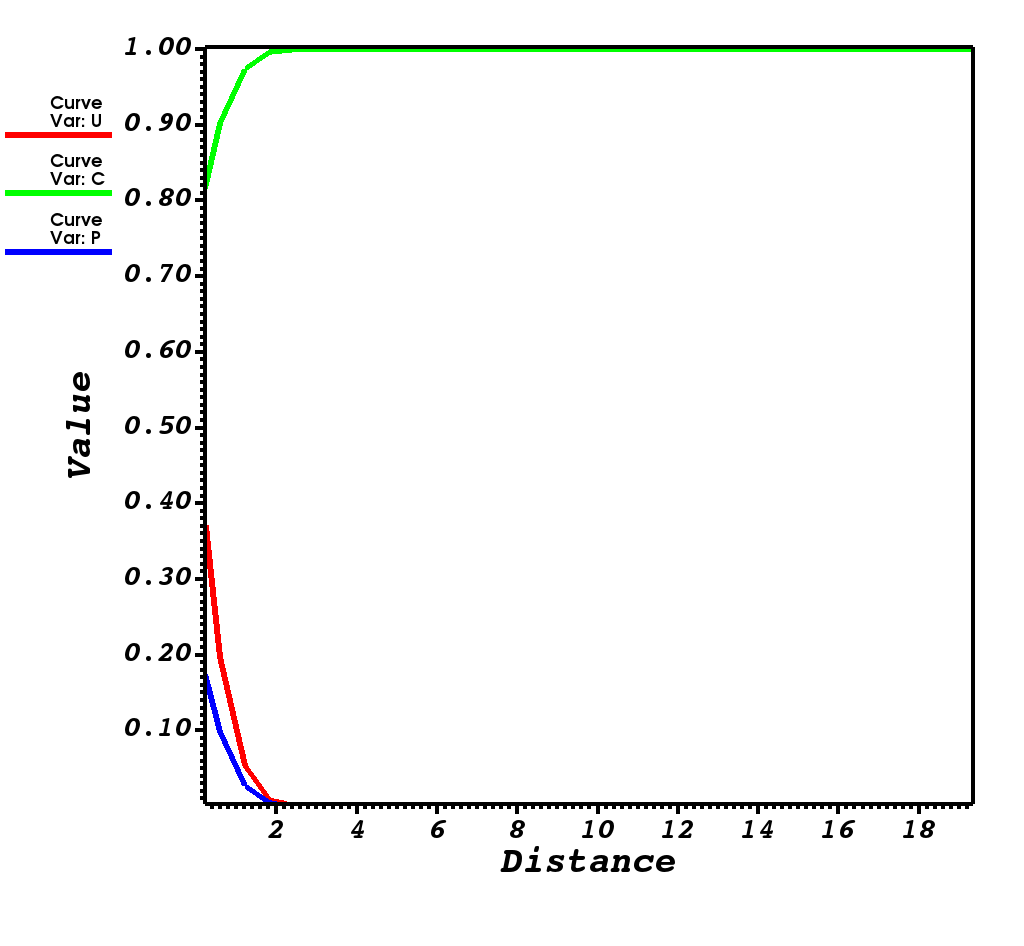
(a) t = 0

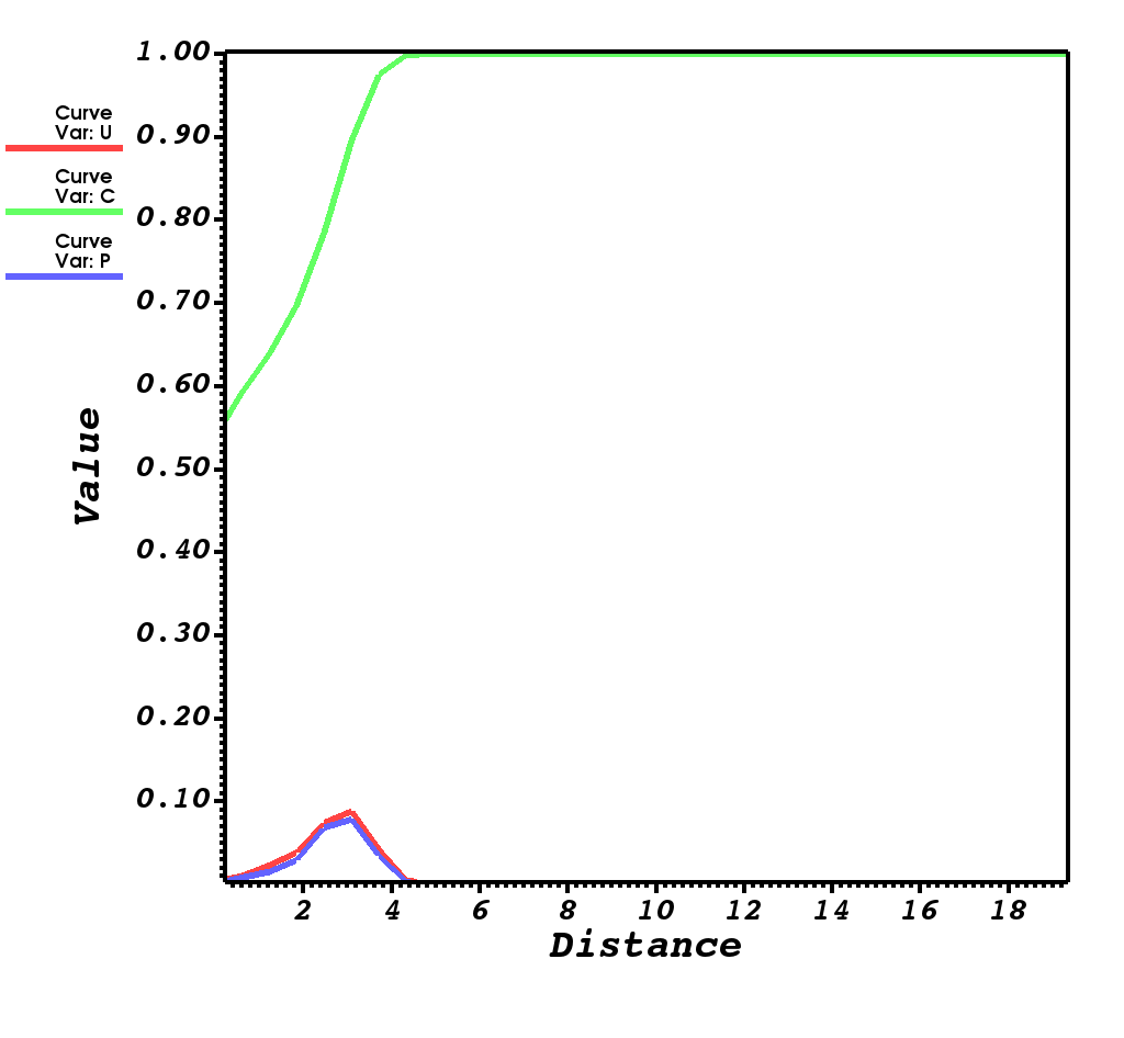
(b) t = 5

Figure 11: Haptotactic effect on cancer cell invasion, connective tissue and protease at different time steps, $t=0,5$ for $\chi=1.25$.

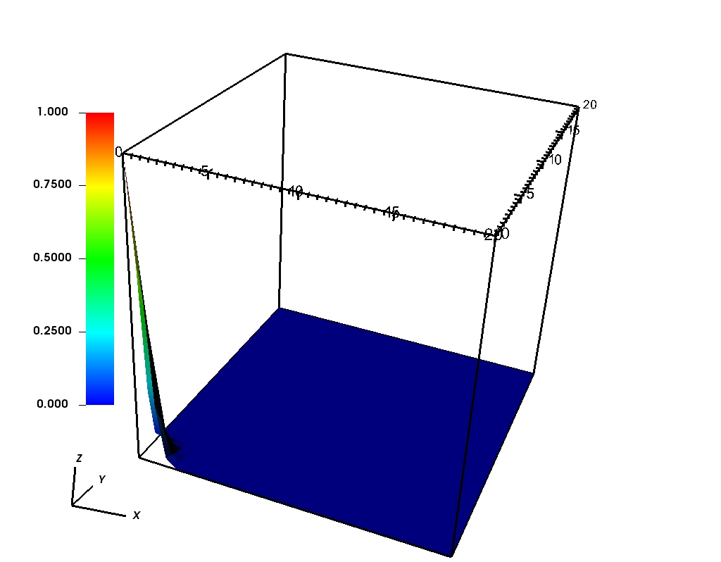
(a) t = 0

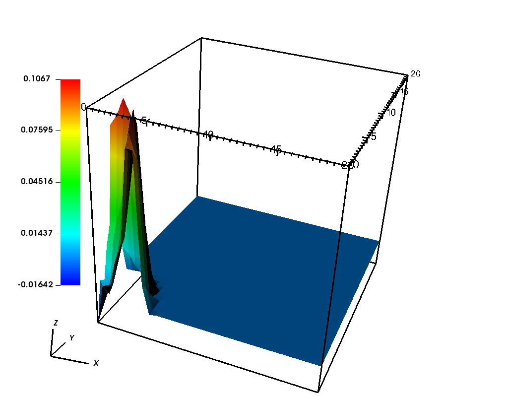
(b) t = 5

Figure 12: The snapshots of cancer cell invasion $u$ for $\chi=1.25$.

4.4 Identical proliferation and haptotactic coefficients

In this subsection, we consider the case when the proliferation rate is equal to haptotactic coefficient, i.e., $\mu=\chi=1$, and all other parameters are the same as in the previous subsections. As it can be seen from Figs. 13 and 14, due to the proliferation rate, the concentration of cancer growths quickly even from the beginning resulting from a high amount of haptotaxis, therefore the tumour migrates rapidly inside the domain and degrades the connective tissue in a much shorter amount of time.

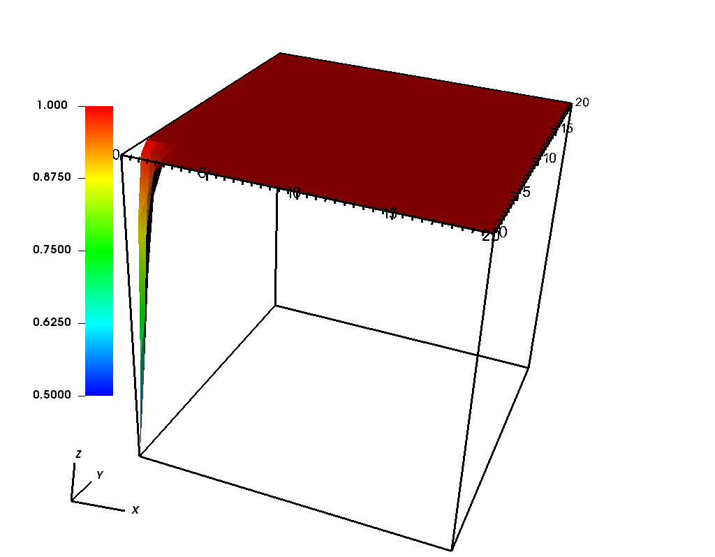
(a) t = 0

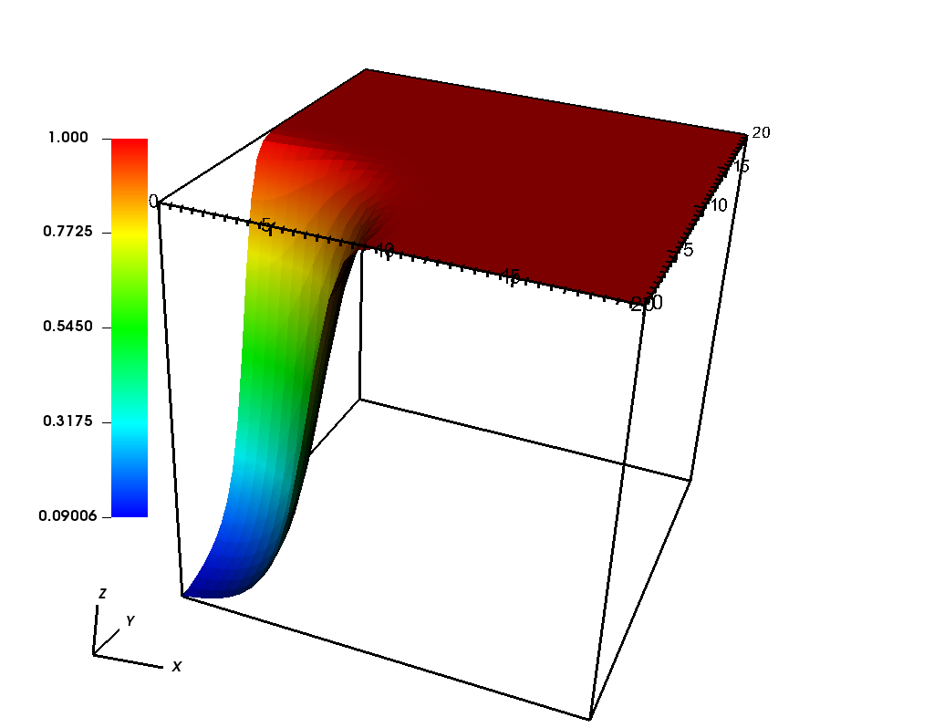
(b) t = 10

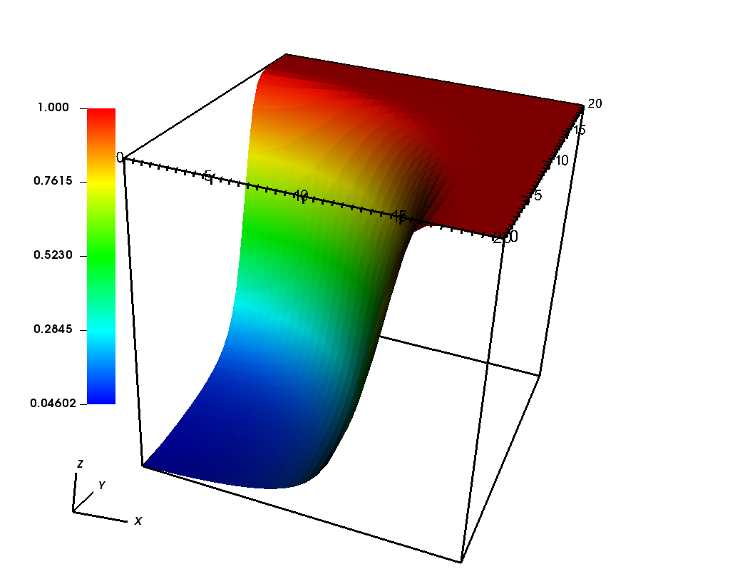
(c) t = 20

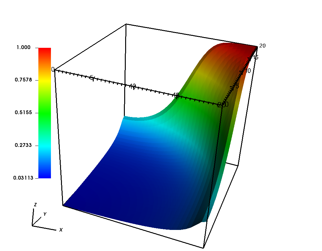
(d) t = 30

Figure 13: Degradation of connective tissue $c$ for $\chi=1.0,\mu=1.0$ at different time instances $t=0,10,20$ and 30.

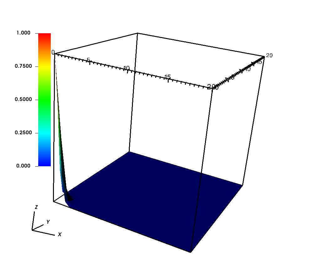
(a) t = 0

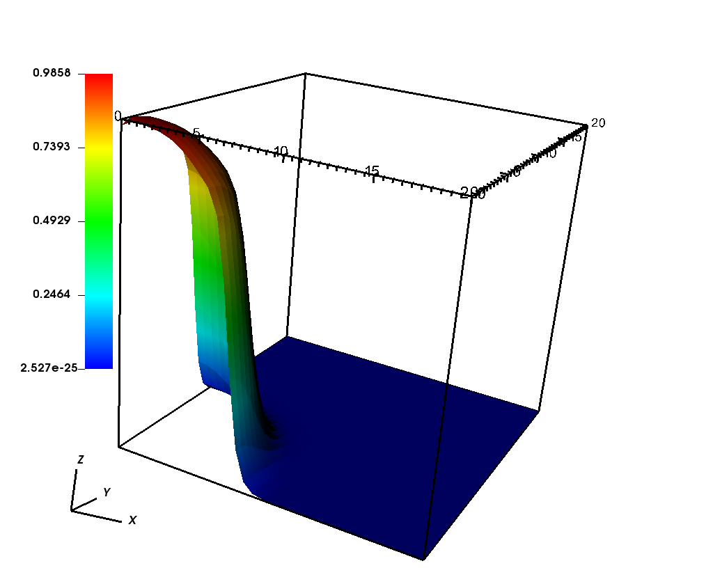
(b) t = 10

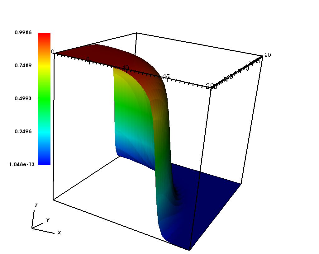
(c) t = 20

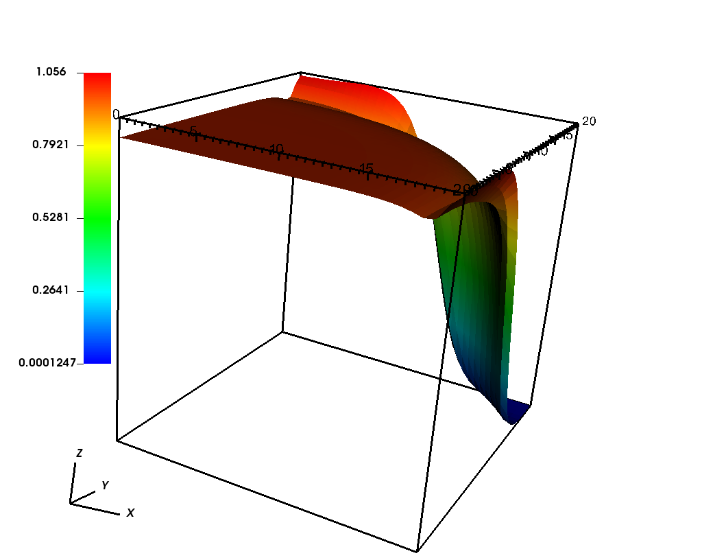
(d) t = 30

Figure 14: Invasion of cancer cells $u$ for $\chi=1.0,\mu=1.0$ at different time instances $t=0,10,20$ and 30.

4.5 Three dimensional simulations

In this final subsection, we perform numerical simulations in three spatial dimensions to consider some more realistic movement. Here, the experiments are performed on a mesh with $32\,768$ hexahedral elements covering the domain $\Omega$. Figs. 15 and 16 show the snapshots of cancer cells and connective tissues for growth rate $\mu=1$ and haptotactic coefficient $\chi=1$. Further, we use the parameters $\alpha^{-1}=0.1$ and $\varepsilon=0.2$. As it can be seen, at $t=5$ the connective tissue covers the entire domain and only a small amount of cancer cells exists at the corner, by the time cancer cells growth and invade the domain of connective tissue quickly and by $t=35$ almost all the domain is occupied by cancer cells.

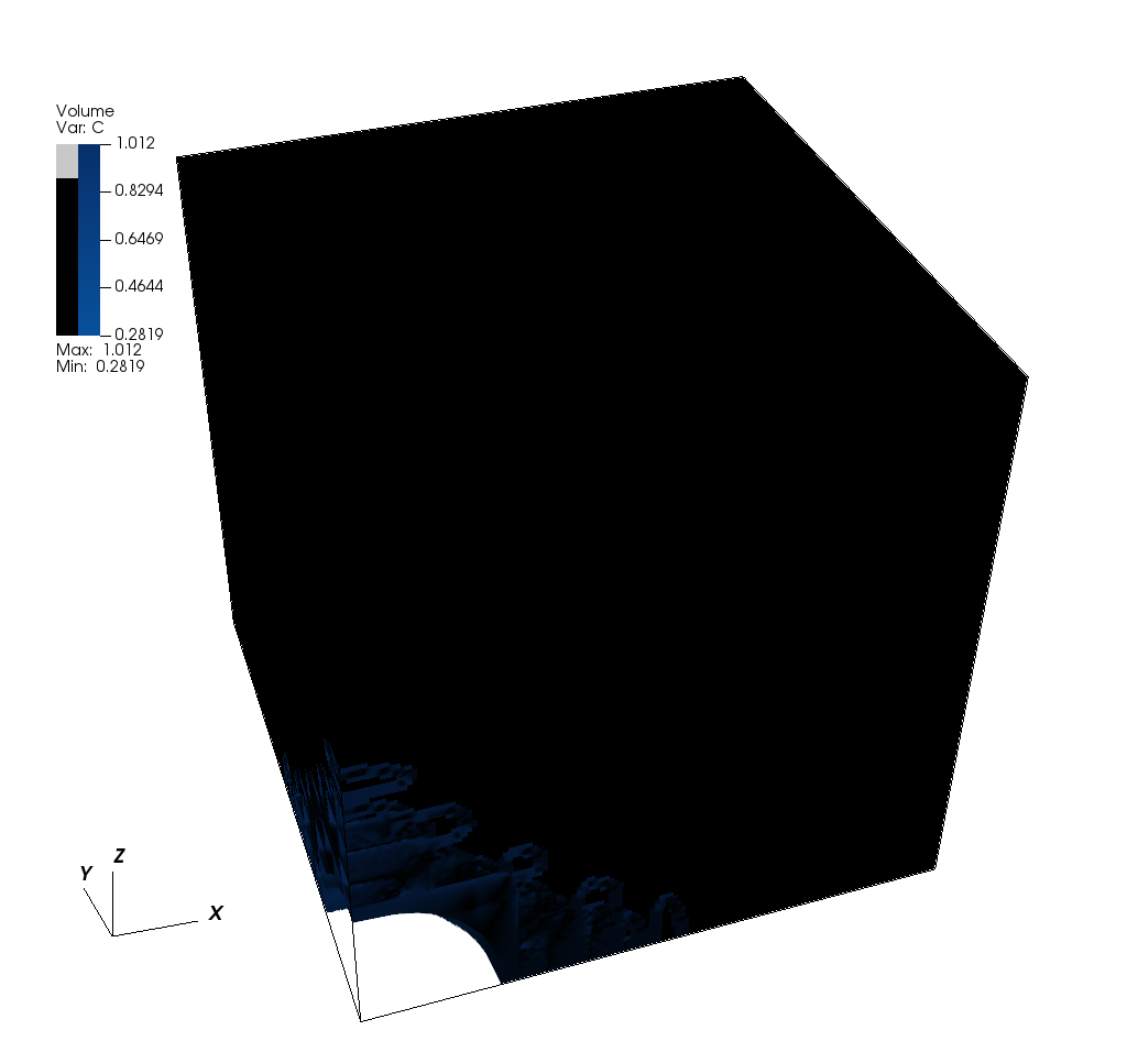
(a) t = 5

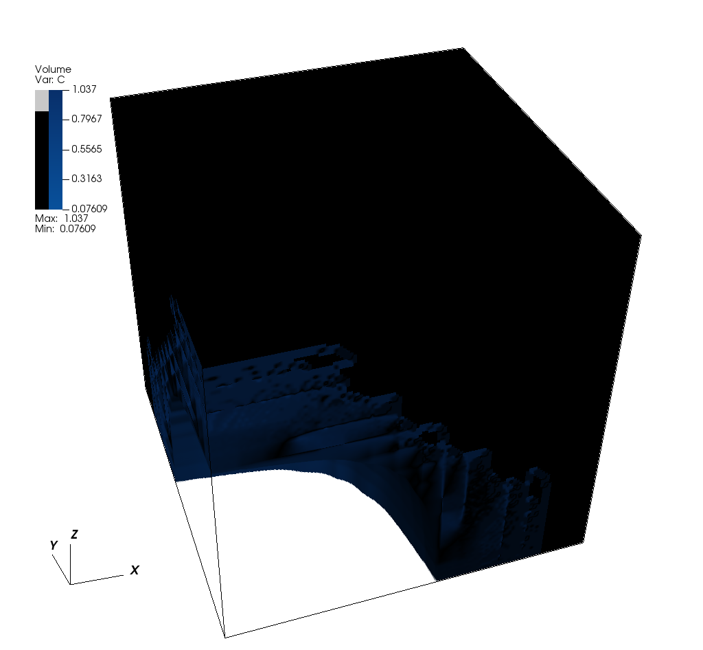
(b) t = 15

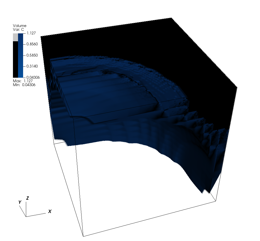
(c) t = 25

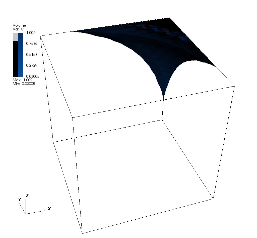
(d) t = 35

Figure 15: Degradation of connective tissue $c$ for $\chi=1.0,\mu=1.0$ at different time instances $t=5,15,25$ and 35.

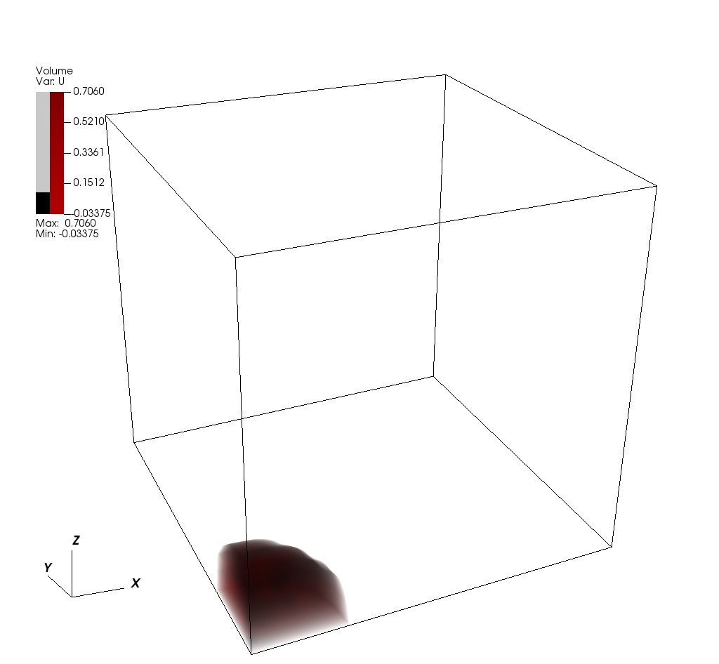
(a) t = 5

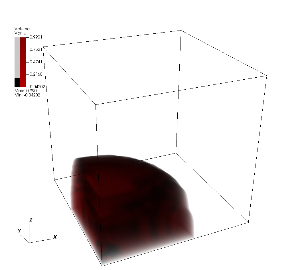
(b) t = 15

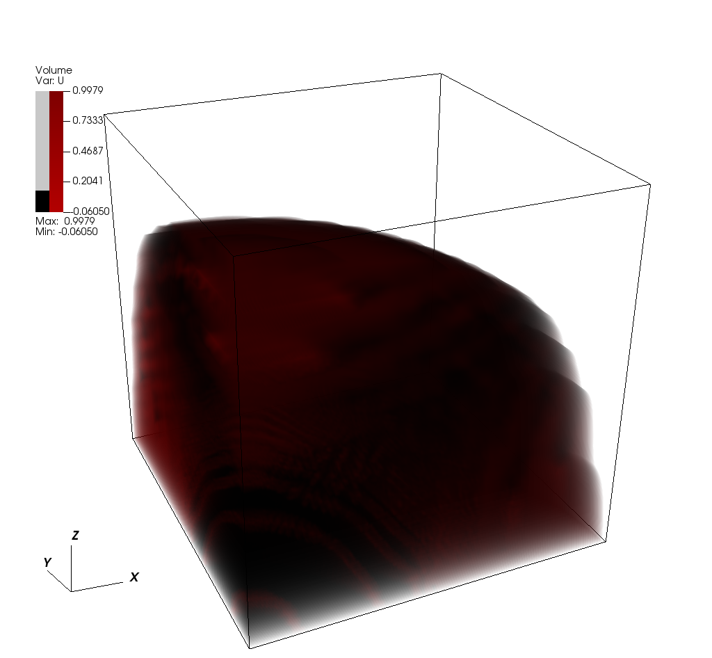
(c) t = 25

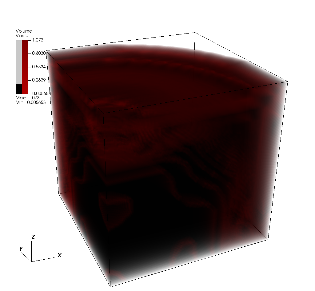
(d) t = 35

Figure 16: Invasion of cancer cells $u$ for $\chi=1.0,\mu=1.0$ at different time instances $t=5,15,25$ and 35.

5 Conclusions

In this paper, we established theoretical proofs, numerical algorithms, implementations and numerical simulations for a cancer invasion model. In our theoretical part, existence of global classical solutions in both two- and three-dimensional bounded domains were established. In the proofs, we employed the fact that the second and third equation in (1.1) at least regularize in time. For showing boundedness in $L^{\infty}$, the comparison principle allowed us to conclude boundedness in small time intervals, which then was iteratively applied to obtain the result also for larger times. For the spatial derivatives, we secondly applied a testing procedure for deriving estimates valid on small time intervals, again followed by an iteration procedure. Parabolic regularity theory yielded global existence of the solutions.

The numerical stability of the system heavily depends on the haptotactic coefficient $\chi$. By fixing proliferation rate $\mu$ and varying the $\chi$ one can make either the diffusion or transport of the cells dominant. The later usually gives rise to spurious oscillations or numerical blow up in the system. In order to study such properties, (1.1) was discretized using finite differences in time and Galerkin finite elements in space. A fixed-point scheme was designed to decouple the three equations, yielding a robust nonlinear procedure. These developments and their implementation allowed us to study numerically variations in $\mu$ and $\chi$ in two and three spatial dimensions and to illustrate our theoretical results.

As to future work, we notice that higher parameter variations resulting into convection-dominated regimes, require the design and implementation of stabilization methods such as streamline upwind Petrov–Galerkin stabilizing formulations or algebraic flux corrected transport.

References

• [1] A. Amoddeo. Adaptive grid modelling for cancer cells in the early stage of invasion. Comput. Math. Appl., 69(7):610–619, 2015.
• [2] A. R. Anderson. A hybrid mathematical model of solid tumour invasion: the importance of cell adhesion. Math. Med. Biol., 22(2):163–186, 2005.
• [3] A. R. A. Anderson, M. A. J. Chaplain, E. L. Newman, R. J. C. Steele, and A. M. Thompson. Mathematical modelling of tumour invasion and metastasis. Comput. Math. Methods Med., 2(2):129–154, 2000.
• [4] D. Arndt, W. Bangerth, T. C. Clevenger, D. Davydov, M. Fehling, D. Garcia-Sanchez, G. Harper, T. Heister, L. Heltai, M. Kronbichler, R. M. Kynch, M. Maier, J.-P. Pelteret, B. Turcksin, and D. Wells. The deal.II library, version 9.1. J. Numer. Math., 27(4):203–213, 2019.
• [5] D. Arndt, W. Bangerth, D. Davydov, T. Heister, L. Heltai, M. Kronbichler, M. Maier, J.-P. Pelteret, B. Turcksin, and D. Wells. The deal.II finite element library: Design, features, and insights. Comput. Math. Appl., 81:407–422, 2021.
• [6] S. Aznavoorian, M. L. Stracke, H. Krutzsch, E. Schiffmann, and L. A. Liotta. Signal transduction for chemotaxis and haptotaxis by matrix molecules in tumor cells. J. Cell Biol., 110(4):1427–1438, 1990.
• [7] M. A. J. Chaplain and G. Lolas. Mathematical modelling of cancer cell invasion of tissue: the role of the urokinase plasminogen activation system. Math. Models Methods Appl. Sci., 15:1685–1734, 2005.
• [8] M. A. J. Chaplain and G. Lolas. Mathematical modelling of cancer invasion of tissue: dynamic heterogeneity. Netw. Heterog. Media, 1(3):399–439, 2006.
• [9] M. Chapwanya, J. M.-S. Lubuma, and R. E. Mickens. Positivity-preserving nonstandard finite difference schemes for cross-diffusion equations in biosciences. Comput. Math. Appl., 68(9):1071–1082, 2014.
• [10] A. Chertock and A. Kurganov. A second-order positivity preserving central-upwind scheme for chemotaxis and haptotaxis models. Numer. Math., 111(2):169–205, 2008.
• [11] P. G. Ciarlet. The finite element method for elliptic problems. Studies in Mathematics and its Applications, Vol. 4. North-Holland Publishing Co., Amsterdam-New York-Oxford, 1978.
• [12] L. Corrias, B. Perthame, and H. Zaag. Global solutions of some chemotaxis and angiogenesis systems in high space dimensions. Milan J. Math., 72:1–28, 2004.
• [13] T. A. Davis and I. S. Duff. An unsymmetric-pattern multifrontal method for sparse LU factorization. SIAM J. Matrix Anal. Appl., 18(1):140–158, 1997.
• [14] P. Domschke, D. Trucu, A. Gerisch, and M. A. J. Chaplain. Mathematical modelling of cancer invasion: implications of cell adhesion variability for tumour infiltrative growth patterns. J. Theoret. Biol., 361:41–60, 2014.
• [15] Y. Epshteyn. Discontinuous Galerkin methods for the chemotaxis and haptotaxis models. J. Comput. Appl. Math., 224(1):168–181, 2009.
• [16] A. Friedman. Partial Differential Equations. R. E. Krieger Pub. Co, Huntington, N.Y, 1976.
• [17] M. Fuest. Global solutions near homogeneous steady states in a multidimensional population model with both predator- and prey-taxis. SIAM J. Math. Anal., 52(6):5865–5891, 2020.
• [18] A. Gerisch and M. A. J. Chaplain. Mathematical modelling of cancer cell invasion of tissue: local and non-local models and the effect of adhesion. J. Theoret. Biol., 250(4):684–704, 2008.
• [19] Y. Giga and H. Sohr. Abstract ${L}^{p}$ estimates for the Cauchy problem with applications to the Navier–Stokes equations in exterior domains. J. Funct. Anal., 102(1):72–94, 1991.
• [20] D. Hanahan and R. A. Weinberg. The hallmarks of cancer. Cell, 100(1):57–70, 2000.
• [21] M. Khalsaraei, S. Heydari, and L. D. Algoo. Positivity preserving nonstandard finite difference schemes applied to cancer growth model. J. Cancer Treat. Res., 4(4):27–33, 2016.
• [22] M. Kolev and B. Zubik-Kowal. Numerical solutions for a model of tissue invasion and migration of tumour cells. Comput. Math. Methods Med., 2011, 2011.
• [23] O. A. Ladyženskaja, V. A. Solonnikov, and N. N. Ural’ceva. Linear and quasi-linear equations of parabolic type. Number 23 in Translations of Mathematical Monographs. American Mathematical Soc, Providence, RI, 1988. Translated from the Russian by S. Smith.
• [24] J. Lankeit and M. Winkler. Facing low regularity in chemotaxis systems. Jahresber. Dtsch. Math.-Ver., 122:35–64, 2019.
• [25] G. M. Lieberman. Hölder continuity of the gradient of solutions of uniformly parabolic equations with conormal boundary conditions. Ann. Mat. Pura Appl. (4), 148:77–99, 1987.
• [26] G. M. Lieberman. Second order parabolic differential equations. World Scientific Publishing Co., Inc., River Edge, NJ, 1996.
• [27] G. Liţcanu and C. Morales-Rodrigo. Asymptotic behavior of global solutions to a model of cell invasion. Math. Models Methods Appl. Sci., 20(9):1721–1758, 2010.
• [28] J. S. Lowengrub, H. B. Frieboes, F. Jin, Y.-L. Chuang, X. Li, P. Macklin, S. M. Wise, and V. Cristini. Nonlinear modelling of cancer: bridging the gap between cells and tumours. Nonlinearity, 23(1):R1–R91, 2010.
• [29] B. P. Marchant, J. Norbury, and A. J. Perumpanani. Travelling shock waves arising in a model of malignant invasion. SIAM J. Appl. Math., 60(2):463–476, 2000.
• [30] B. P. Marchant, J. Norbury, and J. A. Sherratt. Travelling wave solutions to a haptotaxis-dominated model of malignant invasion. Nonlinearity, 14(6):1653–1671, 2001.
• [31] L. Nirenberg. On elliptic partial differential equations. Ann. Della Scuola Norm. Super. Pisa - Cl. Sci., Ser. 3, 13(2):115–162, 1959.
• [32] A. J. Perumpanani and H. M. Byrne. Extracellular matrix concentration exerts selection pressure on invasive cells. Eur. J. Cancer, 35(8):1274–1280, 1999.
• [33] A. J. Perumpanani, J. A. Sherratt, J. Norbury, and H. M. Byrne. A two parameter family of travelling waves with a singular barrier arising from the modelling of extracellular matrix mediated cellular invasion. Phys. D, 126(3-4):145–159, 1999.
• [34] M. Rascle and C. Ziti. Finite time blow-up in some models of chemotaxis. J. Math. Biol., 33(4):388–414, 1995.
• [35] N. Sfakianakis and M. A. J. Chaplain. Mathematical modelling of cancer invasion: A review. In International Conference by Center for Mathematical Modeling and Data Science, Osaka University, pages 153–172. Springer, 2020.
• [36] R. Strehl, A. Sokolov, D. Kuzmin, D. Horstmann, and S. Turek. A positivity-preserving finite element method for chemotaxis problems in 3D. J. Comput. Appl. Math., 239:290–303, 2013.
• [37] C. Surulescu and M. Winkler. Does indirectness of signal production reduce the explosion-supporting potential in chemotaxis–haptotaxis systems? Global classical solvability in a class of models for cancer invasion (and more). Eur. J. Appl. Math, 32(4):618–651, 2021.
• [38] Y. Tao and M. Winkler. Energy-type estimates and global solvability in a two-dimensional chemotaxis-haptotaxis model with remodeling of non-diffusible attractant. J. Differential Equations, 257(3):784–815, 2014.
• [39] Y. Tao and G. Zhu. Global solution to a model of tumor invasion. Appl. Math. Sci, 1(48):2385–2398, 2007.
• [40] J. Valenciano and M. A. J. Chaplain. Computing highly accurate solutions of a tumour angiogenesis model. Math. Models Methods Appl. Sci., 13(05):747–766, 2003.
• [41] Ch. Walker and G. F. Webb. Global existence of classical solutions for a haptotaxis model. SIAM J. Math. Anal., 38(5):1694–1713, 2007.
• [42] T. Wick. Solving monolithic fluid-structure interaction problems in arbitrary Lagrangian Eulerian coordinates with the deal.II library. Archive of Numerical Software, 1:1–19, 2013.
• [43] X. Zheng, S. Wise, and V. Cristini. Nonlinear simulation of tumor necrosis, neo-vascularization and tissue invasion via an adaptive finite-element/level-set method. Bull. Math. Biol., 67(2):211–259, 2005.