CellTypeGraph: A New Geometric Computer Vision Benchmark

Abstract

Classifying all cells in an organ is a relevant and difficult problem from plant developmental biology. We here abstract the problem into a new benchmark for node classification in a geo-referenced graph. Solving it requires learning the spatial layout of the organ including symmetries. To allow the convenient testing of new geometrical learning methods, the benchmark of Arabidopsis thaliana ovules is made available as a PyTorch data loader, along with a large number of precomputed features. Finally, we benchmark eight recent graph neural network architectures, finding that DeeperGCN currently works best on this problem.

1 Introduction

Understanding morphogenesis, the generation of form, remains a major challenge in biology. It requires a detailed quantitative description of the molecular and cellular processes of the underlying mechanism. 3D digital organs with cellular spatial resolution promise to help decipher the morphogenesis of complex organs in plants [33, 56, 37, 20]. They can be generated by 3D microscopic imaging followed by cell instance segmentation and tissue annotation. Plant organs lend themselves to this approach as they exhibit a relatively well-structured, layered organization and the tissues can be identified based on their positions and morphology. Thus, plant developmental biology is profiting from a growing body of 3D digital organs. However, automatic annotation [33, 41, 32] of different tissue types within an organ remains a major problem in the field, particularly for plant organs of complex cellular architecture and shape such as ovules of Arabidopsis thaliana [53].

In medical image analysis, the analogous problem of segmenting whole-body scans has been addressed successfully using 3D encoder-decoder CNN architectures [54, 26]. In the images of interest to plant morphogenesis, this straightforward approach does not work as well: here, the semantic classes lack distinctive local and texture features helpful for convolution based architectures [14]. Instead, the task requires very long-range spatial awareness and good geometrical reasoning. In response, here we cast the problem as a node classification task. To succeed, any approach requires informative input features, and indeed we show that a cell-adjacency graph with cell-level features is a powerful representation.

That said, our primary intent is twofold: first, to create a testing ground for machine learning on highly structured input. Indeed, it uniquely combines node classification typical of popular datasets [31, 15, 43] with the requirement to generalize across geo-referenced graphs like in Quantum Chemistry [38, 4, 58, 17]. Our second intent is, by allowing computer vision and machine learning scientists to work on this problem without having to deal with data-processing issues that actually take the most time in many applied projects, to channel the creativity and resourcefulness of our community to help solve a fascinating biological problem.

As a starting point, we present extensive experiments evaluating the performance of state-of-the-art and popular models.

In summary, we make the following contributions:

1. We propose a new benchmark for node classification in a geo-referenced graph. We release the benchmark dataset together with a ready-to-use PyTorch [34] data loader. The source-code and usage instructions are available at https://github.com/hci-unihd/celltype-graph-benchmark.

2. We run comparative experiments using state-of-the-art graph neural networks and offer a study of feature relevance.

3. We provide an extensive set of precomputed features and an additional set of ground truth labels.

1.1 Related work

Arguably the most popular type of dataset for node predictions is the family of citation datasets, such as Cora [31], CiteSeer [15] or PubMed [43]. Although the task is nominally identical, the learning task is here transductive, and the underlying topologies are extremely different. In our CellTypeGraph, the task is inductive, and nodes are geo-referenced with a limited variance in node degrees and no shortcuts between distant nodes. This is not typically the case in citation datasets. More closely related are other natural science datasets such as QM9 [38, 4] or ZINC [17], MoleculeNet [58]. Nodes here represent atoms and are geo-referenced. Nevertheless, they are, for the most part, interested in regression and classification of global graph properties.

The Open Graph Benchmark [21] contains a vast collection of datasets at different scales and also releases easy to use data loader and evaluation tools. As pointed out in [21], on many datasets the limited size, lack of agreed-upon train/val/test splits, and use of different metrics make it hard to measure progress in the field. In CellTypeGraph, we also release all tools required to ensure simple and reproducible experimentation. Moreover, we propose cross-validation [49] rather than a simple train/val/test split to further reducing sampling biases.

Motivated by the success of convolution neural networks, several graph neural network architectures attempt to generalize the same concept to non-grid structured data [25, 10, 19]. Those architectures and many more [52, 18, 59, 57, 7, 27, 28, 5] can be modeled as message passing [16], where messages built at the node level can be shared over the local neighborhood. In case of geo-referenced or spatial graphs, the node positions can be used to model the messages aggregations over the graph adjacency [8, 9]. Alternatively, others [42, 50], have obtained competitive results on molecular tasks by using only node positions and ignoring the graph adjacency.

2 CellTypeGraph benchmark

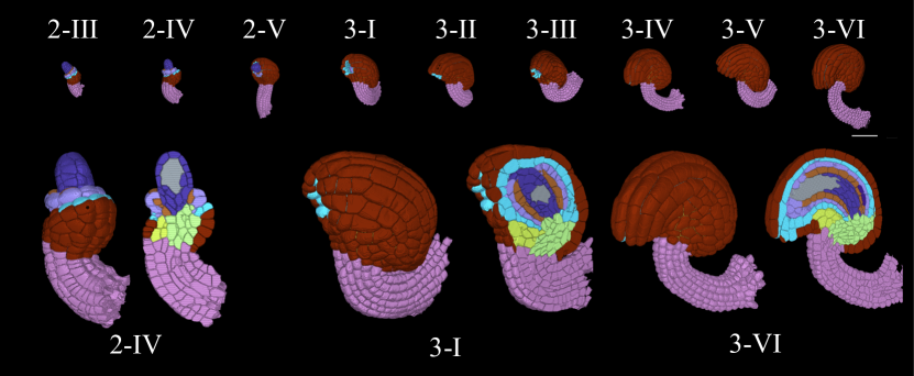
Figure 1: 3D surface view of a small subset of specimens from the CellTypeGraph Benchmark. Different developmental stages are indicated. From left to right the tissue complexity increases with organ growth. Scale bar $50\mu m$. Bottom: three stages are represented with their 3D view and a 2D section displaying the internal tissue architecture. Colors show ground truth cell types.

2.1 Overview

We introduce the CellTypeGraph Benchmark, aiming to give a valuable tool to the geometric learning community. To do so, we distilled a publicly available biological dataset [53] into a ready-to-use machine learning benchmark. In particular, we would like to focus the community’s attention on two primary objectives:

• Finding better graph neural network architectures and methodologies. In this case, we encourage using our pre-computed features, thus allowing direct comparison with our baseline, see Sec. 4.

• Finding more expressive features or, alternatively, replace hand crafted features by end-to-end learning. We will expand on this point in Sec. 3.2.

Progressing in either of the two challenges is an equally valid contribution to achieving the final goal of improving automated tools for plant-biology.

The statistics of the dataset are summarized in Tab. 1.

2.2 Raw data

The benchmark dataset is obtained from 3D confocal microscopic images of Arabidopsis ovule [53]. Ovules are the female gametophyte in higher plants that eventually gives rise to seeds upon successful fertilization.

The 3D digital ovule atlas is a composite of raw cell boundary images and their respective cell segmentation which are further tissue annotated. Fig. 1 shows a sample ovule from each developmental stage. Ovules at early stages (2-III to 2-V) protrude from the placental surface as a simple three layered dome like structure. Ovules form a complex 3D tissue structure during integument initiation and outgrowth. Four layers of integument tissues surround the core of the organ (cell labels L1 to L4). Integument tissues undergo growth conflicts that result in their final shape with a hood-like outer structure at maturity. Inner tissue layers of integuments are arranged as a bent tube like shape. Overall, the organ is moulded by complex arrangements of cells in 3D that partly follow a stratified arrangement of cells in the medial and upper half of the organ and it also forms a partial radial and bilateral symmetry.

The ground truth cell type labels for the benchmark dataset were obtained semi-automatically by first using a modified detect layer stack process in MorphographX [48]; and then proofreading the results from these predictions manually. Essentially, the layered cells in the upper medial half of the organ were labeled by the cell layer detection method and then manually corrected, while the rest of the cells from the organ were labeled manually. This required extensive human input, totaling in the order of 60 human hours for the dataset in this study.

Tissue annotations allowed in extensive biological analysis of the cellular basis of growth in different tissues and at different developmental stages [53].

Pre-processing:

The segmentation images as published in [53] have been further manually curated. We have ensured that for each specimen, cells form a single connected component. In case of multiple specimen imaged together, they have been split in separate stacks. Lastly, cell type annotations have been added for missing cells. Although we did our best to hand curate the data, minor imperfections might still be present due to the variability of the organs. Since the L5 cell type is rarely present in the later stages, we slightly simplified the benchmark task by merging the cell types L4 and L5.

Number of specimens	84
Number of developmental stages	9
Total number of cells/nodes	95757
Total number of edges	632443
Average number of nodes per specimen	1140
Average number of edges per specimen	7529
Number of semantic classes	9
Number of node features	78
Number of edge features	11

Table 1: Salient statistics of the CellTypeGraph benchmark.

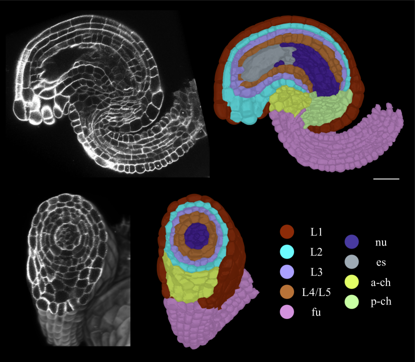
Figure 2: 2D section view of a mature Arabidopsis ovule displaying the raw cell boundary image and the respective CellTypeGraph ground truth labels manually annotated for the benchmark dataset. Different colors indicate different tissue labels annotated to the 3D instance cell segmentation. Abbreviations es: embryo sac, nu: nucellus, L1: outer layer of outer integument, L2: inner layer of outer integument, L3: outer layer of inner integument, L4/L5: inner layer of inner integument, fu: funiculus, a-ch: anterior chalaza, p-ch: posterior chalaza. Scale bar $20\mu m$.

2.3 Evaluation

Metrics:

The ovules cell types are imbalanced. This not only impacts the learning procedure but also requires attention when discussing the results quantitatively. An effective way to account for imbalance is to evaluate the model performance for each class independently and then report as final score the average of the single class results. In this work, we use two metrics, the simple global top-1 accuracy and the class-average accuracy.

In order to further stabilize the class-average accuracy, we ignored cell label $7$, see Fig. 2. Cell label $7$ represents the “embryo sac”. This tissue is not a cell in itself but is an ensemble of non-segmentable cells in the inner part of later-stage ovules. This region is unique and distinct, being the largest and highest degree node in the cell graph. Nevertheless, we kept the “embryo sac” in the benchmark for training purposes because of its crucial role in graph connectivity.

Moreover, if any cell type is not present in a specific specimen, that cell type will not be counted in the class-average accuracy, i.e.,

$$\textit{class-average accuracy}=\frac{1}{N_{s}}\sum_{s=1}^{N_{s}}\frac{\sum_{c}a_{c}\cdot\mathbbm{1}_{s,c}}{\sum_{c}\mathbbm{1}_{s,c}}$$

where $N_{s}$ is the number of specimens, $a_{c}$ is the one-vs-all class accuracy, $\mathbbm{1}$ is an indicator function valued $1$ if the class $c$ is present in the specimen $s$, 0 otherwise. This is particularly relevant in the early stages of development.

We release evaluation code for all the metrics introduced above bundled with our benchmark.

Experts consensus

The cell types are identified based on patterns of gene expression, cell position in space, and context in terms of tissue layers. The consensus is strong for layered cell types (L1 to L4); here, segmentation quality is the dominant source of ambiguity. But variability can arise in regions where the boundaries of the tissue groups are hard to determine from the cell position itself; for example, the boundary between fu, ch, and nu. In order to assess this variability quantitatively and assess a reference performance for an expert biologist, we produced an independent second set of labels. The overall results are reported in Tab. 2, while an additional breakdown of expert performance at different developmental stages and for different classes is reported in Appendix E.

Training and evaluation splits:

We release our CellTypeGraph data loader in two different modes: a standardized train-validation-test split, and a five fold cross-validation split.

Although train-validation-test splits are standard practice in popular machine learning benchmarks, this approach makes evaluations susceptible to sampling biases [44]. In our CellTypeGraph, we have high variability between specimens both intra-stage and inter-stage, see Fig. 1. This, combined with the relatively small number of specimens, makes the splits highly susceptible to sampling bias. We address the stage variability by sampling the same number of specimen from each stage.

However, to further unbias our experiments, we preferred to focus on a five-fold cross-validation approach. Cross-validation mitigates the noise coming from the random sampling at the expense of a more costly training. All presented experiments have been evaluated using cross-validation.

3 Features

This section details the node and edge features included in the CellTypeGraph benchmark. However, before motivating their choice, it is necessary to discuss the reference system used to express position and orientation dependent features.

3.1 Reference systems

Global reference system:

Ovule images acquired by the microscope are not always oriented in the same direction. This inconsistency in specimen orientation could cause poor generalization of trained models. Possible solutions are to systematically use rotation and translation equivariant methods or to fix a landmark-based global reference system. The first solution is more general and shows great potential in terms of generalization and parameter efficiency [12, 22, 40]. Equivaraint methods have a clear advatage when no standardized orientation can be formed, as in general chemical problems. In our case, an unambiguous standard pose can be defined and so for simplicity we opt for a landmark-based approach.

More specifically, we evaluate four landmark-based approaches, both supervised (Label Surf, Label Fu) and unsupervised (ES trivial, ES PCA). Detailed descriptions can be found in Appendix A. All coordinate systems yield similar accuracy, see Sec. 4.2. Nevertheless, the local reference Label Surf is slightly more consistent and less prone to outliers compared with the others, see Fig. 3. Hence Label Surf was used as default orientation system for all of our experiments.

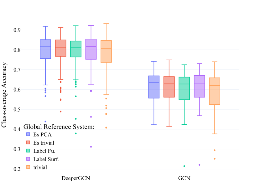
Figure 3: All reference systems are equally good. We trained both GCN and DeeperGCN on five distinct reference systems. There is no statistically significant difference in using either reference system. The only difference we could observe was in the spread of outliers.

Local reference system:

Ovule cells have no distinctive anisotropy that can be used to define a local orientation. However, preferential direction of growth and divisions along the central curved axis of the organ result in filar arrangement of cells within integument tissue layers (L1 to L4). This regular filar arrangement of cells can be used to identify integument tissues and separate them from one another. Integument tissues divide anticlinally to maintain their sheet like structure. Cell divisions happen mainly along the transverse anticlinal direction allowing the tissue to grow in length. Division planes can be further mapped to faces of cell wall extracted from a 3D instance cell segmentation. This includes longitudinal anticlinal wall, transverse anticlinal wall and periclinal wall. In order to exploit this prior, we construct a heuristic algorithm to identify transverse anticlinal walls and define a growth axis based on their connectivity.

Moreover, these tissues (L1 to L4), follow a stratified pattern as they continue dividing anticlinally. In this case, we propose another simple heuristic to construct a surface axis, parallel to the stratification direction. Both algorithms are described in details in Appendix B. The approximate growth axis and surface axis we find in this way have two significant limitation: the axes are not guaranteed to be orthogonal, and only their orientation is defined, but not their direction. Lastly, in order to have a complete 3D basis for our local reference system, we simply compute a third axis orthogonal to the first two. An illustration of the predicted growth and surface axes can be found in Fig. 4.

Figure 4: Automatically extracted local orientation features: the growth and surface directions are represented by the solid yellow lines and solid red lines respectively. Left: a 3D surface view of a mature Arabidopsis ovule overlaid with the predicted growth directions. The axis predictions align well with the filar arrangement of cells on the organ surface. Right: surface and growth orientations from the same ovule. Although the orientation of the growth axis follows the regular structure of the organ, the direction of the axis is arbitrary.

3.2 Feature extraction

As a first step, we compute the Cell Adjacency Graph $G\left(\mathcal{N},\mathcal{E}\right)$, where every cell is represented as node $n_{i}\in\mathcal{N}$ and an edge $e_{i,j}\in\mathcal{E}$ connects every pair of touching cells. Secondly, we sample a fixed number of points from the surface of each cell. To obtain equally distributed points, we use the farthest points sampling algorithm [36] over the cell surfaces. These sampled points are used to compute downstream features more efficiently, when necessary. However, the same surface samples could potentially be used to learn features end-to-end, using ideas from equivariant point cloud architectures. Although this direction is enticing, it would result in a much more complex pipeline. We also sample points from the boundary shared by any two touching cells, using the same sampling strategy. In each case, we sample 500 points per node/per edge.

We can divide all features into two categories: invariant and covariant features.

Invariant features

are independent from the reference system, and do not change under rotation or translation of the specimen. These features are either morphological — such as the cell volume, surface area, lengths along the local reference axis, and the angle formed between the surface and growth axis — or they are derived from the Cell Adjacency Graph, such as the shortest path from each node to the ovule surface, current-flow closeness centrality [47], and degree centrality.

Covariant features

instead transform with the reference system under rotation and translation. In this category we include: the cell center of mass, the local reference axes, and the cell PCA axes. In addition we also include: the angles formed between the local and the global reference system, and the angles between PCA axes and the global reference system. Although angles are not formally covariant, they are derived from covariant features and transform predictably under rotation and translation.

Edge features

are also pre-computed in our benchmark, in particular: shared cell boundary surface, the distance between adjacent centers of mass, and the angles between the local reference axes of adjacent cells. But as discussed in Sec. 4.1, these brought no significant improvement in the architectures we tested.

3.3 Feature homogenization

Appropriate feature processing has a great impact on the training dynamics. It is extremely important to properly normalize and homogenize incommensurable features before concatenating them.

To provide the orientation of PCA and local reference system axes to the network, we used the following transformation:

$$f:\mathbb{R}^{3}\rightarrow\mathbb{R}^{6},\left(x,y,z\right)\rightarrow\left(x^{2},y^{2},z^{2},xy,xz,yz\right),$$

That is, we removed the ambiguity in choosing direction and not just orientation. This yields an embedding of the manifold of orientations ${\mathbb{R}P}^{2}$ in $\mathbb{R}^{6}$, whose existence is guaranteed by the Whitney embedding theorem [55, 1].

All scalar features (except angles) are normalized to zero mean and unit variance. Furthermore, we encode categorical features as a one-hot vector and scale vector features to unit norm.

This protocol has been established by testing different preprocessing and normalization strategies for each group of features. Results are shown in Appendix C.

We made a best effort to ensure that the features we selected are expressive. However, our data loader can be easily extended to add new features or change the processing of the current features. The features discussed so far are all included in the loader by default, but in Appendix C we list additional features. All raw segmentations, annotations and pre-computed features are available at https://zenodo.org/record/6374104.

4 Benchmarking graph neural networks

To show the accuracy of existing methods on this new benchmark, we experiment with a large variety of models. We tried to represent the most prevalent graph neural networks paradigms. In particular, we tested graph convolutional networks, attention or transformer based architectures as well as message-passing based architectures.

Architectures:

We tested the following graph neural network architectures: GCN [25], GraphSAGE, [18], GIN [59], GCNII [7], and DeeperGCN [27, 28]; all as implemented in [11]. Moreover, we tested a two layer re-implementation of the graph attention network GAT [52] architecture, a variation of the same architecture GATv2 using the graph convolution operation introduced in [5], and a further variation TransformerGCN utilizing a transformer [51] based graph convolution from [45].

Two of the architectures tested can take into account edge features, the TransformerGCN and the DeeperGCN. When trained with edge features we will refer to them as EdgeTransformerGCN and EdgeDeeperGCN. All models used softmax as last layer activation.

Training:

All models have been trained with the ADAM optimizer [23] and cross entropy loss with $\mathbbm{L}_{2}$ weight penalty. Learning rate, weight regularization and model specific hyperparameters such as: number of layers, hidden features, dropout etc. have been tuned for each model using a coarse grid search.

Every training instance uses a single GPU and less than 2GB of VRAM. A complete five fold cross validation of the DeeperGCN completes in under one hour using a single Nvidia RTX6000 GPU. For all experiments, source code is provided at https://github.com/hci-unihd/plant-celltype.

Model
Node Classification	top-1 acc.	class-avg. acc.
GIN [59]	$0.714\pm 0.071$	$0.563\pm 0.136$
GCN [25]	$0.762\pm 0.043$	$0.617\pm 0.077$
GAT [52]	$0.824\pm 0.033$	$0.705\pm 0.084$
GATv2 [5]	$0.855\pm 0.041$	$0.757\pm 0.087$
GraphSAGE [18]	$0.859\pm 0.048$	$0.765\pm 0.093$
GCNII [7]	$0.863\pm 0.050$	$0.772\pm 0.100$
Transf. GCN [45]	$0.868\pm 0.045$	$0.779\pm 0.098$
EdgeTransf. GCN [45]	$0.868\pm 0.044$	$0.777\pm 0.098$
DeeperGCN [28]	$\textbf{0.877}\pm\textbf{0.050}$	$\textbf{0.796}\pm\textbf{0.098}$
EdgeDeeperGCN [28]	$\textbf{0.878}\pm\textbf{0.047}$	$\textbf{0.797}\pm\textbf{0.095}$
Expert Biologist	$0.932\pm 0.025$	$0.909\pm 0.049$

Table 2: Top-1 accuracy and class-average accuracy obtained by different architecture on the node classification task. DeeperGCN is consistently the best performing architecture. Nevertheless, DeeperGCN results are still weaker than human expert. EdgeDeeperGCN and EdgeTransformerGCN have been trained with additional edge features, but their impact on our metrics was not significant. Uncertainty is defined as the standard deviation over all specimens and cross-validation folds.

4.1 Baseline results

In Tab. 2, we present the best performing models over the five-fold cross-validation splits according to the class-average accuracy. DeeperGCN is consistently the best performing architecture, although it does not match yet the expert biologist performance.

Overall, all attention mechanism methods performed relatively well, while simpler models like GCN and GIN struggled the most. For both high- and low-end models, using edge features did not increase accuracy. Fig. 6 shows the class-average accuracy broken down by developmental stages. While DeeperGCN has a decisive advantage in the later stages compared to GCN, we can observe a much narrower spread in the early stages (2-III to 2-V). Fig. 5 shows the average accuracy by cell type. One can easily identify the categories L2, L4 and ac to be the most challenging for both GCN and DeeperGCN.

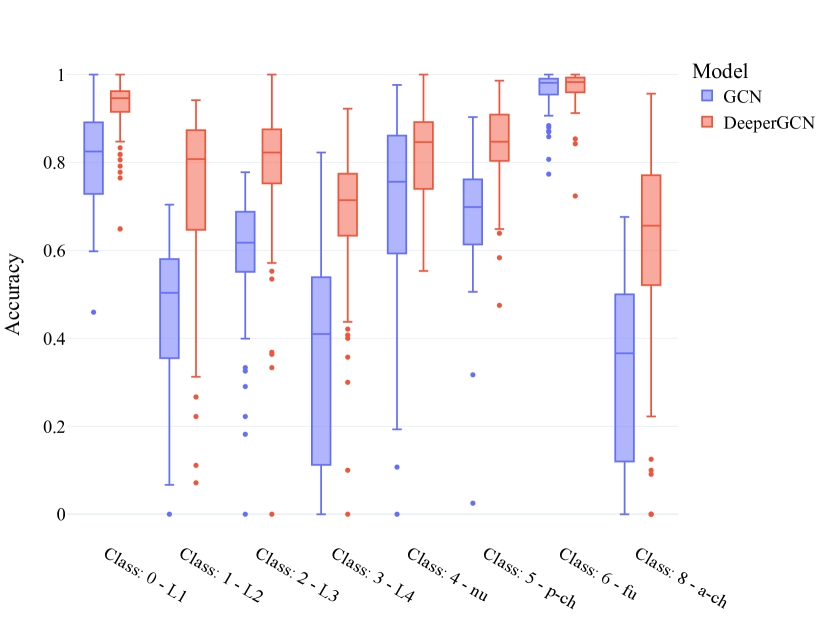
Figure 5: Top-1 accuracy divided by ground truth category. Accuracy varies drastically across classes. In particular, the GCN accuracy plummets for L2, L4, and a-ch tissues.

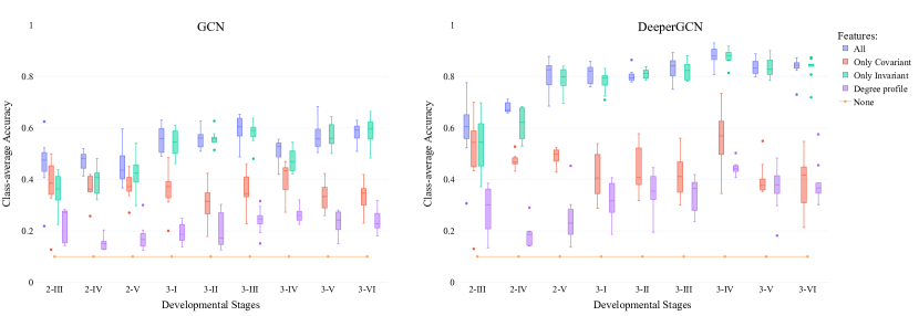
Figure 6: Comparison of the class average accuracy for four different feature sets. As one would expect, using all features consistently achieves the highest accuracy. Interestingly, one can observe that the covariant features mostly contribute to accuracy in the early stages (2-III to 2-V). In the later stages (3-I to 3-VI), the invariant features are the major contributors to the overall accuracy. Lastly, even when using only the local degree profile of a node as its feature, the networks are still able to make better than random predictions on the task.

4.2 Additional experiments

The same standardized setup was used for all our additional experiments. We limited ourselves to two models, the GCN [25] and the DeeperGCN [28], and used optimal hyper-parameters from Sec. 4, see Appendix D for each.

4.2.1 Importance of the global reference system

As discussed in Sec. 3.1, some of the features are sensitive to the orientation of the specimen. We tested and compared four landmark-based orientations plus the trivial orientation, i.e., center of mass in the origin and original orientation as acquired by the microscope. From Fig. 3 we can observe no significant difference between different orientations. The only relevant difference is that the reference system found using the labels exhibits an overall smaller variance across specimens. On the other end, the trivial representation manifests the most significant number of outliers. Another interesting question for practitioners is the ability to generalize if the reference system changes. We tested that by training our pipeline with three different orientations and always testing on the same. As shown in Tab. 4, at test time, there is a significant drop in accuracy when evaluating on a different orientation. However, the experiment also shows that this can be mitigated by training on multiple orientations at the same time.

4.2.2 Invariant vs covariant features

To evaluate the respective contribution of invariant and covariant features to the accuracy, we trained our models using solely one of the two. Tab. 3 shows that the invariant features are unquestionably what the neural networks rely on most.

To further understand the difference, in Fig. 6 we report our results for each development stage separately. One can see a distinction between the two feature groups: the invariant features have a stronger impact on the accuracy in the later stages (3-I to 3-VI), while the covariant features have a more prominent role in the early stages (2-III to 2-V).

4.2.3 Local graph features alone

To emphasize the importance of the Cell Adjacency Graph structure for solving this task, we also trained models using only the degree of a node and distribution of degrees of is neighbours, the so called degree profile [6]. This is an extremely unfavorable setup since the degrees are quite homogeneous across the ovule cell graph. The results, shown in Fig. 6, reveal that even then, the networks are still able to predict systematically better than chance. Moreover, DeeperGCN in later stages performed comparably to the same model trained using the covariant features.

Features	GCN	DeeperGCN
	$\Delta$ class-avg. acc.	$\Delta$ class-avg. acc.
Only invariant	$-0.028$	$-0.019$
Only covariant	$-0.175$	$-0.337$

Table 3: Contribution of each feature group to the accuracy. The table shows the difference between the class average accuracy of the baseline model and the class average accuracy of the perturbed model. The lower the delta, the higher is the feature importance for the neural networks. For both architectures, the invariant features are substantially more important than the covariant features.

Training Data	GCN	DeeperGCN
	class-avg. acc.	class-avg. acc.
ES PCA	$0.578\pm 0.089$	$0.754\pm 0.118$
All but Label Surf	$0.618\pm 0.086$	$0.787\pm 0.103$
Label Surf	$0.613\pm 0.080$	$0.790\pm 0.100$

Table 4: Generalization under different orientations. We tested how robust our baseline is to changes in the global orientation axes. We trained our model in different orientations, and we tested it on a particular one, Label Surf. From the class average accuracy, we can observe a substantial accuracy drop when training on a single different reference system, ES PCA. However, this can be easily compensated by augmenting the training data with multiple orientations. Uncertainty is defined as the standard deviation over all specimens.

5 Limitations

The CellTypeGraph Benchmark is limited by the number of specimen. Imaging, segmenting, and annotating large 3D volumes is very time-consuming, and thus the number of specimens available is smaller compared to other datasets [58, 17]. This limitation can be mitigated by data augmentation. Although not exhaustive, this route did not show visible improvements in our experiments. A description of the experiments performed and results can be found in Appendix F.

Nevertheless, the structural complexity of the ovules makes them a perfect candidate for a benchmark. However, ovules are not a universal proxy for all organs in plant-biology, thus pre-trained models on our benchmark are likely to fail on different organs. Possible solutions are: i) retraining the models when labels are available. ii) Using self-supervised methods such as graph autoencoders [24, 39] followed by community clustering in latent space. Such a setup has proven successful in single-cell data analysis [3, 30]. iii) Speeding up semi-automated labeling by employing active learning.

In the benchmark, the two main sources of complexity are the hand-crafted features and the need to define a global orientation. End-to-end feature learning could be achieved by applying models from the point clouds geometric deep learning domain [35, 36, 29] to our surface sample, see Sec. 3.2. Moreover, new exciting frameworks like [13] are expediting easy access to equivariant neural network architectures.

6 Acknowledgments

This work was supported by the Deutsche Forschungsgemeinschaft (DFG) research unit FOR2581 Quantitative Plant Morphodynamics.

7 Conclusion

We have introduced a new graph benchmark for node classification, extensively tested several relevant graph neural networks architectures, and released tools for quick experimentation, data handling, and evaluation.

Although results from our baseline are encouraging, we are excited to discover how far the community will push this task. As discussed in Sec. 5, tissue labeling in 3D virtual organs is a relevant and relatively unexplored domain. We also hope to see use of the benchmark outside the strict paradigms of supervised learning, such as self-supervised and active learning.

Appendix A Global reference axis

Our landmark-based global reference systems are defined by fixing an origin and an orthogonal 3D vectors basis. A good land-mark should be retrievable from the ground truth labels at training time, but should also be easy to identify by a human without ground truth labels at test time.

We choose the following four approaches:

Label Surf:

The origin is defined as the center of mass of the L1 tissue. The main axis is found by approximately determining the integument tissue symmetry axis. This is achieved by finding for each tissue in the integument (L2, L3, L4, es, nu) the respective center of mass. Then, we use least-square linear regression to find the best line interpolating the integument tissue. The second axis is found by finding the line passing through fu tissue center of mass and perpendicular to the main axis. The third axis is computed by taking the cross-product between the first and second axes.

Label Fu:

The origin is defined as the center of mass of the fu tissue. The global axes are computed as in the Label Surf.

Es trivial:

Here we use the Es tissue to fix an origin for the reference system. It is usually easily identifiable by its large size and central position. We set the reference system origin to the Es center of mass. While for the axis, we use the original orientation as acquired by the microscope.

Es PCA:

The origin is the same as Es Trivial. But the system axes are set to the PCA axes of the whole ovule.

Our python implementation can be found at: https://github.com/hci-unihd/plant-celltype/blob/main/plantcelltype/features/cell_vector_features.py.

Appendix B Growth and surface axis

To compute the local reference system, we designed two simple heuristics. We estimate the surface axis of a cell by averaging over directions corresponding to the edges connecting the cell to all neighbors which are closer to the surface. These directions are defined as the edge surface normal direction.
The growth axes are found by looking for each cell the most co-linear pair of neighboring cells.

The algorithms used to compute the surface axis and growth axis are described in more detail respectively in Algorithm 1 and Algorithm 2. Our python implementation can be found at: https://github.com/hci-unihd/plant-celltype/blob/main/plantcelltype/utils/axis_transforms.py.

node, edges $\triangleright$ Vectors containing: nodes ids, edges ids.

hops $\triangleright$ Vectors containing: number of hops from each node to the surface.

directions, bg $\triangleright$ Vector containing: edges directions (surface normal), background node id.

N $\leftarrow$ len(node)

surface-axis $\leftarrow$ zeros(N, 3) $\triangleright$ Initialize an array full of zeros.

for ($i=0$, $i=\text{N}$, $i$++) do

     if $\text{hops}_{i}=1$ then $\triangleright$ I.e. node is on the organ surface.

         e $\leftarrow$ find-edge($\text{node}_{i}$, bg, edges) $\triangleright$ Find edge id between $\text{node}_{i}$/$\text{node}_{j}$.

         $\text{surface-axis}_{i}\leftarrow\text{directions}_{e}$

     else

         $\text{neighbors}_{i}\leftarrow$ find-neighbors($\text{node}_{i}$, edges) $\triangleright$ Find all nodes neighbors of $\text{node}_{i}$.

         $\text{N}_{i},\text{count}\leftarrow$ $\textit{len}(\text{neighbors}_{i}),0$

         for $j=0$, $j=\text{N}_{i}$, $j$++ do $\triangleright$ Loop over the neighborhood.

              if $\text{hops}_{j}<\text{hops}_{i}$ then $\triangleright$ If neighbor is closer to surface.

                  e $\leftarrow$ find-edge($\text{node}_{i}$, $\text{node}_{j}$, edges) $\triangleright$ Find edge id between $\text{node}_{i}$/$\text{node}_{j}$.

                  $\text{surface-axis}_{i}\leftarrow\text{surface-axis}_{i}+\text{directions}_{e}$ $\triangleright$ Average edges normal.

                  count = count + 1

              end if

              $\text{surface-axis}_{i}\leftarrow\text{surface-axis}_{i}/\text{count}$

         end for

     end if

end for

Algorithm 1 Compute Surface Axis

node, edges $\triangleright$ Vectors containing: nodes ids, edges ids.

coms, hops $\triangleright$ Vectors containing: nodes center of mass, number of hops from each node to the surface.

N $\leftarrow$ len(node)

growth-axis $\leftarrow$ zeros(N, 3) $\triangleright$ Initialize an array full of zeros.

for ($i=0$, $i=\text{N}$, $i$++) do

     $\Theta_{min}\leftarrow$ 1

     $\text{neighbors}_{i}\leftarrow$ find-neighbors($\text{node}_{i}$, edges) $\triangleright$ Find all nodes neighbors of $\text{node}_{i}$.

     $\text{N}_{i}\leftarrow$ $\textit{len}(\text{neighbors}_{i})$

     for $j=0$, $j=\text{N}_{i}$, $j$++ do $\triangleright$ Loop over all tuple ($\text{node}_{j}$, $\text{node}_{j}$) of distinct neighbors of $\text{node}_{i}$.

         $\text{vector}_{ij}$ = get-vector($\text{node}_{i}$, $\text{node}_{j}$, coms) $\triangleright$ Find vector connecting $\text{node}_{i}$/$\text{node}_{j}$ center of masses.

         for $k=j+1$, $k=\text{N}_{i}$, $k$++ do

              $\text{vector}_{ik}$ = get-vector($\text{node}_{i}$, $\text{node}_{k}$, coms)

              $\Theta$ = get-angle($\text{vector}_{ij}$, $\text{vector}_{ik}$) $\triangleright$ Angle is measured as the normalized dot product between the two vectors.

              if $\Theta<\Theta_{min}$ and $\text{hops}_{i}=\text{hops}_{j}=\text{hops}_{k}$ then $\triangleright$ When the angle is minimum the cell are the most co-linear.

                  $\Theta_{min}\leftarrow\Theta$

                  $\text{growth-axis}_{i}\leftarrow\text{vector}_{ij}$

              end if

         end for

     end for

end for

Algorithm 2 Compute Growth Axis

Appendix C Features

We here report the results of additional experiments conducted to identify the best feature homogenization strategy. In Fig. 7, we tested the difference between different vector representations. In Fig. 9 and Fig. 8, we tested the normalizations for the graph features and the maximum value to be used in our hops to surface feature. In Fig. 10 and Fig. 11 we tested different normalization applied to respectively morphological and angles features. Lastly, in Fig. 12 we tested the impact of using lengths measured in several directions as features, similarly to [41]. An overview of all features available in the CellTypeGraph benchmark is reported in Tab. 5, Tab. 6. Our python implementation can be found at: https://github.com/hci-unihd/plant-celltype/tree/main/plantcelltype/features

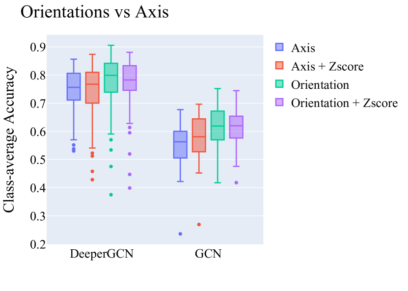
Figure 7: Class-average accuracy comparison between different vector features representations. Using the orientation instead of axis resulted in a small but consistent improvement in performance.

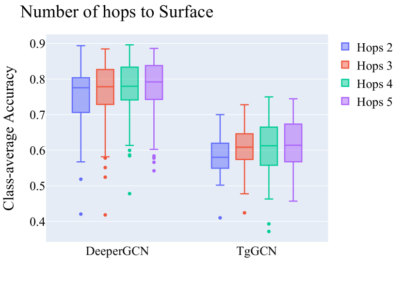
Figure 8: Class-average accuracy with varying maximum number of hops. Hops to surface are intuitively closely related to the tissue stratification L1-L4, but their relation loosen with depth. We tested how important this feature is by clipping its value. From the results one can see that the feature contribution saturates after three hops.

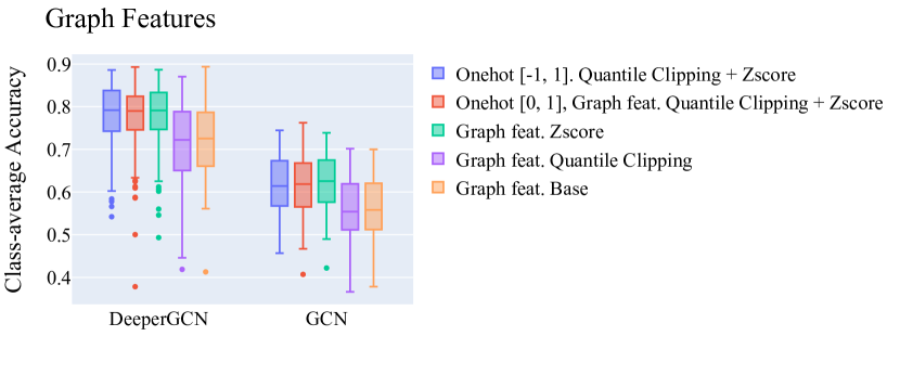
Figure 9: Class-average accuracy between different graph feature normalizations. One can see a slight accuracy improvement using z-score normalization.

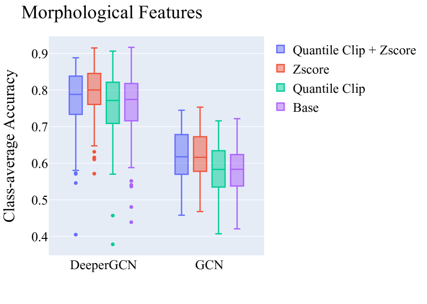
Figure 10: Class-average accuracy comparison between different morphological features normalizations. One can see a slight accuracy improvement using z-score normalization.

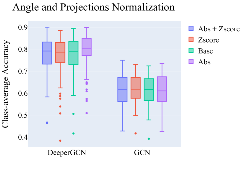
Figure 11: Class-average accuracy between different angles normalization. Angles are naturally normalized between -1 and 1, in our experiments the z-score had no significant impact.

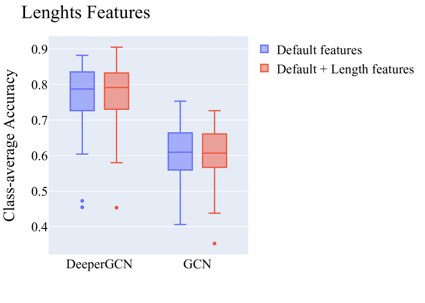
Figure 12: Class-average accuracy between: baseline features only, and baseline features plus additional lengths features. In our experiments the additional lengths showed no significant contribution to the accuracy.

Feature Name	Invariant	Default	Size	Description
Center of mass		✓	3	Cell center of mass represented in the global reference system, expressed in $\mu m$.
Center of mass / GRS Proj.			3	Angles between the cell center of mass and the global reference system.
LRS axis			9	Growth axis, surface axis and third perpendicular axis.
LRS orientations		✓	18	Direction invariant growth axis, surface axis and third perpendicular axis.
LRS / GRS Proj.	✓	✓	9	Angles between the LRS axis and the global reference system.
Growth/Surface axis angle	✓	✓	1	Angle between growth and surface axis.
Growth axis alignment	✓	✓	1	Angle between periclinial cell walls along predicted growth direction, measure how good is the fit is.
Length LRS	✓	✓	3	Cell length along the LRS directions.
PCA axis			9	Principal component analysis axis.
PCA orientations		✓	18	Direction invariant principal component analysis.
PCA / GRS Proj.	✓	✓	9	Angles between the PCA axis and the global reference system.
PCA explained variance	✓	✓	3	PCA axis explained variance.
Surface	✓	✓	1	Cell surface area in $\mu m$.
Volume	✓	✓	1	Cell volume in $\mu m$.
Lengths uniform samples			64	Cell length in uniform directions.
Hops to Surface	✓	✓	1	Shortest path length on the graph between a cell and the surface. For this measure we ignore the geo-localization of nodes, and consider all neighbors one hop distant.
Degree Centrality	✓	✓	1	Degree centrality.
CFC centrality	✓	✓	1	Current-flow closeness centrality.

Table 5: Complete list of node features pre-computed in the CellTypeGraph.

Feature Name	Invariant	Default	Size	Description
Center of mass surface	✓	✓	3	Cell Surface (edge) center of mass represented in the global reference system, expressed in $\mu m$.
Center of mass distance	✓	✓	1	Distance between two adjacent cell center of mass.
Center of mass /GRS Proj.		✓	3	Angles between two adjacent cell center of mass direction and the global reference system.
LRS Proj.	✓	✓	3	Angles between local reference system in adjacent cells.
Surface	✓	✓	1	Edge surface area in $\mu m$.

Table 6: Complete list of edge features pre-computed in the CellTypeGraph.

Appendix D Grid search complete results

Experiment parameters setup is reported in Tab. 7. The configuration files used to run our experiments can be fount at: https://github.com/hci-unihd/plant-celltype/tree/main/experiments/node_grid_search

Model	Optimizer	Model Params.	top-1 acc.	class-avg. acc.
GIN [59]	lr $=10^{-2}$	# feat $=64$	$0.714\pm 0.071$	$0.563\pm 0.136$
	wd $=10^{-5}$	# layers $=2$
		dropout $=0.1$
GCN [25]	lr $=10^{-2}$	# feat $=128$	$0.762\pm 0.043$	$0.617\pm 0.077$
	wd $=10^{-5}$	# layers $=2$
		dropout $=0.5$
GAT [52]	lr $=10^{-3}$	# feat $=256$	$0.824\pm 0.033$	$0.705\pm 0.084$
	wd $=0$	# layers $=2$
		dropout $=0.5$
		heads $=3$
		concat. $=$ True
GATv2 [5]	lr $=10^{-3}$	# feat $=256$	$0.855\pm 0.041$	$0.757\pm 0.087$
	wd $=10^{-5}$	# layers $=2$
		dropout $=0.5$
		heads $=3$
		concat. $=$ True
GraphSAGE [18]	lr $=10^{-3}$	# feat $=128$	$0.859\pm 0.048$	$0.765\pm 0.093$
	wd $==10^{-5}$	# layers $=4$
		dropout $=0.1$
GCNII [18]	lr $=10^{-2}$	# feat $=128$	$0.863\pm 0.050$	$0.772\pm 0.100$
	wd $=10^{-5}$	# layers $=4$
		dropout $=0.0$
		share weight $=$ False
Transf. GCN [45]	lr $=10^{-3}$	# feat $=128$	$0.868\pm 0.045$	$0.779\pm 0.098$
	wd $=10^{-5}$	# layers $=2$
		dropout $=0.5$
		heads $=3$
		concat. $=$ True
EdgeTransf. GCN [45]	lr $=10^{-3}$	# feat $=128$	$0.868\pm 0.044$	$0.777\pm 0.098$
	wd $=0$	# layers $=2$
		dropout $=0.5$
		heads $=5$
		concat. $=$ True
DeeperGCN [28]	lr $=10^{-3}$	# feat $=128$	$\textbf{0.877}\pm\textbf{0.050}$	$\textbf{0.796}\pm\textbf{0.098}$
	wd $=0$	# layers $=32$
		dropout $=0.0$
EdgesDeeperGCN [28]	lr $=10^{-3}$	# feat $=128$	$\textbf{0.878}\pm\textbf{0.047}$	$\textbf{0.797}\pm\textbf{0.095}$
	wd $=10^{-5}$	# layers $=16$
		dropout $=0.0$

Table 7: Best performing optimizer and model parameters according to the class-avg. accuracy.

Appendix E Expert agreement

In order to highlights the most challenging aspect of our CellTypeGraph Benchmark, we here report further analysis of the expert biologist performance, see Fig. 13 and Fig. 14.

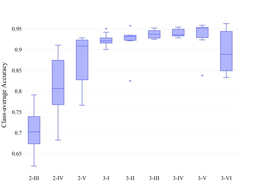
Figure 13: Class-average accuracy obtained by an expert biologist. The early stages pose the most substantial challenges, although the cause of such high variance can be attributed to the smaller number of cells for each specimen.

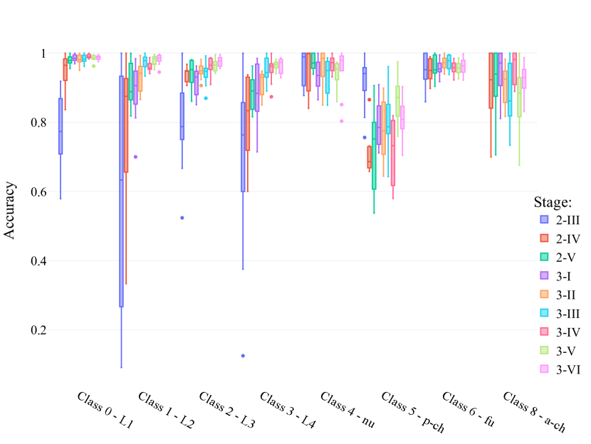
Figure 14: Per-class accuracy obtained by an expert biologist. In late stages the highest variability sources are the cell types p-ch and p-ch, while for early stages the highest variability is posed by the cell type L1 to L4.

Appendix F Data augmentation

Data augmentation is commonly used in machine learning to avoid overfitting in a small dataset and improve generalization. We tested the impact of two simple approaches on our CellTypeGraph Benchmark. The first augmentation is to add Gaussian distributed noise to the node features, while the second approach is to use random dropout of edges in the cell adjacency graph, results are reported in Fig. 15. Our preliminary results show a small effect of data augmentation on the metrics, but more exhaustive experimentation is necessary to draw more solid conclusions.

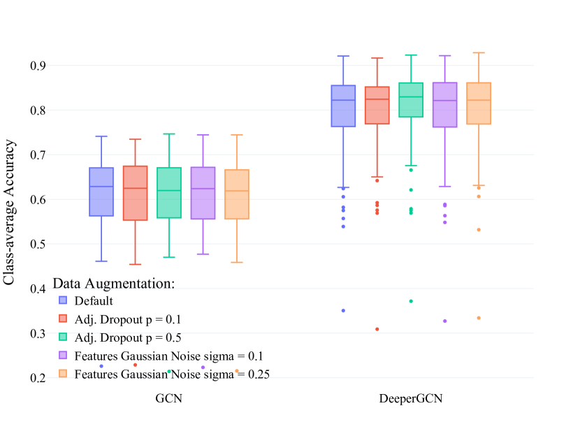
Figure 15: Comparison of the class-average accuracy for various combinations of network architecture, data augmentation technique, and parameters. The impact of data augmentation is negligible in all our experiments. Nevertheless, adjacency dropout (edge drop probability = 0.5) consistently improves accuracy for the DeeperGCN model.

Appendix G Baseline implementation details

In our baseline, we benchmark eight different graph neural network architectures. We report here the most salient implementation details. For GCN [25], GraphSAGE, [18], GIN [59], GCNII [7], and DeeperGCN [27, 28]; we followed the pytorch_geometric implementation [11]. In all the aforementioned architectures the convolutions block are composed as follows: Graph Convolution $\rightarrow$ Relu activation [2] $\rightarrow$ normalization $\rightarrow$ Dropout [46]. The number of convolutions blocks used is an hyper parameter. In addition in DeeperGCN and GCNII and addition linear layer is added before the first graph convolution layer and after the last graph convolution layer. While for the remaining architectures GAT [52], GATv2 [5], and TransformerGCN [51, 45], we used graph convolutions as implemented in [11] but with some minor differences in the convolution block layout: Graph Convolution $\rightarrow$ normalization $\rightarrow$ Relu activation [2] $\rightarrow$ Dropout [46]. All source implementation are released at https://github.com/hci-unihd/plant-celltype/blob/main/plantcelltype/graphnn/graph_models.py.

References

- [1] Masahisa Adachi. Embeddings and immersions. American Mathematical Soc., 2012.
- [2] Abien Fred Agarap. Deep learning using rectified linear units (relu). arXiv preprint arXiv:1803.08375, 2018.
- [3] Matthew Amodio, David Van Dijk, Krishnan Srinivasan, William S Chen, Hussein Mohsen, Kevin R Moon, Allison Campbell, Yujiao Zhao, Xiaomei Wang, Manjunatha Venkataswamy, et al. Exploring single-cell data with deep multitasking neural networks. Nature methods, 16(11):1139–1145, 2019.
- [4] Lorenz C Blum and Jean-Louis Reymond. 970 million druglike small molecules for virtual screening in the chemical universe database gdb-13. Journal of the American Chemical Society, 131(25):8732–8733, 2009.
- [5] Shaked Brody, Uri Alon, and Eran Yahav. How attentive are graph attention networks? arXiv preprint arXiv:2105.14491, 2021.
- [6] Chen Cai and Yusu Wang. A simple yet effective baseline for non-attributed graph classification. arXiv preprint arXiv:1811.03508, 2018.
- [7] Ming Chen, Zhewei Wei, Zengfeng Huang, Bolin Ding, and Yaliang Li. Simple and deep graph convolutional networks. In International Conference on Machine Learning, pages 1725–1735. PMLR, 2020.
- [8] Tomasz Danel, Przemysław Spurek, Jacek Tabor, Marek Śmieja, Łukasz Struski, Agnieszka Słowik, and Łukasz Maziarka. Spatial graph convolutional networks. In International Conference on Neural Information Processing, pages 668–675. Springer, 2020.
- [9] Pim De Haan, Maurice Weiler, Taco Cohen, and Max Welling. Gauge equivariant mesh cnns: Anisotropic convolutions on geometric graphs. In International Conference on Learning Representations, 2020.
- [10] Michaël Defferrard, Xavier Bresson, and Pierre Vandergheynst. Convolutional neural networks on graphs with fast localized spectral filtering. Advances in neural information processing systems, 29, 2016.
- [11] Matthias Fey and Jan E. Lenssen. Fast graph representation learning with PyTorch Geometric. In ICLR Workshop on Representation Learning on Graphs and Manifolds, 2019.
- [12] Marc Finzi, Samuel Stanton, Pavel Izmailov, and Andrew Gordon Wilson. Generalizing convolutional neural networks for equivariance to lie groups on arbitrary continuous data. In International Conference on Machine Learning, pages 3165–3176. PMLR, 2020.
- [13] Mario Geiger, Tess Smidt, Alby M., Benjamin Kurt Miller, Wouter Boomsma, Bradley Dice, Kostiantyn Lapchevskyi, Maurice Weiler, Michał Tyszkiewicz, Simon Batzner, Martin Uhrin, Jes Frellsen, Nuri Jung, Sophia Sanborn, Josh Rackers, and Michael Bailey. Euclidean neural networks: e3nn, 2020.
- [14] Robert Geirhos, Patricia Rubisch, Claudio Michaelis, Matthias Bethge, Felix A Wichmann, and Wieland Brendel. Imagenet-trained CNNs are biased towards texture; increasing shape bias improves accuracy and robustness. In International Conference on Learning Representations, 2018.
- [15] C Lee Giles, Kurt D Bollacker, and Steve Lawrence. Citeseer: An automatic citation indexing system. In Proceedings of the third ACM conference on Digital libraries, pages 89–98, 1998.
- [16] Justin Gilmer, Samuel S Schoenholz, Patrick F Riley, Oriol Vinyals, and George E Dahl. Neural message passing for quantum chemistry. In International conference on machine learning, pages 1263–1272. PMLR, 2017.
- [17] Rafael Gómez-Bombarelli, Jennifer N Wei, David Duvenaud, José Miguel Hernández-Lobato, Benjamín Sánchez-Lengeling, Dennis Sheberla, Jorge Aguilera-Iparraguirre, Timothy D Hirzel, Ryan P Adams, and Alán Aspuru-Guzik. Automatic chemical design using a data-driven continuous representation of molecules. ACS central science, 4(2):268–276, 2018.
- [18] William L Hamilton, Rex Ying, and Jure Leskovec. Inductive representation learning on large graphs. In Proceedings of the 31st International Conference on Neural Information Processing Systems, pages 1025–1035, 2017.
- [19] Mingguo He, Zhewei Wei, Hongteng Xu, et al. Bernnet: Learning arbitrary graph spectral filters via bernstein approximation. Advances in Neural Information Processing Systems, 34, 2021.
- [20] Lilan Hong, Mathilde Dumond, Mingyuan Zhu, Satoru Tsugawa, Chun-Biu Li, Arezki Boudaoud, Olivier Hamant, and Adrienne HK Roeder. Heterogeneity and robustness in plant morphogenesis: from cells to organs. Annual review of plant biology, 69:469–495, 2018.
- [21] Weihua Hu, Matthias Fey, Marinka Zitnik, Yuxiao Dong, Hongyu Ren, Bowen Liu, Michele Catasta, and Jure Leskovec. Open graph benchmark: Datasets for machine learning on graphs. Advances in neural information processing systems, 33:22118–22133, 2020.
- [22] Nicolas Keriven and Gabriel Peyré. Universal invariant and equivariant graph neural networks. Advances in Neural Information Processing Systems, 32:7092–7101, 2019.
- [23] Diederik P Kingma and Jimmy Ba. Adam: A method for stochastic optimization. In International Conference on Learning Representations, 2015.
- [24] Thomas N Kipf and Max Welling. Variational graph auto-encoders. arXiv preprint arXiv:1611.07308, 2016.
- [25] Thomas N Kipf and Max Welling. Semi-supervised classification with graph convolutional networks. International Conference on Learning Representations, 2017.
- [26] Hyunkwang Lee, Fabian M Troschel, Shahein Tajmir, Georg Fuchs, Julia Mario, Florian J Fintelmann, and Synho Do. Pixel-level deep segmentation: artificial intelligence quantifies muscle on computed tomography for body morphometric analysis. Journal of digital imaging, 30(4):487–498, 2017.
- [27] Guohao Li, Matthias Muller, Ali Thabet, and Bernard Ghanem. Deepgcns: Can GCNs go as deep as CNNs? In Proceedings of the IEEE/CVF International Conference on Computer Vision, pages 9267–9276, 2019.
- [28] Guohao Li, Chenxin Xiong, Ali Thabet, and Bernard Ghanem. Deepergcn: All you need to train deeper GCNs. arXiv preprint arXiv:2006.07739, 2020.
- [29] Yangyan Li, Rui Bu, Mingchao Sun, Wei Wu, Xinhan Di, and Baoquan Chen. PointCNN: Convolution on x-transformed points. Advances in neural information processing systems, 31:820–830, 2018.
- [30] Romain Lopez, Jeffrey Regier, Michael Cole, Michael Jordan, and Nir Yosef. A deep generative model for single-cell rna sequencing with application to detecting differentially expressed genes. arXiv preprint arXiv:1710.05086, 2017.
- [31] Andrew Kachites McCallum, Kamal Nigam, Jason Rennie, and Kristie Seymore. Automating the construction of internet portals with machine learning. Information Retrieval, 3(2):127–163, 2000.
- [32] Thomas Montenegro-Johnson, Soeren Strauss, Matthew DB Jackson, Liam Walker, Richard S Smith, and George W Bassel. 3DCellAtlas meristem: a tool for the global cellular annotation of shoot apical meristems. Plant methods, 15(1):1–9, 2019.
- [33] Thomas D Montenegro-Johnson, Petra Stamm, Soeren Strauss, Alexander T Topham, Michail Tsagris, Andrew TA Wood, Richard S Smith, and George W Bassel. Digital single-cell analysis of plant organ development using 3DCellAtlas. The Plant Cell, 27(4):1018–1033, 2015.
- [34] Adam Paszke, Sam Gross, Soumith Chintala, Gregory Chanan, Edward Yang, Zachary DeVito, Zeming Lin, Alban Desmaison, Luca Antiga, and Adam Lerer. Automatic differentiation in PyTorch. 2017.
- [35] Charles R Qi, Hao Su, Kaichun Mo, and Leonidas J Guibas. Pointnet: Deep learning on point sets for 3d classification and segmentation. In Proceedings of the IEEE conference on computer vision and pattern recognition, pages 652–660, 2017.
- [36] Charles Ruizhongtai Qi, Li Yi, Hao Su, and Leonidas J Guibas. PointNet++: Deep hierarchical feature learning on point sets in a metric space. Advances in Neural Information Processing Systems, 30, 2017.
- [37] Yassin Refahi, Argyris Zardilis, Gaël Michelin, Raymond Wightman, Bruno Leggio, Jonathan Legrand, Emmanuel Faure, Laetitia Vachez, Alessia Armezzani, Anne-Evodie Risson, et al. A multiscale analysis of early flower development in arabidopsis provides an integrated view of molecular regulation and growth control. Developmental Cell, 56(4):540–556, 2021.
- [38] Matthias Rupp, Alexandre Tkatchenko, Klaus-Robert Müller, and O Anatole Von Lilienfeld. Fast and accurate modeling of molecular atomization energies with machine learning. Physical review letters, 108(5):058301, 2012.
- [39] Amin Salehi and Hasan Davulcu. Graph attention auto-encoders. In 2020 IEEE 32nd International Conference on Tools with Artificial Intelligence (ICTAI), pages 989–996. IEEE, 2020.
- [40] Víctor Garcia Satorras, Emiel Hoogeboom, and Max Welling. E(n) equivariant graph neural networks. In Marina Meila and Tong Zhang, editors, Proceedings of the 38th International Conference on Machine Learning, volume 139 of Proceedings of Machine Learning Research, pages 9323–9332. PMLR, 18–24 Jul 2021.
- [41] Thorsten Schmidt, Taras Pasternak, Kun Liu, Thomas Blein, Dorothée Aubry-Hivet, Alexander Dovzhenko, Jasmin Duerr, William Teale, Franck A Ditengou, Hans Burkhardt, et al. The iRoCS Toolbox–3D analysis of the plant root apical meristem at cellular resolution. The Plant Journal, 77(5):806–814, 2014.
- [42] Kristof Schütt, Pieter-Jan Kindermans, Huziel Enoc Sauceda Felix, Stefan Chmiela, Alexandre Tkatchenko, and Klaus-Robert Müller. Schnet: A continuous-filter convolutional neural network for modeling quantum interactions. Advances in neural information processing systems, 30, 2017.
- [43] Prithviraj Sen, Galileo Namata, Mustafa Bilgic, Lise Getoor, Brian Galligher, and Tina Eliassi-Rad. Collective classification in network data. AI magazine, 29(3):93–93, 2008.
- [44] Oleksandr Shchur, Maximilian Mumme, Aleksandar Bojchevski, and Stephan Günnemann. Pitfalls of graph neural network evaluation. arXiv preprint arXiv:1811.05868, 2018.
- [45] Yunsheng Shi, Zhengjie Huang, Shikun Feng, Hui Zhong, Wenjing Wang, and Yu Sun. Masked label prediction: Unified message passing model for semi-supervised classification. In Proceedings of the Thirtieth International Joint Conference on Artificial Intelligence, IJCAI-21, 2021.
- [46] Nitish Srivastava, Geoffrey Hinton, Alex Krizhevsky, Ilya Sutskever, and Ruslan Salakhutdinov. Dropout: a simple way to prevent neural networks from overfitting. The journal of machine learning research, 15(1):1929–1958, 2014.
- [47] Karen Stephenson and Marvin Zelen. Rethinking centrality: Methods and examples. Social networks, 11(1):1–37, 1989.
- [48] Sören Strauss, Adam Runions, Brendan Lane, Dennis Eschweiler, Namrata Bajpai, Nicola Trozzi, Anne-Lise Routier-Kierzkowska, Saiko Yoshida, Sylvia Rodrigues da Silveira, Athul Vijayan, et al. MorphoGraphX 2.0: Providing context for biological image analysis with positional information. bioRxiv, 2021.
- [49] Hastie Trevor, Tibshirani Robert, and Jerome H Friedman. The elements of statistical learning: Data mining, inference, and prediction. Springer, 2017.
- [50] Oliver T Unke and Markus Meuwly. Physnet: A neural network for predicting energies, forces, dipole moments, and partial charges. Journal of chemical theory and computation, 15(6):3678–3693, 2019.
- [51] Ashish Vaswani, Noam Shazeer, Niki Parmar, Jakob Uszkoreit, Llion Jones, Aidan N Gomez, Łukasz Kaiser, and Illia Polosukhin. Attention is all you need. In Advances in neural information processing systems, pages 5998–6008, 2017.
- [52] Petar Veličković, Guillem Cucurull, Arantxa Casanova, Adriana Romero, Pietro Liò, and Yoshua Bengio. Graph attention networks. In International Conference on Learning Representations, 2018.
- [53] Athul Vijayan, Rachele Tofanelli, Sören Strauss, Lorenzo Cerrone, Adrian Wolny, Joanna Strohmeier, Anna Kreshuk, Fred A Hamprecht, Richard S Smith, and Kay Schneitz. A digital 3D reference atlas reveals cellular growth patterns shaping the arabidopsis ovule. Elife, 10:e63262, 2021.
- [54] Alexander D Weston, Panagiotis Korfiatis, Timothy L Kline, Kenneth A Philbrick, Petro Kostandy, Tomas Sakinis, Motokazu Sugimoto, Naoki Takahashi, and Bradley J Erickson. Automated abdominal segmentation of CT scans for body composition analysis using deep learning. Radiology, 290(3):669–679, 2019.
- [55] Hassler Whitney. The self-intersections of a smooth n-manifold in 2n-space. Annals of Mathematics, pages 220–246, 1944.
- [56] Lisa Willis, Yassin Refahi, Raymond Wightman, Benoit Landrein, José Teles, Kerwyn Casey Huang, Elliot M Meyerowitz, and Henrik Jönsson. Cell size and growth regulation in the arabidopsis thaliana apical stem cell niche. Proceedings of the National Academy of Sciences, 113(51):E8238–E8246, 2016.
- [57] Felix Wu, Amauri Souza, Tianyi Zhang, Christopher Fifty, Tao Yu, and Kilian Weinberger. Simplifying graph convolutional networks. In Kamalika Chaudhuri and Ruslan Salakhutdinov, editors, Proceedings of the 36th International Conference on Machine Learning, volume 97 of Proceedings of Machine Learning Research, pages 6861–6871. PMLR, 09–15 Jun 2019.
- [58] Zhenqin Wu, Bharath Ramsundar, Evan N Feinberg, Joseph Gomes, Caleb Geniesse, Aneesh S Pappu, Karl Leswing, and Vijay Pande. MoleculeNet: a benchmark for molecular machine learning. Chemical science, 9(2):513–530, 2018.
- [59] Keyulu Xu, Weihua Hu, Jure Leskovec, and Stefanie Jegelka. How powerful are graph neural networks? In International Conference on Learning Representations, 2018.