BayesMix: Bayesian Mixture Models in C++

Abstract

We describe BayesMix, a C++ library for MCMC posterior simulation for general Bayesian mixture models. The goal of BayesMix is to provide a self-contained ecosystem to perform inference for mixture models to computer scientists, statisticians and practitioners. The key idea of this library is extensibility, as we wish the users to easily adapt our software to their specific Bayesian mixture models. In addition to the several models and MCMC algorithms for posterior inference included in the library, new users with little familiarity on mixture models and the related MCMC algorithms can extend our library with minimal coding effort. Our library is computationally very efficient when compared to competitor software. Examples show that the typical code runtimes are from two to 25 times faster than competitors for data dimension from one to ten. Our library is publicly available on Github at https://github.com/bayesmix-dev/bayesmix/.

Mario Beraha, Bruno Guindani, Matteo Gianella, Alessandra Guglielmi BayesMix: Bayesian Mixture Models in C++ Mario Beraha
Dipartimento di Matematicca
Politecnico di Milano
20132 Milano, Italia
E-mail:

Keywords: Model-based clustering, density estimation, MCMC, object oriented programming, C++, modularity, extensibility

1 Introduction

Mixture models are a popular framework in Bayesian inference, being particularly useful for density estimation and cluster detection; see Fruhwirth-Schnatter et al. (2019) for a recent review. Mixture models are convenient as they allow to decompose complex data-generating processes into simpler pieces, for which inference is easier. Moreover, they are able to capture heterogeneity and to group data together into homogeneous clusters. The usefulness of mixture models, either finite or infinite, is evident from the huge literature developed around this topic, with applications in genomics (Elliott et al., 2019), healthcare (Beraha et al., 2022), text mining (Blei et al., 2003) and image analysis (Lü et al., 2020), to cite a few. See also Mitra and Müller (2015) for Bayesian nonparametric mixture models in biostatistical applications and the last five chapters in Fruhwirth-Schnatter et al. (2019) for applications of mixture models to different contexts, including industry, finance, and astronomy.

In a mixture model, each observation is assumed to be generated from one of $m$ groups or populations, with $m$ finite or infinite, and each group suitably modelled by a density, typically from a parametric family. We consider data $y_{1},\ldots,y_{n}\in\mathbb{Y}\subset\mathbb{R}^{d}$, $d\geq 1$. To define a mixture model we take weights $\bm{w}=(w_{1},\ldots,w_{m})$ such that $w_{h}\geq 0$ for all $h=1,\ldots,m$, $\sum_{h}w_{h}=1$, component-specific parameters $\bm{\tau}=(\tau_{1},\ldots,\tau_{m})\in\Theta^{m}$, with $m<+\infty$ or $m=+\infty$, and a parametric kernel $f(\cdot\,|\,\cdot)$ such that $f(\cdot\,|\,\tau)$ is a density on $\mathbb{Y}$ for each $\tau$ in $\Theta$ Specifically, we assume

$$y_{i}\,|\,\bm{w},\bm{\tau}\stackrel{{\scriptstyle\mbox{\scriptsize iid}}}{{\sim}}p(y):=\sum_{h=1}^{m}w_{h}f(y\,|\,\tau_{h}),\qquad i=1,\ldots,n\ .$$ (1)

In this paper we consider mixture models under the Bayesian approach, so that the model is completed with a prior for $(\bm{w},\bm{\tau})$ and $m$, i.e.

$$\bm{w},\bm{\tau},m\sim\pi(\bm{w},\bm{\tau},m)\ .$$ (2)

Posterior simulation for $(\bm{w},\bm{\tau},m)$ under model (1)-(2) is extremely challenging. First of all, the posterior is multimodal due to the well-known label switching problem. Second, the number of parameters is typically huge and possibly infinite. Several Markov chain Monte Carlo algorithms, specific for Bayesian mixture models, have been proposed since the early 2000s for posterior simulation, as, e.g., Neal (2000) and Ishwaran and James (2001). Nonetheless, as we discuss more in detail in Section 2, only a handful of packages are available to practitioners nowadays as, for instance, the recent BNPmix R package (Corradin et al., 2021) and the popular DPpackage (Jara et al., 2011). This type of packages often provides either an R or a Python interface to some C++ code, hence being usually efficient in fitting the associated model.

Given the generality of (1)-(2), it is unrealistic to expect that a single package can be used to fit any mixture model. In particular, the choice of the parametric kernel $f(\cdot\,|\,\cdot)$ is prescribed by the type of data (e.g. unidimensional vs multidimensional, continuous, categorical, counts) of the study. Many packages are built only for some type of data, and hence some kernels and priors, so that, it is likely that statisticians need to consider different models from the ones already available in potentially interesting software packages. In addition, the C++ core code is usually not written in order to be extended, with poor documentation, thus resulting in a code that is hard to make use for extensions.

To overcome these limitations, we describe here BayesMix, a C++ library for Markov chain Monte Carlo (MCMC) simulation in Bayesian nonparametric (BNP) mixture models. The ultimate goal of BayesMix is to provide statisticians a self-contained ecosystem to perform inference for mixture models. In particular, the driving idea behind this library is extensibility, as we wish statisticians to easily adapt our software to their needs. For instance, changing the parametric kernel $f$ in (1) can be accomplished by defining a class specific to that kernel, which usually requires less than 30 lines of C++ code. This new class can be seamlessly integrated in the BayesMix library and, used in combination with prior distributions for the rest of the parameters and algorithms for posterior inference which are already present. Similarly, defining a new prior for $\bm{w}$ requires only to implement a class for that prior, and so on. Therefore, new users with little familiarity on mixture models and the related MCMC algorithms can easily extend our library with minimal coding effort.

The extensibility of BayesMix does not come with a compromise on the efficiency. For instance, compared to BNPmix package, when running the same MCMC algorithm, our code runtimes are typically two times faster when $y_{i}$ is univariate and approximately 25 times faster when $y_{i}$ is four-dimensional. Typical indicators of the efficiency of MCMC algorithms such as autocorrelation and effective sample size confirm that the performance obtained with our library is superior not only from the runtime point of view, but also in terms of the overall quality of the MCMC samples. Moreover, we show that our implementation is able to scale to moderate and high dimensional settings and that BNPmix fails to recover the underlying signal when $y_{i}$ is ten-dimensional, unlike our library.

As far as software is concerned, we achieve the desired customizability, modularity and extensibility through an object-oriented approach, making extensive use of static and runtime polymorphism through class templates and inheritance. This may constitute a barrier for new users wishing to extend our library, as knowledge of those C++ programming techniques is undoubtedly required. In Section 7 we give an example on how to implement a completely new mixture model in the library, which requires less than 130 lines of code. Then, new users can exploit this example and adapt it to their needs.

We point out that at this stage, BayesMix is not R package, but a very powerful and flexible C++ library. Although we provide a Python interface (see Section 5), this is simply a wrapper around the C++ executable. A more sophisticated Python package is currently under development and available at https://github.com/bayesmix-dev/pybmix, but its description is beyond the scope of this paper.

The rest of this article is organized as follows. Section 2 reviews software to fit Bayesian mixture models. Section 3 gives background on two of the algorithms we have included in the library, to better understand the description of the different modules of the BayesMix library in Section 4. Section 5 shows how to install and use the library by examples. Benchmark datasets are fitted to our library and the competitor R package BNPmix in Section 6. Section 7 contains material for more advanced users, i.e., we show how new developers could extend the library. The article concludes with a discussion in Section 8.

2 Review of available software

One of the main drawbacks of Bayesian inference is that MCMC methods can be extremely demanding from the computational point of view. Moreover, the design of efficient MCMC algorithms and their practical implementation is not a trivial task, and thus might preclude the use of these methods to non-specialists. Nonetheless, Bayesian statistics has greatly increased in popularity in recent years, thanks to the growth of computational power of computers and the development of several dedicated software products.

In this section, we review in particular two packages for Bayesian mixture models, namely the DPpackage and the BNPmix R packages. They do not exhaust all the possibilities, but they are, among all software, the packages which implement the same models as in BayesMix via the same algorithms. Other choices include using probabilistic programming languages such as JAGS (Plummer, 2003) and Stan (Carpenter et al., 2017), though their review is beyond the scope of this paper. We limit ourselves to note that Stan simulates from the posterior through Hamiltonian Monte Carlo while JAGS uses Gibbs sampling. BayesMix uses part of the Stan math library for evaluating distributions, random sampling and automatic differentiation. Observe that it is straightforward to compute the posterior of finite mixture models via JAGS or Stan. However, since those probabilistic programming languages work for a large class of Bayesian models, they can be less computationally efficient and fast than software purposely designed for Bayesian mixture models.

In addition to the DPpackage and BNPmix, other R packages are available to fit mixture models. We report here BNPdensity (Arbel et al., 2020; Barrios et al., 2013) and dirichletprocess (Ross and Markwick, 2020). The former focuses on nonparametric mixture models based on normalized completely random measures, using the Ferguson-Klass algorithm. The latter focuses on Dirichlet process mixture models. Both the packages are very flexible and implement several models and algorithms. However, they are written entirely in the R language, which comes as a serious drawback as far as performance is concerned. We cite here also NIMBLE (de Valpine et al., 2017), which is a hybrid between a probabilistic programming language and an R package, and allows to fit Dirichlet process mixture models.

We also mention the Python bnpy package (Hughes and Sudderth, 2014), released in 2017. The package exploits BNP models based on the Dirichlet process and finite variations of it, but forgoes traditional MCMC methods in favor of variational inference techniques such as stochastic and memoized variational inference.

The most complete software that fits BNP models is arguably the R library DPpackage (Jara et al., 2011). Its most important design goal is the efficient implementation of some popular model-specific MCMC algorithms. For this reason, it exploits embedded C, C++, and Fortran code for posterior sampling. DPpackage boasts a large number of features, including, but not limited to, density estimation through both marginal and conditional algorithms, ROC curve analysis, inference for censored data, binary regression, generalized additive models, and longitudinal and clustered data using generalized linear mixed models. The Bayesian models in DPpackage are focused on the Dirichlet Process and its variations, e.g. DP mixtures with normal kernels, Linear Dependent DP (LDDP), Linear Dependent Poisson-Dirichlet (i.e., the Pitman-Yor mixture), weight-dependent DP, and Pólya trees models. Unfortunately, this package was orphaned in 2018 by its authors, and has been archived from the Comprehensive R Archive Network (CRAN) database of R packages in 2019.

BNPmix is a recently published R package for Bayesian nonparametric multivariate inference (Corradin et al., 2021). Its focus is on Pitman-Yor mixtures with Gaussian kernels, thus including the Dirichlet process mixture. This package performs density estimation and clustering through several state-of-the-art MCMC methods, namely marginal sampling, slice sampling, and the recent importance conditional sampling, introduced by the same authors (Canale et al., 2021). It also allows regression with categorical covariates, by using the partially exchangeable Griffiths-Milne dependent Dirichlet process (GM-DDP) model as defined in Lijoi et al. (2014).

The goal of BNPmix is to provide a readily usable set of functions for density estimation and clustering under a number of different BNP Gaussian mixture models, while at the same time being highly customizable in the specification of prior information. It also allows for different hyperpriors for the Gaussian mixture models of interest. The underlying structure of the package is written in C++, using Armadillo as the linear algebra library of choice, and it is integrated to R through the packages Rcpp and RcppArmadillo. Inspecting the source code of BNPmix, it is clear that the package lacks in modularity since, for every choice of $f(\cdot|\tau)$ and prior distribution $\pi(\bm{w},\bm{\tau})$, an MCMC algorithm is implemented with little sharing of code. As a consequence, new users aiming at extending the library to other mixture models (for instance, to non-Gaussian kernels) face a tough challenge. Since BNPmix is a recent R package and it considers some of the mixtures our BayesMix considers as well, we extensively compare the two libraries in Section 6. However, the scopes and, probably, the end-users of BNPmix are different from those of our library as, in our opinion, BNPmix is an R package providing a collection of a sort of black-box (i.e. not extensible) methods for density estimation and clustering. The C++ functions are not documented, therefore making it difficult to extend the library to new models for new users. However, for statisticians or practitioners who only intend to fit the models in BNPmix to their data, this R package does a very good job.

Key characteristics of good software for Bayesian mixture models thus include flexibility and the ability of providing efficient implementations of popular models. Flexibility also comes from modularity and extensibility, as they allow re-usability of existing code, as well as combination and implementation of brand-new models and algorithms without re-writing the entire environment from scratch. In programming terms, this often translates into the object-oriented paradigm. These are exactly the features we have aimed at implementing into BayesMix.

3 Bayesian Mixture Models

Throughout this paper, we consider Bayesian mixture models as in (1)-(2). For inferential purposes, it is often useful to introduce a set of latent variables $\bm{c}=(c_{1},\ldots,c_{n})$, $c_{i}\in\{1,\ldots,m\}$ and rewrite (1) as:

$$y_{i}\,|\,\bm{c},\bm{\tau} \stackrel{{\scriptstyle\mbox{\scriptsize ind}}}{{\sim}}f(\cdot\,|\,\tau_{c_{i}}),\qquad i=1,\ldots,n$$ (3)

$$c_{i}\,|\,\bm{w} \stackrel{{\scriptstyle\mbox{\scriptsize iid}}}{{\sim}}\text{Categorical}(\{1,\ldots,m\},\bm{w}),\quad i=1,\ldots,n$$

The $c_{i}$’s are usually referred to as cluster allocation variables, and the clustering of the observations is the partition of $\{1,\ldots,n\}$ induced by the $c_{i}$’s into mutually disjoint sets $C_{j}=\{i:c_{i}=h\}$. We refer to $m$ as the number of components in the model, and to the cardinality of the set $\{C_{j}\}_{j}$ such that $C_{j}$ is non-empty as the number of clusters. Note that the number of clusters might be strictly less then the number of components.

In the Bayesian framework, the likelihood is complemented with prior (2) on parameters $\bm{w},\bm{\tau}$ and possibly $m$. In particular, we distinguish three cases: ($i$) $m$ is finite and fixed, ($ii$) $m$ is finite almost surely but random and ($iii$) $m=+\infty$. Since $m$ can be “large”, these mixtures are considered as belonging to the (Bayesian) nonparametric framework. A popular choice for $f(\cdot\,|\,\tau)$ is the Gaussian density (unidimensional or multidimensional) with $\tau$ given by the mean and the variance (matrix). As an alternative, Student’s $t$, skew-normal, location–scale or gamma densities (in case of positive data points) might be considered. In general, the marginal prior for $\bm{w}$ is the finite-dimensional Dirichlet distribution when $m<+\infty$ or the stick–breaking distribution when $m=+\infty$. Parameters $\tau_{i}$’s are typically assumed independent and identically distributed (iid) from a suitable distribution. The goal of the analysis is then estimating the posterior distribution of the parameters, i.e., the conditional law of $(\bm{w},\bm{\tau},m)$ given observations $\bm{y}$ (when $m$ is fixed we can consider the distribution of $m$ as a degenerate point-mass distribution). Such posterior distribution is not available in closed form and Markov chain Monte Carlo algorithms are commonly employed to sample from it.

Of course, the algorithms for posterior inference will be different depending on the value of $m$ (see above). Case ($i$) is the easiest, as a careful choice of the marginal priors for $\bm{w}$ and $\bm{\tau}$ leads to closed-form expression for the full conditionals, so that inference can be carried out through a simple Gibbs sampler. In case ($iii$), the whole set of parameters cannot be physically stored in a computer, and algorithms need to rely on marginalization techniques (see, e.g. Neal, 2000; Walker, 2007; Papaspiliopoulos and Roberts, 2008; Kalli et al., 2011; Griffin and Walker, 2011; Canale et al., 2021). Case ($ii$) requires a transdimensional MCMC sampler (Green, 1995), examples of which are the split-merge reversible jump MCMC (Richardson and Green, 1997) and the birth-death Metropolis-Hastings (Stephens, 2000) algorithm. In the context of our work, we distinguish between marginal and conditional algorithms. The former marginalize out the $m-k$ non-allocated components from the state space, dealing only with the cluster allocations; examples are the celebrated algorithms by Neal (Neal, 2000). The latter instead store the whole parameters state (or an approximation of it if $m=+\infty$); examples include the Blocked-Gibbs sampler in Ishwaran and James (2001), the retrospective sampler in Papaspiliopoulos and Roberts (2008) and the slice sampler in Walker (2007).

In the remainder of this section, we present two well-known algorithms for posterior inference in detail. This will be useful in Section 4 to understand the modules of the BayesMix library. For observations $y_{1},\ldots,y_{n}$ we assume the likelihood as in (1) (or equivalently as in (3)) and assume that $\bm{w}\sim\pi(\bm{w})$ and $\tau_{h}\stackrel{{\scriptstyle\mbox{\scriptsize iid}}}{{\sim}}G_{0}$, $h=1,\ldots,m$, where $G_{0}$ denotes a distribution over $\Theta\subset\mathbb{R}^{p}$, for some positive integer $p$.

3.1 A marginal algorithm: Neal’s Algorithm 2

Neal (2000) proposes several algorithms for posterior inference for Dirichlet process mixture models. These algorithms have been later extended to work with more general models, such as Normalized Completely Random Measures mixture models (see Favaro and Teh, 2013) and finite mixture models with a random number $m$ of components (see Miller and Harrison, 2018).

The state of the Markov chain consists of $\bm{c}=(c_{1},\ldots,c_{n})$ and $\bm{\tau}=(\tau_{1},\ldots,\tau_{k})$, $k$ denoting the number of clusters, $k\leq m$. The key mathematical object for this algorithm is the so-called Exchangeable Partition Probability Function (EPPF, Pitman, 1995), that is the prior on the clusters configurations $\{C_{1},\ldots,C_{k}\}$ induced by the prior on the weights $\bm{w}$, when $\bm{w}$ is marginalized out. Following Pitman (1995), the probability of realization $C_{1},\ldots,C_{k}$ depends only on their sizes, i.e., $\Phi(n_{1},\ldots,n_{k})$, where $n_{h}$ denotes the cardinality of $C_{h}$.

Neal’s algorithm 2 can be summarized as follows:

1. Sample each cluster allocation variable $c_{i}$ independently from

   $$p(c_{i}=h\,|\,\cdots)\propto\begin{cases}\Phi(n_{1}^{-i},\ldots,n_{h}^{-i}+1,\ldots n_{k}^{-i})f(y_{i}\,|\,\tau_{h})&\text{for }h=1,\ldots,k\\ \Phi(n_{1}^{-i},\ldots,n_{h}^{-i},\ldots n_{k}^{-i},1)m(y_{i})&\text{for }h=k+1\end{cases}$$

   where $n_{h}^{-i}$ denotes the cardinality of the $h$-th cluster when observation $i$ is removed from the state and $m(y_{i})=\int_{\Theta}f(y_{i}\,|\,\theta)G_{0}(\mathrm{d}\theta)$.

2. Sample the cluster-specific values independently from $p(\tau_{h}\,|\,\cdots)\propto\prod_{i:c_{i}=h}f(y_{i}\,|\,\tau_{h})g_{0}(\tau_{h})$.

Observe that in Step 1., since the $m-k$ non-allocated components and the weights $\bm{w}$ are integrated out when updating each cluster label $c_{i}$, the algorithm either assigns the $i$-th observation to one of the already existing clusters, or to a new one.

BayesMix allows only for the so-called Gibbs type priors (De Blasi et al., 2013), for which the probability of a new cluster is

$$\Phi(n_{1},\ldots,n_{h},\ldots n_{k},1)=f_{1}(k,n,\theta)\quad\text{and}\quad\Phi(n_{1},\ldots,n_{h}+1,\ldots n_{k})=f_{2}(n_{h},n,\theta),$$ (4)

where $\theta$ is a (possibly multidimensional) parameter governing the EPPF, $n$ is the total number of observations, and $k$ is the number of clusters. The expression of $f_{1}$ and $f_{2}$ is specific of each EPPF.

3.2 A conditional algorithm: the Blocked Gibbs sampler by Ishwaran and James (2001)

In Neal’s Algorithm 2 described in Section 3.1 we can assume $m$ to be either finite or infinite, random or fixed, as long as the EPPF is available. For the blocked Gibbs sampler, instead, we need to assume a finite and fixed $m$.

The state of the algorithm consists of $\bm{c},\bm{w},\bm{\tau}$. The algorithm can be summarized as follows:

1. sample the cluster allocations from the discrete distribution over $\{1,\ldots,m\}$ such that $p(c_{i}=h\,|\,\cdots)\propto w_{h}f(y_{i}\,|\,\tau_{h})$ for any $i$ (independently).

2. Sample the weights from $p(\bm{w}\,|\,\cdots)\propto\pi(\bm{w})\prod_{i=1}^{n}w_{c_{i}}$.

3. Sample the cluster-specific parameters independently from

   $$p(\tau_{h}\,|\,\cdots)\propto G_{0}(\tau_{h})\prod_{i:c_{i}=h}f(y_{i}\,|\,\tau_{h}),\qquad\text{for any $h$.}$$

4 The BayesMix paradigm: extensibility through modularity

In this section, we give a general overview of the main building blocks in BayesMix. This is enough for users to understand what is happening behind the curtains. A more detailed explanation of the software, including the class hierarchy and the application programming interfaces (API) for each class can be found in Section 7, where we also give a practical example on how to extend the existing code to a new model. The complete documentation of all the functions and classes in our library can be found at https://bayesmix.readthedocs.io.

Let us examine the algorithms in Sections 3.1 and 3.2. Step 3 in the Blocked Gibbs sampler (Section 3.2) and step 2 in Neal’s algorithm 2 (Section 3.1) are identical. This step depends only on: ($i$) the prior $G_{0}$, ($ii$) the likelihood $f(\cdot\,|\,\cdot)$, and ($iii$) the observations $\{y_{i}:c_{i}=h\}$. In the rest of the paper, by likelihood $f(\cdot\,|\,\cdot)$ we mean the parametric component kernel in (1).

The Hierarchy module

Observe that the update of $\tau_{h}$ is cluster-specific, and it can be performed in parallel over different clusters. This suggests that one of the main building blocks of the code must be able to represent this update. We call these classes Hierarchies, since they depend both on the prior $g_{0}$ and the likelihood $f(\cdot\,|\,\cdot)$. In BayesMix, each choice of $G_{0}$ is implemented in a different PriorModel object and each choice of $f(\cdot\,|\,\cdot)$ in a Likelihood object, so that it is straightforward to create a new Hierarchy using one of the already implemented priors or likelihoods. The sampling from the full conditional of $\tau_{h}$ is performed in an Updater class. When the Likelihood and PriorModel are conjugate or semi-conjugate, model-specific updaters can be used to sample from the full conditional, either by computing it in closed form or through a Gibbs sampling step. Alternatively, we also provide two off-the-shelf Updaters that can be used with any combination of Likelihood and PriorModel, namely the RandomWalkUpdater and the MalaUpdater. The former samples from the full conditional of $\tau_{h}$ via a random-walk Metropolis Hastings, while the latter via the Metropolis-adjusted Langevin algorithm. To improve modularity and performance, each Hierarchy stores the “unique” value $\tau_{h}$ and the observations $\bm{y}_{h}:=\{y_{i}:c_{i}=h\}$ or, as it is often the case, the sufficient statistics of $\bm{y}_{h}$ needed to sample from the full conditional of $\tau_{h}$. The implemented hierarchies at the time of writing are reported in Table 1.

The Mixing module

Step 2 in Section 3.2 depends only on the prior on $\bm{w}$ and on the cluster allocations, while Step 1 in both Sections 3.1 and 3.2 requires an interaction between the weights (or the EPPF) and the hierarchies. Since the steps of the two algorithms are invariant to the choice of the prior for $\bm{w}$, we argue that this should be a further building block of the code. In our code, we represent a prior on $\bm{w}$ and the induced EPPF in a class called Mixing.

The following Mixing classes are currently available in the library:

1. DirichletMixing: it represents the EPPF of a Dirihclet Process (Ferguson, 1973),

2. PitYorMixing: it represents the EPPF of a Pitman-Yor Process (Pitman and Yor, 1997),

3. TruncatedSBMixing: the prior on $\bm{w}$ given by a truncated stick breaking process (Ishwaran and James, 2001),

4. LogitSBMixing: the dependent prior on $\bm{w}(x_{i})$, $x_{i}$ being a given covariate vector, as in Rigon and Durante (2021).

5. MixtureFiniteMixing: it represents the EPPF of a finite mixture with Dirichlet-distributed weights as in Miller and Harrison (2018).

The Algorithm module

Finally, Algorithm classes are in charge of running the MCMC simulations. An Algorithm operates on a Mixing and several Hierarchies (or clusters), calling their appropriate update methods (and passing the appropriate data as input).

Of course, not every choice of Mixing and Hierarchy can be used in combination with all the choices of Algorithm. For instance, Neal’s Algorithm 2 requires that the Hierarchy is conjugate, while the blocked Gibbs sampler requires $m$ to be finite and fixed. Moreover, the EPPF might not be available analytically for all choices of Mixing. Nonetheless, we argue that these are consistent building blocks that allow us to exploit the structure shared by the algorithms without introducing redundant copy-pasted code.

Class Name	$f(\cdot\,|\,\tau)$	$G_{0}(\cdot)$	conjugate
NNIGHierarchy	$\mathcal{N}(\cdot\,|\,\mu,\sigma^{2})$	$\mathcal{N}(\mu\,|\,\mu_{0},\sigma^{2}/\lambda)IG(\sigma^{2}\,|\,a,b)$	true
NNxIGHierarchy	$\mathcal{N}(\cdot\,|\,\mu,\sigma^{2})$	$\mathcal{N}(\mu\,|\,\mu_{0},\sigma_{0}^{2})IG(\sigma^{2}\,|\,a,b)$	false
LapNIGHierarchy	$\mbox{Laplace}(\cdot\,|\,\mu,\lambda)$	$\mathcal{N}(\mu\,|\,\mu_{0},\sigma_{0}^{2})IG(\lambda\,|\,a,b)$	false
NNWHierarchy	$\mathcal{N}_{d}(\cdot\,|\,\mu,\Sigma)$	$\mathcal{N}_{d}(\mu\,|\,\mu_{0},\Sigma/\lambda)IW(\Sigma\,|\,\nu,\psi)$	true
LinRegUniHierarchy	$\mathcal{N}(\cdot\,|\,x^{t}\beta,\sigma^{2})$	$\mathcal{N}_{p}(\beta\,|\,\beta_{0},\sigma^{2}\Lambda^{-1})IG(\sigma^{2}\,|\,a,b)$	true
FAHierarchy	$\mathcal{N}_{p}(\cdot\,|\,\mu,\Sigma+\Lambda\Lambda^{\top})$	$\mathcal{N}_{p}(\mu\,|\,\mu_{0},\psi I)\mathrm{DL}(\Lambda\,|\,a)$ $\prod_{j=1}^{p}IG(\sigma^{2}_{j}|a,b)$	false

Table 1: The hierarchies implemented in BayesMix. $IG$ stands for the Inverse-Gamma distribution while $\mathrm{DL}$ for the Dirichlet-Laplace distribution (Bhattacharya et al., 2015).

Class Name	Reference	non-conjugate	marginal
Neal2Algorithm	Neal (2000)	false	true
Neal3Algorithm	Neal (2000)	false	true
Neal8Algorithm	Neal (2000)	true	true
BlockedGibbsAlgorithm	Ishwaran and James (2001)	true	false
SplitAndMergeAlgorithm	Jain and Neal (2004)	false	true

Table 2: The algorithms coded in BayesMix. From left to right: name of the class, bibliographic reference, indicator for accepting non-conjugate hierarchies, if the mixing must implement the marginal methods (true) or the conditional ones (false).

5 Hands on examples

Here we show how to install and use the BayesMix library. The section is meant for users who are not expert C++ programmers and only need to use what is already included in the library. See Section 7 for material aimed at more advanced users.

5.1 Installing the BayesMix library

We provide a handy cmake installation that automatically handles all the dependencies. After downloading the repository from Github (https://github.com/bayesmix-dev/bayesmix), it is sufficient to build the executables using cmake. We provide detailed instructions below.

Unix-like machines

On Unix-like machines (including those featuring macOS) it is sufficient to open the terminal and navigate to the bayesmix folder. Then the following commands

⬇

mkdir build

cd build

cmake ..

make run_mcmc

make plot_mcmc

create the executables run_mcmc and plot_mcmc inside the build directory.

Windows machines

At this stage of development, Windows machines are supported only via Windows Subsystem for Linux (WSL). Hence, in order to build BayesMix on Windows, you simply need to follow the instructions for Unix-like machines from the Linux terminal.

5.2 Using the BayesMix library

There are two ways to interact with BayesMix. C++ users can create an executable linking against BayesMix or use (a possibly customized version of) the run_mcmc executable, which receives a list of command line arguments defining the model and the path to the data, runs the MCMC algorithm and writes the chains to a file. We give an example below. Alternatively, Python users can interact with BayesMix via the bayesmixpy interface. In both cases, we consider a Dirichlet process mixture of univariate normals, i.e.

$$y_{1},\ldots,y_{n}\,|\,\bm{w},\bm{\tau} \stackrel{{\scriptstyle\mbox{\scriptsize iid}}}{{\sim}}\sum_{h=1}^{\infty}w_{h}\mathcal{N}(\mu_{h},\sigma^{2}_{h})$$ (5)

$$w_{1}=\nu_{1}, w_{j}=\nu_{j}\prod_{\ell<j}(1-\nu_{j}),\quad j>1$$

$$\nu_{j} \stackrel{{\scriptstyle\mbox{\scriptsize iid}}}{{\sim}}\mbox{Beta}(1,\alpha)$$

$$\tau_{h}:=(\mu_{h},\sigma^{2}_{h}) \stackrel{{\scriptstyle\mbox{\scriptsize iid}}}{{\sim}}\mathcal{N}(\mu_{h}\,|\,\mu_{0},\sigma_{h}^{2}/\lambda)\,\mathcal{IG}(\sigma_{h}^{2}\,|\,a,b)$$

5.2.1 An example via the command line

In our code, model (5) can be declared assuming that the mixing is the DirichletMixing class and the hierarchy is the NNIGHierarchy class. We will use algorithm Neal2 for posterior simulation. We declare the model using three text files. In dp_param.asciipb we fix the “total mass” parameter of the Dirichlet process (i.e., $\alpha$ in (5)) to be equal to $1.0$.

⬇

fixed_value {

totalmass: 1.0

}

In g0_param.asciipb we set the parameters of the Normal-Inverse-Gamma prior $G_{0}$ as $(\mu_{0},\lambda,a,b)=(0.0,0.1,2.0,2.0)$:

⬇

fixed_values {

mean: 0.0

var_scaling: 0.1

shape: 2.0

scale: 2.0

}

Finally, in algo_param.asciipb we specify the algorithm, the number of iterations (and burn-in), and the random seed as follows:

⬇

algo_id: "Neal2"

rng_seed: 20201124

iterations: 1500

burnin: 500

init_num_clusters: 3

To run the executable, we call the build/run_mcmc executable with the appropriate parameters:

⬇

build/run_mcmc \ –algo-params-file algo_param.asciipb \ –hier-type NNIG –hier-args g0_param.asciipb \ –mix-type DP –mix-args dp_param.asciipb \ –coll-name chains.recordio \ –data-file data.csv \ –grid-file grid.csv \ –dens-file eval_dens.csv \ –n-cl-file numclust_chain.csv \ –clus-file clustering_chain.csv \ –best-clus-file best_clustering.csv

where the first command line arguments are used to specify the model and algorithm. In particular, the argument —coll-name specifies which collector to use. If it is not “memory”, then the FileCollector (see Section 7.4) will be used and chains stored in the corresponding file. The remaining arguments consist of the path to the files containing the observations (—data-file), the grid where to evaluate the predictive density (—grid-file), and the files where to store the predictive (log) density (—dens-file), the MCMC chain of the number of clusters (—n-cl-file), the MCMC chain of the cluster allocation variables (—clus-file) and the best clustering obtained by minimizing the posterior expectation of Binder’s loss function (—best-clus-file). If any of the arguments from —grid-file to —best-clus-file is empty, the computations required to get the associated quantities are skipped.

After the MCMC algorithm has finished to run and all the quantities of interest have been saved to csv files, it is easy to load them into another software program to summarize posterior inference through plots. For basic uses, we provide a self-contained executable named plot_mcmc which plots and saves the posterior predictive density (Figure 1, left panel), the posterior distribution of the number of clusters (Figure 1 (center panel)) and the traceplot of the number of clusters (Figure 1, right panel).

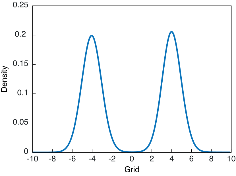
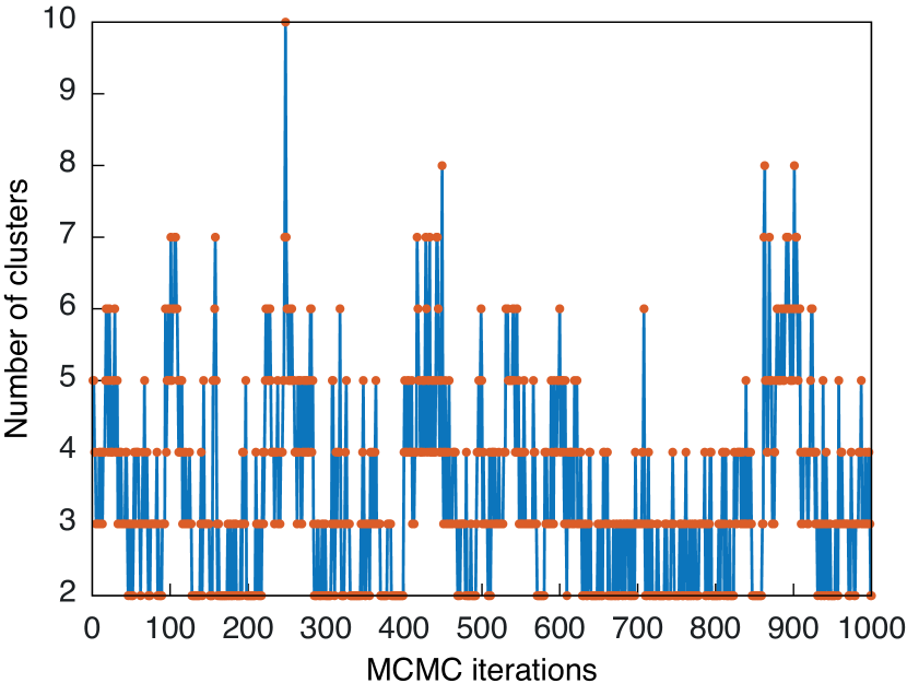
Figure 1: Plots from plot_mcmc executable: density estimate (left), histogram (center) and traceplot (right) of the number of clusters. The example refers to the DirichletMixing module described in Section 5.2.

5.2.2 An example through the Python interface

As mentioned before, we also provide (bayesmixpy), a Python interface that does not require users to use the terminal. To install the bayesmixpy package, navigate to the python sub-folder and execute in the terminal “python3 -m pip install -e .”. Once it is installed, the package provides the build_bayesmix() and run_mcmc() functions. The former installs the executable while the latter is used to run the MCMC chains. Below, we provide a hands-on example.

First, we build BayesMix:

⬇

from bayesmixpy import build_bayesmix, run_mcmc

build_bayesmix(nproc=4)

>>> …

>>> export the environment variable BAYESMIX_EXE=<BAYESMIX_PATH>/build/run_mcmc

Observe that the last output line specifies the location of the executable and asks users to export the environmental variable BAYESMIX_EXE. We can do it directly in Python as follows

⬇

import os

os.environ["BAYESMIX_EXE"] = "<BAYESMIX_PATH>/build/run_mcmc"

where <BAYESMIX_PATH>/build/run_mcmc is the path printed by build_bayesmix.

We are now ready to declare our model. We assume a DirichletMixing as mixing and a NNIGHierarchy as hierarchy. The following code snippet specifies that the “total mass” parameter of the Dirichlet process is fixed to $1.0$, the parameters of the Normal-Inverse-Gamma prior are fixed to $(\mu_{0},\lambda,a,b)=(0.0,0.1,2.0,2.0)$ and we will run Neal2Algorithm for 1,500 iterations, discarding the first 500 as burn-in.

⬇

dp_params = """

fixed_value {

totalmass: 1.0

}

"""

\parg0_params = """

fixed_values {

mean: 0.0

var_scaling: 0.1

shape: 2.0

scale: 2.0

}

"""

\paralgo_params = """

algo_id: "Neal2"

rng_seed: 20201124

iterations: 1500

burnin: 500

init_num_clusters: 3

"""

Finally, we run the MCMC algorithm on some simulated data, as simply as:

⬇

import numpy as np

\pardata = np.concatenate([np.random.normal(size=100) - 3,

np.random.normal(size=100) + 3])

dens_grid = np.linspace(-6, 6, 1000)

log_dens, numcluschain, cluschain, bestclus = run_mcmc(

"NNIG", "DP", data, go_params, dp_params, algo_params,

dens_grid=dens_grid, return_clusters=True, return_num_clusters=True,

return_best_clus=True)

which returns the log of the predictive density evaluated at dens_grid for each iteration of the MCMC sampling, the chain of the number of clusters, the chain of the cluster allocations, and the best clustering obtained by minimizing the posterior expectation of Binder’s loss function. We summarize the inference in a plot as follows:

⬇

import matplotlib.pyplot as plt

\parfig, axes = plt.subplots(nrows=1, ncols=3, figsize=(20, 5))

\paraxes[0].hist(data, alpha=0.2, density=True)

for c in np.unique(bestclus):

data_in_clus = data[bestclus == c]

axes[0].scatter(data_in_clus, np.zeros_like(data_in_clus) + 0.01,

label="Cluster {0}".format(int(c) + 1))

axes[0].plot(dens_grid, np.exp(np.mean(log_dens, axis=0)), color="red", lw=3)

axes[0].legend(fontsize=16, ncol=2, loc=1)

axes[0].set_ylim(0, 0.3)

\par\parx, y = np.unique(numcluschain, return_counts=True)

axes[1].bar(x, y / y.sum())

axes[1].set_xticks(x)

\paraxes[2].vlines(np.arange(len(numcluschain)), numcluschain-0.3, numcluschain+0.3)

plt.show()

The output of the above code is displayed in Figure 2.

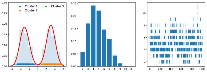
Figure 2: Output plot for the Python example: density estimate (left), histogram (center) and traceplot (right) of the number of clusters. The example refers to model (5) described in Section 5.2.

We also consider an example with bivariate datapoints, the faithful dataset, a well-known benchmark dataset for Bayesian density estimation and cluster detection. In this case, we assume that $f(\cdot\,|\,\tau)$ is the bivariate Gaussian density, with parameters $\tau=(\mu,\Psi=\Sigma^{-1})$ being the mean and precision matrix, respectively. A suitable prior for $\mu,\Psi$ is the Normal-Wishart distribution, i.e. $\mu\,|\,\Psi\sim\mathcal{N}_{2}(\mu_{0},(\lambda\Psi)^{-1})$, $\Psi\sim IW(\nu_{0},\Psi_{0})$, with $\E(\Psi)=\Psi_{0}/(\nu-2-1)$. To declare the model and run the MCMC algorithm, we can reuse most of the code of the univariate example, replacing the defintion of g0_params with:

⬇

g0_params = """

fixed_values {

mean {

size: 2

data: [3.484, 3.487]

}

var_scaling: 0.01

deg_free: 5

scale {

rows: 2

cols: 2

data: [1.0, 0.0, 0.0, 1.0]

rowmajor: false

}

}

"""

Posterior inference is summarized in Figure 3.

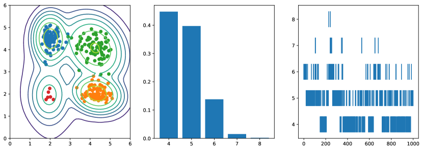
Figure 3: density estimate (left), histogram (center) and traceplot (right) of the number of clusters. The example refers to the faithful dataset in Section 5.2.

6 Performance benchmarking and comparisons

Here we compare the library BayesMix and the recently published BNPmix R package, which we have reviewed in Section 2, in terms of clustering quality and computational efficiency. All simulations were run on a Ubuntu 21.10 16 GB laptop machine. We consider three benchmark datasets for the comparison. The first two are the popular univariate galaxy and bivariate faithful datasets, both available in R. The third example is a simulated four-dimensional dataset, which we will refer to as highdim. It includes 10,000 points sampled from a Gaussian mixture with two equally weighted components, with mean $\mu_{4}=[2,2,2,2]$ and $-\mu_{4}$ respectively, and both covariance matrices equal to the identity matrix.

Since BNPmix focuses on Pitman-Yor processes and does not implement the Gamma prior for the total mass of the Dirichlet process, comparison is made using only Pitman-Yor mixtures with the same hyperparameter values for both libraries, including Pitman-Yor parameters and hierarchy hyperprior values. We test BayesMix using four different marginal algorithms – Neal2, Neal3, Neal8, and SplitMerge. The package BNPmix uses its own implementation of Neal2, which is referred to as mar, and the authors’ newly implemented importance conditional sampler, or ics for short. Each algorithm has been run for 5,000 iterations, with 1,000 iterations as burn-in period.

Autocorrelation plots for the number of clusters for all runs are displayed in Figure 4. BayesMix algorithms show better mixing properties of the MCMC chain, particularly in the bivariate galaxy case, where BNPmix struggles to reduce to zero the autocorrelation for large lags.

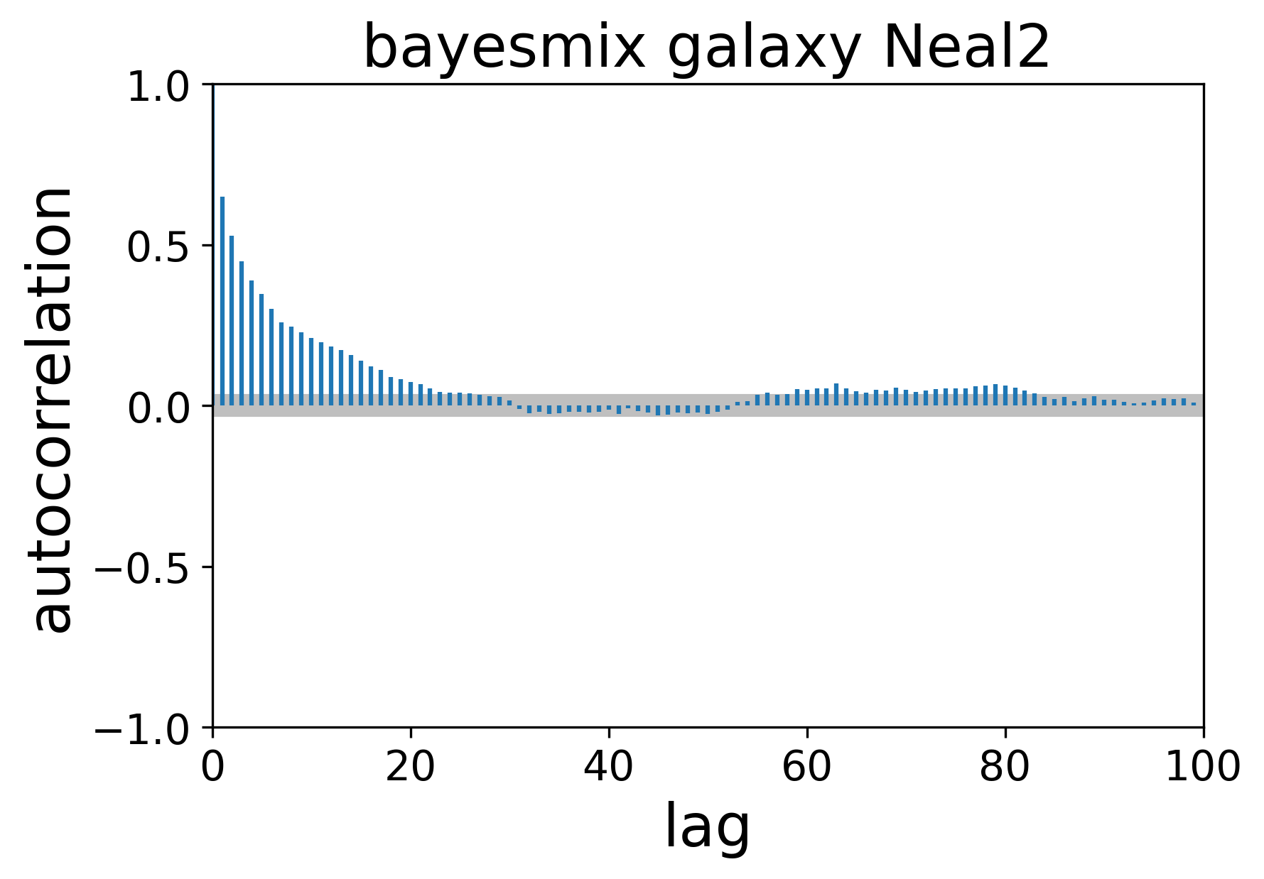
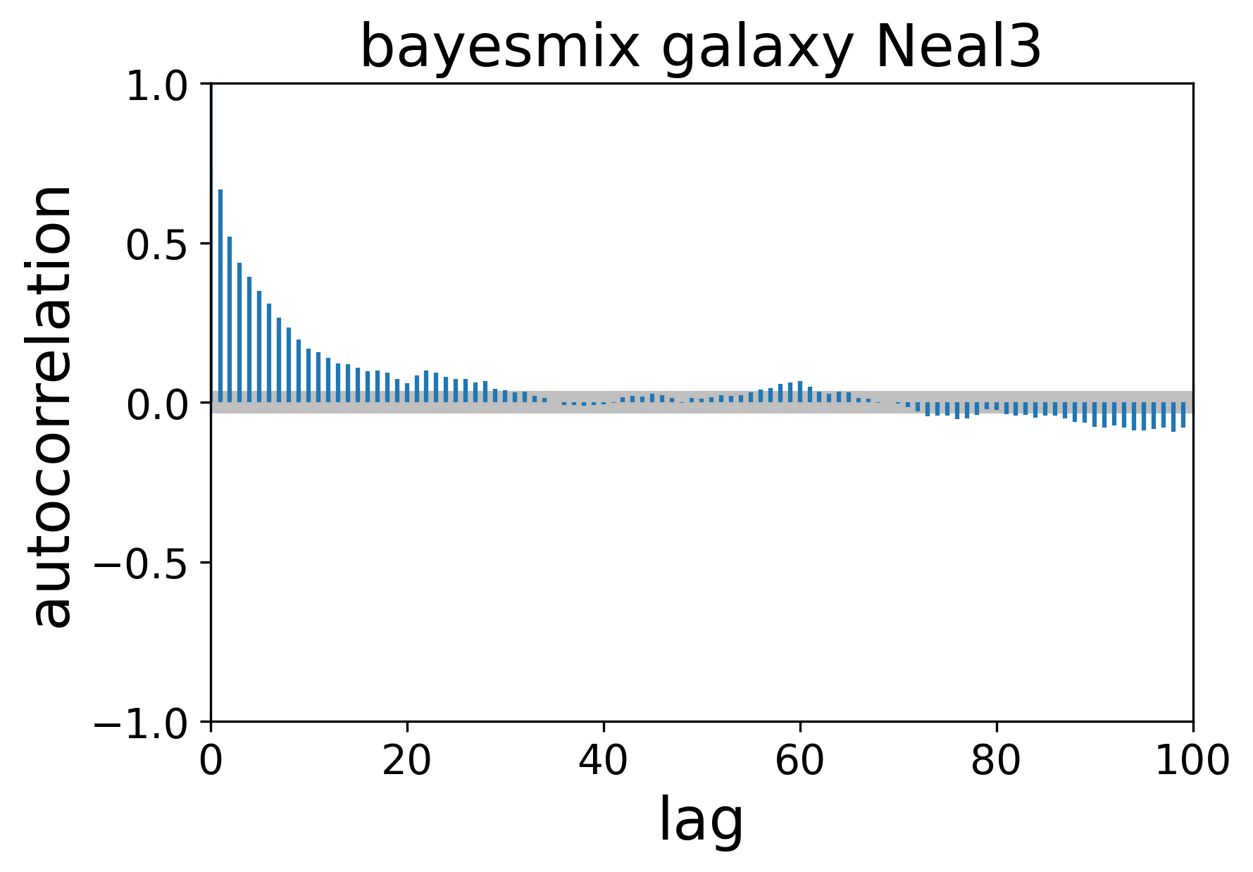
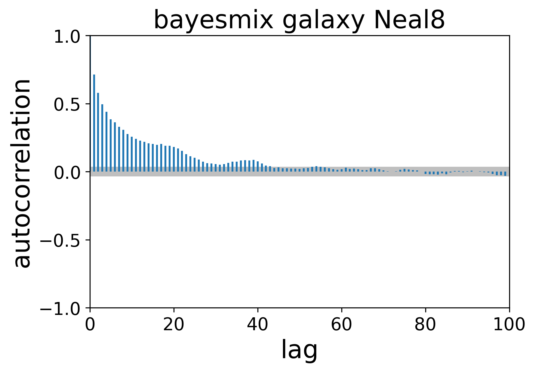
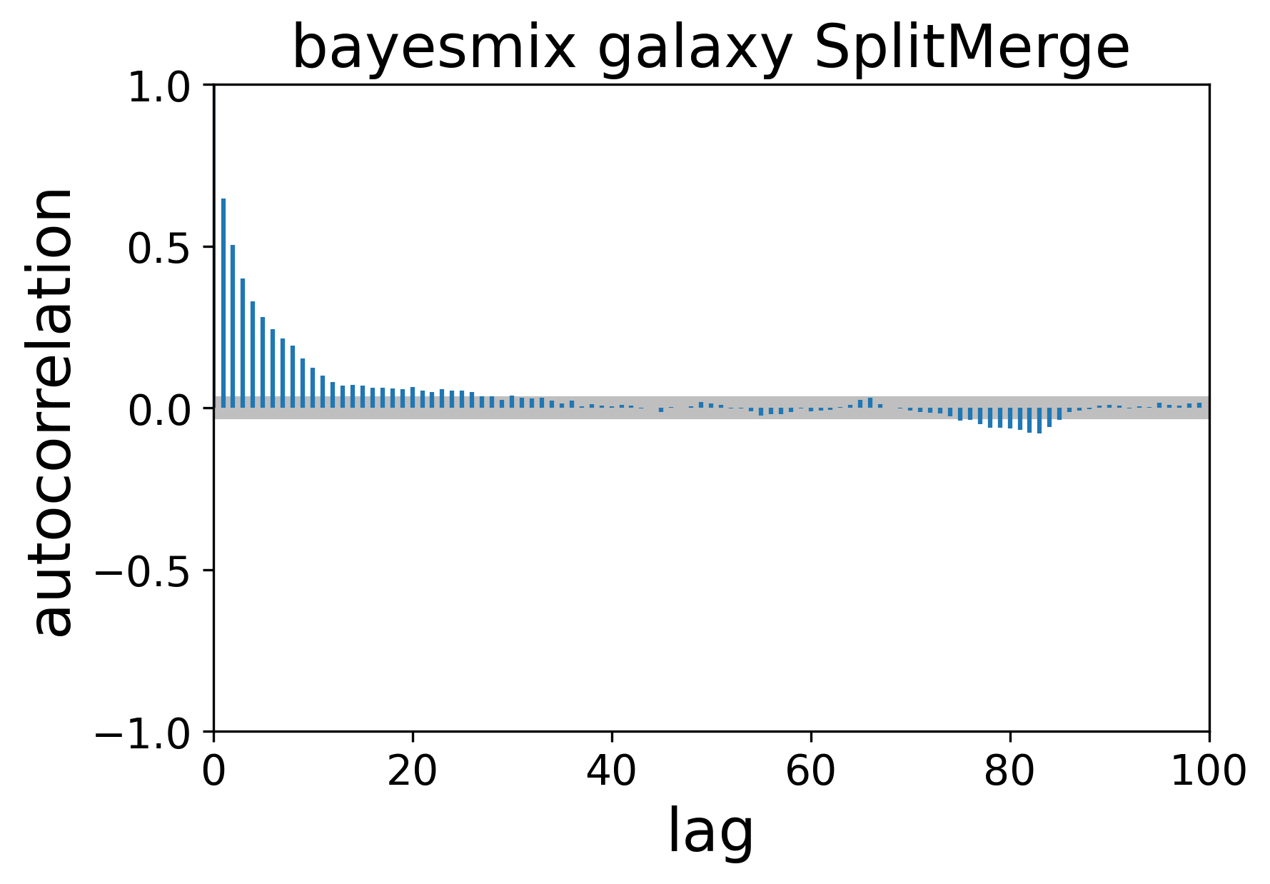
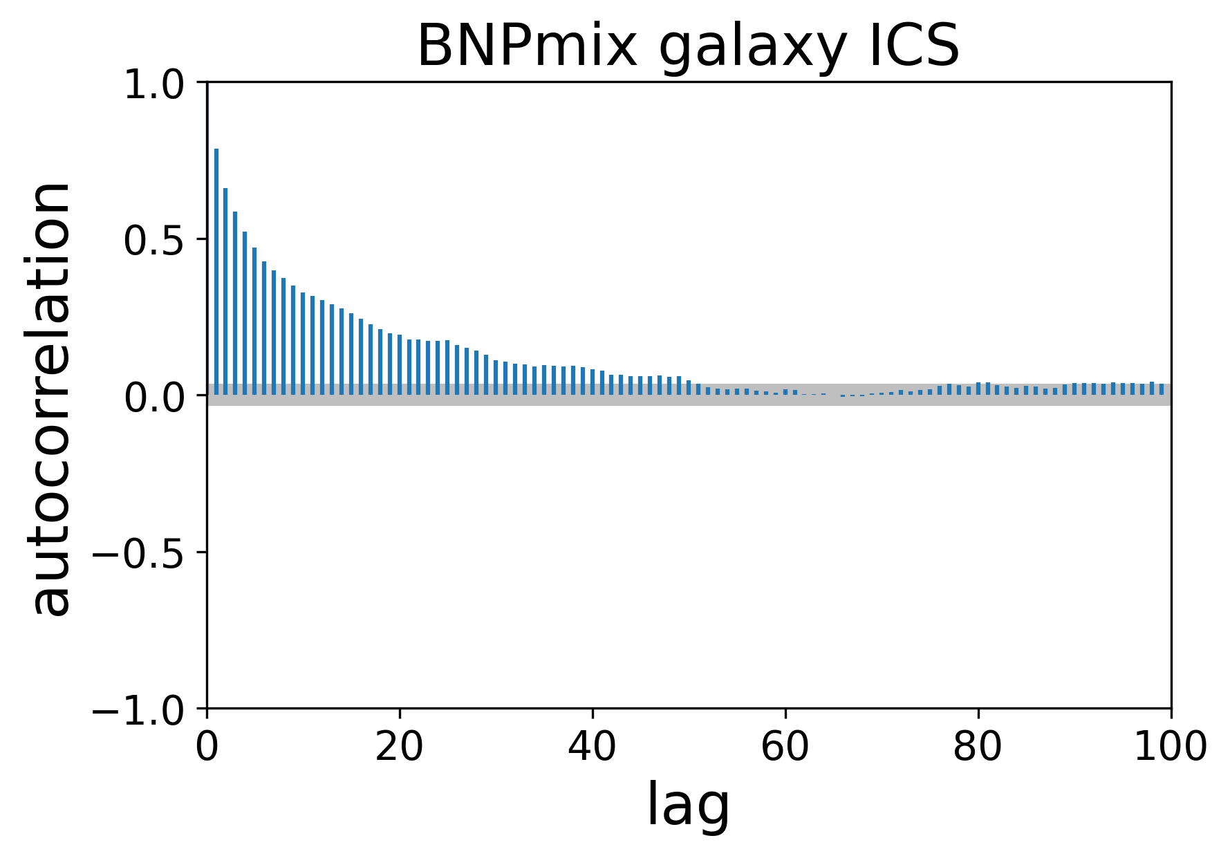
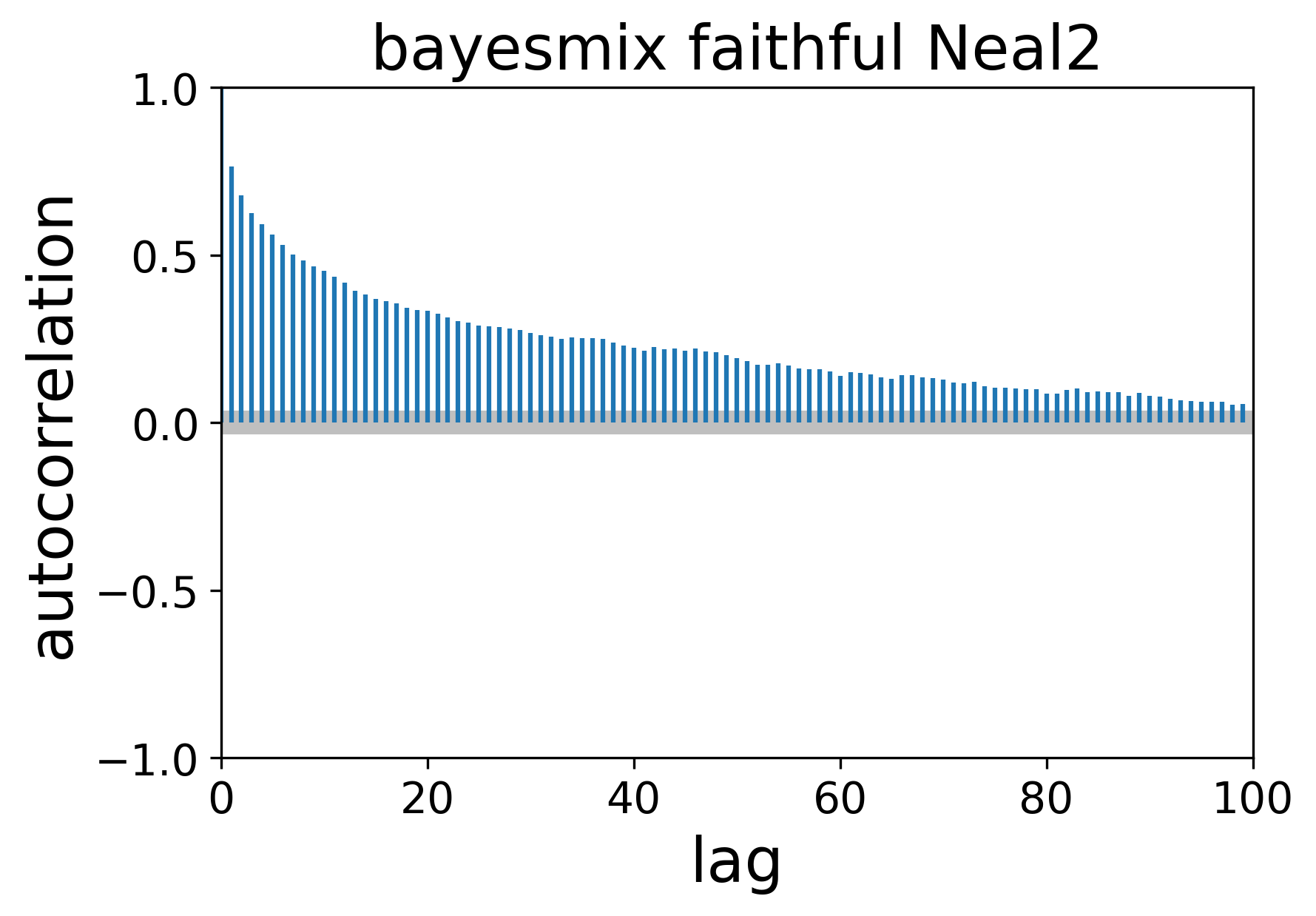
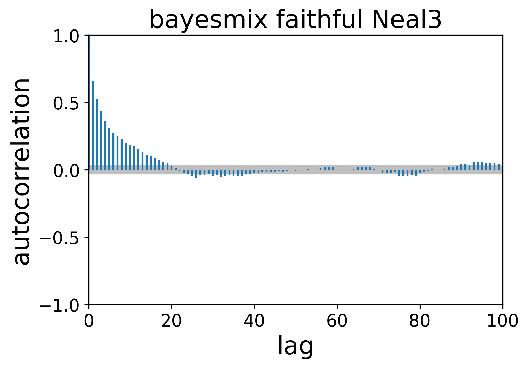
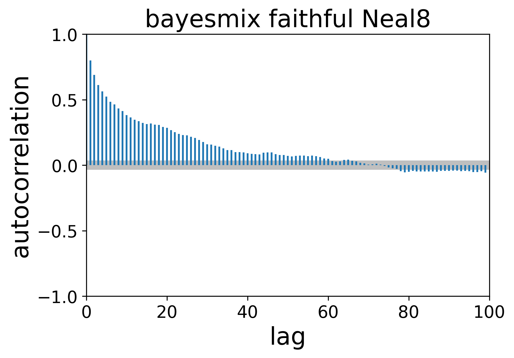
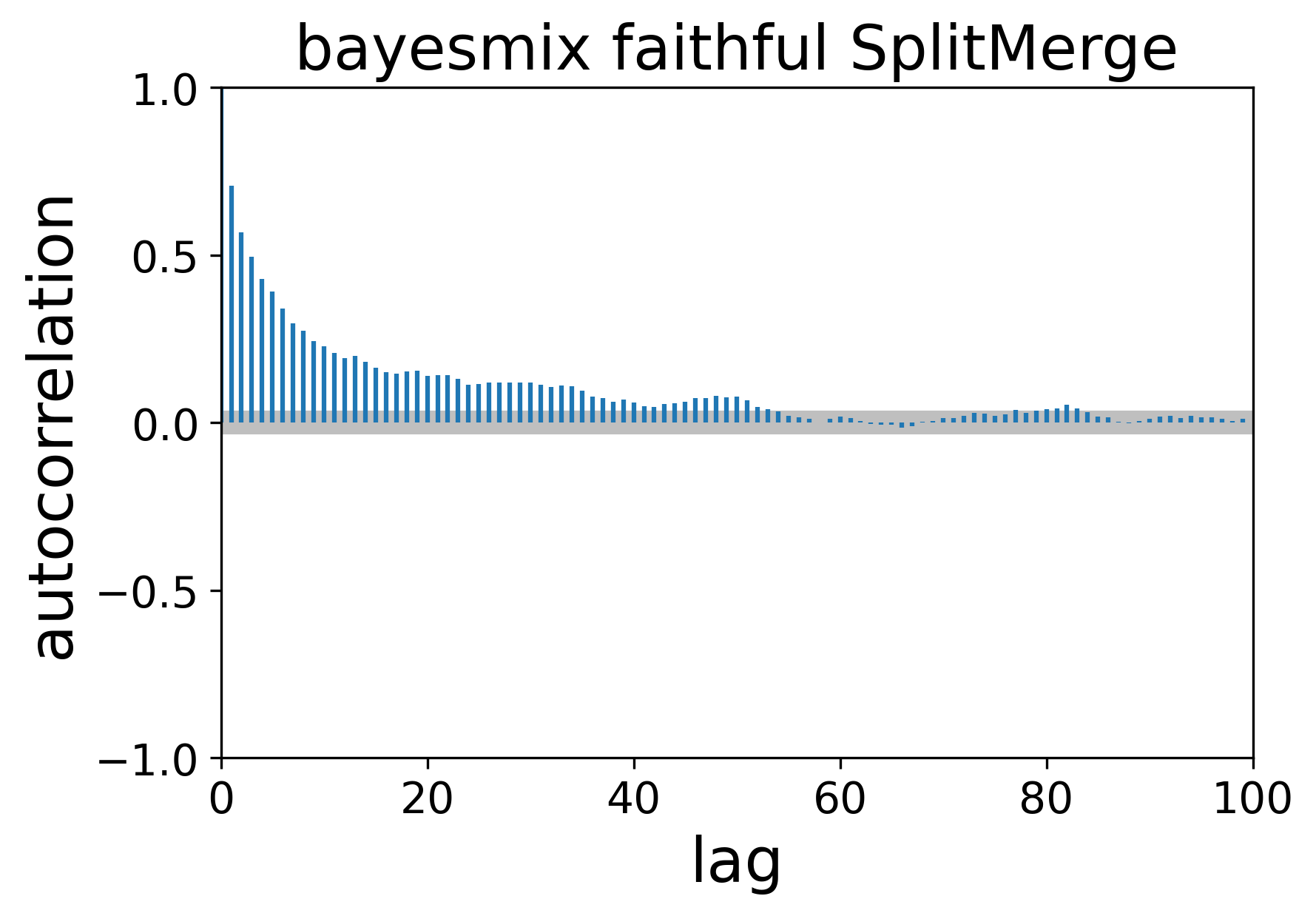
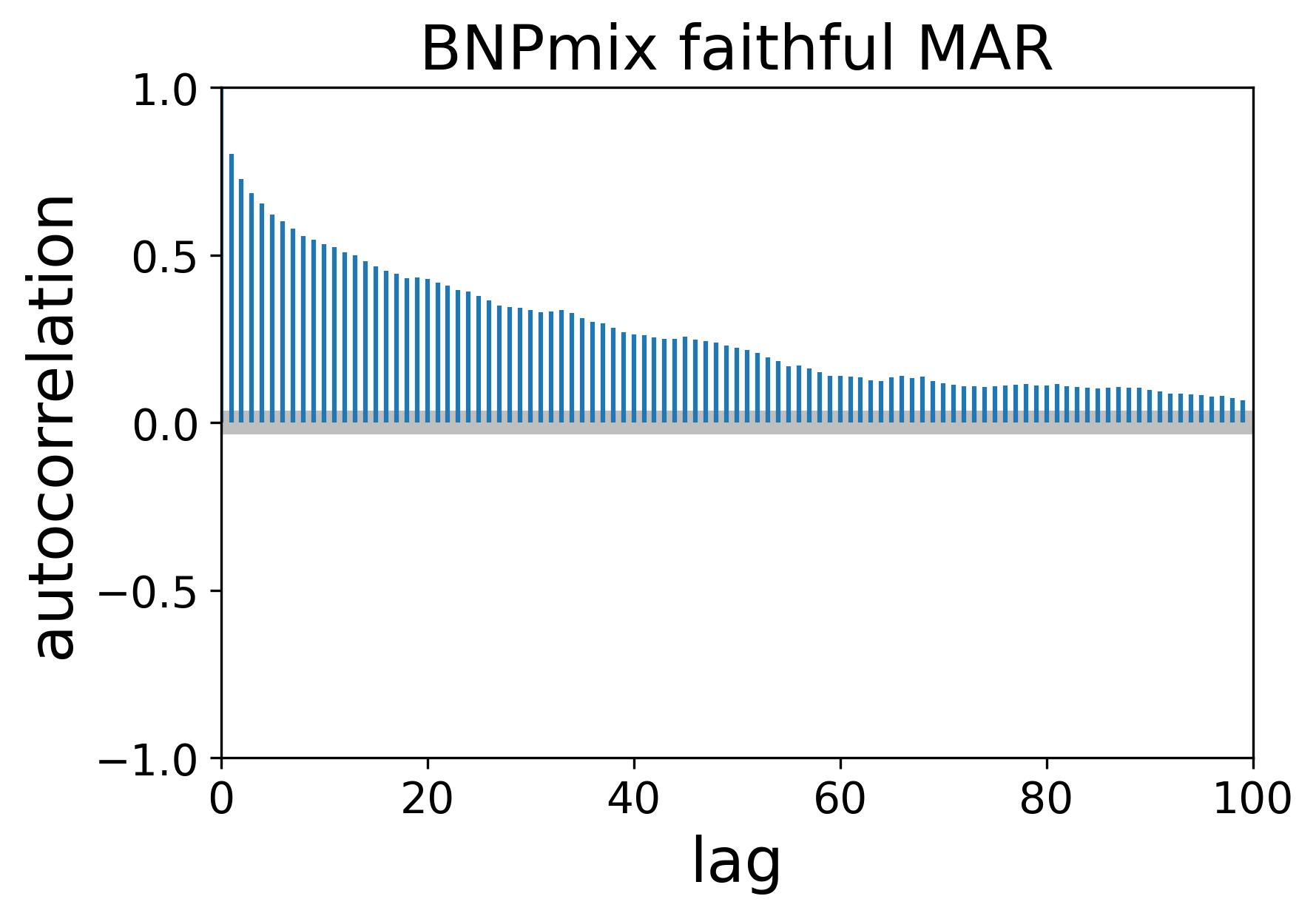
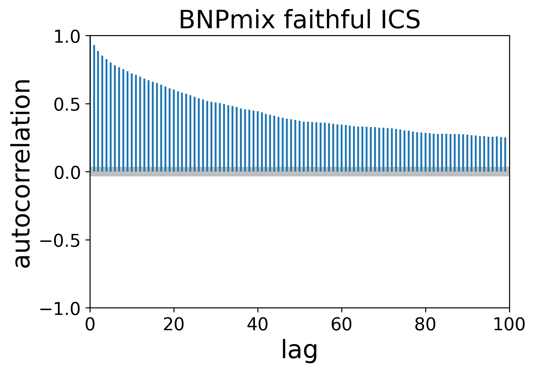
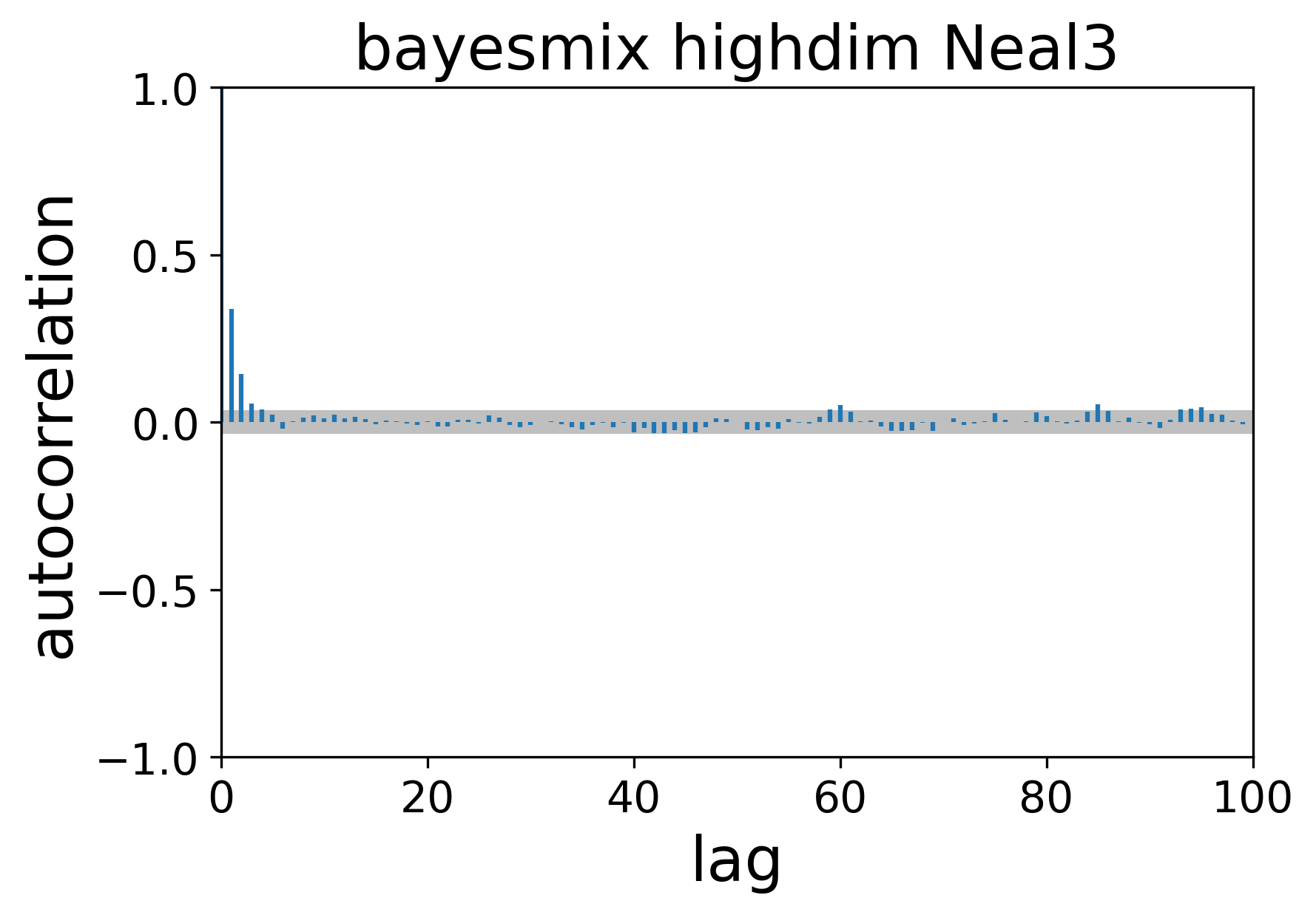
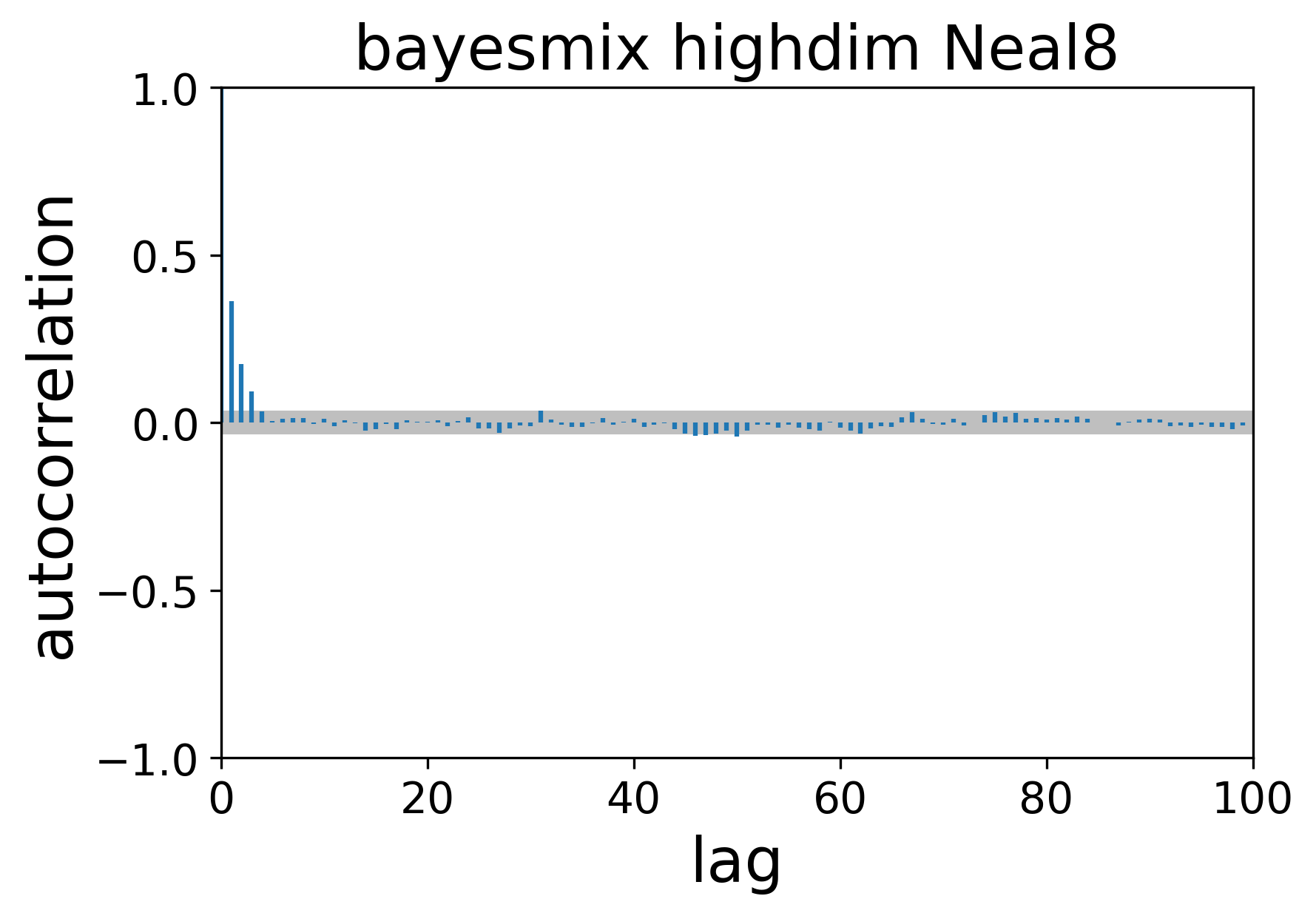
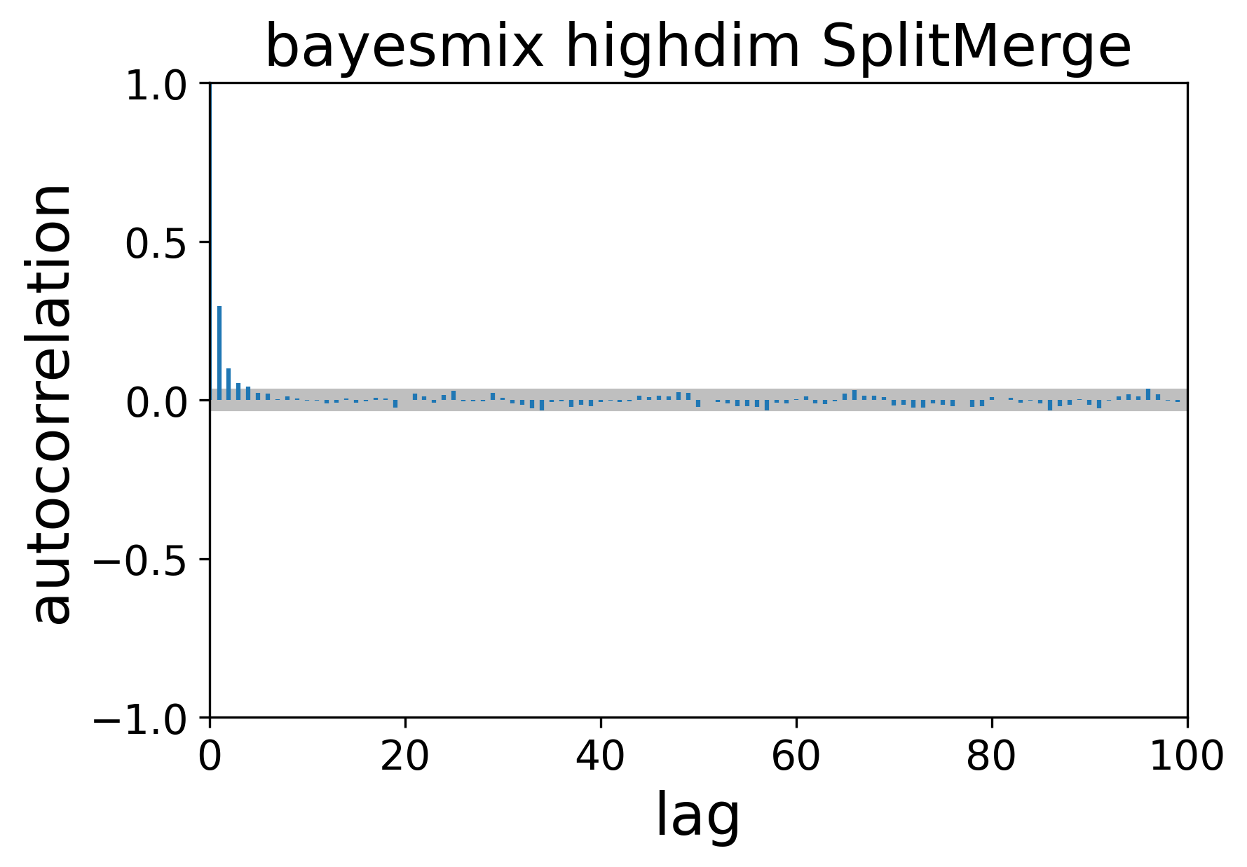
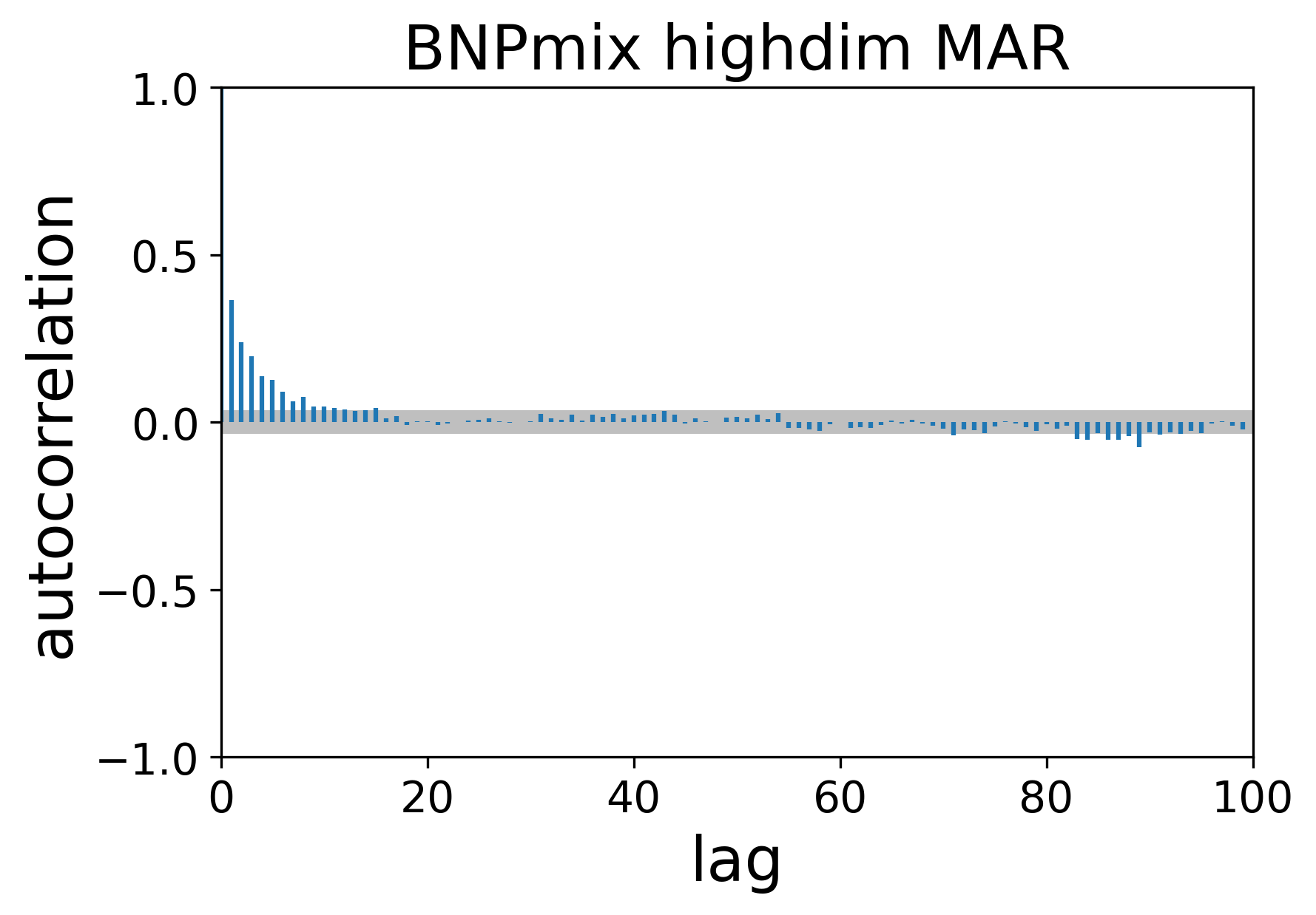
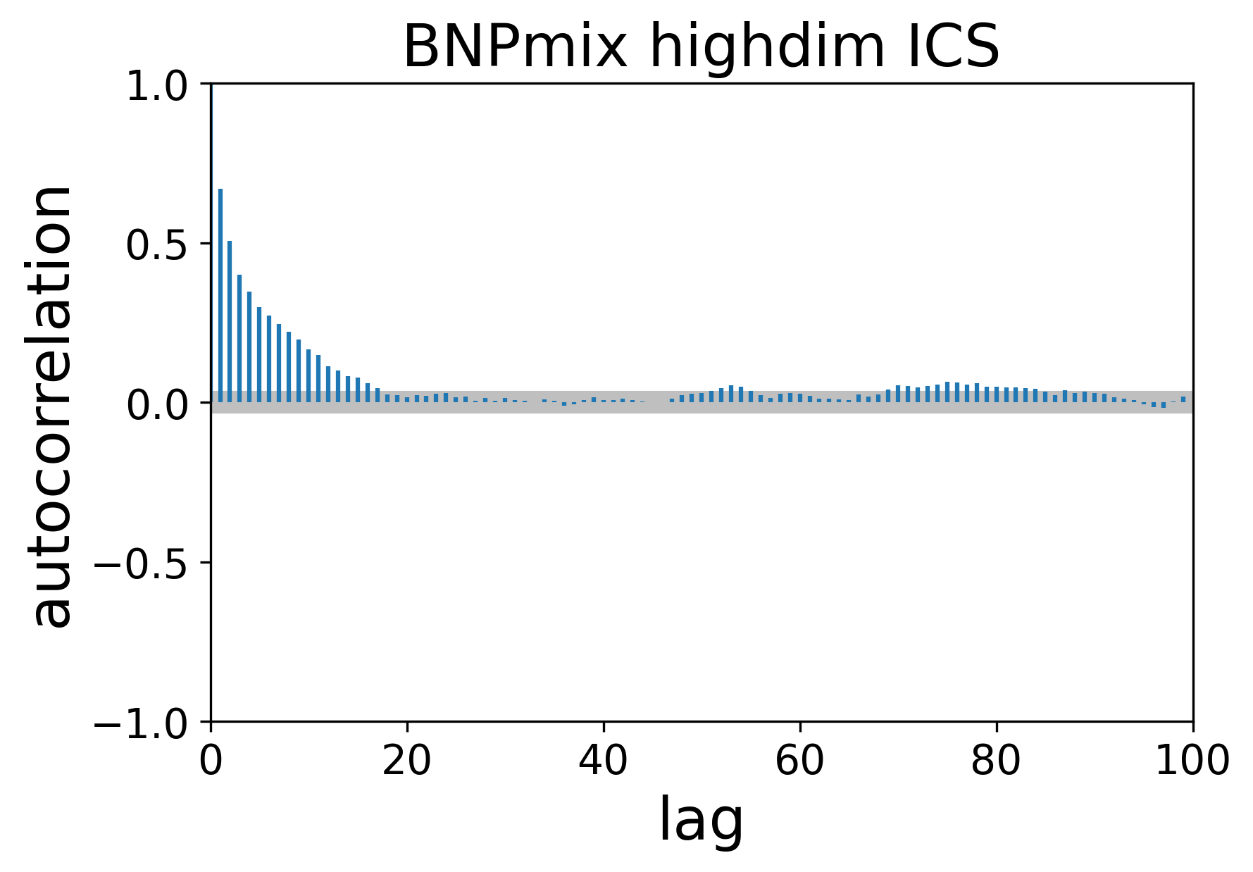
Figure 4: Comparison between autocorrelation plots on the number of clusters of the galaxy (top two rows), faithful (middle two rows), and highdim (bottom two rows) datasets

As far as computational efficiency is concerned, we report Effective Sample Size (ESS), running times, and ESS-over-time ratio of the MCMC simulations for the above tests in Tables 3, 4, and 5. ESS measures the quality of a chain in terms of equivalent, hypothetical sample size of independent observations. All BayesMix algorithms perform much better than BNPmix ones in terms of ESS while achieving comparable or lower running times. Neal2, i.e. the same algorithm as BNPmix’s mar, and Neal3 stand out as being particularly efficient as quantified by the three metrics, especially as the datapoint dimension grows larger (faithful and highdim).

	algorithm	ESS	time	ESS/time
BNPmix	mar	338.562	0.827	409.469
	ics	162.128	0.842	192.438
BayesMix	Neal2	337.467	0.370	912.073
	Neal3	340.332	0.611	557.009
	Neal8	191.580	0.589	325.263
	SplitMerge	400.551	1.218	328.860

Table 3: Comparison of metrics for the galaxy dataset

	algorithm	ESS	time	ESS/time
BNPmix	mar	36.288	3.733	9.721
	ics	15.499	1.949	7.954
BayesMix	Neal2	80.648	1.823	44.239
	Neal3	394.709	4.796	82.300
	Neal8	139.419	5.746	24.264
	SplitMerge	217.788	12.278	17.738

Table 4: Comparison of metrics for the faithful dataset

	algorithm	ESS	time	ESS/time
BNPmix	mar	978.471	1063.740	0.920
	ics	426.749	47.084	9.064
BayesMix	Neal2	1578.956	44.866	35.193
	Neal3	1861.819	166.151	11.206
	Neal8	1617.569	296.635	5.453
	SplitMerge	1865.773	870.494	2.143

Table 5: Comparison of metrics for the highdim dataset

As a final example for this comparison, we have simulated ten-dimensional datapoints from a Gaussian mixture with two well- separated components (with equal weights). As for highdim, the sample size is 10,000. All algorithms in BayesMix but Neal2 have been able to correctly distinguish the two clusters, whereas BNPmix failed to do so, identifying only one. The four- and ten-dimensional examples show that BayesMix has a scalable approach that works even with large, high-dimensional datasets.

7 Topics for expert users

The goal of this section is to give an example on how new users can extend the library by implementing a new Mixing or Hierarchy. To do so, the C++ code structure and the APIs of each base class must be explained in greater detail.

We give more details on the main building blocks in BayesMix. We follow an object-oriented approach and we adopt a combination of runtime and compile-time polymorphism based on inheritance and templates, using the so called curiously recurring template pattern (CRTP), as explained in Sections 7.1 and 7.2.

7.1 The Mixing module

As previously mentioned, a Mixing represents the prior distribution over the weights $\bm{w}$ and the associated EPPF. The AbstractMixing class defines the following API:

⬇

class AbstractMixing {

public:

virtual void initialize() = 0;

\parvirtual double get_mass_existing_cluster(

const unsigned int n, const bool log, const bool propto,

std::shared_ptr<AbstractHierarchy> hier,

const Eigen::RowVectorXd &covariate=Eigen::RowVectorXd(0));

\parvirtual double get_mass_new_cluster(

const unsigned int n, const bool log, const bool propto,

const unsigned int n_clust,

const Eigen::RowVectorXd &covariate=Eigen::RowVectorXd(0));

\parvirtual Eigen::VectorXd get_mixing_weights(

const bool log, const bool propto,

const Eigen::RowVectorXd &covariate = Eigen::RowVectorXd(0));

\parvirtual void update_state(

const std::vector<std::shared_ptr<AbstractHierarchy>> &unique_values,

const std::vector<unsigned int> &allocations) = 0;

};

In addition to these methods, AbstractMixing defines input-output functionalities discussed in Section 7.4.

The get_mass_existing_cluster() and get_mass_new_cluster() methods evaluate the EPPF $\Phi$. Specifically, get_mass_existing_cluster() evaluates $\Phi(n_{1},\ldots,n_{h}+1,\ldots,n_{k})=f_{1}(n_{h}+1,n,\theta)$ for a given $h$, while get_mass_new_cluster() evaluates $\Phi(n_{1},\ldots,n_{h},\ldots,n_{k}+1)=f_{2}(k,n,\theta)$ as defined in (4). Instead, get_mixing_weights() returns the vector of weights $\bm{w}$. Both methods used to evaluate the EPPF take as input the number n of observations in the model, as well as two boolean flags (propto, log) specifying if the result must be returned up to a proportionality constant and in log-scale. The get_mass_existing_cluster() method also receives a pointer to the Hierarchy the cluster represents. Note that the three methods take as input a vector of covariates, which is the empty vector by default and can be used to define dependent mixture models, for instance, by assuming the dependency logit stick breaking prior implemented in LogitSBMixing.

The update_state() method allows the child classes to assume hyperpriors on all the parameters. The update_state() method is used to sample parameters $\bm{w},m$ and additional hyperparameters from their full conditional.

Child classes do not inherit directly from AbstractMixing, but rather from a template class which in turn inherits from AbstractMixing, in the following way:

⬇

template <class Derived, typename State, typename Prior>

class BaseMixing : public AbstractMixing {

…

}

The BaseMixing class allows for more flexible code since it is templated over two objects representing the State and the Prior. For instance, in the case of a Pitman-Yor process, the state is defined as:

⬇

namespace PitYor {

struct State {

double strength, discount;

};

};

but more complex objects can be used as well. Moreover, BaseMixing implements several virtual methods from the AbstractMixing class, so that end users only need to focus on the code that is specific to a given model. For instance, a marginal mixing such as DirichletProcess only needs to implement the following methods:

⬇

void update_state(

const std::vector<std::shared_ptr<AbstractHierarchy>> &unique_values,

const std::vector<unsigned int> &allocations) override;

\pardouble mass_existing_cluster(

const unsigned int n, const bool log, const bool propto,

std::shared_ptr<AbstractHierarchy> hier) const override;

\pardouble mass_new_cluster(

const unsigned int n, const bool log, const bool propto,

const unsigned int n_clust) const override;

and some input-output functionalities. Instead, a conditional mixing such as TruncatedSBMixing implements the following functions:

⬇

void update_state(

const std::vector<std::shared_ptr<AbstractHierarchy>> &unique_values,

const std::vector<unsigned int> &allocations) override;

\parEigen::VectorXd get_weights(const bool log, const bool propto) const override;

7.2 The Hierarchy module

The Hierarchy module represents the Bayesian model

$$y_{j}\,|\,\tau \stackrel{{\scriptstyle\mbox{\scriptsize iid}}}{{\sim}}f(\cdot\,|\,\tau),\quad j=1,\ldots,l$$ (6)

$$\tau \sim G_{0}$$

Where $f(\cdot\,|\,\cdot)$ is the mixture component and $G_{0}$ the base measure. Given the model (6), we are interested in: ($i$) evaluating the (log) likelihood function $f(x\,|\,\tau)$ for a given $x$, ($ii$) sampling from the prior model $\tau\sim G_{0}$, and ($iii$) sampling from the full conditional of $\tau\,|\,y_{1},\ldots,y_{\ell}$. Each of these goals is delegated to a different class, namely the Likelihood, the PriorModel, and the Updater. Then a Hierarchy class is in charge of making Likelihood, PriorModel, and Updater communicate with each other and provides a common API for all possible models.

The choice of separating Likelihood, PriorModel, and Updater allows for great flexibility. In fact, we could have different Hierarchy classes that employ the same Likelihood but a different PriorModel. Moreover, different Updaters can be used. If the model is conjugate or semi-conjugate, a specific SemiConjugateUpdater is usually preferred. If this is not the case, we provide off-the-shelf RandomWalkUpdater and MALAUpdater that implement a random-walk Metropolis-Hastings move or a Metropolis-adjusted Langevin algorithm move, which can be used for any combination of Likelihood and PriorModel. As a consequence, users do not need to code an Updater if they want to implement a new model.

Throughout this section, we consider the illustrative example where $\tau=(\mu,\sigma^{2})$, $f(\cdot\,|\,\tau)=\mathcal{N}(\cdot\,|\,\mu,\sigma^{2})$ is the univariate Gaussian density and $G_{0}(\mu,\sigma^{2})=\mathcal{N}(\mu\,|\,\mu_{0},\sigma^{2}/\lambda)IG(\sigma^{2}\,|\,a,b)$ is the Normal-inverse-Gamma distribution.

The Hierarchy module and all its sub-modules (Likelihood, PriorModel, State and Updater) achieve runtime polymorphism through an abstract interface (which establishes which operations can be performed by the end user) and employing the Curiously Recurring Template Pattern (CRTP Coplien, 1995).

Let us explain the structure in more detail, starting with the Hierarchy module. First, an AbstractHierarchy defines the following API:

⬇

class AbstractHierarchy {

public:

double get_like_lpdf(

const Eigen::RowVectorXd &datum,

const Eigen::RowVectorXd &covariate) const;

\parvirtual void sample_prior() = 0;

\parvirtual void sample_full_cond(bool update_params) = 0;

\parvirtual void add_datum(

const int id, const Eigen::VectorXd &datum,

const bool update_params, const Eigen::VectorXd &covariate) = 0;

\parvirtual void remove_datum(

const int id, const Eigen::VectorXd &datum,

const bool update_params, const Eigen::VectorXd &covariate)) = 0;

};

In the code above, get_like_lpdf() evaluates the likelihood function $f(y\,|\,\tau)$ for a given datapoint, sample_prior() samples from $G_{0}$, and add_datum() (remove_datum()) are called when allocating (removing) a datum from the current cluster.

As in the case of Mixings, child classes inherit from a template class with respect to the Likelihood and the PriorModel from the BaseHierarchy class. Most of the methods in the API are implemented in this class. Thus, coding a new hierarchy is extremely simple within this framework, since only very few methods need to be implemented from scratch. All the hierarchies available so far inherit from this class and are reported in Table 1.

7.2.1 The Likelihood sub-module

The Likelihood sub-module represents the likelihood we have assumed for the data in a given cluster. Each Likelihood class represents the sampling model

$$y_{1},\ldots,y_{k}\,|\,\bm{\tau}\stackrel{{\scriptstyle\mbox{\scriptsize iid}}}{{\sim}}f(\cdot\,|\,\bm{\tau})$$

for a specific choice of the probability density function $f$.

In principle, the Likelihood classes are responsible only of evaluating the log-likelihood function given a specific choice of parameters $\bm{\tau}$. Therefore, a simple inheritance structure would seem appropriate. However, the nature of the parameters $\bm{\tau}$ can be very different across different models (think for instance of the difference between the univariate normal and the multivariate normal paramters). As such, we again employ CRTP to manage the polymorphic nature of Likelihood classes.

The AbstractLikelihood class provides the following common API:

⬇

class AbstractLikelihood {

public:

double lpdf(

const Eigen::RowVectorXd &datum,

const Eigen::RowVectorXd &covariate = Eigen::RowVectorXd(0)) const;

\parvirtual Eigen::VectorXd lpdf_grid(

const Eigen::MatrixXd &data,

const Eigen::MatrixXd &covariates = Eigen::MatrixXd(0, 0)) const = 0;

\parvirtual double cluster_lpdf_from_unconstrained(

Eigen::VectorXd unconstrained_params) const;

\parvirtual stan::math::var cluster_lpdf_from_unconstrained(

Eigen::Matrix<stan::math::var, Eigen::Dynamic, 1> unconstrained_params)

const;

\parvirtual bool is_multivariate() const = 0;

\parvirtual bool is_dependent() const = 0;

\parvirtual void add_datum(

const int id, const Eigen::RowVectorXd &datum,

const Eigen::RowVectorXd &covariate = Eigen::RowVectorXd(0)) = 0;

\parvirtual void remove_datum(

const int id, const Eigen::RowVectorXd &datum,

const Eigen::RowVectorXd &covariate = Eigen::RowVectorXd(0)) = 0;

\par\parvoid update_summary_statistics(const Eigen::RowVectorXd &datum,

const Eigen::RowVectorXd &covariate,

bool add);

\parvirtual void clear_summary_statistics() = 0;

};

First of all, we require the implementation of the lpdf() and lpdf_grid() methods, which simply evaluate the loglikelihood in a given point or in a grid of points (also in case of a dependent likelihood, i.e., in which covariates are associated to each observation). The cluster_lpdf_from_unconstrained() method allows the evaluation of the likelihood of the whole cluster starting from the vector of unconstrained parameters. This is a key method which is only needed if a Metropolis-like updater is used. Observe that the AbstractLikelihood class provides two such methods, one returning a double and one returning a stan::math::var. The latter is used to automatically compute the gradient of the likelihood via Stan’s automatic differentiation, if needed. In practice, users do not need to implement both methods separately, and can implement only one templated method; see the UniNormLikelihood example below. The add_datum() and remove_datum() methods manage the insertion and deletion of a data point in the given cluster, and update the summary statistics associated with the likelihood using the update_summary_statistics() method. Summary statistics (when available) are used to evaluate the likelihood function on the whole cluster, as well as to perform the posterior updates of $\bm{\tau}$. This usually gives a substantial speed-up.

Given this API, we define the BaseLikelihood class, which is a template class with respect to itself (thus enabling CRTP) and a State. The latter is a class which stores the parameters $\bm{\tau}$ and eventually manages the transformation in its unconstrained form (for Metropolis updaters), if any. The BaseLikelihood class is declared as follows:

⬇

template <class Derived, typename State>

class BaseLikelihood : public AbstractLikelihood

This class implements methods that are common to all the likelihoods, in order to minimize the code that end users need to implement. Note that every concrete implementation of a likelihood model inherits from such a class. The following likelihoods are currently implemented in BayesMix:

1. UniNormLikelihood, that is $y\,|\,\mu,\sigma^{2}\sim\mathcal{N}(\mu,\sigma^{2})$, $\mu\in\mathbb{R}$, $\sigma^{2}>0$.

2. MultiNormLikelihood, that is $y\,|\,\mu,\Sigma\sim\mathcal{N}_{d}(\mu,\Sigma)$, $\mu\in\mathbb{R}^{d}$, $\Sigma$ a symmetric and positive definite covariance matrix.

3. FALikelihood, that is $y\,|\,\mu,\Sigma\sim\mathcal{N}_{d}(\mu,\Sigma+\Lambda\Lambda^{\top})$, $\mu\in\mathbb{R}^{d}$, $\Sigma=\text{diag}(\sigma^{2}_{1},\ldots,\sigma^{2}_{d})$, $\sigma^{2}_{j}>0$, $\Lambda$ a $d\times p$ matrix (usually $p\ll d$, hence the name factor-analyzer likelihood).

4. LinRegUniLikelihood, that is $y\,|\,\beta,\sigma^{2}\sim\mathcal{N}(x^{\top}\beta,\sigma^{2})$, $\beta\in\mathbb{R}^{d}$, $\sigma>0$. Here $x$ is a vector of covariates, meaning that this hierarchy is dependent.

5. UniLapLikelihood, that is $y\,|\,\mu,\lambda\sim\mathrm{Laplace}(\mu,\lambda)$, $\mu\in\mathbb{R}$, $\lambda>0$.

We report the code for UniNormLikelihood as an illustrative example:

⬇

class UniNormLikelihood

: public BaseLikelihood<UniNormLikelihood, State::UniLS> {

public:

UniNormLikelihood() = default;

\par~UniNormLikelihood() = default;

\parbool is_multivariate() const override { return false; };

\parbool is_dependent() const override { return false; };

\parvoid clear_summary_statistics() override;

\partemplate <typename T>

T cluster_lpdf_from_unconstrained(

const Eigen::Matrix<T, Eigen::Dynamic, 1> &unconstrained_params) const;

\parprotected:

double compute_lpdf(const Eigen::RowVectorXd &datum) const override;

\parvoid update_sum_stats(const Eigen::RowVectorXd &datum, bool add) override;

\pardouble data_sum = 0;

\pardouble data_sum_squares = 0;

};

7.2.2 The PriorModel sub-module

This sub-module represents the prior for the parameters in the likelihood, i.e.

$$\bm{\tau}\sim G_{0}$$

with $G_{0}$ being a suitable prior on the parameters space. We also allow for more flexible priors adding further level of randomness (i.e. the hyperprior) on the parameter characterizing $G_{0}$. Similarly to the case of Likelihood sub-module, we need to rely on a design pattern that can manage a wide variety of specifications. We rely once more on the CRTP approach, thus defining an API via a pure virtual class: AbstractPriorModel, which collects the methods each class should implement. This class is defined as follows:

⬇

class AbstractPriorModel {

public:

\parvirtual double lpdf(const google::protobuf::Message &state_) = 0;

\parvirtual double lpdf_from_unconstrained(

Eigen::VectorXd unconstrained_params) const;

\parvirtual stan::math::var lpdf_from_unconstrained(

Eigen::Matrix<stan::math::var,Eigen::Dynamic,1> unconstrained_params) const;

\parvirtual std::shared_ptr<google::protobuf::Message> sample(

ProtoHypersPtr hier_hypers = nullptr) = 0;

\parvirtual void update_hypers(

const std::vector<bayesmix::AlgorithmState::ClusterState> &states) = 0;

};

The lpdf() and lpdf_from_unconstrained() methods evaluate the log-prior density function at the current state $\bm{\tau}$ or its unconstrained representation. In particular, lpdf_from_unconstrained() is needed by Metropolis-like updaters; see below for further details. The sample() method generates a draw from the prior distribution. If hier_hypers is nullptr, the prior hyperparameter values are used. To allow sampling from the full conditional distribution in case of semi-congugate hierarchies, we introduce the hier_hypers parameter, which is a pointer to a Protobuf message storing the hierarchy hyperaprameters to use for the sampling. The update_hypers() method updates the prior hyperparameters, given the vector of all cluster states.

Given the API, we define the BasePriorModel class, which is declared as:

⬇

template <class Derived, class State, typename HyperParams, typename Prior>

class BasePriorModel : public AbstractPriorModel

Such a class is derived from AbstractPriorModel. It is a template class with respect to itself (for CRTP), a State class (which represents the parameters over which the prior is assumed) an HyperParams type (which is a simple struct that codes the parameters characterizing $G_{0}$) and a Prior (which codes hierarchical priors for the $G_{0}$ parameters for more flexible and robust prior models). Like in previous sub-modules, this class manages code exceptions and implements general methods. Every concrete implementation of a prior model must be defined as an inherited class of BasePriorModel. The library currently supports the following priors:

1. NIGPriorModel $\mu\,|\,\sigma^{2}\sim\mathcal{N}(\mu_{0},\sigma^{2}/\lambda)$, $\sigma^{2}\sim IG(a,b)$.

2. NxIGPriorModel $\mu\sim\mathcal{N}(\mu_{0},\sigma_{0}^{2})$, $\sigma^{2}\sim IG(a,b)$.

3. NWPriorModel $\mu\,|\,\Sigma\sim\mathcal{N}(\mu_{0},\Sigma/\lambda)$, $\Sigma\sim IW(\nu_{0},\Psi_{0})$.

4. MNIGPriorModel $\beta\,|\,\sigma^{2}\sim N_{p}(\mu,\sigma^{2}\Lambda^{-1})$, $\sigma^{2}\sim IG(a,b)$

5. FAPriorModel $\mu\sim\mathcal{N}_{p}(\widetilde{\mu},\psi I)$, $\Lambda\sim\mbox{DL}(\alpha)$, $\Sigma=\mbox{diag}(\sigma_{1},\ldots,\sigma_{p})$, $\sigma_{j}\stackrel{{\scriptstyle\mbox{\scriptsize iid}}}{{\sim}}IG(a,b)$, $j=1,\ldots,p$, where DL is the Dirichlet-Laplace distribution in Bhattacharya et al. (2015).

As an example, we report the implementation of the NIGPriorModel here below:

⬇

class NIGPriorModel : public BasePriorModel<

NIGPriorModel, State::UniLS, Hyperparams::NIG, bayesmix::NNIGPrior> {

public:

using AbstractPriorModel::ProtoHypers;

\parusing AbstractPriorModel::ProtoHypersPtr;

\parNIGPriorModel() = default;

\par~NIGPriorModel() = default;

\pardouble lpdf(const google::protobuf::Message &state_) override;

\partemplate <typename T>

T lpdf_from_unconstrained(

const Eigen::Matrix<T, Eigen::Dynamic, 1> &unconstrained_params) const {

Eigen::Matrix<T, Eigen::Dynamic, 1> constrained_params =

State::uni_ls_to_constrained(unconstrained_params);

T log_det_jac = State::uni_ls_log_det_jac(constrained_params);

T mean = constrained_params(0);

T var = constrained_params(1);

T lpdf = stan::math::normal_lpdf(mean, hypers->mean,

sqrt(var / hypers->var_scaling)) +

stan::math::inv_gamma_lpdf(var, hypers->shape, hypers->scale);

\parreturn lpdf + log_det_jac;

};

\parState::UniLS sample(ProtoHypersPtr hier_hypers = nullptr) override;

\parvoid update_hypers(const std::vector<bayesmix::AlgorithmState::ClusterState>

&states) override;

\parvoid set_hypers_from_proto(

const google::protobuf::Message &hypers_) override;

\parstd::shared_ptr<bayesmix::AlgorithmState::HierarchyHypers> get_hypers_proto()

const override;

\parprotected:

void initialize_hypers() override;

};

7.2.3 The Updater sub-module

The Updater module implements the machinery to provide a sampling from the full conditional distribution of a given hierarchy. Again, we rely on CRTP and define the API in the AbstractUpdater class as follows:

⬇

class AbstractUpdater {

public:

virtual bool is_conjugate() const;

\parvirtual void draw(AbstractLikelihood &like, AbstractPriorModel &prior,

bool update_params) = 0;s

};

Here is_conjugate() declares whether the updater is meant to be used for a semi-conjugate hierarchy. The draw method is the key method of every updater: it receives like and prior as input, and updates the State (which is stored inside the Likelihood) by sampling it from conditional distribution $\bm{\tau}\,|\,y_{1},\ldots,y_{h}$, where the $y_{j}$’s are the data associated to one specific cluster. As already mentioned, when (6) is semi-conjugate, problem-specific updaters can be easily implemented by inheriting from the SemiConjugateUpdater; see, for instance, the code below.

⬇

class NNIGUpdater: public SemiConjugateUpdater<UniNormLikelihood, NIGPriorModel> {

public:

NNIGUpdater() = default;

~NNIGUpdater() = default;

\parbool is_conjugate() const override { return true; };

\parProtoHypers compute_posterior_hypers(AbstractLikelihood &like,

AbstractPriorModel &prior) override;

};

In particular, note that this class does not implement any draw() method. In fact, since the model is semi-conjugate, we exploit the PriorModel draw function but using updated parameters, which are computed by the compute_posterior_hypers() method.

If the model is not semi-conjugate, we suggest using RandomWalkUpdater or MALAUpdater, which sample from the full conditional distribution of $\bm{\tau}$ using a Metropolis-Hastings move. In this case, the following methods must be implemented in the Likelihood class:

⬇

template <typename T>

T cluster_lpdf_from_unconstrained(

const Eigen::Matrix<T, Eigen::Dynamic, 1> &unconstrained_params) const;

while the prior should implement the following:

⬇

template <typename T>

T lpdf_from_unconstrained(

const Eigen::Matrix<T, Eigen::Dynamic, 1> &unconstrained_params) const;

For instance, when $f$ is the univariate Gaussian density, the unconstrained parameters are $(\mu,\log(\sigma^{2}))$. To evaluate the likelihood, it is sufficient to transform $\log(\sigma^{2})$ using the exponential function. Instead, to evaluate the prior, one should take care of the correction in the density function due to the change of variables.

7.2.4 The State sub-module

States are classes used to store parameters $\tau_{h}$’s of every mixture component. Their main purpose is to handle serialization and de-serialization of the state; see also Section 7.4. Moreover, they allow to go from the constrained to the unconstrained representation of the parameters (and viceversa) and compute the associated determinant of the Jacobian appearing in the change of density formula. All states inherit from a BaseState:

⬇

class BaseState {

public:

int card;

using ProtoState = bayesmix::AlgorithmState::ClusterState;

\parvirtual Eigen::VectorXd get_unconstrained() { throw std::runtime_error("…"); }

virtual void set_from_unconstrained(const Eigen::VectorXd &in) {

throw std::runtime_error("…"); }

virtual double log_det_jac() { throw std::runtime_error("…"); }

\parvirtual void set_from_proto(const ProtoState &state_, bool update_card) = 0;

virtual ProtoState get_as_proto() const = 0;

std::shared_ptr<ProtoState> to_proto() const {

return std::make_shared<ProtoState>(get_as_proto());

}

};

Depending on the chosen Updater, the methods get_unconstrained(), set_from_unconstrained() and log_det_jac() might never be called. Therefore, we do not force users to implement them. Instead, the set_from_proto() and get_as_proto() are fundamental as they allow the interaction with Google’s Protocol Buffers library; see Section 7.4 for more detail.

7.3 The Algorithm module

Mixing and Hierarchy classes are combined together by an Algorithm. Algorithms are direct implementation of MCMC samplers, such as Neal’s Algorithm 2/3/8 and the blocked Gibbs sampler from Ishwaran and James (2001). All algorithms must inherit from the BaseAlgorithm class:

⬇

class BaseAlgorithm {

protected:

Eigen::MatrixXd data;

Eigen::MatrixXd hier_covariates;

Eigen::MatrixXd mix_covariates;

\parstd::vector<unsigned int> allocations;

std::vector<std::shared_ptr<AbstractHierarchy>> unique_values;

std::shared_ptr<BaseMixing> mixing;

\parvirtual void sample_allocations() = 0;

virtual void sample_unique_values() = 0;

\parvirtual void step() {}

\parpublic:

void run(BaseCollector *collector);

virtual Eigen::MatrixXd eval_lpdf(

BaseCollector *const collector, const Eigen::MatrixXd &grid,

const Eigen::MatrixXd &hier_covariates = Eigen::MatrixXd(0, 0),

const Eigen::MatrixXd &mix_covariates = Eigen::MatrixXd(0, 0)) = 0;

};

The Algorithm class saves the data and (optionally) two set of covariates: hier_covariates and mix_covariates. Therefore, it is trivial to extend the code to more general models to accommodate for covariate-dependent likelihoods and/or mixings. Moreover, the Algorithm also stores the cluster allocation variables (allocations), the hierachies representing the mixture components (unique_values) and the mixing (mixing). The last two objects are stored through pointers to the corresponding base class, to achieve runtime polymorphism.

The basic method from Algorithm is step() which performs a Gibbs sampling step calling the appropriate update methods for all the blocks of the model. A run() method is used to run the MCMC chain, i.e. run() calls step() for a user-specified number of iterations, possibly discarding an initial burn-in phase. The goal of MCMC simulations is to collect samples from the posterior distribution, which must be stored for later use. Hence, the run() receives as input an instance of BaseCollector which is indeed in charge of storing the visited states either in memory (RAM) or by saving in a file; see Section 7.4 for further details.

Since one of the main goals of mixture analysis is density estimation, an Algorithm must be also able to evaluate the mixture density on a fixed grid, given the visited samples. This is achieved by the eval_lpdf() method.

All the algorithms implemented in BayesMix are listed in Table 2.

7.4 I/O and cross-language functionalities

There is a final building block of BayesMix, that is the management of input / output (I/O). Most of C++ based packages for Bayesian inference, such as Stan (Stan Development Team, 2019) and JAGS (Plummer, 2017), rely on tabular formats to save the chains. Specifically, the output of an MCMC algorithm is collected in an array where each parameter is saved in a different column and the resulting object is then serialized in a text format (such as csv). This approach is simple but rather restrictive, since it requires a fixed number of parameters, which is usually not our case. Moreover, in case of non-scalar parameters (such as covariance matrices), these parameters need to be first flattened to be stored in a matrix and then they need to be re-built from this flattened version to compute posterior inference.

Instead, we rely on the powerful serialization library Protocol Buffers (https://developers.google.com/protocol-buffers/) to handle I/O operations. Specifically, this requires defining so-called messages in a .proto file. Semantically, the declaration of a message is alike the declaration of a C++ struct. For instance the following code:

⬇

message UniLSState {

double mean = 1;

double var = 2;

}

defines a message named UniLSState whose fields are two doubles, mean and var. In more complex settings, other Protobuf messages can act as types for these variables. The protoc compiler operates on these messages and transpiles them into files implementing associated classes (one per message) in a given programming language (for us, it is of course C++). Then, the runtime library google/protobuf can be used to serialize and deserialize these messages very efficiently. All messages are declared in files placed in the proto folder. The transpilation into the corresponding C++ classes occurs automatically when installing the BayesMix library.

The state of the Markov chain can be stored in the following message:

⬇

message AlgorithmState {

repeated ClusterState cluster_states = 1;

repeated int32 cluster_allocs = 2 [packed = true];

MixingState mixing_state = 3;

int32 iteration_num = 4;

HierarchyHypers hierarchy_hypers = 5;

}

where ClusterState, MixingState and HierarchyHypers are other messages defined in the proto folder.

In our code, there are classes that are exclusively dedicated to storing the samples from the MCMC, either in memory or on file. These are called Collectors and inherit from BaseCollector that defines the API:

class BaseCollector public: virtual void start_collecting() = 0;

virtual void finish_collecting() = 0;

bool get_next_state(google::protobuf::Message *out);

virtual void collect(const google::protobuf::Message &state) = 0;

virtual void reset() = 0;

unsigned int get_size() const; A collector stores the entire MCMC chain in a data structure that resembles a linked list, that is, the collector knows the beginning of the chain and the current state. The function get_next_state() can be used to advance to the next state, while writing its values to a pointer. Instead, the algorithm calls the collect() method when a MCMC iteration must be saved.

7.5 Extending the BayesMix library

In this section, we show a concrete example of an extension of BayesMix. We consider a mixture model with $\text{Gamma}(\cdot\,|\,\alpha,\beta)$ kernel, where $\alpha$ is a fixed parameter, and the mixing measure over $\beta$ is a Dirichlet process with conjugate $\text{Gamma}(\alpha_{0},\beta_{0})$ base measure. We can use any of the algorithms in BayesMix to sample from the posterior of this model, but we need to implement additional code in our library.

Three or four classes are needed: (i) a GammaLikelihood class representing a Gamma likelihood, (ii) a GammaPriorModel class representing a Gamma prior over the $\tau_{h}$’s, and (iii) a GammaHierarchy that combines GammaLikelihood and GammaPriorModel. As far as the updater is concerned, we could either use a MetropolisUpdater or implement a (iv) GammaGammaUpdater class that takes advantage of the conjugacy. In this example, we opt for the latter.

We will not cover in full detail the implementation of all the required functions, but just the core ones. The full code for this example is available at https://github.com/bayesmix-dev/bayesmix/tree/master/examples.

Since the state of each component is just $(\alpha,\beta_{h})$, where $\alpha$ is fixed in our case, we can use the Protobuf message bayesmix::AlgorithmState::ClusterState::general_state to save it. That is, we save each $(\alpha,\beta_{h})$ in a Vector of length two. This is done in the geta_as_proto() function implemented below. For more complex hierarchies, we suggest users to create their own Protobuf messages and add them to the bayesmix::AlgorithmState::ClusterState field.

We report the code for the State and GammaLikleihood classes below:

⬇

namespace State { class Gamma: public BaseState {

public:

double shape, rate;

using ProtoState = bayesmix::AlgorithmState::ClusterState;

\parProtoState get_as_proto() const override {

ProtoState out;

out.mutable_general_state()->set_size(2);

out.mutable_general_state()->mutable_data()->Add(shape);

out.mutable_general_state()->mutable_data()->Add(rate);

return out;

}

\parvoid set_from_proto(const ProtoState &state_, bool update_card) override {

if (update_card) { card = state_.cardinality(); }

shape = state_.general_state().data()[0];

rate = state_.general_state().data()[1];

}

};}

⬇

class GammaLikelihood : public BaseLikelihood<GammaLikelihood, State::Gamma> {

public:

…

void clear_summary_statistics() override;

\parprotected:

double compute_lpdf(const Eigen::RowVectorXd &datum) const override;

void update_sum_stats(const Eigen::RowVectorXd &datum, bool add) override;

\pardouble data_sum = 0;

int ndata = 0;

};

\parvoid GammaLikelihood::clear_summary_statistics() {

data_sum = 0;

ndata = 0;

}

\pardouble GammaLikelihood::compute_lpdf(const Eigen::RowVectorXd &datum) const {

return stan::math::gamma_lpdf(datum(0), state.shape, state.rate);

}

\parvoid GammaLikelihood::update_sum_stats(const Eigen::RowVectorXd &datum,

bool add) {

if (add) {

data_sum += datum(0);

ndata += 1;

} else {

data_sum -= datum(0);

ndata -= 1;

}

}

Next, we report the code for the GammaPriorModel class. As we did for the GammaLikelihood, we do not need to write any additional Protobuf messages. Instead, we rely on the
HierarchyHypers::general_state field which saves the hyperparameters $\alpha_{0}$ and $\beta_{0}$ in a Vector.

⬇

namespace Hyperparams {

struct Gamma {

double rate_alpha, rate_beta;

};

}

\parclass GammaPriorModel

: public BasePriorModel<GammaPriorModel, State::Gamma, Hyperparams::Gamma,

bayesmix::EmptyPrior> {

public:

using AbstractPriorModel::ProtoHypers;

using AbstractPriorModel::ProtoHypersPtr;

\parGammaPriorModel(double shape_ = -1, double rate_alpha_ = -1,

double rate_beta_ = -1);

~GammaPriorModel() = default;

\pardouble lpdf(const google::protobuf::Message &state_) override;

\parState::Gamma sample(ProtoHypersPtr hier_hypers = nullptr) override;

\parvoid update_hypers(const std::vector<bayesmix::AlgorithmState::ClusterState>

&states) override {

return;

};

\parvoid set_hypers_from_proto(

const google::protobuf::Message &hypers_) override;

\parProtoHypersPtr get_hypers_proto() const override;

double get_shape() const { return shape; };

\parprotected:

double shape, rate_alpha, rate_beta;

void initialize_hypers() override;

};

\par/* DEFINITIONS */

GammaPriorModel::GammaPriorModel(double shape_, double rate_alpha_,

double rate_beta_)

: shape(shape_), rate_alpha(rate_alpha_), rate_beta(rate_beta_) {

create_empty_prior();

};

\pardouble GammaPriorModel::lpdf(const google::protobuf::Message &state_) {

double rate = downcast_state(state_).general_state().data()[1];

return stan::math::gamma_lpdf(rate, hypers->rate_alpha, hypers->rate_beta);

}

\parState::Gamma GammaPriorModel::sample(

ProtoHypersPtr hier_hypers) {

auto &rng = bayesmix::Rng::Instance().get();

State::Gamma out;

\parauto params = (hier_hypers) ? hier_hypers->general_state()

: get_hypers_proto()->general_state();

double rate_alpha = params.data()[0];

double rate_beta = params.data()[1];

out.shape = shape;

out.rate = stan::math::gamma_rng(rate_alpha, rate_beta, rng);

return out;

}

\parvoid GammaPriorModel::set_hypers_from_proto(

const google::protobuf::Message &hypers_) {

auto &hyperscast = downcast_hypers(hypers_).general_state();

hypers->rate_alpha = hyperscast.data()[0];

hypers->rate_beta = hyperscast.data()[1];

};

\parGammaPriorModel::ProtoHypersPtr GammaPriorModel::get_hypers_proto() const {

ProtoHypersPtr out = std::make_shared<ProtoHypers>();

out->mutable_general_state()->mutable_data()->Add(hypers->rate_alpha);

out->mutable_general_state()->mutable_data()->Add(hypers->rate_beta);

return out;

};

\parvoid GammaPriorModel::initialize_hypers() {

hypers->rate_alpha = rate_alpha;

hypers->rate_beta = rate_beta;

\par// Checks

if (shape <= 0) {

throw std::runtime_error("shape must be positive");

}

if (rate_alpha <= 0) {

throw std::runtime_error("rate_alpha must be positive");

}

if (rate_beta <= 0) {

throw std::runtime_error("rate_beta must be positive");

}

}

Finally, we implement a dedicated Updater as follows.

⬇

class GammaGammaUpdater

: public SemiConjugateUpdater<GammaLikelihood, GammaPriorModel> {

public:

GammaGammaUpdater() = default;

~GammaGammaUpdater() = default;

\parbool is_conjugate() const override { return true; };

\parProtoHypersPtr compute_posterior_hypers(

AbstractLikelihood& like, AbstractPriorModel& prior) override {

// Likelihood and Prior downcast

auto& likecast = downcast_likelihood(like);

auto& priorcast = downcast_prior(prior);

\par// Getting required quantities from likelihood and prior

int card = likecast.get_card();

double data_sum = likecast.get_data_sum();

double ndata = likecast.get_ndata();

double shape = priorcast.get_shape();

auto hypers = priorcast.get_hypers();

\par// No update possible

if (card == 0) {

return priorcast.get_hypers_proto();

}

// Compute posterior hyperparameters

double rate_alpha_new = hypers.rate_alpha + shape * ndata;

double rate_beta_new = hypers.rate_beta + data_sum;

\par// Proto conversion

ProtoHypers out;

out.mutable_general_state()->mutable_data()->Add(rate_alpha_new);

out.mutable_general_state()->mutable_data()->Add(rate_beta_new);

return std::make_shared<ProtoHypers>(out);

}

};

Note that implementing this new model has required only less than 130 lines of code. In particular, the coding effort could be substantially reduced by using, for instance, the RandomWalkUpdater instead of writing a custom GammaGammaUpdater.

8 Summary and Future Developments

In this paper, we have presented BayesMix, a C++ library for posterior inference in Bayesian (nonparametric) mixture models. Compared to previously available software, our library features greater flexibility and extensibility, as shown by the modularity of our code, which makes it easy to extend our library to other mixture models. Therefore, BayesMix provides an ideal software ecosystem for computer scientists, statisticians and practitioners who need to consider complex models. As shown by the examples, our library compares favourably to the competitor package in terms of computational efficiency and of overall quality of the output MCMC samples.

The main limitation of BayesMix is also its point of strength, that is being a C++ library. As such, C++ programmers can benefit from the rich language and the efficiency of the C++ code to easily extend our library to their needs. However, knowledge of C++ might represent a barrier for new users.

To this end, we are currently developing the Python package pybmix (https://github.com/bayesmix-dev/pybmix), whose ultimate goal will be to allow the same degree of extensibility without knowledge of C++; users will be able to extend our library writing code solely in Python. Of course, this causes a loss in efficiency, since Python is slower than C++ and there issubstantial overhead in calling Python code from C++. However, compared to pure Python implementations, we expect our approach to be faster in terms of both runtime and development time (i.e., the time required to code an MCMC algorithm). We could certainly achieve the same goal within an R package, but at the moment this is not being considered.

The latest version of our library can be found at the official Github repository at https://github.com/bayesmix-dev/bayesmix. At the moment, our project has 14 contributors. Any interested user or developer can easily get in touch with us through our Github repository by opening an issue or requesting new features. We welcome any contribution to BayesMix and the Python package pybmix. Moreover, we would be happy to provide support to developers aiming at building an R package interface.

References

- Arbel et al. (2020) Arbel J, Barrios E, Kon-Kam-King G, Lijoi A, Nieto-Barajas LE, Prünster I (2020). BNPdensity: Ferguson-Klass Type Algorithm for Posterior Normalized Random Measures. URL https://cran.r-project.org/web/packages/BNPdensity/BNPdensity.pdf.
- Barrios et al. (2013) Barrios E, Lijoi A, Nieto-Barajas LE, Prünster I (2013). “Modeling with Normalized Random Measure Mixture Models.” Statistical Science, 28(3), 313 – 334.
- Beraha et al. (2022) Beraha M, Guglielmi A, Quintana FA, de Iorio M, Eriksson JG, Yap F (2022). “Bayesian Nonparametric Vector Autoregressive Models via a Logit Stick-breaking Prior: an Application to Child Obesity.” arXiv preprint arXiv:2203.12280.
- Bhattacharya et al. (2015) Bhattacharya A, Pati D, Pillai NS, Dunson DB (2015). “Dirichlet–Laplace priors for optimal shrinkage.” Journal of the American Statistical Association, 110(512), 1479–1490.
- Blei et al. (2003) Blei DM, Ng AY, Jordan MI (2003). “Latent Dirichlet allocation.” Journal of machine Learning research, 3(Jan), 993–1022.
- Canale et al. (2021) Canale A, Corradin R, Nipoti B (2021). “Importance conditional sampling for Pitman-Yor mixtures.” arXiv:1906.08147v3.
- Carpenter et al. (2017) Carpenter B, Gelman A, Hoffman MD, Lee D, Goodrich B, Betancourt M, Brubaker M, Guo J, Li P, Riddell A (2017). “Stan: A probabilistic programming language.” Journal of statistical software, 76(1).
- Coplien (1995) Coplien JO (1995). “Curiously Recurring Template Patterns.” C++ Rep., 7(2), 24–27. ISSN 1040-6042.
- Corradin et al. (2021) Corradin R, Canale A, Nipoti B (2021). Package BNPmix. URL https://cran.r-project.org/web/packages/BNPmix/BNPmix.pdf.
- De Blasi et al. (2013) De Blasi P, Favaro S, Lijoi A, Mena RH, Prünster I, Ruggiero M (2013). “Are Gibbs-type priors the most natural generalization of the Dirichlet process?” IEEE transactions on pattern analysis and machine intelligence, 37(2), 212–229.
- de Valpine et al. (2017) de Valpine P, Turek D, Paciorek CJ, Anderson-Bergman C, Lang DT, Bodik R (2017). “Programming With Models: Writing Statistical Algorithms for General Model Structures With NIMBLE.” Journal of Computational and Graphical Statistics, 26(2), 403–413.
- Elliott et al. (2019) Elliott LT, De Iorio M, Favaro S, Adhikari K, Teh YW (2019). “Modeling population structure under hierarchical Dirichlet processes.” Bayesian Analysis, 14(2), 313–339.
- Favaro and Teh (2013) Favaro S, Teh YW (2013). “MCMC for normalized random measure mixture models.” Statistical Science, 28(3), 335–359.
- Ferguson (1973) Ferguson TS (1973). “A Bayesian analysis of some nonparametric problems.” The Annals of Statistics, 1(2), 209–230.
- Fruhwirth-Schnatter et al. (2019) Fruhwirth-Schnatter S, Celeux G, Robert CP (2019). Handbook of mixture analysis. CRC press.
- Green (1995) Green PJ (1995). “Reversible jump Markov chain Monte Carlo computation and Bayesian model determination.” Biometrika, 82(4), 711–732.
- Griffin and Walker (2011) Griffin JE, Walker SG (2011). “Posterior simulation of normalized random measure mixtures.” Journal of Computational and Graphical Statistics, 20(1), 241–259.
- Hughes and Sudderth (2014) Hughes MC, Sudderth EB (2014). “bnpy: Reliable and scalable variational inference for Bayesian nonparametric models.” Probabilistic Programming Workshop at NIPS.
- Ishwaran and James (2001) Ishwaran H, James LF (2001). “Gibbs sampling methods for stick-breaking priors.” Journal of the American Statistical Association, 96(453), 161–173.
- Jain and Neal (2004) Jain S, Neal RM (2004). “A split-merge Markov chain Monte Carlo procedure for the Dirichlet process mixture model.” Journal of computational and Graphical Statistics, 13(1), 158–182.
- Jara et al. (2011) Jara A, Hanson T, Quintana FA, Müller P, Rosner GL (2011). “DPpackage: Bayesian Semi- and Nonparametric Modeling in R.” Journal of Statistical Software, 40(5), 1–30.
- Kalli et al. (2011) Kalli M, Griffin JE, Walker SG (2011). “Slice sampling mixture models.” Statistics & computing, 21(1), 93–105.
- Lijoi et al. (2014) Lijoi A, Nipoti B, Prünster I (2014). “Dependent mixture models: clustering and borrowing information.” Computational Statistics & Data Analysis, 71, 417–433.
- Lü et al. (2020) Lü H, Arbel J, Forbes F (2020). “Bayesian nonparametric priors for hidden Markov random fields.” Statistics and Computing, 30(4), 1015–1035. 10.1007/s11222-020-09935-9. URL https://doi.org/10.1007/s11222-020-09935-9.
- Miller and Harrison (2018) Miller JW, Harrison MT (2018). “Mixture models with a prior on the number of components.” Journal of the American Statistical Association, 113(521), 340–356.
- Mitra and Müller (2015) Mitra R, Müller P (2015). Nonparametric Bayesian inference in biostatistics. Springer.
- Neal (2000) Neal RM (2000). “Markov chain sampling methods for Dirichlet process mixture models.” Journal of Computational and Graphical Statistics, 9(2), 249–265.
- Papaspiliopoulos and Roberts (2008) Papaspiliopoulos O, Roberts GO (2008). “Retrospective Markov chain Monte Carlo methods for Dirichlet process hierarchical models.” Biometrika, 95(1), 169–186.
- Pitman (1995) Pitman J (1995). “Exchangeable and partially exchangeable random partitions.” Probability theory and related fields, 102(2), 145–158.
- Pitman and Yor (1997) Pitman J, Yor M (1997). “The two-parameter Poisson-Dirichlet distribution derived from a stable subordinator.” The Annals of Probability, 25(2), 855 – 900. 10.1214/aop/1024404422. URL https://doi.org/10.1214/aop/1024404422.
- Plummer (2003) Plummer M (2003). “JAGS: A program for analysis of Bayesian graphical models using Gibbs sampling.” In Proceedings of the 3rd international workshop on distributed statistical computing, 125.10, pp. 1–10. Vienna, Austria.
- Plummer (2017) Plummer M (2017). JAGS Version 4.3.0 user manual. URL https://people.stat.sc.edu/hansont/stat740/jags_user_manual.pdf.
- Richardson and Green (1997) Richardson S, Green PJ (1997). “On Bayesian analysis of mixtures with an unknown number of components (with discussion).” Journal of the Royal Statistical Society: series B (statistical methodology), 59(4), 731–792.
- Rigon and Durante (2021) Rigon T, Durante D (2021). “Tractable Bayesian density regression via logit stick-breaking priors.” Journal of Statistical Planning and Inference, 211, 131–142. ISSN 0378-3758. https://doi.org/10.1016/j.jspi.2020.05.009. URL https://www.sciencedirect.com/science/article/pii/S0378375818300697.
- Ross and Markwick (2020) Ross GJ, Markwick D (2020). dirichletprocess: An R Package for Fitting Complex Bayesian Nonparametric Models. URL https://cran.r-project.org/web/packages/dirichletprocess/vignettes/dirichletprocess.pdf.
- Stan Development Team (2019) Stan Development Team (2019). Stan Modeling Language Users Guide and Reference Manual, Version 2.26. URL https://mc-stan.org.
- Stephens (2000) Stephens M (2000). “Bayesian analysis of mixture models with an unknown number of components-an alternative to reversible jump methods.” Annals of statistics, pp. 40–74.
- Walker (2007) Walker SG (2007). “Sampling the Dirichlet mixture model with slices.” Communications in Statistics—Simulation and Computation®, 36(1), 45–54.