Abstract

The observation of gravitational waves from compact objects has now become an active part of observational astronomy. For a sound interpretation, one needs to compare such observations against detailed Numerical Relativity simulations, which are essential tools to explore the dynamics and physics of compact binary mergers. To date, essentially all simulation codes that solve the full set of Einstein’s equations are performed in the framework of Eulerian hydrodynamics. The exception is our recently developed Numerical Relativity code SPHINCS_BSSN  which solves the commonly used BSSN formulation of the Einstein equations on a structured mesh and the matter equations via Lagrangian particles. We show here, for the first time, SPHINCS_BSSN  neutron star merger simulations with piecewise polytropic approximations to four nuclear matter equations of state. In this set of neutron star merger simulations we focus on perfectly symmetric binary systems that are irrotational and have 1.3 $M_{\odot}$ masses. We introduce some further methodological refinements (a new way of steering dissipation, an improved particle-mesh mapping) and we explore the impact of the exponent that enters in the calculation of the thermal pressure contribution. We find that it leaves a noticeable imprint on the gravitational wave amplitude (calculated via both quadrupole approximation and the $\Psi_{4}$-formalism) and has a noticeable impact on the amount of dynamic ejecta. Consistent with earlier findings, we only find a few times $10^{-3}$ M_⊙ as dynamic ejecta in the studied equal mass binary systems, with softer equations of state (which are more prone to shock formation) ejecting larger amounts of matter. In all of the cases, we see a credible high-velocity ($\sim 0.5..0.7c$) ejecta component of $\sim 10^{-4}$ M_⊙ that is launched at contact from the interface between the two neutron stars. Such a high-velocity component has been suggested to produce an early, blue precursor to the main kilonova emission and it could also potentially cause a kilonova afterglow.

1 1 0 14 May 2022 12 June 2022 https://doi.org/ Thinking outside the box: Numerical Relativity with particles Numerical Relativity with particles Stephan Rosswog^1,∗, Peter Diener ² and Francesco Torsello ³ Firstname Lastname, Firstname Lastname and Firstname Lastname Rosswog, S.; Diener, P.; Torsello, F. Correspondence: stephan.rosswog@astro.su.se

1 Introduction

Detections of gravitational waves emitted during the violent collisions of compact objects are now routinely observed by ground-based gravitational wave detectors Abbott et al. (2021). Especially if more than one messenger can be detected, such events offer unprecedented insights into the physics under the most extreme conditions: the dynamics of the last inspiral and subsequent merger stages are governed by the interplay of strong-field gravity and the equation of state at supra-nuclear densities Baiotti (2019), weak interactions determine the neutrino emission and ejecta composition, see e.g. Ruffert et al. (1997); Rosswog and Liebendörfer (2003); Sekiguchi et al. (2011); Perego et al. (2014); Just et al. (2015); Fujibayashi et al. (2020); Foucart et al. (2021); Just et al. (2022); Radice et al. (2022), and magnetic fields that can rise to beyond magnetar field strengths Price and Rosswog (2006); Kiuchi et al. (2015); Palenzuela et al. (2015) likely cause additional outflows and electromagnetic emission.
These violent multi-physics events can only be explored in a realistic way via full-blown numerical simulations. Thus, Numerical Relativity simulation codes have become precious (but unfortunately rather complicated) exploration tools. To date, there exists a "mono-culture" in the sense that practically all Numerical Relativity codes that solve the full set of Einstein equations make use of Eulerian hydrodynamics methods. We have recently developed an alternative methodology Rosswog and Diener (2021); Diener et al. (2022) where we follow the conventional and well tested approach to simulate the spacetime evolution via the BSSN formulation Shibata and Nakamura (1995); Baumgarte and Shapiro (1999), but we evolve the fluid via freely moving Lagrangian particles. While the spacetime part is very similar to Eulerian approaches, the fluid part has additional advantages, in particular in following the material that becomes ejected in a neutron star merger. This material contains a small mass of only $\sim 1\%$ of the binary system Rosswog et al. (1999); Oechslin and Janka (2007); Bauswein et al. (2013); Hotokezaka et al. (2013); Radice et al. (2018), but is responsible for all the electromagnetic emission and therefore of utmost importance for understanding the multi-messenger signals. Tracing these small amounts of matter with conventional Eulerian approaches is difficult, since a) the accuracy of the advection of matter is resolution-dependent and the resolution away from the central collision site usually degrades substantially and b) these methods employ artificial "atmospheres" to model vacuum. The ejecta are expanding within these atmospheres and this makes it hard to trace their properties with the desired accuracy. Within our particle approach these challenges are absent since vacuum simply corresponds to the absence of computational particles. Advection is exact in our approach: a property such as the electron fraction is attached to a particle, and it is therefore simply "carried around" as the particle moves, without any loss of information. Equally important is that in our case the neutron star surface remains perfectly well-behaved and does not need any special treatment, while it is a continuous source of concern in Eulerian neutron star simulations. There, the sharp transition between high-density and vacuum, on a numerically difficult to resolve length scale, can easily lead to failures in recovering the primitive variables and to an effective reduction of the convergence order Schoepe et al. (2018).
We have recently presented our new SPHINCS_BSSN  code Rosswog and Diener (2021) and we have shown that it can accurately reproduce a number of challenging benchmark tests. These tests included standard hydrodynamics tests such as relativistic shock tubes, the oscillations of relativistic neutron stars, both in fixed ("Cowling approximation") and dynamically evolving spacetimes, and the transition of an unstable neutron star either to a stable neutron star or to a black hole. In a recent paper Diener et al. (2022) we have introduced a number of new methodological elements in SPHINCS_BSSN, such as fixed mesh refinement, a new algorithm to transfer particle properties to the spacetime mesh and we have laid out in detail how we set up our fluid particles according to the "Artificial Pressure Method" (APM) Rosswog (2020) while making use of the library LORENE lor , using our new code SPHINCS_ID  Diener et al. (2022). While we, for simplicity, used polytropic equations of state in the first two papers Rosswog and Diener (2021); Diener et al. (2022), we here adapt SPHINCS_BSSN  to use piecewise polytropic approximations to nuclear equations of state Read et al. (2009).
The paper is structured as follows. In Sec. 2 we describe the methodology that we use, including the relativistic hydrodynamics, how we apply dissipation, evolve the spacetime, couple the spacetime and the matter, the equations of state that we use and we also summarize how our initial conditions are constructed. In Sec. 3 we present our results, starting with standard shock tube tests to demonstrate where our new steering algorithm triggers dissipation. We then show the dynamical evolution of our binary systems, their gravitational wave emission and their dynamic mass ejection. In Sec. 4 we summarize the new methodological elements and discuss the main findings. Details of our recovery scheme for piecewise polytropic equations of state and some resolution experiments are shown in two appendices.

2 SPHINCS_BSSN

SPHINCS_BSSN  ("Smooth Particle Hydrodynamics lN Curved Spacetime using BSSN" ) Rosswog and Diener (2021); Diener et al. (2022) has become a rather complex code with a large number of methodological ingredients. Those parts where the current status has been described already in detail in the first two papers will only be briefly summarized here and we refer to the original publications for more information. In this paper we include, for the first time in SPHINCS_BSSN, piecewise polytropic approximations to nuclear equations of state and this requires a modification of our recovery algorithm, see Appendix A. We also explore the impact of the thermal component (more specifically of the thermal exponent $\gamma_{\rm th}$, see Appendix A) and we use a new way to steer dissipation in SPHINCS_BSSN  that is based on Cullen and Dehnen (2010); Rosswog (2015).

2.1 Hydrodynamic evolution

The hydrodynamic evolution equations are in SPHINCS_BSSN  modelled via a high-accuracy version of the Smooth Particle Hydrodynamics (SPH) method. The basics of the relativistic SPH-equations have been derived very explicitly in Sec. 4.2 of Rosswog (2009) and we will refer to this text for many of the derivations and only present the final equations here. Many new, substantially accuracy-enhancing elements (kernels, gradient estimators, dissipation steering) have been explored in Rosswog (2015, 2020, 2020) and most of them are also implemented in SPHINCS_BSSN.
We follow the conventions $G=c=1$, use metric signature (-,+,+,+) and we measure all energies in units of $m_{0}c^{2}$, where $m_{0}$ is the average baryon mass. Greek indices run from 0 to 3 and latin indices from 1 to 3. Contravariant spatial indices of a vector quantity $\vec{w}$ at particle $a$ are denoted as $w_{a}^{i}$, while covariant ones will be written as $(w_{i})_{a}$.
To discretize our fluid equations we choose a "computing frame" in which the computations are performed. Quantities in this frame usually differ from those calculated in the local fluid rest frame. The line element in a 3+1 split of spacetime reads

$$ds^{2}=-\alpha^{2}dt^{2}+\gamma_{ij}(dx^{i}+\beta^{i}dt)(dx^{j}+\beta^{j}dt),$$ (1)

where $\alpha$ is the lapse function, $\beta^{i}$ the shift vector and $\gamma_{ij}$ the spatial 3-metric. We use a generalized Lorentz factor

$$\Theta\equiv\frac{1}{\sqrt{-g_{\mu\nu}v^{\mu}v^{\nu}}}\quad{\rm with}\quad v^{\alpha}=\frac{dx^{\alpha}}{dt},$$ (2)

the coordinate velocities $v^{\alpha}$ are related to the four-velocities, normalized as $U_{\mu}U^{\mu}=-1$, by

$$v^{\mu}=\frac{dx^{\mu}}{dt}=\frac{U^{\mu}}{\Theta}=\frac{U^{\mu}}{U^{0}}.$$ (3)

We choose the computing frame baryon number density $N$ as density variable, which is related to the baryon number density as measured in the local fluid rest frame, $n$, by

$$N=\sqrt{-g}\,\Theta\,n.$$ (4)

Here $g$ is the determinant of the spacetime metric. Note that this density variable is very similar to what is used in Eulerian approaches Alcubierre (2008); Baumgarte and Shapiro (2010); Rezzolla and Zanotti (2013); Shibata (2016). We keep the baryon number of each SPH particle, $\nu_{b}$, constant so that exact numerical baryon number conservation is guaranteed. At every time step, the computing frame baryon number density at the position of a particle $a$ is calculated via a weighted sum (actually very similar to Newtonian SPH)

$$N_{a}=\sum_{b}\nu_{b}\,W(|\vec{r_{a}}-\vec{r}_{b}|,h_{a}),$$ (5)

where the smoothing length $h_{a}$ characterizes the support size of the SPH smoothing kernel $W$. As momentum variable, we choose the canonical momentum per baryon

$$(S_{i})_{a}=(\Theta\mathcal{E}v_{i})_{a},$$ (6)

where $\mathcal{E}=1+u+P/n$ is the relativistic enthalpy per baryon with $u$ being the internal energy per baryon and $P$ the gas pressure. This quantity evolves according to

$$\frac{d(S_{i})_{a}}{dt}=\left(\frac{d(S_{i})_{a}}{dt}\right)_{\rm hyd}+\left(\frac{d(S_{i})_{a}}{dt}\right)_{\rm met},$$ (7)

where the hydrodynamic part is

$$\left(\frac{d(S_{i})_{a}}{dt}\right)_{\rm hyd}=-\sum_{b}\nu_{b}\left\{\frac{P_{a}}{N_{a}^{2}}D^{a}_{i}+\frac{P_{b}}{N_{b}^{2}}D^{b}_{i}\right\}$$ (8)

and the gravitational part

$$\left(\frac{d(S_{i})_{a}}{dt}\right)_{\rm met}=\left(\frac{\sqrt{-g}}{2N}T^{\mu\nu}\frac{\partial g_{\mu\nu}}{\partial x^{i}}\right)_{a}.$$ (9)

Here we have used the abbreviations

$$D^{a}_{i}\equiv\sqrt{-g_{a}}\;\frac{\partial W_{ab}(h_{a})}{\partial x_{a}^{i}}\quad{\rm and}\quad D^{b}_{i}\equiv\sqrt{-g_{b}}\;\frac{\partial W_{ab}(h_{b})}{\partial x_{a}^{i}}$$ (10)

and $W_{ab}(h_{k})$ is a shorthand for $W(|\vec{r}_{a}-\vec{r}_{b}|/h_{k})$. As energy variable we use the canonical energy per baryon

$$e_{a}=\left(S_{i}v^{i}+\frac{1+u}{\Theta}\right)_{a}=\left(\Theta\mathcal{E}v_{i}v^{i}+\frac{1+u}{\Theta}\right)_{a},$$ (11)

which is evolved according to

$$\frac{de_{a}}{dt}=\left(\frac{de_{a}}{dt}\right)_{\rm hyd}+\left(\frac{de_{a}}{dt}\right)_{\rm met},$$ (12)

with

$$\left(\frac{de_{a}}{dt}\right)_{\rm hyd}=-\sum_{b}\nu_{b}\left\{\frac{P_{a}}{N_{a}^{2}}\;v_{b}^{i}\;D^{a}_{i}+\frac{P_{b}}{N_{b}^{2}}\;v_{a}^{i}\;D^{b}_{i}\right\}$$ (13)

and

$$\left(\frac{de_{a}}{dt}\right)_{\rm met}=-\left(\frac{\sqrt{-g}}{2N}T^{\mu\nu}\frac{\partial g_{\mu\nu}}{\partial t}\right)_{a}.$$ (14)

Note that the hydrodynamics part of the momentum equation, Eq. (8), looks very similar to the Newtonian momentum equation, and possesses in particular the same symmetries in the particle labelling indices $a$ and $b$: exchanging these indices, $a\leftrightarrow b$, leads to sign change due to the anti-symmetry of the kernel gradient, $\nabla_{a}W(|\vec{r}_{a}-\vec{r}_{b}|,h_{a})=-\nabla_{b}W(|\vec{r}_{a}-\vec{r}_{b}|,h_{b})$ which, in the Newtonian and fixed-metric case ensures in a straight-forward way the exact conservation of momentum, see Sec. 2.4 in Rosswog (2009) for a detailed discussion of the anti-symmetry of kernel gradients in relation to exact numerical conservation. The hydrodynamic part of the energy equation, Eq. (13), in turn, looks very similar to the Newtonian evolution equation of the "thermo-kinetic" energy, $u+v^{2}/2$, see Eq. (34) in Rosswog (2009). For the involved kernel function we use the Wendland C6-smooth kernel Wendland (1995)

$$W(q)=\frac{\sigma}{h^{3}}(1-q)^{8}_{+}(32q^{3}+25q^{2}+8q+1),$$ (15)

where the normalization is $\sigma=1365/(64\pi)$ in 3D and the symbol $(.)_{+}$ denotes the cutoff function max$(.,0)$. Our kernel choice is based on ample previous experiments Rosswog (2015, 2020) and we choose (at every Runge-Kutta substep) the smoothing length so that every particle $a$ has exactly 300 neighbours in its own support of radius $2h_{a}$. Technically this is achieved via a very fast tree method Gafton and Rosswog (2011), more details on how this is done in practice can be found in Rosswog (2020).
Note that this version of the relativistic SPH equations is very similar to the Newtonian case and it has the additional advantage over older relativistic SPH formulations Laguna et al. (1993) that it does not involve numerically inconvenient terms such as time derivatives of Lorentz factors. The quantities that we evolve numerically, however, are not the physical quantities that we are interested in and we therefore have to recover the physical quantities $n$, $u$, $v^{i}$, $P$ from $N$, $S_{i}$, $e$ at every integration (sub-)step. This “recovery step" is done in a very similar way as in Eulerian approaches, for the case of polytropic equations of state our strategy is described in detail in Sec. 2.2.4 of Rosswog and Diener (2021). One of the new elements of SPHINCS_BSSN  that we introduce here is the use of piecewise polytropic equations of state that also contain a thermal pressure contribution. This requires a modified approach for the recovery that we describe in detail in Appendix A.

2.1.1 Dissipative terms

To deal with shocks we have to include dissipative terms. We follow the approach originally suggested by von Neumann and Richtmyer von Neumann and Richtmyer (1950) which simply consists in everywhere replacing the physical pressure $P$ with $P+Q$, where $Q$ is a suitable viscous pressure. Our prescription used here does not differ substantially from the original paper Rosswog and Diener (2021), but since we carefully gauge the involved parameters, we will briefly summarize the basic equations for the ease of the subsequent discussion.
For the form of the viscous pressure, we follow Liptai and Price (2019) and use

$$Q_{a} = -\frac{1}{2}\alpha_{\rm AV}N_{a}v_{{\rm s},a}\mathcal{E}_{a}\left(\Gamma_{a}^{\ast}V^{\ast}_{a}-\Gamma_{b}^{\ast}V^{\ast}_{b}\right)$$ (16)

$$Q_{b} = -\frac{1}{2}\alpha_{\rm AV}N_{b}v_{{\rm s},b}\mathcal{E}_{b}\left(\Gamma_{a}^{\ast}V^{\ast}_{a}-\Gamma_{b}^{\ast}V^{\ast}_{b}\right).$$ (17)

The $V^{\ast}$ are the fluid velocities seen by an Eulerian observer, $V^{i}=\frac{v^{i}+\beta^{i}}{\alpha}$, projected onto the line connecting two particles $a$ and $b$, $\hat{e}_{ab}$,

$$V^{\ast}_{a}=\eta_{ij}\hat{e}^{j}_{ab}V_{a}^{i}\quad{\rm and}\quad\Gamma_{a}^{\ast}=\frac{1}{\sqrt{1-V_{a}^{\ast 2}}},$$ (18)

the corresponding expression with indices $a$ and $b$ interchanged applies for $V^{\ast}_{b}$ and the parameter $\alpha_{\rm AV}$ determines the amount of dissipation. For the signal speeds we use

$$v_{\rm s,a}=\frac{c_{\rm s,a}+|V^{\ast}_{ab}|}{1+c_{\rm s,a}|V^{\ast}_{ab}|},$$ (19)

where $c_{\rm s}=\sqrt{(\gamma-1)(\mathcal{E}-1)/\mathcal{E}}$ is the relativistic sound speed, $\gamma$ being the polytropic exponent, and

$$V^{\ast}_{ab}=\frac{V^{\ast}_{a}-V^{\ast}_{b}}{1-V^{\ast}_{a}V^{\ast}_{b}}.$$ (20)

We also include a small amount of artificial conductivity by adding the following term to equation (13)

$$\left(\frac{de}{dt}\right)^{\rm c}=\frac{\alpha_{c}}{2}\sum_{b}\nu_{b}\;\xi^{c}_{ab}\;v_{{\rm s},ab}^{\rm c}\left(\frac{\alpha_{a}u_{a}}{\Gamma_{a}}-\frac{\alpha_{b}u_{b}}{\Gamma_{b}}\right)\left\{\frac{D^{a}_{i}}{N_{a}}+\frac{D^{b}_{i}}{N_{b}}\right\}\hat{e}_{ab}^{i},$$ (21)

where the $\alpha_{a}/\alpha_{b}$ are the lapse functions at the particle positions and $\Gamma=(1-V_{i}V^{i})^{-1/2}$. Apart from the limiter $\xi^{c}_{ab}$, see below, this expression is the same as in Liptai and Price (2019). For the conductivity signal velocity we use Liptai and Price (2019)

$$v_{{\rm s},ab}^{\rm c}={\rm min}\left(1,\sqrt{\frac{2|P_{a}-P_{b}|}{\mathcal{E}_{a}n_{a}+\mathcal{E}_{b}n_{b}}}\right)$$ (22)

for cases when the metric is known (i.e. cases where no consistent hydrostatic equilibrium needs to be maintained) and $v_{{\rm s},ab}^{c}=|V^{\ast}_{ab}|$ otherwise. The prefactor has been chosen after extensive experiments with shock tubes and single neutron star and we find good results for $\alpha_{c}=0.3$. The role of the limiter $\xi^{c}_{ab}$ is to restrict the application of conductivity to regions that have large second derivatives $\partial_{i}\partial_{j}u$ and to suppress it elsewhere. In Rosswog and Diener (2021) we had designed a simple dimensionless trigger aimed at quantifying the size of second-derivative effects

$$T_{u,ab}=\frac{h_{ab}}{u_{ab}}|(\nabla u)_{a}-(\nabla u)_{b}|,$$ (23)

where $u_{ab}=(u_{a}+u_{b})/2$ and $h_{ab}=(h_{a}+h_{b})/2$, and the final conductivity limiter reads

$$\xi^{c}_{ab}=\frac{T_{u,ab}}{T_{u,ab}+0.2}.$$ (24)

The reference value 0.2 has been chosen after experiments in both Sod-type shock tubes and self-gravitating neutron stars.

2.1.2 Slope-limited reconstruction in the dissipative terms

As demonstrated in a Newtonian context Christensen (1990); Frontiere et al. (2017); Rosswog (2020), slope-limited reconstruction can be very successfully applied within an artificial viscosity approach and we also follow such a strategy here. In our earlier experiments Rosswog (2020) reconstruction has massively suppressed unwanted effects of artificial dissipation. Instead of using $(\Gamma_{a}^{\ast}V_{a}^{\ast}-\Gamma_{b}^{\ast}V_{b}^{\ast})$ in Eqs. (16) and  (17), we reconstruct the velocities seen by an Eulerian observer of both particle $a$ and $b$ to their common mid-point, $\bar{r}_{ab}^{i}=(r_{a}^{i}+r_{b}^{i})/2$:

$$\tilde{V}_{a}^{i}=V_{a}^{i}-\frac{1}{2}{\rm SL}(\partial_{j}V_{a}^{i},\partial_{j}V_{b}^{i})(r_{a}^{j}-r_{b}^{j})\quad{\rm and}\quad\tilde{V}_{b}^{i}=V_{b}^{i}+\frac{1}{2}{\rm SL}(\partial_{j}V_{a}^{i},\partial_{j}V_{b}^{i})(r_{a}^{j}-r_{b}^{j}),$$ (25)

project them onto the line joining particle $a$ and $b$ as in Eq. (18), calculate the corresponding Lorentz factors, and use products based on the reconstructed values instead of $(\Gamma_{a}^{\ast}V_{a}^{\ast}-\Gamma_{b}^{\ast}V_{b}^{\ast})$. For the slope limiter ${\rm SL}$ we use a modification of the minmod limiter

$${\rm SL}={\rm SL}^{\rm mm}\times\left\{\begin{array}[]{ll}e^{-\left(\frac{\chi_{ab}-\chi_{\rm crit}}{\chi_{\rm fo}}\right)^{2}}\quad{\rm for\;}\chi_{ab}<\chi_{\rm crit}\\ 1\hskip 59.75095pt{\rm else,}\\ \end{array}\right.$$ (26)

where ${\rm SL}^{mm}$ is the original minmod limiter

$${\rm SL}^{\rm mm}(a,b)=\left\{\begin{array}[]{ll}\;\;\;{\rm min}(|a|,|b|)&\rm{if\;}a>0{\rm\;and\;}b>0\\ -{\rm min}(|a|,|b|)&{\rm if\;}a<0{\rm\;and\;}b<0\\ \;\;\;0&{\rm otherwise.}\end{array}\right.$$ (27)

The quantity $\chi$ in the exponential suppression factor is given by $\chi_{ab}={\rm{min}}(r_{ab}/h_{a},r_{ab}/h_{b})$ with $r_{ab}=\sqrt{\sum_{j}(r_{a}^{j}-r_{b}^{j})^{2}}$. Our aim is to have a close-to-uniform particle distribution within the kernel support, and the purpose of the exponential factor in Eq. (26) is to suppress reconstruction for particles that get closer than a (de-dimensionalized) critical separation $\chi_{\rm crit}$. For this separation we choose the typical separation of a uniform distribution of $\rm nei_{des}$ particles inside a sphere with the volume of the support, $4\pi(2h)^{3}/3$, which yields

$$\chi_{\rm crit}=\left(\frac{32\pi}{3\rm nei_{des}}\right)^{1/3}.$$ (28)

Particles that come closer than $\chi_{\rm crit}$ have their reconstruction suppressed (i.e. SL going to zero) and therefore more dissipation which has an ordering effect. For the fall-off scale, $\chi_{\rm fo}$, we follow Frontiere et al. (2017) and use their suggested value of 0.2. In practice, the exponential suppression factor has only a very small, though welcome, effect.

2.1.3 Steering the dissipation parameter $\alpha_{\rm AV}$

We apply here a dissipation steering strategy that is different from before Rosswog and Diener (2021); Diener et al. (2022). Apart from enjoying the exploration of a new strategy, the main reason for this is that it liberates us from the need to define a suitable entropy variable. While this is easy for simple equations of state and delivers very good results Rosswog (2020), it leads to an unnecessary dependence between our dissipation scheme and the –in principle- completely unrelated equation of state/microphysics modules. A decoupling of different parts of the code is good coding practice and in particular desirable with regard to our future development plans that include the implementation of different, microphysical equations of state: with an independent steering mechanism no modifications are needed when the microphysics is updated.
We want to apply dissipation only where it is needed and to do so we follow a variant of the strategies suggested in Cullen and Dehnen (2010) and Rosswog (2015). We calculate at each time step and for each particle a desired value $\alpha_{a}^{\rm des}$ for the dissipation parameter and if the current value at a particle $a$, $\alpha_{{\rm AV},a}$, is larger than $\alpha^{\rm des}_{a}$, we let it decay exponentially according to

$$\frac{d\alpha_{{\rm AV},a}}{dt}=-\frac{\alpha_{{\rm AV},a}-\alpha_{0}}{20\tau_{a}},$$ (29)

where $\tau_{a}=h_{a}/c_{s,a}$ is the particle’s dynamical time scale and $\alpha_{0}$ is a low floor value. Otherwise, if $\alpha^{\rm des}_{a}>\alpha_{{\rm AV},a}$, the value of $\alpha_{{\rm AV},a}$ is instantaneously raised to $\alpha^{\rm des}_{a}$.
In determining the desired dissipation value $\alpha^{\rm des}_{a}$ we apply two criteria, one for detecting shocks yielding $\alpha^{\rm des,S}$, and another one for detecting noise yielding $\alpha^{\rm des,N}$ and we use $\alpha^{\rm des}={\rm max}(\alpha^{\rm des,S},\alpha^{\rm des,N})$. We monitor compressions that increase in time to detect shocks Cullen and Dehnen (2010) (for ease of notation we are omitting a particle labelling index)

$$\alpha^{\rm des,S}=\alpha^{\rm max}\;\frac{A}{0.1(\frac{c_{s}}{h})^{2}+A},$$ (30)

where

$$A={\rm max}\left[\frac{-d(\nabla\cdot\vec{v})}{dt},0\right]$$ (31)

and $\alpha^{\rm max}$ is the maximally reachable dissipation parameter. Note that in Eq. (30), we conservatively use a smaller prefactor (= 0.1) than what is suggested in Cullen and Dehnen (2010) (= 0.25), so dissipation is increased more aggressively if an increasing compression is detected. While this works very well, it may mean that in the current set of simulations we are applying somewhat more dissipation than is actually needed. This issue will be explored in future work, where we will try to reduce the dissipation further. Our second criterion is based on fluctuations in the sign of $\nabla\cdot\vec{v}$ to detect local noise (as suggested in the special relativistic version SPHINCS_SR, Rosswog (2015))

$$\alpha^{\rm des,N}=\frac{\mathcal{N}}{0.2(\frac{c_{s}}{h})+\mathcal{N}},$$ (32)

where the noise trigger is

$$\mathcal{N}=\sqrt{\mathcal{S}^{+}\mathcal{S}^{-}}$$ (33)

and

$$\mathcal{S}^{+}=\frac{1}{N^{+}}\sum_{b,\nabla\cdot\vec{v}_{b}>0}^{N^{+}}\nabla\cdot\vec{v}_{b}\quad{\rm and}\quad\mathcal{S}^{-}=\frac{1}{N^{-}}\sum_{b,\nabla\cdot\vec{v}_{b}<0}^{N^{-}}\nabla\cdot\vec{v}_{b}$$ (34)

and $N^{+}/N^{-}$ are the number of positive/negative $\nabla\cdot\vec{v}$ contributions. The noise trigger $\mathcal{N}$ is the product of two quantities, so if there are sign fluctuations, but they are small compared to $c_{s}/h$, then $\alpha^{\rm des,N}$ is close to zero. If instead we have a uniform expansion or compression, either $\mathcal{S}^{+}$ or $\mathcal{S}^{-}$ will be zero and therefore also the noise trigger. So only for sign fluctuations and significantly large compressions/expansions will the product have a substantial value and thus trigger a dissipation increase.
In all of the simulations shown in this paper we use a floor value $\alpha_{0}=0.2$ and a maximum dissipation parameter $\alpha^{\rm max}=1.5$ which yields good results in shock tube tests, see below. As a side remark we mention that Cullen and Dehnen (2010) advertise to use a vanishing floor value $\alpha_{0}$, we will explore a possible reduction of this parameter in future work.

2.2 Spacetime evolution

We evolve the spacetime according to the (“$\Phi$-version” of the) BSSN equations (Shibata and Nakamura, 1995; Baumgarte and Shapiro, 1999). For this we have written a wrapper around code extracted from the McLachlan thorn (Brown et al., 2009) of the Einstein Toolkit (Einstein Toolkit web page, 2020; Löffler et al., 2012). The variables used in this method are related to the Arnowitt-Deser-Misner (ADM) variables $\gamma_{ij}$ (3-metric), $K_{ij}$ (extrinsic curvature), $\alpha$ (lapse function) and $\beta^{i}$ (shift vector) and they read

$$\phi = \frac{1}{12}\log(\gamma),$$ (35)

$$\tilde{\gamma}_{ij} = e^{-4\phi}\gamma_{ij},$$ (36)

$$K = \gamma^{ij}K_{ij},$$ (37)

$$\tilde{\Gamma}^{i} = \tilde{\gamma}^{jk}\tilde{\Gamma}^{i}_{jk},$$ (38)

$$\tilde{A}_{ij} = e^{-4\phi}\left(K_{ij}-\frac{1}{3}\gamma_{ij}K\right),$$ (39)

where $\gamma=\mathrm{Det}(\gamma_{ij})$, $\tilde{\Gamma}^{i}_{jk}$ are the Christoffel symbols related to the conformal metric $\tilde{\gamma}_{ij}$ and $\tilde{A}_{ij}$ is the conformally rescaled, traceless part of the extrinsic curvature. The corresponding evolution equations read

$$\partial_{t}\phi = -\frac{1}{6}\left(\alpha K-\partial_{i}\beta^{i}\right)+\beta^{i}\bar{\partial}_{i}\phi,$$ (40)

$$\partial_{t}\tilde{\gamma}_{ij} = -2\alpha\tilde{A}_{ij}+\tilde{\gamma}_{ik}\partial_{j}\beta^{k}+\tilde{\gamma}_{jk}\partial_{i}\beta^{k}-\frac{2}{3}\tilde{\gamma}_{ij}\partial_{k}\beta^{k}+\beta^{k}\bar{\partial}_{k}\tilde{\gamma}_{ij},$$ (41)

$$\partial_{t}K = -e^{-4\phi}\left(\tilde{\gamma}^{ij}\left[\partial_{i}\partial_{j}\alpha+2\partial_{i}\phi\partial_{j}\alpha\right]-\tilde{\Gamma}_{\mathrm{(n)}}^{i}\partial_{i}\alpha\right)$$ (42)

$$+\alpha\left(\tilde{A}^{i}_{j}\tilde{A}^{j}_{i}+\frac{1}{3}K^{2}\right)+\beta^{i}\bar{\partial}_{i}K+4\pi\alpha(\rho+s),$$

$$\partial_{t}\tilde{\Gamma}^{i} = -2\tilde{A}^{ij}\partial_{j}\alpha+2\alpha\left(\tilde{\Gamma}^{i}_{jk}\tilde{A}^{jk}-\frac{2}{3}\tilde{\gamma}^{ij}\partial_{j}K+6\tilde{A}^{ij}\partial_{j}\phi\right)$$ (43)

$$+\tilde{\gamma}^{jk}\partial_{j}\partial_{k}\beta^{i}+\frac{1}{3}\tilde{\gamma}^{ij}\partial_{j}\partial_{k}\beta^{k}-\tilde{\Gamma}_{\mathrm{(n)}}^{j}\partial_{j}\beta^{i}+\frac{2}{3}\tilde{\Gamma}_{\mathrm{(n)}}^{i}\partial_{j}\beta^{j}$$

$$+\beta^{j}\bar{\partial}_{j}\tilde{\Gamma}^{i}-16\pi\alpha\tilde{\gamma}^{ij}s_{j},$$

$$\partial_{t}\tilde{A}_{ij} = e^{-4\phi}\left[-\partial_{i}\partial_{j}\alpha+\tilde{\Gamma}^{k}_{ij}\partial_{k}\alpha+2\left(\partial_{i}\alpha\partial_{j}\phi+\partial_{j}\alpha\partial_{i}\phi\right)+\alpha R_{ij}\right]^{\mathrm{TF}}$$ (44)

$$+\alpha(K\tilde{A}_{ij}-2\tilde{A}_{ik}\tilde{A}^{k}_{j})+\tilde{A}_{ik}\partial_{j}\beta^{k}+\tilde{A}_{jk}\partial_{i}\beta^{k}-\frac{2}{3}\tilde{A}_{ij}\partial_{k}\beta^{k}$$

$$+\beta^{k}\bar{\partial}_{k}\tilde{A}_{ij}-e^{-4\phi}\alpha 8\pi\left(T_{ij}-\frac{1}{3}\gamma_{ij}s\right),$$

where

$$\rho = \frac{1}{\alpha^{2}}(T_{00}-2\beta^{i}T_{0i}+\beta^{i}\beta^{j}T_{ij}),$$ (45)

$$s = \gamma^{ij}T_{ij},$$ (46)

$$s_{i} = -\frac{1}{\alpha}(T_{0i}-\beta^{j}T_{ij}),$$ (47)

and $\beta^{i}\bar{\partial}_{i}$ denote partial derivatives that are upwinded based on the shift vector. The superscript "TF" in the evolution equation of $\tilde{A}_{ij}$ denotes the trace-free part of the bracketed term. Finally $R_{ij}=\tilde{R}_{ij}+R^{\phi}_{ij}$, where

$$\tilde{\Gamma}_{ijk} = \frac{1}{2}\left(\partial_{k}\tilde{\gamma}_{ij}+\partial_{j}\tilde{\gamma}_{ik}-\partial_{i}\tilde{\gamma}_{jk}\right),$$ (48)

$$\tilde{\Gamma}_{ij}^{\;\;\;k} = \tilde{\gamma}^{kl}\tilde{\Gamma}_{ijl},$$ (49)

$$\tilde{\Gamma}^{i}_{jk} = \tilde{\gamma}^{il}\tilde{\Gamma}_{ljk},$$ (50)

$$\tilde{\Gamma}_{\mathrm{(n)}}^{i} = \tilde{\gamma}^{jk}\tilde{\Gamma}^{i}_{jk}$$ (51)

$$\tilde{R}_{ij} = -\frac{1}{2}\tilde{\gamma}^{kl}\partial_{k}\partial_{l}\tilde{\gamma}_{ij}+\tilde{\gamma}_{k(i}\partial_{j)}\tilde{\Gamma}^{k}+\tilde{\Gamma}_{\mathrm{(n)}}^{k}\tilde{\Gamma}_{(ij)k}$$ (52)

$$+\tilde{\Gamma}^{k}_{il}\tilde{\Gamma}_{jk}^{\;\;\;l}+\tilde{\Gamma}^{k}_{jl}\tilde{\Gamma}_{ik}^{\;\;\;l}+\tilde{\Gamma}^{k}_{il}\tilde{\Gamma}_{kj}^{\;\;\;l},$$

$$R^{\phi}_{ij} = -2\left(\partial_{i}\partial_{j}\phi-\tilde{\Gamma}^{k}_{ij}\partial_{k}\phi\right)-2\tilde{\gamma}_{ij}\tilde{\gamma}^{kl}$$ (53)

$$\left(\partial_{k}\partial_{l}\phi-\tilde{\Gamma}^{m}_{kl}\partial_{m}\phi\right)+4\partial_{i}\phi\partial_{j}\phi$$

$$-4\tilde{\gamma}_{ij}\tilde{\gamma}^{kl}\partial_{k}\phi\partial_{l}\phi.$$

The derivatives on the right hand side of the BSSN equations are evaluated via standard Finite Differencing techniques and, unless mentioned otherwise, we use sixth order differencing as a default. We have recently implemented a fixed mesh refinement for the spacetime evolution which is described in detail in Diener et al. (2022), to which we refer the interested reader. For the gauge choices we use a variant of 1+log-slicing, where the lapse is evolved according to

$$\partial_{t}\alpha=-2\alpha K$$ (54)

and a variant of the $\Gamma$-driver shift evolution with

$$\partial_{t}\beta^{i}=\frac{3}{4}(\tilde{\Gamma}^{i}-\beta^{i}).$$ (55)

2.3 Coupling between fluid and spacetime

The hydrodynamic equations need the spacetime metric and their derivatives (known on the mesh; see Eqs. (9) and (14)) and the BSSN equations need the energy momentum tensor (known on the particles). We therefore need an accurate and efficient mapping between particles and mesh. In the "mesh-to-particle" step we use a quintic Hermite interpolation which is described in detail in Sec. 2.4 of Rosswog and Diener (2021). For the "particle-to-mesh" step we use a hierarchy of sophisticated kernels that have been developed in the context of "vortex methods" Cottet and Koumoutsakos (2000); Cottet et al. (2014). For relatively uniformly distributed particles, these kernels deliver results of excellent accuracy, but since they are (contrary to SPH kernels) not positive definite, they can deliver unphysical results, if, for example, they are applied across a sharp edge such as a neutron star surface.
For this reason we have developed a "multi-dimensional optimal order detection" (MOOD) strategy, where we calculate the results with three kernels of different accuracy, $\Lambda_{4,4},\Lambda_{2,2}$ Cottet et al. (2014) and $M_{4}$ Cottet and Koumoutsakos (2000). For (close to) uniform particle distributions, $\Lambda_{4,4}$ is most and $M_{4}$ is least accurate. Out of those kernels only $M_{4}$ is positive definite and it serves as a robust "parachute" for the cases that the more accurate kernels should deliver unacceptable results (e.g. because they are applied across a sharp neutron star surface). The main idea is to choose the most accurate kernel that is still "admissible". In our previous paper Diener et al. (2022), we considered a mapping as "admissible" if all of the $T_{\mu\nu}$-components at a grid point $g$, $T_{\mu\nu,g}$, are bracketed by the $T_{\mu\nu}$ values of the contributing particles, see Sec. 2.1.3 of Diener et al. (2022). Here, we refine the admissibility criterion further. At each grid point $g$, we calculate for each mapping option $K$ (i.e. $\Lambda_{4,4},\Lambda_{2,2}$ or $M_{4}$) how well the $T_{00,g}^{K}$ value agrees with the ones of the nearby SPH particles (labelled by $b$). More concretely, we choose the mapping option $K$ that minimizes the expression

$$\epsilon^{K}_{g}\equiv\sum_{b}\left(1-\frac{T_{00,g}^{K}}{T_{00,b}}\right)^{2}M_{4}\left(\frac{|x_{b}-x_{g}|}{l_{b}}\right)M_{4}\left(\frac{|y_{b}-y_{g}|}{l_{b}}\right)M_{4}\left(\frac{|z_{b}-z_{g}|}{l_{b}}\right),$$ (56)

where $b$ runs over all particles in the kernel support. The first term is just the squared relative energy density error, where the particle $T_{00}$-value is used for the normalization since it is guaranteed to be non-zero. The quantity $l_{b}$ in the tensor product weight is given by $l_{b}=\left(\nu_{b}/N_{b}\right)^{1/3}$. The mapping option with the smallest value of $\epsilon^{K}_{g}$ is then selected.
Clearly, this error measure is not unique and we have run many neutron star merger experiments with alternative error measures (e.g. using different kernels for the weight; using spherical kernels rather than tensor products etc.). While the differences were overall only moderate, the above error measure provided the smoothest results. Compared to our previous "bracketing criterion", the new admissibility criterion based on the above error measure delivers overall similar, but somewhat smoother results.

2.4 Equations of state

In our first exploration of neutron star mergers Diener et al. (2022) we had restricted ourselves to polytropic equations of state (EOSs), here we take a first step towards more realistic EOSs. We use piecewise polytropic EOSs to approximate microscopic models of cold nuclear matter Read et al. (2009) and we add a thermal, ideal gas-type contribution to both pressure and specific internal energy, a common practice in Numerical Relativity simulations. The explicit form of the equation of state and the recovery algorithm are explained in detail in Appendix A.
In this first SPHINCS_BSSN  study with piecewise polytropic equations of state we restrict ourselves to the following equations of state

• SLy Douchin and Haensel (2001): with a maximum TOV mass $M_{\rm TOV}^{\rm max}=2.05$ M_⊙, tidal deformability of a 1.4 M_⊙ star $\Lambda_{1.4}=297$

• APR3 Akmal et al. (1998): $M_{\rm TOV}^{\rm max}=2.39$ M_⊙, $\Lambda_{1.4}=390$

• MPA1 Müther et al. (1987): $M_{\rm TOV}^{\rm max}=2.46$ M_⊙, $\Lambda_{1.4}=487$

• MS1b Müller and Serot (1996): $M_{\rm TOV}^{\rm max}=2.78$ M_⊙, $\Lambda_{1.4}=1250$.

For the tidal deformabilities we have quoted the numbers from Tab.1 of Pacilio et al. (2022). For all cases we use the piecewise polytropic fit according to Tab. III in Read et al. (2009) and we use a thermal polytropic exponent $\gamma_{\rm th}=1.75$ as a default, but for one EOS (MPA1) we also use values of 1.5 and 2.0 to explore its impact on the evolution.
Given the observed mass of 2.08${}^{+0.07}_{-0.07}$ M_⊙ for J0740+6620 Cromartie et al. (2020) the SLy EOS is still above the $2\sigma$ lower bound of 1.94 M_⊙, but probably too soft and we consider it as a limiting case. Concerning the currently "best guess" of the maximum neutron star mass, a number of indirect arguments point to values of $\sim 2.2-2.4$ M_⊙ Fryer et al. (2015); Margalit and Metzger (2017); Bauswein et al. (2017); Shibata et al. (2017); Rezzolla et al. (2018), and a recent Bayesian study Biswas and Datta (2021) suggests a maximum TOV mass of 2.52${}^{+0.33}_{-0.29}$ M_⊙, close to the values of APR3 and MPA1. We therefore consider these two EOSs as the most realistic ones in our selection which is also consistent with the findings of Pacilio et al. (2022). The MS1b EOS with its very high maximum mass of 2.78 M_⊙ brackets our selection on the stiffer end. While its maximum TOV mass is already close to the often quoted upper limit of $\sim 3$ M_⊙ Rhoades and Ruffini (1974); Kalogera and Baym (1996), it is worth keeping in mind that the upper limit (from causality constraints alone and assuming that nuclear matter is only known close to saturation density) could be as large as 4.2 M_⊙ Schaffner-Bielich (2020). But since its tidal deformability is disfavored by the observation GW170817 Abbott et al. (2017) we consider MS1b as a limiting case.

2.5 Constructing initial data for binary neutron stars

To perform simulations of neutron star mergers, we need initial data (ID) that both satisfy the constraint equations and accurately describe the binary systems that we are interested in. Constructing ID for SPHINCS_BSSN  consists of two parts: a) solving the general relativistic constraint equations for the standard 3+1 variables using the library LORENE lor and b) placing our SPH particles so that they represent the matter distribution found by LORENE. This second step is actually non-trivial since the particle setup should –apart from representing the LORENE matter distribution– fulfil a number of additional requirements: a) the particles should ideally have the same masses since large differences can lead to numerical noise, b) the particles should be locally very ordered so that they provide a good interpolation accuracy, c) but the particles should not be on a lattice with preferred directions (as most simple lattices have) since this can lead to artefacts, e.g. for shocks travelling along those axes.
All these issues are addressed in the "Artificial Pressure Method" (APM) Rosswog (2020). The main idea of this method is to place equal mass particles in an initial guess and then let the particles themselves find the position where they best approximate a given density profile (here provided by LORENE). This is achieved in an iterative process where at each step the current density is measured and compared to the desired profile density. We use the relative error between both to define an "artificial pressure" which is then applied in a position update prescription that is derived from an SPH momentum equation. In other words, at each step each particle measures its own, current density error and then moves into a direction which reduces it. The method was initially suggested in a Newtonian context Rosswog (2020), then translated to a General Relativistic context to accurately construct neutron stars Rosswog and Diener (2021). More recently Diener et al. (2022), it has been adapted to model binary neutron star systems where it has delivered accurate General Relativistic SPH initial conditions. The construction of APM particle distributions for binary neutron stars has been implemented in our code SPHINCS_ID, already used in Diener et al. (2022). By now, SPHINCS_ID  has been improved so that it can also easily be extended to produce BSSN and SPH initial data for other astrophysical systems.

2.6 Summary of the new elements

In summary, the new elements described in this study are

• We enhance the slope limiter used in the reconstruction (minmod) by an exponential suppression term that enhances the dissipation for those rare cases where particles should get too close to each other, see Sec. 2.1.2. The effect of this change is only tiny, but we mention it for completeness.

• We trigger dissipation based on a shock indicator similar to Cullen and Dehnen (2010) and a noise indicator suggested for the SPHINCS_SR code Rosswog (2015), see Sec. 2.1.3.

• As in our previous study Diener et al. (2022), we use a MOOD approach to decide which kernel to use in the mapping, but here we use a more sophisticated acceptance measure, see our Sec. 2.3.

• We use, for the first time in SPHINCS_BSSN, piecewise polytropic approximations to nuclear equations of state. These fits to cold nuclear matter equations of state are enhanced by thermal pressure contributions, see Appendix A for a detailed description.

3 Results

After our initial code papers Rosswog and Diener (2021); Diener et al. (2022), we take here our next step towards more realistic simulations of neutron star mergers: we use piecewise polytropic approximations to nuclear matter equations of state. These first SPHINCS_BSSN  simulations of such mergers are the main topic, but since we also have implemented a new dissipation steering, we demonstrate how it works in a first "Shock tube" section.

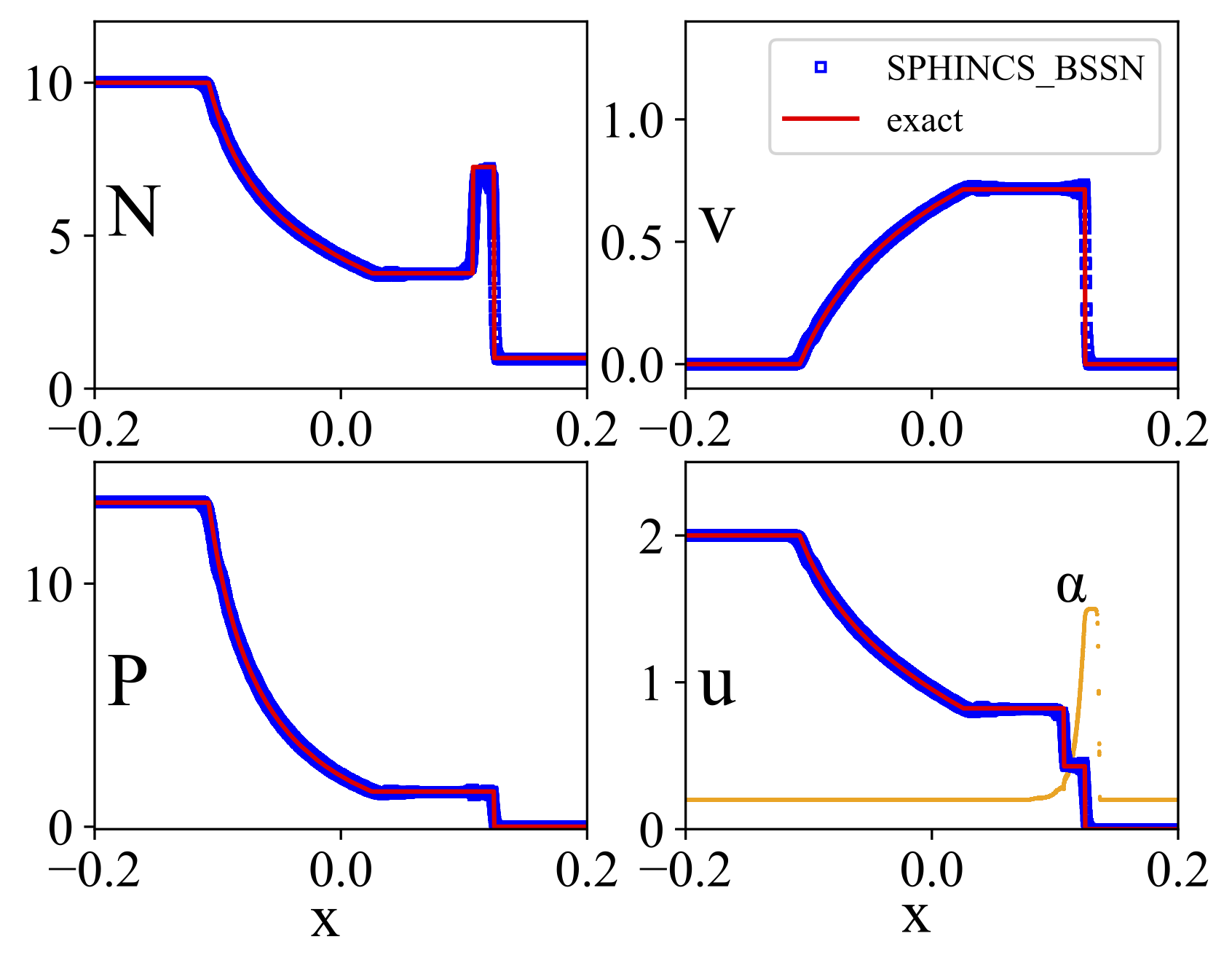
Figure 1: Results for the 3D, relativistic shock tube test. Shown are the result (density, velocity, pressure and internal energy; $\Delta x_{L}=0.00075$) for our default choices, the orange dots in the "u" panel show values of the dissipation parameter $\alpha$. Dissipation robustly switches on ahead of the shock front, remains approximately constant around the shock front and decays quickly in the post-shock region.

3.1 Shock tube

This test is a relativistic version of “Sod’s shocktube” Sod (1978) which has become a standard benchmark for relativistic hydrodynamics codes Marti and Müller (1996); Chow and Monaghan (1997); Siegler and Riffert (2000); Del Zanna and Bucciantini (2002); Marti and Müller (2003, 2015). Apart from demonstrating that our code solves the relativistic hydrodynamics equations correctly, we use this test here also to show where our steering method, see Sec. 2.1.3, triggers dissipation.
The test uses a polytropic exponent $\Gamma=5/3$ and as initial conditions

$$\left[N,P\right]=\left\{\begin{array}[]{ll}\left[10,\frac{40}{3}\right],&{\rm for\;}x<0\\ \\ \left[1,10^{-6}\right]&{\rm for\;}x\geq 0,\end{array}\right.$$ (57)

with velocities initially being zero everywhere. We place particles with equal baryon numbers on close-packed lattices as described in Rosswog (2015), so that on the left side the particle spacing is $\Delta x_{L}=0.00075$ and we have 12 particles in both $y$- and $z$-direction. This test is performed with the full GR-code in a fixed Minkowski metric. The result at $t=0.15$ is shown in Fig. 1 with the SPHINCS_BSSN  results marked with blue squares and the exact solution Marti and Müller (2003) with the red line.
The SPHINCS_BSSN  results (blue squares) are in very good agreement with the exact solution (red line). In the fourth sub-panel we show in orange the dissipation parameter $\alpha$. It abruptly switches to $\alpha^{\rm max}$ just ahead of the shock front, stays constant around it, and decays in the post-shock region very quickly to the floor value. Overall we have a very good agreement with the exact solution. Only directly behind the shock front (e.g. in velocity and density) is a small amount of noise visible. This is to some extent unavoidable, since the particles try to optimize their local distribution, see e.g. Sec. 3.2.3 in Rosswog (2015), and need to transition from their initial arrangement into a new one.
We have also experimented with other slope limiters (van Leer van Leer (1977), vanLeer Monotonized Central van Leer (1977) and superbee Sweby (1984)), but all of them showed an increased velocity overshoot at the shock front and no obvious other advantage. We therefore settled on the minmod limiter, but we do not expect to see substantial differences when other slope limiters are used and this is also confirmed by a number of additional merger test simulations (not discussed further here).
For more special-relativistic benchmark tests with SPH the interested reader is referred to Rosswog (2010, 2011, 2015).

3.2 Binary mergers

3.2.1 Performed simulations

Our performed simulations are summarized in Tab. 3.2.1. We perform for each EOS several runs with at least two different resolutions (1 and 2 million SPH particles; for the grid resolution see below) and for a case where the cold nuclear part corresponds to the MPA1 EOS we also vary the thermal exponent $\gamma_{\rm th}$. For our presumably most realistic EOSs, MPA1 and APR3, we also perform runs with 5 million particles, but we note that these runs are extremely expensive for our current simulation technology and are therefore not run for as long as the other cases. For the very compact stars resulting from the SLy EOS our current resolution may be at the lower end, especially for 1 million case, and the corresponding results should be taken with a grain of salt. This case will be re-assessed in future, better resolved simulations.
For the spacetime evolution we employ seven levels of fixed mesh refinement with the outer boundaries in each coordinate direction at $\approx 2268$ km and 143, 193, 291 grid points in each direction for the 1, 2 and 5 million SPH particle runs. The corresponding resolution lengths of our finest grids, $\Delta_{g}^{\rm min}$, are shown in the fourth column of Tab. 3.2.1. Note that due to the approach chosen in SPHINCS_BSSN, we have the freedom to choose different resolutions for the spacetime and the hydrodynamics. For example, if the spacetime is not too strongly curved, say, for a neutron star with a rather stiff equation of state, we may obtain reasonably accurate results with only a moderate grid resolution. In such cases, we can instead invest the available computational resources in a higher hydrodynamic resolution, i.e. in larger SPH particle numbers. Since all our simulation technology is very new, the relative resolutions are still to some extent a matter of experiment. This is discussed in more detail in Appendix B. The minimum smoothing lengths reached in each simulation, $h_{\rm min}$, are also shown in Tab. 3.2.1 as a measure of the hydrodynamical resolution length. Note that today’s state-of-the-art Eulerian simulations typically have a smaller finest grid length (e.g. Kashyap et al. (2021) use 185 m), but our hydrodynamic resolution length can go substantially below such length scales, see Tab. 3.2.1.

[H] Simulated binary systems. All binaries are irrotational, have twice 1.3 M_⊙ (gravitational mass of each star in the binary system) and the simulations start from an initial separation of 45 km. Unless mentioned otherwise, the thermal exponent $\gamma_{\rm th}=1.75$ is used. $\Delta_{g}^{\rm min}$ refers to the finest grid resolution length, $h_{\rm min}$ is the minimum resolution length (= smoothing length) in the hydrodynamic evolution. name EOS #particles $\Delta_{g}^{\rm min}$ [m] $h_{\rm min}$ [m] comment MPA1_1mio MPA1 $1\times 10^{6}$ 499 188 MPA1_2mio MPA1 $2\times 10^{6}$ 369 172 MPA1_5mio MPA1 $5\times 10^{6}$ 244 117 MPA1_2mio_$\Gamma_{\rm th}1.5$ MPA1 $2\times 10^{6}$ 369 161 $\gamma_{\rm th}=1.5$ MPA1_2mio_$\Gamma_{\rm th}2.0$ MPA1 $2\times 10^{6}$ 369 149 $\gamma_{\rm th}=2.0$ APR3_1mio APR3 $1\times 10^{6}$ 499 145 APR3_2mio APR3 $2\times 10^{6}$ 369 136 APR3_5mio APR3 $5\times 10^{6}$ 244 106 SLy_1mio SLy $1\times 10^{6}$ 499 140 SLy_2mio SLy $2\times 10^{6}$ 369 106 MS1b_1mio MS1b $1\times 10^{6}$ 499 270 MS1b_2mio MS1b $2\times 10^{6}$ 369 222

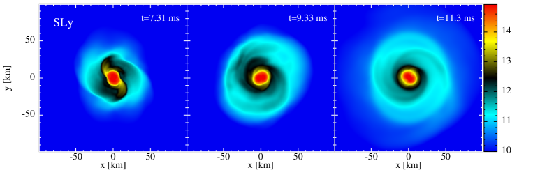
Figure 2: Density evolution (top to bottom row) for the MPA1, APR3, SLy and MS1b EOS. Each time the run with 2 million particles, see Tab. 3.2.1, is shown. For each EOS case, the times are chosen so that they correspond to 1.57, 3.55 and 5.52 ms after merger (defined as the time of peak GW amplitude).

3.2.2 Dynamical evolution

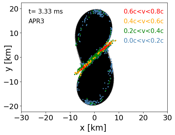
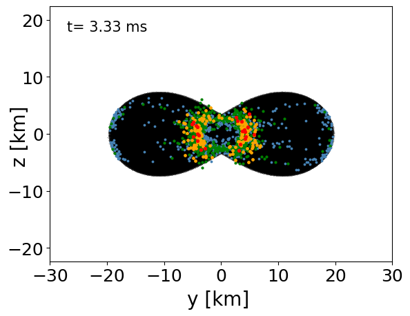
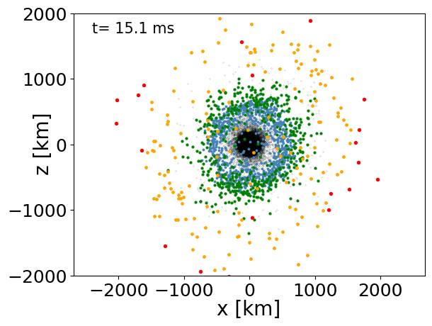
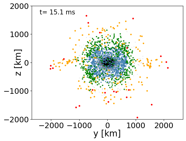
Figure 16: Projections of the particle positions for the APR3 EOS case (run APR3_2mio). All particles are shown in black, ejecta with $v_{\infty}<0.2c$ in blue, ejecta with $0.2c\leq v_{\infty}<0.4c$ in green, ejecta with $0.4c\leq v_{\infty}<0.6c$ in orange and ejecta with $0.6c\leq v_{\infty}<0.8c$ in red.

In Fig. 2 we show the density evolution in the orbital plane for each EOS, every time showing the 2 million particle runs (i.e. for MPA1_2mio, APR3_2mio, SLy_2mio, MS1b_2mio, see Tab. 3.2.1) at 1.57, 3.55 and 5.52 ms after merger (defined as the time of peak GW amplitude). As expected, the EOS has a fair impact on the last inspiral stages where tidal effects accelerate the motion and lead to an earlier merger at lower frequencies as compared to systems without tidal effects (i.e. black hole mergers), see e.g. Flanagan and Hinderer (2008); Damour and Nagar (2010); Bernuzzi (2020).
Our softest EOS, SLy, produces the most compact remnant and undergoes very deep oscillations, see Fig. 3, with the density in the remnant settling to more than twice the initial stellar density. Our two arguably most realistic EOSs, MPA1 and APR3, look morphologically very similar, see the first two rows in Fig. 2, but also their peak density and minimum lapse evolution looks alike: they show a first, dominant compression (density increase $\sim 20-25$%) and then, within a couple of oscillation periods, they settle onto a final central density which is approximately the same as the first compression spike. The extremely stiff MS1b EOS shows a qualitatively similar peak density/lapse evolution, though at substantially lower densities/higher lapse values. Interestingly, none of the explored cases seem close to a collapse to a black hole, even the soft SLy EOS cases settles to a minimum lapse value of $\alpha_{\rm min}\approx 0.35$. As a rule of thumb: systems with central lapses dropping below $\approx 0.2$ are doomed to collapse to a black hole, see, for example, Bernuzzi et al. (2020) or Fig.16 in our first SPHINCS_BSSN  paper Rosswog and Diener (2021) which shows the shape of the lapse function when an apparent horizon is detected for the first time.

Figure 3: Maximum density (in g cm^-3) and minimum lapse value for the runs with 2 million particles (i.e. runs MPA1_2mio, APR3_2mio, SLy_2mio and MS1b_2mio, see Tab. 3.2.1).

We also monitor the quantity $M_{<13}$, the (baryonic) mass of matter with a density smaller than $10^{13}$ g cm^-3 minus the ejected mass, see below, which we consider as a proxy for the resulting torus mass. The astrophysical relevance of the torus mass stems from its role as an energy reservoir for powering short GRBs after the collapse to a BH Nakar (2007); Lee et al. (2009); Kumar and Zhang (2015), but also since $\sim 40$% of this mass can potentially become unbound Metzger et al. (2008); Beloborodov (2008); Siegel and Metzger (2017, 2018); Miller et al. (2019); Fernandez et al. (2019), and therefore likely contributes the lion’s share of the ejecta budget of a neutron star merger.
We show the temporal evolution of $M_{<13}$ in Fig. 4. None of the simulations seems to have reached a stationary state yet, all of them keep shedding mass into the torus, but all have already reached a torus mass exceeding 0.15 M_⊙. Thus, assuming an efficiency $\epsilon$ to translate this rest mass energy reservoir into radiation, bursts with a (true) energy of $>10^{53}\;{\rm erg}\;(\epsilon/0.05)(M_{<13}/0.15M_{\odot})c^{2}$ could be reached. If a fraction of $\eta$ of the initial torus becomes unbound, one can expect neutron-rich ejecta of $>0.06M_{\odot}(\eta/0.4)(M_{<13}/0.15M_{\odot})$, roughly consistent with the estimates for GW170817 Kasen et al. (2017); Cowperthwaite et al. (2017); Evans et al. (2017); Villar et al. (2017); Kasliwal et al. (2017); Tanvir et al. (2017); Rosswog et al. (2018).

Figure 4: Disk mass evolution for the runs with 2 million particles (i.e. runs MPA1_2mio, APR3_2mio, SLy_2mio and MS1b_2mio, see Tab. 3.2.1).

3.2.3 Impact of the thermal index $\gamma_{\rm th}$

Our treatment of thermal effects by adding an ideal gas-type pressure with a thermal index $\gamma_{\rm th}$, see Appendix A, is clearly very simple and recently more sophisticated approaches have been developed Raithel et al. (2019, 2021). In particular, if thermal effects are to be described via such an ideal gas-type index $\gamma_{\rm th}$, it should vary with the local physical conditions (e.g. density). To test for the impact of $\gamma_{\rm th}$, we perform two additional runs (2 $\times 1.3$ M_⊙ with the MPA1 EOS) where we use, apart from our default choice $\gamma_{\rm th}=1.75$, also the values 1.5 and 2.0. The morphology of these runs is shown in Fig. 5. While the impact of $\gamma_{\rm th}$ on the mass distribution is overall moderate, it has some noticeable impact on the spacetime evolution as illustrated with the minimum lapse value shown in Fig. 6, left panel. To get a feeling for the effects of resolution, we plot in the right panel also the MPA1 case for three different resolutions. Smaller values of $\gamma_{\rm th}$ make the EOS overall more compressible which leads to larger amplitude oscillations in the minimum lapse. Since these oscillations go along with mass shedding, there is also some impact of $\gamma_{\rm th}$ on the amount of ejected mass, see below.

Figure 5: Impact of the thermal exponent $\gamma_{\rm th}$ on the evolution. Shown is a binary merger with 2$\times 1.3$ M_⊙, the MPA1 EOS and $\gamma_{\rm th}=1.5$, 1.75 and 2.0 (top to bottom row).

Figure 6: Comparison of the evolution of the minimal lapse value (2$\times 1.3$ M_⊙, MPA1 EOS) for different thermal exponents $\gamma_{\rm th}$ (left) and different resolutions (right).

3.2.4 The triggering of artificial dissipation

To demonstrate where dissipation is triggered in a neutron star merger, we show in Fig. 7 the values of the dissipation parameter $\alpha_{\rm AV}$ for simulation MS1b_2mio. The left panel shows the dissipation parameters at the end of the inspiral, just before merger. At this stage nearly all of the matter has dissipation parameters very close the floor value (here $\alpha_{0}=0.2$), only particles in a thin surface layer (e.g. at the cusps) have moderately larger values. As a side remark, we want to point out how well-behaved the surfaces of the neutron stars are. Contrary to Eulerian hydrodynamics, in our approach no special treatment of the surface layers is needed, the corresponding particles are treated exactly as all the other particles. Inside the stars the dissipation parameter values hardly increase above the floor value, not even during the merger, but the particles that are "squeezed out" of the shear layer between the stars have values $>1$. Since their sound speed drops rapidly during the decompression, their dissipation values only slowly decay towards lower values, see Eq. (29). As mentioned above, we have chosen our dissipation triggers conservatively, so that likely more dissipation is triggered than is actually needed. A possible reduction will be explored in future work.

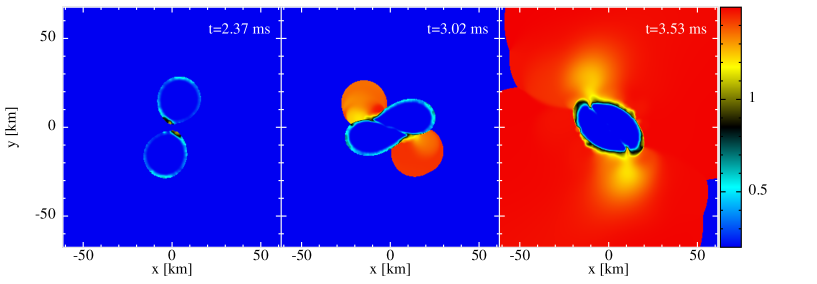
Figure 7: Evolution of the dissipation parameter $\alpha_{\rm AV}$ in simulation MS1b_2mio, see Tab. 3.2.1.

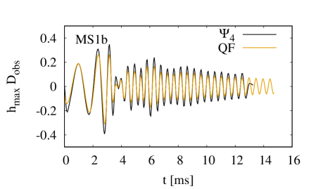
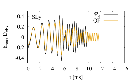
Figure 8: The extracted $\Psi_{4}$ gravitational wave signals for the four different equations of state considered here: MPA1 (top left, MPA1_2mio), APR3 (top right, APR3_2mio), MS1b (bottom left, MS1b_2mio) and SLy (bottom right, SLy_2mio). Both the spacetime-extracted $\Psi_{4}$ (black) and quadrupole (QF; orange) waveforms are shown. The $\Psi_{4}$ waveform has been aligned with the quadrupole waveform by shifting it in time and hence appear to be shorter. The $\Psi_{4}$ waveforms appear to go to zero at the end. This is purely an artifact of the windowing that has been applied for the time integration of $\Psi_{4}$.

3.2.5 Gravitational wave emission

We have extracted gravitational waves from our simulations via the quadrupole formula (using particle information only) as well as directly from the spacetime by calculating the Newman-Penrose Weyl scalar $\Psi_{4}$ (both methods are described in Appendix A in Diener et al. (2022)). After $\Psi_{4}$ (decomposed into spin weight -2 spherical harmonics) is extracted at a coordinate radius of $R=300$, we use built in functionality in kuibit Bozzola (2021) to reconstruct the strain by integrating twice in time (performed in the frequency domain). In order to compare with the waveform extracted with the quadrupole formula, we evaluate the sum of multipoles at the orientation that gives the maximal signal and shift the waveform in time in order to align the peak amplitudes to account for the difference that the $\Psi_{4}$ waveform has to propagate from the source to the detector whereas the quadrupole waveform is extracted at the source.

Figure 9: The extracted $\Psi_{4}$ gravitational wave signals for MPA1 for simulations with 1 million (dashed blue, MPA1_1mio), 2 million (solid orange, MPA1_2mio) and 5 million (solid black, MPA1_5mio) particles. Notice that the 5 million particle simulation has not been run for quite as long as the lower resolution simulations due to its higher computational cost.

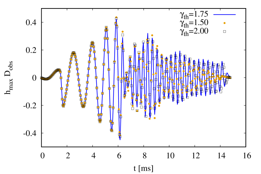
Figure 10: The extracted $\Psi_{4}$ gravitational wave signals for MPA1 with different thermal components $\gamma_{\mathrm{th}}$. Our default, $\gamma_{\mathrm{th}}=1.75$, is shown with a solid blue line, $\gamma_{\mathrm{th}}=1.5$ is shown with orange filled dots and $\gamma_{\mathrm{th}}=2.0$ is shown with black empty squares.

In Fig. 8 we show the extracted gravitational wave signals for the four different equations of state considered here: MPA1 (top left) with thermal component $\gamma_{\mathrm{th}}=1.75$, APR3 (top right), MS1b (bottom left) and SLy (bottom right) extracted from the simulations with 2 million particles. As can be seen the quadrupole formula does a good job in tracking the phase of the waves, but typically underestimates (by up to 60%) the amplitude of the waveform. As mentioned earlier, the larger tidal effects with harder equations of state lead to a faster inspiral and an earlier merger. This is clearly also an effect that is visible in the waveforms, where the SLy (the softest EOS) waveform has a significantly longer inspiral part and the MS1b (the hardest EOS) waveform has the shortest inspiral part. In the post-merger part of the waveform it is also clear that the amplitude of the wave is larger for softer equations of state.
In Fig. 9 we show the extracted gravitational wave signal for MPA1 (with $\gamma_{\mathrm{th}}=1.75$) at 3 different resolutions (1, 2 and 5 million particles). As can be seen, the effect of low resolution (and higher dissipation) is to drive the neutron stars to faster mergers. In addition, there is also a rapid decay in gravitational wave amplitude in the post-merger phase at low resolution. It is clear that we have not quite reached convergence in these simulations even at the highest resolution, but it is encouraging to see that the differences between the two lower resolution simulations are much larger than the differences between the two higher resolutions.
We have checked that the recent changes to the code do not alter the convergence properties in any significant way compared to our recent study Diener et al. (2022). We find that the constraint violation behaviour is virtually identical to what we found there, and we therefore refer the interested reader to Fig. 12 of that study. From that plot the conclusion is that the convergence of the Hamiltonian constraint is consistent with 2nd order.
In Fig. 10 we explore the effect of the different thermal components on the extracted gravitational waveform for the 2 million particle simulations with the MPA1 EOS and $\gamma_{\mathrm{th}}=1.75$, $1.50$ and $2.00$. As expected, the thermal component does not make a difference during the inspiral as the waveforms are practically indistinguishable before the merger. Interestingly, after the merger the softer $\gamma_{\mathrm{th}}=1.5$ simulation shows a significantly faster decay of the gravitational wave signal than the harder ones.
In Fig. 11 we plot the amplitude of the Fourier transform of the dominant $\ell=2,m=2$ mode of the strain as computed from $\Psi_{4}$ for the four different EOS considered here in the left panel, whereas the right panel shows the spectra for the MPA1 EOS with different thermal components. In both plots, the solid lines show the Fourier transforms of the full waveforms, while the dashed lines show the Fourier transforms of the post-merger part of the waveforms only. Consistent with findings reported in the literature Bauswein and Stergioulas (2015); Bernuzzi et al. (2015); Dietrich et al. (2015); Bauswein et al. (2016); Clark et al. (2016); Ciolfi et al. (2017); Maione et al. (2017); Sarin and Lasky (2021); Sun et al. (2022), the spectra at low ($<1$ kHz) frequencies are dominated by the inspiral with increasing amplitude up to a maximum at the frequency of the binary at the merger. This feature is absent in the post-merger spectra. For all the different EOS, the spectra show a dominant peak at higher frequency and the location of that peak is strongly dependent on the EOS. The softer the EOS, the higher the frequency with values ranging from about $2.1$ kHZ for MS1b to $3.4$ kHz for SLy. For the softest EOS (SLy) there is clear evidence of sub-dominant peaks (also reported in the literature) at both lower and higher frequency separated from the dominant peak by about $\pm\Delta f\approx 1$ kHz.
In Table III in Takami et al. (2014) several peak frequencies (in the authors’ convention $f_{\mathrm{max}}$, the instantaneous frequency at maximal GW amplitude, $f_{1}$, the first sub-dominant peak after merger, and $f_{2}$, the dominant peak after merger) are reported for a number of different equations of state and masses of the binary systems. In particular their SLy-q10-M1300 case is very similar to one of our systems (but they use a $\gamma_{\rm th}=2.00$ rather our value of 1.75). Unfortunately, this is our softest equation of state that has the highest resolution requirements and hence is our least trusted case. Nevertheless we find frequencies that are in reasonable agreement. For $f_{1}$ and $f_{2}$ we do see only small differences between the values extracted from our low and medium resolution runs. We find $f_{1}=2.55$ kHz and $f_{2}=3.36$ kHz for 1 million particles and $f_{1}=2.52$ kHZ and $f_{2}=3.39$ kHz for 2 million particles. These are slightly larger than the $f_{1}=2.13$ kHz and $f_{2}=3.23$ kHz values reported in Takami et al. (2014). On the other hand, we do find substantial differences in the value for $f_{\mathrm{max}}$ at the two different values with $f_{\mathrm{max}}=2.14$ kHZ for 1 million particles and $f_{\mathrm{max}}=1.76$ kHz for 2 million particles. This is to be compared with a value of $f_{\mathrm{max}}=1.95$ kHZ in Takami et al. (2014). We suspect that these values are quite sensitive to the details of the inspiral and at current resolutions we still see significant differences for the SLy equation of state. Note that we have not used the fitting procedure described in Takami et al. (2014) to extract the $f_{1}$ and $f_{2}$ frequency peaks, but have simply found the peaks numerically from the raw power spectral density.
Turning now to a comparison of the spectra for MPA1 with different thermal components (right plot), it is clear that there is very little dependence of the location of the dominant peak with $\gamma_{\mathrm{th}}$. However, consistent with the rapid decay of the post-merger waveform for $\gamma_{\mathrm{th}}=1.5$, in Fig. 10 we do see a smaller amplitude of the peak for that case.

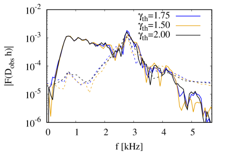
Figure 11: Fourier spectra of the dominant $\ell=2,m=2$ mode of the strain for MPA1 ($\gamma_{\mathrm{th}}=1.75$), APR3, MS1b and SLy (left panel) and for MPA1 ($\gamma_{\mathrm{th}}=1.5,1.75$ and $2.0$) (right panel). In both cases the solid lines shows the spectra of the full waveforms, while the dashed lines show the spectra of the post-merger waveforms only.

3.2.6 Ejecta

The ejection of neutron-rich matter is arguably one of most important aspects of a neutron star merger Rosswog et al. (1999); Freiburghaus et al. (1999); Bauswein et al. (2013); Hotokezaka et al. (2013); Radice et al. (2018), it is responsible for enriching the cosmos with heavy elements and for all of the electromagnetic emission. To identify ejecta, we apply two basic criteria, the "geodesic criterion" and the "Bernoulli criterion", both of which can be augmented by additional conditions (e.g. an outward pointing radial velocity). The geodesic criterion assumes that a fluid element is moving along a geodesic in a time-independent, asymptotically flat spacetime, e.g. Hotokezaka et al. (2013); Foucart et al. (2021). Under these assumptions, $-U_{0}$ corresponds to the Lorentz factor of the fluid element at spatial infinity and therefore a fluid element with

$$-U_{0}>1$$ (58)

is considered as unbound since it still has a finite velocity. In practice however, this criterion ignores potential further acceleration due to internal energy degrees of freedom and we therefore consider the results from the geodesic criterion as a lower limit.
The internal degrees of freedom are included in the Bernoulli criterion, see e.g. Rezzolla and Zanotti (2013), which multiplies the left hand side of the above criterion with the specific enthalpy

$$-\mathcal{E}U_{0}>1.$$ (59)

To avoid falsely identifying hot matter near the centre as unbound, we apply the Bernoulli criterion only to matter outside of a coordinate radius of 100 ($\approx 150$ km). We find very good agreement between both these criteria, with the Bernoulli criterion identifying only a slightly larger amount unbound mass. This is illustrated in Fig. 12 for run APR3_2mio. In the following, we only use the above described version of the Bernoulli criterion.

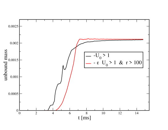
Figure 12: Comparison of the "geodesic" and the (slightly modified) "Bernoulli" criterion to identify unbound mass.

The ejecta mass and average velocities for our runs are summarized in Tab. 3.2.6. Consistent with other studies (e.g. Hotokezaka et al. (2013); Bauswein et al. (2013); Radice et al. (2018)) we find that the studied equal mass systems eject only a few times $10^{-3}$ M_⊙ dynamically, i.e. the dynamical ejecta channel falls short by about an order of magnitude in reproducing the ejecta amounts that have been inferred from GW170817 Kasen et al. (2017); Cowperthwaite et al. (2017); Evans et al. (2017); Villar et al. (2017); Kasliwal et al. (2017); Tanvir et al. (2017); Rosswog et al. (2018). While part of these large inferred masses may be explained by the fact that the interpretations of the observations largely neglect the 3D ejecta geometry and assume sphericity instead Korobkin et al. (2021), it seems obvious that complementary ejecta channels are needed.
Ordering our equations of state in terms of stiffness from soft to hard (either based on $M_{\rm TOV}^{\rm max}$ or $\Lambda_{1.4}$, see Sec. 2.4), SLy, APR3, MPA1, MS1b, we see that they eject more mass the softer they are, consistent with shocks (that emerge easier in soft EOSs with lower sound speed) being the major ejection mechanism and confirming earlier results Bauswein et al. (2013); Hotokezaka et al. (2013). The thermal exponent $\gamma_{\rm th}$ has a noticeable impact on the ejecta masses with the $\gamma_{\rm th}=1.5$ case ejecting nearly twice as much as our standard case. Reference Bauswein et al. (2013) actually finds that ejecta from tabulated EOSs are best approximated by $\gamma_{\rm th}=1.5$, therefore the masses in Tab. 3.2.6 may be considered as lower limits. Given the simplicity of how the thermal contribution is modelled, and its impact on both the GW signal, see Fig. 10, and the ejecta this should also be a warning sign that a more sophisticated modelling of the thermal EOS is needed.
The ejecta velocities in GW170817 have provided additional constraints on the physical origin of the ejecta. Keeping in mind that, within the assumptions entering the Bernoulli criterion, the physical interpretation of $-\mathcal{E}U_{0}$ is that of the Lorentz factor at infinity, we bin the asymptotic velocities

$$v_{\infty}=\sqrt{1-\frac{1}{(\mathcal{E}U_{0})^{2}}}$$ (60)

in Fig. 13. The baryon number weighted average velocities at infinity

$$\langle v_{\infty}\rangle=\frac{\sum_{b}\nu_{b}\;v_{\infty,b}}{\sum_{b}\nu_{b}},$$ (61)

where the index $b$ runs over all unbound particles and $\nu$ is, as before, the baryon number carried by an SPH particle, is typically around $\sim 0.2$ c, but in each of the cases $\sim 10^{-4}$ M_⊙ escapes with velocities above 0.5 c, extending up to $\sim 0.7$ c, see Fig. 13 and Tab. 3.2.6. Such high-velocity ejecta have been reported also by other studies Hotokezaka et al. (2013); Just et al. (2015); Metzger et al. (2015); Radice et al. (2018). While we cannot claim that these small amounts of mass are fully converged, Fig. 14 shows that the velocity distribution in all cases smoothly extends to such large velocity values. We are therefore confident that this high-velocity ejecta component is not a numerical artefact.

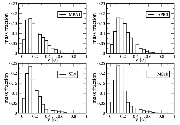
Figure 13: Fraction of the ejected mass binned according to their velocities at infinity, for each equation of state the simulation results with 2 million particles is shown.

[H] Dynamical ejecta masses and velocities of the simulated binary systems. $m_{>Xc}$ refers to the amount of mass that has a velocity in excess of $Xc$. name $m_{\rm ej}$ [$10^{-3}$ M_⊙] $\langle v_{\infty}\rangle[c]$ $m_{>0.5c}$ [M_⊙] $m_{>0.6c}$ [M_⊙] $m_{>0.7c}$ [M_⊙] MPA1_1mio 3.6 0.23 $1.7\times 10^{-4}$ $5.2\times 10^{-5}$ $6.3\times 10^{-6}$ MPA1_2mio 1.6 0.21 $5.6\times 10^{-5}$ $1.1\times 10^{-5}$ 0 MPA1_5mio 1.2 0.24 $1.0\times 10^{-4}$ $3.5\times 10^{-5}$ $3.4\times 10^{-6}$ MPA1_2mio_$\gamma_{\rm th}1.5$ 2.8 0.16 $4.7\times 10^{-5}$ $3.6\times 10^{-6}$ 0 MPA1_2mio_$\gamma_{\rm th}2.0$ 1.8 0.22 $6.9\times 10^{-5}$ $1.7\times 10^{-5}$ $1.0\times 10^{-6}$ APR3_1mio 9.7 0.27 $7.1\times 10^{-4}$ $2.7\times 10^{-4}$ $8.5\times 10^{-5}$ APR3_2mio 2.1 0.22 $9.0\times 10^{-5}$ $2.8\times 10^{-5}$ $4.8\times 10^{-6}$ APR3_5mio 1.9 0.21 $8.3\times 10^{-5}$ $2.0\times 10^{-5}$ $8.4\times 10^{-7}$ SLy_1mio $5.4$ 0.21 $2.7\times 10^{-4}$ $8.4\times 10^{-5}$ $2.1\times 10^{-6}$ SLy_2mio $>6.7$ 0.18 $2.2\times 10^{-4}$ $8.8\times 10^{-5}$ $1.4\times 10^{-5}$ MS1b_1mio 2.9 0.16 $1.1\times 10^{-4}$ $2.8\times 10^{-5}$ 0 MS1b_2mio 2.7 0.18 $8.8\times 10^{-5}$ $3.5\times 10^{-5}$ $5.0\times 10^{-6}$

Figure 14: Asymptotic velocities as a function of radius of the 2 million particle simulations.

To identify how the high-velocity ejecta are launched, we sort the ejecta in the last data output in four groups: $\mathcal{G}_{1}$: $v_{\infty}<0.2c$, $\mathcal{G}_{2}$: $0.2c\leq v_{\infty}<0.4c$, $\mathcal{G}_{3}$: $0.4c\leq v_{\infty}<0.6c$ and $\mathcal{G}_{4}$: $0.6c\leq v_{\infty}<0.8c$. In Figs. 15 to 18 we plot these groups of particles at the approximate times of the merger and for the final data dumps of our 2 million particle runs. The highest velocity particles, $\mathcal{G}_{3}$ (orange) and $\mathcal{G}_{4}$ (red) emerge from the shock-heated interface between the two neutron stars. While the high-velocity ejecta are still not well-resolved, we note that our simulations here have an order of magnitude more particles than the approximate GR simulations in which these fast ejecta were originally identified Metzger et al. (2015). This high-velocity component could have important observational consequences: it may produce an early blue/UV transient on a time scale of several minutes to an hour preceeding the main kilonova event Metzger et al. (2015) and, at late times, it may be responsible for synchrotron emission Mooley et al. (2018); Hotokezaka et al. (2018); Hajela et al. (2022).
Another interesting result in a multi-messenger context is that the ejecta distribution only shows moderate deviations from spherical symmetry, so that the resulting electromagnetic emission could be reasonably modelled with simple approaches. This result, however, may be specific for our equal mass binaries and for the currently implemented physics and it is possible that different equations of state, neutrinos and/or magnetic fields could modify this.

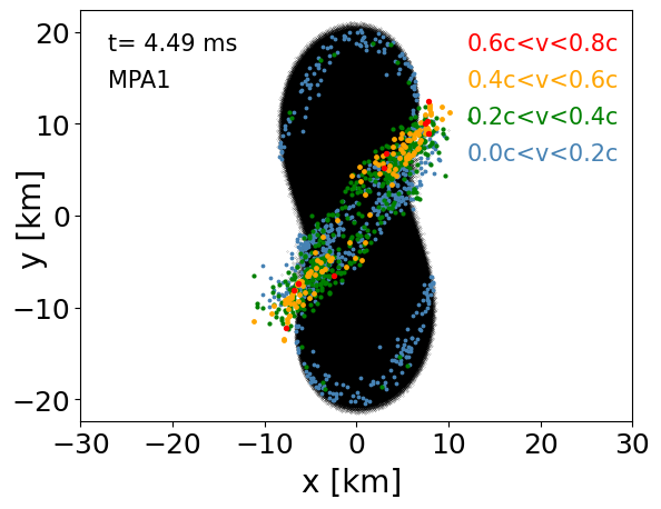
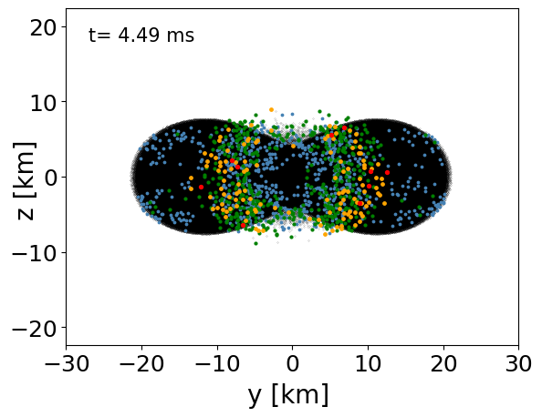
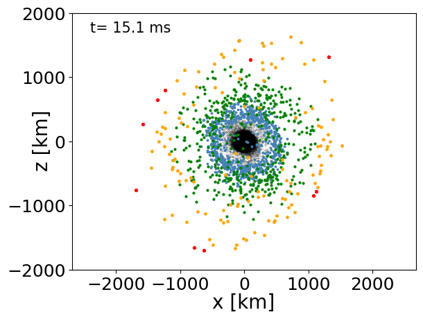
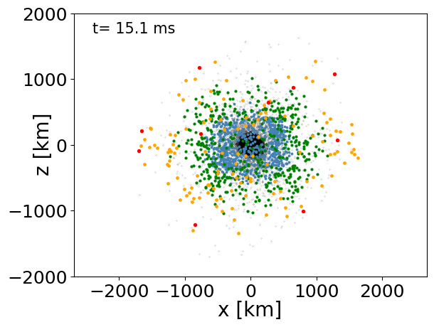
Figure 15: Projections of the particle positions for the MPA1 EOS case (run MPA1_2mio). All particles are shown in black, ejecta with $v_{\infty}<0.2c$ in blue, ejecta with $0.2c\leq v_{\infty}<0.4c$ in green, ejecta with $0.4c\leq v_{\infty}<0.6c$ in orange and ejecta with $0.6c\leq v_{\infty}<0.8c$ in red.

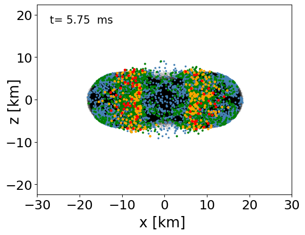
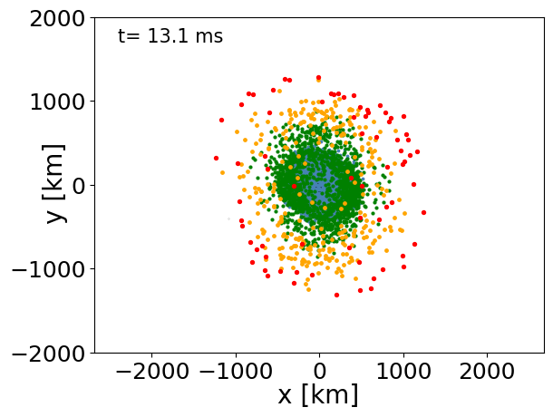
Figure 17: Projections of the particle positions for the SLy EOS case (run SLy_2mio). All particles are shown in black, ejecta with $v_{\infty}<0.2c$ in blue, ejecta with $0.2c\leq v_{\infty}<0.4c$ in green, ejecta with $0.4c\leq v_{\infty}<0.6c$ in orange and ejecta with $0.6c\leq v_{\infty}<0.8c$ in red.

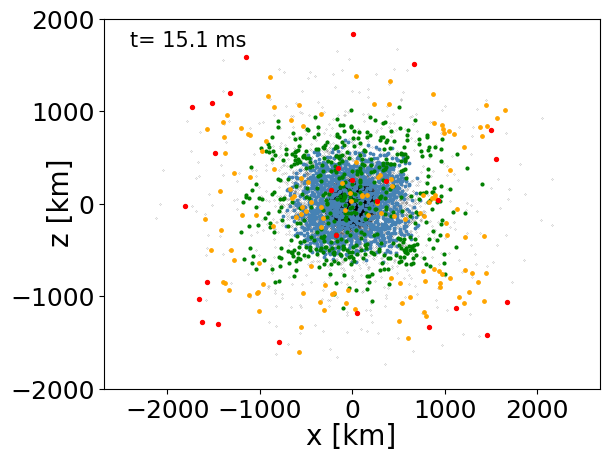
Figure 18: Projections of the particle positions for the Ms1b EOS case (run Ms1b_2mio). All particles are shown in black, ejecta with $v_{\infty}<0.2c$ in blue, ejecta with $0.2c\leq v_{\infty}<0.4c$ in green, ejecta with $0.4c\leq v_{\infty}<0.6c$ in orange and ejecta with $0.6c\leq v_{\infty}<0.8c$ in red.

4 Summary

We have presented here a further methodological refinement of our Lagrangian Numerical Relativity code SPHINCS_BSSN  Rosswog and Diener (2021); Diener et al. (2022). The new methodological elements in SPHINCS_BSSN  include a new way to steer where artificial dissipation is applied, see Sec. 2.1.1. We use both a compression that increases in time (as suggested in Cullen and Dehnen (2010)) and a numerical noise indicator following Rosswog (2015) to determine how much dissipation is used. We have also further refined our MOOD algorithm that we use in our "particle-to-mesh" step, see Sec. 2.3. As a step towards more realistic neutron star merger simulations, we have implemented piecewise polytropic equations of state that approximate the cold nuclear matter equations of state MPA1, APR3, SLy and MS1b and we have augmented these with a thermal contribution, see Sec. 2.4 and Appendix A for details.
In this first SPHINCS_BSSN  study using piecewise polytropic EOSs, we have restricted ourselves to neutron star binary systems with 2 $\times$ 1.3 M_⊙ and we have explored how the results depend on both resolution and the choice of the thermal polytropic exponent $\gamma_{\rm th}$. None of the explored cases seems to be prone to a BH collapse, at least not on the simulated time scale of $\sim 15$ ms. But the SLy EOS cases undergo particularly deep pulsations during which they shed mass into the surrounding torus and they also eject more mass than the stiffer equations of state (MPA1,APR3, MS1b). When our simulations end, the remnant has not yet settled into a stationary state and the torus mass is still increasing. All of the torus masses are large enough to power short GRBs and, if indeed tori unbind several 10% of their mass on secular time scales Metzger et al. (2008); Beloborodov (2008); Siegel and Metzger (2017, 2018); Miller et al. (2019); Fernandez et al. (2019), then in all cases their ejecta amount to a few percent of a solar mass.
For all our runs we extract the gravitational waves, both directly from the particles via the quadrupole approximation and from the spacetime by means of the Newman-Penrose Weyl scalar $\Psi_{4}$. Overall, we find rather good agreement, the waves phases are practically perfectly tracked in the quadrupole approximation, but in the post-merger phase the amplitudes can be underestimated by several 10%. As expected, the softest EOS leads to the longest inspiral wave train and also to larger post-merger amplitudes. We further explore the impact of the thermal adiabatic exponent $\gamma_{\rm th}$ on the gravitational wave and spectrum.
Consistent with earlier studies, we find that these equal mass systems eject only a few $10^{-3}$ M_⊙ dynamically and the ejection is driven by shocks. Based on quasi-Newtonian Rosswog et al. (1999, 2000); Korobkin et al. (2012); Rosswog (2013), conformal flatness approximation Bauswein et al. (2013) and full-GR simulations Hotokezaka et al. (2013); Radice et al. (2018), however, we expect that asymmetric systems with mass ratio $q\neq 1$ eject substantially more matter and in particular have a larger contribution from tidal ejecta. Overall, the small amount of ejecta underlines the need for additional ejection channels such as torus unbinding or neutrino-driven winds in order to reach the ejecta masses estimated for GW170817. The matter being predominantly ejected via shocks probably means that its electron fraction is increased with respect to the cold, $\beta$-equilibrium values inside the original neutron stars ($\sim 0.05$, see e.g. Fig. 21 in Farouqi et al. (2021)). Again consistent with earlier studies, we find that the softer equation of state cases eject more mass and also reducing the exponent $\gamma_{\rm th}$ seems to enhance mass ejection.
Interestingly, we find in all cases that $\sim 10^{-4}$ M_⊙ are escaping at velocities exceeding 0.5c and this high-velocity part of the ejecta originates from the interface between the two neutron stars during merger. While we cannot claim that the properties of this matter are well converged, we see this fast component in all the simulations and their velocity distribution, see Fig. 14, extends smoothly to large velocities, so that we have confidence in the physical presence of these high-velocity ejecta. This neutron-rich matter expands sufficiently fast for most neutrons to avoid capture and the $\beta$-decay of these free neutrons has been discussed as a source of early, blue "precursor" emission before the main kilonova Metzger et al. (2015). To "bracket" the kilonova emission, such a high-velocity ejecta component has also been suggested to be responsible for a X-ray emission excess observed three years after GW170817 Hajela et al. (2022).
While the piecewise polytropic equations of state are an important improvement over our previous merger simulations with SPHINCS_BSSN  Diener et al. (2022), they are still only a far cry from realistic microphysics. This topic is a major target for our future work.

SR has been supported by the Swedish Research Council (VR) under grant number 2020-05044, by the Swedish National Space Board under grant number Dnr. 107/16, by the research environment grant “Gravitational Radiation and Electromagnetic Astrophysical Transients (GREAT)” funded by the Swedish Research Council (VR) under Dnr 2016-06012, by which also FT is supported, and by the Knut and Alice Wallenberg Foundation under grant Dnr. KAW 2019.0112.

Appendix A Recovery procedure for piecewise polytropic equations of state

In this work we use piecewise polytropic equations of state. The part resulting from the cold, nuclear matter pressure $P_{\rm cold}$ is described by several polytropic pieces as discussed in Read et al. (2009), and a thermal part, $P_{\rm th}$, is added under the assumption that it also follows a polytropic equation of state with some thermal exponent $\gamma_{\rm th}$, for which we choose a default value of 1.75. The total pressure is then given by

$$P=P_{\rm cold}+P_{\rm th},$$ (62)

where the cold part is given by pieces

$$P_{\rm cold}=K_{i}\rho^{\gamma_{i}},$$ (63)

where the values $\{K_{i},\gamma_{i}\}$ are chosen according to the density (for $\rho_{i}\leq\rho<\rho_{i+1}$). The thermal pressure is calculated only from the "thermal" (i.e. non-degenerate) part of the internal energy and has a separate (smaller) polytropic exponent

$$P_{\rm th}=(\gamma_{\rm th}-1)\rho u_{\rm th}.$$ (64)

The thermal part of $u$ is found by subtracting the "cold/degenerate" value of the internal energy. This cold value is

$$u_{\rm cold}=a_{i}+\frac{K_{i}}{\gamma_{i}-1}\rho^{\gamma_{i}-1}$$ (65)

and the integration constants $a_{i}$ make the internal energy continuous between different pieces, see Eq.(7) of Read et al. (2009).
From now onwards, we will again use our conventions and measure energies in units of $m_{0}c^{2}$, $m_{0}$ being the baryon mass, so that our pressure is given as $P=(\gamma-1)\,n\,u$. The general strategy is similar to the purely polytropic case: we express both $n$ and $u$ in terms of $S_{i}$, $e$, $N$ and the pressure, substitute everything into the (here analytically known) equation of state

$$f(P) \equiv P-(P_{\rm cold}+P_{\rm th})$$ (66)

$$= P-\left\{K_{i}n^{\gamma_{i}}+(\gamma_{\rm th}-1)n\left[u-a_{i}-\frac{K_{i}}{\gamma_{i}-1}n^{\gamma_{i}-1}\right]\right\}=0.$$

and solve numerically for the new pressure that is consistent with the current values of $S_{i}$, $e$ and $N$. We need

$$n=n(S_{i},e,N,P)\quad{\rm and}\quad u=u(S_{i},e,N,P).$$ (67)

We find that the generalized Lorentz factor $\Theta$ can be expressed as

$$\Theta(S_{i},e,N,P)=\sqrt{\frac{-g^{00}}{1+\frac{A}{B^{2}}}},$$ (68)

where

$$A\equiv g^{00}g^{jk}S_{j}S_{k}-(g^{0j}S_{j})^{2}\quad{\rm and}\quad B\equiv g^{0j}S_{j}-g^{00}\left(\frac{\sqrt{-g}}{N}P+e\right).$$ (69)

This provides us with the internal energy

$$u(S_{i},e,N,P)=\frac{g^{0j}S_{j}}{\Theta}-\frac{g^{00}e}{\Theta}-\frac{\sqrt{-g}P}{\Theta N}\left(g^{00}+\Theta^{2}\right)-1.$$ (70)

and, from our earlier definition, we have

$$n(S_{i},e,N,P)=\frac{N}{\sqrt{-g}\Theta}.$$ (71)

The solution procedure is then the following. We first find the new pressure that fulfills Eq. (66) for the new values of $S_{i},e,N$. For this root finding we use Ridders’ method Ridders (1982); Press et al. (1992). This method is a robust variant of the regula falsi method and does not require any derivates. With the consistent pressure at hand, we obtain the new $\Theta$ from Eq. (68). It can be shown that

$$\Theta\mathcal{E}=g^{0j}S_{j}-g^{00}\left(\frac{\sqrt{-g}P}{N}+e\right),$$ (72)

and this provides us with the enthalpy $\mathcal{E}$ and the covariant spatial velocity components $v_{i}=S_{i}/(\Theta\mathcal{E}).$ The time component is found from the equation for the generalized Lorentz factor, Eq.(2),

$$v_{0}=\frac{1-g^{0i}v_{i}}{g^{00}}.$$ (73)

The contravariant velocity is then straight-forwardly calculated via $v^{i}=g^{i\lambda}v_{\lambda}$, $n$ from Eq. (71) and the internal energy as $u=\mathcal{E}-\frac{P}{n}-1$.

Appendix B Which resolution?

In our new simulation methodology, where we evolve the spacetime on a mesh and the matter with particles, we have two different resolution lengths and it its not a priori clear how they should be related. We therefore present here some numerical experiments to shed some light on the effects of the grid- and particle resolution. To keep the parameter space under control, we restrict ourselves here to one of our "most realistic" equations of state, MPA1. We perform the following test simulations:

• TS1: the outer boundary in each coordinate direction is located at 375 ($\approx 554$ km), five refinement levels and $175^{3}$ grid points which corresponds to the finest grid resolution length of $\Delta_{\rm g}^{\rm min}\approx 400$ m. We use here our default, i.e. 6th order, Finite Differencing ("FD6").

• TS2: same as TS1, but FD4

• TS3: same as TS1, but FD8

• TS4: same as TS1, but $233^{3}$ grid points, i.e. $\Delta_{\rm g}^{\rm min}\approx 300$ m

• TS5: same as TS1, but $351^{3}$ grid points, i.e. $\Delta_{\rm g}^{\rm min}\approx 200$ m.

• TS6: same as TS1, but $401^{3}$ grid points, i.e. $\Delta_{\rm g}^{\rm min}\approx 175$ m.

All the variations related to the spacetime evolution accuracy indicate that the changes in the inspiral are only minor and our default of 175³ grid points together with 6th order finite differencing is a good choice.

Figure 19: Dependence of the inspiral on the grid resolution (left) and Finite Differencing order (right). The length labels in the left panel refer to the finest grid resolution $\Delta_{\rm g}^{\rm min}$.

Given that spacetime resolution has only a very minor impact on the inspiral, but we still see substantial difference between the 2 million and the 5 million particle run in Fig.  9, this suggests that it is the particle number that, at the available resolutions, has the largest impact. While we currently have no accurate estimate for the number of particles that is required for a fully converged inspiral, Fig.  9 seems to indicate that we need at least $\sim$ 5 million particles, but possibly more. This issue will be explored in more detail in future work.

References

yes

References

- Abbott et al. (2021) Abbott, R.; Abbott, T.D.; Abraham, S.; Acernese, F.; Ackley, K.; Adams, A.; Adams, C.; Adhikari, R.X.; Adya, V.B.; Affeldt, C.; Agathos, M.; Agatsuma, K.; Aggarwal, N.; Aguiar, O.D.; Aiello, L.; Ain, A.; Ajith, P.; Akcay, S.; Allen, G.; Allocca, A.; Altin, P.A.; Amato, A.; Anand, S.; Ananyeva, A.; Anderson, S.B.; Anderson, W.G.; Angelova, S.V.; Ansoldi, S.; Antelis, J.M.; Antier, S.; Appert, S.; Arai, K.; Araya, M.C.; Areeda, J.S.; Arène, M.; Arnaud, N.; Aronson, S.M.; Arun, K.G.; Asali, Y.; Ascenzi, S.; Ashton, G.; Aston, S.M.; Astone, P.; Aubin, F.; Aufmuth, P.; AultONeal, K.; Austin, C.; Avendano, V.; Babak, S.; Badaracco, F.; Bader, M.K.M.; Bae, S.; Baer, A.M.; Bagnasco, S.; Baird, J.; Ball, M.; Ballardin, G.; Ballmer, S.W.; Bals, A.; Balsamo, A.; Baltus, G.; Banagiri, S.; Bankar, D.; Bankar, R.S.; Barayoga, J.C.; Barbieri, C.; Barish, B.C.; Barker, D.; Barneo, P.; Barnum, S.; Barone, F.; Barr, B.; Barsotti, L.; Barsuglia, M.; Barta, D.; Bartlett, J.; Bartos, I.; Bassiri, R.; Basti, A.; Bawaj, M.; Bayley, J.C.; Bazzan, M.; Becher, B.R.; Bécsy, B.; Bedakihale, V.M.; Bejger, M.; Belahcene, I.; Beniwal, D.; Benjamin, M.G.; Bennett, T.F.; Bentley, J.D.; Bergamin, F.; Berger, B.K.; Bergmann, G.; Bernuzzi, S.; Berry, C.P.L.; Bersanetti, D.; Bertolini, A.; Betzwieser, J.; Bhandare, R.; .; LIGO Scientific Collaboration.; Virgo Collaboration. GWTC-2: Compact Binary Coalescences Observed by LIGO and Virgo during the First Half of the Third Observing Run. Physical Review X 2021, 11, 021053, [arXiv:gr-qc/2010.14527]. doi:\changeurlcolorblack10.1103/PhysRevX.11.021053.
- Baiotti (2019) Baiotti, L. Gravitational waves from neutron star mergers and their relation to the nuclear equation of state. Progress in Particle and Nuclear Physics 2019, 109, 103714, [arXiv:astro-ph.HE/1907.08534]. doi:\changeurlcolorblack10.1016/j.ppnp.2019.103714.
- Ruffert et al. (1997) Ruffert, M.; Janka, H.; Takahashi, K.; Schaefer, G. Coalescing neutron stars - a step towards physical models. II. Neutrino emission, neutron tori, and gamma-ray bursts. A & A 1997, 319, 122–153.
- Rosswog and Liebendörfer (2003) Rosswog, S.; Liebendörfer, M. High-resolution calculations of merging neutron stars - II. Neutrino emission. MNRAS 2003, 342, 673–689. doi:\changeurlcolorblack10.1046/j.1365-8711.2003.06579.x.
- Sekiguchi et al. (2011) Sekiguchi, Y.; Kiuchi, K.; Kyutoku, K.; Shibata, M. Gravitational Waves and Neutrino Emission from the Merger of Binary Neutron Stars. Physical Review Letters 2011, 107, 051102, [arXiv:gr-qc/1105.2125]. doi:\changeurlcolorblack10.1103/PhysRevLett.107.051102.
- Perego et al. (2014) Perego, A.; Rosswog, S.; Cabezón, R.M.; Korobkin, O.; Käppeli, R.; Arcones, A.; Liebendörfer, M. Neutrino-driven winds from neutron star merger remnants. MNRAS 2014, 443, 3134–3156. doi:\changeurlcolorblack10.1093/mnras/stu1352.
- Just et al. (2015) Just, O.; Bauswein, A.; Pulpillo, R.A.; Goriely, S.; Janka, H.T. Comprehensive nucleosynthesis analysis for ejecta of compact binary mergers. MNRAS 2015, 448, 541–567, [arXiv:astro-ph.SR/1406.2687]. doi:\changeurlcolorblack10.1093/mnras/stv009.
- Fujibayashi et al. (2020) Fujibayashi, S.; Shibata, M.; Wanajo, S.; Kiuchi, K.; Kyutoku, K.; Sekiguchi, Y. Mass ejection from disks surrounding a low-mass black hole: Viscous neutrino-radiation hydrodynamics simulation in full general relativity. Phys. Rev. D 2020, 101, 083029, [arXiv:astro-ph.HE/2001.04467]. doi:\changeurlcolorblack10.1103/PhysRevD.101.083029.
- Foucart et al. (2021) Foucart, F.; Duez, M.D.; Hébert, F.; Kidder, L.E.; Kovarik, P.; Pfeiffer, H.P.; Scheel, M.A. Implementation of Monte Carlo Transport in the General Relativistic SpEC Code. ApJ 2021, 920, 82, [arXiv:astro-ph.HE/2103.16588]. doi:\changeurlcolorblack10.3847/1538-4357/ac1737.
- Just et al. (2022) Just, O.; Goriely, S.; Janka, H.T.; Nagataki, S.; Bauswein, A. Neutrino absorption and other physics dependencies in neutrino-cooled black hole accretion discs. MNRAS 2022, 509, 1377–1412, [arXiv:astro-ph.HE/2102.08387]. doi:\changeurlcolorblack10.1093/mnras/stab2861.
- Radice et al. (2022) Radice, D.; Bernuzzi, S.; Perego, A.; Haas, R. A New Moment-Based General-Relativistic Neutrino-Radiation Transport Code: Methods and First Applications to Neutron Star Mergers. MNRAS 2022, [arXiv:astro-ph.HE/2111.14858]. doi:\changeurlcolorblack10.1093/mnras/stac589.
- Price and Rosswog (2006) Price, D.; Rosswog, S. Producing ultra-strong magnetic fields in neutron star mergers. Science 2006, 312, 719.
- Kiuchi et al. (2015) Kiuchi, K.; Cerdá-Durán, P.; Kyutoku, K.; Sekiguchi, Y.; Shibata, M. Efficient magnetic-field amplification due to the Kelvin-Helmholtz instability in binary neutron star mergers. Phys. Rev. D 2015, 92, 124034, [arXiv:astro-ph.HE/1509.09205]. doi:\changeurlcolorblack10.1103/PhysRevD.92.124034.
- Palenzuela et al. (2015) Palenzuela, C.; Liebling, S.L.; Neilsen, D.; Lehner, L.; Caballero, O.L.; O’Connor, E.; Anderson, M. Effects of the microphysical equation of state in the mergers of magnetized neutron stars with neutrino cooling. Phys. Rev. D 2015, 92, 044045, [arXiv:gr-qc/1505.01607]. doi:\changeurlcolorblack10.1103/PhysRevD.92.044045.
- Rosswog and Diener (2021) Rosswog, S.; Diener, P. SPHINCS_BSSN: a general relativistic smooth particle hydrodynamics code for dynamical spacetimes. Classical and Quantum Gravity 2021, 38, 115002, [arXiv:gr-qc/2012.13954]. doi:\changeurlcolorblack10.1088/1361-6382/abee65.
- Diener et al. (2022) Diener, P.; Rosswog, S.; Torsello, F. Simulating neutron star mergers with the Lagrangian Numerical Relativity code SPHINCS_BSSN. European Physical Journal A 2022, 58, 74, [arXiv:astro-ph.HE/2203.06478]. doi:\changeurlcolorblack10.1140/epja/s10050-022-00725-7.
- Shibata and Nakamura (1995) Shibata, M.; Nakamura, T. Evolution of three-dimensional gravitational waves: Harmonic slicing case. Phys. Rev. D 1995, 52, 5428–5444. doi:\changeurlcolorblack10.1103/PhysRevD.52.5428.
- Baumgarte and Shapiro (1999) Baumgarte, T.W.; Shapiro, S.L. Numerical integration of Einstein’s field equations. Phys. Rev. D 1999, 59, 024007, [arXiv:gr-qc/9810065]. doi:\changeurlcolorblack10.1103/PhysRevD.59.024007.
- Rosswog et al. (1999) Rosswog, S.; Liebendörfer, M.; Thielemann, F.K.; Davies, M.; Benz, W.; Piran, T. Mass ejection in neutron star mergers. A & A 1999, 341, 499–526.
- Oechslin and Janka (2007) Oechslin, R.; Janka, H. Gravitational Waves from Relativistic Neutron-Star Mergers with Microphysical Equations of State. Physical Review Letters 2007, 99, 121102, [arXiv:astro-ph/0702228]. doi:\changeurlcolorblack10.1103/PhysRevLett.99.121102.
- Bauswein et al. (2013) Bauswein, A.; Goriely, S.; Janka, H.T. Systematics of Dynamical Mass Ejection, Nucleosynthesis, and Radioactively Powered Electromagnetic Signals from Neutron-star Mergers. ApJ 2013, 773, 78. doi:\changeurlcolorblack10.1088/0004-637X/773/1/78.
- Hotokezaka et al. (2013) Hotokezaka, K.; Kiuchi, K.; Kyutoku, K.; Okawa, H.; Sekiguchi, Y.i.; Shibata, M.; Taniguchi, K. Mass ejection from the merger of binary neutron stars. Phys. Rev. D 2013, 87, 024001. doi:\changeurlcolorblack10.1103/PhysRevD.87.024001.
- Radice et al. (2018) Radice, D.; Perego, A.; Hotokezaka, K.; Fromm, S.A.; Bernuzzi, S.; Roberts, L.F. Binary Neutron Star Mergers: Mass Ejection, Electromagnetic Counterparts, and Nucleosynthesis. ApJ 2018, 869, 130, [arXiv:astro-ph.HE/1809.11161]. doi:\changeurlcolorblack10.3847/1538-4357/aaf054.
- Schoepe et al. (2018) Schoepe, A.; Hilditch, D.; Bugner, M. Revisiting hyperbolicity of relativistic fluids. Phys. Rev. D 2018, 97, 123009, [arXiv:gr-qc/1712.09837]. doi:\changeurlcolorblack10.1103/PhysRevD.97.123009.
- Rosswog (2020) Rosswog, S. The Lagrangian hydrodynamics code MAGMA2. MNRAS 2020, 498, 4230–4255, [arXiv:astro-ph.IM/1911.13093]. doi:\changeurlcolorblack10.1093/mnras/staa2591.
- (26) LORENE library. https://lorene.obspm.fr.
- Read et al. (2009) Read, J.S.; Lackey, B.D.; Owen, B.J.; Friedman, J.L. Constraints on a phenomenologically parametrized neutron-star equation of state. Phys. Rev. D 2009, 79, 124032, [arXiv:astro-ph/0812.2163]. doi:\changeurlcolorblack10.1103/PhysRevD.79.124032.
- Cullen and Dehnen (2010) Cullen, L.; Dehnen, W. Inviscid smoothed particle hydrodynamics. MNRAS 2010, 408, 669–683, [arXiv:astro-ph.IM/1006.1524]. doi:\changeurlcolorblack10.1111/j.1365-2966.2010.17158.x.
- Rosswog (2015) Rosswog, S. Boosting the accuracy of SPH techniques: Newtonian and special-relativistic tests. MNRAS 2015, 448, 3628–3664, [arXiv:astro-ph.IM/1405.6034]. doi:\changeurlcolorblack10.1093/mnras/stv225.
- Rosswog (2009) Rosswog, S. Astrophysical Smooth Particle Hydrodynamics. New Astronomy Reviews 2009, 53, 78–104.
- Rosswog (2020) Rosswog, S. A Simple, Entropy-based Dissipation Trigger for SPH. ApJ 2020, 898, 60, [arXiv:astro-ph.IM/1912.01095]. doi:\changeurlcolorblack10.3847/1538-4357/ab9a2e.
- Alcubierre (2008) Alcubierre, M. Introduction to 3+1 Numerical Relativity; Oxford University Press, 2008.
- Baumgarte and Shapiro (2010) Baumgarte, T.W.; Shapiro, S.L. Numerical Relativity: Solving Einstein’s Equations on the Computer; 2010.
- Rezzolla and Zanotti (2013) Rezzolla, L.; Zanotti, O. Relativistic Hydrodynamics; 2013.
- Shibata (2016) Shibata, M. Numerical Relativity; 2016. doi:\changeurlcolorblack10.1142/9692.
- Wendland (1995) Wendland, H. Piecewise polynomial, positive definite and compactly supported radial functions of minimal degree. Advances in Computational Mathematics 1995, 4, 389–296.
- Gafton and Rosswog (2011) Gafton, E.; Rosswog, S. A fast recursive coordinate bisection tree for neighbour search and gravity. MNRAS 2011, 418, 770–781, [arXiv:astro-ph.IM/1108.0028]. doi:\changeurlcolorblack10.1111/j.1365-2966.2011.19528.x.
- Laguna et al. (1993) Laguna, P.; Miller, W.A.; Zurek, W.H. Smoothed particle hydrodynamics near a black hole. ApJ 1993, 404, 678–685. doi:\changeurlcolorblack10.1086/172321.
- von Neumann and Richtmyer (1950) von Neumann, J.; Richtmyer, R.D. A Method for the Numerical Calculation of Hydrodynamic Shocks. Journal of Applied Physics 1950, 21, 232–237.
- Liptai and Price (2019) Liptai, D.; Price, D.J. General relativistic smoothed particle hydrodynamics. MNRAS 2019, 485, 819–842, [arXiv:astro-ph.IM/1901.08064]. doi:\changeurlcolorblack10.1093/mnras/stz111.
- Christensen (1990) Christensen, R.B. Godunov methods on a staggered mesh–an improved artificial viscosity. Nuclear Explosives Code Developers Conference, volume UCRL-JC-105269. Lawrence Livermore National Lab, Lawrence Livermore Technical Report. 1990, UCRL-JC-105269.
- Frontiere et al. (2017) Frontiere, N.; Raskin, C.D.; Owen, J.M. CRKSPH - A Conservative Reproducing Kernel Smoothed Particle Hydrodynamics Scheme. Journal of Computational Physics 2017, 332, 160–209, [arXiv:physics.comp-ph/1605.00725]. doi:\changeurlcolorblack10.1016/j.jcp.2016.12.004.
- Brown et al. (2009) Brown, J.D.; Diener, P.; Sarbach, O.; Schnetter, E.; Tiglio, M. Turduckening black holes: an analytical and computational study. Phys. Rev. D 2009, 79, 044023, [arXiv:0809.3533 [gr-qc]].
- Einstein Toolkit web page (2020) Einstein Toolkit web page. https://einsteintoolkit.org/, 2020. [Online; accessed 9-December-2020].
- Löffler et al. (2012) Löffler, F.; Faber, J.; Bentivegna, E.; Bode, T.; Diener, P.; Haas, R.; Hinder, I.; Mundim, B.C.; Ott, C.D.; Schnetter, E.; Allen, G.; Campanelli, M.; Laguna, P. The Einstein Toolkit: A Community Computational Infrastructure for Relativistic Astrophysics. Class. Quantum Grav. 2012, 29, 115001, [arXiv:1111.3344 [gr-qc]]. doi:\changeurlcolorblackdoi:10.1088/0264-9381/29/11/115001.
- Cottet and Koumoutsakos (2000) Cottet, G.H.; Koumoutsakos, P.D. Vortex Methods; 2000.
- Cottet et al. (2014) Cottet, G.; Etancelin, J.; Perignon, F.; Picard, C. High order Semi-Lagrangian particle methods for tranport equations. ESAIM: Mathematical Modelling and Numerical Analysis, EDP Sciences 2014, 48, 1029 – 1060. doi:\changeurlcolorblack10.1086/185939.
- Douchin and Haensel (2001) Douchin, F.; Haensel, P. A unified equation of state of dense matter and neutron star structure. A & A 2001, 380, 151–167, [arXiv:astro-ph/astro-ph/0111092]. doi:\changeurlcolorblack10.1051/0004-6361:20011402.
- Akmal et al. (1998) Akmal, A.; Pandharipande, V.R.; Ravenhall, D.G. Equation of state of nucleon matter and neutron star structure. Phys. Rev. C 1998, 58, 1804–1828, [hep-ph/9804388]. doi:\changeurlcolorblack10.1103/PhysRevC.58.1804.
- Müther et al. (1987) Müther, H.; Prakash, M.; Ainsworth, T.L. The nuclear symmetry energy in relativistic Brueckner-Hartree-Fock calculations. Physics Letters B 1987, 199, 469–474. doi:\changeurlcolorblack10.1016/0370-2693(87)91611-X.
- Müller and Serot (1996) Müller, H.; Serot, B.D. Relativistic mean-field theory and the high-density nuclear equation of state. Nuc. Phys. A 1996, 606, 508–537, [arXiv:nucl-th/nucl-th/9603037]. doi:\changeurlcolorblack10.1016/0375-9474(96)00187-X.
- Pacilio et al. (2022) Pacilio, C.; Maselli, A.; Fasano, M.; Pani, P. Ranking Love Numbers for the Neutron Star Equation of State: The Need for Third-Generation Detectors. Phys. Rev. Lett. 2022, 128, 101101, [arXiv:gr-qc/2104.10035]. doi:\changeurlcolorblack10.1103/PhysRevLett.128.101101.
- Cromartie et al. (2020) Cromartie, H.T.; Fonseca, E.; Ransom, S.M.; Demorest, P.B.; Arzoumanian, Z.; Blumer, H.; Brook, P.R.; DeCesar, M.E.; Dolch, T.; Ellis, J.A.; Ferdman, R.D.; Ferrara, E.C.; Garver-Daniels, N.; Gentile, P.A.; Jones, M.L.; Lam, M.T.; Lorimer, D.R.; Lynch, R.S.; McLaughlin, M.A.; Ng, C.; Nice, D.J.; Pennucci, T.T.; Spiewak, R.; Stairs, I.H.; Stovall, K.; Swiggum, J.K.; Zhu, W.W. Relativistic Shapiro delay measurements of an extremely massive millisecond pulsar. Nature Astronomy 2020, 4, 72–76, [arXiv:astro-ph.HE/1904.06759]. doi:\changeurlcolorblack10.1038/s41550-019-0880-2.
- Fryer et al. (2015) Fryer, C.L.; Belczynski, K.; Ramirez-Ruiz, E.; Rosswog, S.; Shen, G.; Steiner, A.W. The Fate of the Compact Remnant in Neutron Star Mergers. ApJ 2015, 812, 24, [arXiv:astro-ph.HE/1504.07605]. doi:\changeurlcolorblack10.1088/0004-637X/812/1/24.
- Margalit and Metzger (2017) Margalit, B.; Metzger, B.D. Constraining the Maximum Mass of Neutron Stars from Multi-messenger Observations of GW170817. ApJ 2017, 850, L19, [arXiv:astro-ph.HE/1710.05938]. doi:\changeurlcolorblack10.3847/2041-8213/aa991c.
- Bauswein et al. (2017) Bauswein, A.; Just, O.; Janka, H.T.; Stergioulas, N. Neutron-star Radius Constraints from GW170817 and Future Detections. ApJL 2017, 850, L34, [arXiv:astro-ph.HE/1710.06843]. doi:\changeurlcolorblack10.3847/2041-8213/aa9994.
- Shibata et al. (2017) Shibata, M.; Fujibayashi, S.; Hotokezaka, K.; Kiuchi, K.; Kyutoku, K.; Sekiguchi, Y.; Tanaka, M. Modeling GW170817 based on numerical relativity and its implications. Phys. Rev. D 2017, 96, 123012, [arXiv:astro-ph.HE/1710.07579]. doi:\changeurlcolorblack10.1103/PhysRevD.96.123012.
- Rezzolla et al. (2018) Rezzolla, L.; Most, E.R.; Weih, L.R. Using Gravitational-wave Observations and Quasi-universal Relations to Constrain the Maximum Mass of Neutron Stars. ApJ 2018, 852, L25, [arXiv:astro-ph.HE/1711.00314]. doi:\changeurlcolorblack10.3847/2041-8213/aaa401.
- Biswas and Datta (2021) Biswas, B.; Datta, S. Constraining neutron star properties with a new equation of state insensitive approach. arXiv e-prints 2021, p. arXiv:2112.10824, [arXiv:astro-ph.HE/2112.10824].
- Rhoades and Ruffini (1974) Rhoades, C.E.; Ruffini, R. Maximum Mass of a Neutron Star. Physical Review Letters 1974, 32, 324–327. doi:\changeurlcolorblack10.1103/PhysRevLett.32.324.
- Kalogera and Baym (1996) Kalogera, V.; Baym, G. The Maximum Mass of a Neutron Star. ApJL 1996, 470, L61, [arXiv:astro-ph/astro-ph/9608059]. doi:\changeurlcolorblack10.1086/310296.
- Schaffner-Bielich (2020) Schaffner-Bielich, J. Compact Stars, 1. ed.; Cambridge University Press: Cambridge, UK, 2020.
- Abbott et al. (2017) Abbott, B.P.; Abbott, R.; Abbott, T.D.; Acernese, F.; Ackley, K.; Adams, C.; Adams, T.; Addesso, P.; Adhikari, R.X.; Adya, V.B.; et al.. GW170817: Observation of Gravitational Waves from a Binary Neutron Star Inspiral. Physical Review Letters 2017, 119, 161101, [arXiv:gr-qc/1710.05832]. doi:\changeurlcolorblack10.1103/PhysRevLett.119.161101.
- Sod (1978) Sod, G. A survey of several finite difference methods for systems of nonlinear hyperbolic conservation laws. J. Comput. Phys. 1978, 43, 1–31.
- Marti and Müller (1996) Marti, J.; Müller, E. J. Comp. Phys. 1996, 123, 1.
- Chow and Monaghan (1997) Chow, J.E.; Monaghan, J. Ultrarelativistic SPH. J. Computat. Phys. 1997, 134, 296.
- Siegler and Riffert (2000) Siegler, S.; Riffert, H. Smoothed Particle Hydrodynamics Simulations of Ultrarelativistic Shocks with Artificial Viscosity. ApJ 2000, 531, 1053–1066, [arXiv:astro-ph/9904070]. doi:\changeurlcolorblack10.1086/308482.
- Del Zanna and Bucciantini (2002) Del Zanna, L.; Bucciantini, N. An efficient shock-capturing central-type scheme for multidimensional relativistic flows. I. Hydrodynamics. A&A 2002, 390, 1177–1186, [arXiv:astro-ph/0205290]. doi:\changeurlcolorblack10.1051/0004-6361:20020776.
- Marti and Müller (2003) Marti, J.M.; Müller, E. Numerical Hydrodynamics in Special Relativity. Living Reviews in Relativity 2003, 6, 7.
- Marti and Müller (2015) Marti, J.M.; Müller, E. Grid-based Methods in Relativistic Hydrodynamics and Magnetohydrodynamics. Living Reviews in Computational Astrophysics 2015, 1, 3. doi:\changeurlcolorblack10.1007/lrca-2015-3.
- Rosswog (2015) Rosswog, S. SPH Methods in the Modelling of Compact Objects. Living Reviews of Computational Astrophysics (2015) 2015, 1, [arXiv:astro-ph.IM/1406.4224]. doi:\changeurlcolorblack10.
- van Leer (1977) van Leer, B. Towards the Ultimate Conservative Difference Scheme. IV. A New Approach to Numerical Convection. Journal of Computational Physics 1977, 23, 276. doi:\changeurlcolorblack10.1016/0021-9991(77)90095-X.
- Sweby (1984) Sweby, P.K. High Resolution Schemes Using Flux Limiters for Hyperbolic Conservation Laws. SIAM Journal on Numerical Analysis 1984, 21, 995–1011. doi:\changeurlcolorblack10.1137/0721062.
- Rosswog (2010) Rosswog, S. Conservative, special-relativistic smooth particle hydrodynamics. J. Comp. Phys. 2010, 229, 8591–8612, [0907.4890].
- Rosswog (2011) Rosswog, S. Special-relativistic Smoothed Particle Hydrodynamics: a benchmark suite. Springer Lecture Notes in Computational Science and Engineering, "Meshfree Methods for Partial Differential Equations V", Eds. M. Griebel, M.A. Schweitzer, Heidelberg, p. 89-103 2011.
- Kashyap et al. (2021) Kashyap, R.; Das, A.; Radice, D.; Padamata, S.; Prakash, A.; Logoteta, D.; Perego, A.; Godzieba, D.A.; Bernuzzi, S.; Bombaci, I.; Fattoyev, F.J.; Reed, B.T.; da Silva Schneider, A. Numerical relativity simulations of prompt collapse mergers: threshold mass and phenomenological constraints on neutron star properties after GW170817. arXiv e-prints 2021, p. arXiv:2111.05183, [arXiv:astro-ph.HE/2111.05183].
- Flanagan and Hinderer (2008) Flanagan, E.; Hinderer, T. Constraining neutron-star tidal Love numbers with gravitational-wave detectors. Phys. Rev. D 2008, 77, 021502, [arXiv:astro-ph/0709.1915]. doi:\changeurlcolorblack10.1103/PhysRevD.77.021502.
- Damour and Nagar (2010) Damour, T.; Nagar, A. Effective one body description of tidal effects in inspiralling compact binaries. Phys. Rev. D 2010, 81, 084016, [arXiv:gr-qc/0911.5041]. doi:\changeurlcolorblack10.1103/PhysRevD.81.084016.
- Bernuzzi (2020) Bernuzzi, S. Neutron star merger remnants. General Relativity and Gravitation 2020, 52, 108, [arXiv:astro-ph.HE/2004.06419]. doi:\changeurlcolorblack10.1007/s10714-020-02752-5.
- Bernuzzi et al. (2020) Bernuzzi, S.; Breschi, M.; Daszuta, B.; Endrizzi, A.; Logoteta, D.; Nedora, V.; Perego, A.; Radice, D.; Schianchi, F.; Zappa, F.; Bombaci, I.; Ortiz, N. Accretion-induced prompt black hole formation in asymmetric neutron star mergers, dynamical ejecta, and kilonova signals. MNRAS 2020, 497, 1488–1507, [arXiv:astro-ph.HE/2003.06015]. doi:\changeurlcolorblack10.1093/mnras/staa1860.
- Nakar (2007) Nakar, E. Short-hard gamma-ray bursts. Phys. Rep. 2007, 442, 166–236, [arXiv:astro-ph/0701748]. doi:\changeurlcolorblack10.1016/j.physrep.2007.02.005.
- Lee et al. (2009) Lee, W.H.; Ramirez-Ruiz, E.; López-Cámara, D. Phase Transitions and He-Synthesis-Driven Winds in Neutrino Cooled Accretion Disks: Prospects for Late Flares in Short Gamma-Ray Bursts. ApJL 2009, 699, L93–L96. doi:\changeurlcolorblack10.1088/0004-637X/699/2/L93.
- Kumar and Zhang (2015) Kumar, P.; Zhang, B. The physics of gamma-ray bursts & relativistic jets. Phys. Rep. 2015, 561, 1–109, [arXiv:astro-ph.HE/1410.0679]. doi:\changeurlcolorblack10.1016/j.physrep.2014.09.008.
- Metzger et al. (2008) Metzger, B.D.; Piro, A.L.; Quataert, E. Time-dependent models of accretion discs formed from compact object mergers. MNRAS 2008, 390, 781–797.
- Beloborodov (2008) Beloborodov, A.M. Hyper-accreting black holes. American Institute of Physics Conference Series; M. Axelsson., Ed., 2008, Vol. 1054, American Institute of Physics Conference Series, pp. 51–70. doi:\changeurlcolorblack10.1063/1.3002509.
- Siegel and Metzger (2017) Siegel, D.M.; Metzger, B.D. Three-Dimensional General-Relativistic Magnetohydrodynamic Simulations of Remnant Accretion Disks from Neutron Star Mergers: Outflows and r -Process Nucleosynthesis. Physical Review Letters 2017, 119, 231102, [arXiv:astro-ph.HE/1705.05473]. doi:\changeurlcolorblack10.1103/PhysRevLett.119.231102.
- Siegel and Metzger (2018) Siegel, D.M.; Metzger, B.D. Three-dimensional GRMHD Simulations of Neutrino-cooled Accretion Disks from Neutron Star Mergers. ApJ 2018, 858, 52, [arXiv:astro-ph.HE/1711.00868]. doi:\changeurlcolorblack10.3847/1538-4357/aabaec.
- Miller et al. (2019) Miller, J.M.; Ryan, B.R.; Dolence, J.C.; Burrows, A.; Fontes, C.J.; Fryer, C.L.; Korobkin, O.; Lippuner, J.; Mumpower, M.R.; Wollaeger, R.T. Full transport model of GW170817-like disk produces a blue kilonova. Phys. Rev. D 2019, 100, 023008, [arXiv:astro-ph.HE/1905.07477]. doi:\changeurlcolorblack10.1103/PhysRevD.100.023008.
- Fernandez et al. (2019) Fernandez, R.; Tchekhovskoy, A.; Quataert, E.; Foucart, F.; Kasen, D. Long-term GRMHD simulations of neutron star merger accretion discs: implications for electromagnetic counterparts. MNRAS 2019, 482, 3373–3393, [arXiv:astro-ph.HE/1808.00461]. doi:\changeurlcolorblack10.1093/mnras/sty2932.
- Kasen et al. (2017) Kasen, D.; Metzger, B.; Barnes, J.; Quataert, E.; Ramirez-Ruiz, E. Origin of the heavy elements in binary neutron-star mergers from a gravitational-wave event. Nature 2017, 551, 80–84, [arXiv:astro-ph.HE/1710.05463]. doi:\changeurlcolorblack10.1038/nature24453.
- Cowperthwaite et al. (2017) Cowperthwaite, P.S.; Berger, E.; Villar, V.A.; Metzger, B.D. The Electromagnetic Counterpart of the Binary Neutron Star Merger LIGO/Virgo GW170817. II. UV, Optical, and Near-infrared Light Curves and Comparison to Kilonova Models. ApJL 2017, 848, L17, [arXiv:astro-ph.HE/1710.05840]. doi:\changeurlcolorblack10.3847/2041-8213/aa8fc7.
- Evans et al. (2017) Evans, P.A.; Cenko, S.B.; Kennea, J.A.; Emery, S.W.K.; Kuin, N.P.M.; Korobkin, O.; Wollaeger, R.T.; Fryer, C.L.; Madsen, K.K.; Harrison, F.A.; Xu, Y.; Nakar, E.; Hotokezaka, K.; Lien, A.; Campana, S.; Oates, S.R.; Troja, E.; Breeveld, A.A.; Marshall, F.E.; Barthelmy, S.D.; Beardmore, A.P.; Burrows, D.N.; Cusumano, G.; D’Ai, A.; D’Avanzo, P.; D’Elia, V.; de Pasquale, M.; Even, W.P.; Fontes, C.J.; Forster, K.; Garcia, J.; Giommi, P.; Grefenstette, B.; Gronwall, C.; Hartmann, D.H.; Heida, M.; Hungerford, A.L.; Kasliwal, M.M.; Krimm, H.A.; Levan, A.J.; Malesani, D.; Melandri, A.; Miyasaka, H.; Nousek, J.A.; O’Brien, P.T.; Osborne, J.P.; Pagani, C.; Page, K.L.; Palmer, D.M.; Perri, M.; Pike, S.; Racusin, J.L.; Rosswog, S.; Siegel, M.H.; Sakamoto, T.; Sbarufatti, B.; Tagliaferri, G.; Tanvir, N.R.; Tohuvavohu, A. Swift and NuSTAR observations of GW170817: Detection of a blue kilonova. Science 2017, 358, 1565–1570, [arXiv:astro-ph.HE/1710.05437]. doi:\changeurlcolorblack10.1126/science.aap9580.
- Villar et al. (2017) Villar, V.A.; Guillochon, J.; Berger, E.; Metzger, B.D.; Cowperthwaite, P.S.; Nicholl, M.; Alexander, K.D.; Blanchard, P.K.; Chornock, R.; Eftekhari, T.; Fong, W.; Margutti, R.; Williams, P.K.G. The Combined Ultraviolet, Optical, and Near-infrared Light Curves of the Kilonova Associated with the Binary Neutron Star Merger GW170817: Unified Data Set, Analytic Models, and Physical Implications. ApJL 2017, 851, L21, [arXiv:astro-ph.HE/1710.11576]. doi:\changeurlcolorblack10.3847/2041-8213/aa9c84.
- Kasliwal et al. (2017) Kasliwal, M.M.; Nakar, E.; Singer, L.P.; Kaplan, D.L.; et al.. Illuminating gravitational waves: A concordant picture of photons from a neutron star merger. Science 2017, 358, 1559–1565, [arXiv:astro-ph.HE/1710.05436]. doi:\changeurlcolorblack10.1126/science.aap9455.
- Tanvir et al. (2017) Tanvir, N.R.; Levan, A.J.; González-Fernández, C.; Korobkin, O.; Mandel, I.; Rosswog, S.; Hjorth, J.; D’Avanzo, P.; Fruchter, A.S.; Fryer, C.L.; Kangas, T.; Milvang-Jensen, B.; Rosetti, S.; Steeghs, D.; Wollaeger, R.T.; Cano, Z.; Copperwheat, C.M.; Covino, S.; D’Elia, V.; de Ugarte Postigo, A.; Evans, P.A.; Even, W.P.; Fairhurst, S.; Figuera Jaimes, R.; Fontes, C.J.; Fujii, Y.I.; Fynbo, J.P.U.; Gompertz, B.P.; Greiner, J.; Hodosan, G.; Irwin, M.J.; Jakobsson, P.; Jørgensen, U.G.; Kann, D.A.; Lyman, J.D.; Malesani, D.; McMahon, R.G.; Melandri, A.; O’Brien, P.T.; Osborne, J.P.; Palazzi, E.; Perley, D.A.; Pian, E.; Piranomonte, S.; Rabus, M.; Rol, E.; Rowlinson, A.; Schulze, S.; Sutton, P.; Thöne, C.C.; Ulaczyk, K.; Watson, D.; Wiersema, K.; Wijers, R.A.M.J. The Emergence of a Lanthanide-rich Kilonova Following the Merger of Two Neutron Stars. ApJL 2017, 848, L27, [arXiv:astro-ph.HE/1710.05455]. doi:\changeurlcolorblack10.3847/2041-8213/aa90b6.
- Rosswog et al. (2018) Rosswog, S.; Sollerman, J.; Feindt, U.; Goobar, A.; Korobkin, O.; Wollaeger, R.; Fremling, C.; Kasliwal, M.M. The first direct double neutron star merger detection: Implications for cosmic nucleosynthesis. A&A 2018, 615, A132, [arXiv:astro-ph.HE/1710.05445]. doi:\changeurlcolorblack10.1051/0004-6361/201732117.
- Raithel et al. (2019) Raithel, C.A.; Özel, F.; Psaltis, D. Finite-temperature Extension for Cold Neutron Star Equations of State. ApJ 2019, 875, 12, [arXiv:astro-ph.HE/1902.10735]. doi:\changeurlcolorblack10.3847/1538-4357/ab08ea.
- Raithel et al. (2021) Raithel, C.A.; Paschalidis, V.; Özel, F. Realistic finite-temperature effects in neutron star merger simulations. Phys. Rev. D 2021, 104, 063016, [arXiv:astro-ph.HE/2104.07226]. doi:\changeurlcolorblack10.1103/PhysRevD.104.063016.
- Bozzola (2021) Bozzola, G. kuibit: Analyzing Einstein Toolkit simulations with Python. The Journal of Open Source Software 2021, 6, 3099, [arXiv:gr-qc/2104.06376]. doi:\changeurlcolorblack10.21105/joss.03099.
- Bauswein and Stergioulas (2015) Bauswein, A.; Stergioulas, N. Unified picture of the post-merger dynamics and gravitational wave emission in neutron star mergers. Phys. Rev. D 2015, 91, 124056, [arXiv:astro-ph.SR/1502.03176]. doi:\changeurlcolorblack10.1103/PhysRevD.91.124056.
- Bernuzzi et al. (2015) Bernuzzi, S.; Dietrich, T.; Nagar, A. Modeling the complete gravitational wave spectrum of neutron star mergers. Phys. Rev. Lett. 2015, 115, 091101, [arXiv:gr-qc/1504.01764]. doi:\changeurlcolorblack10.1103/PhysRevLett.115.091101.
- Dietrich et al. (2015) Dietrich, T.; Bernuzzi, S.; Ujevic, M.; Brügmann, B. Numerical relativity simulations of neutron star merger remnants using conservative mesh refinement. Phys. Rev. D 2015, 91, 124041, [arXiv:gr-qc/1504.01266]. doi:\changeurlcolorblack10.1103/PhysRevD.91.124041.
- Bauswein et al. (2016) Bauswein, A.; Stergioulas, N.; Janka, H.T. Exploring properties of high-density matter through remnants of neutron-star mergers. Eur. Phys. J. A 2016, 52, 56, [arXiv:astro-ph.HE/1508.05493]. doi:\changeurlcolorblack10.1140/epja/i2016-16056-7.
- Clark et al. (2016) Clark, J.A.; Bauswein, A.; Stergioulas, N.; Shoemaker, D. Observing Gravitational Waves From The Post-Merger Phase Of Binary Neutron Star Coalescence. Class. Quant. Grav. 2016, 33, 085003, [arXiv:astro-ph.HE/1509.08522]. doi:\changeurlcolorblack10.1088/0264-9381/33/8/085003.
- Ciolfi et al. (2017) Ciolfi, R.; Kastaun, W.; Giacomazzo, B.; Endrizzi, A.; Siegel, D.M.; Perna, R. General relativistic magnetohydrodynamic simulations of binary neutron star mergers forming a long-lived neutron star. Phys. Rev. D 2017, 95, 063016, [arXiv:astro-ph.HE/1701.08738]. doi:\changeurlcolorblack10.1103/PhysRevD.95.063016.
- Maione et al. (2017) Maione, F.; De Pietri, R.; Feo, A.; Löffler, F. Spectral analysis of gravitational waves from binary neutron star merger remnants. Phys. Rev. D 2017, 96, 063011, [arXiv:gr-qc/1707.03368]. doi:\changeurlcolorblack10.1103/PhysRevD.96.063011.
- Sarin and Lasky (2021) Sarin, N.; Lasky, P.D. The evolution of binary neutron star post-merger remnants: a review. Gen. Rel. Grav. 2021, 53, 59, [arXiv:astro-ph.HE/2012.08172]. doi:\changeurlcolorblack10.1007/s10714-021-02831-1.
- Sun et al. (2022) Sun, L.; Ruiz, M.; Shapiro, S.L.; Tsokaros, A. Jet Launching from Binary Neutron Star Mergers: Incorporating Neutrino Transport and Magnetic Fields 2022. [arXiv:astro-ph.HE/2202.12901]. arXiv:2202.12901.
- Takami et al. (2014) Takami, K.; Rezzolla, L.; Baiotti, L. Spectral properties of the post-merger gravitational-wave signal from binary neutron stars. ArXiv e-prints 2014, [arXiv:gr-qc/1412.3240].
- Freiburghaus et al. (1999) Freiburghaus, C.; Rosswog, S.; Thielemann, F.K. R-Process in Neutron Star Mergers. ApJ 1999, 525, L121.
- Foucart et al. (2021) Foucart, F.; Mösta, P.; Ramirez, T.; Wright, A.J.; Darbha, S.; Kasen, D. Estimating outflow masses and velocities in merger simulations: Impact of r -process heating and neutrino cooling. Phys. Rev. D 2021, 104, 123010, [arXiv:astro-ph.HE/2109.00565]. doi:\changeurlcolorblack10.1103/PhysRevD.104.123010.
- Korobkin et al. (2021) Korobkin, O.; Wollaeger, R.T.; Fryer, C.L.; Hungerford, A.L.; Rosswog, S.; Fontes, C.J.; Mumpower, M.R.; Chase, E.A.; Even, W.P.; Miller, J.; Misch, G.W.; Lippuner, J. Axisymmetric Radiative Transfer Models of Kilonovae. ApJ 2021, 910, 116, [arXiv:astro-ph.HE/2004.00102]. doi:\changeurlcolorblack10.3847/1538-4357/abe1b5.
- Metzger et al. (2015) Metzger, B.D.; Bauswein, A.; Goriely, S.; Kasen, D. Neutron-powered precursors of kilonovae. MNRAS 2015, 446, 1115–1120, [arXiv:astro-ph.HE/1409.0544]. doi:\changeurlcolorblack10.1093/mnras/stu2225.
- Mooley et al. (2018) Mooley, K.P.; Nakar, E.; Hotokezaka, K.; Hallinan, G.; Corsi, A.; Frail, D.A.; Horesh, A.; Murphy, T.; Lenc, E.; Kaplan, D.L.; de, K.; Dobie, D.; Chandra, P.; Deller, A.; Gottlieb, O.; Kasliwal, M.M.; Kulkarni, S.R.; Myers, S.T.; Nissanke, S.; Piran, T.; Lynch, C.; Bhalerao, V.; Bourke, S.; Bannister, K.W.; Singer, L.P. A mildly relativistic wide-angle outflow in the neutron-star merger event GW170817. Nature 2018, 554, 207–210, [arXiv:astro-ph.HE/1711.11573]. doi:\changeurlcolorblack10.1038/nature25452.
- Hotokezaka et al. (2018) Hotokezaka, K.; Kiuchi, K.; Shibata, M.; Nakar, E.; Piran, T. Synchrotron Radiation from the Fast Tail of Dynamical Ejecta of Neutron Star Mergers. ApJ 2018, 867, 95, [arXiv:astro-ph.HE/1803.00599]. doi:\changeurlcolorblack10.3847/1538-4357/aadf92.
- Hajela et al. (2022) Hajela, A.; Margutti, R.; Bright, J.S.; Alexander, K.D.; Metzger, B.D.; Nedora, V.; Kathirgamaraju, A.; Margalit, B.; Radice, D.; Guidorzi, C.; Berger, E.; MacFadyen, A.; Giannios, D.; Chornock, R.; Heywood, I.; Sironi, L.; Gottlieb, O.; Coppejans, D.; Laskar, T.; Cendes, Y.; Duran, R.B.; Eftekhari, T.; Fong, W.; McDowell, A.; Nicholl, M.; Xie, X.; Zrake, J.; Bernuzzi, S.; Broekgaarden, F.S.; Kilpatrick, C.D.; Terreran, G.; Villar, V.A.; Blanchard, P.K.; Gomez, S.; Hosseinzadeh, G.; Matthews, D.J.; Rastinejad, J.C. Evidence for X-Ray Emission in Excess to the Jet-afterglow Decay 3.5 yr after the Binary Neutron Star Merger GW 170817: A New Emission Component. ApJL 2022, 927, L17, [arXiv:astro-ph.HE/2104.02070]. doi:\changeurlcolorblack10.3847/2041-8213/ac504a.
- Rosswog et al. (2000) Rosswog, S.; Davies, M.B.; Thielemann, F.K.; Piran, T. Merging neutron stars: asymmetric systems. A&A 2000, 360, 171–184.
- Korobkin et al. (2012) Korobkin, O.; Rosswog, S.; Arcones, A.; Winteler, C. On the astrophysical robustness of the neutron star merger r-process. MNRAS 2012, 426, 1940–1949.
- Rosswog (2013) Rosswog, S. The dynamic ejecta of compact object mergers and eccentric collisions. Royal Society of London Philosophical Transactions Series A 2013, 371, 20272. doi:\changeurlcolorblack10.1098/rsta.2012.0272.
- Farouqi et al. (2021) Farouqi, K.; Thielemann, F.K.; Rosswog, S.; Kratz, K.L. Correlations of r-Process Elements in Very Metal-Poor Stars as Clues to their Nucleosynthesis Sites. arXiv e-prints 2021, p. arXiv:2107.03486, [arXiv:astro-ph.SR/2107.03486].
- Price (2007) Price, D.J. splash: An Interactive Visualisation Tool for Smoothed Particle Hydrodynamics Simulations. Publications of the Astronomical Society of Australia 2007, 24, 159–173, [arXiv:0709.0832]. doi:\changeurlcolorblack10.1071/AS07022.
- Ridders (1982) Ridders, C. Advances in Engineering Software 1982, 4, 75.
- Press et al. (1992) Press, W.H.; Flannery, B.P.; Teukolsky, S.A.; Vetterling, W.T. Numerical Recipes; Cambridge University Press: New York, 1992.