Fast and Provably Convergent Algorithms for Gromov-Wasserstein in Graph Data

Abstract

In this paper, we study the design and analysis of a class of efficient algorithms for computing the Gromov-Wasserstein (GW) distance tailored to large-scale graph learning tasks. Armed with the Luo-Tseng error bound condition (Luo and Tseng, 1992), two proposed algorithms, called Bregman Alternating Projected Gradient (BAPG) and hybrid Bregman Proximal Gradient (hBPG) enjoy the convergence guarantees. Upon task-specific properties, our analysis further provides novel theoretical insights to guide how to select the best-fit method. As a result, we are able to provide comprehensive experiments to validate the effectiveness of our methods on a host of tasks, including graph alignment, graph partition, and shape matching. In terms of both wall-clock time and modeling performance, the proposed methods achieve state-of-the-art results.

Keywords: Gromov-Wasserstein, Graph Data, Nonconvex Optimization

1 Introduction

The Gromov-Wasserstein (GW) distance provides a flexible way to compare and couple probability distributions supported on different metric spaces. As such, we have witnessed a fast-growing body of literature that applies the GW distance to various structural data analysis tasks, e.g., 2D/3D shape matching (Peyré et al., 2016; Mémoli and Sapiro, 2004; Mémoli, 2009), molecule analysis (Vayer et al., 2018; Titouan et al., 2019), graph alignment and partition (Chowdhury and Mémoli, 2019; Xu et al., 2019b, a; Chowdhury and Needham, 2021; Gao et al., 2021), graph embedding and classification (Vincent-Cuaz et al., 2021b; Xu et al., 2022), generative modeling (Bunne et al., 2019; Xu et al., 2021), to name a few.

Although the GW distance has received much attention in both machine learning and data science communities, there are still few results that focus on the design of practically efficient algorithms with provable convergence guarantees. Existing algorithms either are double-loop (i.e., requiring another iterative algorithm as a subroutine at each iteration) or do not have any theoretical justification. Recently, Solomon et al. (2016) has proposed an entropy-regularized iterative sinkhorn projection algorithm called eBPG, which is proven to converge under the Kurdyka-Łojasiewicz framework (Attouch et al., 2010, 2013). However, eBPG has several crucial drawbacks that prevent its widespread adoption. First, instead of tackling the GW problem directly, eBPG addresses an entropic regularized GW objective, whose regularization parameter affects the model performance dramatically. Second, eBPG has to solve the entropic optimal transport problem (Peyré et al., 2019; Benamou et al., 2015) at each iteration via another iterative algorithm (Cuturi, 2013). Thus, eBPG is neither computationally efficient nor practically robust. To solve the GW problem directly, Xu et al. (2019b) proposes the Bregman projected gradient (BPG). Unfortunately, BPG is still a double-loop algorithm that also invokes the sinkhorn as its subroutine. Notably, due to the lack of the entropic regularizer, the inner solver suffered from the numerical instability issue. On another front, Titouan et al. (2019); Mémoli (2011) have introduced the Frank-Wolfe (FW) method (see (Jaggi, 2013; Lacoste-Julien, 2016) for recent treatments) to solve the GW problem. Nevertheless, in their implementation, they still rely on off-the-shelf linear programming solvers and line-search schemes, which are not well-suited for even medium size tasks. To get rid of the computational burden and sensitivity issue arising from the double-loop scheme, it is only recently that Xu et al. (2019b) has further developed a simple heuristic single-loop method (BPG-S) based on BPG, which presented an attractive empirical performance on the node correspondence task. However, such a heuristic still lacks theoretical support, and thus it is not necessarily guaranteed to perform well (or even converge) under naturally noisy observations.

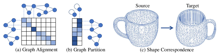
Figure 1: Graph learning tasks conducted in this paper.

To bridge the above theoretical-computational gap, we develop provably efficient iterative methods for the GW problem. Specifically, we propose two theoretically solid algorithms tailored to different graph learning tasks. Our first algorithm is the Bregman Alternating Projected Gradient (BAPG), which is also the first provable single-loop algorithm in the GW literature. The computational stumbling block here is the Birkhoff polytope constraint (i.e., polytope of doubly stochastic matrices) for the coupling matrix, as the associated Bregman projection is either computationally expensive or practically sensitive to hyperparameters. To address this issue, we are inspired to decouple the Birkhoff polytope as simplex constraints for rows and columns separately, and then execute the projected gradient descent in an alternating fashion. By leveraging the closed-form Bregman projection of the simplex constraint, BAPG only involves the matrix-vector/matrix-matrix multiplications and element-wise matrix operations at each iteration. In short, the proposed single-loop algorithm (BAPG) enjoys a variety of convenient properties: GPU-friendly implementation, robustness concerning the step size (i.e., the only hyper-parameter), and low memory cost. Nonetheless, the iterates generated by BAPG do not necessarily satisfy the Birkhoff polytope constraint and can only reach a critical point of the original GW problem asymptotically. To complement BAPG and avoid such a drawback, we revisit BPG from a fresh perspective and introduce our second algorithm — hybrid Bregman Projected Gradient (hBPG). In particular, we apply eBPG to get a good initial point and then use BPG to get to a critical point. Taking advantage of both eBPG and BPG, the resulting hBPG achieves a great balance between accuracy and efficiency.

Next, we investigate the convergence behavior of the proposed BAPG and hBPG. A key fact here is that the GW problem is a symmetric nonconvex quadratic program with Birkhoff polytope constraints. By fully exploring this structure, it is interesting to note that the GW problem satisfies the Luo-Tseng error bound condition (Luo and Tseng, 1992), which plays a vital role in our analysis. We first quantify the approximation bound for the fixed-point set of BAPG explicitly and the subsequent convergence result follows. Moreover, we prove the local linear convergence result of BPG and hBPG under the established local error bound property.

As a result of the developed theoretical results and algorithm characteristics, we are able to provide novel insights to help users to select the most suitable algorithm. In fact, BAPG is the best fit for the graph alignment and partition tasks (see Fig. 1 (a) and (b) for details), which can sacrifice some feasibility to gain both matching accuracy (i.e., performance measure) and computational efficiency. By contrast, hBPG is more suitable for the shape matching task (i.e., Fig. 1 (c)), where one of the quality metrics is the sharpness of the matching coupling. Hence, BAPG would be the sub-optimal choice due to its infeasibility issue. In terms of wall-clock time and modeling performance, extensive experiment results have shown that our methods consistently achieve superior performance on all graph learning tasks. It is also well worth noting that all theoretical insights have been well-supported by our experiment results. To sum up, this paper opens up an exciting avenue for realizing the benefits of GW in graph learning analysis.

2 Proposed Algorithms

In this section, we first formulate the GW distance as a nonconvex quadratic problem with Birkhoff polytope constraints. Then, we introduce two proposed algorithms — BAPG and hBPG, and further analyze their computational properties and applicable scenarios.

2.1 Problem Setup

The Gromov-Wasserstein (GW) distance was originally proposed in (Mémoli, 2011, 2014; Peyré et al., 2019) for quantifying the distance between two probability measures supported on heterogeneous metric spaces. More precisely:

Definition 2.1 (GW distance)

Suppose that we are given two unregistered compact metric spaces $(\mathcal{X},d_{X})$, $(\mathcal{Y},d_{Y})$ accompanied with Borel probability measures $\mu,\nu$ respectively. The GW distance between $\mu$ and $\nu$ is defined as

$$\inf_{\pi\in\Pi(\mu,\nu)}\iint|d_{X}(x,x^{\prime})-d_{Y}(y,y^{\prime})|^{2}d\pi(x,y)d\pi(x^{\prime},y^{\prime}),$$

where $\Pi(\mu,\nu)$ is the set of all probability measures on $\mathcal{X}\times\mathcal{Y}$ with $\mu$ and $\nu$ as marginals.

Intuitively, the GW distance is trying to preserve the isometric structure between two probability measures under optimal derivation. If a map pairs $x\rightarrow y$ and $x^{\prime}\rightarrow y^{\prime}$, then the distance between $x$ and $x^{\prime}$ is supposed to be close to the distance between $y$ and $y^{\prime}$. In view of these nice properties, the GW distance acts as a powerful modeling tool in structural data analysis, especially in graph learning; see, e.g., (Vayer et al., 2019; Xu et al., 2019b, a; Solomon et al., 2016; Peyré et al., 2016) and the references therein.

To start with our algorithmic developments, we consider the discrete case for simplicity and practicality, where $\mu$ and $\nu$ are two empirical distributions, i.e., $\mu=\sum_{i=1}^{n}\mu_{i}\delta_{x_{i}}$ and $\nu=\sum_{j=1}^{m}\nu_{j}\delta_{y_{j}}$. Then, the GW-distance admits the following reformulation:

$$\min_{\pi\in\mathbb{R}^{n\times m}}-\text{Tr}(D_{X}\pi D_{Y}\pi^{T})$$ (1)

$$\quad\,\text{s.t.}\quad\pi\mathbf{1}_{m}=\mu,\,\pi^{T}\mathbf{1}_{n}=\nu,\,\pi\geq 0,$$

where $D_{X}$ and $D_{Y}$ are two symmetric distance matrices.

2.2 Bregman Alternating Projected Gradient (BAPG)

Next, we present the proposed Bregman alternating projected gradient (BAPG) method, which is the first provable single-loop algorithm tailored to the GW distance computation. It is easy to observe that Problem (1) is a nonconvex quadratic program with polytope constraints. Naturally, if we want to invoke (Bregman) projected gradient descent type algorithms to address (1), the key difficulty lies in the Birkhoff constraint with respect to the coupling matrix $\pi$. In fact, all existing theoretically sound algorithms rely on an inner iterative algorithm to tackle the regularized optimal transport problem at each iteration, such as Sinkhorn (Cuturi, 2013) or semi-smooth Newton method (Li et al., 2020). Arguably, one of the main drawbacks of the double-loop scheme is its computational burden, which is not GPU friendly. To circumvent this drawback, we are motivated to handle the row and columns constraints separately (i.e., $C_{1}=\{\pi\geq 0:\pi\mathbf{1}_{m}=\mu\}$ and $C_{2}=\{\pi\geq 0:\pi^{T}\mathbf{1}_{n}=\nu\}$). The crux of BPAG is to take the alternating projected gradient descent step between $C_{1}$ and $C_{2}$. Moreover, by fully detecting the hidden structures, we are able to further benefit from the fact that the Bregman projection with respect to the negative entropy for the simplex constraint (e.g., $C_{1}$ and $C_{2}$) can be extremely efficient computed (Krichene et al., 2015). The above considerations lead to the closed-form updates in each iteration of BAPG:

where $\rho$ is the step size and $\odot$ denotes element-wise (Hadamard) matrix multiplication. BAPG enjoys several nice properties that are extremely attractive for medium or large-scale graph learning tasks. First, BAPG is a single-loop algorithm that only involves matrix-vector/matrix-matrix multiplications and element-wise matrix operations. All these operations are GPU-friendly. Second, different from the entropic regularization parameter in eBPG, BAPG is more robust to the step size $\rho$ in terms of solution performance. Third, BAPG only involves one memory operation of a large matrix with size $nm$. Notably, even for large-scale optimal transport problems, the main bottleneck is not floating-point computations, but rather time-consuming memory operations (Mai et al., 2021).

Theoretical Insights for BAPG

Now, we start to give the theoretical intuition of why BAPG will work well in practice. For simplicity, we consider the compact form for illustration:

$$\min_{\pi}f(\pi)+g_{1}(\pi)+g_{2}(\pi).$$ (3)

Here, $f(\pi)=-\text{Tr}(D_{X}\pi D_{Y}\pi^{T})$ is a nonconvex quadratic function; $g_{1}(\pi)=\mathbb{I}_{\{\pi\in C_{1}\}}$ and $g_{2}(\pi)=\mathbb{I}_{\{\pi\in C_{2}\}}$ are two indicator functions over closed convex polyhedral sets. To better understand the alternating projected scheme developed in (2), we adopt the operator splitting strategy to reformulate (3) as

$$\min_{\pi=w}\,f(\pi,w)+g_{1}(\pi)+g_{2}(w)$$ (4)

where $f(\pi,w)=-\text{Tr}(D_{X}\pi D_{Y}w^{T})$. Then, the BAPG update (2) can be interpreted as processing the alternating minimization scheme on the constructed penalized function, i.e.,

$$F_{\rho}(\pi,w)=f(\pi,w)+g_{1}(\pi)+g_{2}(w)+\rho D_{h}(\pi,w).$$

Here, $D_{h}(\cdot,\cdot)$ is the so-called Bregman divergence, i.e., $D_{h}(x,y):=h(x)-h(y)-\langle\nabla h(y),x-y\rangle,$ where $h(\cdot)$ is the Legendre function, e.g., $\tfrac{1}{2}\|x\|^{2}$, relative entropy $x\log x$, etc. For the $k$-th iteration, the BAPG update takes the form

$$\pi^{k+1} =\mathop{\arg\min}_{\pi\in C_{1}}\left\{f(\pi,w^{k})+\rho D_{h}(\pi,w^{k})\right\},$$ (5)

$$w^{k+1} =\mathop{\arg\min}_{w\in C_{2}}\left\{f(\pi^{k+1},w)+\rho D_{h}(w,\pi^{k+1})\right\}.$$

When $h$ is the relative entropy and we use the same variable to update $\pi$ and $w$, (2) can be derived from (5).

It is worth noting that the way to invoke the operator splitting strategy is not for the algorithm design as usual but instead to provide an intuitive way to explain why BAPG will work. As we shall see later, it plays an important role in deriving the approximation bound of the fix-point set of BAPG instead. Moreover, similar to the quadratic penalty method (Nocedal and Wright, 2006), BAPG is an infeasible method that can only converge to a critical point of (1) in an asymptotic sense. In other words, if we choose the parameter $\rho$ as a constant, there is always an infeasibility gap. Fortunately, BAPG is already able to achieve the desired performance for some graph learning tasks, especially those that care more about implementation efficiency and matching accuracy. Recently, (Vincent-Cuaz et al., 2021a) has proposed a relaxed version of GW distance for the graph partition task, which further corroborates our investigation that it is acceptable and promising to sacrifice some feasibility to gain other benefits. Moreover, Séjourné et al. (2021) has also proposed a closely related marginal relaxation. That is, we make $\pi=w$ and $F_{\rho}(\pi,\pi)$ is the objective introduced in (Séjourné et al., 2021). Unfortunately, they did not develop any provable algorithms for the unbalanced GW distance. In Sections 4.2 and 4.3, extensive experiments have been conducted to demonstrate that BAPG has superior performance compared with other existing baselines on graph alignment and partition tasks.

2.3 Hybrid Bregman Projected Gradient (hBPG)

To remedy the infeasible issue of BAPG, we revisit the Bregman proximal gradient descent (BPG) method, which is a feasible method for addressing the original problem (1) exactly. Such an approach has already been well-explored in some early works (Xu et al., 2019b). For the $k$-th iteration, BPG takes the form

$$\pi^{k+1}=\mathop{\arg\min}_{\pi\in C_{1}\cap C_{2}}\left\{\nabla f(\pi^{k})^{T}\pi+\frac{1}{t_{k}}D_{h}(\pi,\pi^{k})\right\},$$ (6)

where $t_{k}$ is the chosen step size. The core difficulty here is the need for an inner solver to tackle (6) efficiently. As it turns out, without the entropic regularizer, BPG suffers from the numerical instability issue. It is difficult for the inner solver to achieve the desired accuracy so as to guarantee convergence. Although Xu et al. (2019b) has provided a subsequential convergence result for BPG, it is too weak to guide the user in which scenarios BPG will potentially enjoy notable advantages. Such a state of affairs greatly limits its applicability. As we shall see later in Section 3.3, we explicitly analyze this stability issue and explain the reason rigorously. Different from graph alignment and partition tasks studied in Xu et al. (2019b, a), BPG-type methods are more attractive for applications that require a sharp matching map (such as shape correspondence), since the approximation (infeasibility) gap will dramatically affect the modeling performance.

We further exploit its local linear convergence property. Such a property guides us to take full advantage of both methods — BPG and eBPG. A natural idea is to apply eBPG to get a good initial point and then use BPG to reach critical points. It is reasonable to infer that the resulting hybrid method (denoted by hBPG) will achieve a trade-off between accuracy and efficiency. Comprehensive experiments conducted in Section 4.4 corroborate our theoretical insights.

At last, we summarize all the aforementioned algorithms in Table 1, aiming to provide a theoretically-supported guideline for readers on how to select the best-fit method based on their task properties.

Table 1: Comparison of various algorithms. “Exactly solve” means that algorithms can reach a critical point of the original GW problem instead of the approximation problem.

	Single-loop?	Provable?	Exactly solve (1)?
eBPG (Solomon et al., 2016)	No	Yes	No
BPG (Xu et al., 2019b)	No	Yes	Yes
BPG-S (Xu et al., 2019a)	Yes	No	No
FW (Titouan et al., 2019)	No	Yes	Yes
BAPG (our method)	Yes	Yes	No

3 Theoretical Results

In this section, we present all theoretical results conducted in this paper, including the approximation bound of the fix-point set of BAPG and its convergence analysis. At the heart of our analysis is that the following regularity condition holds for the GW problem (1).

Proposition 3.1 (Luo-Tseng Error Bound Condition for (1))

There exist scalars $\epsilon>0$ and $\tau>0$ such that

$$\operatorname{dist}2(\pi,\mathcal{X})\leq\tau\left\|\pi-\operatorname{proj}_{C_{1}\cap C_{2}}(\pi+D_{X}\pi D_{Y})\right\|,$$ (7)

whenever $\|\pi-\operatorname{proj}_{C_{1}\cap C_{2}}(\pi+D_{X}\pi D_{Y})\|\leq\epsilon$, where $\mathcal{X}$ is the critical point set of (3) defined by

$$\mathcal{X}=\{\pi\in C_{1}\cap C_{2}:0\in\nabla f(\pi)+\mathcal{N}_{C_{1}}(\pi)+\mathcal{N}_{C_{2}}(\pi)\}$$ (8)

and $\mathcal{N}_{C}(\pi)$ is the normal cone to $C$ at $\pi$.

Proof  $D_{X}$ and $D_{Y}$ are two symmetric matrices and $C_{1}\cap C_{2}$ is a convex polyhedral set. By invoking Theorem 2.3 in (Luo and Tseng, 1992), the Luo-Tseng local error bound condition (7) just holds for the feasible set $C_{1}\cap C_{2}$. That is,

$$\operatorname{dist}2(\pi,\mathcal{X})\leq\tau\left\|\pi-\operatorname{proj}_{C_{1}\cap C_{2}}(\pi+D_{X}\pi D_{Y})\right\|,$$ (9)

where $\pi\in C_{1}\cap C_{2}$. Then, we aim at extending (9) to the whole space. Define $\tilde{\pi}=\operatorname{proj}_{C_{1}\cap C_{2}}(\pi)$, we have

$$\operatorname{dist}2(\pi,\mathcal{X})\leq\|\pi-\tilde{\pi}\|+d(\tilde{\pi},\mathcal{X})\leq\|\pi-\tilde{\pi}\|+\tau\|\tilde{\pi}-\operatorname{proj}_{C_{1}\cap C_{2}}(\tilde{\pi}+D_{X}\tilde{\pi}D_{Y})\|$$ (10)

where the first inequality holds because of the triangle inequality, and the second one holds because of the fact $\tilde{\pi}\in C_{1}\cap C_{2}$ and (9). Apply the triangle inequality again, we have

$$\|\tilde{\pi}-\operatorname{proj}_{C_{1}\cap C_{2}}(\tilde{\pi}+D_{X}\tilde{\pi}D_{Y})\|$$ (11)

$$\leq \|\tilde{\pi}-\operatorname{proj}_{C_{1}\cap C_{2}}(\pi+D_{X}\pi D_{Y})\|+\|\operatorname{proj}_{C_{1}\cap C_{2}}(\pi+D_{X}\pi D_{Y})-\operatorname{proj}_{C_{1}\cap C_{2}}(\tilde{\pi}+D_{X}\tilde{\pi}D_{Y})\|$$

Since $\tilde{\pi}=\operatorname{proj}_{C_{1}\cap C_{2}}(\pi)$, owing to the fact that the projection operator onto a convex set $\operatorname{proj}_{C_{1}\cap C_{2}}(\cdot)$ is non-expensive, i.e., $\|\operatorname{proj}_{C_{1}\cap C_{2}}(x)-\operatorname{proj}_{C_{1}\cap C_{2}}(y)\|\leq\|x-y\|$ holds for any $x$ and $y$, we have

$$\|\tilde{\pi}-\operatorname{proj}_{C_{1}\cap C_{2}}(\pi+D_{X}\pi D_{Y})\| =\|\operatorname{proj}_{C_{1}\cap C_{2}}(\pi)-\operatorname{proj}_{C_{1}\cap C_{2}}(\operatorname{proj}_{C_{1}\cap C_{2}}(\pi+D_{X}\pi D_{Y}))\|$$ (12)

$$\leq\|\pi-\operatorname{proj}_{C_{1}\cap C_{2}}(\pi+D_{X}\pi D_{Y})\|,$$

and

$$\|\operatorname{proj}_{C_{1}\cap C_{2}}(\pi+D_{X}\pi D_{Y})-\operatorname{proj}_{C_{1}\cap C_{2}}(\tilde{\pi}+D_{X}\tilde{\pi}D_{Y})\| \leq\|(\pi+D_{X}\pi D_{Y})-(\tilde{\pi}+D_{X}\tilde{\pi}D_{Y})\|$$ (13)

$$\leq(\sigma_{\text{max}}(D_{X})\sigma_{\text{max}}(D_{Y})+1)\|\pi-\tilde{\pi}\|$$

where $\sigma_{\text{max}}(D_{X})$ and $\sigma_{\text{max}}(D_{Y})$ denote the maximum singular value of $D_{X}$ and $D_{Y}$, respectively. By substituting (11) and (13) into (10), we get

$$\operatorname{dist}2(\pi,\mathcal{X}) \leq(\tau\sigma_{\text{max}}(D_{X})\sigma_{\text{max}}(D_{Y})+\tau+1)\|\pi-\tilde{\pi}\|+\tau\|\pi-\operatorname{proj}_{C_{1}\cap C_{2}}(\pi+D_{X}\pi D_{Y})\|$$ (14)

$$\leq(\tau\sigma_{\text{max}}(D_{X})\sigma_{\text{max}}(D_{Y})+2\tau+1)\|\pi-\operatorname{proj}_{C_{1}\cap C_{2}}(\pi+D_{X}\pi D_{Y})\|$$

where the last inequality holds because of the fact that

$$\|\pi-\tilde{\pi}\|=\|\pi-\operatorname{proj}_{C_{1}\cap C_{2}}(\pi)\|=\min_{x\in C_{1}\cap C_{2}}\|\pi-x\|\leq\|\pi-\operatorname{proj}_{C_{1}\cap C_{2}}(\pi+D_{X}\pi D_{Y})\|.$$

By letting $\tau=\tau\sigma_{\text{max}}(D_{X})\sigma_{\text{max}}(D_{Y})+2\tau+1$, we get the desired result.  
As the GW problem is a nonconvex quadratic program with polytope constraint, we can invoke Theorem 2.3 in (Luo and Tseng, 1992) to conclude that the error bound condition (7) holds on the whole feasible set $C_{1}\cap C_{2}$. Proposition 3.1 extends (7) to the whole space $\mathbb{R}^{n\times m}$. This regularity condition is trying to bound the distance of any coupling matrix to the critical point set of the GW problem by its optimality residual, which is characterized by the difference for one step projected gradient descent. It turns out that this error bound condition plays an important role in quantifying the approximation bound for the fixed points set of BAPG explicitly.

3.1 Approximation Bound for the Fix-Point Set of BAPG

To start, we present one key lemma that shall be used in studying the approximation bound of BAPG.

Lemma 3.2

Let $C_{1}$ and $C_{2}$ be convex polyhedral sets. There exists a constant $M>0$ such that

$$\left\|\operatorname{proj}_{C_{1}}(x)+\operatorname{proj}_{C_{2}}(y)-2\operatorname{proj}_{C_{1}\cap C_{2}}\left(\frac{x+y}{2}\right)\right\|\leqslant M\left\|\operatorname{proj}_{C_{1}}(x)-\operatorname{proj}_{C_{2}}(y)\right\|,\forall x\in C_{1},y\in C_{2}.$$ (15)

Proof  we first convert the left-hand side of (15) to

$$\left\|\operatorname{proj}_{C_{1}}(x)-\operatorname{proj}_{C_{1}\cap C_{2}}\left(\frac{x+y}{2}\right)+\operatorname{proj}_{C_{2}}(y)-\operatorname{proj}_{C_{1}\cap C_{2}}\left(\frac{x+y}{2}\right)\right\|$$

$$\leq\ \sqrt{2}\left\|\left(\operatorname{proj}_{C_{1}\cap C_{2}}\left(\frac{x+y}{2}\right),\operatorname{proj}_{C_{1}\cap C_{2}}\left(\frac{x+y}{2}\right)\right)-(\operatorname{proj}_{C_{1}}(x),\operatorname{proj}_{C_{2}}(y))\right\|.$$

The core proof idea follows essentially from the observation that the inequality can be regarded as the stability of the optimal solution for a linear-quadratic problem, i.e.,

$$(p(r),q(r))=\begin{aligned} &\mathop{\arg\min}_{p,q}\frac{1}{2}\|x-p\|^{2}+\frac{1}{2}\|y-q\|^{2}\\ &\,\,\quad\text{s.t.}\,\,\quad p-q=r,\\ &\quad\quad\quad\quad p\in C_{1},q\in C_{2}.\end{aligned}$$ (16)

When $r=0$, the pair $(p(0),q(0))$ satisfies $p(0)=q(0)=\operatorname{proj}_{C_{1}\cap C_{2}}\left(\frac{x+y}{2}\right)$. Moreover, the parameter $r$ itself can be viewed as the perturbation quantity, which is indeed the right-hand side of (15). By invoking Theorem 4.1 in (Zhang and Luo, 2022), we can bound the distance between two optimal solutions by the perturbation quantity $r$, i.e.,

$$\|(p(0),q(0))-(p(r),q(r))\|\leq M\|r\|.$$

Remark 3.3

For any vector $r$, let $(p(r),q(r))$ be the optimal solution to (16). On the one hand, choosing $r=0$, it is easy to see that $p(0)=q(0)=\operatorname{proj}_{C_{1}\cap C_{2}}(\frac{x+y}{2})$. On the other hand, by choosing $r=\operatorname{proj}_{C_{1}}(x)-\operatorname{proj}_{C_{2}}(y)$, it is easy to see that $(p(r),q(r))=(\operatorname{proj}_{C_{1}}(x),\operatorname{proj}_{C_{2}}(y))$. Since Theorem 4.1 in (Zhang and Luo, 2022) implies that for any $r$, we have

$$\|(p(0),q(0))-(p(r),q(r))\|_{2}\leq M\|r\|_{2}$$

where $M$ only depends on $C_{1}$ and $C_{2}$. By choosing $r=\operatorname{proj}_{C_{1}}(x)-\operatorname{proj}_{C_{2}}(y)$, we have

$$\|(\operatorname{proj}_{C_{1}\cap C_{2}}(\frac{x+y}{2}),\operatorname{proj}_{C_{1}\cap C_{2}}(\frac{x+y}{2}))-(\operatorname{proj}_{C_{1}}(x),\operatorname{proj}_{C_{2}}(y))\leq M\|\operatorname{proj}_{C_{1}}(x)-\operatorname{proj}_{C_{2}}(y)\|_{2}.$$

 
Equipped with Lemma 3.2 and Proposition 3.1, it is not hard to obtain the following approximation result.

Proposition 3.4 (Approximation Bound of the Fix-point Set of BAPG)

The point
$(\pi^{\star},w^{\star})$ belongs to the fixed-point set $\mathcal{X}_{\text{BAPG}}$ of BAPG if it satisfies

$$\nabla f(w^{\star})+\rho(\nabla h(\pi^{\star})-\nabla h(w^{\star}))+p=0,$$ (17)

$$\nabla f(\pi^{\star})+\rho(\nabla h(w^{\star})-\nabla h(\pi^{\star}))+q=0,$$

where $p\in\mathcal{N}_{C_{1}}(\pi^{\star})$ and $q\in\mathcal{N}_{C_{2}}(w^{\star})$. Then, the infeasibility error satisfies $\|\pi^{\star}-w^{\star}\|\leq\frac{\tau_{1}}{\rho}$ and the gap between $\mathcal{X}_{\text{BAPG}}$ and $\mathcal{X}$ satisfies

$$\operatorname{dist}2\left(\frac{\pi^{\star}+w^{\star}}{2},\mathcal{X}\right)\leq\frac{\tau_{2}}{\rho},$$

where $\tau_{1}$ and $\tau_{2}$ are two constants.

Proof  Define $\hat{\pi}=\operatorname{proj}_{C_{1}\cap C_{2}}(\pi^{\star})$, we first want to argue the following inequality holds,

$$\|\hat{\pi}-\pi^{\star}\|+\|\hat{\pi}-w^{\star}\|\leq(2\kappa+1)\|\pi^{\star}-w^{\star}\|.$$

As the bounded linear regularity condition is satisfied for the polyhedral constraint, we have

$$\|\hat{\pi}-\pi^{\star}\|+\|\hat{\pi}-w^{\star}\| \leq 2\|\hat{\pi}-\pi^{\star}\|+\|\pi^{\star}-w^{\star}\|$$ (18)

$$=2\operatorname{dist}2(\pi^{\star},C_{1}\cap C_{2})+\|\pi^{\star}-w^{\star}\|$$

$$\leq(2\kappa+1)\|\pi^{\star}-w^{\star}\|.$$

Based on the stationary points defined in (17), we have,

$$\nabla f(w^{\star})^{T}(\hat{\pi}-\pi^{\star})+\rho(\nabla h(\pi^{\star})-\nabla h(w^{\star}))^{T}(\hat{\pi}-\pi^{\star})+p^{T}(\hat{\pi}-\pi^{\star})=0,p\in\mathcal{N}_{C_{1}}(\pi^{\star}),$$

$$\nabla f(\pi^{\star})^{T}(\hat{\pi}-w^{\star})+\rho(\nabla h(w^{\star})-\nabla h(\pi^{\star}))^{T}(\hat{\pi}-w^{\star})+q^{T}(\hat{\pi}-w^{\star})=0,q\in\mathcal{N}_{C_{2}}(w^{\star}).$$

Summing up the above two equations,

$$\nabla f(w^{\star})^{T}(\hat{\pi}-\pi^{\star})+\nabla f(\pi^{\star})^{T}(\hat{\pi}-w^{\star})+\rho(\nabla h(\pi^{\star})-\nabla h(w^{\star}))^{T}(w^{\star}-\pi^{\star})+p^{T}(\hat{\pi}-\pi^{\star})+q^{T}(\hat{\pi}-w^{\star})=0$$

$$\stackrel{{\scriptstyle(\clubsuit)}}{{\Rightarrow}} \nabla f(w^{\star})^{T}(\hat{\pi}-\pi^{\star})+\nabla f(\pi^{\star})^{T}(\hat{\pi}-w^{\star})-\rho(D_{h}(\pi^{\star},w^{\star})+D_{h}(w^{\star},\pi^{\star}))+p^{T}(\hat{\pi}-\pi^{\star})+q^{T}(\hat{\pi}-w^{\star})=0$$

$$\stackrel{{\scriptstyle(\spadesuit)}}{{\Rightarrow}} \nabla f(w^{\star})^{T}(\hat{\pi}-\pi^{\star})+\nabla f(\pi^{\star})^{T}(\hat{\pi}-w^{\star})-\rho(D_{h}(\pi^{\star},w^{\star})+D_{h}(w^{\star},\pi^{\star}))\geq 0,$$

where $(\clubsuit)$ holds as $(\nabla h(x)-\nabla h(y))^{T}(x-y)=D_{h}(x,y)+D_{h}(y,x)$ and $(\spadesuit)$ follows from the property of the normal cone. For instance, since $q\in\mathcal{N}_{C_{1}}(\pi^{\star})$, we have $q^{T}(\hat{\pi}-\pi^{\star})\leq 0$ (i.e., $\hat{\pi}\in C_{1}$). Therefore,

$$\rho(D_{h}(\pi^{\star},w^{\star})+D_{h}(w^{\star},\pi^{\star})) \leq\nabla f(w^{\star})^{T}(\hat{\pi}-\pi^{\star})+\nabla f(\pi^{\star})^{T}(\hat{\pi}-w^{\star})$$

$$\leq\|\nabla f(w^{\star})\|\|\hat{\pi}-\pi^{\star}\|+\|\nabla f(\pi^{\star})\|\|\hat{\pi}-w^{\star}\|$$

$$\leq L_{f}(\|\hat{\pi}-\pi^{\star}\|+\|\|\hat{\pi}-w^{\star}\|)$$

$$\stackrel{{\scriptstyle\eqref{eq:blr_inf}}}{{\leq}}(2\kappa+1)L_{f}\|\pi^{\star}-w^{\star}\|.$$

The next to last inequality holds as $f(\cdot)$ is a quadratic function and the effective domain $C_{1}\cap C_{2}$ is bounded. Thus, the norm of its gradient will naturally have a constant upper bound, i.e., $L_{f}=\sigma_{\text{max}}(D_{X})\sigma_{\text{max}}(D_{Y})$. As $h$ is a $\sigma$-strongly convex, we have

$$D_{h}(\pi^{\star},w^{\star})\geq\frac{\sigma}{2}\|\pi^{\star}-w^{\star}\|^{2}.$$

Together with this property, we can quantify the infeasibility error $\|\pi^{\star}-w^{\star}\|$,

$$\|\pi^{\star}-w^{\star}\|\leq\frac{(2\kappa+1)L_{f}}{\delta\rho}.$$ (19)

When $\rho\rightarrow+\infty$, it is easy to observe that the infeasibility error term $\|\pi^{\star}-w^{\star}\|$ will shrink to zero. More importantly, if $\pi^{\star}=w^{\star}$, then $X_{\text{BAPG}}$ will be identical to $\mathcal{X}$. Next, we target at quantifying the approximation gap between the fixed-point set of BAPG and the critical point set of the original problem (1). Upon (17), we have

$$\nabla f\left(\frac{\pi^{\star}+w^{\star}}{2}\right)+\frac{p+q}{2}=0,$$

where $\nabla f(\cdot)$ is a linear operator. By applying the Luo-Tseng local error bound condition of (1), i.e., Proposition 3.1, we have

$$\operatorname{dist}2\left(\frac{\pi^{\star}+w^{\star}}{2},\mathcal{X}\right) \leq\tau\left\|\frac{\pi^{\star}+w^{\star}}{2}-\operatorname{proj}_{C_{1}\cap C_{2}}\left(\frac{\pi^{\star}+w^{\star}}{2}-\nabla f\left(\frac{\pi^{\star}+w^{\star}}{2}\right)\right)\right\|$$

$$=\tau\left\|\frac{\pi^{\star}+w^{\star}}{2}-\operatorname{proj}_{C_{1}\cap C_{2}}\left(\frac{\pi^{\star}+p+w^{\star}+q}{2}\right)\right\|$$

$$\stackrel{{\scriptstyle(\clubsuit)}}{{=}}\frac{\tau}{2}\left\|\operatorname{proj}_{C_{1}}(\pi^{\star}+p)+\operatorname{proj}_{C_{1}}(w^{\star}+q)-2\operatorname{proj}_{C_{1}\cap C_{2}}\left(\frac{\pi^{\star}+p+w^{\star}+q}{2}\right)\right\|$$

$$\stackrel{{\scriptstyle(\spadesuit)}}{{\leq}}\frac{M\tau}{2}\|\pi^{\star}-w^{\star}\|,$$

where $(\clubsuit)$ holds due to the normal cone property, that is, $\operatorname{proj}_{C}(x+z)=x$ for any $x\in C$ and $z\in\mathcal{N}_{C}(x)$, and $(\spadesuit)$ follows from Lemma 3.2. Incorporating with (19), the approximation bound for BAPG has been characterized quantitatively, i.e.,

$$\operatorname{dist}2\left(\frac{\pi^{\star}+w^{\star}}{2},\mathcal{X}\right)\leq\frac{(2\kappa+1)L_{f}M}{2\delta\rho}.$$

 

Remark 3.5

If $\pi^{\star}=w^{\star}$, then $\mathcal{X}_{\text{BAPG}}$ is identical to $\mathcal{X}$ and BAPG can reach a critical point of the GW problem (1). Proposition 3.4 indicates that as $\rho\rightarrow+\infty$, the infeasibility error term $\|\pi^{\star}-w^{\star}\|$ shrinks to zero and thus BAPG converges to a critical point of (1) in an asymptotic way. Furthermore, it explicitly quantifies the approximation gap when we select the parameter $\rho$ as a constant. The explicit form of $\tau_{1}$ and $\tau_{2}$ only depend on the problem itself, including $\sigma_{\textnormal{max}}(D_{X})\sigma_{\textnormal{max}}(D_{Y})$, the constant for the Luo-Tseng error bound condition in Proposition 3.1 and so on.

3.2 Convergence Analysis of BAPG

A further natural question is whether BAPG will converge or not. We answer the question in the affirmative. Specifically, we show that under several canonical assumptions, any limit point of BAPG belongs to $\mathcal{X}_{\text{BAPG}}$. Towards that end, let us first establish the sufficient decrease property of BAPG based on the potential function $F_{\rho}(\cdot)$,

Proposition 3.6

Let $\{(\pi^{k},w^{k})\}_{k\geq 0}$ be the sequence generated by BAPG. Suppose that $D_{h}(\cdot,\cdot)$ is symmetric on the whole sequence. Then, we have

$$F_{\rho}(\pi^{k+1},w^{k+1})-F_{\rho}(\pi^{k},w^{k})\leq-\rho D_{h}(\pi^{k},\pi^{k+1})-\rho D_{h}(w^{k},w^{k+1}).$$ (20)

Proof  We first observe from the optimality conditions of main updates, i.e.,

$$0\in\nabla_{\pi}f(\pi^{k},w^{k})+\rho(\nabla h(\pi^{k+1})-\nabla h(w^{k}))+\partial g_{1}(\pi^{k+1})$$ (21)

$$0\in\nabla_{w}f(\pi^{k+1},w^{k})+\rho(\nabla h(w^{k+1})-\nabla h(\pi^{k+1}))+\partial g_{2}(w^{k+1})$$ (22)

where $g_{1}(\pi)=I_{\{\pi\in C_{1}\}}$ and $g_{2}(w)=I_{\{w\in C_{2}\}}$. Due to the convexity of $g_{1}(\cdot)$, it is natural to obtain,

$$g_{1}(\pi^{k})-g_{1}(\pi^{k+1}) \geq-\langle\nabla_{\pi}f(\pi^{k},w^{k})+\rho(\nabla h(\pi^{k+1})-\nabla h(w^{k})),\pi^{k}-\pi^{k+1}\rangle$$

$$=-\langle\nabla_{\pi}f(\pi^{k},w^{k}),\pi^{k}-\pi^{k+1}\rangle+\langle\rho(\nabla h(\pi^{k+1})-\nabla h(w^{k})),\pi^{k+1}-\pi^{k}\rangle$$

As $f(\pi,w)=-\text{tr}(D_{X}\pi D_{Y}w^{T})$ is a bilinear function, we have,

$$f(\pi^{k},w^{k})-f(\pi^{k+1},w^{k})-\langle\nabla_{\pi}f(\pi^{k},w^{k}),\pi^{k}-\pi^{k+1}\rangle=0.$$

Consequently, we get

$$f(\pi^{k},w^{k})+g_{1}(\pi^{k})-f(\pi^{k+1},w^{k})-g_{1}(\pi^{k+1})\geq\rho\langle\nabla h(\pi^{k+1})-\nabla h(w^{k}),\pi^{k+1}-\pi^{k}\rangle.$$ (23)

Similarly, based on the $w$-update, we obtain

$$f(\pi^{k+1},w^{k})+g_{2}(w^{k})-f(\pi^{k+1},w^{k+1})-g_{2}(w^{k+1})\geq\rho\langle\nabla h(w^{k+1})-\nabla h(\pi^{k+1}),w^{k+1}-w^{k}\rangle.$$ (24)

Combine with (23) and (24), we obtain

$$f(\pi^{k},w^{k})+g_{1}(\pi^{k})+g_{2}(w^{k})-f(\pi^{k+1},w^{k+1})-g_{1}(\pi^{k+1})-g_{2}(w^{k+1})$$ (25)

$$\geq \rho\langle\nabla h(\pi^{k+1})-\nabla h(w^{k}),\pi^{k+1}-\pi^{k}\rangle+\rho\langle\nabla h(w^{k+1})-\nabla h(\pi^{k+1}),w^{k+1}-w^{k}\rangle.$$

The right-hand side can be further simplified,

$$\rho\langle\nabla h(\pi^{k+1})-\nabla h(w^{k}),\pi^{k+1}-\pi^{k}\rangle+\rho\langle\nabla h(w^{k+1})-\nabla h(\pi^{k+1}),w^{k+1}-w^{k}\rangle$$

$$\stackrel{{\scriptstyle(\clubsuit)}}{{=}} \rho(D_{h}(\pi^{k},\pi^{k+1})+D_{h}(\pi^{k+1},w^{k})-D_{h}(\pi^{k},w^{k}))+\rho(D_{h}(w^{k},w^{k+1})+$$

$$D_{h}(w^{k+1},\pi^{k+1})-D_{h}(w^{k},\pi^{k+1}))$$

$$\stackrel{{\scriptstyle(\spadesuit)}}{{=}} \rho D_{h}(\pi^{k},\pi^{k+1})+\rho D_{h}(w^{k},w^{k+1})-\rho D_{h}(\pi^{k},w^{k})+\rho D_{h}(\pi^{k+1},w^{k+1}).$$

Here, $(\clubsuit)$ uses the fact that the three-point property of Bregman divergence holds, i.e., For any $y,z\in$ int $\operatorname{dom}h$ and $x\in\operatorname{dom}h$,

$$D_{h}(x,z)-D_{h}(x,y)-D_{h}(y,z)=\langle\nabla h(y)-\nabla h(z),x-y\rangle.$$

Moreover, $(\spadesuit)$ holds as $D_{h}(\cdot,\cdot)$ is symmetric on the whole sequence. To proceed, this together with (25) implies

$$F_{\rho}(\pi^{k+1},w^{k+1})-F_{\rho}(\pi^{k},w^{k})\leq-\rho D_{h}(\pi^{k},\pi^{k+1})-\rho D_{h}(w^{k},w^{k+1}).$$ (26)

Summing up (26) from $k=0$ to $+\infty$, we obtain

$$F_{\rho}(\pi^{\infty},w^{\infty})-F_{\rho}(\pi^{0},w^{0})\leq-\kappa_{1}\sum_{k=0}^{\infty}\left(D_{h}(\pi^{k},\pi^{k+1})+D_{h}(w^{k},w^{k+1})\right).$$

 
As the potential function $F_{\rho}(\cdot,\cdot)$ is coercive and $\{(\pi^{k},w^{k})\}_{k\geq 0}$ is a bounded sequence, it means the left-hand side is bounded, which implies

$$\sum_{k=0}^{\infty}\left(D_{h}(\pi^{k},\pi^{k+1})+D_{h}(w^{k},w^{k+1})\right)<+\infty.$$

Both $\{D_{h}(\pi^{k},\pi^{k+1})\}_{k\geq 0}$ and $\{D_{h}(w^{k},w^{k+1})\}_{k\geq 0}$ converge to zero. Thus, the following convergence result holds.

Theorem 3.7 (Subsequent Convergence of BAPG)

Any limit point of the sequence
$\{(\pi^{k},w^{k})\}_{k\geq 0}$ generated by BAPG belongs to $\mathcal{X}_{\text{BAPG}}$.

Proof  Let $(\pi^{\infty},w^{\infty})$ be a limit point of the sequence $\{(\pi^{k},w^{k})\}_{k\geq 0}$. Then, there exists a sequence $\{n_{k}\}_{k\geq 0}$ such that $\{(\pi^{n_{k}},w^{n_{k}})\}_{k\geq 0}$ converges to $(\pi^{\infty},w^{\infty})$. Replacing $k$ by $n_{k}$ in (21) and (22), taking limits on both sides as $k\rightarrow\infty$

$$0\in\nabla_{\pi}f(\pi^{\infty},w^{\infty})+\rho(\nabla h(\pi^{\infty})-\nabla h(w^{\infty}))+\partial g_{1}(\pi^{\infty})$$

$$0\in\nabla_{w}f(\pi^{\infty},w^{\infty})+\rho(\nabla h(w^{\infty})-\nabla h(\pi^{\infty}))+\partial g_{2}(w^{\infty}).$$

Based on the fact that $\nabla_{\pi}f(\pi^{\infty},w^{\infty})=\nabla f(w^{\infty})$ and $\nabla_{w}f(\pi^{\infty},w^{\infty})=\nabla f(\pi^{\infty})$, it can be easily concluded that $(\pi^{\infty},w^{\infty})\in\mathcal{X}_{\text{BAPG}}$.  

Remark 3.8

The symmetric assumption in Proposition 3.6 does not hold for the KL divergence in general. However, if we add a mild condition that the asymmetric ratio is bounded for iterations, similar results can be achieved. Moreover, when $h$ is a quadratic function, we can further obtain the global convergence result under the Kurdyka-Lojasiewicz analysis framework developed in (Attouch et al., 2010, 2013).

More importantly, the above subsequence convergence result can be extended to the global convergence if the Legendre function $h(\cdot)$ is quadratic.

Theorem 3.9 (Global Convergence of BAPG — Quadratic Case)

The sequence
$\{(\pi^{k},w^{k})\}_{k\geq 0}$ converges to a critical point of $F_{\rho}(\pi,w)$.

Proof  To invoke the Kurdyka-Lojasiewicz analysis framework developed in (Attouch et al., 2010, 2013), we have to establish two crucial properties — sufficient decrease and safeguard condition. The first one has already been proven in Proposition 3.6. Then, we would like to show that there exists a constant $\kappa_{2}$ such that,

$$\operatorname{dist}2(0,\partial F_{\rho}(\pi^{k+1},w^{k+1}))\leq\kappa_{2}(\|\pi^{k+1}-\pi^{k}\|+\|w^{k+1}-w^{k}\|).$$

At first, noting that

$$\partial F_{\rho}(\pi^{k+1},w^{k+1})=\left[\begin{aligned} &\nabla_{\pi}f(\pi^{k+1},w^{k+1})+\rho(\pi^{k+1}-w^{k+1})+\partial g_{1}(\pi^{k+1})\\ &\nabla_{w}f(\pi^{k+1},w^{k+1})+\rho(w^{k+1}-\pi^{k+1})+\partial g_{2}(w^{k+1})\end{aligned}\right].$$

Again, together with the updates (21) and (22), this implies

$$\operatorname{dist}2^{2}(\mathbf{0},\partial F_{\rho}(\pi^{k+1},w^{k+1})) \leq\|\nabla_{\pi}f(\pi^{k+1},w^{k+1})-\nabla_{\pi}f(\pi^{k},w^{k})\|^{2}+\rho\|w^{k}-w^{k+1}\|^{2}$$

$$+\|\nabla_{w}f(\pi^{k+1},w^{k})-\nabla_{w}f(\pi^{k+1},w^{k+1})\|^{2}$$

$$\leq(\sigma^{2}_{\text{max}}(D_{X})\sigma^{2}_{\text{max}}(D_{Y})+\rho)\|w^{k}-w^{k+1}\|^{2},$$

where $\sigma_{\text{max}}(\cdot)$ denotes the maximum singular value. By letting $\kappa_{2}=\sqrt{\sigma^{2}_{\text{max}}(D_{X})\sigma^{2}_{\text{max}}(D_{Y})+\rho}$, we get the desired result.  

To the best of our knowledge, the convergence analysis of alternating projected gradient descent methods has only been given under the convex setting, see (Wang and Bertsekas, 2016; Nedić, 2011) for details. In this paper, by heavily exploiting the error bound condition of the GW problem, we take the first step and provide a new path to conduct the analysis of alternating projected descent method for nonconvex problems, which could be of independent interest.

3.3 Local Linear Convergence of BPG and hBPG

Next, we investigate the convergence behavior of BPG when applied to problem (1). At the heart of our convergence rate analysis is the Luo-Tseng local error bound condition (cf. Proposition 3.1), which has been demonstrated as a crucial tool to establish the linear convergence rate of first-order algorithms (Zhou and So, 2017). Recall that a sequence $\{x^{k}\}_{k\geq 0}$ is said to converge R-linearly (resp. Q-linearly) to a point $x^{\infty}$ if there exist constants $\gamma>0$ and $\eta\in(0,1)$ such that $\|x^{k}-x^{\infty}\|\leq\gamma\eta^{k}$ for all $k\geq 0$ (resp. if there exists an index $K\geq 0$ and a constant $\eta\in(0,1)$ such that $\|x^{k+1}-x^{\infty}\|/\|x^{k}-x^{\infty}\|\leq\eta$ for all $k\geq K$).

Theorem 3.10 (Local Linear Convergence of BPG)

Suppose that in Problem (1), the step size $t_{k}$ in (6) satisfies $0<\underline{t}\leq t_{k}<\overline{t}\leq{\sigma}/{L_{f}}$ for $k\geq 0$ where $\underline{t},\overline{t}$ are given constants and $L_{f}$ is the gradient Lipschitz constant of $f$. Moreover, suppose that the sequence $\{\pi^{k}\}_{k\geq 0}$ has a element-wise lower bound, i.e., $\pi_{k}\geq\epsilon>0$, the sequence of solutions $\{\pi^{k}\}_{k\geq 0}$ generated by BPG converges R-linearly to an element in the critical point set $\mathcal{X}$.

In terms of the convergence analysis of first-order iterative methods solving (1), the Luo-Tseng Local Error Bound Condition (cf. Proposition 3.1) has been demonstrated as a crucial tool to unveiling the linear convergence rate under the convex setting (Zhou and So, 2017; Hou et al., 2013). The following folkloric result provides a unified template for the convergence rate analysis of first-order methods:

Fact 3.11

(cf. Fact 1 in Zhou and So (2017)) Consider the optimization problem (1), whose the critical point set $\mathcal{X}$ is assumed to be non-empty. Suppose that the generated sequence $\left\{\pi^{k}\right\}_{k\geq 0}$ satisfying the following properties:

1. (Sufficient Descent) There exist a constant $\kappa_{1}>0$ and an index $k_{1}\geq 0$ such that for $k\geq k_{1}$,

   $$F\left(\pi^{k+1}\right)-F\left(\pi^{k}\right)\leq-\kappa_{1}\left\|\pi^{k+1}-\pi^{k}\right\|^{2}.$$

2. (Cost-to-Go Estimate) There exist a constant $\kappa_{2}>0$ and an index $k_{2}\geq 0$ such that for $k\geq k_{2}$,

   $$F\left(\pi^{k+1}\right)-F(\pi^{\star})\leq\kappa_{2}\left(\operatorname{dist}2^{2}\left(\pi^{k},\mathcal{X}\right)+\left\|\pi^{k+1}-\pi^{k}\right\|^{2}\right),$$

   where $\pi^{\star}$ is the limit point of the sequence $\{\pi^{k}\}_{k\geq 0}$.

3. (Safeguard) There exist a constant $\kappa_{3}>0$ and an index $k_{3}\geq 0$ such that for $k\geq k_{3}$,

   $$\left\|R(\pi^{k})\right\|_{2}\leq\kappa_{3}\left\|\pi^{k+1}-\pi^{k}\right\|_{2},$$

   where $R(\pi^{k})$ is the proximal residual function, defined as

   $$R(\pi^{k})=\|\pi^{k}-\operatorname{prox}_{g}(\pi^{k}-\nabla f(\pi^{k}))\|.$$

Suppose further that Problem (1) possesses the Luo-Tseng error bound condition. Then, the sequence $\left\{F\left(\pi^{k}\right)\right\}_{k\geq 0}$ converges $Q$-linearly to $F(\pi^{\star})$ and the sequence $\left\{\pi^{k}\right\}_{k\geq 0}$ converges $R$-linearly to some $\pi^{\star}\in\mathcal{X}$.

Before giving the proof details, we would like to highlight the difference from the technique used in (Hou et al., 2013) and (Zhou and So, 2017). The vanilla analysis in (Hou et al., 2013) and (Zhou and So, 2017) can only handle the structured convex problem but GW is nonconvex. We have to exploit the isolation property around the local region to establish the cost-to-go estimate property. Intuitively, the isolation property means that the sequence $\{\pi^{k}\}_{k\geq 0}$ will eventually settle down at a Euclidean ball. More precisely, we refer the reader to Assumption 3.12 for details, which can be verified for the Gromov Wasserstein problem. The geometry from the Bregman divergence can be non-Euclidean. It is not an easy task to extend the analysis in Euclidean space to the general Bregman distance-derived metric space.

Assumption 3.12

For any $\bar{\pi}\in\mathcal{x}$, there exists $\delta>0$ so that $F(\pi)=F(\bar{\pi})$ whenever $\pi\in\mathcal{X}$ and $\|\pi-\bar{\pi}\|<\delta$.

Proof 

Step 1: Sufficient Decrease Property

It is worthwhile noting that $f(\pi)$ is a quadratic function, i.e., $f(\pi)=-\text{Tr}(D_{X}\pi D_{Y}\pi^{T})$, then $f(\pi)$ is gradient Lipschitz continuous with the modulu constant $\sigma_{\text{max}}(D_{X})\sigma_{\text{max}}(D_{Y})$, where $\sigma_{\text{max}}(\cdot)$ denotes the largest singular value. To simplify the notation, let $L_{f}=\sigma_{\text{max}}(D_{X})\sigma_{\text{max}}(D_{Y})$.

$$F(\pi^{k+1})-F(\pi^{k})$$

$$\leq f(\pi^{k})+\nabla f(\pi^{k})^{T}(\pi^{k+1}-\pi^{k})+\frac{L_{f}}{2}\|\pi^{k+1}-\pi^{k}\|^{2}+g(\pi^{k+1})-f(\pi^{k})-g(\pi^{k})$$

$$\stackrel{{\scriptstyle(\clubsuit)}}{{\leq}}\nabla f(\pi^{k})^{T}(\pi^{k+1}-\pi^{k})+\frac{L_{f}}{\sigma}D_{h}(\pi^{k+1},\pi^{k})+g(\pi^{k+1})-g(\pi^{k})$$

$$=\nabla f(\pi^{k})^{T}(\pi^{k+1}-\pi^{k})+\frac{1}{t_{k}}D_{h}(\pi^{k+1},\pi^{k})+g(\pi^{k+1})-g(\pi^{k})+\left(\frac{L_{f}}{\sigma}-\frac{1}{t_{k}}\right)D_{h}(\pi^{k+1},\pi^{k})$$

$$=\hat{F}(\pi^{k+1};\pi^{k})-\hat{F}(\pi^{k};\pi^{k})+\left(\frac{L_{f}}{\sigma}-\frac{1}{t_{k}}\right)D_{h}(\pi^{k+1},\pi^{k})$$

$$\stackrel{{\scriptstyle(\spadesuit)}}{{\leq}}\left(\frac{L_{f}}{\sigma}-\frac{1}{t_{k}}\right)D_{h}(\pi^{k+1},\pi^{k})$$

$$\stackrel{{\scriptstyle(\clubsuit)}}{{\leq}}-\left(\frac{1}{t_{k}}-\frac{L_{f}}{\sigma}\right)\|\pi^{k+1}-\pi^{k}\|^{2},$$

where $(\clubsuit)$ holds due to the fact $D_{h}(\pi^{k+1}-\pi^{k})\geq\frac{\sigma}{2}\|\pi^{k+1}-\pi^{k}\|^{2}$ and $(\spadesuit)$ follows as the optimal solution of $\hat{F}(\pi;\pi^{k})$ is $\pi^{k+1}$, i.e., (6). By letting $\kappa_{1}=\frac{1}{t_{k}}-\frac{L_{f}}{\sigma}>0$, we get the desired result.

Step 2: Cost-to-Go Estimate Property

Let $\overline{\pi}^{k}$ be the projection of $\pi^{k}$ onto $\mathcal{X}$. Again, we aim at exploiting the structure information from the BPG update, i.e., (6). Similarly, as the optimal solution of $\hat{F}(\pi;\pi^{k})$ is $\pi^{k+1}$, we have,

$$\hat{F}(\pi^{k+1};\pi^{k})\leq\hat{F}(\overline{\pi}^{k};\pi^{k})$$

$$\Rightarrow \nabla f(\pi^{k})^{T}\pi^{k+1}+\frac{1}{t_{k}}D_{h}(\pi^{k+1},\pi^{k})+g(\pi^{k+1})\leq\nabla f(\pi^{k})^{T}\overline{\pi}^{k}+\frac{1}{t_{k}}D_{h}(\overline{\pi}^{k},\pi^{k})+g(\overline{\pi}^{k})$$

$$\Rightarrow \nabla f(\pi^{k})^{T}(\pi^{k+1}-\overline{\pi}^{k})+g(\pi^{k+1})-g(\overline{\pi}^{k})\leq\frac{1}{t_{k}}D_{h}(\overline{\pi}^{k},\pi^{k})-\frac{1}{t_{k}}D_{h}(\pi^{k+1},\pi^{k}).$$

It implies

$$\nabla f(\pi^{k})^{T}(\pi^{k+1}-\overline{\pi}^{k})+g(\pi^{k+1})-g(\overline{\pi}^{k})\leq\frac{1}{t_{k}}D_{h}(\overline{\pi}^{k},\pi^{k})\leq\frac{L}{t_{k}}\|\overline{\pi}^{k}-\pi^{k}\|_{F}^{2}\leq\frac{L}{\underline{t}}\operatorname{dist}2^{2}(\pi^{k},\mathcal{X}),$$

where $L$ is a constant.

By the mean value theorem and $f$ is continuous differentiable, there exists a $\hat{\pi}^{k}\in[\overline{\pi}^{k},\pi^{k+1}]$ such that,

$$f(\pi^{k+1})-f(\overline{\pi}^{k})=\nabla f(\hat{\pi}^{k})^{T}(\pi^{k+1}-\overline{\pi}^{k}).$$

Hence, we compute,

$$F(\pi^{k+1})-F(\overline{\pi}^{k})$$

$$= \nabla f(\hat{\pi}^{k})^{T}(\pi^{k+1}-\overline{\pi}^{k})+g(\pi^{k+1})-g(\overline{\pi}^{k})$$

$$= \nabla f({\pi}^{k})^{T}(\pi^{k+1}-\overline{\pi}^{k})+g(\pi^{k+1})-g(\overline{\pi}^{k})+(\nabla f(\hat{\pi}^{k})-\nabla f({\pi}^{k}))^{T}(\pi^{k+1}-\overline{\pi}^{k})$$

$$\leq \frac{L}{\underline{t}}\operatorname{dist}2^{2}(\pi^{k},\mathcal{X})+(\nabla f(\hat{\pi}^{k})-\nabla f({\pi}^{k}))^{T}(\pi^{k+1}-\overline{\pi}^{k})$$

$$\leq \frac{L}{\underline{t}}\operatorname{dist}2^{2}(\pi^{k},\mathcal{X})+L_{f}\|\hat{\pi}^{k}-{\pi}^{k}\|\|\pi^{k+1}-\overline{\pi}^{k}\|$$

$$\leq \frac{L}{\underline{t}}\operatorname{dist}2^{2}(\pi^{k},\mathcal{X})+L_{f}\left(\|\hat{\pi}^{k}-{\pi}^{k+1}\|+\|{\pi}^{k+1}-\pi^{k}\|\right)\|\pi^{k+1}-\overline{\pi}^{k}\|$$

$$\leq \frac{L}{\underline{t}}\operatorname{dist}2^{2}(\pi^{k},\mathcal{X})+L_{f}\left(\|\overline{\pi}^{k}-{\pi}^{k+1}\|+\|{\pi}^{k+1}-\pi^{k}\|\right)\|\pi^{k+1}-\overline{\pi}^{k}\|$$

$$\leq \frac{L}{\underline{t}}\operatorname{dist}2^{2}(\pi^{k},\mathcal{X})+\frac{3L_{f}}{2}\|\overline{\pi}^{k}-{\pi}^{k+1}\|^{2}+\frac{L_{f}}{2}\|{\pi}^{k+1}-\pi^{k}\|^{2}$$

$$\leq \frac{L}{\underline{t}}\operatorname{dist}2^{2}(\pi^{k},\mathcal{X})+{3L_{f}}\|\overline{\pi}^{k}-{\pi}^{k}\|^{2}+\frac{7L_{f}}{2}\|{\pi}^{k+1}-\pi^{k}\|^{2}$$

$$= \left(\frac{L}{\underline{t}}+3L_{f}\right)\operatorname{dist}2^{2}(\pi^{k},\mathcal{X})+\frac{7L_{f}}{2}\|{\pi}^{k+1}-\pi^{k}\|^{2}$$

$$\leq \max\left(\left(\frac{L}{\underline{t}}+3L_{f}\right),\frac{7L_{f}}{2}\right)\left(\operatorname{dist}2^{2}(\pi^{k},\mathcal{X})+\|{\pi}^{k+1}-\pi^{k}\|^{2}\right).$$

For the relative entropy function $h(x)=x\log x$, we can show that $L=\frac{2}{\epsilon}=2L_{h}(K)$. Since the sequence $\{\pi^{k}\}_{k\geq 0}$ is lower bounded by the constant $\epsilon$, i.e., $\pi^{k}\geq\epsilon I$, then we can conclude

$$D_{h}(\overline{\pi}^{k},\pi^{k})\leq\frac{2}{\epsilon}\|\overline{\pi}^{k}-\pi^{k}\|_{F}^{2},$$

Let $I=\{(i,j)\mid\overline{\pi}^{k}_{ij}\geq\frac{\epsilon}{2}\}$ and $\bar{I}$ be its supplementary set. Then, we have

$$D_{h}(\overline{\pi}^{k},\pi^{k})= \sum_{(i,j)\in I}D_{h}(\overline{\pi}^{k}_{ij},\pi^{k}_{ij})+\sum_{(i,j)\in\bar{I}}D_{h}(\overline{\pi}^{k}_{ij},\pi^{k}_{ij})$$

$$\leq \sum_{(i,j)\in I}\frac{2}{\epsilon}(\overline{\pi}^{k}_{ij}-\pi^{k}_{ij})^{2}+\sum_{(i,j)\in\bar{I}}D_{h}(\overline{\pi}^{k}_{ij},\pi^{k}_{ij})$$

$$\leq \sum_{(i,j)\in I}\frac{2}{\epsilon}(\overline{\pi}^{k}_{ij}-\pi^{k}_{ij})^{2}+\sum_{(i,j)\in\bar{I}}(\pi^{k}_{ij}-\overline{\pi}^{k}_{ij})$$

$$\leq \sum_{(i,j)\in I}\frac{2}{\epsilon}(\overline{\pi}^{k}_{ij}-\pi^{k}_{ij})^{2}+\sum_{(i,j)\in\bar{I}}\frac{2}{\epsilon}(\pi^{k}_{ij}-\overline{\pi}^{k}_{ij})^{2}$$

$$= \frac{2}{\epsilon}\|\overline{\pi}-\pi\|_{F}^{2},$$

where the first inequality holds because the second-order direvative $h^{\prime\prime}(x)=\frac{1}{x}\leq\frac{2}{\epsilon}$ for all $x\geq\frac{\epsilon}{2}$, the second inequality holds because $D_{h}(x,y)=x\log\frac{x}{y}+y-x\leq y-x$ if $x\leq y$, and the third inequality holds because $\pi^{k}_{ij}-\overline{\pi}^{k}_{ij}\geq\epsilon-\frac{\epsilon}{2}=\frac{\epsilon}{2}$ for all $(i,j)\in\bar{I}$.

At last, by applying Lemma 3.1 in (Luo and Tseng, 1992), we know $F(\cdot)$ enjoys the isolation property around the local region. Therefore, by letting $\kappa_{2}=\max\left(\left(\frac{2L_{h}(K)}{\underline{t}}+3L_{f}\right),\frac{7L_{f}}{2}\right)$, we obtain the desired result.

Step 3: Safeguard Property

Again, invoking the optimality condition of the main BPG update (6), we have

$$0\in\nabla f(\pi^{k})+\partial g(\pi^{k+1})+\frac{1}{t_{k}}\nabla D_{h}(\pi^{k+1},\pi^{k})$$ (27)

$$0\in\nabla f(\pi^{k+1})+\partial g(\pi^{k+1})+\nabla f(\pi^{k})-\nabla f(\pi^{k+1})+\frac{1}{t_{k}}(\nabla h(\pi^{k+1})-\nabla h(\pi^{k})).$$

Upon this, we have

$$\textnormal{dist}(0,\partial F(\pi^{k+1})) \leq L_{f}\|\pi^{k+1}-\pi^{k}\|+\frac{1}{t_{k}}\|\nabla h(\pi^{k+1})-\nabla h(\pi^{k})\|$$

$$\leq\left(L_{f}+\frac{L_{h}(K)}{\underline{t}}\right)\|\pi^{k+1}-\pi^{k}\|.$$

Moreover, due to Lemma 4.1 in (Li and Pong, 2018), it is so nice that we can connect the proximal residual function $R(\pi^{k})$ and $\textnormal{dist}(0,\partial F(\pi^{k+1}))$. That is,

$$\|R(\pi^{k+1})\|\leq\textnormal{dist}(0,\partial F(\pi^{k+1})).$$

Then,

$$\|R(\pi^{k})\| =\|R(\pi^{k})-R(\pi^{k+1})+R(\pi^{k+1})\|$$

$$\leq\|R(\pi^{k})-R(\pi^{k+1})\|+\|R(\pi^{k+1})\|$$

$$\leq\|R(\pi^{k})-R(\pi^{k+1})\|+\textnormal{dist}(0,\partial F(\pi^{k+1}))$$

$$=\|\pi^{k}-\pi^{k+1}+\operatorname{prox}_{g}(\pi^{k+1}-\nabla f(\pi^{k+1}))-\operatorname{prox}_{g}(\pi^{k}-\nabla f(\pi^{k}))\|+\textnormal{dist}(0,\partial F(\pi^{k+1}))$$

$$\leq\|\pi^{k}-\pi^{k+1}\|+\|\operatorname{prox}_{g}(\pi^{k+1}-\nabla f(\pi^{k+1}))-\operatorname{prox}_{g}(\pi^{k}-\nabla f(\pi^{k}))\|+\textnormal{dist}(0,\partial F(\pi^{k+1}))$$

$$\leq(L_{f}+2)\|\pi^{k}-\pi^{k+1}\|+\textnormal{dist}(0,\partial F(\pi^{k+1}))$$

$$\leq\left(2L_{f}+\frac{L_{h}(K)}{\underline{t}}+2\right)\|\pi^{k+1}-\pi^{k}\|.$$

This, together with (27), implies the safeguard property with $\kappa_{3}=\left(2L_{f}+\frac{L_{h}(K)}{\underline{t}}+2\right)$.  

Remark 3.13

Let us comment on the validity of the element-wise lower bound assumption in Theorem 3.10. Note that the iterates of BPG will always be strictly positive due to the entropy term. Hence, a finite number of iterations, we can find an $\epsilon$ to satisfy the assumption. Alternatively, we can add a small perturbation in each iteration to satisfy this assumption, that is, $\pi^{k+1}=(1-\epsilon){\pi}^{k+1}+\epsilon\mathbf{I}_{nm}$. Our experience suggests that such a perturbation will almost not affect the performance. It is worth noting that the element-wise lower bound assumption is quite standard in existing analyses of Bregman proximal gradient methods in the literature (Bauschke et al., 2017; Hanzely et al., 2021; Beck, 2017). It remains open, even in the optimization literature, whether such an assumption can be removed.

4 Experiment Results

In this section, we provide extensive experiment results to validate the effectiveness of the proposed BAPG and hBPG algorithms on various representative graph learning tasks, including graph alignment, graph partition, and shape matching. All simulations are implemented using Python 3.9 on a high-performance computing server running Ubuntu 20.04 with an Intel(R) Xeon(R) Gold 6226R CPU and an NVIDIA GeForce RTX 3090 GPU. For all methods conducted in the experiment part, we use the relative error $\|\pi^{k+1}-\pi^{k}\|_{2}/\|\pi^{k}\|_{2}\leq 1e^{-6}$ and the maximum iteration as the stopping criterion, i.e., $\min\{k\in\mathbb{Z}:\|\pi^{k+1}-\pi^{k}\|_{2}/\|\pi^{k}\|_{2}\leq 1e^{-6}\,\textnormal{and}\,k\leq 2000\}$.

4.1 Toy 2D Matching Problem

In this subsection, we study a toy matching problem in 2D to corroborate our theoretical insights and results in Sec 2 and 3. Fig. 2 (a) shows an example of mapping a two-dimensional shape without any symmetries to a rotated version of the same shape. Here, we sample 300 and 400 points from source and target shapes respectively and use the Euclidean distance to construct the distance matrices $D_{X}$ and $D_{Y}$.

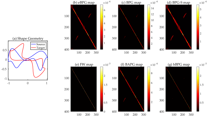
Figure 2: (a): 2D shape geometry of the source and target; (b)-(g): visualization of coupling matrix.

Figs.2 (b)-(g) provide all color maps of coupling matrices to visualize the matching results. Here, the sparser coupling matrices indicate sharper mapping. All experiment results are consistent with Table 1. We can observe that both BPG and FW give us satisfactory solution performance as they aim at solving the GW problem exactly. However, FW and BPG will suffer from a huge computation burden which will be further justified in Sec 4.2 and 4.3. On the other hand, the performance of eBPG, BPG-S and BAPG are obviously harmed by not solving the original GW problem or the infeasibility issue. The sharpness of BAPG’s coupling matrix is relatively not effected by its infeasibility issue too much although its coupling matrix is denser than BPG and FW ones. As we shall see later, the effect of the infeasibility issue is minor when the penalty parameter $\rho$ is not too small and will not even result in even a real cost for graph alignment and partition tasks, which only care about the matching accuracy instead of the sharpness of the coupling. Moreover, the characteristics of eBPG and BPG motivate us to apply hBPG for shape correspondence problems. Instead, BAPG shows its potential for being applied to graph alignment and graph partition tasks, which only care about the matching accuracy instead of the sharpness of the coupling.

4.2 Graph Alignment

Graph alignment aims to identify the node correspondence between two graphs possibly with different topology structures (Zhang et al., 2021; Chen et al., 2020). Instead of solving the restricted quadratic assignment problem (Lawler, 1963; Lacoste-Julien et al., 2006), the GW distance provides the optimal probabilistic correspondence relationship via preservation of the isometric property. Here, we compare the proposed BAPG and hBPG with all existing baselines: FW (Titouan et al., 2019), BPG (Xu et al., 2019b), BPG-S (Xu et al., 2019b) (i.e., the only difference between BPG and BPG-S is that the number of inner iterations for BPG-S is just one), ScalaGW (Xu et al., 2019a), SpecGW (Chowdhury and Needham, 2021), and eBPG (Solomon et al., 2016). Except for BPG and eBPG, others are pure heuristic methods without any theoretical guarantee. Besides the GW-based methods, we also consider three widely used non-GW graph alignment baselines, including IPFP (Leordeanu et al., 2009), RRWM (Cho et al., 2010), and SpecMethod (Leordeanu and Hebert, 2005).

Parameters Setup

We utilize the unweighted symmetric adjacent matrices as our input distance matrices, i.e., $D_{X}$ and $D_{Y}$. Alternatively, SpecGW uses the heat kernel $\exp(-L)$ where $L$ is the normalized graph Laplacian matrix. We set both $\mu$ and $\nu$ to be the uniform distribution. For three heuristic methods — BPG-S, ScalaGW, and SpecGW, we follow the same setup reported in their papers. As mentioned, eBPG is very sensitive to the entropic regularization parameter. To get comparable results, we report the best result among the set $\{0.1,0.01,0.001\}$ of the regularization parameter. For BPG and BAPG, we use the constant step size $5$ and $\rho=0.1$ respectively. For FW, we use the default implementation in the PythonOT package (Flamary et al., 2021).

Table 2: Statistics of databases for graph alignment.

Dataset	# Samples	Ave. Nodes	Ave. Edges
Synthetic	300	1500	56579
Proteins	1113	39.06	72.82
Enzymes	600	32.63	62.14
Reddit	500	375.9	449.3

Table 3: Comparison of the matching accuracy (%) and wall-clock time (seconds) on graph alignment. For BAPG, we also report the time of GPU implementation.

Method	Synthetic		Proteins			Enzymes			Reddit
	Acc	Time	Raw	Noisy	Time	Raw	Noisy	Time	Raw	Noisy	Time
IPFP	-	-	43.84	29.89	87.0	40.37	27.39	23.7	-	-	-
RRWM	-	-	71.79	33.92	239.3	60.56	30.51	114.1	-	-	-
SpecMethod	-	-	72.40	22.92	40.5	71.43	21.39	9.6	-	-	-
FW	24.50	8182	29.96	20.24	54.2	32.17	22.80	10.8	21.51	17.17	1121
ScalaGW	17.93	12002	16.37	16.05	372.2	12.72	11.46	213.0	0.54	0.70	1109
SpecGW	13.27	1462	78.11	19.31	30.7	79.07	21.14	6.7	50.71	19.66	1074
eBPG	34.33	9502	67.48	45.85	208.2	78.25	60.46	499.7	3.76	3.34	1234
BPG	57.56	22600	71.99	52.46	130.4	79.19	62.32	73.1	39.04	36.68	1907
BPG-S	61.48	18587	71.74	52.74	40.4	79.25	62.21	13.4	39.04	36.68	1431
hBPG	51.57	13279	70.07	49.01	245.9	78.57	62.26	560.0	47.15	45.58	1447
BAPG	99.79	9024	78.18	57.16	59.1	79.66	62.85	14.8	50.93	49.45	780
BAPG-GPU	-	1253	-	-	75.4	-	-	21.8	-	-	115

Database Statistics

We test all methods on both synthetic and real-world databases. Our setup for the synthetic database is the same as in (Xu et al., 2019b). The source graph $\mathcal{G}_{s}=\{\mathcal{V}_{s},\mathcal{E}_{s}\}$ is generated by two ideal random models, Gaussian random partition and Barabasi-Albert models, with different scales, i.e., $|\mathcal{V}_{s}|\in\{500,1000,1500,2000,2500\}$. Then, we generate the target graph $\mathcal{G}_{t}=\{\mathcal{V}_{t},\mathcal{E}_{t}\}$ by first adding $q\%$ noisy nodes to the source graph, and then generating $q\%$ noisy edges between the nodes in $\mathcal{V}_{t}$, i.e., $|\mathcal{V}_{t}|=(1+q\%)|\mathcal{V}_{s}|,|\mathcal{E}_{t}|=(1+q\%)|\mathcal{E}_{s}|$, where $q\in\{0,10,20,30,40,50\}$. For each setup, we generate five synthetic graph pairs over different random seeds. To sum up, the synthetic database contains 300 different graph pairs. We also validate our proposed methods on other three real-world databases from (Chowdhury and Needham, 2021), including two biological graph databases Proteins and Enzymes, and a social network database Reddit. Furthermore, to demonstrate the robustness of our method regarding the noise level, we follow the noise generating process (i.e., $q=10\%$) conducted for the synthesis case to create new databases on top of the three real-world databases. Towards that end, the statistics of all databases used for the graph alignment task have been summarized in Table 2. We match each node in $\mathcal{G}_{s}$ with the most likely node in $\mathcal{G}_{t}$ according to the optimized $\pi^{\star}$. Given the predicted correspondence set $\mathcal{S}_{\text{pred}}$ and the ground-truth correspondence set $\mathcal{S}_{\text{gt}}$, we calculate the matching accuracy by $\textnormal{Acc}=|\mathcal{S}_{\text{gt}}\cap\mathcal{S}_{\text{pred}}|/|\mathcal{S}_{\text{gt}}|\times 100\%$.

Results of Our Methods

Table 3 shows the comparison of matching accuracy and wall-clock time on four databases. We observe that BAPG works exceptionally well both in terms of computational time and accuracy, especially for two large-scale noisy graph databases Synthetic and Reddit. Notably, BAPG is robust enough so that it is not necessary to perform parameter tuning. As we mentioned in Sec 2, the effectiveness of GPU acceleration for BAPG is also well corroborated on Synthetic and Reddit. GPU cannot further speed up the training time of Proteins and Reddit as graphs in these two databases are small-scale. Additional experiment results to demonstrate the robustness of BAPG and its GPU acceleration will be given in Sec 4.5. Observed from Table 3, the performance of hBPG is in general the interpolation between eBPG and BPG in terms of modeling performance and wall-clock time.

Comparison with Other Methods

Traditional non-GW graph alignment methods (IPFP, RRWM, and SpecMethod) have the out-of-memory issue on graphs with more than 500 nodes (e.g., Synthetic and Reddit) and are sensitive to the noise. The performance of eBPG and ScalaGW are influenced by the entropic regularization parameter and approximation error respectively, which accounts for their poor performance. Moreover, it is easy to observe that SpecGW works pretty well on the small dataset but the performance degrades dramatically on the large one, e.g., synthetic. The reason is that SpecGW relies on a linear programming solver as its subroutine, which is not well-suited for large-scale settings. Besides, although ScalaGW has the lowest per-iteration computational complexity, the recursive K-partition mechanism developed in (Xu et al., 2019a) is not friendly to parallel computing. Therefore, ScalaGW does not demonstrate attractive performance on multi-core processors.

4.3 Graph Partition

The GW distance can also be potentially applied to the graph partition task. That is, we are trying to match the source graph with a disconnected target graph having $K$ isolated and self-connected super nodes, where $K$ is the number of clusters (Abrishami et al., 2020). Similarly, we compare the proposed BAPG and hBPG with other baselines described in Section 4.2 on four real-world graph partitioning datasets. Following (Chowdhury and Needham, 2021), we also add three non-GW methods specialized in graph alignment, including FastGreedy (Clauset et al., 2004), Louvain (Blondel et al., 2008), and Infomap (Rosvall and Bergstrom, 2008).

Parameters Setup

For the input distance matrices $D_{X}$ and $D_{Y}$, we test our methods on both the adjacent matrices and the heat kernel matrices proposed in (Chowdhury and Needham, 2021). For BAPG, we pick up the lowest converged function value among $\rho\in\{0.1,0.05,0.01\}$ for adjacent matrices and $\rho\in\{0.01,0.005,0.001\}$ for heat kernel matrices. The quality of graph partition results is quantified by computing the adjusted mutual information (AMI) score (Vinh et al., 2010) against the ground-truth partition.

Table 4: Comparison of AMI scores on graph partition datasets using the adjacent matrices and the heat kernel matrices.

Matrices	Method	Wikipedia		EU-email		Amazon		Village
		Raw	Noisy	Raw	Noisy	Raw	Noisy	Raw	Noisy
Non-GW	FastGreedy	0.382	0.341	0.312	0.251	0.637	0.573	0.881	0.778
	Louvain	0.377	0.329	0.447	0.382	0.622	0.584	0.881	0.827
	Infomap	0.332	0.329	0.374	0.379	0.940	0.463	0.881	0.190
Adjacent	FW	0.341	0.323	0.440	0.409	0.374	0.338	0.684	0.539
	eBPG	0.461	0.413	0.517	0.422	0.429	0.387	0.703	0.658
	BPG	0.367	0.333	0.478	0.414	0.412	0.368	0.642	0.575
	BPG-S	0.357	0.285	0.451	0.404	0.443	0.352	0.606	0.560
	hBPG	0.368	0.333	0.527	0.423	0.435	0.387	0.655	0.554
	BAPG	0.468	0.385	0.508	0.428	0.436	0.426	0.709	0.681
Heat Kernel	SpecGW	0.442	0.395	0.487	0.425	0.565	0.487	0.758	0.707
	eBPG	0.000	0.000	0.000	0.000	0.000	0.000	0.000	0.000
	BPG	0.405	0.373	0.473	0.253	0.492	0.436	0.705	0.619
	BPG-S	0.411	0.373	0.475	0.253	0.483	0.425	0.642	0.619
	hBPG	0.497	0.387	0.166	0.059	0.477	0.389	0.782	0.727
	BAPG	0.529	0.397	0.533	0.436	0.609	0.505	0.797	0.711

Results of All Methods

Table 4 shows the comparison of AMI scores among all methods on graph partition. BAPG outperforms other GW-based methods in most cases and is more robust to the noisy setting. Specifically, BAPG is consistently better than FW and SpecGW which both rely on the Frank-Wolfe method to solve the problem. eBPG has comparable results using the adjacency matrices but is unable to process the spectral matrices. The possible reason is that the adjacency matrix and the heat kernel matrix admit quite different structures, e.g., the former is sparse while the latter is dense. The performance of hBPG is in general the interpolation between eBPG and BPG. BPG and BPG-S enjoy similar performances in most cases, but both are not as good as our proposed BAPG on all datasets. Except for BPG and eBPG, others are pure heuristic methods without any theoretical guarantee. BAPG also shows competitive performance compared to the specialized non-GW graph partition methods. For example, BAPG outperforms Infomap in 6 out of 8 scores.

4.4 Shape Correspondence

(a) Source Surface

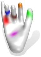
(b) eBPG

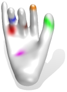
(c) BAPG

(d) BPG

(e) hBPG

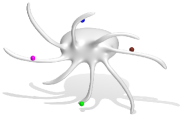
(f) Source Surface

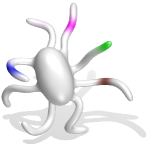
(g) eBPG

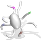
(h) BAPG

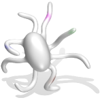
(i) BPG

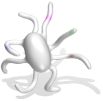
(j) hBPG

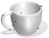
(k) Source Surface

(l) eBPG

(m) BAPG

(n) BPG

(o) hBPG

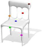
(p) Source Surface

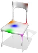
(q) eBPG

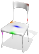
(r) BAPG

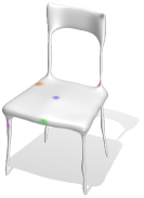
(s) BPG

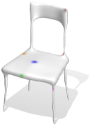
(t) hBPG

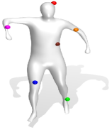
(u) Source Surface

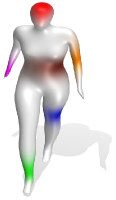
(v) eBPG

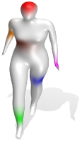
(w) BAPG

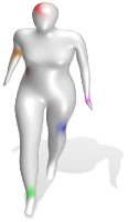
(x) BPG

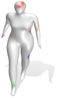
(y) hBPG

Figure 3: Visualization of the matching results: colored points (source surface) are mapped to colored distributions on the target object.

Table 5: Comparison of the infeasibility error (i.e.,$\tfrac{\|\pi^{T}\mathbf{1}_{n}-\nu\|}{m}+\tfrac{\|\pi\mathbf{1}_{m}-\mu\|}{n}$ ) and CPU wall-clock time.

Method	Hand		Octopus		Mug		Chair		Human
	Error	Time	Error	Time	Error	Time	Error	Time	Error	Time
eBPG	2.95e-10	9.37	7.21e-10	12.08	6.41e-10	27.86	1.77e-10	12.87	5.52e-10	11.46
BPG	3.00e-07	389.72	2.00e-07	32.55	3.50e-07	196.93	4.00e-07	304.98	2.53e-07	93.27
hBPG	3.00e-07	193.85	2.00e-07	23.14	3.50e-07	90.59	4.00e-07	189.41	2.53e-07	53.29
BAPG	4.54e-06	61.77	2.14e-05	6.19	6.62e-05	30.83	2.13e-05	127.78	5.62e-05	8.26
BAPG-GPU	-	3.10	-	1.28	-	1.39	-	3.22	-	0.78

Finally, we evaluate the matching performance and computational cost of our proposed hBPG and BAPG on five 3D triangle mesh datasets used in Solomon et al. (2016). By making use of gptoolbox (Jacobson et al., 2018), $D_{X}$ and $D_{Y}$ are constructed by computing the geodesic distances over the triangle mesh. Here, $\mu$ and $\nu$ are discrete uniform distributions. All the algorithmic parameters of eBPG, BPG, BAPG and hBPG have been fine-tuned via grid search for optimal performance.

Different from graph alignment and partition, the shape matching task cares more about the sharpness of the correspondence relationship. To visualize this soft matching result, we label several color points on the source surface and then quantify the sharpness of each mapping distribution via the size of the colored area on the target surface. In fact, the smaller area indicates a sharper mapping. Regarding the accuracy and sharpness, the superiority of hBPG and BPG over other methods are obviously observed from Fig. 3. If we further take the computational burden into account, hBPG is the best-fit for this task, see Table 5 for details. hBPG can achieve a great trade-off between efficiency and accuracy. Although BAPG shows attractive advantages in terms of computational cost, it suffers from the infeasibility issue, which is also corroborated by the experiment results in Table 5. The visualization results of the other four 3D mesh objects are given in Appendix.

4.5 The Effectiveness and Robustness of BAPG

At first, we target at demonstrating the robustness of BAPG on graph alignment, as it would be more reasonable to test the robustness of a method on a database (e.g., graph alignment) rather than a single point (e.g., graph partition).

Noise Level and Graph Scale

At the beginning, we report the sensitivity analysis of BAPG regarding the noise level $q\%$ and the graph scale $|\mathcal{V}_{s}|$ in Fig. 4 on the Synthetic Database. Surprisingly, the solution performance of BAPG is robust to both the noise level and graph scale. In contrast, the accuracy of other methods degrades dramatically as the noise level or the graph scale increases.

Step Size $\rho$

Subsequently, we conduct the sensitivity analysis of BAPG with respect to the step size $\rho$ on four real-world databases. Table 6 showcases that the matching performance of BAPG is stable and robust (not sensitive) regarding the step size. Moreover, convergence curves of different $\rho$ in Fig. 4 corroborate Proposition 3.4 empirically and further guide us on how to choose the step size. The larger $\rho$ means the smaller infeasibility error but slower convergence speed. Together with Table 6, we can conclude that if the resulting infeasibility error is not quite large (i.e., the step size $\rho$ is not so small), the final matching accuracy is robust to the step size. Under this situation, the step size only affects the convergence speed.

Table 6: The sensitivity analysis of BAPG with different step sizes $\rho$ on graph alignment.

Method	Synthetic		Proteins			Enzymes			Reddit
	Acc	Time	Clean	Noise	Time	Clean	Noise	Time	Clean	Noise	Time
BAPG ($\rho$=0.5)	94.58	4610	77.21	57.69	70.8	79.20	63.18	21.8	50.04	49.19	257
BAPG ($\rho$=0.2)	98.87	2074	78.27	57.96	67.4	79.50	63.06	17.6	50.94	50.46	144
BAPG ($\rho$=0.1)	99.79	1253	78.18	57.16	59.1	79.66	62.85	14.8	50.93	49.45	115
BAPG ($\rho$=0.05)	99.20	675	77.59	56.54	32.6	79.27	62.13	11.8	50.96	50.30	98
BAPG ($\rho$=0.01)	93.63	616	60.08	34.47	22.5	66.45	42.38	8.9	28.74	16.14	85

Table 7: GPU & CPU wall-clock time comparison of BAPG, BPG and eBPG on graph alignment.

	Reddit Dataset			Synthetic Dataset
	BAPG	BPG	eBPG	BAPG	BPG	eBPG
CPU Time(s)	780	1907	1234	9024	22600	9502
GPU Time(s)	115	1013	2274	1253	4458	2709
Acceleration Ratio	6.78	1.88	0.54	7.20	5.07	3.51

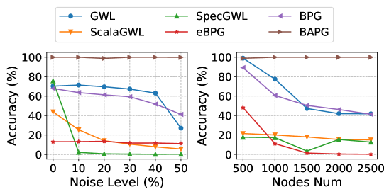
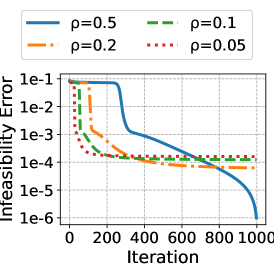
Figure 4: (a) Sensitivity of the noise level and graph scale on the synthetic graph alignment database. (b) Sensitivity of BAPG’s step size $\rho$. The infeasibility error is defined as $\|\pi^{k}-w^{k}\|_{2}$.

GPU Acceleration of BAPG.

We conduct experiment results to further justify that BAPG is GPU-friendly. In Table 7, We compare the acceleration ratio (i.e., CPU wall-clock time divided by GPU wall-clock time) of BAPG, eBPG, and BPG on two large-scale graph alignment datasets using the same computing server. For eBPG, we use the official implementation in the PythonOT package, which supports running on GPU. For BPG, we implement the GPU version by ourselves using Pytorch. We can find that BAPG has a much higher acceleration ratio on the GPU compared with BPG and eBPG.

5 Closing Remark

In this paper, we conduct a systematic investigation on developing provably efficient algorithms for the Gromov-Wasserstein distance computation. Two theoretically solid algorithms, called BAPG and hBPG, have been proposed to tackle different graph learning tasks. Our theoretical results provide novel insights to help users to select the well-suited algorithm for their tasks. Technically, by exploiting the error bound condition (i.e., never investigated in the GW literature before), we are able to conduct the convergence analysis of BAPG (i.e., a special case of alternating projected descent method). For a broader viewpoint, our work also takes the first step and provides a rather new path to study the alternating projected descent method for general nonconvex problems. To the best of our knowledge, it is still an open question even in the optimization community. Unfortunately, the proposed single-loop algorithm BAPG still suffers from the cubic per-iteration computational complexity, which will further limit its applications in real-world large-scale settings. A natural future direction is to consider sparse and low-rank structures of the matching matrix to decrease the per-iteration cost and further speed up our methods (Scetbon et al., 2021). Moreover, for simplicity, we assume that $D_{X}$ and $D_{Y}$ are two symmetric distance matrices. However, the proposed BAPG can be potentially applied to the non-symmetric case as the Luo-tseng error bound condition still holds and algorithmic steps keep the same.

References

- Abrishami et al. (2020) Tara Abrishami, Nestor Guillen, Parker Rule, Zachary Schutzman, Justin Solomon, Thomas Weighill, and Si Wu. Geometry of graph partitions via optimal transport. SIAM Journal on Scientific Computing, 42(5):A3340–A3366, 2020.
- Attouch et al. (2010) Hédy Attouch, Jérôme Bolte, Patrick Redont, and Antoine Soubeyran. Proximal alternating minimization and projection methods for nonconvex problems: An approach based on the kurdyka-łojasiewicz inequality. Mathematics of operations research, 35(2):438–457, 2010.
- Attouch et al. (2013) Hedy Attouch, Jérôme Bolte, and Benar Fux Svaiter. Convergence of descent methods for semi-algebraic and tame problems: proximal algorithms, forward–backward splitting, and regularized gauss–seidel methods. Mathematical Programming, 137(1):91–129, 2013.
- Bauschke et al. (2017) Heinz H Bauschke, Jérôme Bolte, and Marc Teboulle. A descent lemma beyond lipschitz gradient continuity: first-order methods revisited and applications. Mathematics of Operations Research, 42(2):330–348, 2017.
- Beck (2017) Amir Beck. First-order methods in optimization, volume 25. SIAM, 2017.
- Benamou et al. (2015) Jean-David Benamou, Guillaume Carlier, Marco Cuturi, Luca Nenna, and Gabriel Peyré. Iterative bregman projections for regularized transportation problems. SIAM Journal on Scientific Computing, 37(2):A1111–A1138, 2015.
- Blondel et al. (2008) Vincent D Blondel, Jean-Loup Guillaume, Renaud Lambiotte, and Etienne Lefebvre. Fast unfolding of communities in large networks. Journal of statistical mechanics: theory and experiment, 2008(10):P10008, 2008.
- Bunne et al. (2019) Charlotte Bunne, David Alvarez-Melis, Andreas Krause, and Stefanie Jegelka. Learning generative models across incomparable spaces. In International Conference on Machine Learning, pages 851–861. PMLR, 2019.
- Chen et al. (2020) Xiyuan Chen, Mark Heimann, Fatemeh Vahedian, and Danai Koutra. Consistent network alignment via proximity-preserving node embedding. arXiv preprint arXiv:2005.04725, 2020.
- Cho et al. (2010) Minsu Cho, Jungmin Lee, and Kyoung Mu Lee. Reweighted random walks for graph matching. In European conference on Computer vision, pages 492–505. Springer, 2010.
- Chowdhury and Mémoli (2019) Samir Chowdhury and Facundo Mémoli. The gromov–wasserstein distance between networks and stable network invariants. Information and Inference: A Journal of the IMA, 8(4):757–787, 2019.
- Chowdhury and Needham (2021) Samir Chowdhury and Tom Needham. Generalized spectral clustering via gromov-wasserstein learning. In International Conference on Artificial Intelligence and Statistics, pages 712–720. PMLR, 2021.
- Clauset et al. (2004) Aaron Clauset, Mark EJ Newman, and Cristopher Moore. Finding community structure in very large networks. Physical review E, 70(6):066111, 2004.
- Cuturi (2013) Marco Cuturi. Sinkhorn distances: Lightspeed computation of optimal transport. Advances in neural information processing systems, 26:2292–2300, 2013.
- Flamary et al. (2021) Rémi Flamary, Nicolas Courty, Alexandre Gramfort, Mokhtar Z. Alaya, Aurélie Boisbunon, Stanislas Chambon, Laetitia Chapel, Adrien Corenflos, Kilian Fatras, Nemo Fournier, Léo Gautheron, Nathalie T.H. Gayraud, Hicham Janati, Alain Rakotomamonjy, Ievgen Redko, Antoine Rolet, Antony Schutz, Vivien Seguy, Danica J. Sutherland, Romain Tavenard, Alexander Tong, and Titouan Vayer. Pot: Python optimal transport. Journal of Machine Learning Research, 22(78):1–8, 2021. URL http://jmlr.org/papers/v22/20-451.html.
- Gao et al. (2021) Ji Gao, Xiao Huang, and Jundong Li. Unsupervised graph alignment with wasserstein distance discriminator. In Proceedings of the 27th ACM SIGKDD Conference on Knowledge Discovery & Data Mining, pages 426–435, 2021.
- Hanzely et al. (2021) Filip Hanzely, Peter Richtarik, and Lin Xiao. Accelerated bregman proximal gradient methods for relatively smooth convex optimization. Computational Optimization and Applications, 79(2):405–440, 2021.
- Hou et al. (2013) Ke Hou, Zirui Zhou, Anthony Man-Cho So, and Zhi-Quan Luo. On the linear convergence of the proximal gradient method for trace norm regularization. In NIPS, pages 710–718, 2013.
- Jacobson et al. (2018) Alec Jacobson et al. gptoolbox: Geometry processing toolbox. ONLINE: http://github. com/alecjacobson/gptoolbox, 2018.
- Jaggi (2013) Martin Jaggi. Revisiting frank-wolfe: Projection-free sparse convex optimization. In International Conference on Machine Learning, pages 427–435. PMLR, 2013.
- Krichene et al. (2015) Walid Krichene, Syrine Krichene, and Alexandre Bayen. Efficient bregman projections onto the simplex. In 2015 54th IEEE Conference on Decision and Control (CDC), pages 3291–3298. IEEE, 2015.
- Lacoste-Julien (2016) Simon Lacoste-Julien. Convergence rate of frank-wolfe for non-convex objectives. arXiv preprint arXiv:1607.00345, 2016.
- Lacoste-Julien et al. (2006) Simon Lacoste-Julien, Ben Taskar, Dan Klein, and Michael Jordan. Word alignment via quadratic assignment. 2006.
- Lawler (1963) Eugene L Lawler. The quadratic assignment problem. Management science, 9(4):586–599, 1963.
- Leordeanu and Hebert (2005) Marius Leordeanu and Martial Hebert. A spectral technique for correspondence problems using pairwise constraints. In International Conference on Computer Vision, pages 1482–1489. IEEE, 2005.
- Leordeanu et al. (2009) Marius Leordeanu, Martial Hebert, and Rahul Sukthankar. An integer projected fixed point method for graph matching and map inference. Advances in neural information processing systems, 22, 2009.
- Li and Pong (2018) Guoyin Li and Ting Kei Pong. Calculus of the exponent of Kurdyka-Łojasiewicz inequality and its applications to linear convergence of first-order methods. Foundations of Computational Mathematics, 18(5):1199–1232, 2018.
- Li et al. (2020) Xudong Li, Defeng Sun, and Kim-Chuan Toh. On the efficient computation of a generalized jacobian of the projector over the birkhoff polytope. Mathematical Programming, 179(1-2):419–446, 2020.
- Luo and Tseng (1992) Zhi-Quan Luo and Paul Tseng. Error bound and convergence analysis of matrix splitting algorithms for the affine variational inequality problem. SIAM Journal on Optimization, 2(1):43–54, 1992.
- Mai et al. (2021) Vien V Mai, Jacob Lindbäck, and Mikael Johansson. A fast and accurate splitting method for optimal transport: Analysis and implementation. arXiv preprint arXiv:2110.11738, 2021.
- Mémoli (2009) Facundo Mémoli. Spectral gromov-wasserstein distances for shape matching. In 2009 IEEE 12th International Conference on Computer Vision Workshops, ICCV Workshops, pages 256–263. IEEE, 2009.
- Mémoli (2011) Facundo Mémoli. Gromov–wasserstein distances and the metric approach to object matching. Foundations of computational mathematics, 11(4):417–487, 2011.
- Mémoli (2014) Facundo Mémoli. The gromov–wasserstein distance: A brief overview. Axioms, 3(3):335–341, 2014.
- Mémoli and Sapiro (2004) Facundo Mémoli and Guillermo Sapiro. Comparing point clouds. In Proceedings of the 2004 Eurographics/ACM SIGGRAPH symposium on Geometry processing, pages 32–40, 2004.
- Nedić (2011) Angelia Nedić. Random algorithms for convex minimization problems. Mathematical programming, 129(2):225–253, 2011.
- Nocedal and Wright (2006) Jorge Nocedal and Stephen Wright. Numerical optimization. Springer Science & Business Media, 2006.
- Peyré et al. (2016) Gabriel Peyré, Marco Cuturi, and Justin Solomon. Gromov-wasserstein averaging of kernel and distance matrices. In International Conference on Machine Learning, pages 2664–2672. PMLR, 2016.
- Peyré et al. (2019) Gabriel Peyré, Marco Cuturi, et al. Computational optimal transport: With applications to data science. Foundations and Trends® in Machine Learning, 11(5-6):355–607, 2019.
- Rosvall and Bergstrom (2008) Martin Rosvall and Carl T Bergstrom. Maps of random walks on complex networks reveal community structure. Proceedings of the national academy of sciences, 105(4):1118–1123, 2008.
- Scetbon et al. (2021) Meyer Scetbon, Gabriel Peyré, and Marco Cuturi. Linear-time gromov wasserstein distances using low rank couplings and costs. arXiv preprint arXiv:2106.01128, 2021.
- Séjourné et al. (2021) Thibault Séjourné, François-Xavier Vialard, and Gabriel Peyré. The unbalanced gromov wasserstein distance: Conic formulation and relaxation. Advances in Neural Information Processing Systems, 34:8766–8779, 2021.
- Solomon et al. (2016) Justin Solomon, Gabriel Peyré, Vladimir G Kim, and Suvrit Sra. Entropic metric alignment for correspondence problems. ACM Transactions on Graphics (TOG), 35(4):1–13, 2016.
- Titouan et al. (2019) Vayer Titouan, Nicolas Courty, Romain Tavenard, and Rémi Flamary. Optimal transport for structured data with application on graphs. In International Conference on Machine Learning, pages 6275–6284. PMLR, 2019.
- Vayer et al. (2018) Titouan Vayer, Laetita Chapel, Rémi Flamary, Romain Tavenard, and Nicolas Courty. Fused gromov-wasserstein distance for structured objects: theoretical foundations and mathematical properties. arXiv preprint arXiv:1811.02834, 2018.
- Vayer et al. (2019) Titouan Vayer, Rémi Flamary, Romain Tavenard, Laetitia Chapel, and Nicolas Courty. Sliced gromov-wasserstein. In NeurIPS 2019-Thirty-third Conference on Neural Information Processing Systems, volume 32, 2019.
- Vincent-Cuaz et al. (2021a) Cédric Vincent-Cuaz, Rémi Flamary, Marco Corneli, Titouan Vayer, and Nicolas Courty. Semi-relaxed gromov wasserstein divergence with applications on graphs. arXiv preprint arXiv:2110.02753, 2021a.
- Vincent-Cuaz et al. (2021b) Cédric Vincent-Cuaz, Titouan Vayer, Rémi Flamary, Marco Corneli, and Nicolas Courty. Online graph dictionary learning. arXiv preprint arXiv:2102.06555, 2021b.
- Vinh et al. (2010) Nguyen Xuan Vinh, Julien Epps, and James Bailey. Information theoretic measures for clusterings comparison: Variants, properties, normalization and correction for chance. The Journal of Machine Learning Research, 11:2837–2854, 2010.
- Wang and Bertsekas (2016) Mengdi Wang and Dimitri P Bertsekas. Stochastic first-order methods with random constraint projection. SIAM Journal on Optimization, 26(1):681–717, 2016.
- Xu et al. (2019a) Hongteng Xu, Dixin Luo, and Lawrence Carin. Scalable gromov-wasserstein learning for graph partitioning and matching. Advances in neural information processing systems, 32:3052–3062, 2019a.
- Xu et al. (2019b) Hongteng Xu, Dixin Luo, Hongyuan Zha, and Lawrence Carin Duke. Gromov-wasserstein learning for graph matching and node embedding. In International conference on machine learning, pages 6932–6941. PMLR, 2019b.
- Xu et al. (2021) Hongteng Xu, Dixin Luo, Lawrence Carin, and Hongyuan Zha. Learning graphons via structured gromov-wasserstein barycenters. In Proceedings of the AAAI Conference on Artificial Intelligence, volume 35, pages 10505–10513, 2021.
- Xu et al. (2022) Hongteng Xu, Jiachang Liu, Dixin Luo, and Lawrence Carin. Representing graphs via gromov-wasserstein factorization. IEEE Transactions on Pattern Analysis and Machine Intelligence, 2022.
- Zhang and Luo (2022) Jiawei Zhang and Zhi-Quan Luo. A global dual error bound and its application to the analysis of linearly constrained nonconvex optimization. SIAM Journal on Optimization, 32(3):2319–2346, 2022.
- Zhang et al. (2021) Si Zhang, Hanghang Tong, Long Jin, Yinglong Xia, and Yunsong Guo. Balancing consistency and disparity in network alignment. In Proceedings of the 27th ACM SIGKDD Conference on Knowledge Discovery & Data Mining, pages 2212–2222, 2021.
- Zhou and So (2017) Zirui Zhou and Anthony Man-Cho So. A unified approach to error bounds for structured convex optimization problems. Mathematical Programming, 165(2):689–728, 2017.