Micromagnets dramatically enhance effects of viscous hydrodynamic flow in two-dimensional electron fluid

Abstract

The hydrodynamic behavior of electron fluids in a certain range of temperatures and densities is well established in graphene and in 2D semiconductor heterostructures. The hydrodynamic regime is intrinsically based on electron-electron interactions, and therefore it provides a unique opportunity to study electron correlations. Unfortunately, in simple longitudinal resistance measurements, the relative contribution of hydrodynamic effects to transport is rather small, especially at higher temperatures. Viscous hydrodynamic effects are masked by impurities, interaction with phonons, uncontrolled boundaries and ballistic effects. This essentially limits the accuracy of measurements of electron viscosity. Fundamentally, what causes viscous friction in the electron fluid is the property of the flow called vorticity. In this paper, we propose to use micromagnets to increase the vorticity by orders of magnitude. Experimental realization of this proposal will bring electron hydrodynamics to a qualitatively new precision level, as well as opening a new way to characterize and externally control the electron fluid.

I Introduction

Viscous hydrodynamic flow of the electron fluid, first postulated by Gurzhi over half a century ago,[1] is now well established experimentally. [2] In the hydrodynamic regime, the momentum conserving electron-electron scattering timescale is much shorter than the momentum relaxation timescale related to impurities and phonons, allowing neighboring electrons to establish local thermal equilibrium such that the flow behaves as a fluid. This condition requires samples of very high purity, therefore the theoretical predictions of the hydrodynamic regime in the 1960s [1, 3] could only be realized experimentally after the advent of high mobility semiconductors [4] and graphene. [5, 2] The opposite side of the story is that the relative contribution of viscous hydrodynamic effects to transport is bounded even in modern high mobility samples, which drastically limit the precision of all the existing measurements of viscosity. In this work, we propose a way to overcome this limitation.

The hydrodynamic nature of the electron flow manifests itself in a number of phenomena that have been demonstrated in recent studies. While the hydrodynamic regime was first thought to be experimentally realized in 1995 in Ref.[4], this interpretation of the results was challenged in the same year in Ref.[6], as the requirements for viscous hydrodynamics in a two-dimensional material differs from that in three-dimensions. Reliable evidence of the hydrodynamic regime was first presented two decades later in Refs.[7, 8, 9]. Notable consequences of hydrodynamic behavior are: the decrease of resistance with increasing temperature known as the Gurzhi effect,[4, 10, 11, 12, 13, 14] Poiseuille flow profiles, [15, 16, 17] negative non-local resistance and formation of whirlpools, [18, 19, 7, 20] Hall viscosity, [13, 21] negative magnetoresistance, [22, 23, 12, 24, 9, 25] the violation of the Wiedemann-Franz law, [26, 27, 28, 29, 30] anomalous scaling of resistance with channel width, [27, 8], resonant photoresistance in magnetic field [31, 32, 33, 34, 25] and quantum-critical dynamic conductivity. [35] Furthermore, many novel phenomena have been proposed, including the elimination of Landauer-Sharvin resistance, [36] anisotropic fluids, [37, 38] dynamo effect in the electron-hole plasma [39] and most excitingly the prospect of hydrodynamic spin transport [40, 41, 42] inspired by experiments on liquid mercury. [43, 44] So far almost all experiments in the field have been aimed at a qualitative demonstration of various hydrodynamic effects. Extraction of quantitative information has been hindered by the weakness of the contribution of hydrodynamics effects to electron transport. The quantitative information is important for understanding correlation effects and it is essential for future technological applications of the electron fluid.

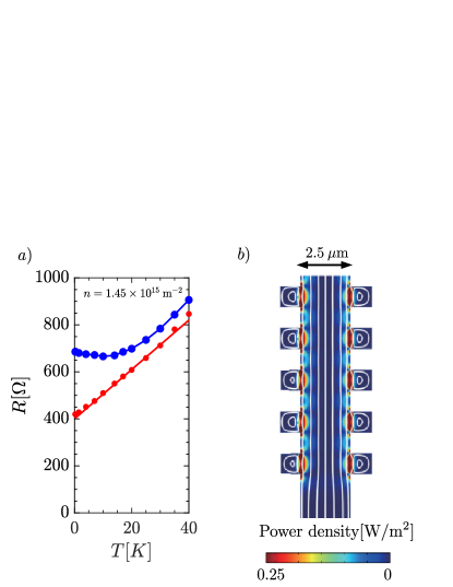
Figure 1: a) Resistivity of the GaAs device from Ref. [12] versus temperature. The red line represents the ohmic resistance and the blue line represents the total (ohmic plus viscous) resistance. b) The map of the viscous dissipation (proportional to vorticity) in the device (drawn to scale). Vorticity is concentrated around sharp corners and practically absent in the bulk.

In the hydrodynamic regime, the flow of electrons is characterized by the viscosity of the electron fluid. Hydrodynamic flow of electrons may be analyzed using the methods of classical fluid mechanics, particularly solving the Navier-Stokes equations. [45] While the flow is classical, the viscosity of the electron fluid is determined by electron-electron scattering that is purely quantum mechanical. Therefore, precise measurements of viscosity provides a new way to study electron-electron correlations. [46] The most precise measurements of the viscosity of electron fluid in 2D GaAs heterostructure [12] to date indicate deviations from predictions of RPA and improved RPA Hubbard theory (See also Ref. [25, 46]). To study this deviation from theory and fully characterize and control the electron fluid, one needs an effective and precise method to measure viscosity.

To explain the limitations of the existing viscosity measurements in Fig. 1 we copy two figures from Ref. [12]. Simply, the red line in Fig. 1a approximately represents the ohmic resistance (scattering from impurities and phonons) and the blue line represents the total (ohmic plus viscous) resistance. At low temperatures, $T\lesssim 20-25$K the difference between the ohmic and total resistance is significant, but this is a manifestation of the transition from the ballistic to the hydrodynamic regime. The transition itself is an interesting problem, see Ref. [11], but it is not directly relevant to the hydrodynamic regime, which is realized at $T\gtrsim 20-25$K in this sample. In the hydrodynamic regime in this sample, the electron-electron scattering length is $l_{ee}\sim 100$ nm and the impurity-phonon scattering length is $l_{imp/ph}\gtrsim 5\>\mu$m. While the hydrodynamic regime is realised as $l_{ee}\ll l_{imp/ph}$, according to Fig. 1a, the relative contribution of the viscous dissipation is approximately 10% of the ohmic contribution, a relatively small contribution. The suppression is easy to understand: the ohmic dissipation exists throughout the sample, while the viscous dissipation comes only from the region near the boundaries [45, 47, 48] that contain non-zero vorticity. This vorticity is generated by obstacles, [49, 50] inhomogeneities in the geometry [51, 12] or rough channel walls. [15] Boundary layers have width $\sim D=\sqrt{l_{ee}l_{imp/ph}/4}$ and constitute a small fraction of the total volume, as shown in Fig. 1b. While this example is specific to the experiment in Ref. [12], to the best of our knowledge the issue of the low vorticity is relevant to all existing measurements in graphene and in semiconductors.

The idea of the present work is to create an oscillatory flow pattern, or “zigzag” flow, schematically shown in

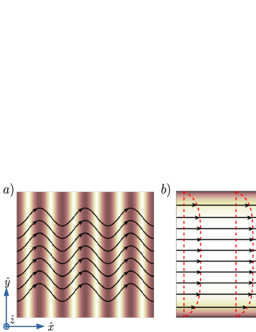
Figure 2: Velocity field $\mathbf{v}$ (arrows) and streamlines (solid black lines) in a) the “zigzag” flow versus b) in ordinary flow inside a no-slip channel, where tangential velocity is zero at the boundaries. In (b) the velocity is purely horizontal and is uniform in the bulk, but the magnitude decays to zero near the no-slip boundaries, forming a non-uniform profile (red dashed lines). Therefore, the strength of vorticity $|\hat{z}\cdot\nabla\times\mathbf{v}|$ (normalized and shown by pink shade) is distributed throughout the bulk in (a), whereas in (b) it is exponentially small except in the boundary layers.

Fig. 2. In the flow through a channel with non-uniform or rough boundaries, a profile develops that is schematically illustrated by the dashed red lines shown in Fig. 2. In such a conventional flow, vorticity is limited to regions near the boundaries of the channel. On the contrary, the solid black oscillatory streamlines in Fig. 2 carry a uniform vorticity throughout the bulk area, and hence the viscous dissipation can match or exceed the ohmic dissipation.

Periodic geometric modulation or obstacles, create boundary layers near geometric features which decay into the bulk [49, 12] (see for example red regions in Fig. 1b). Therefore, the “zigzag” flow in the bulk cannot be established through geometric modulation. However, this non-decaying “zigzag” flow profile may be generated using micromagnets that produce a spatially non-uniform magnetic field of amplitude in the range $20$-$30$ mT, that permeates the bulk. The spatial period of the magnetic field must be of the order of a few $\mu$m, similar to the characteristic viscous length scale. In principle, the idea of the oscillatory flow is equally applicable to the two-dimensional electron gas (2DEG) in both semiconductor quantum wells and graphene. However, boundary conditions that reconcile the oscillatory flow with flat boundaries are significantly different for these two cases. In this paper, we consider the semiconductor 2DEG in a straight channel with no-stress boundary condition.

The structure of the paper is as follows. In Section II we solve the Stokes equation exactly for an infinitely wide 2D flow channel with a sinusoidally modulated perpendicular magnetic field. The direction of modulation coincides with the direction of the flow. This allows us to calculate the viscous and the ohmic dissipation rates and to show that the ratio of viscous to ohmic dissipation can be tuned to become large. Any realistic flow channel has a finite width, therefore in Section III we study the boundary layer in a straight channel using the no-stress boundary condition. Through this solution we find the flow inside the boundary layer. Since the boundary layer problem is the most mathematically delicate issue, we solve the problem by two different methods, (i) perturbation theory, (ii) exact numerical solution. The central result of Section III is the width of the boundary layer. This proves that the “zigzag” flow can be realized in a sufficiently wide straight channel and allows the determination of an appropriate channel width. In Section IV we calculate the magnetic field of periodic ferromagnetic stripes and hence determine parameters of micromagnets necessary for the experimental set up. Section  V presents our conclusions.

II Flow in infinitely wide and infinitely long 2D channel

We consider low currents in the 2DEG, corresponding to low Reynolds number flow. Therefore, we will neglect the Navier term, $\mathbf{v}\cdot\nabla\mathbf{v}$, in the Navier-Stokes equation as it is quadratic in velocity. The flow is also incompressible as the charge carrier density in the 2DEG is controlled via the top gate voltage. Furthermore, we assume steady flow has been established in the channel. The resulting stationary Stokes equation for a two-dimensional incompressible electron fluid in a magnetic field reads  [45]

$$\mathbf{v}/\tau-\nu\nabla^{2}\mathbf{v} =-\nabla\Phi/m^{*}+q/m^{*}\mathbf{v}\times\mathbf{B},$$

$$\nabla\cdot\mathbf{v} =0.$$ (1)

Here $\mathbf{v}$ is the fluid velocity, $\nu$ is the kinematic viscosity, $\tau$ is the relaxation time related to ohmic processes (scattering from impurities and phonons), $\Phi$ is the electro-chemical potential, $q$ is the charge of the fluid particle, $m^{*}$ is the effective hydrodynamic mass and $\mathbf{B}$ is the magnetic field. The magnetic field perpendicular to the plane of the 2DEG is periodically modulated along the flow as

$$B=B_{z} =B_{0}b(x),$$

$$b(x) =\sin(gx),$$

$$g =\frac{2\pi}{a}.$$ (2)

For electrons in GaAs, considered in the present paper, the mass $m^{*}$ is just the band structure mass, $m^{*}\approx 0.067m_{e}$. Using the no-stress boundary condition method developed in Ref.[12] the relaxation time $\tau$ can be measured independently of hydrodynamics. $\tau$ is a known phenomenological function of temperature. It is convenient to relate the viscosity and the relaxation time to the electron-electron scattering length $l_{ee}$ and to the electron mean free path $l_{mfp}$.

$$\nu =\frac{1}{4}v_{F}l_{ee},$$

$$\tau =\frac{l_{mfp}}{v_{F}}.$$ (3)

The relations (II) are well known at low temperatures, $T\ll\epsilon_{F}$, where $\epsilon_{F}$ is the Fermi energy. We extend (II) to higher temperatures, $T\sim\epsilon_{F}$, using these relations as definitions of the corresponding lengths, where we use the Fermi velocity $v_{F}$ defined at zero temperature,

$$v_{F}=\frac{p_{F}}{m^{*}}=\frac{\sqrt{2\pi n}}{m^{*}}.$$ (4)

Here $n$ is the number density of the 2DEG and $p_{F}$ is the Fermi momentum.

The viscosity depends on magnetic field [9] as,

$$\nu\propto\frac{1}{1+(B/B^{*})^{2}}.$$ (5)

Here, $B^{*}$ is the characteristic magnetic field of the material, related to the electron-electron scattering length by $B^{*}={p_{F}}/{(2|e|l_{ee})}$. [9] Although this suppression of viscosity by the magnetic field can be incorporated in our analysis, we consider very weak fields, $B\sim B^{*}/10$, so we disregard the $B$-dependence of $\nu$.

To solve Eq. (II) it is convenient to use the stream function, $\psi$, defined as

$$v_{x} =\partial_{y}\psi,$$

$$v_{y} =-\partial_{x}\psi,$$ (6)

which ensures that $\nabla\cdot\mathbf{v}=0$. Acting on Eq (II) with the curl operator $\nabla\times$, and using the definition Eq. (II), we obtain

$$-\nabla^{2}\psi+D^{2}\nabla^{4}\psi =\omega\tau(\partial_{x}b)\partial_{y}\psi,$$ (7a)

$$\omega=\frac{|q|B_{0}}{m^{*}}, \quad D=\sqrt{\nu\tau}=\frac{1}{2}\sqrt{l_{ee}l_{mfp}}.$$ (7b)

We first consider an applied current density $\mathbf{J}=qnv_{0}\hat{x}$ that passes through a very large system and find

$$\psi_{\infty}=v_{0}\left(y+\frac{\omega\tau}{g(1+D^{2}g^{2})}\cos(gx)\right),$$ (8)

where the subscript $\infty$ indicates that this is the solution when system width and length tend to infinity. Indeed, the stream function in Eq. 8 generates the zigzag flow shown in Fig. 2. Note that if the magnetic field has many Fourier components, $b(x)=\sum_{n=1}^{\infty}[\alpha_{n}\sin(ngx)+\beta_{n}\cos(ngx)]$, the generalization of Eq.  (8) is straightforward.

Instead of determining the relationship between electrochemical potential and current from Eq. (II), we can infer the resistance in the system by accounting for the total power dissipation. The terms $m^{*}\mathbf{v}/\tau$ and $-m^{*}\nu\nabla^{2}\mathbf{v}$ in Eq. (II) are respectively the ohmic drag and viscous friction forces in the system. Therefore, the force velocity product gives the corresponding dissipation rates which follow from Eqs. (II) and (8) as

$$\frac{\dot{E}_{\Omega}}{LW}=\frac{nm^{*}}{LW\tau}\int d^{2}rv^{2}=\frac{nm^{*}v_{0}^{2}}{\tau}\ \left(1+\frac{\omega^{2}\tau^{2}}{2(1+D^{2}g^{2})^{2}}\right),$$

$$\frac{\dot{E}_{\nu}}{LW}=\frac{-nm^{*}\nu}{LW}\int d^{2}r{\bm{v}}\cdot\nabla^{2}{\bm{v}}=\frac{nm^{*}v_{0}^{2}}{2\tau}\ \left(\frac{gD\omega\tau}{1+D^{2}g^{2}}\right)^{2}.$$ (9)

Here $L$ and $W$ are the length and the width of the channel respectively.

We may tune free parameters to maximize the ratio $\dot{E}_{\nu}/\dot{E}_{\Omega}$ such that viscous transport is not overshadowed by ohmic effects. It is easy to check that at a fixed value of $\omega\tau$ the ratio is maximum at the following value of $gD$

$$t=\omega\tau,$$

$$gD=[1+t^{2}/2]^{1/4},$$

$$R=\frac{\dot{E}_{\nu}}{\dot{E}_{\Omega}}=\frac{t^{2}}{4(1+\sqrt{1+t^{2}/2})}.$$ (10)

At large magnetic field the ratio grows linearly with amplitude of the magnetic field, $R\approx\omega\tau/(2\sqrt{2})$. However, to avoid the influence of the magnetic field on the viscosity, Eq. (5), we need $B_{0}\ll B^{*}$. This means that the optimization of parameters depends on the value of the relaxation time $\tau$ that is related to the mobility of the 2DEG.

We make realistic estimates for the effect of periodic magnetic field on the GaAs system from Ref. [12]. In order to pick the optimum value for the period of the magnetic superlattice, we first determine $\omega\tau$ from the experimentally measured parameters of the 2DEG. At $T=30-40$K and density $n\sim few\times 10^{11}\>\text{cm}^{-2}$ has $B^{*}\approx 200-250$mT, $\tau\approx 0.3\times 10^{-10}$s and the corresponding mean free path $l_{mfp}\approx 7\mu$m. If we take $B_{0}=30$ mT the $B^{*}$ correction in Eq. (5) to $\nu$ at the peak magnetic field strength is approximately 2% and can be safely neglected. With these values of $B_{0}$ and $\tau$ we find $\omega\tau=2.4$ and hence according to Eq. (II) the ratio is $R\approx 0.5$. Hence, we achieve almost an order of magnitude enhancement of the viscous dissipation compared to Fig. 1a. The value of the characteristic length $D$ defined in Eq. (7a) is $D\approx 0.6\mu$m. Finally, according to Eq. (II) the optimal period of the magnetic superlattice is $a=2\pi/g\approx 2.6\>\mu$m.

III Boundary layer for a straight channel with no-stress boundary condition

In the previous section we considered an infinite fluid domain. Of course, any physical channel must have some finite width $W$. Here we consider a straight channel with no-stress boundary conditions engineered experimentally in Ref. [12]. To support the message of the previous section, we seek to prove that the boundary layer that reconciles the oscillatory bulk flow with the straight flow near the boundary is of a finite width. In other words, the width of the boundary layer must remain finite as the amplitude of magnetic field is increased. Because of the importance of this assertion, we check it by two different methods, (i) analytic solution using perturbation theory in magnetic field, and (ii) exact numerical solution.

III.1 Perturbation theory for the boundary layer flow

For the purpose of deriving an analytic expression for the boundary, we consider the boundary region as a semi-infinite channel with domain $y>0$ and a perfect-slip boundary at $y=0$. Together with the Stokes equation, Eq. (7a), the stream function must satisfy the no-penetration and perfect-slip, or no-stress, boundary conditions as follows, respectively,

$$v_{y}|_{y=0}=-\partial_{x}\psi|_{y=0}=0,\;\partial_{y}v_{x}|_{y=0}=\partial_{y}^{2}\psi|_{y=0}=0.$$ (11)

The former, no-penetration condition ensures no fluid can enter/exist through the boundary. Whereas the latter no-stress condition ensures that the fluid experiences no friction from the boundary, in other words the perfect-slip condition is realized. Furthermore, the stream function must decay to the bulk solution (8) far from the boundary. We look for a solution as an expansion in the powers of $\omega\tau\ll 1$, $\psi=\sum_{n=0}^{\infty}(\omega\tau)^{n}\psi^{(n)}$. Straightforward substitution in Eqs. (7a),and  (11) gives the following 1st order solution

$$\psi = v_{0}\left\{\left(y+\frac{\omega\tau}{g(1+g^{2}D^{2})}\cos(gx)\right)\right.$$

$$+ \left.\frac{\omega\tau}{g}\left(\frac{g^{2}D^{2}}{1+g^{2}D^{2}}e^{-\sqrt{g^{2}D^{2}+1}y/D}-e^{-gy}\right)\cos(gx)\right\}.$$

Due to the optimization condition (II) the wave vector is $g>1/D$, therefore the boundary layer part of the solution (III.1) decays faster than the characteristic length $D$. In Appendix  A we present the expansion of the solution to $\psi$ to the second order in $\omega\tau$ to demonstrate that the effective width of higher order contributions to the boundary decreases with increasing order. The corrections to $\psi$ to second order in $\omega\tau$ part has boundary layer terms that exponentially decay with $y$ at the same rate as that in Eq. (III.1) or faster. Fig. 3 presents plots of streamlines obtained in the 1st and the 2nd order perturbation theory at $\omega\tau=0.5,1$ and $gD=1$.

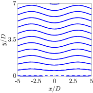
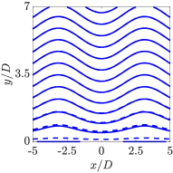
Figure 3: Streamlines for $gD=1$ and $\omega\tau=0.5$ (left) and $\omega\tau=1$ (right). Solid lines correspond to the 1st order perturbation theory and dashed lines correspond to the 2nd order perturbation theory. In both cases the dashed lines almost exactly coincide with the solid lines for $y>D$.

The difference between the solid and the dashed lines in Fig. 3 characterize the convergence of the perturbation theory. While at $\omega\tau=0.5$ there is practically no visible difference between the first and second order perturbation theory, the difference is visible when $\omega\tau=1$. In both cases the boundary layer has almost entirely decayed for $y>2D$, with the flow indistinguishable from the bulk solution given by Eq. (8).

The perturbation theory at $\omega\tau=1$ does not satisfy the small $\omega\tau$ limit and it is hardly possible to justify the perturbation theory at $\omega\tau\approx 3$ corresponding to the optimal device. Therefore, in the following subsection we present the numerical solution valid at arbitrary $\omega\tau$.

III.2 Exact numerical solution for the boundary layer flow

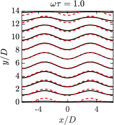
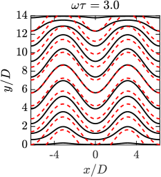
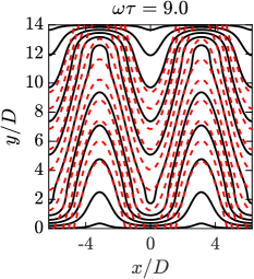
Figure 4: Streamlines in a channel with no-stress boundaries with width $W=14D$. The parameters of the magnetic field are chosen as $gD=1$, $\omega\tau=1,3,9$. Solid lines correspond to the numerically exact solution described in Sec. III.2 and dashed lines correspond to the solution given by Eq. (8) in the infinite device.

In this section, we reduce the Stokes equation, Eq. (7a), to an infinite sequence of linear algebraic equations. We then numerically solve these equations by truncating them at a suitable order. We consider an infinitely long channel of width $W$ and use length units where $D=\sqrt{\nu\tau}=1$. As the magnetic field is periodic in the $x$-direction so is the stream function, $\psi$, which can be presented as the following Fourier series,

$$\psi=v_{0}y+v_{0}W\sum_{m=-\infty}^{\infty}e^{igmx}G_{m}(y)\ .$$ (13)

Here $G_{m}(y)$ are unknown functions to be determined. The first term $v_{0}y$ corresponds to the uniform velocity $v_{x}=v_{0}\neq 0,\>v_{y}=0$.

At $y=0$ and, $y=W$ the stream function must satisfy the no-penetration and no-stress boundary conditions, previously given for $y=0$ in Eq. (11). The no-penetration condition implies that $G_{m}(0)=G_{m}(W)=0$. Hence, the functions $G_{m}(y)$ can be expanded in a Fourier series in $\sin\left(ny\pi/W\right)$ as

$$\psi/v_{0}=y+W\sum_{n=1}^{\infty}\sum_{m=-\infty}^{\infty}f_{m,n}e^{igmx}\sin\left(\frac{ny\pi}{W}\right),$$ (14)

where $f_{m,n}$ are complex coefficients. Note that, this form is chosen so that the no-stress condition is automatically satisfied. Furthermore, the sinusoidal terms do not contribute to the average current through the channel. The Navier-Stoke’s equation, Eq. 7a, expressed in terms of the coefficients $f_{m,n}$ reads

$$\sum_{n=1}D_{m,n}f_{m,n}\sin(ny\pi/W)=\frac{\alpha}{2}\bigg{(}\delta_{m,1}+\delta_{m,-1}\\ +\sum_{n=1}\left[f_{m+1,n}+f_{m-1,n}\right]n\pi\cos(ny\pi/W)\bigg{)},$$ (15)

where $\alpha=-\omega\tau g/W$ and

$$D_{m,n}=-\left[\left(mg\right)^{2}+\left(\frac{\pi n}{W}\right)^{2}\right]\left[\left(mg\right)^{2}+\left(\frac{\pi n}{W}\right)^{2}+1\right].$$ (16)

Eq. (15) is defined only at $0<y<W$. Therefore, one cannot naively equate the Fourier components. Instead we must integrate over $y$ using the following identities

$$\int_{0}^{1}dy\>\sin(ny\pi)\sin(ly\pi)=\frac{1}{2}\delta_{n,l},$$

$$\int_{0}^{1}dy\>\cos(ny\pi)\cos(ly\pi)=\frac{1}{2}\delta_{n,l},$$

$$\int_{0}^{1}dy\>\sin(ny\pi)\cos(ly\pi)=F(n,l),$$

$$F(n,l)=\left\{\begin{array}[]{ccc}0&,&n+l=even\\ \frac{2n}{\pi(n^{2}-l^{2})}&,&n+l=odd.\end{array}\right.$$ (19)

Hence, Eq.( 15) is reduced to the following system of linear algebraic equations for the coefficients $f_{m,l}$:

$$\begin{split}D_{m,l}f_{m,l}={\alpha}&\bigg{(}\sum_{n=1}^{\infty}\left[f_{m+1,n}+f_{m-1,n}\right]n\pi F(l,n)\\ &+(\delta_{m,1}+\delta_{m,-1})F(l,0)\bigg{)},\>l>0,\end{split}$$ (20a)

$$\begin{split}\sum_{n=1}^{\infty}D_{m,n}f_{m,n}&F(n,l)=\frac{\alpha}{4}\bigg{(}\left[f_{m+1,l}+f_{m-1,l}\right]l\pi\\ &+\left[f_{m+1,n}+f_{m-1,n}\right]\delta_{l,0}\bigg{)},\>l\geq 0.\end{split}$$ (20b)

We truncate beyond $|m|,l,n>50$. With a channel width $W=14$ the truncation implies spatial uncertainty $\sim 14/50\approx 0.3$, which is accurate enough to describe the boundary layer.

Plots of the streamlines obtained from this numerical solution for $gD=1$ and $\omega\tau=1,3,9$ are presented in Fig. 4.

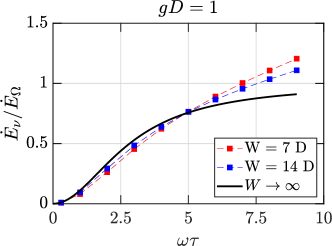
Figure 5: The ratio of viscous to ohmic dissipation at $gD=1$. For the infinite system (solid black line), this ratio is calculated from Eq. (II). For a system with finite width, $W=7D$ (red dots) and $W=14D$ (blue dots), it is calculated from the numerical solution in Sec. III.2. Finite width (boundary layer) effects are negligible when $W\gg 2D$ below $\omega\tau\lesssim 6$.

The exact solution demonstrates that the width of the boundary layer increases with increasing magnetic field. For the most interesting case, $\omega\tau\approx 3$ the width of the boundary layer is about $2D$. The fact that the boundary layers are growing in size with $\omega\tau$ is also evident in Fig. 5. We compare the ratio of viscous to ohmic dissipation in an infinite channel, as calculated in Eq. (II), to a finite width channel. In Fig. 5, the ratio calculated from the exact solution approaches that of an infinite system as the channel width grows, as expected. Of course, for small values of $\omega\tau<1$, the thin boundary layers, as in Fig. 4, have vanishing stress that reduces viscous dissipation. More interestingly, the finite width corrections become noticeable at large $\omega\tau$, where the boundary layer width $2D$ is comparable to the width $W$. Hence, the width of the channel $W$ must be significantly larger than $2D$ for boundary layer effects to be small. For GaAs with mobility of about $10^{6}$ corresponding to the device from Ref. [12] this implies that $W\gg 1.2\mu$m.

IV Magnetic field of periodic ferromagnetic stripes

The calculations in this section demonstrate that realization of the optimal magnetic field profile for studies in the hydrodynamic regime is realistically achievable.

We consider a setup consisting of an array of rectangular magnetic bars perpendicular to the longitudinal axis of the flow channel, as seen below in the left panel of Fig. 6.

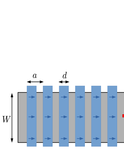
Figure 6: Left: top view of a periodic array of magnetic bars perpendicular to the flow direction shown by the red arrow. The period of the array is $a$ and the width of the bar is $d$. The bars are magnetized parallel to the longitudinal axis of the channel. The direction of the magnetization is shown by the blue arrows. Right: Side view of the device. The vertical distance from the bar magnets to the 2DEG is $z$ and the thickness of the rectangular bar is $\delta z$.

The bars are magnetized along the longitudinal axis of the channel. The bar thickness is $\delta z$ and the distance from the base of the bar to the 2DEG is $z$, shown in the right panel of Fig. 6. We set the value of the period $a=2.6\mu$m as obtained in Sec. II. We tune the remaining free parameters $d,z,\delta z$ such that the z-component of magnetic field in the 2DEG is approximately $B_{0}\sin(2\pi x/a)$ with $B_{0}\approx 30$ mT. This value of $B_{0}$ limits the magnetic correction to the viscosity to a maximum of approximately 2% and thus this effect may be safely neglected in the analysis. Assuming the magnetic moment is uniform throughout the volume of each bar, and the bars extend in the transverse ($y$) direction wider than the width $W$ of the sample, we calculate the magnetic field on the plane of 2DEG as a function of longitudinal coordinate $x$, from the Biot-Savart law as

$$\frac{B_{z}(x)}{B_{m}}\bigg{|}_{2DEG}=-\sum_{n>1}\frac{\sin\left(gnd/2\right)}{\pi n}\sin(gnx)Z_{n},\\ Z_{n}(z,\delta z)=e^{-gnz}(1-e^{-gn\delta z}),$$ (21)

where $B_{m}$ is the saturation field, and $x$ is measured from the center of one of the magnets. For example, at the edge of the magnet $x=d/2$, the harmonics of the field on 2DEG plane is $\propto\sin^{2}(gnd/2)$. Therefore, $d=a/2=\pi/g$ maximizes the first harmonic and suppresses the second harmonic. We numerically calculate $B$ from Eq (21) and further confirm that $d=a/2=1.3\>\mu$m is optimal. In other words, matching the width of the magnet to the spacing between successive magnets creates an effectively sinusoidal magnetic field profile without higher harmonics.

We consider two magnetic materials, (i) Ni that has saturation magnetic field 600mT [52] and (ii) NiFe alloy that has saturation magnetic field 1500mT. [53] We consider two values of bar thickness, $\delta z=0.3\>\mu$m and $\delta z=0.2\>\mu$m. After fixing these values, the only free parameter is the distance to 2DEG $z$, which we tune.

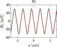
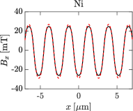
Figure 7: Magnetic field in the 2DEG plane for Ni bars. Left panel: $B_{z}$ versus $x$. Right panel: $B_{x}$ versus $x$. The parameter sets are: black solid line $\delta z=0.2\>\mu\mathrm{m},\ z=0.4\>\mu\mathrm{m}$, red dashed line $\delta z=0.3\>\mu\mathrm{m},\ z=0.5\>\mu\mathrm{m}$.

Plots of $B_{z}$ versus $x$ for Ni bars for $\delta z=0.2\>\mu\mathrm{m},\ z=0.4\>\mu\mathrm{m}$ and for $\delta z=0.3\>\mu\mathrm{m},\ z=0.5\>\mu\mathrm{m}$ are presented in the left panel of Fig. 7. Fields for these parameter sets are practically indistinguishable and close to the simple sinusoidal dependence with amplitude $30$ m T. In the right panel of Fig. 7 we plot the $x$-component of magnetic field for the same sets of parameters. Of course the $x$-component does not influence hydrodynamics, but it remains instructive to see the magnitude and the $x$-dependence.

Plots of $B_{z}$ versus $x$ for NiFe bars for ($\delta z=0.2\>\mu\mathrm{m},\ z=0.75\>\mu\mathrm{m}$) and for ($\delta z=0.3\>\mu\mathrm{m},\ z=0.87\>\mu\mathrm{m}$) are presented in the left panel of Fig. 8. Again, fields for these parameter sets are practically indistinguishable and closely follow a sinusoidal pattern as desired. In the right panel of Fig. 8 we plot the $x$-component of magnetic field for the same sets of parameters.

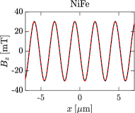
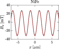
Figure 8: Magnetic field in the 2DEG plane for NiFe bars. Left panel: $B_{z}$ versus $x$. Right panel: $B_{x}$ versus x. The parameter sets are: black solid line $\delta z=0.2\>\mu\mathrm{m},\ z=0.75\>\mu\mathrm{m}$, red dashed line $\delta z=0.3\mu m,\ z=0.87\>\mu\mathrm{m}$.

V Conclusions

In this work we propose a new method to study viscous hydrodynamic flow of electrons in 2D mesoscopic systems. This method involves the use of micromagnets to drive oscillatory flow everywhere in the fluid domain, promoting viscous dissipation not just in the boundary layer but also in the bulk. The proposed method allows for improved precision of hydrodynamic measurements by at least an order of magnitude compared to existing state-of-the-art experiments. With such an improvement in accuracy, electron hydrodynamics presents itself as a novel and efficient method to study electron-electron correlations.

Appendix A Perturbative solution of boundary layer to second order

In Sec. III.1 we presented the perturbative boundary layer solution to first order. This first order solution was derived by solving Eq.(7a) for the stream function, defined in Eq. (II), to first obtain the driven solution and then again for a judiciously crafted free solution. The generalized complete first order solution was then subject to the boundary conditions, Eq.(11), in order to completely define all coefficients. Now, this process can be repeated ad infinitum to obtain higher order corrections of the series

$$\psi=v_{0}y+v_{0}\sum_{n=1}^{\infty}(\omega\tau)^{n}\psi^{(n)}.$$ (22)

Here $\psi^{(n)}$ independently satisfies the boundary conditions Eq. (11) at each order of correction. For simplicity we write distance in units $D=1$. We may decompose $\psi^{(n)}$ into free and driven components as we did to first order in the text

$$\psi^{(n)}=\psi_{f}^{(n)}+\psi_{d}^{(n)},\quad(-\nabla^{2}+\nabla^{4})\psi_{f}^{(n)}=0.$$ (23)

The free solution must be of the form

$$\psi_{f}^{(n)}=\sum_{m=1}^{n}\sum_{s=0,1}A^{(n)}_{m,s}\cos(mgx)e^{-\lambda_{m,s}y},$$ (24)

where

$$\lambda_{m,s}=\sqrt{m^{2}g^{2}+s},\quad s=0,1.$$ (25)

The Stokes operator, $-\nabla^{2}+\nabla^{4}$, becomes invertible when acting on the driven solution. Therefore the driven solution can be written as

$$\psi_{d}^{(n)}=\sum_{\lambda}\sum_{m=1}^{n}B^{(n)}_{m}(\lambda)\cos(mgx)e^{-\lambda y},$$ (26)

where $\lambda$ is chosen from the set of $\lambda_{m^{\prime},s}$ given by the formula in Eq. (25), defined for the indices $0\leq m^{\prime}<n$ and $s=0,1$. We also note that, in this choice, the term with $B_{m}^{(n)}(\lambda_{m,s})$ never appears, as it is part of the homogeneous solution (i.e. it belongs to the kernel of the Stokes operator).

To first order the Stokes equation, Eq. (7a), reads

$$\sum_{\lambda}B^{(1)}_{1}(\lambda)e^{-\lambda y}(\lambda^{2}-\lambda_{1,0}^{2})(\lambda^{2}-\lambda^{2}_{1,1})=g.$$ (27)

This equation is satisfied only for $\lambda=\lambda_{0,0}=0$. Therefore the only non-vanishing coefficient is

$$B^{(1)}_{1}(\lambda_{0,0})=\frac{g}{\lambda_{1,0}^{2}\lambda^{2}_{1,1}}=\frac{1}{g(g^{2}+1)}.$$ (28)

The remaining two coefficients, $A^{(1)}_{1,s}$ where $s=0,1$, may be determined from the boundary conditions, Eq. (11).

$$\sum_{s=0,1}A^{(1)}_{1,s}+B_{1}^{(1)}(\lambda_{0,0}) = 0,$$ (29)

$$\sum_{s=0,1}A^{(1)}_{1,s}\lambda_{1,s}^{2} = 0.$$ (30)

The solutions are $A^{(1)}_{1,s}=-g(-1)^{s}\lambda_{1,s}^{-2}$ where $s=0,1$, or explicitly

$$A_{1,0}^{(1)} = -\frac{g}{\lambda_{1,0}^{2}}=-\frac{1}{g},$$ (31)

$$A_{1,1}^{(1)} = \frac{g}{\lambda_{1,1}^{2}}=\frac{g}{g^{2}+1}.$$ (32)

The first order solution is completely defined by the coefficients $A^{(1)}_{1,0},A^{(1)}_{1,1}$ and $B^{(1)}_{1}(\lambda_{0,0})$, written explicitly as Eq. (III.1) in the main text.

The first order solution, $\psi^{(1)}$, acts as a source for the second order driven solution, $\psi_{d}^{(2)}$. By solving the Stokes equation, Eq. (7a), we find the non-vanishing coefficients of $\psi_{d}^{(2)}$ to be

$$B_{m}^{(2)}(\lambda_{1,s})=\frac{(-1)^{s}g^{2}}{2\lambda_{1,s}(\lambda_{1,s}^{2}-\lambda_{m,0}^{2})(\lambda_{1,s}^{2}-\lambda_{m,1}^{2})},\\ \mathrm{for}\quad m=0,2,\>s=0,1.$$ (33)

To satisfy the boundary conditions, Eq. (11), the second order free solution has non-vanishing coefficients $A^{(2)}_{m,s}$ for $m=0,2$ and $s=0,1$. The coefficient $A^{(2)}_{0,0}$ precedes a constant term and thus its value does not affect the current and voltage distribution. The boundary conditions provide three equations for the remaining three coefficients. Setting $A^{(2)}_{0,0}$ appropriately, we have

$$A_{m,r}^{(2)}=\frac{g^{2}}{2}\sum_{s=0,1}\frac{(-1)^{r+s}}{\lambda_{1,s}(\lambda_{1,s}^{2}-\lambda_{m,r}^{2})},\\ \mathrm{for}\quad m=0,2,\>r=0,1.$$ (34)

Evidently, the leading term of the second order correction decays at a faster rate than that of the first order correction. Higher order boundary layers decay at a rate faster than that of $\exp(-gy)$ or $\exp(-y/D)$. Thus in the perturbative regime, $\omega\tau<1$, the width of the boundary layer is finite with an effective width comparable to the largest of $D$ and $1/g$.

References

- Gurzhi [1968] R. N. Gurzhi, Hydrodynamic effects in solids at low temperature, Soviet Physics Uspekhi 11, 255 (1968), publisher: IOP Publishing.
- Polini and Geim [2020] M. Polini and A. K. Geim, Viscous electron fluids, Physics Today 73, 28 (2020).
- Gurzhi [1963] R. N. Gurzhi, Minimum of Resistance in Impurity-free Conductors, JETP 17, 521 (1963).
- de Jong and Molenkamp [1995] M. J. M. de Jong and L. W. Molenkamp, Hydrodynamic electron flow in high-mobility wires, Phys. Rev. B 51, 13389 (1995), publisher: American Physical Society.
- Lucas and Fong [2018] A. Lucas and K. C. Fong, Hydrodynamics of electrons in graphene, Journal of Physics: Condensed Matter 30, 053001 (2018), publisher: IOP Publishing.
- Gurzhi et al. [1995] R. N. Gurzhi, A. N. Kalinenko, and A. I. Kopeliovich, Electron-Electron Collisions and a New Hydrodynamic Effect in Two-Dimensional Electron Gas, Physical Review Letters 74, 3872 (1995).
- Bandurin et al. [2016] D. A. Bandurin, I. Torre, R. K. Kumar, M. Ben Shalom, A. Tomadin, A. Principi, G. H. Auton, E. Khestanova, K. S. Novoselov, I. V. Grigorieva, L. A. Ponomarenko, A. K. Geim, and M. Polini, Negative local resistance caused by viscous electron backflow in graphene, Science 351, 1055 (2016), publisher: American Association for the Advancement of Science.
- Moll et al. [2016] P. J. W. Moll, P. Kushwaha, N. Nandi, B. Schmidt, and A. P. Mackenzie, Evidence for hydrodynamic electron flow in $\mathrmPdCoO_2$, Science 351, 1061 (2016), publisher: American Association for the Advancement of Science.
- Alekseev [2016] P. S. Alekseev, Negative Magnetoresistance in Viscous Flow of Two-Dimensional Electrons, Phys. Rev. Lett. 117, 166601 (2016), publisher: American Physical Society.
- Krishna Kumar et al. [2017] R. Krishna Kumar, D. A. Bandurin, F. M. D. Pellegrino, Y. Cao, A. Principi, H. Guo, G. H. Auton, M. Ben Shalom, L. A. Ponomarenko, G. Falkovich, K. Watanabe, T. Taniguchi, I. V. Grigorieva, L. S. Levitov, M. Polini, and A. K. Geim, Superballistic flow of viscous electron fluid through graphene constrictions, Nature Physics 13, 1182 (2017), iSBN: 1745-2481.
- Bandurin et al. [2018] D. A. Bandurin, A. V. Shytov, L. S. Levitov, R. K. Kumar, A. I. Berdyugin, M. Ben Shalom, I. V. Grigorieva, A. K. Geim, and G. Falkovich, Fluidity onset in graphene, Nature Communications 9, 4533 (2018).
- Keser et al. [2021] A. C. Keser, D. Q. Wang, O. Klochan, D. Y. H. Ho, O. A. Tkachenko, V. A. Tkachenko, D. Culcer, S. Adam, I. Farrer, D. A. Ritchie, O. P. Sushkov, and A. R. Hamilton, Geometric control of universal hydrodynamic flow in a two-dimensional electron fluid, Phys. Rev. X 11, 031030 (2021).
- Gusev et al. [2018a] G. M. Gusev, A. D. Levin, E. V. Levinson, and A. K. Bakarov, Viscous transport and Hall viscosity in a two-dimensional electron system, Phys. Rev. B 98, 161303(R) (2018a), publisher: American Physical Society.
- Ginzburg et al. [2021] L. V. Ginzburg, C. Gold, M. P. Röösli, C. Reichl, M. Berl, W. Wegscheider, T. Ihn, and K. Ensslin, Superballistic electron flow through a point contact in a Ga[Al]As heterostructure, Physical Review Research 3, 023033 (2021), arXiv: 2012.03570.
- Sulpizio et al. [2019] J. A. Sulpizio, L. Ella, A. Rozen, J. Birkbeck, D. J. Perello, D. Dutta, M. Ben-Shalom, T. Taniguchi, K. Watanabe, T. Holder, R. Queiroz, A. Principi, A. Stern, T. Scaffidi, A. K. Geim, and S. Ilani, Visualizing Poiseuille flow of hydrodynamic electrons, Nature 576, 75 (2019), iSBN: 1476-4687.
- Ku et al. [2020] M. J. H. Ku, T. X. Zhou, Q. Li, Y. J. Shin, J. K. Shi, C. Burch, L. E. Anderson, A. T. Pierce, Y. Xie, A. Hamo, U. Vool, H. Zhang, F. Casola, T. Taniguchi, K. Watanabe, M. M. Fogler, P. Kim, A. Yacoby, and R. L. Walsworth, Imaging viscous flow of the Dirac fluid in graphene, Nature 583, 537 (2020), iSBN: 1476-4687.
- Ella et al. [2019] L. Ella, A. Rozen, J. Birkbeck, M. Ben-Shalom, D. Perello, J. Zultak, T. Taniguchi, K. Watanabe, A. K. Geim, S. Ilani, and J. A. Sulpizio, Simultaneous voltage and current density imaging of flowing electrons in two dimensions, Nature Nanotechnology 14, 480 (2019), number: 5 Publisher: Nature Publishing Group.
- Govorov and Heremans [2004] A. O. Govorov and J. J. Heremans, Hydrodynamic Effects in Interacting Fermi Electron Jets, Phys. Rev. Lett. 92, 026803 (2004), publisher: American Physical Society.
- Kaya [2013] I. I. Kaya, Nonequilibrium transport and the bernoulli effect of electrons in a two-dimensional electron gas, Modern Physics Letters B 27, 1330001 (2013), _eprint: https://doi.org/10.1142/S0217984913300019.
- Braem et al. [2018] B. A. Braem, F. M. D. Pellegrino, A. Principi, M. Röösli, C. Gold, S. Hennel, J. V. Koski, M. Berl, W. Dietsche, W. Wegscheider, M. Polini, T. Ihn, and K. Ensslin, Scanning gate microscopy in a viscous electron fluid, Physical Review B 98, 241304 (2018), publisher: American Physical Society.
- Berdyugin et al. [2019] A. I. Berdyugin, S. G. Xu, F. M. D. Pellegrino, R. Krishna Kumar, A. Principi, I. Torre, M. Ben Shalom, T. Taniguchi, K. Watanabe, I. V. Grigorieva, M. Polini, A. K. Geim, and D. A. Bandurin, Measuring Hall viscosity of graphene’s electron fluid, Science 364, 162 (2019), publisher: American Association for the Advancement of Science.
- Gusev et al. [2018b] G. M. Gusev, A. D. Levin, E. V. Levinson, and A. K. Bakarov, Viscous electron flow in mesoscopic two-dimensional electron gas, AIP Advances 8, 025318 (2018b).
- Shi et al. [2014] Q. Shi, P. D. Martin, Q. A. Ebner, M. A. Zudov, L. N. Pfeiffer, and K. W. West, Colossal negative magnetoresistance in a two-dimensional electron gas, Phys. Rev. B 89, 201301(R) (2014), publisher: American Physical Society.
- Mani et al. [2013] R. G. Mani, A. Kriisa, and W. Wegscheider, Size-dependent giant-magnetoresistance in millimeter scale GaAs/AlGaAs 2D electron devices, Scientific Reports 3, 2747 EP (2013), publisher: The Author(s) SN -.
- Wang et al. [2022] X. Wang, P. Jia, R.-R. Du, L. N. Pfeiffer, K. W. Baldwin, and K. W. West, Hydrodynamic charge transport in gaas/algaas ultrahigh-mobility two-dimensional electron gas (2022).
- Crossno et al. [2016] J. Crossno, J. K. Shi, K. Wang, X. Liu, A. Harzheim, A. Lucas, S. Sachdev, P. Kim, T. Taniguchi, K. Watanabe, T. A. Ohki, and K. C. Fong, Observation of the Dirac fluid and the breakdown of the Wiedemann-Franz law in graphene, Science 351, 1058 (2016).
- Gooth et al. [2018] J. Gooth, F. Menges, N. Kumar, V. Süss, C. Shekhar, Y. Sun, U. Drechsler, R. Zierold, C. Felser, and B. Gotsmann, Thermal and electrical signatures of a hydrodynamic electron fluid in tungsten diphosphide, Nature Communications 9, 4093 (2018).
- Lucas and Das Sarma [2018] A. Lucas and S. Das Sarma, Electronic hydrodynamics and the breakdown of the wiedemann-franz and mott laws in interacting metals, Phys. Rev. B 97, 245128 (2018).
- Jaoui et al. [2021] A. Jaoui, B. Fauqué, and K. Behnia, Thermal resistivity and hydrodynamics of the degenerate electron fluid in antimony, Nature Communications 12, 195 (2021), number: 1 Publisher: Nature Publishing Group.
- Ahn and Das Sarma [2022] S. Ahn and S. Das Sarma, Hydrodynamics, viscous electron fluid, and wiedeman-franz law in two-dimensional semiconductors, Phys. Rev. B 106, L081303 (2022).
- Dai et al. [2010] Y. Dai, R. R. Du, L. N. Pfeiffer, and K. W. West, Observation of a cyclotron harmonic spike in microwave-induced resistances in ultraclean quantum wells, Phys. Rev. Lett. 105, 246802 (2010).
- Hatke et al. [2011] A. T. Hatke, M. A. Zudov, L. N. Pfeiffer, and K. W. West, Giant microwave photoresistivity in high-mobility quantum hall systems, Phys. Rev. B 83, 121301 (2011).
- Białek et al. [2015] M. Białek, J. Łusakowski, M. Czapkiewicz, J. Wróbel, and V. Umansky, Photoresponse of a two-dimensional electron gas at the second harmonic of the cyclotron resonance, Phys. Rev. B 91, 045437 (2015).
- Alekseev and Alekseeva [2019] P. S. Alekseev and A. P. Alekseeva, Transverse magnetosonic waves and viscoelastic resonance in a two-dimensional highly viscous electron fluid, Phys. Rev. Lett. 123, 236801 (2019).
- Gallagher et al. [2019] P. Gallagher, C.-S. Yang, T. Lyu, F. Tian, R. Kou, H. Zhang, K. Watanabe, T. Taniguchi, and F. Wang, Quantum-critical conductivity of the Dirac fluid in graphene, Science 364, 158 (2019), publisher: American Association for the Advancement of Science.
- Stern et al. [2021] A. Stern, T. Scaffidi, O. Reuven, C. Kumar, J. Birkbeck, and S. Ilani, Spread and erase – How electron hydrodynamics can eliminate the Landauer-Sharvin resistance, arXiv:2110.15369 [cond-mat] (2021), arXiv: 2110.15369.
- Varnavides et al. [2020] G. Varnavides, A. S. Jermyn, P. Anikeeva, C. Felser, and P. Narang, Electron hydrodynamics in anisotropic materials, Nature Communications 11, 4710 (2020), number: 1 Publisher: Nature Publishing Group.
- Link et al. [2018] J. M. Link, B. N. Narozhny, E. I. Kiselev, and J. Schmalian, Out-of-Bounds Hydrodynamics in Anisotropic Dirac Fluids, Phys. Rev. Lett. 120, 196801 (2018), publisher: American Physical Society.
- Galitski et al. [2018] V. Galitski, M. Kargarian, and S. Syzranov, Dynamo Effect and Turbulence in Hydrodynamic Weyl Metals, Phys. Rev. Lett. 121, 176603 (2018), publisher: American Physical Society.
- Tatara [2021] G. Tatara, Hydrodynamic theory of vorticity-induced spin transport, Physical Review B 104, 184414 (2021), publisher: American Physical Society.
- Doornenbal et al. [2019] R. J. Doornenbal, M. Polini, and R. A. Duine, Spin–vorticity coupling in viscous electron fluids, Journal of Physics: Materials 2, 015006 (2019), publisher: IOP Publishing.
- Matsuo et al. [2020] M. Matsuo, D. A. Bandurin, Y. Ohnuma, Y. Tsutsumi, and S. Maekawa, Spin hydrodynamic generation in graphene, arXiv:2005.01493 [cond-mat] (2020), arXiv: 2005.01493 version: 1.
- Takahashi et al. [2016] R. Takahashi, M. Matsuo, M. Ono, K. Harii, H. Chudo, S. Okayasu, J. Ieda, S. Takahashi, S. Maekawa, and E. Saitoh, Spin hydrodynamic generation, Nature Physics 12, 52 (2016), number: 1 Publisher: Nature Publishing Group.
- Takahashi et al. [2020] R. Takahashi, H. Chudo, M. Matsuo, K. Harii, Y. Ohnuma, S. Maekawa, and E. Saitoh, Giant spin hydrodynamic generation in laminar flow, Nature Communications 11, 3009 (2020), number: 1 Publisher: Nature Publishing Group.
- Landau and Lifshitz [2013] L. Landau and E. Lifshitz, Fluid Mechanics, Vol. 6 (Elsevier Science, 2013).
- Alekseev and Dmitriev [2020] P. S. Alekseev and A. P. Dmitriev, Viscosity of two-dimensional electrons, Physical Review B 102, 241409 (2020).
- Moessner et al. [2018] R. Moessner, P. Surówka, and P. Witkowski, Pulsating flow and boundary layers in viscous electronic hydrodynamics, Physical Review B 97, 161112 (2018), arXiv: 1710.00354.
- Levchenko and Schmalian [2020] A. Levchenko and J. Schmalian, Transport properties of strongly coupled electron–phonon liquids, Annals of Physics 419, 168218 (2020).
- Gusev et al. [2020] G. M. Gusev, A. S. Jaroshevich, A. D. Levin, Z. D. Kvon, and A. K. Bakarov, Stokes flow around an obstacle in viscous two-dimensional electron liquid, Scientific Reports 10, 7860 (2020), iSBN: 2045-2322.
- Lucas [2017] A. Lucas, Stokes paradox in electronic Fermi liquids, Phys. Rev. B 95, 115425 (2017), publisher: American Physical Society.
- Moessner et al. [2019] R. Moessner, N. Morales-Durán, P. Surówka, and P. Witkowski, Boundary condition and geometry engineering in electronic hydrodynamics, Physical Review B 100, 155115 (2019), arXiv: 1903.08037.
- Danan et al. [1968] H. Danan, A. Herr, and A. J. P. Meyer, New Determinations of the Saturation Magnetization of Nickel and Iron, Journal of Applied Physics 39, 669 (1968).
- Tumanski [2011] S. Tumanski, Magnetic Materials, in Handbook of Magnetic Measurements, Vol. 20110781 (CRC Press, 2011) pp. 117–158, series Title: Series in Sensors.