Hopf Bifurcation in vibrational resonance through modulation of fast frequency

Abstract

In this Letter we explore the possibility of a supercritical Hopf bifurcation in a typical parametric nonlinear oscillator which has been excited by two frequencies, one slow and the other fast, through the variation of the frequency of the rapidly oscillating driving force. Studies of nonlinear responses and bifurcations of such driven nonlinear systems are usually done by treating the strength of the fast drive as the control parameter. Here we show that, beyond its role in allowing one to study the dynamics with the slow and fast components nicely separated, the fast frequency can also be used as an independent control parameter for studying Hopf bifurcation.

Keywords: Vibrational resonance, Parametric Oscillator, van der Pol-Mathieu-Duffing oscillator, Bistability, Hopf Bifurcation

Corresponding author (email):
roysomnath63@gmail.com

I Introduction

The subject of Vibrational Resonance has burgeoned to a significant volume of literature in nonlinear dynamics over the past two decades. The response of nonlinear systems to two separate driving forces one with slower frequency and the other with a frequency much faster than the former one, has been the standard paradigm for all models proposed and studied within the ambit of vibrational resonance McClintock ; gitterman ; bleckhamn ; Baltanas ; Chizhevsky ; Knoll ; Jeyakumari ; Rajasekar ; Jeevarathinam ; Jeyakumari1 ; Ullner ; Yang ; Daza ; Zaikin ; ddas ; Shyamolina . In a recent study we have explored the effect of vibrational resonance for a certain parametric oscillator which in the literature has been named Van der Pol-Mathieu-Duffing oscillator. There are two basic motivations behind our studying this oscillator. Firstly, as there is already a parametric frequency associated with the oscillator in addition to its own natural frequency, study of vibrational resonance for such an oscillator is usually done by bringing in a single forcing term with very high frequency belhaq ; belhaq1 ; belhaq2 ; belhaq3 ; PSDR . Studies pertaining to the response of such systems in presence of an additional forcing term with frequency much slower than the fast drive has therefore been rare. Secondly, due to the spatially nonlinear nature of the damping of a self-excited oscillator, it turns out that the action of these twin forcing terms results in a modification of the damping along with the natural frequency of the oscillator. While the latter phenomenon, where the natural frequency of the system gets modified in the slow dynamics of the oscillator, is a widely addressed issue in the context of vibrational resonance, the former phenomenon, where the damping undergoes a modification, is relatively less explored. It is precisely this phenomenon that gives a supercritical Hopf bifurcation in the oscillator under study. But, the interesting aspect that transpires is, this bifurcation can be effected in two ways: one, by varying the strength of the fast driving term while keeping the frequency constant, and two, by varying the fast frequency itself while keeping the strength constant. The first procedure is more in keeping with traditional studies of systems showing vibrational resonance and has been studied in detail in a recent communication sroy2 . The second procedure is the subject of this Letter, which, to the best of our knowledge, has not been much investigated earlier.

THE MODEL AND FLOW EQUATIONS

The model oscillator that we are studying here is given by the following equation:

$$\ddot{x}+\gamma(x^{2}-1)\dot{x}-\omega_{0}^{2}(1+h\cos\omega_{p}t)x+\alpha x^{3}=c\cos\omega t+g\cos\Omega t$$ (1)

where $\omega_{0}$ is the natural frequency of the oscillator. The parametric excitation is done through the term $h\cos\omega_{p}t$ where the magnitude of the parametric frequency will be chosen to be $\omega_{p}=2\omega_{0}$ sroy2 . On the right hand side of the above equation, there are two driving terms, $c\cos\omega t$ and $g\cos\Omega t$, with the frequency of the latter term much greater than that of the former, viz., $\Omega>>\omega$. When the parameter $h$, the strength of the parametric drive, falls in the range $-1<h<1$ we have a bistable oscillator in unstable equilibrium on the crest of a double well. The effect of the high frequency drive $g\cos\Omega t$ is to redress this bistability to an effective monostable potential where the system oscillates about a stable equilibrium.

This effective slow dynamics can be derived by first separating the dynamical variable $x$ into a slow variable $s$ and a fast variable $f$

$$x(t)=s(t,\omega t)+f(t,\Omega t).$$ (2)

The fastness of the variable $f$ gets reflected in the fact that the averages of the odd moments over a complete time period are zero, viz., $\langle f\rangle=\langle f^{3}\rangle=0$ while the value of $\langle f^{2}\rangle$, after some algebra sroy2 evaluates to $\langle f^{2}\rangle=Mg^{2}/2$, where $M=1/\kappa^{2}$ with $\kappa$ given as

$$\kappa=\frac{\Omega^{2}(\Omega^{2}+\gamma^{2})}{\sqrt{(\Omega^{2}-\omega_{0}^{2})^{2}+\Omega^{2}\gamma^{2}}}=\frac{1}{\sqrt{M}}$$ (3)

Eventually, all the average effects of the fast variable get incorporated into the equation of the slow variable thus leading to an effective equation for the slow variable as

$$\ddot{s}+\gamma(s^{2}+K)\dot{s}+({\tilde{\omega}}^{2}-\omega_{0}^{2}h\cos\omega_{p}t)s+\alpha s^{3}=c\cos\omega t$$ (4)

where the frequency term $\tilde{\omega}$ is given by

$$\tilde{\omega}^{2}(g,\Omega) = 3\alpha\left\langle f^{2}\right\rangle-\omega_{0}^{2}$$ (5)

$$= \frac{3}{2}\alpha g^{2}M-\omega_{0}^{2}$$

and the factor associated with the nonlinear damping $K$ takes the form

$$K(g,\Omega)=\frac{g^{2}}{2}M(\Omega)-1.$$ (6)

Defining an effective frequency as $\omega_{eff}=\sqrt{{\tilde{\omega}}^{2}-\omega_{0}^{2}h\cos\omega_{p}t}$ we can identify an effective monostable potential $V_{mono}(s,t)=\frac{1}{2}\omega_{eff}^{2}(t)s^{2}+\frac{1}{4}\alpha s^{4}$. The central fact that merits close observation is that the coefficient of $x$ on the left hand side of Eq.(1) is negative, while the coefficient of $s$ on the left hand side of Eq.(4) is positive, provided that, along with the previously imposed condition on $h$ (viz. $-1<h<+1$), we have an additional condition $-{\tilde{\omega}}^{2}<\omega_{0}^{2}h<{\tilde{\omega}}^{2}$.

In Eqs.(5) and (6) we have expressed the effective terms $\tilde{\omega}$ and $K$ as functions of the strength $g$ as well as the high frequency $\Omega$ of the fast driving force $g\cos\Omega t$. This opens up the scope for studying the consequence of exciting the system with a slow as well as a fast drive in terms of variation not only of $g$ but also of $\Omega$. The effect of the fast drive term is twofold. Firstly, from Eqs.(4) and (5) we see that the new frequency $\tilde{\omega}$ emerges as an effective natural frequency replacing $\omega_{0}$ of Eq.(1). Secondly, the Van der Pol damping term gets modified from $\gamma(x^{2}-1)\dot{x}$ in Eq.(1) to $\gamma(s^{2}+K)\dot{s}$ in Eq.(4). The question of a Hopf bifurcation arises when this effective damping parameter $K$ passes through a zero in course of its variation with respect to either $g$ or $M$. The effect of the variation in $g$ leading to a Hopf bifurcation has been studied in sroy2 . Here we are exploring the effect of variation of $K$ as a consequence of variation in $M$. From the structure of $M$ given in Eq.(3) it is clear that for large values of $\Omega$ we have $M\sim\Omega^{-4}$, a crucial point to which we shall come a little later.

To make further progress we need to derive the amplitude and phase flow equations from Eq.(4) with the parametric frequency replaced by a value that is twice the value of the slow driving frequency sroy2 , i.e., $\omega_{p}=2\omega$. The flow equations can be arrived at through some standard perturbation technique, for example, multiple-time-scale analysis the details of which have been described in sroy2 . Defining the dimensionless time $\tau=\omega t$, we do the perturbation around the redressed natural frequency $\tilde{\omega}$ by making the frequency $\omega$ of the slow forcing drive perturbatively close to $\tilde{\omega}$ through the introduction of a detuning $\tilde{\sigma}$ as $\omega=\tilde{\omega}+\epsilon\tilde{\sigma}$, where $\epsilon$ is the perturbation parameter denoting smallness. Introducing the rescaled parameters $\Gamma=\gamma/\omega$, $\Lambda=\alpha/{\omega}^{2}$, $C=c/{\omega}^{2}$ and $H=h{\omega_{0}}^{2}/{\omega}^{2}$, we can rearrange Eq.(4) as

$$s^{\prime\prime}+s=\epsilon[-\Gamma(s^{2}+K)s^{\prime}+H(\cos 2\tau)s-\Lambda s^{3}+C\cos\omega\tau+\sigma s]$$ (7)

where the rescaled detuning parameter is defined to first order in $\epsilon$ as ${\tilde{\omega}}^{2}=\omega^{2}(1-\epsilon\sigma)$ with $\sigma=2\tilde{\sigma}\tilde{\omega}/\omega^{2}$. For using multiple-time-scale analysis we can write the perturbation expansion $s(\tau_{0},\tau_{1})=s_{0}(\tau_{0},\tau_{1})+\epsilon(\tau_{0},\tau_{1})+\mathcal{O}(\epsilon^{2})$ and proceeding as usual sroy2 we arrive at the amplitude and phase flow equations

$$\frac{da}{d\tau} = -\frac{1}{2}\Bigg{[}\frac{\Gamma a^{3}}{4}+\Gamma Ka+C\sin\theta+\frac{Ha}{2}\sin(2\theta)\Bigg{]}$$

(8)

$$\frac{d\theta}{d\tau} = \frac{1}{2}\Bigg{[}\frac{3\Lambda}{4}a^{2}-\sigma-\frac{C}{a}\cos\theta-\frac{H}{2}\cos(2\theta)\Bigg{]}$$ (9)

The fixed points of these equations obtained by putting the derivatives equal to zero lead us to those specific locations in the parameter space where we can get the nonlinear responses of the system depicted by peaks in the amplitude curve. By parameter space we mean that we can either study the peaks by varying the strength of the fast frequency drive, $g$, and keeping the other parameter, viz., the high frequency $\Omega$ fixed, or we can go the other way round and obtain peaks by varying $\Omega$ and keeping $g$ fixed. For more specific details in these lines the interested reader is referred to sroy2 ; zhan . We can also use these flow equations to investigate the possibility of creation or destruction of limit cycle through some Hopf bifurcation as one varies either of the parameters $g$ or $\Omega$. For studying the Hopf bifurcation as a result of the variation in the strength $g$, the reader is again referred to sroy2 . In the following we shall study the possibility of Hopf bifurcation as we vary the fast frequency $\Omega$. To the best of our knowledge, this particular investigation has not been done earlier.

HOPF BIFURCATION AND FORMATION OF LIMIT CYCLE

The question of a limit cycle arises because in the initial equation of motion Eq.(1) the expression associated with the damping constant $\gamma$ imparts on the oscillator the capability to self-excite itself. This signature of a Van der Pol damping term leads to a limit cycle through a supercritical Hopf bifurcation. To understand the Hopf bifurcation in the VMD oscillator we are studying here, we have to invoke perturbation theory once again on the flow equations (8) and (9) by introducing a new perturbation parameter $\lambda$ so that the system goes over to a limit cycle over a much longer time-scale given by $t\sim\mathcal{O}(1/\lambda\epsilon)$. This process will lead us to a new set of flow equations which, in the literature, go by the name “super-slow flow” equations strogatz . From these flow equations, we can predict with reasonable accuracy, the point in $\Omega$-space where the origin gets destabilized thus giving birth to a stable limit cycle through a supercritical Hopf bifurcation.

The method of multiple-time scale analysis can be best implemented on the flow equations (8) and (9) through the pair of substitutions $u=a\cos\theta$ and $v=-a\sin\theta$ leading to the following pair of transformed equations:

$$\frac{du}{d\tau} = (-\frac{\sigma}{2}+\frac{H}{4})v+\lambda\bigg{\{}\frac{1}{8}(3\Lambda v-\Gamma u)(u^{2}+v^{2})$$ (10)

$$- \frac{\Gamma Ku}{2}\bigg{\}}$$

$$\frac{dv}{d\tau} = (\frac{\sigma}{2}+\frac{H}{4})u+\lambda\bigg{\{}\frac{c}{2}-\frac{1}{8}(3\Lambda u+\Gamma v)(u^{2}+v^{2})$$ (11)

$$- \frac{\Gamma Kv}{2}\bigg{\}}$$

The arrangement of terms in the above two equations has been made such as to guarantee that at the zeroth order both the variables $u$ and $v$ oscillate simple harmonically with the frequency $\omega_{l}=\sqrt{\frac{\sigma^{2}}{4}-\frac{H^{2}}{16}}$. This is a basic requirement because, the perturbation theory that follows is constructed on the basis of these stable oscillations at the zeroth order. Now, with the different time-scales defined as $T_{j}=\lambda^{j}\tau$, one can write down the perturbation expansions belhaq3 ; rand3 in the parameter $\lambda$ as,

$$u(T_{0},T_{1}) = u_{0}(T_{0},T_{1})+\lambda u_{1}(T_{0},T_{1})+\mathcal{O}(\lambda^{2})$$

$$v(T_{0},T_{1}) = v_{0}(T_{0},T_{1})+\lambda v_{1}(T_{0},T_{1})+\mathcal{O}(\lambda^{2})$$

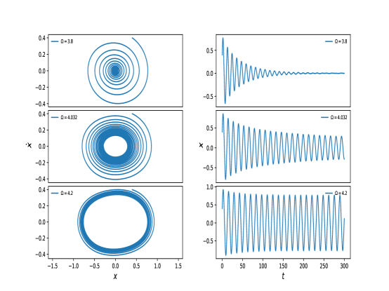
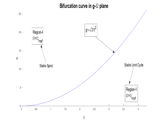
Figure 1: Numerical plot of (7) for supercritical hopf bifurcation: for $g=23,\Omega_{hopf}=4.032$. Other parameters are fixed at $\gamma=0.15,\alpha=0.1,c=0.0005,\omega=\omega_{0}=0.3$ and $h=0.01$.

Figure 2: Bifurcation curve in $g-\Omega$ plane.Region $I$ indicates the zone of stable nodes and region $II$ implicates the zone of stable limit cycles.

By iterating these expansions in Eqs.(10) and (11) order by order, one can proceed with a standard multiple-time scale analysis sroy2 . The zeroth order solutions evaluate to

$$u_{0} = r(T_{1})\cos(\omega_{l}T_{0}+\psi(T_{1}))$$ (13)

$$v_{0} = \frac{\omega_{l}}{p}r(T_{1})\sin(\omega_{l}T_{0}+\psi(T_{1}))$$ (14)

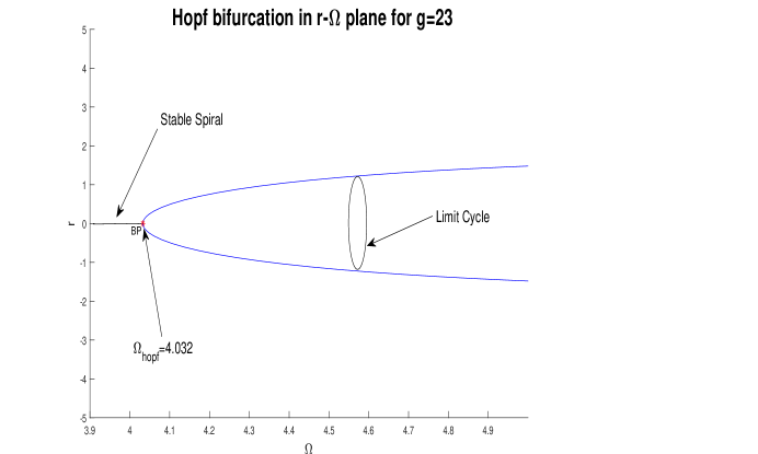
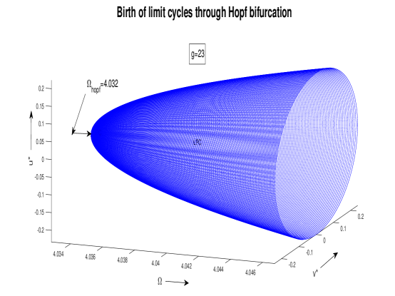
Figure 3: Bifurcation curve in $r-\Omega$ plane for $g=23$ from Eq.(15). All the other parameters are fixed at $\gamma=0.0015,\alpha=0.001,\sigma=0.1,h=0.01$. Hopf point is found at $\Omega_{hopf}=4.032$.

Figure 4: Birth of limit cycle at hopf point(3D perspective) is numerically plotted from Eqs.(10 and 11).Rest of the parameters are fixed at $\gamma=0.0015,\alpha=0.001,\sigma=0.1,h=0.01$. Hopf point is found at $\Omega_{hopf}=4.032$.

where $p=-(\frac{\sigma}{2}-\frac{H}{4})$. Invoking Eqs.(13) and (14) into the first order equations and equating the resonant terms to zero we get the sought after set of (“super-slow”) flow equations as

$$D_{1}r = \frac{-\Gamma K}{2}r-\frac{\sigma\Gamma}{8\sigma-4H}r^{3}$$ (15)

$$D_{1}\psi = -\frac{9\Lambda\sigma^{2}}{4(2\sigma-H)\sqrt{(4\sigma^{2}-H^{2})}}r^{2}.$$ (16)

The two fixed points of the amplitude equation Eq.(15), one being at the origin $r=0$, and the other being at

$$r=\sqrt{K\left(\frac{2H}{\sigma}-4\right)}$$ (17)

gives us the location of a limit cycle, provided the square-root is real. As we have seen above that for stable oscillations at the zeroth order ($u_{0}$ and $v_{0}$) with frequency $\omega_{l}=\sqrt{\frac{\sigma^{2}}{4}-\frac{H^{2}}{16}}$, we must have $H<2\sigma$. This implies that in Eq.(17), $K$ must be negative for a stable limit cycle to form. Looking back at Eq.(15) we see that $K<0$ is indeed the requirement for the origin to be unstable in which case it is only this stable limit cycle where the system can go and settle on. When $K$ is positive, on the other hand, we see that there is no limit cycle anywhere, i.e., no real root for $r$ in Eq.(17), and the system collapses on to a stable origin ($r=0$). Therefore right at $K=0$ a stable limit cycle is born through a Hopf bifurcation in the $K$ parameter space. Furthermore, with $H<2\sigma$, where stable oscillations occur at zeroth order, and on the basis of which this perturbation theory has been built up, we have the coefficient of $r^{3}$ on the right hand side of Eq.(15) as negative thus clearly signalling that the Hopf bifurcation that occurs at $K=0$ is of the supercritical type.

The specific observation, one that has been alluded to heretofore and we intend to propose through this Letter is that, this continuous variation of $K$ through the Hopf point can be achieved in two ways, either by fixing the fast frequency $\Omega$ and varying the strength of the fast drive $g$, or by fixing $g$ and varying the fast frequency $\Omega$ as is clear from the expression for $K\equiv K(g,\Omega)$ appearing in Eq.(6). For $K=0$, the Hopf point, we have therefore the relation

$$M_{hopf}=\frac{2}{[g_{hopf}]^{2}}.$$ (18)

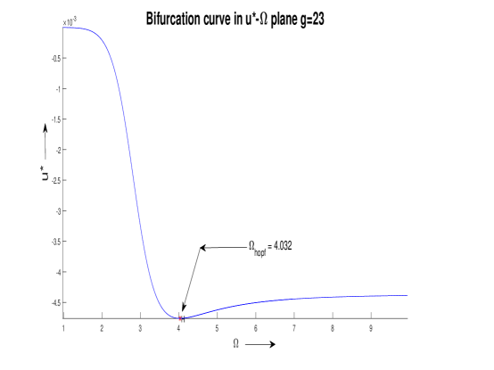
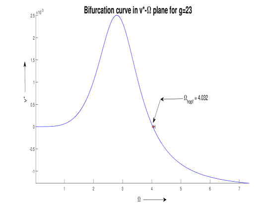
Figure 5: Dynamics of fixed point $u^{*}$ is perceived numerically from Eq.(11 as we increase $\Omega$ .Location of hopf point is denoted by arrow for a fixed g(=23) in $u^{*}-\Omega$ plane.

Figure 6: Dynamics of fixed point $v^{*}$ is perceived numerically from Eq.(10) as we increase $\Omega$ .Location of hopf point is denoted by arrow for a fixed g(=23) in $v^{*}-\Omega$ plane.

If one plots (not done here) $M_{hopf}$ along the $y$-axis and $g_{hopf}$ along the $x$-axis, then one may be misled to think that Eq.(18) is valid through the entire first quadrant of this $g_{hopf}-M_{hopf}$ plane. That this is not the case should be clear from the fact that this entire calculation is based on the fundamental requirement that $\Omega$ is much larger in comparison to $\gamma$ and $\omega_{0}$, and hence from Eq.(3) we get $M\sim\Omega^{-4}$. Accordingly, from Eq.(18) we get that $g_{hopf}\sim\sqrt{2}\Omega_{hopf}^{2}$. For large values of $\Omega$ therefore, we get the region of validity of Eq.(18) as the tail part of the flattening $g_{hopf}-M_{hopf}$ curve, where the values of $g_{hopf}$ are large while the values of $M_{hopf}$ are small. This confirms our observation that apart from $g$, the parameter $\Omega$ can also play the role of a bifurcation parameter. In studies of bifurcations in context of systems showing vibrational resonance, the role of $\Omega$ has been rather confined to being a parameter of much larger value that aids in separating the fast and slow dynamics only. But here we see that along the tail part of the $g_{hopf}-M_{hopf}$ curve, owing to the relation $M\sim\Omega^{-4}$, there is a much smaller change in $M$ corresponding to a much larger change in $\Omega$, and hence, one can scan through a significantly long window of $\Omega$ values to study a situation where apart from $g$, the high frequency $\Omega$ can cause Hopf bifurcations.

NUMERICAL RESULTS

To validate the above analytical results, we have carried out numerical simulations which show quite satisfactory coincide with our study. In (FIG.2), it has been displayed that how the change in parameter $\Omega$ can destabilize a stable node to give birth of a limit cycle through hopf bifurcation. For a fixed value of $g=23$ we numerically plot the phase diagram by simulating the original slow flow Eq.(7), which shows at $\Omega_{hopf}=4.032$ there is a change in stability through hopf bifurcation. This result is in perfect match with our analytical prediction $g_{hopf}\sim\sqrt{2}\Omega_{hopf}^{2}$ which is also verified by conducting numerics on Eq.(10 and 11), delineated in (FIG.2). We have indicated two separate region in this parameter plane $g-\Omega$ region $I$ and $II$. When a particular value of $g$ is fixed, one can have stable nodes in region $I$ where $\Omega<\Omega_{hopf}$. On the other hand, by crossing the hopf line, $g_{hopf}\sim\sqrt{2}\Omega_{hopf}^{2}$ when we arrive at region $II$ where the condition $\Omega>\Omega_{hopf}$ is satisfied, one can think about the existence of limit cycles. Finally, in (FIG.4 and FIG.4) the bifurcation point is pointed out in $r-\Omega$ plane (2D and 3D) by using the Eqs.(15 and 16) which is in fact the implementation of ”super-slow” flow equations Eqs.(10 and 11).We have also portrayed the position of hopf point in the equilibrium plane of $(u^{*},v^{*})$ separately in (FIG.6 and FIG.6).

CONCLUSIONS

To summarize, in this Letter we have explored a new aspect of vibrational resonance in a driven Van der Pol-Mathieu-Duffing oscillator, by showing that apart from treating only the strength of the fast drive as the traditional control parameter to study responses and bifurcations, the fast frequency itself can also be treated as another control parameter. Our main focus here has been to study a supercritical Hopf bifurcation through which the system settles on a stable limit cycle, as result of variation of the fast frequency $\Omega$. We also discuss that owing to very large value of $\Omega$ in comparison to other frequencies and the damping constant, only a specific window of the parameter space can be used for studying this phenomenon. We have come to these conclusions by explicitly deriving flow equations for amplitude and phase for both slow and super-slow dynamics through application of multiple-time-scale perturbation theory. The conclusions thus obtained have also been shown to be reasonably consistent with numerical simulations.

II References

References

- (1) P. Landa, P. McClintock, J. Phys. A 33, L433 (2000)
- (2) M. Gitterman, J.Phys.A 34, L479-L490,(2001)
- (3) I. I. Blechman, Vibrational Mechanics, (World Scientific, Sin- gapore, 2000)
- (4) J. P. Baltanás, L. López, I. I. Blechman, P. S. Landa, A. Zaikin, J. Kurths, M. A. F. Sanjuán, Phys. Rev. E 67, 066119
- (5) V. N. Chizhevsky, E. Smeu, G. Giacomelli, Phys. Rev. Lett. 91, 220602 (2003)
- (6) B. Knoll,F. Keilmann, Nature, volume 399, pages 134–137 (1999)
- (7) S. Jeyakumari, V. Chinnathambi, S. Rajasekar, M. A. F. Sanjuán, Phys. Rev. E 80, 046608 (2009)
- (8) S. Rajasekar, K. Abirami, M. A. F. Sanjuán, Chaos 21, 033106 (2011)
- (9) C. Jeevarathinam, S. Rajasekar, M. A. F. Sanjuán, Phys. Rev. E 83, 066205 (2011)
- (10) S. Jeyakumari, V. Chinnathambi, S. Rajasekar, M. A. F. Sanjuán, Chaos 19, 043128 (2009)
- (11) E. Ullner, A. Zaikin, J. García-Ojalvo, R. Báscones, J. Kurths, Physics Lett.A 312, 348-354 (2003)
- (12) L. Yang, W. Liu, M. Yi, C. Wang, Q. Zhu, X. Zhan, Y. Jia, Phys. Rev. E 86, 016209 (2012)
- (13) A. Daza, A. Wagemakers, S. Rajasekar, M. A. F. Sanjuán, Communications in Nonlinear Science and Numerical Simulation 18, 411-416 (2013)
- (14) A. Zaikin, L. López, J. P. Baltanás, J. Kurths, M. A. F. Sanjuán, Phys. Rev. E 66, 011106 (2002)
- (15) D. Das , D. S. Ray, Eur. Phys. J. B (2018) 91: 279
- (16) S. Ghosh, D. S. Ray, Phys. Rev. E. 88, 042904 (2013)
- (17) M. Belhaq, A. Fahsi, Nonlinear Dyn 53, 139–152 (2008).
- (18) M. Belhaq, S. Sah, Commun. Nonlin. Sci. Numer. Simul. 13, 1706 (2008)
- (19) M. Belhaq, A. Fahsi, Nonlinear Dyn 57, 275–287 (2009).
- (20) M. Belhaq, M. Houssni, Nonlinear Dyn. 18, 1–24 (1999)
- (21) P. Sarkar, S. Paul, D. S. Ray, J. Stat.Mech 2019, 063211 (2019)
- (22) M. Pandey, R. H. Rand, A. Zehnder, Commun. Nonlinear. Sci. Numer. Simul. 12, 1291– 1301 (2007).
- (23) M. Pandey, R. H. Rand, A. Zehnder, Nonlinear Dyn 54, 3–12 (2008).
- (24) R. H. Rand, K. Guennoun, M. Belhaq, Nonlinear Dyn. 31, 187–193 (2003)
- (25) S. Roy, D. Das, D. Banerjee, International Journal of Non-Linear Mechanics, 135, 103771, ISSN 0020-7462, 2021.
- (26) C. Yao, Y. Liu, M. Zhan, Phys. Rev. E., 83, 061122, (2011)
- (27) S. H. Strogatz, Nonlinear Dynamics And Chaos: With Applications To Physics, Biology, Chemistry, And Engineering