Region-Aware Metric Learning for Open World Semantic Segmentation via Meta-Channel Aggregation

Abstract

As one of the most challenging and practical segmentation tasks, open-world semantic segmentation requires the model to segment the anomaly regions in the images and incrementally learn to segment out-of-distribution (OOD) objects, especially under a few-shot condition. The current state-of-the-art (SOTA) method, Deep Metric Learning Network (DMLNet), relies on pixel-level metric learning, with which the identification of similar regions having different semantics is difficult. Therefore, we propose a method called region-aware metric learning (RAML), which first separates the regions of the images and generates region-aware features for further metric learning. RAML improves the integrity of the segmented anomaly regions. Moreover, we propose a novel meta-channel aggregation (MCA) module to further separate anomaly regions, forming high-quality sub-region candidates and thereby improving the model performance for OOD objects. To evaluate the proposed RAML, we have conducted extensive experiments and ablation studies on Lost And Found and Road Anomaly datasets for anomaly segmentation and the CityScapes dataset for incremental few-shot learning. The results show that the proposed RAML achieves SOTA performance in both stages of open world segmentation. Our code and appendix are available at https://github.com/czifan/RAML.

1 Introduction

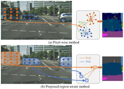
Figure 1: Main idea of our proposed method. (a) Existing methods focus on pixel-level which may result in fine-grained segmentation errors. (b) Our proposed Region-Aware Metric Learning (RAML) method maintains the semantic integrity of the OOD objects.

The breakthrough of deep learning in many fields of computer vision is based on the closed set assumption, which means that all classes in the test should be covered in the training set. However, this assumption rarely holds in the open world. Since most computer vision applications have to deal with unknown classes, models, especially the deep models, must handle the out-of-distribution (OOD) data. Quite a number of work for image recognition and classification in the open world has been proposed since the first introduction of the concept “open world” in Bendale and Boult (2015). However, the work about open world segmentation is scarce. It is not until recently that Cen et al. (2021) proposes a two-step framework to achieve open world semantic segmentation. The framework consists of (1) an anomaly segmentation module that extends the close-set model of in-distribution objects to delineate the unknown regions of the OOD objects correctly, and (2) an incremental few-shot learning module that separates the unknown regions into OOD objects with novel classes. They also introduce metric learning into both stages of open world segmentation, and the results prove that their proposed criteria of metric learning can improve the model’s segmentation of OOD objects.

Although this pilot work provides a good framework for open world segmentation tasks, the model can be improved in two aspects for better performance. First, the metric learning in Cen et al. (2021) relies on the pixel-wise feature embeddings, which may falsely split the object into pieces and result in numerous fine-grained segmentation errors. For example, as shown in Figure 1, the bus wheels and the car wheels have similar feature embeddings and are highly likely to be classified into one group according to the pixel-wise feature embeddings, but they apparently belong to different classes in semantic segmentation. To solve this kind of problems, we propose region-aware metric learning (RAML) for open world segmentation, which significantly outperforms pixel-wise metric learning (PML) in multiple experiments.

Moreover, we improve the model performance, especially for the incremental few-shot learning stage, by introducing a novel region separation module named meta-channel aggregation (MCA). MCA first aims at over-segmenting the unknown regions into several meta channels. Regions belonging to different meta channels are aggregated to form a segmentation of the objects and then evaluated by the Region-aware Metric Learning module.

In addition, Cen et al. (2021) sets a fixed center embedding for each in-distribution class, i.e., a one-hot vector in the feature space. Although the fixed center embedding can effectively create a distance between the distribution of different classes, it ignores the relative similarity between them. For example, in the Cityscapes dataset, the method fails to reveal that the difference between person and rider is smaller than the difference between either of them and sky. This paper aims to overcome the drawback by exploiting a more natural metric learning to constrain the distance between the inter-class region-aware features. Specifically, we replace the one-hot setting in Cen et al. (2021) with Circleloss Sun et al. (2020) as the objective of the metric learning, which not only maintains a fine inter-class distance but also shapes the intra-class distribution more concentrated. Experiments show that such division of the feature space is more conducive to segmenting the OOD data.

In summary, we propose a region-aware metric learning method for open world semantic segmentation. Our contributions are as follows:

• We propose using the region-aware over pixel-wise features for open world semantic segmentation to ensure better semantic integrity of the segmented OOD objects.

• We introduce the MCA module as a novel region separation method that suits incremental few-shot learning.

• We adopt Circleloss Sun et al. (2020) to enlarge the inter-class distance and reduce the intra-class distance of the data samples, improving the performance of the RAML module.

2 Related Work

2.1 Region-aware Semantic Segmentation

The ideas of how to apply regional information to improve semantic segmentation have been discussed by many research groups recently, including two main threads. First, several works have shown that region-aware information has better contextual representation than pixel-level information to achieve pixel labeling Yuan et al. (2020). Secondly, for image segmentation tasks, region-aware information can be better combined with metric or contrastive learning to manipulate the feature space more effectively Wang et al. (2021); Hu et al. (2021). These ideas inspire our paper, but the above works require a sufficient number of training samples to obtain the reasonable region-aware feature representation, while our work is in an open world setting that can only access a few images with unseen class labels. Therefore, we have to design novel region-separation modules (such as MCA) that fit the open world segmentation tasks.

2.2 Anomaly Segmentation

There are two types of approaches for anomaly segmentation, including uncertainty-based methods and generative model-based methods. Uncertainty refers to the level of not belonging to known classes, widely used to determine abnormal states. The baseline of uncertainty-based methods is maximum softmax probability (MSP) reported by Hendrycks and Gimpel (2017). Hendrycks et al. (2019) then improves MSP using maximum logit (MaxLogit) for better performance on large-scale datasets. Other uncertainty-based methods include using Bayesian neural networks Gal and Ghahramani (2016) and maximizing the entropy of OOD objects in the images Chan et al. (2021). On the other hand, generative model-based methods also perform well, including autoencoder (AE) Baur et al. (2018) and GAN-based methods  Xia et al. (2020). However, generative models suffer from unstable training and usually have complex network backbones.

In this work, we follow the idea of MaxLogit and develop our anomaly segmentation based on non-normalized logit.

2.3 Open World Problem

Bendale and Boult (2015) is the first research that gives the formal definition of “open world”, i.e., an open world model must incrementally learn and extend its generality, thereby making the objects with novel classes “known” to itself. Since then, the research on open world problems has increased, including classification Zhong et al. (2021), object detection Joseph et al. (2021), instance segmentation Saito et al. (2021), among others. However, it is not until recently that Cen et al. (2021) proposes the first framework of open world semantic segmentation. Our work follows the settings in Cen et al. (2021) and divides the problem into anomaly segmentation and incremental few-shot learning. However, to ensure semantic integrity and improve the segmentation performance, we use region-aware feature embedding instead of pixel-wise feature extraction in their original method.

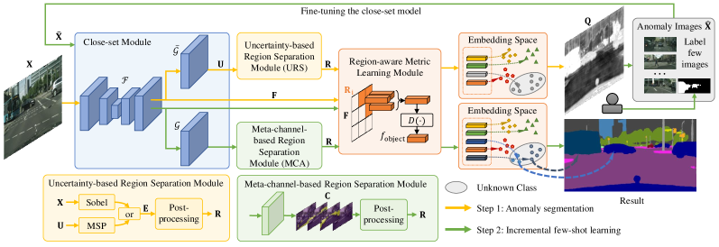
Figure 2: The pipeline of Region-aware Metric Learning for Open World Semantic Segmentation: 1) train a close-set segmentation model with known classes (bluish square); 2) Anomaly Segmentation (yellowish arrows): separate regions based on edge prediction (yellowish squares) and segment the anomaly regions using metric learning (orangish squares); 3) annotate for unknown objects ($\hat{\mathbf{X}}$) to fine-tune the close-set model; 4) Incremental few-shot learning (greenish arrows): separate regions based on MCA (greenish squares) and segment the OOD objects using metric learning (orangish squares). (Best view in color)

2.4 Metric Learning

Deep metric learning constrains the distance between feature embedding of learning samples to manipulate the feature distribution. Its applications are seen in various computer vision tasks, such as open set recognition Chen et al. (2020), few-shot learning Oreshkin et al. (2018) and open world semantic segmentation Cen et al. (2021). Classic metric learning includes two paradigms. The first is to learn with pair-wise labels, under the guidance of triplet loss  Schroff et al. (2015) and center loss Wen et al. (2016). The second consists of softmax cross-entropy and variants that train the model with class-level labels. A recently proposed method called Circle loss Sun et al. (2020) unifies the above two paradigms and forms the feature space with large inter-class distances and small intra-class distances. We thus adopt Circle loss as the key objective of our proposed RAML module.

3 Methods

As shown in Figure 2, our proposed method contains: 1) a backbone model for close-set segmentation, 2) an anomaly segmentation process to delineate the unknown regions of OOD data, and 3) an incremental few-shot learning step for splitting the unknown regions into objects with novel classes.

3.1 Close-set Segmentation Module

Suppose $\mathcal{C}_{in}=\{C_{in,1},C_{in,2},...C_{in,N}\}$ are $N$ in-distribution classes, which are all annotated in training datasets, and $\mathcal{C}_{out}=\{C_{out,1},C_{out,2},...C_{out,M}\}$ are $M$ novel classes not involved in the training datasets. Here, the semantic segmentation network $\mathcal{S}$ is divided into a feature extractor $\mathcal{F}$ and a label predictor $\mathcal{G}$, where $\mathcal{S}=\mathcal{G}\circ\mathcal{F}$.

For the close-set segmentation, we minimize the following loss $\mathcal{L}_{seg}(\mathcal{F},\mathcal{G})$ which guides $\mathcal{S}$ to produce a pixel-level segmentation for in-distribution classes.

$$\mathcal{L}_{seg}(\mathcal{F},\mathcal{G})=\mathbb{E}_{\mathbf{X},\mathbf{Y}}(\ell_{ce}(\mathcal{G}\circ\mathcal{F}(\mathbf{X}),\mathbf{Y}))$$ (1)

where $\ell_{ce}(\cdot,\cdot)$ indicates the multi-class cross entropy loss, $\mathbf{X}\in\mathbb{R}^{3\times H\times W}$ is an input image, $\mathbf{Y}$ is the corresponding label.

After training this module, we obtain a trained feature extractor $\mathcal{F}$ and a trained label predictor $\mathcal{G}$. The feature map $\mathbf{F}=\mathcal{F}(\mathbf{X})\in\mathbb{R}^{N_{1}\times H\times W}$ and the non-normalized logit $\mathbf{U}=\bar{\mathcal{G}}(\mathbf{F})\in\mathbb{R}^{N\times H\times W}$ can then be generated for in-distribution classes, where $\bar{\mathcal{G}}$ is obtained by removing the softmax layer of $\mathcal{G}$. The feature map $\mathbf{F}$ and the non-normalized logit $\mathbf{U}$ will be used in later modules.

3.2 Anomaly Segmentation

To identify the candidate regions of region-aware anomaly segmentation, we adopt an uncertainty-based OOD objects detection method, MSP Hendrycks and Gimpel (2017), as our region separation module, named Uncertainty-based Region Separation (URS). Its high uncertainty response around the object edges could be used as a promising initialization of the region separation, as shown in Figure 3.

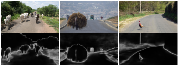
Figure 3: Visual examples of maximum softmax probability. Borders between objects have higher uncertainty because the semantics of the borders are usually ambiguous.

To further enhance the edges, we introduce Sobel filtering over the original input image. The final edge prediction map $\mathbf{E}$ can be generated as follow,

$$\mathbf{E}=\mathbb{I}\left(\operatorname{Sobel}(\mathbf{X})\geq\alpha\text{ or }\operatorname{MSP}(\mathbf{U})\geq\beta\right),$$ (2)

where $\mathbf{X}$ is the input image, $\mathbf{U}$ is the non-normalized logit, and $\mathbb{I}(\cdot)$ is an indicator function, $\alpha$ and $\beta$ are hyper-parameters to control the edge prediction. According to $\mathbf{E}$, we use a post-processing sub-module, including the hole filling and connected component algorithms, to generate the candidate regions $\mathcal{R}=\{\mathbf{R}_{1},\mathbf{R}_{2},\cdots,\mathbf{R}_{T}\}$, where $\mathbf{R}_{i}\in\{0,1\}^{H\times W}$ represents the $i$-th region.

We then propose a RAML module for anomaly segmentation to classify the candidate regions $\mathcal{R}$. For each region $\mathbf{R}_{i}\in\{0,1\}^{H\times W}$, the region-aware feature embedding is obtained as below:

$$f_{object}=\mathcal{D}(\frac{\sum_{j,k}\mathbf{F}^{j,k}\mathbf{R}_{i}^{j,k}}{\sum_{j,k}\mathbf{R}_{i}^{j,k}})\in\mathbb{R}^{N_{2}}$$ (3)

where $\mathbf{F}^{j,k}\in\mathbb{R}^{N_{1}}$ is the feature vector of pixel $(j,k)$, $\mathcal{D}(\cdot)$ consists of two fully-connected layers to control the embedding dimension. $f_{object}$ is compared to all the prototypes of the known classes by metric learning constrained by circle loss Sun et al. (2020). Specifically, the prototype of $l$-th known class $f_{l}$ can be obtained using the semantic segmentation label. Then, the region-aware anomaly probability of $\mathbf{R}_{i}$ can be expressed as below,

$$\mathcal{P}(\mathbf{R}_{i},\mathbf{F})=\max_{1\leq l\leq N}\frac{f_{object}\cdot{f_{l}}}{\|f_{object}\|\|f_{l}\|}.$$ (4)

Finally, to generate a pixel-level anomalous probability map, we combine the information from the non-normalized logit and the above region-aware anomaly probabilities. For each pixel $(j,k)$, uncertainty intensity $\mathbf{Q}^{j,k}$ is computed as,

$$\mathbf{Q}^{j,k}=-\max_{1\leq l\leq N}\ \mathbf{U}^{j,k}_{(l)}\cdot\mathcal{P}(\mathbf{R}_{i},\mathbf{F}),$$ (5)

where the pixel $(j,k)$ belongs to region $\mathbf{R}_{i}$, $\mathbf{F}$ is the feature map, $\mathcal{P}(\cdot,\cdot)$ is the region-aware anomaly probabilities. $\mathbf{U}^{j,k}_{(l)}$ is the $l$-th output of pixel $(j,k)$ in the non-normalized logit $\mathbf{U}$. We then normalize the uncertainty intensity $\mathbf{Q}^{j,k}$ for each pixel to obtain the anomalous probability map, which is used to identify the unknown regions in the image.

3.3 Incremental Few-shot Learning via MCA

After the anomaly segmentation, open world semantic segmentation requires the model to identify all objects of $M$ novel classes in the unknown regions. One way to realize the incremental few-shot learning is to use a few labeled images containing objects with novel classes to fine-tune the close-set segmentation model under the loss $\mathcal{L}_{seg}$. However, experiments show that this improvement is trivial. We thus propose an innovative MCA module for further creating sub-regions in the unknown regions from anomaly images $\hat{\mathbf{X}}$. MCA takes the prediction of the label predictor $\mathcal{G}$ in the close-set model as its input to output $(N+K)$ channels with softmax activation $\mathbf{C}\in[0,1]^{(N+K)\times H\times W}$. The first $N$ channels are the segmentation results for all in-distribution classes, while the last $K(K>M)$ channels are meta channels to overly segment the unknown regions. Several MCA-related losses are integrated into $\mathcal{L}_{seg}$ during the fine-tuning, and the overall loss function is,

$$\mathcal{L}_{overall}=\mathcal{L}_{seg}+\lambda_{inter}\mathcal{L}_{inter}+\lambda_{split}\mathcal{L}_{split}+\lambda_{rec}\mathcal{L}_{rec}.$$ (6)

The first term $\mathcal{L}_{seg}$ is the segmentation loss for all in-distribution classes from Equation 1. The second term utilizes the negative of Dices to minimize the intersection between any pairs of output channels, which is defined as:

$$\mathcal{L}_{inter}=\sum_{1\leq i<j\leq N+K}(1-\ell_{dice}(\mathbf{C}_{i},\mathbf{C}_{j}))$$ (7)

where $\ell_{dice}(\cdot,\cdot)$ indicates the dice loss and $\mathbf{C}_{i}$, $\mathbf{C}_{j}$ are the $i$-th and $j$-th channels of the segmentation output.

The third term aims to avoid the sub-regions (candidates of OOD objects) gathering in a few certain channels:

$$\mathcal{L}_{split}=\sum_{i=N+1}^{N+K}-\log(\max(\eta\sum_{j,k}\mathbf{C}^{j,k}_{i},1))$$ (8)

where $\mathbf{C}^{j,k}_{i}$ represent $(j,k)$ pixel output of $i$-th channel and $\eta$ is a hyper-parameter to control the separation. $\mathcal{L}_{split}$ reaches the minimum when the sub-regions scatter across the output channels according to Jenson’s inequality.

The last term encourages the outputs of all channels to reconstruct the entire image, further avoiding loss of information:

$$\mathcal{L}_{rec}={||\mathbf{X}\odot(\sum_{i=1}^{N+K}\mathbf{C}_{i}-\mathbbm{1}_{H\times W})||^{2}}$$ (9)

where $\odot$ is the element-wise multiplication operator and $\mathbbm{1}_{H\times W}$ is a matrix with all ones.

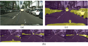
Figure 4: Visualization results of MCA. (a) Input image; (b) Meta-channel response ($K=4$); (c) Aggregated Meta-channel.

As shown in Figure 4, we observe that MCA tends to segment objects based on local semantic information. One unknown object may be segmented into more than one channel and lose completeness. (e.g., The windows and wheels of cars may be divided into different channels.) Therefore, we aggregate the sub-regions from certain meta channels according to few-shot (here $L$-shot) labeled images, which generates the candidate regions $\mathcal{R}=\{\mathbf{R}_{1},\mathbf{R}_{2},\cdots,\mathbf{R}_{T}\}$ for the final RAML module of incremental few-shot learning.

Similar to Equation 3, the region-aware feature embedding $f_{object}$ for each region $\mathbf{R}_{i}$ could be computed. The prototype of $i$-th unknown class ($1\leq i\leq M$) from $L$-shot newly labeled images is defined as:

$$c_{i}=\frac{1}{L}\sum_{j=1}^{L}f_{i}^{(j)}$$ (10)

where $f_{i}^{(j)}$ represents the feature embedding of $i$-th unknown class in $j$-th annotated image. For each region-aware feature embedding $f_{object}$, we use cosine similarity to measure the distance between this candidate region and every unknown class:

$$s_{object}^{i}=\frac{f_{object}\cdot{c_{i}}}{\|f_{object}\|\|c_{i}\|},i=1,2,...,M$$ (11)

The candidate region can be classified as the $i$-th novel class $C_{out,i}$ only if the cosine similarities satisfy the following two criteria:

$$\left\{\begin{array}[]{cc}s_{object}^{i}>\theta_{novel}\\ s_{object}^{i}>s_{object}^{i^{\prime}}&\forall i^{\prime}\neq i\end{array}\right.$$ (12)

where $\theta_{novel}$ is a hyper-parameter to control classification.

4 Experiments

Our experiments include three parts: (1) experimental results of anomaly segmentation in subsection 4.1; (2) experimental results of incremental few-shot learning results in subsection 4.2; (3) ablation studies in subsection 4.3 and Appendix.

4.1 Anomaly Segmentation

Figure 5: Visualization results of anomaly segmentation on Road Anomaly. (a) input image; (b) ground truth; (c) edge prediction; (d) results of MaxLogit Hendrycks et al. (2019). (e) results of our proposed RAML method. For (d) and (e), higher value represents greater probability of anomaly. The red bounding boxes indicate that RAML ensures the integrity of the anomaly regions.

Datasets.

7000 full-frame annotated driving scenes from BDD100k Yu et al. (2020) are used to train the close-set segmentation model, containing 19 categories of objects as in-distribution objects. For anomaly segmentation, we use another two road scene datasets, Lost and Found Pinggera et al. (2016) and Road Anomaly Lis et al. (2019), with anomalous objects other than ones in BBD100k.

Implementation details.

We follow Hendrycks et al. (2019); Cen et al. (2021) to use PSPNet as the network backbone of our close-set segmentation module and apply two fully connected layers for RAML. We follow Hendrycks and Gimpel (2017) to use three metrics to evaluate the performance of anomaly segmentation, including area under ROC curve (AUROC), area under the precision-recall curve (AUPR), and the false-positive rate at 95% recall (FPR95).

Results.

As shown in Table 1, our proposed RAML module achieves the SOTA performance on Lost and Found and Road Anomaly for anomaly segmentation. Figure 5 presents some visual examples to compare RAML and the pixel-wise method. The proposed RAML module produces higher response values and better integrity within the anomalous objects, significantly reducing the false-negative cases.

Dataset	Lost and Found			Road Anomaly
Method	AUPR$\uparrow$	AUROC$\uparrow$	FPR95$\downarrow$	AUPR$\uparrow$	AUROC$\uparrow$	FPR95$\downarrow$
Ensemble	-	57	-	-	67	-
RBM	-	86	-	-	59	-
MSP	21	83	31	19	70	61
MaxLogit	37	91	21	32	78	49
DUIR	-	93	-	-	83	-
DML	45	97	10	37	84	37
RAML(Ours)	46	97	8	42	86	32

Table 1: Results of anomaly segmentation on Lost and Found and Road Anomaly.

4.2 Incremental Few-shot Learning

Datasets.

we use Cityscapes dataset to train and evaluate our RAML module in the incremental few-shot learning step. Cityscapes consists of 2975 real-world images in the training set and 500 in the validation set with a resolution of $2048\times 1024$. The division of training set and test set in our experiments is consistent with this division.

Implementation details.

We follow Cen et al. (2021) to train a DeeplabV3+ model as the close-set model, which is followed by two fully connected layers for RAML and use mean Intersection-over-Union (mIoU) to evaluate the performance of segmentation results. Specifically, mIoUold and mIoUnovel are the mIoUs of known and unknown classes, respectively. The metric mIoUharm is a comprehensive index Xian et al. (2019) that balances mIoUold and mIoUnovel.

Figure 6: t-SNE visualization for (a) pixel-wise NPM method and (b) our proposed RAML method. All learned metrics of 19 classes of the Cityscapes dataset are included, where car, truck and bus are OOD classes.

16+1 setting	Method	road	sidewalk	building	wall	fence	pole	traffic light	traffic sign	vegetation	terrain	sky	person	rider	train	motorcycle	bicycle	car	truck	bus	mIoUall	mIoUnovel	mIoUold	mIoUharm
Baseline	All 17	97.8	82.4	91.8	52.3	57.5	59.9	64.1	74.2	91.9	61.4	94.6	79.4	58.8	75.6	61.7	74.9	94.8	-	-	74.9	-	-	-
	First 16	98.0	82.1	91.4	43.6	56.4	58.9	61.4	72.6	91.6	60.5	94.4	79.1	57.6	67.9	61.1	75.1	-	-	-	72.0	-	-	-
	FT	0.0	0.0	0.0	0.0	0.0	0.0	0.0	0.0	0.0	0.0	0.0	0.0	0.0	0.0	0.0	0.0	6.6	-	-	0.4	6.6	0.0	0.0
5 shot	PLM	97.1	79.3	89.2	41.9	55.3	57.5	60.8	71.0	91.1	59.4	93.9	73.3	49.2	34.2	14.3	51.8	75.7	-	-	64.4	75.7	63.7	69.2
	NPM	96.2	79.3	89.2	41.6	52.0	56.3	61.1	69.4	90.4	58.8	94.1	74.4	55.3	53.4	39.2	70.3	64.6	-	-	67.4	64.6	67.6	66.1
	RAML(Ours)	97.3	82.6	91.4	51.0	57.2	59.2	65.5	74.4	91.7	63.9	94.7	79.1	59.1	23.7	52.1	72.3	85.2	-	-	70.6	85.2	69.7	76.7
1 shot	PLM	96.8	77.1	89.6	41.4	48.7	53.2	60.3	64.5	90.3	55.6	94.3	59.1	43.6	39.5	12.0	35.7	64.5	-	-	60.4	64.5	60.1	62.2
	NPM	95.9	79.2	88.8	41.3	50.5	56.0	61.0	69.1	90.2	58.6	94.1	73.6	55.1	49.7	37.4	69.6	60.1	-	-	66.5	60.1	66.9	63.3
	RAML(Ours)	97.4	82.6	91.5	51.0	57.3	59.3	65.5	74.4	91.8	64.0	94.7	79.2	59.1	11.5	52.2	72.4	85.5	-	-	70.0	85.5	69.0	76.4
16+3 setting
Baseline	All 19	97.9	83.0	91.7	51.5	58.3	59.8	64.2	74.2	92.0	61.2	94.6	79.7	59.1	63.9	61.5	75.0	94.2	78.5	81.4	74.8	-	-	-
	First 16	98.0	82.1	91.4	43.6	56.4	58.9	61.4	72.6	91.6	60.5	94.4	79.1	57.6	67.9	61.1	75.1	-	-	-	72.0	-	-	-
	FT	0.0	0.0	0.0	0.0	0.0	0.0	0.0	0.0	0.0	0.0	0.0	0.0	0.0	0.0	0.0	0.0	0.0	0.0	0.4	0.0	0.1	0.0	0.0
5 shot	PLM	97.1	79.2	84.8	38.1	46.4	56.8	58.8	61.0	91.0	59.3	92.9	63.6	47.5	3.4	13.8	47.5	67.0	5.7	12.0	54.0	28.2	58.8	38.1
	NPM	96.1	79.3	58.7	41.5	51.5	56.3	60.7	69.0	90.4	58.8	94.1	74.3	55.1	32.0	39.1	70.2	55.7	1.6	21.0	58.2	26.1	64.2	37.1
	RAML(Ours)	97.3	82.6	91.1	50.6	57.2	59.1	65.5	74.1	91.7	64.0	94.7	79.0	58.9	3.7	52.2	72.3	79.3	9.7	26.0	63.6	38.4	68.4	49.1
1 shot	PLM	96.8	75.2	49.0	33.1	31.4	48.0	33.2	44.6	89.7	55.3	23.0	42.1	32.8	5.3	8.0	27.7	30.4	0.7	9.5	38.7	13.5	43.4	20.6
	NPM	95.8	79.2	44.6	41.2	50.2	56.0	60.5	67.5	90.1	58.6	94.0	73.5	54.9	24.9	37.2	69.6	54.5	1.1	22.0	56.6	25.9	62.3	36.5
	RAML(Ours)	97.4	82.6	91.3	50.3	56.0	59.2	65.5	74.1	91.7	63.9	94.7	79.1	58.9	3.9	52.2	72.4	80.9	5.5	23.0	63.2	36.5	68.3	47.5

Table 2: Incremental few-shot learning results on Cityscapes for 16+1 setting (OOD class is car) and 16+3 setting (OOD classes are car, truck, bus). The unknown classes are in blue. Finetune (FT) is the baseline with catastrophic forgetting.

Figure 7: Ablation study of the ratio of unknown classes to known classes. We compare our method to NPM and report results with mIoUnovel and mIoUharm.

Figure 8: Visual examples of RAML for open world semantic segmentation: (a) input images. (b) ground truth. (c) close-set outputs. (d) anomaly segmentation outputs. (e) MCA outputs. (f) results of pixel-wise NPM Cen et al. (2021). (g) results of our RAML module. Yellow boxes indicate that RAML method can better ensure the integrity of the OOD objects. For example, in the first row, the pixel-wise method mistakenly divides the wheels of the bus into cars, while RAML can correctly segment the entire bus. (Best view in color and zoom in.)

Results.

We test our method on CityScapes and compare our method to pixel-wise NPM and PLM proposed by Cen et al. (2021). In our experiment, car, truck, and bus are 3 OOD classes not involved in the training stage while the other 16 classes are regarded as in-distribution classes. As shown in Table 2, our proposed RAML module outperforms the previous methods with a relatively large margin. According to Figure 8, pixel-wise metric learning shows erroneous broken segmentation results on OOD objects, while the proposed RAML demonstrates a remarkable ability to maintain the integrity of these results. In addition, Figure 6 shows that the feature embeddings produced by the proposed RAML maintain a reasonable inter-class distance and their intra-class distributions are also more concentrated. Such feature distribution could foster the model to obtain a robust decision boundary.

4.3 Ablation Study

Ratio of unknown classes to known classes.

The performance of the trained segmentation model has highly correlated with the amount of training information. We compare our proposed RAML method with the current SOTA method, NPM Cen et al. (2021), under the different ratios of unknown classes to known classes. As shown in Figure 7, although our RAML method has a decline in performance as the ratio increases, it outperforms NPM in all ratio settings.

Method	mIoUall	mIoUnovel	mIoUold	mIoUharm
Baseline	49.1	1.5	58.0	2.9
$+L_{rec}$	61.8	33.6	67.1	43.2
$+L_{rec}+L_{split}$	62.6	37.6	67.3	48.3
$+L_{rec}+L_{split}+L_{inter}$	63.6	38.4	68.3	49.1

Table 3: Ablation study of losses used in MCA Module. Baseline is using Close-set Module directly.

Losses in MCA.

This section evaluates the losses of our MCA module. As shown in Table 3, the reconstruction loss ensures that our model obtains all information for the unknown classes, significantly improving the validity of MCA. The intersection loss and split loss also bring relatively smaller gains by improving the distribution of candidate regions in meta channels.

5 Conclusion

We have proposed RAML to enhance the performance of open world semantic segmentation. The main reason is that the region-aware feature outperforms the pixel-wise feature on maintaining the semantic integrity of the segmented OOD objects. Effective region separation methods are needed to realize RAML on anomaly segmentation and incremental few-shot learning. We, therefore, adopt the classic uncertainty-based methods to extract candidate regions for anomaly segmentation and propose an MCA module to further separate the anomaly regions for incremental few-shot learning. Experimental results show that our proposed method achieves the SOTA performance on the anomaly segmentation and the overall open world semantic segmentation. Our method has the potential to boost the use of open world semantic segmentation in practical applications.

6 Acknowledgments

This work is supported by the Grants under the National Natural Science Foundation of China (NSFC) under Grants 12090022, 11831002, 71704023, and Beijing Natural Science Foundation (Z180001).

Appendix

Appendix A Abbreviations

RAML: Region-Aware Metric Learning.

MCA: Meta-Channel Aggregation.

URS: Uncertainty-based Region Separation.

DMLNet: Deep Metric Learning Network.

PML: Pixel-wise Metric Learning.

NPM: Novel Prototype Method.

PLM: Pseudo Label Method.

OOD: Out-Of-Distribution.

MSP: Maximum Softmax Probability.

MaxLogit: Maximum Logit.

All 17: Using 17 classes for full-supervised learning.

All 19: Using 19 classes for full-supervised learning.

First 16: Only using 16 known classes for close-set segmentation with full-supervised learning.

FT: Using unknown novel images for fine-tuning close-set segmentation model.

Appendix B Anomaly Segmentation

B.1 Details for expression 5

For a new image $\mathbf{X}$ containing OOD objects, the uncertainty intensity Q is calculated as follows: 1) The close-set segmentation model infers the image $\mathbf{X}$ and produces the non-normalized logit $\mathbf{U}=\bar{\mathcal{G}}\circ\mathcal{F}(\mathbf{X})$ (Section 3.1). The small $\mathbf{U}$ value of a pixel means that it is more likely to belong to an unknown region. 2) We use a URS module to divide $\mathbf{X}$ into multiple regions, and the region-aware embeddings are calculated for each of them (expression (3)). 3) RAML computes the similarity between these region-aware embeddings and those of the known classes from the training set to obtain the maximum similarity $\mathcal{P}$ (expression (4)). If the maximum similarity is small, the region does not belong to any known classes. 4) Combining the results of 1) and 3), we take the product of $\mathbf{U}$ and $\mathcal{P}$. The negative of this product, named uncertainty intensity $\mathbf{Q}$, is thus positively related to the probability that a certain region is unknown.

B.2 Implementation Details

We use PyTorch (version 1.8.2) to implement our model and run it in the environment of CUDA 11.0. For anomaly segmentation, we follow Hendrycks et al. [2019]; Cen et al. [2021] to use PSPNet Zhao et al. [2017] with ResNet101 He et al. [2016] as the close-set segmentation module. We set the batch size to 6 and train the model on two RTX-3090s in parallel. Moreover, we follow Cen et al. [2021] to train the module using SGD as the optimizer with a momentum of 0.9, a learning rate of $2\times 10^{-2}$, and a learning rate decay of $10^{-4}$.

We build the RAML module by applying two fully connected layers (4846 units and 128 units, respectively) after the close-set segmentation module, as shown in Figure 2. We train the module for 1500 iterations with a batch size of 6. Other training parameters are the same as the close-set segmentation module mentioned above.

In addition, Sobel filtering Sobel and Feldman [1968] compensates the low sensitivity of MSP Hendrycks and Gimpel [2017] on the edges of small objects. In the experiments, we set the hyper-parameters $\alpha$ and $\beta$ in Equation 2 as 50 and 0.7 for Lost and Found, and 150 and 0.4 for Road Anomaly.

Appendix C Incremental Few-shot Learning

This section introduces implementation details and more ablation studies of the incremental few-shot learning of our proposed RAML method.

C.1 Implementation Details

We follow Cen et al. [2021] to use a DeeplabV3+ model as the backbone of our close-set model. In the MCA module, We set $K=4$, $\eta=0.02$, $\lambda_{inter}=0.1$, $\lambda_{split}=0.1$ and $\lambda_{rec}=0.01$. In our metric leanring, we set $\theta_{novel}=0.8$ as the cosine threshold for the unknown objects, $N_{1}=256,N_{2}=128$ in embedding space, $m=0.25$ and $\gamma=8$ in circle loss Sun et al. [2020].

We train the close-set segmentation model for $3\times{10}^{4}$ iterations. After the anomaly segmentation, we finetune the close-set segmentation model for another ${10}^{4}$ iterations with all training samples plus the few-shot novels. We then build the RAML module by applying two fully connected layers (256 units and 128 units, respectively) after the MCA module, as shown in Figure 2. The RAML module is trained for $10^{4}$ iterations.

In all training stages, we use an SGD optimizer with a momentum of 0.9, a learning rate decay of $10^{-4}$, and an initial learning rate of 0.01 for the feature extractor and 0.1 for the label predictor, respectively. Poly learning rate scheduler is used with the power of 0.9 for one epoch. Due to the GPU memory limitation, we set crop size to 762 in the close-set segmentation model and MCA module, and we further resize the feature maps to 512 in the RAML module. The batch size is set to 6.

C.2 Implementation Details for MCA

In this section, we introduce how MCA module works in the inference stage. First, we select candiate meta channel set $\mathbf{C}_{cand}$ from annotated set $(\mathbf{X},\mathbf{Y})$. $\mathbf{C}_{meta}^{i}\in\{0,1\}^{K\times H\times W}$ is the output mask for an annotated image $(\mathbf{x}_{i},\mathbf{y}_{i})$, where $\mathbf{x}_{i}$ is the input image and $\mathbf{y}_{i}\in\{0,1\}^{H\times W}$ is the output mask for the novel class. A meta channel $\mathbf{c}^{i}_{j}$ is a candiate meta channel of meta channel output $\mathbf{C}_{meta}^{i}$ when it satify:

$$\frac{\sum_{h,w}\mathbf{c}^{i}_{j,hw}}{\sum_{h,w}\mathbf{y}_{hw}}>\kappa.$$ (13)

Here, we set $\kappa=0.1$. The candiate meta channels set $\mathbf{C}_{cand}$ for all $L$ annotated images is defined as:

$$\mathbf{C}_{cand}=\cup_{i=1}^{L}\mathbf{C}_{cand}^{i}.$$ (14)

As discussed in Section3.3. MCA module tends to segment objects based on local semantic information. Therefore, the information for novel classes is contained in the the candiate meta channel set $\mathbf{C}_{cand}$. In the inference stage, we aggregate the sub-regions from $\mathbf{C}_{cand}$ and get the output mask $\mathbf{C_{out}}$ via the exclusive disjunction of all $n$ channels in $\mathbf{C}_{cand}$, which can be expressed as:

$$\mathbf{C_{out}}=\mathbf{1}-(\mathbf{1}-\mathbf{c}_{1})\odot(\mathbf{1}-\mathbf{c}_{2})\odot\cdots\odot(\mathbf{1}-\mathbf{c}_{n}).$$ (15)

Then we use a post-processing algorithms on $\mathbf{C}_{out}$, including the hole filling and connected component algorithms, to generate the candidate regions $\mathcal{R}$ described in Section3.3.

C.3 An example for RAML module

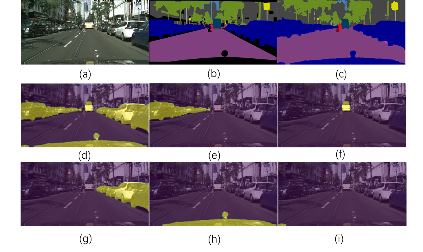
Figure I: A Visual example of RAML Module in 16+3 setting. (a) Input image. (b) Ground truth. (c) Open World Semantic Segmentation output. (d) Aggregated Meta-channel. (e)-(i) Candidate regions.

Figure I shows an example for our proposed RAML method. In this case, MCA separates the anomaly regions into 5 candidate regions for the final stage of incremental few-shot learning. After that, the RAML module computes the region-aware feature embedding $f_{object}$ for each region according to Equation 3 and classifies it as a certain novel class according to Equation 12. As shown in Table D, the RAML module correctly classifies the unknown classes even there’s more than one cosine similarity above the threshold $\theta_{novel}$. Besides, we notice that RAML can classify Regions (h) and (i) in Figure I correctly which are ignored in the labels of CityScapes dataset.

Candidate Region	Output	Car	Truck	Bus
(e)	Car	0.97	0.82	0.92
(f)	Bus	0.87	0.75	0.93
(g)	Car	0.97	0.77	0.92
(h)	Car	0.91	0.65	0.69
(i)	Car	0.80	0.48	0.57

Table D: Classification output for RAML module on the example in Figure I. Cosine similarity is reported between each pair of candidate regions of the unknown classes in 16+3(car,truck,bus) settings where $\theta_{novel}=0.8$.

C.4 Details for Circle Loss

Circle loss was proposed by Sun et al. [2020], which offers a unified formula for both two deep metric learning paradigms, i.e., learning with class-level labels and pair-wise labels. Meanwhile, it provides a a more flexible optimization way towards a more definite convergence aim. Because of its superiority in metric learning, we adopt it in our RAML module.

Formally, given a region-aware feature embedding $f_{object}$, suppose that there are $K$ intra-class similarity scores, and $L$ inter-class similarity scores corresponding to $f_{object}$. We denote them as $\{s_{p}^{i}\}(i=1,2,\cdots,K)$ and $\{s_{n}^{i}\}(i=1,2,\cdots,L)$. The circle loss can be expressed as:

$$\mathcal{L}_{circle} =\log\left[1+\sum_{i=1}^{K}\sum_{j=1}^{L}\exp\left(\gamma\left(s_{n}^{j}-s_{p}^{i}+m\right)\right)\right]$$ (16)

$$=\log\left[1+\sum_{j=1}^{L}\exp\left(\gamma\left(s_{n}^{j}+m\right)\right)\sum_{i=1}^{K}\exp\left(\gamma\left(-s_{p}^{i}\right)\right)\right],$$

where $\gamma$ is scale factor and $m$ is a margin for better similarity separation. We set $\gamma=8.0$ and $m=0.25$ in this work.

C.5 Ablation study of region separation methods

$K$ is the number of meta channels as discussed in Section 3.3. We compare our method with different $K$s to the pixel-wise methods and our proposed Uncertainty-based method (URS). As shown in Table E, region-aware methods perform consistently better than pixel-wise methods. The model performs best when $K=4$ and a reasonable explanation is that an overly small $K$ shrinks the benefit from the multiple meta channels over-segmenting the anomaly regions, but an overly large $K$ may cause excessive candidates for region separation, which are more challenging to be aggregated correctly.

16+3 settings	mIoUall	mIoUnovel	mIoUold	mIoUharm
PLMlatest	19.3	17.1	19.7	18.3
PLMall	38.7	13.5	43.4	20.6
NPM	56.6	25.9	62.3	36.5
URS	60.4	26.7	66.7	38.1
MCA ($K=2$)	61.0	34.7	65.9	45.5
MCA ($K=4$)	63.2	36.5	68.3	47.5
MCA ($K=6$)	59.7	33.1	64.7	43.8

Table E: Ablation study of region separation methods, including pixel-wise method, RAML with our proposed URS module, and RAML with our proposed MCA module with different numbers of meta channels.

16+3 settings	${\theta}_{novel}$	mIoUall	mIoUnovel	mIoUold	mIoUharm
5 shot	0.7	63.3	37.6	68.2	48.4
	0.75	63.5	38.1	68.3	48.9
	0.8	63.6	38.4	68.4	49.1
	0.85	63.9	38.1	68.7	49.0
	0.9	64.1	37.2	69.2	48.4
1 shot	0.7	63.2	36.1	68.3	47.2
	0.75	63.3	36.4	68.3	47.5
	0.8	63.3	36.5	68.3	47.5
	0.85	64.1	36.4	69.4	47.7
	0.9	63.3	32.5	69.1	44.2

Table F: Ablation study of cosine similarity threshold $\theta_{novel}$

C.6 Ablation study of cosine similarity threshold

$\theta_{novel}$ controls the cosine similarity threshold for unknown classes as discussed in Section 3.3. As shown in Table F, large $\theta_{novel}$ will improve the precision rate for unknown classes while reducing the recall rate on them (shown as the performance drop on known classes). To balance the performance on known classes and unknown classes, we select $\theta_{novel}=0.8$.

C.7 Ablation study of Novel selection

As shown in Table G, the selection of novels affects the segmentation performance, which is more obvious in 1-shot settings. As only a few data are labeled as novels, their center embedding may drift heavily from the overall data distribution. It is worth noting that for a fair comparison, our results reported in Table 2 adopt a fixed way of selecting novels, which follows Cen et al. [2021] to choose the images with the largest area of the unknown classes as novels.

16+1 settings	mIoUall	mIoUnovel	mIoUold	mIoUharm
5 shot	70.53 $\pm$ 0.32	85.51 $\pm$ 0.32	69.59 $\pm$ 0.30	76.75 $\pm$ 0.30
1 shot	70.28 $\pm$ 0.51	84.43 $\pm$ 1.58	69.52 $\pm$ 0.49	76.32 $\pm$ 0.38
16+3 settings
5 shot	63.67 $\pm$ 0.17	38.4 $\pm$ 0.68	68.42 $\pm$ 0.10	49.19 $\pm$ 0.58
1 shot	63.13 $\pm$ 0.39	35.81 $\pm$ 2.23	68.28 $\pm$ 0.07	46.93 $\pm$ 1.92

Table G: Ablation study of novel selection. We randomly select 1 or 5 novels for 5 times and report mean and std of the mIoUs.

References

- Baur et al. [2018] Christoph Baur, Benedikt Wiestler, Shadi Albarqouni, and Nassir Navab. Deep autoencoding models for unsupervised anomaly segmentation in brain mr images. In MICCAI Brainlesion Workshop, pages 161–169, 2018.
- Bendale and Boult [2015] Abhijit Bendale and Terrance Boult. Towards open world recognition. In CVPR, pages 1893–1902, 2015.
- Cen et al. [2021] Jun Cen, Peng Yun, Junhao Cai, Michael Yu Wang, and Ming Liu. Deep metric learning for open world semantic segmentation. In ICCV, pages 15333–15342, 2021.
- Chan et al. [2021] Robin Chan, Matthias Rottmann, and Hanno Gottschalk. Entropy maximization and meta classification for out-of-distribution detection in semantic segmentation. In ICCV, pages 5128–5137, 2021.
- Chen et al. [2020] Guangyao Chen, Limeng Qiao, Yemin Shi, Peixi Peng, Jia Li, Tiejun Huang, Shiliang Pu, and Yonghong Tian. Learning open set network with discriminative reciprocal points. In ECCV, pages 507–522, 2020.
- Gal and Ghahramani [2016] Yarin Gal and Zoubin Ghahramani. Dropout as a bayesian approximation: Representing model uncertainty in deep learning. In ICML, pages 1050–1059, 2016.
- He et al. [2016] Kaiming He, Xiangyu Zhang, Shaoqing Ren, and Jian Sun. Deep residual learning for image recognition. In CVPR, pages 770–778, 2016.
- Hendrycks and Gimpel [2017] Dan Hendrycks and Kevin Gimpel. A baseline for detecting misclassified and out-of-distribution examples in neural networks. In ICLR, 2017.
- Hendrycks et al. [2019] Dan Hendrycks, Steven Basart, Mantas Mazeika, Mohammadreza Mostajabi, Jacob Steinhardt, and Dawn Song. Scaling out-of-distribution detection for real-world settings. arXiv preprint arXiv:1911.11132, 2019.
- Hu et al. [2021] Hanzhe Hu, Jinshi Cui, and Liwei Wang. Region-aware contrastive learning for semantic segmentation. In ICCV, pages 16291–16301, 2021.
- Joseph et al. [2021] K J Joseph, Salman Khan, Fahad Shahbaz Khan, and Vineeth N Balasubramanian. Towards open world object detection. In CVPR, 2021.
- Lis et al. [2019] Krzysztof Lis, Krishna Nakka, Pascal Fua, and Mathieu Salzmann. Detecting the unexpected via image resynthesis. In ICCV, pages 2152–2161, 2019.
- Oreshkin et al. [2018] Boris N Oreshkin, Pau Rodriguez, and Alexandre Lacoste. Tadam: Task dependent adaptive metric for improved few-shot learning. In NeurIPS, 2018.
- Pinggera et al. [2016] Peter Pinggera, Sebastian Ramos, Stefan Gehrig, Uwe Franke, Carsten Rother, and Rudolf Mester. Lost and found: detecting small road hazards for self-driving vehicles. In IROS, pages 1099–1106, 2016.
- Saito et al. [2021] Kuniaki Saito, Ping Hu, Trevor Darrell, and Kate Saenko. Learning to detect every thing in an open world. arXiv preprint arXiv:2112.01698, 2021.
- Schroff et al. [2015] Florian Schroff, Dmitry Kalenichenko, and James Philbin. Facenet: A unified embedding for face recognition and clustering. In CVPR, 2015.
- Sobel and Feldman [1968] Irwin Sobel and Gary Feldman. A 3x3 isotropic gradient operator for image processing. a talk at the Stanford Artificial Project in, pages 271–272, 1968.
- Sun et al. [2020] Y. Sun, C. Cheng, Y. Zhang, C. Zhang, L. Zheng, Z. Wang, and Y. Wei. Circle loss: A unified perspective of pair similarity optimization. In CVPR, 2020.
- Wang et al. [2021] Wenguan Wang, Tianfei Zhou, Fisher Yu, Jifeng Dai, Ender Konukoglu, and Luc Van Gool. Exploring cross-image pixel contrast for semantic segmentation. In ICCV, 2021.
- Wen et al. [2016] Yandong Wen, Kaipeng Zhang, Zhifeng Li, and Yu Qiao. A discriminative feature learning approach for deep face recognition. In ECCV, pages 499–515, 2016.
- Xia et al. [2020] Yingda Xia, Yi Zhang, Fengze Liu, Wei Shen, and Alan L Yuille. Synthesize then compare: Detecting failures and anomalies for semantic segmentation. In ECCV, pages 145–161, 2020.
- Xian et al. [2019] Y. Xian, S. Choudhury, Y. He, B. Schiele, and Z. Akata. Semantic projection network for zero- and few-label semantic segmentation. In CVPR, 2019.
- Yu et al. [2020] Fisher Yu, Haofeng Chen, Xin Wang, Wenqi Xian, Yingying Chen, Fangchen Liu, Vashisht Madhavan, and Trevor Darrell. Bdd100k: A diverse driving dataset for heterogeneous multitask learning. In CVPR, pages 2636–2645, 2020.
- Yuan et al. [2020] Yuhui Yuan, Xiaokang Chen, Xilin Chen, and Jingdong Wang. Segmentation transformer: Object-contextual representations for semantic segmentation. In ECCV, 2020.
- Zhao et al. [2017] Hengshuang Zhao, Jianping Shi, Xiaojuan Qi, Xiaogang Wang, and Jiaya Jia. Pyramid scene parsing network. In CVPR, pages 2881–2890, 2017.
- Zhong et al. [2021] Zhun Zhong, Linchao Zhu, Zhiming Luo, Shaozi Li, Yi Yang, and Nicu Sebe. Openmix: Reviving known knowledge for discovering novel visual categories in an open world. In CVPR, pages 9462–9470, 2021.