The Impact of the Social Security Reforms on Welfare:
Who Benefits and Who Loses Across Generations, Gender, and Employment Type?

Abstract

Japan is facing rapid aging and the highest government debt among developed countries. We quantitatively explore the impact of social security reforms in Japan using an overlapping generations model with four types of households distinguished by gender and employment type. The results of our paper suggest that reducing social security benefits without extending the retirement age raises future generations’ welfare while lowering the current generation’s welfare. In particular, a medical and Long-term care insurance reform significantly lowers the welfare of current low-income groups: females and contingent workers. In contrast, a reform reducing the pension replacement rate leads to a more significant decline in the welfare of regular workers than contingent workers. Combining social security reforms with an extension of the retirement age would mitigate the declining welfare of the current generation by about 3 to 4%.

Keywords: social security reform, medical and long-term care, life cycle, demographic transition

JEL Classification: E21, H55, I13, J11

1 Introduction

Many developed countries are facing population aging. In particular, Japan is aging significantly faster than the rest of the world. In 2018, Japan’s elderly population ratio (the ratio of the population aged 65 and over to the population aged 15–64) was 47.2%. In addition, the United Nations’ projection of the ratio in 2065 shows that it is expected to be the highest among developed countries (medium projection), at around 75% in Japan and more than 80% in South Korea, where the population has been aging rapidly in recent years.

Population aging significantly changes the future distribution of the population. Figure 1 shows the population distribution in Japan in 2015 and in 2065 based on the projections from the National Institute of Population and Social Security Research (IPSS). The population distribution in 2015 has two peaks (blue line). These are the baby boomer generation and the children of the baby boomer generation. As of 2020, many of the baby boomers who began reaching the age of 65 in 2015 will already be public pensioners. Meanwhile, the junior baby boomers are the labor force. However, around 2040, the latter will also reach the retirement age of 65 and begin receiving public pensions. As a result, the total amount of pension payments could rise significantly from the late 2030s to the 2070s, according to government projections.

In addition, the population decline associated with graying leads to a decrease in the labor force. According to the projection by the IPSS, the population aged 20–64, consisting mainly of workers, will decrease monotonically in the future, while the population aged 65 and over, consisting mainly of retirees, will increase, as shown in Figure 2 Panel (a). This trend is reflected clearly in the transition of the old-age dependency ratio. While this ratio was about 50% in 2015, it is projected to exceed 80% by around 2050, shown in Figure 2 Panel (b). Because these demographic changes will exert significant impacts on the public pension and the medical and LTC insurance systems, this topic must be considered as one of the most urgent challenges on the policy agenda in terms of fiscal sustainability.

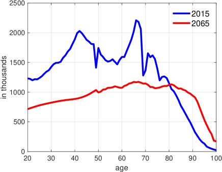
Figure 1: Change in the population distribution in Japan: from 2015 to 2065

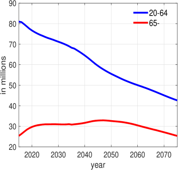
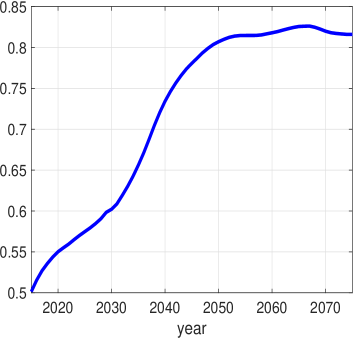
(a) Demographic change                       (b) Dependent rate

Figure 2: Demographic transition in Japan: 2015–2075

In response to the IPSS projection, the Japanese government has been reforming various social security systems, especially the public pension, medical insurance, and long-term care (LTC) insurance which run on a pay-as-you-go (PAYG). For example, the government has raised the retirement age for public pension benefits, introduced the "macroeconomic slide" to adjust the benefit levels gradually, and promoted measures to control medical costs by consolidating hospital beds based on the plan for appropriate medical care expenditures. Because the government debt resulting from these costs of social security expenditures has accumulated enormously over the years, casting a dark shadow on fiscal sustainability, reconciling them is a challenge for fiscal policy.

Since the 2000s, the government debt to GDP ratio has been the highest among developed countries, standing at 237.16% as of 2018.

Purpose and contribution of our paper

To tackle these challenges, we compare and evaluate changes in social welfare by selecting one of several options for social security reforms subject to the fiscal sustainability constraint, following McGrattan and Prescott (2017). To measure the effects of aging and public pension reform in the U.S., they use a general equilibrium overlapping generations (OLG) model with four types of households distinguished by wealth class. The feature of their model is rich parameterization, which enables calibration corresponding to both macro-level data and micro-level income data, for example the application of the progressive tax bracket to the labor income tax rate. By applying their model to Japanese policy reforms, our study provides an empirical outcome in more practical situations than previous Japanese studies.

We also extend the model of McGrattan and Prescott (2017) to four types of households distinguished by gender (male and female) and employment types (regular and contingent worker), as well as including medical and LTC insurance besides public pensions. We then quantitatively analyze the impact of social security reforms associated with a decreasing population on the welfare of different generations: the current working, retired, and future generations.

In our paper, reforms of the pension, medical insurance, and LTC insurance are considered according to two scenarios: (1) a baseline scenario based on the current system, (2) a scenario with the extension of the retirement age from 65 to 70. Within these two scenarios, we simulate three options for the reform: (1) a reform to lower the pension income replacement rate gradually from the current 62% to 50.8% by 2047; (2) a reform to raise the copayment rate for medical expenses for the elderly uniformly to 30% for all ages; and (3) a reform to increase the copayment rate for LTC expenses uniformly to 30%.

According to our simulation, by the mid-2040s, when the population and output levels are at their lowest, the output will be about 75% of its 2020 level, and extending the retirement age and reforming social security systems will have little effect on increasing the GDP. However, extending the retirement age will improve the welfare of the current generations in particular. Focusing on social security reforms, the reduction in the pension income replacement rate will reduce the welfare of regular workers by a relatively large amount, and the increase in the copayment rate for medical and LTC expenditures will lower the welfare of the current retired generation. We also find that medical and LTC insurance reform will significantly lower the welfare of females and contingent workers with relatively low incomes and assets.

The contributions of our study are as follows. The first is to quantify which characteristics of households are more significantly negatively affected in reforming the social security system needed for fiscal sustainability. The second is to simulate the impact of the two scenarios and the three social security reforms on household welfare, distinguishing between generations and types of households. Our simulations allow us to provide more practical policy implications.

The rest of this paper is organized as follows. Section 2 summarizes the institutional background of Japanese social security system and shows the contribution of this study to the previous research. Section 3 describes our model. Section 4 explains the calibration and parameterization based on the data and institutional background for the analysis, and calculates the steady state. Section 5 computes the transition path based on the steady state. Then, we conduct simulations setting the various scenarios and social security reforms described above. Section 6 discusses the conclusions of our paper and suggests future research.

2 Background and related literature

In this section, we describe two factors that provide the motivation and background for our study. First, we present the demographic data and medical and LTC expenditures per capita to clarify the arguments on which our paper focuses. Second, we summarize the literature review for the relevant field, in particular for Japan.

2.1 Institutional Background

In Japan, citizens are required to be covered by some form of public medical insurance. As of 2021, the copayment rate for medical expenses is set at 30% for those under 70 years old, 20% for those between 70 and 75 years old, and 10% for those over 75 years old (preschool children under 6 years old are required to pay 20%). However, due to the passing of a revised law on June 4, 2021, it was agreed that the copayment for those aged 75 and over will be rised to 20% in the latter half of 2022, to reduce the burden on the covered persons in the medical insurance system. In addition, LTC insurance is mandatory from the age of 40. The copayment rate for LTC expenditures is set at 10% for everyone aged 40 and over (Figure 3).

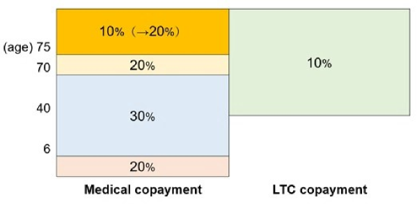
Figure 3: Medical and LTC copayment rate

Public LTC insurance was introduced in Japan in 2000. Afterward, there were increasing concerns about the financial sustainability of LTC insurance with the aging of the population, and the program has been reformed frequently since then. After introducing public LTC insurance, the number of users of LTC services, certified by the level of care required, more than tripled from 2.18 million in 2000 to 6.58 million in 2018. Correspondingly, the cost of LTC is on the rise, so the government is trying to implement reforms reducing the LTC insurance benefits, for example limiting the utilization of services according to the level of LTC required, increasing in the copayment rate for the elderly people earning the equivalent level of income as the working-age generations, and so on.

The social security reforms to maintain fiscal sustainability could have a significant impact on aggregate flows such as consumption and savings over the household life cycle. The reforms would also affect aggregate stock variables such as capital accumulation, which form future output. Since a decreasing population and labor force could also hurt economic growth, it is necessary to examine the effect of reforms comprehensively. In fact, the outlooks isssued by the government, such as the Cabinet Office’s "Medium- and Long-Term Economic and Fiscal Outlook" and the Bank of Japan’s "Outlook for Economic and Price Conditions," indicate a slowdown in the GDP growth in recent years and a decline in the total factor productivity (TFP) growth rate. For example, the Bank of Japan’s outlook shows particularly low values ranging from 0.01–0.43% from 2015 onward. Therefore, additional social security reforms are likely to be implemented simultaneously with a decreasing population and a further slowing of economic growth. It is evident that measuring the effects of such reforms on people’s welfare, evaluated from the amount of consumption and saving behavior, could have important implications for future policy discussions. On the other hand, although the growth rates of TFP and GDP are forecasted to be lower, there is a perception that this is due to the underestimation of the magnitude of GDP. According to McGrattan (2020), intangible assets, not included in GDP, and multi-sector production significantly contribute to economic fluctuations. As we will see in more detail later, McGrattan and Prescott (2017) analyzed social security reform in an aging economy by incorporating intangibles and multiple sectors into a general equilibrium OLG model. And we follow their model and approach.

2.2 Fiscal sustainability and the declining labor force

There is a large amount of literature analyzing the impact of population aging on fiscal administration in Japan. Hansen and Imrohoroğlu (2016) analyze aging and fiscal sustainability using a neoclassical growth model. They find that a consumption tax rate of about 40% is needed to sustain the fiscal balance when reforms such as the expansion of the tax base and the reduction of social security benefits are implemented. They also show that a consumption tax rate of about 60% would be needed if those reforms are not introduced.

Braun and Joines (2015) investigate the fiscal impact of an aging population on Japan’s social security system, including public pensions, medical insurance, and LTC insurance using a general equilibrium OLG model. They also analyze the impact on fiscal sustainability of reforms such as raising the consumption tax and increasing the copayment rate for medical expenditures. They conduct policy simulations under the assumption that public finances are balanced by the consumption tax rate, and they show that consumption tax rates of 30–45% would be necessary to sustain the fiscal balance. Furthermore, they find that, if reforms to raise the copayment rate for medical expenditures for the elderly to 30% are to be implemented simultaneously, the consumption tax rate needed to sustain the fiscal balance would be around 20%.

Kitao (2015) quantitatively explores the fiscal impacts of demographic change in Japan, focusing on the pension reform. She shows that the consumption tax rate needed to maintain the public finances would rise to a maximum of nearly 50% without pension reforms, and that raising the pension starting age together with a 20% benefit reduction would result in a consumption tax rate raise of less than 30%. Furthermore, Kitao (2018) focuses on the pension reform and incorporated uncertainty about the timing of beginning reforms to reduce pension benefits into the analysis to illustrate quantitatively the welfare losses that would result from a delay in reforms.

Some studies find implications that focus on the relationship between labor market policies and fiscal sustainability. Imrohoroğlu et al. (2017) measure the effects of labor force growth due to the immigration of guest workers on fiscal sustainability and welfare changes among native Japanese people in a shrinking population. They suppose that guest workers work in Japan for a decade and return to their own country without receiving social security benefits. They conduct a scenario analysis distinguishing between high and low skill levels of guest workers, and show that an influx of high-skilled guest workers lowers the consumption tax rate in particular and improves the welfare of native Japanese people in the future. Moreover, Imrohoroğlu et al. (2019) find that not only encouraging women’s labor force participation, but also increasing women’s labor productivity, combined with social security reforms, including pensions and health and long-term care insurance, are effective for improving fiscal sustainability. In their research, they develop a detailed overlapping generations model based on Japanese micro data, which incorporates heterogeneity in household income and labor supply.

2.3 Inequality, gender, and employment type

Recent research suggests that the impact of social security reform varies by household income and wealth levels, gender, and other characteristics. McGrattan and Prescott (2017, 2018) analyze the impact of a public pension system reform from a PAYG system to a privately funded system using an OLG model with household heterogeneity characterized by four types in terms of their wealth class. They quantified the degrees to which a change to a privately funded system has improved social welfare for heterogeneous households with income and wealth inequality. To capture the gains and losses between public pension contributions and benefits over the life cycle with higher accuracy, they incorporated a progressive labor income tax rate into their model. They also incorporate into their model two firm sectors: the corporate sector and a household business (self-employment) sector, and two assets: tangible and intangible assets. These detailed settings using macro and micro data allow the model to examine various practical policy simulations focused on the inequality between heterogeneous households. Furthermore, following McGrattan and Prescott (2017), McGrattan et al. (2018) apply the model to the Japanese case and quantified studied social security reforms including those of pensions and medical and LTC insurance, by classifying types of agents into four wealth classes.

However, several studies point out that gender and employment types are essential determinants of income and wealth inequality in Japan’s labor market (e.g., Moriguchi, 2017). Moriguchi (2017) argues that the gaps in income and wealth between regular workers, who are employed long-term (or until their retirement age in most cases) and receive generous social security benefits, and contingent workers, who are not taken those benefits, is significant in Japan. Moreover, she shows the increasing share of contingent workers has contributed to the expansion of this inequality in recent years. The share of contingent workers has risen from about 10% for males and 45% for females in 2000 to about 20% for males and 52% for females in 2019. Furthermore, the wage gaps between gender and employment types have remained for several decades. Figure 4 depicts the time series in nominal hourly wages by gender and employment types from 2000 to 2019, which is based on the Basic Wage Structure Survey by the Ministry of Health, Labour and Welfare. As this figure shows, there has been little change in relationship of the wage gaps between these four types of workers for long period. Accordingly, we classify agents in terms of gender and employment types in order to conduct an analysis focusing on household heterogeneity in Japan.

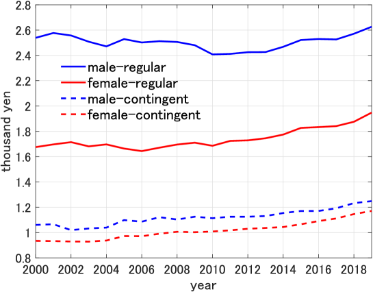
Figure 4: Time series in nominal hourly wages by type

Actually, studies regarding Japan’s social security, fiscal and taxation systems have focused their analysis on heterogeneity based on gender and employment type. For example, Kitao and Mikoshiba (2020) developed an OLG model that incorporates males and females with different employment type, labor participation rates, labor productivity, and life expectancy to examine the impact of labor market changes on fiscal sustainability. They showed that an increase in labor participation rates and labor productivity, especially of females and the elderly, could be effective for contributing to the transition away from budget deficits. Kitao and Mikoshiba (2022) quantified the effects of tax incentive policies mainly applied to married women (i.e., tax credits for their spouse’s income). They examined the extent to which the tax incentive treatment reduces women’s labor force participation and compromises them to work as low-income contingent workers. Their counterfactual simulations show that females’ labor force participation and income could increase by 12.5 and 22.7%, respectively, without these tax incentives. They suggest that removing taxation distortions to their labor force participation and choice of employment types would increase the number of females working as regular workers, which is expected to bring a marked rise in income for their households. They also discussed that the government might increase tax revenues through this tax reform without reducing the welfare of the current generations.

Of course, many researchers have also focused on gender and employment type differences in various countries outside Japan. For example, Braun et al. (2017) discuss the effective of old-age public income compensation programs by analyzing the risks of medical and LTC expenditures, spousal bereavement, and other risks faced in old age in the US that differ for males and females. Furthermore, Mukoyama et al. (2021) highlight the importance of distinguishing between full-time workers and part-timers in the labor market. They argue that the share of part-timers increased after the Great Recession in the U.S. and that the most important contributor was the transition from full-timers to part-timers. They also suggest segmenting the labor market for full-timers and part-timers is essential to reproduce the labor market dynamics during the Great Recession.

Accordingly, we classify households from gender and employment types, which might be essential determinants of Japan’s household income and wealth inequality, as well as from generations. We quantitatively analyze the heterogeneity of the impact of social security reforms between current and future generations, as well as the heterogeneity of the effects by household type distinguished by gender and employment types within a generation. In addition, the paper discusses the costs and benefits of social security reform based on the results of the quantitative analysis and derives policy implications.

2.4 Savings and medical and LTC expenditures in retirement

Turning to medical and LTC costs from different perspectives, studies have been conducted on the retirement savings puzzle, which indicates that the actual medical and LTC expenditures are higher than those derived using the standard life cycle model. For example, De Nardi et al. (2010) explain the saving behavior of elderly households in the context of precautionary savings to finance the medical expenditures that may arise during old age. In addition, Kopecky and Koreshkova (2014) find that the LTC expenditures account for a large portion of precautionary savings among the elderly. They also show that expanding Medicaid, which is the U.S. health insurance program for low-income households, could improve the welfare of future generations. Moreover, Braun et al. (2017) show that expanding social security with a means test could improve welfare by taking into account aging risks, such as death or the longevity of a spouse.

For Japan, Iwamoto and Fukui (2018) show average medical and LTC expenditures. Figure 5 depicts the per capita medical and LTC expenditures by age group. As the figure shows, medical and LTC costs are higher for the elderly. In particular, LTC costs raise rapidly after the age of 80. Increasing the expected spending in old age must influence the amount of savings and consumption at a young age. Similar to this, increases in the copayment rates for medical and LTC expenditures could have a much greater impact on them at a young age. We take the impact of such cost-up into account in our study, by incorporating both the medical and LTC costs into our model.

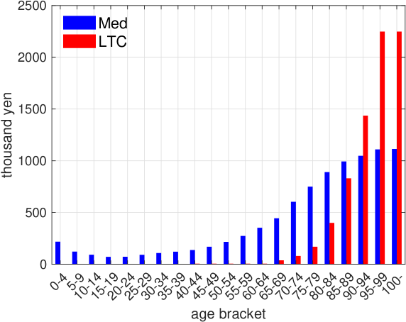
Figure 5: Per capita medical and LTC expenditure

3 Model

In this section, we describe the model used in our quantitative analysis. First, we present the settings that describe the social security system. Next, we set up households and firms, and describe the budget constraints of the government managing the social security system. Finally, we define the equilibrium conditions.

As mentioned in the previous section, our model is a deterministic OLG model following McGrattan and Prescott (2017) modified to fit Japan’s original system. The households consist of four types of agents distinguished by gender and employment type. The firms are divided into two sectors, specifically the corporate sector, and the household business (self-employment) sector, the capital of which is formed from tangible and intangible assets. The government runs the social security systems (pensions, medical insurance, and LTC insurance) as well as conducting finance by issuing government bonds and provides benefits for households.

We suppose that households make decisions with perfect foresight and that representative firms in both sectors produce with a constant return to scale technology under perfect competition. The government implements a credible fiscal policy. Time is discrete, and one period in the model is one year. We also suppose that the economy is on a balanced growth path with a constant labor-augmented productivity growth rate $\gamma$ and a constant population growth rate $n$ in the long-run.

3.1 Social security system

3.1.1 Demography

First, let $t$ and $j$ denote the time period and the age of the agents at the maximum age $J$, respectively. $g\in\left\{m,\ f\right\}$ represents gender. $m$ and $f$ denote male and female. $s_{t}^{j,g}$ represents the probability that an agent of gender $g$ entering the economy at age $j=1$ will survive until the next period. The unconditional survival probability at age $j$ in period $t$ is given by

$$S_{t}^{j,g}=\prod_{k=1}^{j}s_{t+(k-j)}^{k,g}.$$ (1)

We also denote as $n_{t}^{j,g,h}$ the size of the population at each group, where $h\in\{regular,contingent\}$ signifies the employment types and regular and contingent represent a regular worker and a contingent worker, respectively. The size of the new cohort $n_{t}^{j,g,h}$ for $j=1$ grows at rate $\gamma_{t,n}$.

3.1.2 Pension system

Following Kitao and Mikoshiba (2020), we set up the pension benefits that households are supposed to receive after they reach normal retirement age $J^{R}$. $p_{t}^{j,g,h}$ is the public pension benefit received at age $j$ in period $t$ where $g$ denotes gender and $h$, employment type. The public pension benefit is given as

$$p_{t}^{j,g,h}=\kappa_{t}\frac{W_{t}^{j,g,h}}{J^{R}-1},$$ (2)

where $\kappa_{t}$ is the replacement rate of the past average earnings. The accumulated labor income earned by heterogeneous households during their lifetime, $W_{t}^{j,g,h}$, is defined recursively as

$$W_{t}^{i,g,h}=\left\{\begin{matrix}w_{t}l_{t}^{j,g,h}e^{j,g,h}+W_{t-1}^{j-1,g,h},&\text{if}\,\,j<J^{R},\\ W_{t-1}^{j-1,g,h},&\text{otherwise},\\ \end{matrix}\right.$$ (3)

where $w_{t}$ is the wage rates in period $t$. $l_{t}^{j,g,h}$ and $e^{j,g,h}$ are the labor supply, or working hours, and labor productivity of the households differentiated by age, gender, and employment type, respectively. Therefore, the aggregate public pension expenditure provided by the government in each year can be defined as

$$P_{t}^{g}=\sum_{j=J^{R}}^{J}n_{t}^{j,g,h}p_{t}^{j,g,h}.$$ (4)

3.1.3 Medical and LTC expenditures

In line with Kitao (2015, 2018), we introduce the total healthcare cost, which consists of both medical costs $m_{j,t}^{H}$ and LTC costs $m_{j,t}^{L}$, faced by every household each period. The fractions $\lambda_{j,t}^{H}$ and $\lambda_{j,t}^{L}$ represent the copayment rates for medical and LTC expenditures. The remaining expenditures are covered by public medical insurance and LTC insurance. The aggregate healthcare cost is the sum of households’ copayments and government contributions $M_{t}^{g}$ and is defined as

$$M_{t}^{g}=\sum_{j=1}^{J}\left[\left(1-\lambda_{j,t}^{H}\right)m_{j,t}^{H}+\left(1-\lambda_{j,t}^{L}\right)m_{j,t}^{L}\right]n_{t}^{j,g,h}.$$ (5)

3.2 Households

3.2.1 Interest rate of assets and government bonds

Following Braun and Joines (2015), Kitao (2015, 2018), and McGrattan et al. (2018), we suppose that households allocate a fraction $\psi_{t}$ of their assets to government debt and the rest to corporate equity. Thus, the after-tax gross return on personal assets is given by

$$1+r_{t}=\psi_{t}\left(1+i_{t}^{d}\right)+\left(1-\psi_{t}\right)\left(1+i_{t}^{k}\right),$$ (6)

where $i^{d}$ and $i^{k}$ are the interest rate on government bonds, and the interest rate on private capital, respectively. In our setting, the former is exogenously, while the latter is endogenously determined.

3.2.2 Optimization problem

For households, a single period of risk-free assets may be traded. This asset is a composite of investment in corporate capital and a holding of government debt, paying gross interest $r_{t}$ after taxes. We also suppose that borrowing against future income or transfers is not allowed and that assets must be non-negative. The state vector of an agent $x\,(=\{j,a_{t},g,h\})$ consists of age $j$, assets $a_{t}$, gender $g$, and employment type $h$. The agent chooses the optimal path of consumption $c_{t}$, assets $a_{t+1}$, and labor supply $l_{t}$ to maximize the lifetime utility, where $l_{t}$ indicates the working hours, or intensive margin, and $l_{t}\geq 0$. The labor supply of households after reached their retirement age $J_{R}$ is assigned as $l_{t}=0$. The problem is solved recursively, and the value function $v_{t}(x)$ without policy uncertainty is defined as

$$v_{t}\left(j,a_{t},g,h\right)=\max_{a_{t+1},c_{t},l_{t}>0}\left\{u\left(c_{t},l_{t}\right)+\beta s_{t}^{j,g}v_{t+1}\left(j+1,\ a_{t+1},g,h\right)\right\},$$ (7)

$$\text{s.t.}\text{\ \ }\left(1+\tau_{ct}\right)c_{t+1}+\lambda_{j,t}^{H}m_{j,t}^{H}+\lambda_{j,t}^{L}m_{j,t}^{L}+s_{t+1}^{j+1,g}a_{t+1}$$

$$\hskip 15.00002pt=\left(1+r_{t}\right)a_{t}+y_{t}-T_{t}^{w}\left(y_{t}\right)+T_{t,g,h}^{p}+D_{1t}+D_{2t},$$ (8)

$$\hskip 6.00006pty_{t}=w_{t}l_{t}e^{j,g,h},$$ (9)

where the value function $v_{J+1}$ at the final age is equal to zero. Agents can allocate a unit of disposable time to the labor supply and leisure in each period.

We suppose that agents know with certainty the profile of the labor efficiency $e^{j,g,h}$ that depends on the age, gender, and employment type. Private capital and government bonds are shares of ownership in an asset that pay out at the time of their retirement, and the return on assets is provided to the still living members of their same cohort. Thus, the return depends not only on the size of the capital and bond but also on the probability of survival.

For the left-hand side of equation (8), we show that agents only pay out of pocket for medical and LTC expenditures and receive healthcare services; following Braun and Joines (2015), this is not reflected in the utility function as in normal consumption. That is, we suppose that health care costs are always incurred by households, although the amount varies by age and gender. The budget constraint of households is also set to be consistent with the fact that health care costs are not subject to consumption tax. As for the right-hand side of equation (8), the first term is the after-tax gross income on the assets $\left(1+r_{t}\right)a_{t}$ explained above, and the next term $y_{t}$ is the labor income, which indicates that households receive an income transfer of pension benefit $T_{t}^{p}$ while being subject to the labor income tax and social security contribution $T_{t}^{w}$. In addition, $D_{1t}$ and $D_{2t}$ are the dividends received from firms in Sectors 1 and 2, respectively. Here, Sector 1 denotes the corporate sector, which is subject to corporate income tax, while Sector 2 represents the household business sector, which is not subject to corporate income tax. Equation (9) denotes the labor income in period $t$. The labor income $y_{t}$ is given by the market wage rate $w_{t}$, endogenously chosen working hours $l_{t}$, and labor productivity determined by age, gender, and employment type.

3.3 Firms

Following Mc Grattan and Prescott (2017) and Mc Grattan et al (2019), we set up two sectors of production in our economy. Sectors 1 and 2 produce intermediate goods $Y_{1t}$ and $Y_{2t}$, respectively. Sector 1 refers to the corporate sector, while Sector 2 is the household business sector. The aggregate production function of the composite final good is given by

$$Y_{t}\,=\,Y_{1t}^{\eta_{1}}\,Y_{2t}^{\eta_{2}},$$ (10)

where $\eta_{1}=1-\eta_{2}$. The setting indicates constant returns to scale, and both parameters, $\eta_{1}$ and $\eta_{2}$, are positive. In addition, the production function in Sector $i$ ($i=1,2$) is formed by the Cobb-Douglas function with inputs of tangibles denoted as $T$ and intangibles denoted as $I$ capital stocks, that is, $K_{iTt}$ $K_{iIt}$, and labor $L_{it}$, as below.

$$Y_{it}=A_{t}K_{iTt}^{\theta_{it}}K_{iIt}^{\theta_{iI}}(\Omega_{t}L_{it})^{1-\theta_{it}-\theta_{iI}},\quad i=1,2.$$ (11)

The levels of TFP and labor-augmented technology growth rate in period $t$ for Sector $i$ are, respectively, $A_{t}$ and $\Omega_{t}$, which grow at rates of $\gamma_{A}$ and $\gamma_{\Omega}$.

$$A_{t+1} =(1+\gamma_{A})A_{t},$$ (12)

$$\Omega_{t+1} =(1+\gamma_{\Omega})\Omega_{t}.$$ (13)

The tangible and intangible capital stocks depreciating at certain rates, $\delta_{iT}$, $\delta_{iI}$, in Sector $i$ are given as

$$K_{iT,t+1} =(1-\delta_{iT})K_{iTt}+X_{iTt},$$ (14)

$$K_{iI,t+1} =(1-\delta_{iI})K_{iIt}+X_{iIt},$$ (15)

where $X_{iTt}$ and $X_{iIt}$ are tangible and intangible investments for $i=1,\ 2$, respectively. In addition, from the resource constraint, the output $Y_{t}$ and gross domestic product ($\text{GD}P_{t}$) are expressed as

$$Y_{t} =C_{t}+X_{Tt}+X_{It}+G_{t},$$ (16)

$$\text{GD}P_{t} =C_{t}+X_{Tt}+G_{t},$$ (17)

where $X_{Tt}=\sum_{i}X_{iTt},\,X_{It}=\sum_{i}X_{iIt}$.

3.4 Government

The government in our economy collects revenue through consumption taxes, labor income taxes, social security premiums, corporate and dividend taxes, and the issuance of risk-less debt $B_{t+1}$. Its revenue is used to purchase goods and services $G_{t}$, to pay the principal and interest on debt $(1+i^{d})B_{t}$, and for public pension benefits $P_{t}^{g}$ and medical and LTC insurance benefits $M_{t}^{g}$.

Labor income tax and social security premium

We suppose a labor income tax based on a progressive taxation system, which includes a social security premium. The details of the progressive taxation system will be explained in the next section.

Corporate income taxes and dividend taxes

The accounting profit of Sector 1, the corporate sector, in period $t$ is given by

$$\Pi_{1t}=p_{1t}Y_{1t}-w_{t}L_{1t}-X_{1It}-\delta_{1T}K_{1Tt},$$ (18)

where $p_{1t}$ is the relative prices of intermediate goods to final goods in Sector 1.

Let us now write the corporate tax of Sector 1 as $\tau_{1t}^{\pi}$; the dividend of the shareholders in this sector $D_{1t}$, can be expressed by the following equation:

$$D_{1t}=\left(1-\tau_{1t}^{\pi}\right)\Pi_{1t}-K_{1T,t+1}+K_{1Tt}.$$ (19)

Similarly, the dividend $D_{2t}$, for Sector 2, the household business sector, is given by

$$D_{2t}=\Pi_{2t}=p_{2t}Y_{2t}-w_{t}L_{2t}-X_{2It}-\delta_{2T}K_{2Tt},$$ (20)

where $p_{2t}$ is the relative prices of intermediate goods to final goods in Sector 2.

In our economy, the profits of the corporations in Sector 1 are taxed at the rate $\tau_{1t}^{\pi}$. And the dividends $D_{It}$ of Sector $i$ are taxed at the rate $\tau_{It}^{d}$.

Government debt

From the above public expenditures and revenues, the equation for government debt can be derived as follows:

$$B_{t+1}= B_{t}+i^{d}B_{t}+G_{t}+P_{t}^{g}+M_{t}^{g}$$

$$-\sum_{j,g,h}n_{t}^{j,g,h}T_{t}^{w}\left(w_{t}l_{t}^{j,g,h}e^{j,g,h}\right)\tau_{t}^{c}C_{t}-\tau_{1t}^{\pi}\Pi_{1t}-\tau_{1t}^{d}D_{1t}-\tau_{2t}^{d}D_{2t}.$$ (21)

3.5 Equilibrium conditions

The labor income progressive tax and capital tax rates and the ratio of government consumption to GDP are given exogenously, while the government debt, private capital interest and wage rates, and consumption tax rate are determined endogenously so that the market equilibrium is complete.

A competitive equilibrium, for a given sequence of demographics, TFP levels $\{A_{t}\}_{t=1}^{\infty}$, and fiscal variables $\left\{G_{t},B_{t},\tau_{1t}^{\pi},\tau_{1t}^{d},\tau_{2t}^{d},\{\tau_{wt}\}_{j,g,h},\{p_{j,g,h,t}\}_{j,g,h},\{m_{j,g,h,t}^{H}\}_{j,g,h},\{m_{j,g,h,t}^{L}\}_{j,g,h}\right\}$, is a sequence of

• Households’ choices $\left\{\{c_{j,g,h,t},l_{j,g,h,t},a_{j,g,h,t}\}_{j,g,h}\right\}_{t=1}^{\infty}$,

• Consumption tax rates $\{\tau_{ct}\}_{t=1}^{\infty}$,

• Wage rates $\{w_{t}\}_{t=1}^{\infty}$, interest rates $\{r_{t}\}_{t=1}^{\infty}$, and

• Aggregate variables $\{K_{1Tt},K_{2Tt},K_{1It},K_{2It},L_{1t},L_{2t}\}_{t=1}^{\infty}$.

4 Calibration

In this section, we describe the procedure for calibrating and parameterizing the model and we explain the sources of data used for the calibration. The quantitative results of the transition path for our policy simulations are discribed in the next section.

We conduct the calibration of the steady state and transition path in our model based on the three steps below, following McGrattan and Prescott (2017, 2018). The first step is to calculate the initial steady state. To be more precise, we calculate the initial steady state by setting parameters based on Japan’s demographics and economic data, such as the National Accounts (JSNA). That is, we use the demographic structure as of 2015 and the average value of the JSNA from 2015 to 2019 as the initial steady state data. The second step is to approximate a balanced growth path.

Based on the initial steady state calculated in the first step, we suppose balanced growth given the expected growth rate of technological productivity (the TFP growth rate $\gamma_{A}$ and the labor-augmented technology growth rate $\gamma_{\Omega}$) and the population growth rate ($\gamma_{n}$) and derive a balanced growth path of the economy up to 240 years from the base year set as the initial steady state. The third step is calculating the transition path. Based on the balanced growth paths derived in the second step, we calibrate the transition path based on annual projections of population dynamics and other factors. In this step, we further conduct policy simulations for retirement age extension and social security reform by changing the condition settings.

In these steps, we parameterize the following two aspects in terms of both macro and micro sides. First, to fit the actual aggregate data representing the national accounts and fixed asset tables shown in Tables 1 and 2, we select the parameters about demographics, household preferences, firm technology, government spending and debt shares, and capital income tax rates. Second, for the micro side, we set the levels of labor productivity, labor supply, and progressive labor income tax to match the corresponding data for the population share, average labor income, and average working hours classified by gender and employment type.

4.1 National income and product accounts

Table 1 shows the national income and product accounts for Japan after some standard adjustments to make the model measures and concepts consistent with the JSNA. Table 2 reports the capital stock to GDP ratio. Both tables show averages for the latest five years from 2015 to 2019.

Table 1: Adjusted JSNA (average from 2015 to 2019) and calibrated value

	Data	Model
Total adjusted income	1.000	1.000
Labor income	0.509	0.509
Compensation of employees	0.493
Wages and salaries	0.418
Employers social contributions	0.075
Households business (70 % labor income)	0.016
Capital income	0.491	0.491
Corporate profits	0.160
Households business (30 % labor income)	0.007
Taxes on production and imports	0.082
Less: consumption tax	0.039
Less: subsidies	0.006
Consumption of fixed capital	0.235
Statistical discrepancy	0.002
Total adjusted product	1.000	1.000
Consumption	0.731	0.751
Private consumption	0.539
Less: consumption tax	0.039
Government consumption	0.192
Investment	0.248	0.249
Gross private investment	0.198
corporations	0.160
households and NPO	0.038
Gross government investment	0.050
Changes in inventories	0.002
Net exports	0.002	0.000

1. The adjusted GDP is equal to the JSNA GDP after subtracting consumption tax as it is assumed to be levied on private consumption. Following McGrattan et al. (2018), we categorize income as "labor" or "capital". Labor income comprises 53% of the total adjusted income, and mainly consists of compensation of employees. Also classified into labor income is 70% of households’ mixed income (including private unincorporated enterprises). Meanwhile, capital income includes all other categories of income, including the remaining 30% of households’ mixed income as well as households’ net operating surplus (imputed service of owner-occupied dwellings). The second column ( "model" ) shows the results of calculating the composition ratios in the initial steady state with the parameters set.

With the 2016 revision of the JSNA, which adopted the 2008 SNA, the capital stock now includes both tangible and intangible capital. However, the intangible assets incorporated in our model are a broader concept than those included in the JSNA. Therefore, we use the 2018 JIP (The Japan Industrial Productivity) database. The share of private capital in the adjusted GDP is 232%, of which 68% is held by private firms and 32% is held by households and non-profit organizations. The capital stock held by the government is 112% of the adjusted GDP. When private capital and public capital are combined, they are equivalent to 343% of the adjusted GDP. Therefore, we set the capital/output ratio at around three to four in the calibration.

Table 2: Adjusted fixed asset tables with stocks at the end of the period (average from 2015 to 2019)

Tangible capital	5.599
Fixed assets	3.470
Corporations	1.577
Households and NPO	0.741
Government	1.116
Land	2.128
Intangible capital	0.423
R&D	0.199
Software	0.058
License	0.048
Total	6.022

4.2 Demographics

We suppose that households enter the economy at 20 years and live up to 120 years. In the notation of our model, this corresponds to age $j={1,2,\dots,100}$. The four types of households are characterized by (1) survival rates, (2) labor productivity, and (3) lifetime expected medical and LTC expenditures. Figure 6 shows (1) and (2), and Figure 7 shows (3). First, we suppose that agents are characterized by the age- and gender-specific survival rates $s_{j,g,t}$ and that the growth rate of a new cohort $n_{g,t}$ is based on the population distribution and survival rate projections of the IPSS (2017 estimates). Next, to set up heterogeneous agents by dividing households into gender and employment type, the population is assigned to the four types based on the composition ratio of each type described in the Basic Survey on Wage Structure Statistics (2019) by the Ministry of Health, Labour and Welfare. Furthermore, we suppose that this composition ratio is constant and that households do not change their employment status in the future.

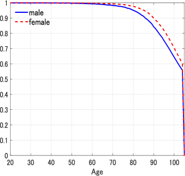
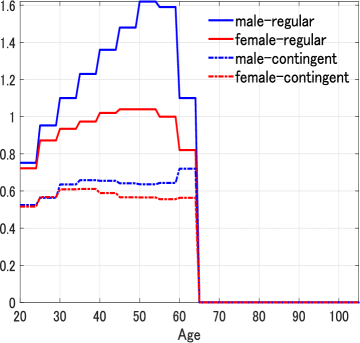
(a)  Survival rate                                   (b)  Labor productivity

Figure 6: Survival rate and labor productivity

We use the per capita medical and LTC expenditures presented by Iwamoto and Fukui (2018). The expected medical expenditure $m_{j,t}^{H}$ is obtained by multiplying the gender-specific survival rates presented in Figure 6 Panel (a) and the per capita age-specific expenditure data shown in Figure 5. Furthermore, the expected LTC expenditures $m_{j,t}^{L}$ is obtained by multiplying the gender-specific survival rates, the certification rate of LTC need, and the per capita age-specific expenditure data mentioned above. Figure 7 Panel (a) and (b) show the expected medical and LTC expenditures per capita, respectively. Because the survival rates are higher for females than for males, especially for those aged 60 and older, the expected medical and LTC expenditures are also higher for females.

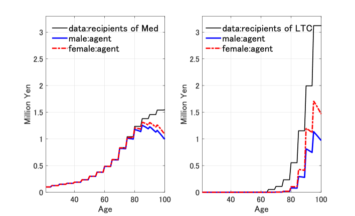
(a)  Medical expenditure             (b)  LTC expenditure

Figure 7: Expected medical and LTC expenditure (per capita)

4.3 Preferences

As shown in equation (22), an agent’s utility function is composed of consumption and labor supply, and, while the log function is used for consumption, the CES function is adopted for the disutility of labor. Kuroda and Yamamoto (2008) estimated the value of Frisch labor supply elasticity $\zeta^{g}$ ($g\in\{m,f\}$; hereafter Frisch elasticity), which differs between males and females, using data in Japan. Therefore, we conduct our analysis based on their estimation results. The Frisch elasticity in gender units is set as $\zeta^{m}=0.03$ for males, and $\zeta^{f}=0.05$ for females, and the preference parameter of leisure $\gamma=10$ for both males and females.

$$u_{i}(c_{t},l_{t})=\text{log}(c_{t})+\gamma\,\frac{(1-l_{t})^{1-\zeta^{g}}}{1-\zeta^{g}}.$$ (22)

The labor supply in the initial steady state of the four heterogeneous agents calculated using the parameters described above is shown in Figure 8 Panel (a). As can be seen in this figure, regardless of the age, labor income, gender, or employment type of the worker, agents spent around eight hours a day (about one-third of a day) working. In addition, the labor supply is higher for males than for females. These are consistent with the results of empirical studies such as the one Kuroda and Yamamoto (2008).

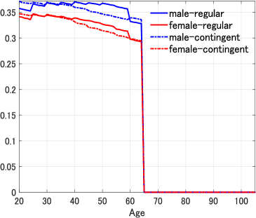
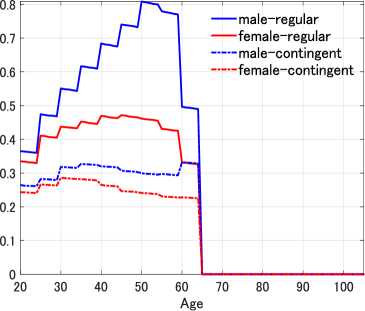
(a)  Labor supply                                   (b)  Labor income

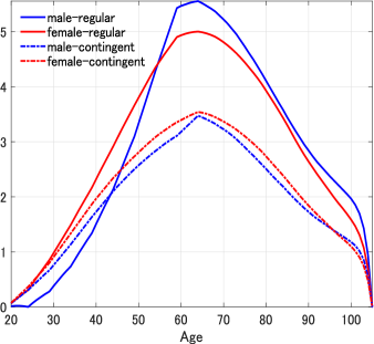
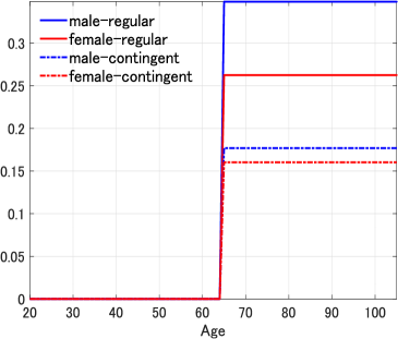
(c)  Assets                                               (d)  Pensions

Figure 8: Distribution of individual variables in the initial steady state

4.4 Technology

The technology parameters in Table 3 govern the technology growth rate ($\gamma_{A}=0.3\%$), investment rate, and capital income share in both sectors. The long-run growth rate for labor-augmented technology $\gamma_{\Omega}$ is set at 0.7%. By combining the two technology growth rates with the long-run population growth rate $\gamma_{n}$ indicating the demographic parameters as $-1.0$%, then the long-run GDP growth rate is offset as just 0%.

In Table 3, the share parameter of the aggregate production function, equation (10) $\eta_{1}$ (which determines the relative share of income for Sector 1) is set to 64%. This parameter is based on the share of operating surplus and mixed income in Sector 1. Following McGrattan et al. (2018), we use the JSNA data (average from 2015 to 2019) to determine the relative amounts of investment and fixed assets in the two sectors of production. Thus, by choosing the tangible capital ratio ($\theta_{1T}$, $\theta_{2T}$) and the tangible depreciation rate ($\delta_{1T}$, $\delta_{2T}$), we can ensure that the model’s investment and fixed assets are consistent with the JSNA’s tangible investment and equity (see table 2). Accordingly, the tangible capital shares of the two sectors are calibrated as $\theta_{1T}=0.45$ and $\theta_{2T}=0.35$. The annual depreciation rates that produce investment rates consistent with the Japanese data are $\delta_{1T}=0.08$ and $\delta_{2T}=0.05$. The tangible capital share and depreciation rate in Sector 2 include housing costs for the household business sector. The intangible capital ratio and depreciation rates, $\theta_{1I}$, $\theta_{2I}$, $\delta_{1I}$, and $\delta_{2I}$, cannot be identified uniquely with the data that we have. In our baseline model, we calibrated these parameters following Arato and Yamada (2012) who derived estimates of tangible and intangible assets for Sector 1. To calibrate the intangible assets in Sector 2, we suppose the same ratio of intangible assets and non-land fixed assets. As a result, we set these parameters to $\theta_{1I}=0.15$, $\theta_{2I}=0.05$, $\delta_{1I}=0.08$, and $\delta_{2I}=0.09$.

Table 3: Parameters of the model economy calibrated to Japan’s data

Parameters	Descriptions	Values
$\gamma^{n}$	Growth rate of the population (long-run)	$-1\%$
$J^{R}$	Retirement age	46
$J$	Maximum possible age	101
Preference parameters
$\gamma$	Preference parameter of leisure	10.0
$\zeta^{m}$	Frisch elasticity for male	0.03
$\zeta^{f}$	Frisch elasticity for female	0.05
$\beta$	Discount factor	0.983
Technology parameters
$\gamma^{A}$	TFP growth rate	0.3%
$\gamma^{\Omega}$	Labor-augmented productivity growth rate	0.7%
$\eta_{1}$	Income share of corporate sector	0.640
Interest rate of bond
$i_{t}^{d}$	Interest rate on government bonds	0.01
Capital shares
$\theta_{1T}$	Tangible capital of corporate sector	0.450
$\theta_{1I}$	Intangible capital of corporate sector	0.150
$\theta_{2T}$	Tangible capital of household business	0.350
$\theta_{2I}$	Intangible capital of household business	0.050
Depreciation rates
$\delta_{1T}$	Tangible capital of corporate sector	0.080
$\delta_{1I}$	Intangible capital of corporate sector	0.080
$\delta_{2T}$	Tangible capital of household business	0.050
$\delta_{2I}$	Intangible capital of household business	0.090
Fiscal policy parameters
$\psi_{G}$	Government consumption	0.190
$\psi_{B}$	Government debt	1.500
Capital tax rates
$\tau_{1}^{\pi}$	Corporate income tax	0.250
$\tau_{1}^{d}$	Tax on corporate distributions	0.250
$\tau_{2}^{d}$	Tax on household business distributions	0.250

1. The set values of parameters other than the preference parameters rely on the values from McGrattan et al. (2018). The values of the labor supply parameters are derived from the estimation of the labor supply elasticity of Kuroda and Yamamoto (2008).

4.5 Employment, labor income, and assets

In our model, $e^{j,g,h}$ represents the efficiency units supplied to the labor market by a group of agents of age $j$, gender $g$, and employment type $h$. To establish the labor productivity of the four types, that is, combinations of male or female and regular workers or contingent workers, we calculate the hourly wages for each type of worker. This result is shown in Figure 6 Panel (b). For data on wages and working hours, we use the Basic Survey on Wage Structure Statistics (2019). Using these data, we calculate hourly wages for each male and female, regular and contingent worker, and then we estimate labor productivity based on the method presented by Hansen (1993) and used by Braun et al. (2006), Yamada (2011), and others. Figure 8 Panel (b) shows the age distribution of labor income calculated in the initial steady state based on this labor productivity. In our analysis, since the baseline retirement age is set uniformly at 65, labor productivity is set so that it will reach zero at age 65. For both male and female regular workers, the hourly wages and labor productivity decline sharply after reaching the age of 60, but this is thought to reflect the decline in wages due to reemployment after the retirement age of 60, which is actually adopted by most companies.

The distribution of assets for each agent in the initial steady state is shown in Figure 8 Panel (c). This distribution indicates that male regular workers accumulate fewer assets at a younger age than female regular workers and that they begin to increase them rapidly after the age of 40. After the age of 50, the assets of male regular workers are lager than those of female regular workers. The reason for this lies in the shape of the labor productivity curve shown in Figure 6 (b) and the labor income shown in Figure 8 Panel (b). That is, the productivity and income of male regular workers increase significantly by the peak in their early 50s compared with female regular workers. Male regular workers are aware of this and thus are able to allocate a larger share of their income to consumption in their younger years.

4.6 Government

Social security system and fiscal balance

The government runs a PAYG pension system. In the baseline simulation, the normal retirement age $J^{R}$, equivalent to age 65, is set at 46. As shown in Figure 8 Panel (d), pension payments are calculated from an income replacement rate of 62%. Medical and LTC costs per capita are based on the amounts published in the Basic Data on Medical Insurance and the Statistics of Long-Term Care Benefit Expenditures by the Ministry of Health, Labour and Welfare, and are calculated following Iwamoto and Fukui (2018). In our quantitative analysis, we set the upper limit of the government debt-to-GDP ratio at 1.5 in the steady state. In addition, we suppose that the fiscal balance is adjusted by changes in the consumption tax during the transition path.

Tax system

Progressive taxation is set according to the income bracket of the household. McGrattan et al. (2018) use income and promotion tax tables estimated by IMF staff using National Tax Agency data. In our study, we also use the tax rates per income bracket they estimated. The details are shown in Table 4. Here, we suppose that the progressive labor tax of our model consists mainly of national and local taxes, such as inhabitant taxes, public pension, public medical insurance, and LTC insurance premiums.

Table 4: Progressive tax table for labor tax

Labor earnings	Share	Tax rate	$\alpha$	$\beta$
Under 1	17.3	0.027	0	0
1–2	15.0	0.191	$-0.0164$	0.0027
2–3	15.5	0.272	$-0.0326$	0.0218
3–4	15.4	0.285	$-0.0365$	0.049
4–5	12.2	0.294	$-0.0401$	0.0775
5–6	8.3	0.302	$-0.0441$	0.1069
6–7	5.1	0.306	$-0.0465$	0.1371
7–8	3.5	0.315	$-0.0528$	0.1677
8–9	2.4	0.324	$-0.0600$	0.1992
9–10	1.5	0.328	$-0.0636$	0.2316
10–15	2.8	0.338	$-0.0736$	0.2644
15–20	0.6	0.358	$-0.1036$	0.4334
20–25	0.2	0.387	$-0.1616$	0.6124
Over 25	0.2	0.447	$-0.3116$	0.8059
Total	100.0

1. Following McGrattan et al. (2018), the second column "Share" is obtained from the distribution of labor income based on the Tax Surveys published by the National Tax Agency. The third column "Tax rate" also contains the estimates of effective income tax rates across 14 income brackets obtained from McGrattan et al. (2018). The fourth and fifth columns "$\alpha$" and "$\beta$", which are calculated from the tax rate, are referred to as the intercept and slope of the progressive tax structure, respectively.

The capital tax rates are shown in Table 3. The effective corporate income tax rate $\tau_{1}^{\pi}$ is set at 25% to bring the modeled values in line with the corporate income tax and other corporate taxes paid by corporations in the JSNA. In addition, investors in corporations in which distributions are paid in the form of dividends will pay an additional tax on distributions. These tax rates $\tau_{1}^{d},\tau_{2}^{d}$ are set at 25 % to match the capital income and the size of the corporate sector.

Table 3 also contains the fiscal policy parameters. $\psi_{B}$ is defined as the total debt of the general government minus the financial assets held by public pension funds. These assets are accumulated for future pension liabilities, and we also incorporate them into our model. The level of government consumption $\psi_{G}$ is set to a constant percentage of adjusted GDP over the entire period.

5 Numerical analysis

In this section, we describe the quantitative results of a policy simulation for the transition path. Our simulation is based on two scenarios: (i) the baseline and (ii) the extension of the retirement age. For these two scenarios, we conduct policy simulations for the three options of social security reforms described below. Then, we calculate the impact on the current working, retired, and future generations for the four types of households distinguished by gender and employment type, and evaluate the extent to which differences in the impact are generated for the four types.

We proceed with the following three aspects. First, we outline the economic circumstances underlying the two scenarios and the three options of social security reforms. Second, we show how the transition paths of key aggregate economic variables would change if one of the three reforms is implemented in the two scenarios. In particular, we focus on changes in the real GDP and the level of the consumption tax rate. Third, we compare the impacts of the different reforms on the welfare for the current working, retired, and future generations. We then discuss the effects of the reforms, focusing on the inter-generation and intra-generation heterogeneity of households.

5.1 Scenarios and social security reforms

Here, we describe the two scenarios and three social security reforms in our analysis. As mentioned in section 4, we suppose that (i) the TFP growth rate $\gamma_{A}$ is 0.3%, the long-run labor-augmented technology growth rate $\gamma_{\Omega}$ is 0.7%, the retirement age $J^{R}$ is 46 (the age of 65), and the long-run population growth rate $\gamma_{n}$ is $-1$% in the baseline scenario. In the extended retirement age scenario, (ii) the only change from the baseline is that the retirement age $J^{R}$ increases from 65 to 70 in 2030.

In these two scenarios, we conduct policy simulations in the cases of the three reforms and the cases in which reforms are not implemented. That is, (1) continuation of the current policy, (2) a gradual decrease of the pension income replacement rate $\kappa_{t}$, (3) an increase in the copayment rate $\lambda_{j,t}^{H}$ for medical expenditures, and (4) an increase in the copayment rate $\lambda_{j,t}^{L}$ for LTC expenditures. In policy (1), we suppose that the pension income replacement rate $\kappa_{t}$ is constant at 62% and the copayment rate for medical expenditures $\lambda_{j,t}^{H}$ is 30% for those aged 20 to 70, 20% for those aged 70 to 75, 10% for those aged 75 and over, and 10% for LTC expenditures $\lambda_{j,t}^{L}$. Policy (2) is a reform to reduce the pension income replacement rate from 62% as of 2015 to 50.8% in 2047. Policy (3) is a reform to raise the copayment rate for health care expenditures for the elderly in 2030 to a uniform 30% for all ages. Policy (4) is a reform that would set the copayment rate for LTC expenditures at 30% in 2030.

5.2 Transition of aggregate variables

Here, we present the simulation results for the transition path of the real GDP, its growth rates, and the consumption tax rates under the demographic projection in which the population growth rates that are adopted are those of the IPSS (2017) up to 2115, and they are reduced by 1 % per year after 2115. The proportions of regular workers and contingent workers are supposed to be constant on the Basic Survey of Wage Structure Statistics in 2019 over the future.

5.2.1 Transition of the output

First, we focus on the transition path of the output. Figure 9 Panel (a) shows the transition of the level of the real GDP, normalized to unity for the year 2020 in the baseline scenario. Although GDP growth is downward until the mid-2050s, when the aging of the population will be at its peak, we see a gradual increase in GDP growth after around 2050.

Figure 9 Panel (b) shows the values of the comparisons by percentages of the level of the real GDP for each reform of both scenarios relative to the continuation of the current policy of the baseline scenario. As shown in the legend in the graph, the blue, red, or green dashed line represents the reduction in the pension replacement rate (RR 50%), a decreasing copayment for medical expenditures (Med 30%), or a decreasing copayment for LTC expenditures (LTC 30%), in the baseline scenario, respectively. Similarly the blue, red, or green solid line represents RR 50%, Med 30%, or LTC 30% in the extended retirement scenario ( [RE] ). In all cases of reforms in the two scenarios, the level of GDP is higher than the case of no reform in the baseline scenario for all periods. The reform of increasing copayments for medical and LTC expenditures in the baseline (the red dashed line and green dashed line) is at most a 1% increase. However, it increases to about 2.5% in the case of reducing the pension income replacement rate (the blue dashed line).

In the extended retirement scenario, the difference between the policies is even larger. The blue solid line shows an increase to just under 4% in the case of a reduction of the pension income replacement rate. This result shows that the level of GDP transition in the future is highest when the retirement age is extended and the reduction of the pension income replacement rate is introduced.

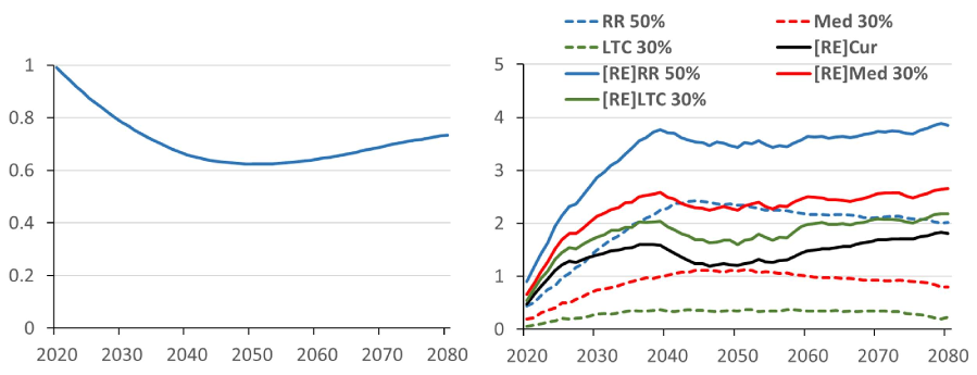
(a)  Transition of the GDP           (b)  Percentage change of the GDP induced by each reform

Figure 9: Transition of the real GDP and percentage change induced by each reforms

1. [RE] indicates the extended retirement scenario.

Figure 10 shows the growth rates of output in the baseline scenario, and the contribution decomposition of factors including intangible assets. Based on the production function described in section 3, the growth rate of output is decomposed into TFP $A_{t}$, tangible assets $K_{iT}$ in sector $i$, intangible assets $K_{iI}$, the labor force $L_{i}$ in sector $i$, and the population growth.

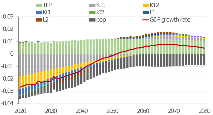
Figure 10: Output growth rate and its contribution decomposition

The total of the TFP growth rate and the labor-augmented technology growth rate (the light green bars) is stable at about 1% for the contribution, following our setting. In contrast, the growth rate of the population (dark gray bars) is shown as $-1$% for the contribution. These two contributions are approximately offset to 0% growth. On the other hand, a major factor depressing the growth rate of output through 2050 is the growth rate of tangible assets in Sector 1 (light gray bars) and tangible assets in Sector 2 (yellow bars).

This is due to both a decrease in the labor force population and an increase in the retired population making the aggregate saving rate, or capital accumulation drop rapidly in this period. Our simulations show that the size of the negative contribution of tangible and intangible assets to the output is much larger than that of the negative contribution of the labor force shown by the blue and brown bars.

5.2.2 Transition of the consumption tax rate

Next, we turn to the consumption tax rates. These transition paths are shown in Figure 11, where the consumption tax rates raises to around 42–43% at the peak in the mid-2050s in both scenarios if the current policy is maintained. Previous studies such as Braun and Joines (2015), have also shown generally consistent trends, albeit with differences in population growth rates and policy simulation assumptions.

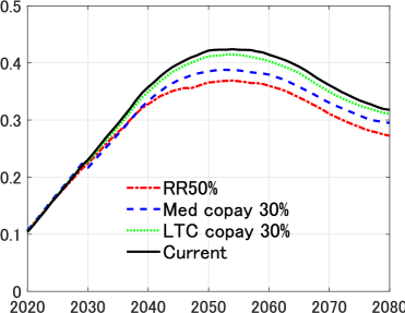
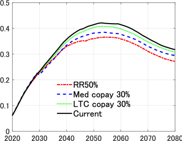
(a) Baseline                                   (d) Retirement extension

Figure 11: Transition path of consumption tax

The impact of the reforms on the consumption tax rate can be summarized as the following three points. First, all reforms would also reduce the peak level and lower the tax rate in the long-run compared with the current policy. Second, among the three reforms, the effect of reducing the pension replacement rate would be the largest, reducing the tax rates to about 36% in the mid-2050s in both scenarios. Third, the effect of rising the copayment rates for medical and LTC expenditures is smaller than the effect of reducing the pension income replacement rate. In addition, the effect in the case of increasing the copayments for LTC expenditures is even smaller, falling to about 38–39% in the mid-2050s in the case of health care and to about 41–42 % in the mid-2050s in the case of LTC expenditures in both scenarios.

5.3 Welfare analysis

Using the no-reform case as a benchmark, we assess the impact on the welfare of the three social security reforms for all generations, distinguishing the current working, the current retired, and the future generations in the two scenarios. We also consider the heterogeneity of the four types of households, distinguished by gender and employment type.

First, let us deal with the reform involving a reduction in the pension income replacement rate. This reform results in a significant fall in the welfare of individuals around retirement age in the present in both scenarios (Figure 12 Panel (a) and (b)). We consider the impact to be that individuals in this age group, who have already paid most of their pension contributions, will begin to receive pension benefits when the benefit is reducing. In the baseline scenario, welfare declines for almost all ages of the current retired and working generations, although in the extended retirement scenario, each type of agent’s welfare improves by about 2–5% for the working generation. This pension reform also causes a more significant decline in benefits for regular workers than for contingent workers for both the male and the female group. As discussed in section 4, we deduce that the reason for this is that regular workers, who have relatively higher incomes, pay more in pension contributions, despite receiving reduced benefits.

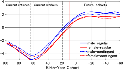
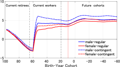
(a) Baseline                                      (d) Retirement extension

Figure 12: Welfare change due to replacement rate reduction

• The vertical red line drawn from 10 on the x-axis indicates the year in which the medical and LTC reforms will take place. The figure shows the percentage change in welfare relative to the current policy.

Next, we move on to the reform rising the copayment rate in the medical insurance. Figure 13 Panel (a) shows a similar trend to the pension reform in the baseline scenario. In particular, there is a significant decline in the welfare of the current retirees. The reform also shows a substantial decrease in welfare for both male and female contingent workers. For instance, the welfare of female contingent workers declines by at most 4%. In the extended retirement scenario, similar to the pension reform, the welfare of the current working-age population improves (Figure 13 Panel (b)).

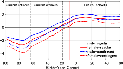
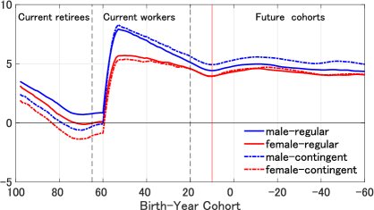
(a) Baseline                                      (d) Retirement extension

Figure 13: Welfare change due to medical copayment up to 30%

• The vertical red line drawn from 10 on the x-axis indicates the year in which the medical and LTC reforms will take place. The figure shows the percentage change in welfare relative to the current policy.

Finally, we describe the reform increasing the copayment rate of LTC insurance. In the baseline scenario, Figure 14 Panel (a) shows a decline in welfare for the current older age groups compared with the medical care case. This result is consistent with the LTC expenditures being higher per capita expenditures for those aged 90 and older compared with health care, as discussed in section 4. The extended retirement age scenario shows a similar trend to the medical insurance reform (Figure 14 Panel (b)).

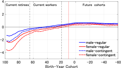
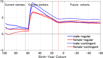
(a) Baseline                                      (d) Retirement extension

Figure 14: Welfare change due to LTC copayment up to 30%

• The vertical red line drawn from 10 on the x-axis indicates the year in which the medical and LTC reforms will take place. The figure shows the percentage change in welfare relative to the current policy.

The size of the changes in welfare based on the three reforms ("RR50", "Med10", "LTC10") compared to the current system is summarized in Table 5. The item for "Total" is the size of the change in welfare aggregated across the three generations over the entire period, while the items for "Retire", "Worker", and "Future" are those for each of the generations. Positive values of item "Future" in the table indicates that all three reforms increase the welfare of all four agents of future generations, while negative values of "Retiree" and "Worker" show they decline the welfare of all four agents of the current retired and working generations in the baseline scenario. In particular, the average welfare drop of female contingent workers in the medical and LTC reforms is significant, amounting to minus 2.3–3.4 percent. However, these reforms in the extension of the retirement age scenario eliminate the decrease in welfare of current generations. Indeed, there are all positive values for all agents except a few of item "Retire" in the columns of "Extension of Retirement Age" in the table.

Table 5: Summary of welfare analysis

		1. Baseline				2. Extension of Retirement Age
		Total	Retire	Worker	Future	Total	Retire	Worker	Future
RR50	male-regular	$-$0.325	$-$3.666	$-$2.857	2.008	3.555	$-$0.129	3.259	4.993
	female-regular	$-$0.787	$-$3.707	$-$3.344	1.408	2.921	$-$0.234	2.090	4.414
	male-contingent	$-$0.304	$-$3.195	$-$2.601	1.762	4.434	0.287	4.506	5.867
	female-contingent	$-$0.751	$-$3.408	$-$3.137	1.273	3.420	0.000	2.830	4.897
Med10	male-regular	0.554	$-$1.741	$-$0.184	1.700	4.355	1.776	5.910	4.561
	female-regular	0.037	$-$2.348	$-$0.807	1.263	3.665	1.081	4.600	4.154
	male-contingent	$-$0.137	$-$2.852	$-$0.930	1.184	4.485	0.538	6.105	5.144
	female-contingent	$-$0.688	$-$3.426	$-$1.631	0.709	3.402	$-$0.123	4.283	4.248
LTC10	male-regular	0.192	$-$0.799	0.075	0.597	3.992	2.455	6.114	3.571
	female-regular	$-$0.131	$-$1.589	$-$0.227	0.428	3.421	1.429	5.058	3.382
	male-contingent	$-$0.001	$-$1.308	$-$0.061	0.489	4.555	1.680	6.899	4.506
	female-contingent	$-$0.426	$-$2.358	$-$0.463	0.274	3.501	0.386	5.269	3.798

• The item for "Total" is the size of the change in welfare aggregated across the three generations over the entire period, while the items for "Retiree", "Worker", and "Future" are those for each of the generations.

5.4 Discussion

Here, we pay more attention to the following three aspects based on our simulation results. First, we find that real GDP growth would decline with aging until the mid-21st century and that most of the decline appears to be attributable to the fall in the capital stock rather than to the decline in the labor force (Figure 10). Second, our welfare analysis shows that social security reform has a low impact on the welfare of the current generation in our baseline scenario. However, the magnitude of the impact varies by household type. Pension reform lowers the welfare of regular workers by about 4%, while it lowers the welfare of contingent workers by about 1%. In other words, the negative impact is more significant for regular workers. Medical and LTC reform lowers the welfare of women and contingent workers by about 2 to 3%, while it lowers the welfare of male regular workers by about 1%. In other words, the negative impact is more significant for women and contingent workers. Third, extending the retirement age at the same time as social security reform would mitigate the current generation’s decline in welfare by about 3 to 4%.

These counterfactual simulations suggest that extending the retirement age combined with social security reform is necessary to mitigate the decrease in the welfare of the current generation. Our simulations also show that social security reform lowers the welfare of the current generations, with a more negative impact on the lower-income segments (women and contingent workers).

Why, then, does the pension reform reduce the welfare of regular workers to a relatively large extent, while medical and LTC reform reduce the welfare of households belonging to lower income group to a large extent? One of the most significant reasons is that pension benefits depend on labor income during the working age. Regular workers with relatively higher incomes are likely to experience a decline in welfare because of the significant decrease in benefits due to the reduction in the pension income replacement rate. In our calculations, on the other hand, we suppose that medical and LTC expenditures are independent of income and arise depending on age and gender differences. Therefore, we suppose that the medical and LTC reforms led to a decline in welfare for households with lower income types.

Health and income risks in old age affect behavior in younger age. Braun et al. (2017) pointed out that, given the various risks in old age, increasing social security benefits by expanding means-tested social insurance improves welfare. Meanwhile, in our simulations, social security reform significantly lowers welfare for households with relatively low incomes and whose incomes do not increase with age. Our simulations could be consistent with theirs in this regard. Therefore, when reforming social security, it is necessary to mitigate the decline in welfare by redistributing benefits to low-income groups such as females and contingent workers.

However, our study would have the following challenges. Our model supposes single households for all types of gender and employment types. However, as summarized in Doepke and Tertilt (2016), recent studies have used models with married couples or children in the household and have considered the insurance effect among family members against various shocks (e.g., Blundell et al., 2018; Fernández and Wong, 2014; Kitao and Mikoshiba, 2022). For example, if a woman has a low income, but her spouse has a high income, her decision-making will naturally differ from that of a single woman. Therefore, we suppose that family functioning plays an essential role in considering social security reform’s impact in more detail.

6 Conclusion

This paper quantitatively explores the impact of pension, medical, and LTC insurance reforms on households’ welfare in Japan, where the population is aging remarkably, through policy simulations using an OLG model with four types of households distinguished by gender and employment type.

Our simulations show that all three options of social security reforms raise the welfare of future generations, in contrast to having a significantly negative impact on low-income groups, females and contingent workers, in the current generations. We also find that these reforms affect females negatively. However, combining the extension of the retirement age with social security reforms mitigates the negative impact on the current generations’ welfare by 3 to 4%. The result suggests that the negative impact of social security reforms on welfare could be reduced by paying enough attention to the impact on females and contingent workers, who are relatively vulnerable groups.

However, there are the following challenges in our study. Firstly, since future medical and LTC expenditures depend on uncertainty, such as individual health status, there are many implications of focusing on future uncertainty, especially in the context of the retirement saving puzzle, for which the literature has recently accumulated (e.g., De Nardi et al., 2010; Kopecky and Koreshkova, 2014). In contrast, our model is that households behave deterministically. The next challenge is that our model omits the effect of risk sharing on future uncertain spending among married couples. As mentioned in the previous section, some recent research focuses on such family effects, and Braun et al. (2017) quantifies the risk of becoming single after retirement.

Analyzing such effects more rigorously requires microdata on such ad household consumption, income, medical, and LTC expenditures. Our analysis, however, is based on aggregate data. We may be able to provide more practical and meaningful policy implications for social security reforms while mitigating negative impacts as much as possible by overcoming these challenges. We want to make these challenges our next research subject.

References

- (1)
- Arato and Yamada (2012) Arato, Hiroki and Katsunori Yamada (2012) “Japan’s intangible capital and valuation of corporations in a neoclassical framework,” Review of Economic Dynamics, 15 (4), 459–478.
- Blundell et al. (2018) Blundell, Richard, Luigi Pistaferri, and Itay Saporta-Eksten (2018) “Children, Time Allocation, and Consumption Insurance,” Journal of Political Economy, 126 (S1), S73–S115.
- Braun et al. (2006) Braun, R. Anton, Daisuke Ikeda, and Douglas H. Joines (2006) “Saving and Interest Rates in Japan: Why They Have Fallen and Why They Will Remain Low,” Federal Reserve Bank of San Francisco, Working Paper Series, 1–33.
- Braun and Joines (2015) Braun, R. Anton and Douglas H. Joines (2015) “The implications of a graying Japan for government policy,” Journal of Economic Dynamics and Control, 57, 1–23.
- Braun et al. (2017) Braun, R. Anton, Karen A. Kopecky, and Tatyana Koreshkova (2017) “Old, Sick, Alone, and Poor: A Welfare Analysis of Old-Age Social Insurance Programmes,” The Review of Economic Studies, 84 (2), 580–612.
- De Nardi et al. (2010) De Nardi, Mariacristina, Eric French, and John B Jones (2010) “Why Do the Elderly Save ? The Role of Medical Expenses,” Journal oc Political Economy, 118 (1), 39–75.
- Doepke and Tertilt (2016) Doepke, Matthias and Michèle Tertilt (2016) “Families in macroeconomics,” in Handbook of macroeconomics, 2, 1789–1891: Elsevier.
- Fernández and Wong (2014) Fernández, Raquel and Joyce Cheng Wong (2014) “Divorce Risk, Wages and Working Wives: A Quantitative Life-Cycle Analysis of Female Labour Force Participation,” Economic Journal, 124 (576), 319–358.
- Fu et al. (2017) Fu, Rong, Haruko Noguchi, Akira Kawamura, Hideto Takahashi, and Nanako Tamiya (2017) “Spillover effect of Japanese long-term care insurance as an employment promotion policy for family caregivers,” Journal of Health Economics, 56, 103–112.
- Hansen (1993) Hansen, Gary D. (1993) “The cyclical and secular behaviour of the labour input: Comparing efficiency units and hours worked,” Journal of Applied Econometrics, 8 (1), 71–80.
- Hansen and ImrohoroÄlu (2016) Hansen, Gary D. and Selahattin ImrohoroÄlu (2016) “Fiscal reform and government debt in Japan: A neoclassical perspective,” Review of Economic Dynamics, 21, 201–224.
- ImrohoroÄlu et al. (2017) ImrohoroÄlu, Selahattin, Sagiri Kitao, and Tomoaki Yamada (2017) “Can Guest Workers Solve Japan’S Fiscal Problems?,” Economic Inquiry, 55 (3), 1287–1307.
- ImrohoroÄlu et al. (2019) (2019) “Fiscal sustainability in Japan: What to tackle?,” Journal of the Economics of Ageing, 14.
- Iwamoto and Fukui (2018) Iwamoto, Yasushi and Tadashi Fukui (2018) “The model of Financing Medical and long-term care insurance (March 2018 version) ,” Working Paper (in Japanese).
- Kitao (2015) Kitao, Sagiri (2015) “Fiscal cost of demographic transition in Japan,” Journal of Economic Dynamics and Control, 54, 37–58.
- Kitao (2018) (2018) “Policy uncertainty and cost of delaying reform: The case of aging Japan,” Review of Economic Dynamics, 27, 81–100.
- Kitao and Mikoshiba (2020) Kitao, Sagiri and Minamo Mikoshiba (2020) “Why Women Work the Way They Do in Japan: Roles of Fiscal Policies,” Journal of the Japanese and International Economies, 56.
- Kitao and Mikoshiba (2022) (2022) “Females, the Elderly, and also Males: Demographic Aging and Macroeconomy in Japan,” Working paper.
- Kopecky and Koreshkova (2014) Kopecky, Karen A. and Tatyana Koreshkova (2014) “The impact of medical and nursing home expenses on savings,” American Economic Journal: Macroeconomics, 6 (3), 29–72.
- Kuroda and Yamamoto (2008) Kuroda, Sachiko and Isamu Yamamoto (2008) “Estimating Frisch labor supply elasticity in Japan,” Journal of the Japanese and International Economies, 22 (4), 566–585.
- McGrattan et al. (2018) McGrattan, Ellen, Kazuaki Miyachi, and Adrian Peralta-Alva (2018) “On Financing Retirement, Health, and Long-term Care in Japan,” IMF Working Papers, 18 (249), 1.
- McGrattan (2020) McGrattan, Ellen R. (2020) “Intangible Capital and Measured Productivity,” Review of Economic Dynamics, 37, S147–S166.
- McGrattan and Prescott (2017) McGrattan, Ellen R. and Edward C. Prescott (2017) “On financing retirement with an aging population,” Quantitative Economics, 8 (1), 75–115.
- McGrattan and Prescott (2018) (2018) “An Aggregate Model for Policy Analysis with Demographic Change,” Journal of the Economics of Ageing, 11, 52–61.
- Moriguchi (2017) Moriguchi, Chiaki (2017) “Did Japan Become an Unequal Society ?: Japan’s Income Disparity in Comparative Historical Perspective,” Economic Review, Hitotsubashi University, 68 (2), 169–189.
- Mukoyama et al. (2021) Mukoyama, Toshihiko, Mototsugu Shintani, and Kazuhiro Teramoto (2021) “Cyclical Part-Time Employment in an Estimated New Keynesian Model with Search Frictions,” Journal of Money, Credit and Banking, 53 (8), 1929–1968.
- Yamada (2011) Yamada, Tomoaki (2011) “A politically feasible social security reform with a two-tier structure,” Journal of the Japanese and International Economies, 25 (3), 199–224.
- Yamaguchi (2019) Yamaguchi, Shintaro (2019) “Effects of Parental Leave Policies on Female Career and Fertility Choices,” Quantitative Economics, 10 (3), 1195–1232.