Interpretable sensitivity analysis for the Baron–Kenny approach to mediation with unmeasured confounding

Abstract

Mediation analysis assesses the extent to which the exposure affects the outcome indirectly through a mediator and the extent to which it operates directly through other pathways. As the most popular method in empirical mediation analysis, the Baron–Kenny approach estimates the indirect and direct effects of the exposure on the outcome based on linear structural equation models. However, when the exposure and the mediator are not randomized, the estimates may be biased due to unmeasured confounding among the exposure, mediator, and outcome. Building on Cinelli and Hazlett (2020), we derive general omitted-variable bias formulas in linear regressions with vector responses and regressors. We then use the formulas to develop a sensitivity analysis method for the Baron–Kenny approach to mediation in the presence of unmeasured confounding. To ensure interpretability, we express the sensitivity parameters to correspond to the natural factorization of the joint distribution of the direct acyclic graph for mediation analysis. They measure the partial correlation between the unmeasured confounder and the exposure, mediator, outcome, respectively. With the sensitivity parameters, we propose a novel measure called the “robustness value for mediation” or simply the “robustness value”, to assess the robustness of results based on the Baron–Kenny approach with respect to unmeasured confounding. Intuitively, the robustness value measures the minimum value of the maximum proportion of variability explained by the unmeasured confounding, for the exposure, mediator and outcome, to overturn the results of the point estimate or confidence interval for the direct and indirect effects. Importantly, we prove that all our sensitivity bounds are attainable and thus sharp.

Keywords: causal inference; Cochran’s formula; direct effect; indirect effect; omitted-variable bias; robustness value

Introduction

1.1 Baron–Kenny approach and unmeasured confounding

Researchers are often interested in the causal mechanism from an exposure to an outcome. Mediation analysis is a tool for quantifying the extent to which the exposure acts on the outcome indirectly through a mediator and the extent to which the exposure acts on the outcome directly through other pathways. That is, it estimates the indirect and direct effects of the exposure on the outcome. The Baron–Kenny approach to mediation (Baron and Kenny 1986) is the most popular approach for empirical mediation analysis, with more than one hundred thousand google scholar citations in total when we were preparing for this manuscript. It decomposes the total effect of the exposure on the outcome based on linear structural equation models. However, with non-randomized exposure or mediator, unmeasured confounding can bias the estimates of the indirect and direct effects. A central question is then to assess the sensitivity of the estimates with respect to unmeasured confounding. This is often called sensitivity analysis in causal inference (e.g., Cornfield et al. 1959; Rosenbaum and Rubin 1983; Lin et al. 1998; Imbens 2003; Rothman et al. 2008; Ding and VanderWeele 2016).

Sensitivity analysis for mediation analysis has been an important research topic in recent years. Tchetgen and Shpitser (2012), Ding and Vanderweele (2016) and Smith and VanderWeele (2019) propose sensitivity analysis methods based on the counterfactual formulation of mediation analysis. They focus on nonlinear structural equation models. VanderWeele (2010) proposes a general formula for sensitivity analysis which can be used for the Baron–Kenny approach, and le Cessie (2016) also derives a formula for the Baron–Kenny approach. However, their resulting sensitivity parameters are not easy to interpret due to the unknown scale of the unmeasured confounding. Imai et al. (2010) propose a sensitivity analysis method for mediation analysis based on linear structural equation models. However, they do not discuss the most general form of the Baron–Kenny approach. Cox et al. (2013) compare and evaluate some existing methods for assessing sensitivity in mediation analysis.

It is still an open problem to develop an interpretable sensitivity analysis method for the most general form of the Baron–Kenny approach. It is perhaps a little surprising due to the popularity of the Baron–Kenny approach. A main challenge is to find parsimonious and interpretable sensitivity parameters that can quantify the strength of the unmeasured confounding with respect to the exposure, mediator and outcome. We fill this gap by leveraging the insight from a recent result in Cinelli and Hazlett (2020), with similar results also in Mauro (1990), Frank (2000) and Hosman et al. (2010). Their key idea is to use the partial $R^{2}$ as sensitivity parameters which measure the proportions of variability explained by unmeasured confounding conditional on the observed variables. The $R^{2}$ parameters are interpretable and bounded between $0$ and $1$. However, their formula cannot be applied immediately to sensitivity analysis for the Baron–Kenny approach, especially for the case with multiple mediators.

1.2 Our contributions

First, we derive a general omitted-variable bias formula, with vector responses and regressors and scalar unmeasured confounder, which extends Cinelli and Hazlett (2020). We propose a novel $R$ measure, and express the multivariate omitted-variable bias in terms of $R$ parameters. The $R^{2}$ parameters can be viewed as the Euclidean norm of the corresponding vector $R$ parameters, and thus our sensitivity parameters are bounded in a Euclidean unit ball. Our formula is based on the population least squares, and we suggest to use the nonparametric bootstrap to handle heteroskedasticity and more generally, model misspecification. The formula serves as the basis for the sensitivity analysis for the Baron–Kenny approach with possibly multiple mediators.

Second, we apply the formula to develop a sensitivity analysis method for the Baron–Kenny approach with a single unmeasured confounder. The main challenge is that a direct application of the omitted-variable bias formula depends on the sensitivity parameters not corresponding to the natural factorization of the directed acyclic graph for mediation analysis. This is also a challenge encountered by VanderWeele (2010) and Ding and Vanderweele (2016). They do not provide any solutions. We can solve the problem thanks to the properties of the $R$ parameters. Based on the $R$ parameters, we propose a novel measure and call it the “robustness value for mediation” or simply the “robustness value”. It is the minimum value of the maximum strength of these $R$ parameters measured by their Euclidean norms, or equivalently, their corresponding $R^{2}$ parameters, such that the point estimate can be reduced to $0$ or the confidence interval can be altered to cover $0$. Intuitively, the corresponding $R^{2}$ parameters can be interpreted as the proportions of variability explained by the unmeasured confounding in the exposure, mediator, and outcome models given the observed variables.

Third, we extend our sensitivity analysis method to allow for multiple unmeasured confounders. A common trick is to consider a linear combination of the unmeasured confounders from the least squares regression that could fully characterize the omitted-variable bias, and thus the problem reduces to the discussion with a single unmeasured confounder (Hosman et al. 2010; Cinelli and Hazlett 2022). Although this trick works well for many problems, it does not apply to sensitivity analysis for the indirect effect with multiple mediators. The trick of reducing multiple unmeasured confounders to a single confounder breaks down because the exposure could affect the outcome through the mediators in multiple paths, thus a single confounder could not characterize all the confounding in these paths. As a solution, we further derive and apply a general omitted-variable bias formula with vector responses, regressors, and unmeasured confounders. With the general formula, we provide solutions to compute the robustness values that allow for multiple unmeasured confounders. To the best of our knowledge, this has not been done before even for the simple least squares, let alone the more complicated mediation analysis.

Fourth, we show all our sensitivity analysis methods are sharp in the sense that given the observables, the sensitivity parameters can freely take arbitrary values in their feasible regions.

1.3 Notation and definitions

Let $\mathrm{dim}(\cdot)$ denote the dimension of a vector. For vector $x$, let $x_{j}$ denote the $j$th coordinate of $x$, and $x_{-j}$ denote the vector after removing the $j$th coordinate of $x$. Let $I$ denote the identity matrix with the dimension implicit and clear in the context. For positive semi-definite matrix $A$, let $A^{1/2}$ denote the symmetric square root of $A$.

Let $\|\cdot\|_{2}$ denote the Euclidean norm of a vector. We also use $\|\cdot\|_{2}$ to denote the matrix norm induced by the Euclidean norm, i.e., $\|A\|_{2}=\sup_{x\not=0}\|Ax\|_{2}/\|x\|_{2}$ for matrix $A$, which is also known as the spectral norm. When $A$ reduces to a vector, the spectral norm of $A$ is equal to the Euclidean norm of $A$. Let $\|\cdot\|_{\mathrm{F}}$ denote the Frobenius norm of a matrix. Let $\mathbb{B}_{d}$ denote the open unit ball of $d$-dimensional vectors with respect to the Euclidean norm, i.e., $\mathbb{B}_{d}=\{x\in\mathbb{R}^{d}:\|x\|_{2}<1\}$. Let $\partial\mathbb{B}_{d}$ denote the boundary of $d$-dimensional unit ball with respect to the Euclidean norm, i.e. $\partial\mathbb{B}_{d}=\{x\in\mathbb{R}^{d}:\|x\|_{2}=1\}$, and $\overline{\mathbb{B}}_{d}$ denote the closed $d$-dimensional unit ball with respect to the Euclidean norm, i.e. $\overline{\mathbb{B}}_{d}=\{x\in\mathbb{R}^{d}:\|x\|_{2}\leq 1\}$. Let $\mathbb{B}_{d_{1}\times d_{2}}$ denote the open unit ball of $d_{1}\times d_{2}$ matrices with respect to the spectral norm, i.e. $\mathbb{B}_{d_{1}\times d_{2}}=\{x\in\mathbb{R}^{d_{1}\times d_{2}}:\|x\|_{2}<1\}$. Let $\mathbb{S}_{n}^{++}$ denote the sets of $n\times n$ positive definite matrices.

Let $\mathrm{corr}(\cdot,\cdot)$ denote the correlation coefficient of two random variables. Let $\hat{\mathrm{var}}(\cdot)$ denote the sample variance of a vector, $\hat{\mathrm{cov}}(\cdot)$ denote the sample covariance matrix of a data matrix, and $\hat{\mathrm{corr}}(\cdot,\cdot)$ denote the sample correlation coefficient of two scalars. Let $\perp\!\!\!\!\perp$ denote independence of random variables.

We review the definition of least squares below. For least squares, we use lowercase letters to denote random variables, uppercase letters to denote the observed vectors or matrices for independent samples from the corresponding random variables, and Greek letters to denote the coefficients in regressions, respectively. We assume that all random vectors are column vectors and the coefficients from least squares are vectors or matrices with suitable dimensions.

Definition 1.

(i) For scalar $y$ and vector $x$, the population least squares regression of $y$ on $x$ is $y=\beta^{\mathrm{\scriptscriptstyle T}}x+y_{\perp x}$, where $\beta=\arg\min_{b}E\{(y-b^{\mathrm{\scriptscriptstyle T}}x)^{2}\}$, and $y_{\perp x}=y-\beta^{\mathrm{\scriptscriptstyle T}}x$ denotes the population residual. If $y$ is a vector, then $\beta$ is a matrix that minimizes $E\{\|y-b^{\mathrm{\scriptscriptstyle T}}x\|_{2}^{2}\}$.

(ii) For vector $Y$ and matrix $X$, the sample least squares regression of $Y$ on $X$ is $Y=X\hat{\beta}+Y_{\perp X}$, where $\hat{\beta}=\arg\min_{b}\|Y-Xb\|_{2}^{2}$, and $Y_{\perp X}=Y-X\hat{\beta}$ denotes the sample residual vector. If $Y$ is a matrix, then $\hat{\beta}$ is a matrix with each column corresponding to the sample least squares coefficient of the corresponding column of $Y$ on $X$.

Definition 1 above does not assume that the linear model is correct. It will be fundamental for our discussion below. We also review the definition of the population $R^{2}$ and population partial $R^{2}$ in Definition 2 below.

Definition 2.

For scalar $y$ and vectors $x$ and $z$, define the population $R^{2}$ of $y$ on $x$ as $R_{y\sim x}^{2}=1-\mathrm{var}(y_{\perp x})/\mathrm{var}(y)$ if $\mathrm{var}(y)\not=0$, and the population partial $R^{2}$ of $y$ on $x$ given $z$ as $R_{y\sim x\mid z}^{2}=1-\mathrm{var}(y_{\perp x,z})/\mathrm{var}(y_{\perp z})$ if $\mathrm{var}(y_{\perp z})\not=0$.

Omitted-variable bias in least squares

2.1 Review of the omitted-variable bias formula with the $R^{2}$ parameterization

Let $y$ denote the outcome, $a$ the exposure, $c$ the observed covariates including the constant $1$, and $u$ the unmeasured confounder. Assume $y,a,u$ are scalars, and $c$ can be a vector. Consider the long and short population least squares regressions with and without $u$:

$$\begin{split}y&=\gamma_{1}a+\gamma_{2}^{\mathrm{\scriptscriptstyle T}}c+\gamma_{3}u+y_{\perp a,c,u},\\ y&=\tilde{\gamma}_{1}a+\tilde{\gamma}_{2}^{\mathrm{\scriptscriptstyle T}}c+y_{\perp a,c}.\end{split}$$ (1)

The difference between the coefficients of $a$ in the long and short regressions in (1) equals

$$\tilde{\gamma}_{1}-\gamma_{1}=\gamma_{3}\cdot\rho_{1},$$ (2)

where $\rho_{1}$ is the coefficient of $a$ in the population least squares regression of $u$ on $(a,c)$. The result in (2) is called Cochran’s formula in statistics (Cochran 1938; Cox 2007) and the omitted-variable bias formula in econometrics (Angrist and Pischke 2008). It has a simple form and is useful for sensitivity analysis with respect to unmeasured confounding. VanderWeele (2010) derives a similar formula without the linear forms in (1). However, it can be difficult to interpret the regression coefficients $\gamma_{3}$ and $\rho_{1}$ in (2) because $u$ is unmeasured with unknown scale.

Cinelli and Hazlett (2020) propose a novel $R^{2}$ parametrization of the omitted-variable bias:

$$\tilde{\gamma}_{1}-\gamma_{1}=\mathrm{sgn}(\tilde{\gamma}_{1}-\gamma_{1})\left(\frac{R_{y\sim u\mid a,c}^{2}R_{a\sim u\mid c}^{2}}{1-R_{a\sim u\mid c}^{2}}\right)^{1/2}\left\{\frac{\mathrm{var}(y_{\perp a,c})}{\mathrm{var}(a_{\perp c})}\right\}^{1/2}.$$ (3)

The formula (3) states that the difference $\gamma_{1}-\tilde{\gamma}_{1}$ depends on three types of quantities. First, it depends on the variances of the residuals $\mathrm{var}(y_{\perp a,c})$ and $\mathrm{var}(a_{\perp c})$, which are determined by the moments of the observables. Second, it depends on two $R^{2}$ parameters: $R_{a\sim u\mid c}^{2}$ measures the confounder-exposure partial correlation given observed covariates $c$, and $R_{y\sim u\mid a,c}^{2}$ measures the confounder-outcome partial correlation given the exposure $a$ and observed covariates $c$. Third, it depends on the sign of the bias $\mathrm{sgn}(\tilde{\gamma}_{1}-\gamma_{1})$. Since $u$ is unobserved, the bias $\tilde{\gamma}_{1}-\gamma_{1}$ can be positive or negative. The formula (3) is more interpretable than (2). Even with unknown scale of $u$, the $R^{2}$ is bounded between $0$ and $1$, and measures the proportion of variability explained by $u$. Imbens (2003) and Blackwell (2014) also propose to use the $R^{2}$-type sensitivity parameters for other settings.

Their original strategy for sensitivity analysis is restrictive in our discussion. First, they focus on the sample least squares and use the $R^{2}$ parameters to express the classical standard errors under homoskedasticity. However, it is difficult to use the $R^{2}$ parameters to express the robust standard errors. The robust standard errors, also known as the sandwich standard errors, allow for heteroskedasticity and model misspecification and are commonly used in practice. Second, the formula (3) assumes $y$ and $a$ are scalars. It cannot be applied immediately to the sensitivity analysis for the Baron–Kenny approach with multiple mediators. We present the sensitivity analysis with a single mediator based on their original strategy and discuss its difficulties; see Section B of the Supplementary Material.

To overcome the restrictions, first, we focus on the population least squares and suggest the nonparametric bootstrap for the inference. Since population least squares regression does not assume that the linear model is correct, the nonparametric bootstrap provides a valid inference that allows for heteroskedasticity and model misspecification. Second, we extend the formula (3) with vectors $y$ and $a$ based on novel $R$ parameters, as introduced in the following Section 2.2.

2.2 The $R$ measure and its properties

We propose a novel $R$ measure for the correlation between two centered vectors, or for the partial correlation of two vectors after controlling for a third vector including the constant $1$. We give the formal definition of the $R$ measure in Definition 3 below.

Definition 3.

For centered vectors $y$ and $x$, define

$$R_{y\sim x}=\mathrm{cov}(y)^{-1/2}\mathrm{cov}(y,x)\mathrm{cov}(x)^{-1/2}$$

if $\mathrm{cov}(y)$ and $\mathrm{cov}(x)$ are invertible. For vectors $y,x,z$, where $z$ includes the constant $1$, define

$$R_{y\sim x\mid z}=\mathrm{cov}(y_{\perp z})^{-1/2}\mathrm{cov}(y_{\perp z},x_{\perp z})\mathrm{cov}(x_{\perp z})^{-1/2}$$

if $\mathrm{cov}(y_{\perp z})$ and $\mathrm{cov}(x_{\perp z})$ are invertible.

Consider the special case when $y$ and $x$ are scalars in Definition 3. Then, $R_{y\sim x}$ reduces to the population Pearson correlation coefficient of $y$ and $x$, and $R_{y\sim x\mid z}$ reduces to the population partial correlation coefficient of $y$ and $x$ after controlling for $z$. Moreover, the squared $R_{y\sim x}$ and $R_{y\sim x\mid z}$ in Definition 3 are $R_{y\sim x}^{2}$ and $R_{y\sim x\mid z}^{2}$ in Definition 2, respectively.

Cinelli and Hazlett (2020) also use the same notation $R$ for the partial correlation coefficient in their discussion, but our Definition 3 allows for vectors $y$ and $x$ as well. When $y$ and $x$ are vectors, $R_{y\sim x}$ or $R_{y\sim x\mid z}$ is a matrix with dimension $\mathrm{dim}(y)\times\mathrm{dim}(x)$, satisfying $R_{y\sim x}=R_{x\sim y}^{\mathrm{\scriptscriptstyle T}}$ and $R_{y\sim x\mid z}=R_{x\sim y\mid z}^{\mathrm{\scriptscriptstyle T}}$.

To unify the definition of $R_{y\sim x}$ and $R_{y\sim x\mid z}$ in Definition 3, we can write $R_{y\sim x\mid z}=R_{y_{\perp z}\sim x_{\perp z}}$, where $y_{\perp z}$ and $x_{\perp z}$ are centered vectors. Also, it is well known in linear regression that $R_{y\sim x\mid z}^{2}=R_{y_{\perp z}\sim x_{\perp z}}^{2}$, for $R^{2}$ and partial $R^{2}$ in Definition 2. Thus, we can focus on the discussion of the $R$ measure of two centered vectors and the population $R^{2}$. Lemma 1 states that the Euclidean norm or spectral norm of the $R$ measure in Definition 3 is related to the $R^{2}$ in Definition 2.

Lemma 1.

For centered scalar $y$ and centered vector $x$, we have $\|R_{y\sim x}^{\mathrm{\scriptscriptstyle T}}\|_{2}^{2}=R_{y\sim x}^{2}$, if $\mathrm{var}(y)\not=0$ and $\mathrm{cov}(x)$ is invertible. For centered vectors $y$ and $x$, $\|R_{y\sim x}\|_{2}^{2}$ is the maximum of $R_{\alpha^{\mathrm{\scriptscriptstyle T}}y\sim x}^{2}$ over all linear combinations $\alpha^{\mathrm{\scriptscriptstyle T}}y\not=0$, if $\mathrm{cov}(y)$ and $\mathrm{cov}(x)$ are invertible.

We make two remarks below to discuss connections between $R_{y\sim x}$ and the marginal correlation coefficients of $y$ and $x$, and the connections between $R_{y\sim x}$ and the canonical correlation coefficients between $y$ and $x$.

Remark 1 (Connections with marginal correlation coefficients).

Let $\rho_{yx}\in\mathbb{R}^{\mathrm{dim}(y)\times\mathrm{dim}(x)}$ denote the marginal correlation matrix of $y$ and $x$, with the $(i,j)$th element of $\rho_{yx}$ equal to the correlation of $y_{i}$ and $x_{j}$. We can write

$$\rho_{yx}=\mathrm{diag}\{\mathrm{cov}(y)\}^{-1/2}\mathrm{cov}(y,x)\mathrm{diag}\{\mathrm{cov}(x)\}^{-1/2},$$

where $\mathrm{diag}(\cdot)$ is the diagonal matrix of a square matrix. Then,

$$R_{y\sim x}=\mathrm{cov}(y)^{-1/2}\mathrm{diag}\{\mathrm{cov}(y)\}^{1/2}\rho_{yx}\mathrm{diag}\{\mathrm{cov}(x)\}^{1/2}\mathrm{cov}(x)^{-1/2}=\Phi_{y}\rho_{yx}\Phi_{x}^{\mathrm{\scriptscriptstyle T}},$$ (4)

where $\Phi_{y}=\mathrm{cov}(y)^{-1/2}\mathrm{diag}\{\mathrm{cov}(y)\}^{1/2}$ and $\Phi_{x}=\mathrm{cov}(x)^{-1/2}\mathrm{diag}\{\mathrm{cov}(x)\}^{1/2}$. The $\Phi_{y}$ matrix can be interpreted as the transformation matrix between the whitened variable $\mathrm{cov}(y)^{-1/2}y$ that has covariance matrix $I$ and the scaled variable $\mathrm{diag}\{\mathrm{cov}(y)\}^{-1/2}y$ that has unit marginal variances. In our following sensitivity analysis with scalar $u$, we will be most interested in parameters of type $R_{y\sim x}$ with unobserved scalar $x$ and observed $y$. In this special case, $\Phi_{x}=1$ and

$$R_{y\sim x}=\mathrm{cov}(y)^{-1/2}\mathrm{diag}\{\mathrm{cov}(y)\}^{1/2}\rho_{yx}=\Phi_{y}\rho_{yx}.$$ (5)

Equation (5) shows that $R_{y\sim x}$ is a linear transformation of $\rho_{yx}$, where the transformation matrix $\Phi_{y}$ does not depend on $x$. This shows that it is also possible to use marginal correlations as sensitivity parameters. We will use the $R$ parameter for the sharpness consideration in sensitivity analysis. We will explain the notion of sharpness in Section 2.3.

Remark 2 (Connections with canonical correlation coefficients).

A well-known result in multivariate statistics is that the $k$th squared canonical correlation coefficient of $x$ and $y$ is the $k$th largest eigenvalue of $R_{x\sim y}R_{y\sim x}$ or $R_{y\sim x}R_{x\sim y}$, for $1\leq k\leq\min\{\mathrm{dim}(x),\mathrm{dim}(y)\}$ (Anderson 2003). As a direct corollary, $\|R_{y\sim x}\|_{\mathrm{F}}^{2}$ or $\|R_{x\sim y}\|_{\mathrm{F}}^{2}$ equals the sum of the squared canonical correlation coefficients of $y$ and $x$, and $\|R_{y\sim x}\|_{2}^{2}$ or $\|R_{x\sim y}\|_{2}^{2}$ equals the maximal squared canonical correlation coefficient of $y$ and $x$.

2.3 Omitted-variable bias with the $R$ parameterization

Now, we allow the outcome $y$ and exposure $a$ to be vectors but still focus on a scalar unmeasured confounder $u$. We consider the long and short population least squares regressions with and without $u$:

$$\begin{split}y&=\gamma_{1}a+\gamma_{2}c+\gamma_{3}u+y_{\perp a,c,u},\\ y&=\tilde{\gamma}_{1}a+\tilde{\gamma}_{2}c+y_{\perp a,c}.\end{split}$$ (6)

The coefficients $\gamma_{j}$’s and $\tilde{\gamma}_{j}$’s in (6) are matrices with suitable dimensions. Theorem 1 below represents the difference between the matrix coefficients of $a$ in (6) by the $R$ parameters.

Theorem 1.

Consider the regressions in (6) with possibly vector $y$, $a$ and $c$ but scalar $u$. Assume the covariance matrix of $(y,a,u)_{\perp c}$ is invertible.

(i) We have

$$\gamma_{1}=\tilde{\gamma}_{1}-\frac{\mathrm{cov}(y_{\perp a,c})^{1/2}R_{y\sim u\mid a,c}R_{a\sim u\mid c}^{\mathrm{\scriptscriptstyle T}}\mathrm{cov}(a_{\perp c})^{-1/2}}{(1-\|R_{a\sim u\mid c}\|_{2}^{2})^{1/2}}.$$ (7)

(ii) Given the observables $\{y,a,c\}$, the parameters $\{R_{y\sim u\mid a,c}$, $R_{a\sim u\mid c}\}$ can take arbitrary values in $\mathbb{B}_{\mathrm{dim}(y)}\times\mathbb{B}_{\mathrm{dim}(a)}$, recalling the notation of unit balls $\mathbb{B}_{d}$ in Section 1.

Theorem 1(i) states that the difference $\tilde{\gamma}_{1}-\gamma_{1}$ depends on two types of quantities. First, it depends on the covariances of residuals $\mathrm{cov}(y_{\perp a,c})$ and $\mathrm{cov}(a_{\perp c})$, which are determined by the moments of the observables. Second, it depends on two $R$ parameters, $R_{a\sim u\mid c}$ and $R_{y\sim u\mid a,c}$, which measure the confounder-exposure partial correlation and confounder-outcome partial correlation, respectively. When both $y$ and $a$ are scalars, $R_{y\sim u\mid a,c}$ and $R_{a\sim u\mid c}$ are scalars, and thus the formula simplifies to

$$\gamma_{1}=\tilde{\gamma}_{1}-\frac{R_{y\sim u\mid a,c}R_{a\sim u\mid c}}{(1-R_{a\sim u\mid c}^{2})^{1/2}}\cdot\left\{\frac{\mathrm{var}(y_{\perp a,c})}{\mathrm{var}(a_{\perp c})}\right\}^{1/2}.$$ (8)

Formula (8) is slightly different from formula (3). Formula (8) no longer needs the sign parameters because $R_{y\sim u\mid a,c}$ and $R_{a\sim u\mid c}$ contain additional sign information that determines $\mathrm{sgn}(\tilde{\gamma}_{1}-\gamma_{1})$ in formula (3).

Theorem 1(ii) shows that (7) is sharp in the sense that given the observed random variables, the two parameters $R_{y\sim u\mid a,c}$ and $R_{a\sim u\mid c}$ can freely take arbitrary values in $\mathbb{B}_{\mathrm{dim}(y)}$ and $\mathbb{B}_{\mathrm{dim}(a)}$, respectively. By Lemma 1, the Euclidean norm or spectral norm of any $R$ parameter should be always less than $1$. Therefore, the two parameters $R_{y\sim u\mid a,c}$ and $R_{a\sim u\mid c}$ can freely take arbitrary feasible values. Our notion of sharpness implies that the sensitivity analysis procedure is not conservative under any feasible specification of the sensitivity parameters.

Since the parameters $\{R_{y\sim u\mid a,c},R_{a\sim u\mid c}\}$ depend on the unmeasured covariate $u$, we cannot estimate them based on the observed data and must treat them as sensitivity parameters. Theorem 1 motivates the following plug-in estimator

$$\hat{\gamma}_{1}=\hat{\gamma}_{1}^{\text{obs}}-\frac{\hat{\mathrm{cov}}(Y_{\perp A,C})^{1/2}R_{y\sim u\mid a,c}R_{a\sim u\mid c}^{\mathrm{\scriptscriptstyle T}}\hat{\mathrm{cov}}(A_{\perp C})^{-1/2}}{(1-\|R_{a\sim u\mid c}\|_{2}^{2})^{1/2}}$$ (9)

where $\hat{\gamma}_{1}^{\text{obs}}$ is the coefficients of $A$ of the sample least squares fit of $Y$ on $(A,C)$. Given the sensitivity parameters $\{R_{y\sim u\mid a,c},R_{a\sim u\mid c}\}$, the estimator $\hat{\gamma}_{1}$ in (9) is consistent for $\gamma_{1}$ and asymptotically normal. We can use the nonparametric bootstrap for statistical inference. Varying these sensitivity parameters within a plausible region yields a range of sensitivity bounds. One common choice of a plausible region is based on their Euclidean norms, or equivalently, their corresponding $R^{2}$ parameters.

One may wonder whether Theorem 1 is really needed for a vector $y$ given the classic result that least squares with vector response $y$ reduces to separate least squares for each component of $y$. Indeed, we can apply (8) to each coordinate of $y$ to conduct marginal sensitivity analysis. However, if we want to conduct joint sensitivity analysis across coordinates of $y$, we must use Theorem 1. Otherwise, the $R$ parameters in the marginal sensitivity analysis are not variationally independent. That is, if $y$ is a vector, then the parameters $\{R_{y_{j}\sim u\mid a,c}:1\leq j\leq\mathrm{dim}(y)\}$ cannot take arbitrary values in $(-1,1)^{\mathrm{dim}(y)}$ in general. Put another way, Theorem 1 ensures a sharp joint sensitivity analysis. Recently, Zheng et al. (2021) discuss sensitivity analysis with vector $y$ under other assumptions. More crucially, the formula in Theorem 1 serves as the stepstone for sensitivity analysis with vector mediator $m$.

Sensitivity analysis for Baron–Kenny approach with a single mediator

Now we apply Theorem 1 to develop a sensitivity analysis method for the Baron–Kenny approach. In this section, we focus on the case with a single mediator. In Section 4, we present the general results with multiple mediators.

3.1 Review of the Baron–Kenny approach

(a) without unmeasured confounding

(b) with unmeasured $u$, conditional on $c$

Figure 1: Directed acyclic graphs for mediation analysis.

Without unmeasured confounding, Figure 1(a) illustrates the relationship among the exposure $a$, outcome $y$, mediator $m$, and observed covariates $c$ that include the constant $1$. We assume $m$ is scalar in this section. Mediation analysis quantifies the indirect effect of the exposure $a$ on the outcome $y$ that acts through the mediator $m$ and the direct effect that acts independently through other pathways. The Baron–Kenny approach to mediation is based on the following two population least squares regressions

$$m =\tilde{\beta}_{1}a+\tilde{\beta}_{2}^{\mathrm{\scriptscriptstyle T}}c+m_{\perp a,c},$$ (10)

$$y =\tilde{\theta}_{1}a+\tilde{\theta}_{2}^{\mathrm{\scriptscriptstyle T}}c+\tilde{\theta}_{3}m+y_{\perp a,c,m},$$

and then interprets $\tilde{\theta}_{1}$ as the direct effect and $\tilde{\beta}_{1}\tilde{\theta}_{3}$ as the indirect effect, respectively. If we further fit the short regression of the outcome on the exposure and covariates without the mediator

$$y=\tilde{\gamma}_{1}a+\tilde{\gamma}_{2}^{\mathrm{\scriptscriptstyle T}}c+y_{\perp a,c},$$

then Cochran’s formula in (2) implies the indirect effect also equals $\tilde{\beta}_{1}\tilde{\theta}_{3}=\tilde{\gamma}_{1}-\tilde{\theta}_{1}$. Run sample least squares to obtain the estimators of these coefficients, with the “hat” notation and the superscript “obs” signifying the estimates. We can estimate the direct effect by $\hat{\theta}_{1}^{\text{obs}}$. We can estimate the indirect effect by either $\hat{\beta}_{1}^{\text{obs}}\hat{\theta}_{3}^{\text{obs}}$ or $\hat{\gamma}_{1}^{\text{obs}}-\hat{\theta}_{1}^{\text{obs}}$, with the former known as the product method and the latter known as the difference method for the indirect effect (VanderWeele 2015).

With unmeasured confounding, Figure 1(b) illustrates how the causal relationship is confounded by $u$. We consider the population least squares regressions

$$m =\beta_{1}a+\beta_{2}^{\mathrm{\scriptscriptstyle T}}c+\beta_{3}u+m_{\perp a,c,u},$$ (11)

$$y =\theta_{1}a+\theta_{2}^{\mathrm{\scriptscriptstyle T}}c+\theta_{3}m+\theta_{4}u+y_{\perp a,c,m,u},$$

and the true direct effect is $\theta_{1}$ and the true indirect effect is $\beta_{1}\theta_{3}$ or $\gamma_{1}-\theta_{1}$ based on (1) and (11).

Our central goal is to develop a sensitivity analysis method for both the direct and indirect effects using the $R$ parameterization. The equivalence of the product method and the difference method leads to the equivalence of corresponding sensitivity analysis. We focus on the product method in the main paper and relegate the corresponding discussion of the difference method to Section C of the Supplementary Material.

3.2 Sensitivity analysis for the direct effect

We first discuss the direct effect. By Theorem 1, for fixed parameters $\{R_{y\sim u\mid a,m,c},R_{a\sim u\mid m,c}\}$, we may use the following plug-in estimator for $\theta_{1}$:

$$\hat{\theta}_{1}=\hat{\theta}_{1}^{\text{obs}}-R_{y\sim u\mid a,m,c}\cdot\frac{R_{a\sim u\mid m,c}}{(1-R_{a\sim u\mid m,c}^{2})^{1/2}}\cdot\left\{\frac{\hat{\mathrm{var}}(Y_{\perp A,M,C})}{\hat{\mathrm{var}}(A_{\perp M,C})}\right\}^{1/2},$$ (12)

Unfortunately, $R_{a\sim u\mid m,c}$ in (12) is not a parameter corresponding to the factorization of the joint distribution based on Figure 1(b). It measures the partial correlation between $a$ and $u$ conditional on their common descendent $m$. VanderWeele (2010) and Ding and Vanderweele (2016) encounter similar difficulties in specifying the sensitivity parameters for mediation based on other approaches. They do not provide any solutions. Fortunately, we can express $R_{a\sim u\mid m,c}$ using other natural $R$ parameters corresponding to Figure 1(b), as shown in Proposition 1 below.

Proposition 1.

Assume the covariance matrix of $(y,m,a,u)_{\perp c}$ is invertible for possibly vector $c$ but scalar $y,m,a,u$. We have

$$R_{a\sim u\mid m,c}=\frac{R_{a\sim u\mid c}-R_{m\sim a\mid c}R_{m\sim u\mid c}}{(1-R_{m\sim a\mid c}^{2})^{1/2}(1-R_{m\sim u\mid c}^{2})^{1/2}},$$

where

$$R_{m\sim u\mid c}=(1-R_{a\sim u\mid c}^{2})^{1/2}(1-R_{m\sim a\mid c}^{2})^{1/2}R_{m\sim u\mid a,c}+R_{a\sim u\mid c}R_{m\sim a\mid c}.$$

By Proposition 1, we can obtain $R_{a\sim u\mid m,c}$ based on parameters $\{R_{a\sim u\mid c},R_{m\sim u\mid a,c},R_{m\sim a\mid c}\}$. The parameter $R_{m\sim a\mid c}$ is estimable based on the observed data, whereas $\{R_{a\sim u\mid c},R_{m\sim u\mid a,c}\}$ depend on the unmeasured confounder $u$. Define

$$R_{u}=\{R_{y\sim u\mid a,m,c},R_{m\sim u\mid a,c},R_{a\sim u\mid c}\}.$$ (13)

These $R$ parameters in $R_{u}$ correspond to the natural factorization of the joint distribution based on Figure 1(b). Importantly, the correspondence facilitates the interpretability of our sensitivity analysis.

Based on Proposition 1, we have a more useful formula to simplify the second of the three terms in the estimator $\hat{\theta}_{1}$ in (12):

$$\frac{R_{a\sim u\mid m,c}}{(1-R_{a\sim u\mid m,c}^{2})^{1/2}}=\frac{R_{a\sim u\mid c}(1-R_{m\sim a\mid c}^{2})^{1/2}}{(1-R_{a\sim u\mid c}^{2})^{1/2}(1-R_{m\sim u\mid a,c}^{2})^{1/2}}-\frac{R_{m\sim u\mid a,c}R_{m\sim a\mid c}}{(1-R_{m\sim u\mid a,c}^{2})^{1/2}}.$$ (14)

From the formula (14), we can observe that the bias of the direct effect is a monotonic function of $R_{y\sim u\mid a,m,c}$ and $R_{a\sim u\mid c}$, but not a monotonic function of $R_{m\sim u\mid a,c}$. The fact will have consequences on the report of the sensitivity analysis. See Section 5 later for more details.

With prespecified $R_{u}$, we can first estimate $R_{a\sim u\mid m,c}$ and then obtain the point estimate $\hat{\theta}_{1}$. We summarize the sensitivity analysis procedure in Algorithm 1 below.

Algorithm 1.

A sensitivity analysis procedure for the direct effect $\theta_{1}$ based on the regressions in (10)–(11), with prespecified sensitivity parameters $R_{u}$:

1. estimate $R_{m\sim a\mid c}$ using the observed data $(M,A,C)$;

2. estimate $R_{a\sim u\mid m,c}$ by Proposition 1 with the estimated $R_{m\sim a\mid c}$ from (a);

3. compute $\hat{\theta}_{1}$ by (12) with the estimated $R_{a\sim u\mid m,c}$ from (b);

4. obtain the standard error $\hat{\mathrm{se}}(\hat{\theta}_{1})$ by the nonparametric bootstrap;

5. return the point estimate $\hat{\theta}_{1}$, standard error $\hat{\mathrm{se}}(\hat{\theta}_{1})$, and $t$ statistic $\hat{\theta}_{1}/\hat{\mathrm{se}}(\hat{\theta}_{1})$.

Moreover, the sensitivity bound obtained by Algorithm 1 is sharp by Corollary 1 below.

Corollary 1.

Assume the covariance matrix of $(y,m,a,u)_{\perp c}$ is invertible for possibly vector $c$ but scalar $y,m,a,u$. Given the observables $\{y,m,a,c\}$, the parameters $\{R_{y\sim u\mid a,m,c},R_{m\sim u\mid a,c},R_{a\sim u\mid c}\}$ can take arbitrary values in $(-1,1)^{3}$.

3.3 Sensitivity analysis for the indirect effect

We now discuss the indirect effect based on the product method. By Theorem 1, for fixed parameters $R_{u}$, we can use the following plug-in estimators

$$\hat{\beta}_{1}=\hat{\beta}_{1}^{\text{obs}}-\frac{R_{m\sim u\mid a,c}R_{a\sim u\mid c}}{(1-R_{a\sim u\mid c}^{2})^{1/2}}\left\{\frac{\hat{\mathrm{var}}(M_{\perp A,C})}{\hat{\mathrm{var}}(A_{\perp C})}\right\}^{1/2}$$ (15)

and

$$\hat{\theta}_{3}=\hat{\theta}_{3}^{\text{obs}}-\frac{R_{y\sim u\mid a,m,c}R_{m\sim u\mid a,c}}{(1-R_{m\sim u\mid a,c}^{2})^{1/2}}\left\{\frac{\hat{\mathrm{var}}(Y_{\perp A,C,M})}{\hat{\mathrm{var}}(M_{\perp A,C})}\right\}^{1/2}$$ (16)

for $\beta_{1}$ and $\theta_{3}$, respectively. The above formulas (15) and (16) are parameterized by natural parameters in $R_{u}$. Our final indirect effect estimator is $\hat{\beta}_{1}\hat{\theta}_{3}$. We can also observe that the bias of the indirect effect is not a monotonic function of $R_{m\sim u\mid a,c}$. We summarize the sensitivity analysis procedure in Algorithm 2 below.

Algorithm 2.

A sensitivity analysis procedure for the indirect effect $\beta_{1}\theta_{3}$ based on the regressions in (15) and (16), with prespecified sensitivity parameters $R_{u}$:

1. compute $\hat{\beta}_{1}$ and $\hat{\theta}_{3}$ by (15) and (16);

2. obtain the standard errors $\hat{\mathrm{se}}(\hat{\beta}_{1}\hat{\theta}_{3})$ by the nonparametric bootstrap;

3. return the point estimate $\hat{\beta}_{1}\hat{\theta}_{3}$, standard error $\hat{\mathrm{se}}(\hat{\beta}_{1}\hat{\theta}_{3})$, and $t$ statistic $\hat{\beta}_{1}\hat{\theta}_{3}/\hat{\mathrm{se}}(\hat{\beta}_{1}\hat{\theta}_{3})$.

Moreover, the sensitivity bound obtained by Algorithm 2 is sharp by Corollary 1.

3.4 Special case: randomized exposure

As a special case, if the exposure is randomized under the assumption $a\perp\!\!\!\!\perp u\mid c$, then the arrow from $u$ to $a$ disappears in Figure 1(b) and $R_{a\sim u\mid c}=0$. This simplifies our sensitivity analysis. For the direct effect, we can apply (12) and (14) to obtain the plug-in estimator.

$$\hat{\theta}_{1}=\hat{\theta}_{1}^{\text{obs}}+\frac{R_{y\sim u\mid a,m,c}R_{m\sim u\mid a,c}\hat{R}_{m\sim a\mid c}}{(1-R_{m\sim u\mid a,c}^{2})^{1/2}}\left\{\frac{\hat{\mathrm{var}}(Y_{\perp A,C,M})}{\hat{\mathrm{var}}(A_{\perp C,M})}\right\}^{1/2},$$ (17)

with sensitivity parameters $\{R_{y\sim u\mid a,m,c},R_{m\sim u\mid a,c}\}$ and the estimated $R_{m\sim a\mid c}$. For the indirect effect based on the product method, we can use the estimator $\hat{\beta}_{1}^{\text{obs}}\hat{\theta}_{3}$, where $\hat{\beta}_{1}^{\text{obs}}$ is estimated from (10) and $\hat{\theta}_{3}$ is in (16), with sensitivity parameters $\{R_{y\sim u\mid a,m,c},R_{m\sim u\mid a,c}\}$. Both sensitivity bounds are sharp by Corollary 1.

Imai et al. (2010) propose a sensitivity analysis method for mediation with a randomized exposure. Under linear structural equation models, their method is similar to ours although they use a different parametrization. They impose homoskedasticity of the linear models, and their method is thus not as general as ours.

Extension to multiple mediators

4.1 Baron–Kenny approach with multiple mediators

In this section, we extend Section 3 to deal with multiple mediators $m$, and we still assume that the confounder $u$ is a scalar. Consider the long and short population least squares regressions with $u$

$$m =\beta_{1}a+\beta_{2}c+\beta_{3}u+m_{\perp a,c,u},$$ (18)

$$y =\theta_{1}a+\theta_{2}^{\mathrm{\scriptscriptstyle T}}c+\theta_{3}^{\mathrm{\scriptscriptstyle T}}m+\theta_{4}u+y_{\perp a,c,m,u},$$

and without $u$

$$m =\tilde{\beta}_{1}a+\tilde{\beta}_{2}c+m_{\perp a,c},$$ (19)

$$y =\tilde{\theta}_{1}a+\tilde{\theta}_{2}^{\mathrm{\scriptscriptstyle T}}c+\tilde{\theta}_{3}^{\mathrm{\scriptscriptstyle T}}m+y_{\perp a,c,m}.$$

By (1) and (18) with $u$, the true direct effect is $\theta_{1}$ and the true indirect effect is $\theta_{3}^{\mathrm{\scriptscriptstyle T}}\beta_{1}=\gamma_{1}-\theta_{1}$. By (1) and (19) without $u$, we may falsely interpret $\tilde{\theta}_{1}$ as the direct effect and $\tilde{\theta}_{3}^{\mathrm{\scriptscriptstyle T}}\tilde{\beta}_{1}=\tilde{\gamma}_{1}-\tilde{\theta}_{1}$ as the indirect effect. This formulation does not assume known ordering of the mediators since it treats the vector $m$ as a whole (VanderWeele and Vansteelandt 2013). With additional structure, the results are more complicated (Avin et al. 2005; VanderWeele and Vansteelandt 2013; Daniel et al. 2015; Steen et al. 2017; Miles et al. 2017). See Section 8 for more discussion.

4.2 Sensitivity analysis for the direct effect

We first discuss the direct effect. We still consider (12) as the estimator of $\theta_{1}$ and we can express $R_{a\sim u\mid m,c}$ using natural parameters in Proposition 2 below. It is a general version of Proposition 1 with vector $m$.

Proposition 2.

Assume the covariance matrix of $(y,m,a,u)_{\perp c}$ is invertible for possibly vector $m,c$ but scalar $y,a,u$. We have

$$R_{a\sim u\mid m,c}=\frac{R_{a\sim u\mid c}-R_{m\sim a\mid c}^{\mathrm{\scriptscriptstyle T}}R_{m\sim u\mid c}}{(1-\|R_{m\sim a\mid c}\|_{2}^{2})^{1/2}(1-\|R_{m\sim u\mid c}\|_{2}^{2})^{1/2}},$$

where

$$R_{m\sim u\mid c}=(1-R_{a\sim u\mid c}^{2})^{1/2}\cdot\mathrm{cov}(m_{\perp c})^{-1/2}\mathrm{cov}(m_{\perp a,c})^{1/2}R_{m\sim u\mid a,c}+R_{a\sim u\mid c}\cdot R_{m\sim a\mid c}.$$

In Proposition 2, the parameters $\{R_{m\sim a\mid c},\mathrm{cov}(m_{\perp c}),\mathrm{cov}(m_{\perp a,c})\}$ are estimable based on the observed data, whereas the parameters $\{R_{m\sim u\mid a,c},R_{a\sim u\mid c}\}$ depend on the unmeasured confounder $u$. When $m$ is a scalar, $\mathrm{cov}(m_{\perp c})^{-1/2}\mathrm{cov}(m_{\perp a,c})^{1/2}$ reduces to $(1-R_{m\sim a\mid c}^{2})^{1/2}$, but when $m$ is a vector, a single $R$ parameter $R_{m\sim a\mid c}$ cannot fully recover $\mathrm{cov}(m_{\perp c})^{-1/2}\mathrm{cov}(m_{\perp a,c})^{1/2}$. Therefore, with vector $m$, we need to estimate $\mathrm{cov}(m_{\perp c})$ and $\mathrm{cov}(m_{\perp a,c})$ based on the observed data. Moreover, by Proposition 2, a general version of (14) is

$$\frac{R_{a\sim u\mid m,c}}{(1-R_{a\sim u\mid m,c}^{2})^{1/2}}=\frac{R_{a\sim u\mid c}(1-\|R_{m\sim a\mid c}\|_{2}^{2})^{1/2}}{(1-R_{a\sim u\mid c}^{2})^{1/2}(1-\|R_{m\sim u\mid a,c}\|_{2}^{2})^{1/2}}-\frac{R_{m\sim a\mid c}^{\mathrm{\scriptscriptstyle T}}\mathrm{cov}(m_{\perp c})^{-1/2}\mathrm{cov}(m_{\perp a,c})^{1/2}R_{m\sim u\mid a,c}}{(1-\|R_{m\sim a\mid c}\|_{2}^{2})^{1/2}(1-\|R_{m\sim u\mid a,c}\|_{2}^{2})^{1/2}},$$ (20)

which is useful for computing (12).

With vector $m$, we renew

$$R_{u}=\{R_{y\sim u\mid a,m,c},R_{m\sim u\mid a,c},R_{a\sim u\mid c}\}.$$ (21)

Again, these $R$ parameters in $R_{u}$ correspond to the natural factorization of the joint distribution based on Figure 1(b). The sensitivity analysis procedure is similar to Algorithm 1, and the only difference is that we apply Proposition 2 to estimate $R_{a\sim u\mid m,c}$. We present the sharpness result in Corollary 2 below. It is a general version of Corollary 1 with vector $m$.

Corollary 2.

Assume the covariance matrix of $(y,m,a,u)_{\perp c}$ is invertible for possibly vector $m,c$ but scalar $y,a,u$. Given the observables $\{y,m,a,c\}$, the parameters $\{R_{y\sim u\mid a,m,c},R_{m\sim u\mid a,c},R_{a\sim u\mid c}\}$ can take arbitrary values in $(-1,1)\times\mathbb{B}_{\mathrm{dim}(m)}\times(-1,1)$.

4.3 Sensitivity analysis for the indirect effect

We then discuss the indirect effect based on the product method. Let $\hat{\beta}_{1}^{\text{obs}}$ be the coefficient of $A$ of the sample least squares fit of $M$ on $(A,C)$, and $\hat{\theta}_{3}^{\text{obs}}$ be the coefficient of $M$ of the sample least squares fit of $Y$ on $(A,C,M)$. By Theorem 1, for fixed sensitivity parameters $R_{u}$, we have the following plug-in estimators

$$\hat{\beta}_{1} =\hat{\beta}_{1}^{\text{obs}}-\frac{R_{a\sim u\mid c}}{(1-R_{a\sim u\mid c}^{2})^{1/2}\hat{\mathrm{var}}(A_{\perp C})^{1/2}}\cdot\hat{\mathrm{cov}}(M_{\perp A,C})^{1/2}R_{m\sim u\mid a,c},$$ (22)

$$\hat{\theta}_{3} =\hat{\theta}_{3}^{\text{obs}}-\frac{R_{y\sim u\mid a,m,c}\hat{\mathrm{var}}(Y_{\perp A,C,M})^{1/2}}{(1-\|R_{m\sim u\mid a,c}\|_{2}^{2})^{1/2}}\cdot\hat{\mathrm{cov}}(M_{\perp A,C})^{-1/2}R_{m\sim u\mid a,c}.$$ (23)

Our final indirect effect estimator is $\hat{\theta}_{3}^{\mathrm{\scriptscriptstyle T}}\hat{\beta}_{1}$. The sensitivity analysis procedure is similar to Algorithm 2, and the only difference is that we consider estimators (22)–(23). The sensitivity bound obtained is sharp by Corollary 2.

4.4 Special case: randomized exposure

Similar to Section 3.4, $R_{a\sim u\mid c}=0$ if the exposure is randomized under the assumption $a\perp\!\!\!\!\perp u\mid c$. This simplifies our sensitivity analysis. For the direct effect, we can apply (12) and (20) to obtain the plug-in estimator

$$\hat{\theta}_{1}=\hat{\theta}_{1}^{\text{obs}}+\frac{R_{y\sim u\mid a,m,c}\hat{\mathrm{var}}(Y_{\perp A,M,C})^{1/2}}{\hat{\mathrm{var}}(A_{\perp M,C})^{1/2}}\cdot\frac{\hat{R}_{m\sim a\mid c}^{\mathrm{\scriptscriptstyle T}}\hat{\mathrm{cov}}(M_{\perp C})^{-1/2}\hat{\mathrm{cov}}(M_{\perp A,C})^{1/2}R_{m\sim u\mid a,c}}{(1-\|\hat{R}_{m\sim a\mid c}\|_{2}^{2})^{1/2}(1-\|R_{m\sim u\mid a,c}\|_{2}^{2})^{1/2}},$$ (24)

with sensitivity parameters $\{R_{y\sim u\mid a,m,c},R_{m\sim u\mid a,c}\}$ and the estimated $R_{m\sim a\mid c}$. For the indirect effect based on the product method, we can use the estimator $\hat{\theta}_{3}^{\mathrm{\scriptscriptstyle T}}\hat{\beta}_{1}^{\text{obs}}$, where $\hat{\theta}_{3}$ is from (23) and $\hat{\beta}_{1}^{\text{obs}}$ is from (19), with sensitivity parameters $\{R_{y\sim u\mid a,m,c},R_{m\sim u\mid a,c}\}$. Both sensitivity bounds are sharp by Corollary 2.

Reporting the sensitivity analysis

5.1 Reporting a series of estimates

With a set of prespecified sensitivity parameters, the algorithms in the Section 3 return the point estimates, standard errors, and $t$ statistics for the direct and indirect effects. Varying the sensitivity parameters, we can report a series of point estimates, standard errors, and $t$ statistics. Therefore, a straightforward way to report sensitivity analysis is to display a table or several tables of point estimates and confidence intervals corresponding to different combinations of the sensitivity parameters. This is a common strategy in sensitivity analysis in causal inference, e.g., Rosenbaum and Rubin (1983).

5.2 Reporting the robustness value for mediation analysis

Researchers often ask the following questions:

1. what is the minimum strength of $R$ parameters such that the point estimate for the direct or indirect effect can be reduced to $0$?

2. what is the minimum strength of $R$ parameters such that the confidence interval for the direct or indirect effect can be altered to cover $0$?

These questions motivate the development of the E-value for the risk ratio (Ding and VanderWeele 2016; Ding and Vanderweele 2016; VanderWeele and Ding 2017) and the “robustness value” in linear regression (Cinelli and Hazlett 2020).

Assume the observed point estimate is positive throughout this section. To answer question (Q1), we need to find the minimal $\rho\geq 0$ such that

$$\max\{R_{y\sim u\mid a,m,c}^{2},\|R_{m\sim u\mid a,c}\|_{2}^{2},R_{a\sim u\mid c}^{2}\}\leq\rho$$ (25)

and the worst $t$ statistic is less than $0$. Analogously, to answer question (Q2), we need to find the minimal $\rho\geq 0$ such that (25) holds and the worst $t$ statistic is less than the $1-\alpha/2$ upper quantile of a standard normal random variable. For simplicity of description, we will focus on the threshold $1.96$ for $\alpha=0.05$. First, we obtain the minimum $t$ statistic under the constraint (25). Then, we conduct the grid search to gradually increase $\rho$, and find the critical values of $\rho$ for the confidence interval and point estimate such that the $t$ statistic hits $1.96$ and $0$, respectively. We call the critical values the “robustness values for mediation” or simply the “robustness values” following Cinelli and Hazlett (2020). Conceptually, this is an optimization problem with respect to variables $R_{u}$. Moreover, we can transform the problem such that it involves fewer free parameters, which helps to improve the computational efficiency. We will provide further discussion regarding computing the robustness values in Section 6 later.

However, reporting the robustness values can be an overly conservative strategy when the $R$ parameters in (25) are not comparable in magnitude. If this kind of conservativeness is not desired in specific applications, then we recommend going back to the strategy in Section 5.1. Therefore, we view the choice between the strategies in Sections 5.1 and 5.2 as a trade-off between simplicity and conservativeness.

5.3 Reporting the sensitivity bound with formal benchmarking

As in other sensitivity analysis, it is fundamentally challenging to specify the threshold of the robustness values for mediation analysis without additional information. The threshold is often problem-specific. If a study has rich observed covariates, then researchers may not worry too much about omitted-variable bias. On the contrary, if a study misses important covariates that may confound the exposure, mediator and outcome, then researchers may specify high threshold for the strength of $R$ parameters. Although we cannot solve this problem mathematically, we can report some observed sample $R^{2}$’s as the reference values. For instance, we can report the sample $R^{2}$’s, $\{\hat{R}_{y\sim a\mid m}^{2},\hat{R}_{y\sim m\mid a}^{2},\hat{R}_{m\sim a}^{2}\}$ when there is no observed covariate (See Section 7.1 below), and $\{\max_{j}\hat{R}_{y\sim c_{j}\mid a,m,c_{-j}}^{2},\max_{j}\hat{R}_{m\sim c_{j}\mid a,c_{-j}}^{2}\}$ when there are observed covariates $c_{j}$’s (See Section 7.2 below).

To address the fundamental difficulty of specifying the range of the sensitivity parameters, Cinelli and Hazlett (2020) propose an alternative strategy called formal benchmarking. We can also extend their strategy to the Baron–Kenny approach. Instead of directly bounding the original $R$ parameters, formal benchmarking bounds the relative strengths of $u$ compared to one covariate $c_{j}$, after controlling for the remaining covariates $c_{-j}$. Following Cinelli and Hazlett (2020), we define

$$k_{a}^{(j)}=\frac{R_{a\sim u\mid c_{-j}}^{2}}{\hat{R}_{a\sim c_{j}\mid c_{-j}}^{2}},\quad k_{m}^{(j)}=\frac{\|R_{m\sim u\mid a,c_{-j}}\|_{2}^{2}}{\|\hat{R}_{m\sim c_{j}\mid a,c_{-j}}\|_{2}^{2}},\quad k_{y}^{(j)}=\frac{R_{y\sim u\mid a,m,c_{-j}}^{2}}{\hat{R}_{y\sim c_{j}\mid a,m,c_{-j}}^{2}},$$ (26)

where $\hat{R}_{a\sim c_{j}\mid c_{-j}}$, $\hat{R}_{m\sim c_{j}\mid a,c_{-j}}$, $\hat{R}_{y\sim c_{j}\mid a,m,c_{-j}}$ are estimated $R$ parameters based on the observed data. They measure the norm ratios of the $R$ parameters after omitting the unmeasured confounder $u$ and after omitting the observed covariate $c_{j}$.

The strategy of formal benchmarking aims to obtain the sensitivity bound based on the knowledge of the relative strengths $\{k_{a}^{(j)},k_{m}^{(j)},k_{y}^{(j)}\}$. We can assume that the maximum of $\{k_{a}^{(j)},k_{m}^{(j)},k_{y}^{(j)}\}$ is no greater than some threshold $\Delta$, for example, $\Delta=1$. It means that the strength of unmeasured confounder $u$ is no greater than $\Delta$ times the strength of the covariate $c_{j}$, after controlling for the remaining covariates $c_{-j}$. Then, we can report the worst point estimate or the worst $t$ statistic under the constraint $\max\{k_{a}^{(j)},k_{m}^{(j)},k_{y}^{(j)}\}\leq\Delta$. Another option is to report the minimum relative strength such that the point estimate can be reduced to $0$ or the confidence interval can be altered to cover $0$, similar to questions (Q1) and (Q2). We can also conduct the grid search to gradually increase $\Delta$, and find the critical values for the confidence interval and point estimate such that the $t$ statistic hits $1.96$ and $0$, respectively.

Since $\hat{R}_{a\sim c_{j}\mid c_{-j}}$, $\hat{R}_{m\sim c_{j}\mid a,c_{-j}}$ and $\hat{R}_{y\sim c_{j}\mid a,m,c_{-j}}$ in (26) are fixed and known from the observed data, we view formal benchmarking as optimization problems with respect to parameters $\{R_{a\sim u\mid c_{-j}}$, $R_{m\sim u\mid a,c_{-j}}$, $R_{y\sim u\mid a,m,c_{-j}}\}$. Following Cinelli and Hazlett (2020), we assume that $u$ is linearly independent of $c$, or equivalently, we consider only the part of $u$ not linearly explained by $c$. Proposition 3 below states that the original sensitivity parameters $R_{u}$ are functions of $\{R_{a\sim u\mid c_{-j}}$, $R_{m\sim u\mid a,c_{-j}}$, $R_{y\sim u\mid a,m,c_{-j}}\}$ and moment of observables. This implies that we can rewrite all the formulas for direct and indirect effects in terms of parameters $\{R_{a\sim u\mid c_{-j}}$, $R_{m\sim u\mid a,c_{-j}}$, $R_{y\sim u\mid a,m,c_{-j}}\}$. Moreover, Corollary 3 below states that any solution of $\{R_{a\sim u\mid c_{-j}}$, $R_{m\sim u\mid a,c_{-j}}$, $R_{y\sim u\mid a,m,c_{-j}}\}$ is achievable, and thus guarantees the sharpness of the sensitivity bound.

Proposition 3.

Assume that the covariance matrix of $(y,m,a,c_{j},u)_{\perp c_{-j}}$ is invertible for possibly vector $m,c$ but scalar $y,a,u$, and $u$ is linearly independent of $c$. We have

$$\begin{split}R_{a\sim u\mid c}&=\frac{R_{a\sim u\mid c_{-j}}}{(1-R_{a\sim c_{j}\mid c_{-j}}^{2})^{1/2}},\\ R_{m\sim u\mid a,c}&=\frac{\mathrm{cov}(m_{\perp a,c})^{-1/2}\mathrm{cov}(m_{\perp a,c_{-j}})^{1/2}(R_{m\sim u\mid a,c_{-j}}-R_{m\sim c_{j}\mid a,c_{-j}}R_{c_{j}\sim u\mid a,c_{-j}})}{(1-R_{c_{j}\sim u\mid a,c_{-j}}^{2})^{1/2}},\\ R_{y\sim u\mid a,m,c}&=\frac{R_{y\sim u\mid a,m,c_{-j}}-R_{y\sim c_{j}\mid a,m,c_{-j}}R_{c_{j}\sim u\mid a,m,c_{-j}}}{(1-R_{y\sim c_{j}\mid a,m,c_{-j}}^{2})^{1/2}(1-R_{c_{j}\sim u\mid a,m,c_{-j}}^{2})^{1/2}},\\ \end{split}$$

where

$$\begin{split}R_{c_{j}\sim u\mid a,c_{-j}}&=-\frac{R_{a\sim c_{j}\mid c_{-j}}R_{a\sim u\mid c_{-j}}}{(1-R_{a\sim u\mid c_{-j}}^{2})^{1/2}(1-R_{a\sim c_{j}\mid c_{-j}}^{2})^{1/2}},\\ R_{c_{j}\sim u\mid a,m,c_{-j}}&=\frac{R_{c_{j}\sim u\mid a,c_{-j}}-R_{m\sim c_{j}\mid a,c_{-j}}^{\mathrm{\scriptscriptstyle T}}R_{m\sim u\mid a,c_{-j}}}{(1-R_{c_{j}\sim m\mid a,c_{-j}}^{2})^{1/2}\{1-\|R_{m\sim u\mid a,c_{-j}}\|_{2}^{2})\}^{1/2}}.\end{split}$$

Corollary 3.

Assume that the covariance matrix of $(y,m,a,c_{j},u)_{\perp c_{-j}}$ is invertible for possibly vector $m,c$ but scalar $y,a,u$, and $u$ is linearly independent of $c$. Given the observables $\{y,m,a,c\}$, the parameters $\{R_{y\sim u\mid a,m,c_{-j}},R_{m\sim u\mid a,c_{-j}},R_{a\sim u\mid c_{-j}}\}$ can take arbitrary values in $(-1,1)\times\mathbb{B}_{\mathrm{dim}(m)}\times(-1,1)$.

Extension to multiple unmeasured confounders

For simplicity in the presentation of previous sections, we assumed a single unmeasured confounder in the above discussion. With vector $u$, a common trick is to apply the omitted-variable bias formula with some linear combinations of $u$. For the direct effect, if we allow for a vector $u$ in (18), the vector $u$ will affect the coefficient of $a$ in the least squares regression of $y$ on $(a,m,c,u)$ through a linear combination of $u$. It is equivalent to considering this linear combination of $u$, which is a scalar, as a new $u$ in (18). Therefore, we can still use the direct effect estimator (12) with the new scalar $u$. By the connection between $R_{y\sim u}$ and the canonical correlation of $y$ and $x$ in Section 2.2, the spectral norms of the resulting $R$ parameters with a new scalar $u$ are no greater than the spectral norms than the $R$ parameters with the original vector $u$, respectively. Hosman et al. (2010) and Cinelli and Hazlett (2022) have made this observation before based on slightly different formulations. Although the trick works well for many problems, it does not apply to the discussion of the indirect effect with multiple mediators in general. This motivates the general omitted-variable bias formula with multiple unobserved confounders.

6.1 Omitted-variable bias formula with vector unmeasured confounders in least squares

Consider the long and short population least squares with and without $u$:

$$\begin{split}y&=\gamma_{1}a+\gamma_{2}c+\gamma_{3}u+y_{\perp a,c,u},\\ y&=\tilde{\gamma}_{1}a+\tilde{\gamma}_{2}c+y_{\perp a,c},\\ \end{split}$$ (27)

where all of $y,a,c,u$ are allowed to be vectors. Theorem 2 below represents the difference between matrix coefficients of $a$ in the long and short regressions by $R$ parameters in this most general strategy. Recall the notation of the set of positive semi-definite matrices $\mathbb{S}_{n}^{++}$ and the open unit ball of matrices $\mathbb{B}_{d_{1}\times d_{2}}$ in Section 1.

Theorem 2.

Consider the regressions in (27) with possibly vector $y,a,c,u$. Assume the covariance matrix of $(y,a,u)_{\perp c}$ is invertible.

(i) We have

$$\gamma_{1}=\tilde{\gamma}_{1}-\mathrm{cov}(y_{\perp a,c})^{1/2}R_{y\sim u\mid a,c}\mathrm{cov}(u_{\perp a,c})^{-1/2}\mathrm{cov}(u_{\perp c})^{1/2}R_{a\sim u\mid c}^{\mathrm{\scriptscriptstyle T}}\mathrm{cov}(a_{\perp c})^{-1/2},$$

where

$$\mathrm{cov}(u_{\perp a,c})=\mathrm{cov}(u_{\perp c})-\mathrm{cov}(u_{\perp c})^{1/2}R_{a\sim u\mid c}^{\mathrm{\scriptscriptstyle T}}R_{a\sim u\mid c}\mathrm{cov}(u_{\perp c})^{1/2}.$$

(ii) Given observables $\{y,a,c\}$, the parameters $\{R_{y\sim u\mid a,c},R_{a\sim u\mid c},\mathrm{cov}(u_{\perp c})\}$ can take arbitrary values in $\mathbb{B}_{\mathrm{dim}(y)\times\mathrm{dim}(u)}\times\mathbb{B}_{\mathrm{dim}(a)\times\mathrm{dim}(u)}\times\mathbb{S}_{\mathrm{dim}(u)}^{++}$.

Theorem 2 extends Theorem 1 with vector $u$. Theorem 2(i) states that the difference $\tilde{\gamma}_{1}-\gamma_{1}$ depends on three types of quantities: moment of observables, $R$ parameters involving $u$, and $\mathrm{cov}(u_{\perp c})$. Theorem 2(ii) states the sharpness.

The quantity $\mathrm{cov}(u_{\perp c})$ in Theorem 2(i) is new compared with Theorem 2(i). If $u$ is a scalar, then $\mathrm{cov}(u_{\perp a,c})^{-1/2}\mathrm{cov}(u_{\perp c})^{1/2}$ reduces to $(1-\|R_{a\sim u\mid c}\|_{2}^{2})^{-1/2}$, and Theorem 2(i) reduces to Theorem 1(i). However, if $u$ is a vector, the quantity $\mathrm{cov}(u_{\perp c})$ is required, because $R_{y\sim u\mid a,c}$ and $R_{a\sim u\mid c}$ are not invariant to invertible linear transformation of $u$. This is a major difference between Theorem 1 and Theorem 2. Since $u$ is unobserved, we need to specify the sensitivity parameters $\{R_{y\sim u\mid a,c},R_{a\sim u\mid c},\mathrm{cov}(u_{\perp c})\}$ to apply Theorem 2 and obtain the point estimate of $\gamma_{1}$.

In practice, unfortunately, it could be difficult to specify the sensitivity parameters $\{R_{y\sim u\mid a,c}$, $R_{a\sim u\mid c}$, $\mathrm{cov}(u_{\perp c})\}$, especially when the dimension of $u$ is undetermined. Researchers may specify $\mathrm{cov}(u_{\perp c})=I$ for simplicity, but the specification of $\{R_{y\sim u\mid a,c}$, $R_{a\sim u\mid c}\}$ still remains challenging.

Therefore, we only recommend the report of robustness values, i.e., the sensitivity bounds under the norm constraint of $R$ parameters. We illustrate the application of Theorem 2 to compute the robustness values for mediation in the following subsections.

6.2 Computing robustness values for mediation

Now we extend $u$ to be a vector in (18). Consider the long population least squares regression with $u$

$$m =\beta_{1}a+\beta_{2}c+\beta_{3}u+m_{\perp a,c,u},$$ (28)

$$y =\theta_{1}a+\theta_{2}^{\mathrm{\scriptscriptstyle T}}c+\theta_{3}^{\mathrm{\scriptscriptstyle T}}m+\theta_{4}^{\mathrm{\scriptscriptstyle T}}u+y_{\perp a,c,m,u}.$$

and short population least squares regression without $u$ in (19). In this subsection, we first express the true direct effect $\theta_{1}$ and true indirect effect $\theta_{3}^{\mathrm{\scriptscriptstyle T}}\beta_{1}$ in terms of sensitivity parameters $\{R_{y\sim u\mid a,m,c}$, $R_{m\sim u\mid a,c}$, $R_{a\sim u\mid c}$, $\mathrm{cov}(u_{\perp c})\}$ and moments of observables. Based on the sensitivity parameters, we extend (25) to

$$\max\{\|R_{y\sim u\mid a,m,c}\|_{2}^{2},\|R_{m\sim u\mid a,c}\|_{2}^{2},\|R_{a\sim u\mid c}\|_{2}^{2}\}\leq\rho,$$ (29)

with vector $u$. We define the robustness value for mediation as the minimum $\rho$ in (29) such that the point estimate can be reduced to $0$ or the confidence interval can be altered to cover $0$. Our focus of this subsection is to discuss how to compute robustness values for mediation.

6.2.1 Direct effect

We present the main results for the direct effect in Theorem 3 below.

Theorem 3.

Consider the regressions in (28) and (19) with possibly vector $m,c,u$ but scalar $y,a$. Assume the covariance matrix of $(y,m,a,u)_{\perp c}$ is invertible.

(i) We can express the direct effect $\theta_{1}=\tilde{\theta}_{1}+T_{1}\phi_{1}+T_{2}^{\mathrm{\scriptscriptstyle T}}\phi_{2}$, where

$$T_{1} =-\frac{(1-\|R_{m\sim a\mid c}\|_{2}^{2})^{1/2}\mathrm{var}(y_{\perp a,m,c})^{1/2}}{\mathrm{var}(a_{\perp m,c})^{1/2}},$$ (30)

$$T_{2} =\frac{\mathrm{var}(y_{\perp a,m,c})^{1/2}\cdot\mathrm{cov}(m_{\perp a,c})^{1/2}\mathrm{cov}(m_{\perp c})^{-1/2}R_{m\sim a\mid c}}{(1-\|R_{m\sim a\mid c}\|_{2}^{2})^{1/2}\mathrm{var}(a_{\perp m,c})^{1/2}}$$ (31)

only depend on moments of observables, and $\phi_{1}$, $\phi_{2}$ only depend on sensitivity parameters $\{R_{y\sim u\mid a,m,c}$, $R_{m\sim u\mid a,c}$, $R_{a\sim u\mid c}$, $\mathrm{cov}(u_{\perp c})\}$ for vector $u$ and $\{R_{y\sim u\mid a,m,c}$, $R_{m\sim u\mid a,c}$, $R_{a\sim u\mid c}\}$ for scalar $u$.

(ii) Assume $0\leq\rho_{y},\rho_{m},\rho_{a}<1$. Under the constraint that $\|R_{y\sim u\mid a,m,c}\|_{2}^{2}\leq\rho_{y}$, $\|R_{m\sim u\mid a,c}\|_{2}^{2}\leq\rho_{m}$, $\|R_{a\sim u\mid c}\|_{2}^{2}\leq\rho_{a}$, the range of $\{\phi_{1},\phi_{2}\}$ is

$$\left\{\left(\left(\frac{\rho_{y}\rho_{a}}{1-\rho_{a}}\right)^{1/2}\frac{t_{1}}{\cos t_{3}},\rho_{y}^{1/2}\tan t_{3}\cdot t_{2}\right):t_{1}\in[-1,1],t_{2}\in\partial\mathbb{B}_{\mathrm{dim}(m)},t_{3}\in\left[0,\arctan\left(\frac{\rho_{m}^{1/2}}{(1-\rho_{m})^{1/2}}\right)\right]\right\}.$$

(iii) To compute the robustness values for the direct effect, it is not restrictive to assume that the unmeasured confounder is a scalar.

Theorem 3(i) provides a unified formula of the direct effect for both vector $u$ and scalar $u$. When $u$ is a scalar, the formula is implied by Theorem 1(i) and (20), based on sensitivity parameters $\{R_{y\sim u\mid a,m,c}$, $R_{m\sim u\mid a,c}$, $R_{a\sim u\mid c}\}$. When $u$ is a vector, the formula is implied by Theorem 2(i) and a general representation formula of the unnatural sensitivity parameter $R_{a\sim u\mid m,c}$. We present the details on representing $R_{a\sim u\mid m,c}$ by natural parameters and explicit expressions of $\phi_{1}$ and $\phi_{2}$ in the proof of Theorem 3(i).

Theorem 3(ii) provides a representation of the range of $\{\phi_{1},\phi_{2}\}$ under the norm constraint of sensitivity parameters, which is useful for computing the robustness values for mediation. Under the constraint in (29), we can take $\rho_{y}=\rho_{m}=\rho_{a}=\rho$ in Theorem 3(ii). Then, the optimization problem with respect to the sensitivity parameters $\{R_{y\sim u\mid a,m,c},R_{m\sim u\mid a,c},R_{a\sim u\mid c},\mathrm{cov}(u_{\perp c})\}$ for vector $u$ or sensitivity parameters $\{R_{y\sim u\mid a,m,c},R_{m\sim u\mid a,c},R_{a\sim u\mid c}\}$ for scalar $u$ turns to be an optimization problem with respect to $\{\phi_{1},\phi_{2}\}$.

Theorem 3(ii) also helps reduce the number of free parameters in the optimization problem. Technically, by the spherical coordinate in calculus, for $d>1$, $\partial\mathbb{B}_{d}$ can be represented by $(d-1)$ variables with bounded intervals, and for $d\geq 1$, $\overline{\mathbb{B}}_{d}$ can be represented by $d$ variables with bounded intervals. Thus, we can use $\mathrm{dim}(m)+1$ free parameters in bounded intervals to represent the range of $\{\phi_{1},\phi_{2}\}$. For vector $u$, it avoids the search over all elements in $\mathbb{S}_{\mathrm{dim}(u)}^{++}$ for the parameter $\mathrm{cov}(u_{\perp c})$. For scalar $u$, the dimension of the feasible region of sensitivity parameters $\{R_{y\sim u\mid a,m,c}$, $R_{m\sim u\mid a,c}$, $R_{a\sim u\mid c}\}$ is $\mathrm{dim}(m)+2$, also greater than $\mathrm{dim}(m)+1$.

There are numerous optimization algorithms to solve the bound-constrained optimization problem based on the formulation in Theorem 3(ii). In our R package BaronKennyU, we use the existing R function nloptr with the global optimization algorithm NLOPT_GN_ORIG_DIRECT_L, due to the potential local optimums of the objective functions.

Theorem 3(iii) follows from the fact that the range of $\{\phi_{1},\phi_{2}\}$ does not depend on whether $u$ is a vector. It is attractive in practice because we can simply assume a scalar $u$ in sensitivity analysis for the direct effect without loss of generality.

6.2.2 Indirect effect

We present the main results for the indirect effect in Theorem 4 below.

Theorem 4.

Consider the regressions in (28) and (19) with possibly vector $m,c,u$ but scalar $y,a$. Assume the covariance matrix of $(y,m,a,u)_{\perp c}$ is invertible.

(i) We can express the indirect effect $\theta_{3}^{\mathrm{\scriptscriptstyle T}}\beta_{1}=(\tilde{\theta}_{3}+T_{3}\phi_{3})^{\mathrm{\scriptscriptstyle T}}(\tilde{\beta}_{1}+T_{4}\phi_{4})$, where

$$T_{3} =-\frac{\mathrm{cov}(m_{\perp a,c})^{1/2}}{\mathrm{var}(a_{\perp c})^{1/2}},$$ (32)

$$T_{4} =-\mathrm{var}(y_{\perp a,c,m})^{1/2}\mathrm{cov}(m_{\perp a,c})^{-1/2}$$ (33)

only depend on moments of observables, and $\phi_{3}$, $\phi_{4}$ only depend on sensitivity parameters $\{R_{y\sim u\mid a,m,c}$, $R_{m\sim u\mid a,c}$, $R_{a\sim u\mid c}$, $\mathrm{cov}(u_{\perp c})\}$ for vector $u$ and $\{R_{y\sim u\mid a,m,c}$, $R_{m\sim u\mid a,c}$, $R_{a\sim u\mid c}\}$ for scalar $u$.

(ii) Assume $0\leq\rho_{y},\rho_{m},\rho_{a}<1$. Under the constraint that $\|R_{y\sim u\mid a,m,c}\|_{2}^{2}\leq\rho_{y}$, $\|R_{m\sim u\mid a,c}\|_{2}^{2}\leq\rho_{m}$, $\|R_{a\sim u\mid c}\|_{2}^{2}\leq\rho_{a}$, if $\mathrm{dim}(u)=1$, the range of $\{\phi_{3},\phi_{4}\}$ is

$$\left\{\left(\left(\frac{\rho_{m}\rho_{a}}{1-\rho_{a}}\right)^{1/2}t_{2}\cdot t_{1},\left(\frac{\rho_{y}\rho_{m}}{1-\rho_{m}}\right)^{1/2}t_{3}\cdot t_{1}\right):t_{1}\in\partial\mathbb{B}_{\mathrm{dim}(m)},t_{2}\in[-1,1],t_{3}\in[-1,1]\right\},$$

and if $\mathrm{dim}(u)>1$, the range of $\{\phi_{3},\phi_{4}\}$ is

$$\left\{\left(\left(\frac{\rho_{m}\rho_{a}}{1-\rho_{a}}\right)^{1/2}\cdot t_{1},\left(\frac{\rho_{y}\rho_{m}}{1-\rho_{m}}\right)^{1/2}\cdot t_{2}\right):t_{1},t_{2}\in\overline{\mathbb{B}}_{\mathrm{dim}(m)}\right\}.$$

(iii) To compute the robustness values for the indirect effect, it could be restrictive to assume that the unmeasured confounder is a scalar, unless the mediator is a scalar or the exposure is randomized.

Theorem 4(i) provides a unified formula of the indirect effect for both vector $u$ and scalar $u$. When $u$ is a scalar, the formula is directly implied by Theorem 1(i), based on sensitivity parameters $\{R_{y\sim u\mid a,m,c}$, $R_{m\sim u\mid a,c}$, $R_{a\sim u\mid c}\}$. When $u$ is a vector, the formula is directly implied by Theorem 2(i). We present the explicit expressions of $\phi_{3}$ and $\phi_{4}$ in the proof of Theorem 4(i).

Theorem 4(ii) provides a representation of the range of $\{\phi_{3},\phi_{4}\}$ under the norm constraint of sensitivity parameters. To compute the robustness values, we can solve the optimization problems with respect to $\{\phi_{3},\phi_{4}\}$ instead. Theorem 4(ii) shows that the range of $\{\phi_{3},\phi_{4}\}$ depends on whether $u$ is a vector.

Theorem 4(ii) also helps reduce the number of free parameters in the optimization problem. When $u$ is a scalar, we can use $\mathrm{dim}(m)+1$ free parameters in bounded intervals to represent the range of $\{\phi_{3},\phi_{4}\}$, and when $u$ is a vector, we can use $2\times\mathrm{dim}(m)$ free parameters in bounded intervals to represent the range of $\{\phi_{3},\phi_{4}\}$. Again, for vector $u$, it avoids the search over all elements in $\mathbb{S}_{\mathrm{dim}(u)}^{++}$ for the parameter $\mathrm{cov}(u_{\perp c})$. For scalar $u$, the dimension of the feasible region of sensitivity parameters $\{R_{y\sim u\mid a,m,c}$, $R_{m\sim u\mid a,c}$, $R_{a\sim u\mid c}\}$ is $\mathrm{dim}(m)+2$, also greater than $\mathrm{dim}(m)+1$. We use the same global optimization algorithm NLOPT_GN_ORIG_DIRECT_L in our R package to solve the bound-constrained optimization problem.

Theorem 4(iii) shows that it could be restrictive to assume $u$ is a scalar to compute the robustness values which follows from the fact that the range of $\{\phi_{3},\phi_{4}\}$ depends on whether $u$ is a vector in Theorem 4(ii). Fortunately, under the special case that the mediator $m$ is a scalar or the exposure $a$ is randomized, the range of $\{\phi_{3},\phi_{4}\}$ does not depends on whether $u$ is a vector, and thus it is not restrictive to assume $u$ is a scalar. Section 7.1 and Section 7.2 will present examples under the two special cases.

It is of curiosity to evaluate how much we miss if we assume $u$ is a scalar to compute the robustness values. We conduct a simulation study in Section D. Numerically, we observe that the robustness values with vector $u$ are about $3/4$ times the robustness values with scalar $u$. Moreover, we find that the higher dimension of $m$ would not lead to a smaller ratio of the robustness values with vector $u$ and with scalar $u$.

Illustrations

7.1 Mediation analysis with a single mediator

Jose (2013) conducts a mediation analysis to assess the extent to which positive life events affected happiness through the level of gratitude. The data came from the first of five times of positive psychology measurement of 364 respondents to the International Wellbeing Study separated by three months each. The positive life events $a$, gratitude $m$ and happiness $y$ were measured by the sum of scores from some designed questions (McCullough et al. 2002; Lyubomirsky and Lepper 1999). In this study, $y,a,m$ were continuous variables, and no covariates were collected. By the Baron–Kenny approach, the estimate for the direct effect is $0.269$, with the $95\%$ confidence interval $[0.132,0.406]$, and the estimate for the indirect effect is $0.215$, with the $95\%$ confidence interval $[0.131,0.299]$. So both are statistically significant. Because this is a non-randomized study, we reanalyze the data and assess the sensitivity of the conclusion with respect to unmeasured confounding.

Figure 2 shows the minimum $t$ statistics under the condition $\max\{R_{y\sim u\mid a,m,c}^{2},R_{m\sim u\mid a,c}^{2},R_{a\sim u\mid c}^{2}\}\leq\rho$. By Theorems 3–4, it is not restrictive to assume $u$ is a scalar to compute the robustness values, since there is a single mediator. Table 1 reports some statistics of the direct and indirect effects and their robustness values for the point estimates and $95\%$ confidence intervals. To interpret them, the robustness value for the estimate refers to the minimal $\rho$ such that the point estimate, or, equivalently, the $t$ statistic could be reduced to 0, under (25); the robustness value for the confidence interval refers to the minimal $\rho$ such that the $t$ statistic could be reduced to $1.96$, under (25). In this study, we need larger confounding to alter the conclusion about the indirect effect than about the direct effect.

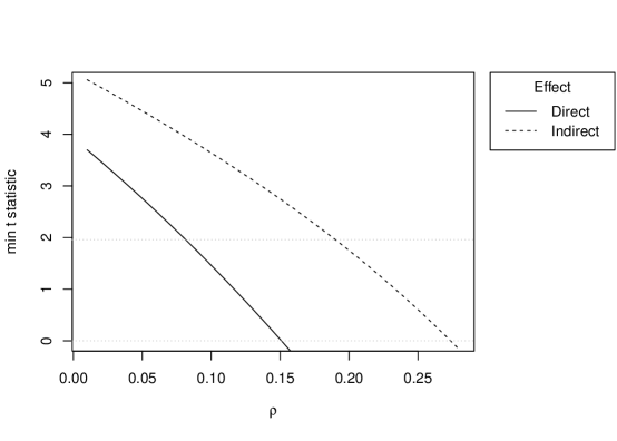
Figure 2: The minimum $t$ statistics of the direct and indirect effects, under the restriction $\max\{R_{y\sim u\mid a,m,c}^{2},R_{m\sim u\mid a,c}^{2},R_{a\sim u\mid c}^{2}\}\leq\rho$. The grey reference lines indicate the $t=1.96$ and $t=0$ thresholds.

Table 1: Sensitivity analysis for Jose (2013)’s mediation analysis. Some reference sample $R^{2}$ values are $\hat{R}_{y\sim a\mid m}^{2}=0.05$, $\hat{R}_{y\sim m\mid a}^{2}=0.25$ and $\hat{R}_{m\sim a}^{2}=0.09$. The R.V. is short for the “robustness value”.

	Est.	Std. Err.	$t$-value	R.V. for Est.	R.V. for $95\%$ C.I.
Direct effect	$0.269$	$0.069$	$3.923$	$0.15$	$0.08$
Indirect effect	$0.215$	$0.041$	$5.205$	$0.27$	$0.19$

7.2 Mediation analysis with multiple mediators

Chong et al. (2016) conduct a randomized study on 219 students of a rural secondary school in the Cajamarca district of Peru during the 2009 school year. They were interested in whether or not the iron deficiency could contribute to the intergenerational persistence of poverty, by affecting the school performance and aspirations for anemic students. They encouraged students to visit the clinic daily to take an iron pill. They randomly assigned students to be exposed multiple times to one of the following three videos: in the first “soccer” group, a popular soccer player was encouraging iron supplements to maximize energy; in the second “physician” group, a doctor was encouraging iron supplements for overall health; in the third “placebo” group, the video did not mention iron at all. They measured various variables of the students after randomization, such as the anemia status at the follow-up survey, the cognitive function measured by the cognitive Wii game, and the school performance measured by average grade in the third and fourth quarters of 2009.

We reanalyze their data. We are interested in the effect of the video assignment $a$ on the school performance $y$, with the anemia status $m_{1}$ and cognitive function $m_{2}$ as mediators. We focus on two levels of the exposure $a$: the “physician” group and the “placebo” group. The covariates $c$ include the gender, class level, anemia status at baseline survey, household monthly income, electricity in home, mother’s years of education. By the Baron–Kenny approach, the estimate for the direct effect is $0.221$, with the $95\%$ confidence interval $[-0.167,0.609]$, and the estimate for the indirect effect is $0.138$, with the $95\%$ confidence interval $[-0.017,0.293]$. Neither is significant.

For illustration purposes, we only assess the sensitivity of the point estimates with respect to unmeasured confounding between the mediator and outcome. By Theorems 3–4, it is not restrictive to assume $u$ is a scalar to compute the robustness values, since $R_{a\sim u\mid c}^{2}=0$ from the design. Figure 2 shows the minimum $t$ statistics under the condition $\max\{R_{y\sim u\mid a,m,c}^{2},R_{u\sim m\mid a,c}^{2}\}\leq\rho$. Table 2 reports some statistics of the direct and indirect effects and their robustness values for the point estimates.

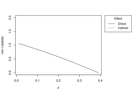
Figure 3: The minimum $t$ statistics of the direct effect and indirect effect, under the restriction $\max\{R_{y\sim u\mid a,m,c}^{2},\|R_{m\sim u\mid a,c}\|_{2}^{2}\}\leq\rho$. The grey reference lines indicate the $t=1.96$ and $t=0$ thresholds.

Table 2: Sensitivity analysis for mediation analysis based on Chong et al. (2016)’s study. Some reference sample $R^{2}$ values are $\max_{j}\hat{R}_{y\sim c_{j}\mid a,c_{-j},m}^{2}=0.113$ and $\max_{j}\hat{R}_{c_{j}\sim m\mid a,c_{-j}}^{2}=0.135$. The R.V. is short for the “robustness value”.

	Est.	Std. Err.	$t$-value	R.V. for Est.	R.V. for $95\%$ C.I.
Direct effect	0.221	0.205	1.079	0.38	0.00
Indirect effect	0.138	0.087	1.586	0.26	0.00

Next, we report some sensitivity bounds with formal benchmarking. We consider the constraint $k_{a}^{(j)}=0$, $k_{m}^{(j)}\leq 1$, and $k_{y}^{(j)}\leq 1$ in (26) for any single covariate $c_{j}$, and we report the worst point estimate for the direct and indirect effects. From Figure 4, if the strength of unmeasured confounder could be as large as any single missing covariate, the worst point estimates would be still away from $0$.

Since the gender variable is the most important covariate in Figure 4, we focus on the specific covariate and report the minimum point estimates under the constraint $k_{a}^{(j)}=0$, $k_{m}^{(j)}\leq\Delta$, and $k_{y}^{(j)}\leq\Delta$ with varying $\Delta$. From Figure 5, only if the strength of unmeasured confounder could be at least $3.9$ times as a missing gender variable, the point estimate for the indirect effect could be reduced to $0$; and only if the strength of unmeasured confounder could be at least $5.5$ times as a missing gender variable, the point estimate for the direct effect could be reduced to $0$.

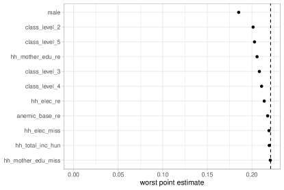
(a) direct effect

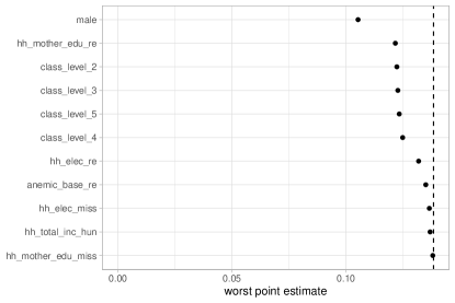
(b) indirect effect

Figure 4: The worst point estimates under the constraint $k_{a}^{(j)}=0$, $k_{m}^{(j)}\leq 1$, $k_{y}^{(j)}\leq 1$ for each covariate $c_{j}$. The reference lines indicate the observed point estimates.

Figure 5: The worst point estimates under the constraint $k_{a}^{(j)}=0$, $k_{m}^{(j)}\leq\Delta$, $k_{y}^{(j)}\leq\Delta$ for the gender variable $c_{j}$.

Discussion

Theorems 1–2 underpin our sensitivity analysis methods. The linear regression formulation is particular useful for the Baron–Kenny approach. Recently, Cinelli et al. (2019) extend it to sensitivity analysis in linear structural causal models, and Cinelli and Hazlett (2022) extend it to sensitivity analysis in the linear instrumental variable model. It is of interest to further explore the applications of Theorems 1–2.

Chernozhukov et al. (2021) provide an extension based on the partially linear model. It is of great interest to extend them to accommodate general nonlinear models based on nonparametric $R^{2}$. VanderWeele (2015) surveys many advanced approaches for mediation analysis based on general definitions of direct and indirect effects. Despite the serious efforts made by VanderWeele (2010), Tchetgen and Shpitser (2012) and Ding and Vanderweele (2016), general sharp and interpretable sensitivity analysis methods are still lacking in the literature. This is an open research direction.

With multiple mediators, we follow the formulation of VanderWeele and Vansteelandt (2013) and view the whole vector $m$ as the mediator. Sometimes, it is of scientific interest to model the causal mechanisms among the mediators and decompose the total effect of the exposure on the outcome into path-specific effects (Avin et al. 2005; Miles et al. 2017). Due to the possible unmeasured confounding, it is important to develop a sensitivity analysis method for path-specific effects. We leave it to future research.

We focus on a single mediator or a low dimensional vector of mediators. Modern genetic studies often have high dimensional mediators (Song et al. 2020; Zhou et al. 2020; Yang et al. 2021). It is important to extend our sensitivity analysis method to handle this more challenging setting. Moreover, Song et al. (2020) and Yang et al. (2021) discuss alternative measures of mediation. It is curious to extend our results to those measures.

Supplementary material

Section A provides a guidance to our R package BaronKennyU.

Section B presents the parallel results based on Cinelli and Hazlett (2020)’s sample least squares under homoskedasticity. We also discuss the difficulties for robust standard errors under this formulation.

Section C presents the sensitivity analysis method for the Baron–Kenny approach based on the difference method.

Section D presents a simulation study on how much we miss if we assume $u$ is a scalar to compute robustness values for mediation.

Section E presents the proofs.

Appendix A R package: BaronKennyU

We provide an R package BaronKennyU to conduct the sensitivity analysis for the Baron–Kenny approach. The package contains R functions to compute the sensitivity bounds with prespecified $R$ parameters, to compute the robustness values, and to report the sensitivity bounds with formal benchmarking. The package can be installed by the R command

devtools::install_github("mingrui229/BaronKennyU")

First, with prespecified $R$ parameters, the R functions bku_direct and bku_indirect compute the point estimate, standard error, and $t$ statistic for the direct and indirect effects, respectively.

Second, the R function bku_rv computes the robustness values for both point estimates and 95% confidence intervals. It returns a summary table like Table 1 or Table 2. The argument randomized indicates if the exposure is randomized. The argument vector_u indicates if the unmeasured confounder $u$ is a vector. For advanced users, we also provide inner R functions bku_rv_direct and bku_rv_indirect to compute the robustness values for direct and indirect effects, respectively. The argument rho_values is the set of candidate $\rho$ to find the robustness values. The default value of argument rho_values is c(1:99)/100. Thus, by default, it computes the robustness values with two decimal digits. Users can change the values of rho_values to compute the robustness values of more accuracy.

Third, the R function bku_fb computes the worst point estimate and $t$ statistic with formal benchmarking for the direct and indirect effects. Besides the data $a$, $m$, $y$, $c_{j}$ and $c_{-j}$, users also need to specify the upper bounds of $k_{a}^{(j)}$, $k_{m}^{(j)}$, $k_{y}^{(j)}$ in (26).

We take the example in Section 7.2 to illustrate the usage of the above R functions. First, with prespecified $R$ parameters $\{R_{y\sim u\mid a,m,c}=0.6,R_{m\sim u\mid a,c}=(0.5,0.5)^{\mathrm{\scriptscriptstyle T}},R_{a\sim u\mid c}=0\}$, we can compute the sensitivity bound for the direct and indirect effects using the R code

bku_direct(y = y, m = m, a = a, c = c, Ry = 0.6, Rm = c(0.5, 0.5), Ra = 0)
bku_indirect(y = y, m = m, a = a, c = c, Ry = 0.6, Rm = c(0.5, 0.5), Ra = 0)

Second, we can compute the robustness values using the R code

bku_rv(y = y, m = m, a = a, c = c, randomized = T)

Third, with prespecified upper bounds $k_{a}^{(j)}=0$, $k_{m}^{(j)}\leq 1$, $k_{y}^{(j)}\leq 1$ in (26) for covariate $c_{1}$, we can compute the sensitivity bounds with formal benchmarking

bku_fb(y = y, m = m, a = a, c = c, j = 1, ky_bound = 1, km_bound = 1, ka_bound = 0)

Appendix B Sensitivity analysis based on Cinelli and Hazlett (2020)’s original strategy of sample least squares

B.1 Sensitivity analysis for the coefficients in sample least squares

Consider the long and short sample least squares regressions with and without $U$:

$$\begin{split}Y&=A\hat{\gamma}_{1}^{\textup{unobs}}+C\hat{\gamma}_{2}^{\textup{unobs}}+U\hat{\gamma}_{3}^{\textup{unobs}}+Y_{\perp A,C,U},\\ Y&=A\hat{\gamma}_{1}^{\textup{obs}}+C\hat{\gamma}_{2}^{\textup{obs}}+Y_{\perp A,C},\end{split}$$ (S1)

where $Y,A,U$ are $n\times 1$ vectors and $C$ is an $n\times p$ matrix including the column of $1$’s. Recall the definition of the sample $R^{2}$.

Definition S1.

For $n\times 1$ vector $Y$, $n\times p$ matrix $X$ and $n\times q$ matrix $Z$, define the sample $R^{2}$ of $Y$ on $X$ as $R_{Y\sim X}^{2}=1-\hat{\mathrm{var}}(Y_{\perp X})/\hat{\mathrm{var}}(Y)$ if $\hat{\mathrm{var}}(Y)\not=0$, and the sample partial $R^{2}$ of $Y$ on $X$ given $Z$ as $R_{Y\sim X\mid Z}^{2}=1-\hat{\mathrm{var}}(Y_{\perp X,Z})/\hat{\mathrm{var}}(Y_{\perp Z})$ if $\hat{\mathrm{var}}(Y_{\perp X})\not=0$.

We remark that the notations $\hat{R}_{y\sim x\mid z}^{2}$ in the main paper and $R_{Y\sim X\mid Z}^{2}$ here are exactly the same in mathematics. In this section, we use the notation $R_{Y\sim X\mid Z}^{2}$ because we want to emphasize that they are sample-level $R^{2}$ parameters, but not estimators of population $R^{2}$ based on the observed data.

Let $\hat{\mathrm{se}}(\cdot)$ denote the classic standard error of the least squares coefficient under the homoskedasticity assumption. The following Theorem S1 is the basis for the sensitivity analysis using Cinelli and Hazlett (2020)’s original strategy.

Theorem S1.

Consider the regressions in (S1) with $n\times 1$ vectors $Y,A,U$ and $n\times p$ matrix $C$. Assume $\hat{\mathrm{cov}}\{(Y,A,U)_{\perp C}\}$ is invertible.

(i) We have

$$\hat{\gamma}_{1}^{\textup{unobs}}=\hat{\gamma}_{1}^{\textup{obs}}+S\left(\frac{R_{Y\sim U\mid A,C}^{2}R_{A\sim U\mid C}^{2}}{1-R_{A\sim U\mid C}^{2}}\right)^{1/2}\left\{\frac{\hat{\mathrm{var}}(Y_{\perp A,C})}{\hat{\mathrm{var}}(A_{\perp C})}\right\}^{1/2},$$ (S2)

and

$$\hat{\mathrm{se}}(\hat{\gamma}_{1}^{\textup{unobs}})=\hat{\mathrm{se}}(\hat{\gamma}_{1}^{\textup{obs}})\left(\frac{1-R_{Y\sim U\mid A,C}^{2}}{1-R_{A\sim U\mid C}^{2}}\frac{\mathrm{df}}{\mathrm{df}-1}\right)^{1/2},$$ (S3)

where

$$S=\mathrm{sgn}(\hat{\gamma}_{1}^{\textup{unobs}}-\hat{\gamma}_{1}^{\textup{obs}}),\quad\mathrm{df}=n-p-1.$$

(ii) Assume $n\geq p+3$. Given the observed data $\{Y,A,C\}$, the parameters $\{R_{Y\sim U\mid A,C}^{2},R_{A\sim U\mid C}^{2}\}$ can take arbitrary values in $[0,1)^{2}$, and $\{R_{Y\sim U\mid A,C}^{2},R_{A\sim U\mid C}^{2},S\}$ can take arbitrary value in $(0,1)^{2}\times\{-1,1\}$.

Theorem S1(i) is from Cinelli and Hazlett (2020), whereas Theorem S1(ii) on the sharpness is new. Based on Theorem S1, we summarize the sensitivity analysis procedure of Cinelli and Hazlett (2020) in Algorithm S1 below.

Algorithm S1.

A sensitivity analysis procedure for the coefficient $\hat{\gamma}_{1}^{\textup{unobs}}$ based on the regressions in (S1), with prespecified sensitivity parameters $\{R_{Y\sim U\mid A,C}^{2},R_{A\sim U\mid C}^{2},S\}$, where $S=\mathrm{sgn}(\hat{\gamma}_{1}^{\textup{unobs}}-\hat{\gamma}_{1}^{\textup{obs}})$:

1. compute $\hat{\gamma}_{1}^{\textup{unobs}}$ and $\hat{\mathrm{se}}(\hat{\gamma}_{1}^{\textup{unobs}})$ by (S2) and (S3);

2. return the point estimate $\hat{\gamma}_{1}^{\textup{unobs}}$, standard error $\hat{\mathrm{se}}(\hat{\gamma}_{1}^{\textup{unobs}})$, and $t$ statistic $\hat{\gamma}_{1}^{\textup{unobs}}/\hat{\mathrm{se}}(\hat{\gamma}_{1}^{\textup{unobs}})$.

If we specify $\{R_{Y\sim U\mid A,C}^{2},R_{A\sim U\mid C}^{2},S\}$, then we apply Theorem S1 directly; if we only specify $\{R_{Y\sim U\mid A,C}^{2},R_{A\sim U\mid C}^{2}\}$ without $S$, then we report the point estimate, standard error, and $t$ statistic with the worst case of the sign.

B.2 Sensitivity analysis for the direct effect

Consider the long and short sample least squares regressions with $U$

$$\begin{split}M&=A\hat{\beta}_{1}^{\textup{unobs}}+C\hat{\beta}_{2}^{\textup{unobs}}+U\hat{\beta}_{3}^{\textup{unobs}}+M_{\perp A,C,U},\\ Y&=A\hat{\theta}_{1}^{\textup{unobs}}+C\hat{\theta}_{2}^{\textup{unobs}}+M\hat{\theta}_{3}^{\textup{unobs}}+U\hat{\theta}_{4}^{\textup{unobs}}+Y_{\perp A,C,M,U},\\ \end{split}$$ (S4)

and without $U$

$$\begin{split}M&=A\hat{\beta}_{1}^{\textup{obs}}+C\hat{\beta}_{2}^{\textup{obs}}+M_{\perp A,C},\\ Y&=A\hat{\theta}_{1}^{\textup{obs}}+C\hat{\theta}_{2}^{\textup{obs}}+M\hat{\theta}_{3}^{\textup{obs}}+Y_{\perp A,C,M},\end{split}$$ (S5)

respectively, where $Y,M,A,U$ are $n\times 1$ vectors and $C$ is an $n\times p$ matrix. For the direct effect, the observed estimator is $\hat{\theta}_{1}^{\textup{obs}}$ with classical standard error $\hat{\mathrm{se}}(\hat{\theta}_{1}^{\textup{obs}})$, and the unobserved estimator is $\hat{\theta}_{1}^{\textup{unobs}}$ with classical standard error $\hat{\mathrm{se}}(\hat{\theta}_{1}^{\textup{unobs}})$. Apply Theorem S1 to obtain

$$\hat{\theta}_{1}^{\textup{unobs}}=\hat{\theta}_{1}^{\textup{obs}}+S_{1}\left(\frac{R_{Y\sim U\mid A,M,C}^{2}R_{A\sim U\mid M,C}^{2}}{1-R_{A\sim U\mid M,C}^{2}}\right)^{1/2}\left\{\frac{\hat{\mathrm{var}}(Y_{\perp A,M,C})}{\hat{\mathrm{var}}(A_{\perp C,M})}\right\}^{1/2},$$ (S6)

and

$$\hat{\mathrm{se}}(\hat{\theta}_{1}^{\textup{unobs}})=\hat{\mathrm{se}}(\hat{\theta}_{1}^{\textup{obs}})\left(\frac{n-p-2}{n-p-3}\cdot\frac{1-R_{Y\sim U\mid A,M,C}^{2}}{1-R_{A\sim U\mid M,C}^{2}}\right)^{1/2}.$$ (S7)

where $S_{1}=\mathrm{sgn}(\hat{\theta}_{1}^{\textup{unobs}}-\hat{\theta}_{1}^{\textup{obs}})$. Unfortunately, $R_{A\sim U\mid C,M}^{2}$ is not a parameter corresponding to the factorization of the joint distribution based on Figure 1(b). Similar to Proposition 1, we can express $R_{A\sim U\mid C,M}^{2}$ using natural parameters in Proposition S1 below.

Proposition S1.

Assume $\hat{\mathrm{cov}}\{(Y,M,A,U)_{\perp C}\}$ is invertible for $n\times 1$ vectors $Y,M,A,U$ and $n\times p$ matrix $C$. We have

$$R_{A\sim U\mid C,M}^{2}=\begin{cases}1-\frac{(1-R_{A\sim U\mid C}^{2})(1-R_{M\sim U\mid A,C}^{2})}{1-(S_{2}v_{1}+v_{2})^{2}}&\text{if }R_{M\sim U\mid A,C}^{2}\not=0,\\ 1-\frac{1-R_{A\sim U\mid C}^{2}}{1-v_{1}^{2}}&\text{if }R_{M\sim U\mid A,C}^{2}=0,\\ \end{cases}$$

where

$$v_{1} = (R_{A\sim U\mid C}^{2}R_{M\sim A\mid C}^{2})^{1/2},$$

$$v_{2} = \left\{R_{M\sim U\mid A,C}^{2}(1-R_{A\sim U\mid C}^{2})(1-R_{M\sim A\mid C}^{2})\right\}^{1/2},$$

$$S_{2} = \mathrm{sgn}(\hat{\beta}_{1}^{\textup{obs}})\cdot\mathrm{sgn}(\hat{\beta}_{1}^{\textup{obs}}-\hat{\beta}_{1}^{\textup{unobs}}).$$

Define

$$R_{U}^{2}=\{R_{Y\sim U\mid A,M,C}^{2},R_{M\sim U\mid A,C}^{2},R_{A\sim U\mid C}^{2}\}$$

as the set of $R^{2}$ parameters, which correspond to the natural factorization of the likelihood based on Figure 1(b). With fixed $R_{U}^{2}$ and the signs of the bias terms, we can first compute $R_{A\sim U\mid M,C}^{2}$ and then obtain the point estimate $\hat{\theta}_{1}^{\textup{unobs}}$ and standard error $\hat{\mathrm{se}}(\hat{\theta}_{1}^{\textup{unobs}})$. We summarize the sensitivity analysis procedure in Algorithm S2 below.

Algorithm S2.

A sensitivity analysis procedure for the direct effect $\hat{\theta}_{1}^{\textup{unobs}}$ based on the regressions in (S4) and (S5), with prespecified sensitivity parameters $\{R_{U}^{2},S_{1},S_{2}\}$, where $S_{1}=\mathrm{sgn}(\hat{\theta}_{1}^{\textup{unobs}}-\hat{\theta}_{1}^{\textup{obs}})$ and $S_{2}=\mathrm{sgn}(\hat{\beta}_{1}^{\textup{obs}})\cdot\mathrm{sgn}(\hat{\beta}_{1}^{\textup{obs}}-\hat{\beta}_{1}^{\textup{unobs}})$:

1. compute $R_{M\sim A\mid C}^{2}$ from the sample least squares fit of the observed data $M$ on $(A,C)$;

2. compute $R_{A\sim U\mid M,C}^{2}$ by Proposition S1;

3. compute $\hat{\theta}_{1}^{\textup{unobs}}$ and $\hat{\mathrm{se}}(\hat{\theta}_{1}^{\textup{unobs}})$ by (S6) and (S7);

4. return the point estimate $\hat{\theta}_{1}^{\textup{unobs}}$, standard error $\hat{\mathrm{se}}(\hat{\theta}_{1}^{\textup{unobs}})$, and $t$ statistic $\hat{\theta}_{1}^{\textup{unobs}}/\hat{\mathrm{se}}(\hat{\theta}_{1}^{\textup{unobs}})$.

Without specifying $S_{1}$ and $S_{2}$, we report the results based on $R_{U}^{2}$ with the worst case of the signs. The sensitivity bound obtained by Algorithm S2 is sharp by Corollary 1 below.

Corollary S1.

Assume $\hat{\mathrm{cov}}\{(Y,M,A,U)_{\perp C}\}$ is invertible for $n\times 1$ vectors $Y,M,A,U$ and $n\times p$ matrix $C$, and $n\geq p+4$. Given the observed data $\{Y,M,A,C\}$, the parameters $R_{U}^{2}$ can take arbitrary values in $[0,1)^{3}$, and if $\hat{\beta}_{1}^{\textup{obs}}\not=0$, then $\{R_{U}^{2},S_{1},S_{2}\}$ can take arbitrary values in $(0,1)^{3}\times\{-1,1\}^{2}\setminus E_{0}$, where $E_{0}$ is the set of all possible parameters such that $R_{A\sim U\mid M,C}^{2}=0$.

If $\hat{\beta}_{1}^{\textup{obs}}=0$, then $S_{2}$ must be $0$; and if $R_{A\sim U\mid M,C}^{2}=0$, then $S_{1}$ must be $0$. The exceptional set $E_{0}$ in Corollary S1 refers to an edge case in which the bias of the direct effect is $0$. Given the observed data $\{Y,M,A,C\}$, the $R_{M\sim A\mid C}^{2}$ is fixed and observable, and therefore, $E_{0}$ can be determined by Proposition S1.

B.3 Sensitivity analysis for the indirect effect

We only consider the product method for the indirect effect because the difference method is more difficult: besides the effort to represent the unnatural $R^{2}$ parameters by natural ones, the inference of the difference method estimator depends on the robust standard error, which is not permitted by Cinelli and Hazlett (2020)’s original result. See Section B.4 below for more details.

For the indirect effect, the observed estimator is $\hat{\beta}_{1}^{\textup{obs}}\hat{\theta}_{3}^{\textup{obs}}$ and the unobserved estimator is $\hat{\beta}_{1}^{\textup{unobs}}\hat{\theta}_{3}^{\textup{unobs}}$. By the delta method, the observed classical standard error is $\{(\hat{\beta}_{1}^{\textup{obs}})^{2}\hat{\mathrm{se}}^{2}(\hat{\theta}_{3}^{\textup{obs}})+(\hat{\theta}_{3}^{\textup{obs}})^{2}\hat{\mathrm{se}}^{2}(\hat{\beta}_{1}^{\textup{obs}})\}^{1/2}$, and the unobserved classical standard error is

$$\{(\hat{\beta}_{1}^{\textup{unobs}})^{2}\hat{\mathrm{se}}^{2}(\hat{\theta}_{3}^{\textup{unobs}})+(\hat{\theta}_{3}^{\textup{unobs}})^{2}\hat{\mathrm{se}}^{2}(\hat{\beta}_{1}^{\textup{unobs}})\}^{1/2}.$$ (S8)

Apply Theorem S1 to obtain

$$\begin{split}\hat{\beta}_{1}^{\textup{unobs}}&=\hat{\beta}_{1}^{\textup{obs}}+S_{3}\left(\frac{R_{M\sim U\mid A,C}^{2}R_{A\sim U\mid C}^{2}}{1-R_{A\sim U\mid C}^{2}}\right)^{1/2}\left\{\frac{\hat{\mathrm{var}}(M_{\perp A,C})}{\hat{\mathrm{var}}(A_{\perp C})}\right\}^{1/2},\\ \hat{\theta}_{3}^{\textup{unobs}}&=\hat{\theta}_{3}^{\textup{obs}}+S_{4}\left(\frac{R_{Y\sim U\mid A,C,M}^{2}R_{M\sim U\mid A,C}^{2}}{1-R_{M\sim U\mid A,C}^{2}}\right)^{1/2}\left\{\frac{\hat{\mathrm{var}}(Y_{\perp A,C,M})}{\hat{\mathrm{var}}(M_{\perp A,C})}\right\}^{1/2},\end{split}$$ (S9)

and

$$\begin{split}\hat{\mathrm{se}}(\hat{\beta}_{1}^{\textup{unobs}})&=\hat{\mathrm{se}}(\hat{\beta}_{1}^{\textup{obs}})\left(\frac{n-p-1}{n-p-2}\cdot\frac{1-R_{M\sim U\mid A,C}^{2}}{1-R_{A\sim U\mid C}^{2}}\right)^{1/2},\\ \hat{\mathrm{se}}(\hat{\theta}_{3}^{\textup{unobs}})&=\hat{\mathrm{se}}(\hat{\theta}_{3}^{\textup{obs}})\left(\frac{n-p-2}{n-p-3}\cdot\frac{1-R_{Y\sim U\mid A,M,C}^{2}}{1-R_{M\sim U\mid A,C}^{2}}\right)^{1/2},\end{split}$$ (S10)

where $S_{3}=\mathrm{sgn}(\hat{\beta}_{1}^{\textup{unobs}}-\hat{\beta}_{1}^{\textup{obs}})$ and $S_{4}=\mathrm{sgn}(\hat{\theta}_{3}^{\textup{unobs}}-\hat{\theta}_{3}^{\textup{obs}})$. The above formulas (S9)–(S10) are parameterized by natural parameters in $R_{U}^{2}$. For fixed $R_{U}^{2}$ and the signs of some bias terms, we can directly obtain the point estimate $\hat{\beta}_{1}^{\textup{unobs}}\hat{\theta}_{3}^{\textup{unobs}}$ and standard error $\hat{\mathrm{se}}(\hat{\beta}_{1}^{\textup{unobs}}\hat{\theta}_{3}^{\textup{unobs}})$. We summarize the sensitivity analysis procedure in Algorithm S3 below.

Algorithm S3.

A sensitivity analysis procedure for the indirect effect $\hat{\beta}_{1}^{\textup{unobs}}\hat{\theta}_{3}^{\textup{unobs}}$ based on the regressions in (S4) and (S5), with prespecified sensitivity parameters $\{R_{U}^{2},S_{3},S_{4}\}$, where $S_{3}=\mathrm{sgn}(\hat{\beta}_{1}^{\textup{unobs}}-\hat{\beta}_{1}^{\textup{obs}})$ and $S_{4}=\mathrm{sgn}(\hat{\theta}_{3}^{\textup{unobs}}-\hat{\theta}_{3}^{\textup{obs}})$:

1. compute $\hat{\beta}_{1}^{\textup{unobs}}$, $\hat{\theta}_{3}^{\textup{unobs}}$, $\hat{\mathrm{se}}(\hat{\beta}_{1}^{\textup{unobs}})$ and $\hat{\mathrm{se}}(\hat{\theta}_{3}^{\textup{unobs}})$ by (S9) and (S10);

2. compute the standard error $\hat{\mathrm{se}}(\hat{\beta}_{1}^{\textup{unobs}}\hat{\theta}_{3}^{\textup{unobs}})$ by (S8);

3. return the point estimate $\hat{\beta}_{1}^{\textup{unobs}}\hat{\theta}_{3}^{\textup{unobs}}$, standard error $\hat{\mathrm{se}}(\hat{\beta}_{1}^{\textup{unobs}}\hat{\theta}_{3}^{\textup{unobs}})$, and $t$ statistic
   $\hat{\beta}_{1}^{\textup{unobs}}\hat{\theta}_{3}^{\textup{unobs}}/\hat{\mathrm{se}}(\hat{\beta}_{1}^{\textup{unobs}}\hat{\theta}_{3}^{\textup{unobs}})$.

Again, without specifying $S_{3}$ and $S_{4}$, we report the results based on $R_{U}^{2}$ with the worst case of the signs. The sensitivity bound obtained by Algorithm S3 is sharp by Corollary S2 below.

Corollary S2.

Assume $\hat{\mathrm{cov}}\{(Y,M,A,U)_{\perp C}\}$ is invertible for $n\times 1$ vectors $Y,M,A,U$ and $n\times p$ matrix $C$, and $n\geq p+4$. Given the observed data $\{Y,M,A,C\}$, the parameters $\{R_{U}^{2},S_{3},S_{4}\}$ can take arbitrary values in $(0,1)^{3}\times\{-1,1\}^{2}$.

B.4 Difficulty of Cinelli and Hazlett (2020)’s strategy for robust standard errors

Theorem S1 provides a useful tool for sensitivity analysis of coefficients from sample least squares regression. As an important limitation, Cinelli and Hazlett (2020) only consider the ratio of classical standard errors. Unfortunately, it is nontrivial to extend their result to the ratio of robust standard errors. Let $\tilde{\mathrm{se}}$ denote the robust standard error. We can rewrite the ratio of the robust standard errors as

$$\frac{\tilde{\mathrm{se}}(\hat{\gamma}_{1}^{\textup{unobs}})}{\tilde{\mathrm{se}}(\hat{\gamma}_{1}^{\textup{obs}})}=\frac{\hat{\mathrm{se}}(\hat{\gamma}_{1}^{\text{obs}})}{\tilde{\mathrm{se}}(\hat{\gamma}_{1}^{\text{obs}})}\cdot\frac{\hat{\mathrm{se}}(\hat{\gamma}_{1}^{\text{unobs}})}{\hat{\mathrm{se}}(\hat{\gamma}_{1}^{\text{obs}})}\cdot\frac{\tilde{\mathrm{se}}(\hat{\gamma}_{1}^{\text{unobs}})}{\hat{\mathrm{se}}(\hat{\gamma}_{1}^{\text{unobs}})},$$ (S11)

where the first term in (S11) is observable, the second term in (S11) is the ratio of classic standard error, and the third term in (S11) is unobservable and difficult to deal with because its finite-sample variance depends on higher moments of the unobserved confounder. In particular, we can prove that the third term in (S11) converges in probability to

$$\frac{E(y_{\perp a,c,u}^{2}a_{\perp c,u}^{2})}{E(y_{\perp a,c,u}^{2})E(a_{\perp c,u}^{2})}$$

under finite fourth moment assumptions. It is unbounded without further constraints on $u$, which implies that the precise value of the robust standard error depends on some higher order moments that cannot be bounded by the $R^{2}$ parameters. Thus Cinelli and Hazlett (2020)’s original strategy does not easily generalize to deal with heteroskedasticity and model misspecification.

Appendix C Sensitivity analysis for the indirect effect based on the difference method

We assume the mediator $m$ can be a vector. Based on (1), (18) and (19), the true indirect effect by the difference method is $\gamma_{1}-\theta_{1}$. By Theorem 1, for fixed parameters $\{R_{y\sim u\mid a,c}$, $R_{a\sim u\mid c}$, $R_{y\sim u\mid a,m,c}$, $R_{a\sim u\mid m,c}\}$, we can use

$$\hat{\gamma}_{1}=\hat{\gamma}_{1}^{\text{obs}}-\frac{R_{y\sim u\mid a,c}R_{a\sim u\mid c}}{(1-R_{a\sim u\mid c}^{2})^{1/2}}\cdot\left\{\frac{\hat{\mathrm{var}}(Y_{\perp A,C})}{\hat{\mathrm{var}}(A_{\perp C})}\right\}^{1/2}$$ (S12)

to estimate $\gamma_{1}$ and (12) to estimate $\theta_{1}$. Unfortunately, $R_{a\sim u\mid m,c}$ in (12) and $R_{y\sim u\mid a,c}$ in (S12) are not natural parameters. Nevertheless, Proposition 2 already shows that $R_{a\sim u\mid m,c}$ can be represented by the natural sensitivity parameters $R_{m\sim u\mid a,c}$ and $R_{a\sim u\mid c}$. Proposition S2 below further shows that $R_{y\sim u\mid a,c}$ can be represented by the natural sensitivity parameters $R_{y\sim u\mid a,m,c}$ and $R_{m\sim u\mid a,c}$.

Proposition S2.

Assume $\mathrm{cov}\{(y,m,a,u)_{\perp c}\}$ is invertible for possibly vector $m,c$ but scalar $y,a,u$. We have

$$R_{y\sim u\mid a,c}=(1-\|R_{m\sim u\mid a,c}\|_{2}^{2})^{1/2}(1-\|R_{y\sim m\mid a,c}\|_{2}^{2})^{1/2}R_{y\sim u\mid a,m,c}+R_{y\sim m\mid a,c}R_{m\sim u\mid a,c}.$$

Therefore, with prespecified $R_{u}$, we can first estimate $R_{a\sim u\mid m,c}$ by Proposition 2 and $R_{y\sim u\mid a,c}$ by Proposition S2, and then obtain the point estimate $\hat{\theta}_{1}-\hat{\gamma}_{1}$. We summarize the sensitivity analysis procedure in Algorithm S4 below.

Algorithm S4.

A sensitivity analysis procedure for the indirect effect $\tilde{\theta}_{1}-\tilde{\gamma}_{1}$ based on the regressions in (1) and (18)–(19), with prespecified sensitivity parameters $R_{u}$:

1. estimate $R_{m\sim a\mid c}$, $\mathrm{cov}(m_{\perp c})$, $\mathrm{cov}(m_{\perp a,c})$ using the observed data $(M,A,C)$;

2. estimate $R_{a\sim u\mid m,c}$ by Proposition 2 with the estimated $R_{m\sim a\mid c}$, $\mathrm{cov}(m_{\perp c})$, $\mathrm{cov}(m_{\perp a,c})$ from (a);

3. estimate $R_{y\sim m\mid a,c}$ using the observed data $(Y,M,A,C)$;

4. estimate $R_{y\sim u\mid a,c}$ by Proposition S2 with the estimated $R_{m\sim y\mid a,c}$ from (c);

5. compute $\hat{\theta}_{1}$ by (12) and $\hat{\gamma}_{1}$ by (S12) with the estimated $R_{a\sim u\mid m,c}$ and $R_{y\sim u\mid a,c}$ from (b) and (d);

6. obtain the standard error $\hat{\mathrm{se}}(\hat{\theta}_{1}-\hat{\gamma}_{1})$ by the nonparametric bootstrap;

7. return the point estimate $\hat{\theta}_{1}-\hat{\gamma}_{1}$, standard error $\hat{\mathrm{se}}(\hat{\theta}_{1}-\hat{\gamma}_{1})$, and $t$ statistic $(\hat{\theta}_{1}-\hat{\gamma}_{1})/\hat{\mathrm{se}}(\hat{\theta}_{1}-\hat{\gamma}_{1})$.

The sensitivity bound using the product method is exactly the same as the sensitivity bound using the difference method. This is because the product method is equivalent to the difference method, and the two algorithms have exactly the same sensitivity parameters $R_{u}$. However, we do not recommend the difference method due to its complexity in representing unnatural $R$ parameters $R_{a\sim u\mid m,c}$ and $R_{y\sim u\mid a,c}$.

Appendix D A simulation study of robustness values for mediation

By Theorem 4, it could be restrictive to assume $u$ is a scalar to compute the robustness values for the indirect effect in general. Next, we study how much we miss if we assume $u$ is a scalar by simulations. We consider the following simulation setting. The exposure $a$ follows a standard normal distribution $N(0,1)$. Given $a$, the mediator $m$ follows a multivariate normal distribution with mean $\alpha_{1}a$ and variance $\Sigma$, where

$$\alpha_{1}=\lambda_{1}\left(0,\frac{1}{\mathrm{dim}(m)-1},\frac{2}{\mathrm{dim}(m)-1},...,\frac{\mathrm{dim}(m)-2}{\mathrm{dim}(m)-1},1\right)$$

with $\lambda_{1}$ selected later, and $\Sigma_{ij}=0.5^{|i-j|}$, for all $1\leq i,j\leq\mathrm{dim}(m)$. Given $a$ and $m$, the outcome $y$ follows a normal distribution with mean $a+\alpha_{2}^{\mathrm{\scriptscriptstyle T}}m$ and variance $1$, where

$$\alpha_{2}=\lambda_{2}\left(1,1-\frac{1.5}{\mathrm{dim}(m)-1},1-\frac{3}{\mathrm{dim}(m)-1},...,1-\frac{1.5\{\mathrm{dim}(m)-2\}}{\mathrm{dim}(m)-1},-0.5\right)$$

with $\lambda_{2}$ selected later.

We vary the three factors $\mathrm{dim}(m)\in\{2,4,6\}$, $R_{a\sim m\mid c}^{2}\in\{0.1,0.3,0.5,0.7\}$, $R_{y\sim m\mid a,c}^{2}\in\{0.1,0.3,0.5,0.7\}$ in our simulation design. For the $R^{2}$ parameters, we select $\lambda_{1}>0$ to achieve a specific level of $R_{a\sim m\mid c}^{2}$ and we select $\lambda_{2}>0$ to achieve a specific level of $R_{y\sim a\mid m,c}^{2}$. Tables S1–S2 compare the robustness values with scalar $u$ and vector $u$, for the point estimates and $95\%$ confidence intervals, respectively. Numerically, we can observe that the robustness values with vector $u$ are about $3/4$ times the robustness values with scalar $u$.

We also conduct an ANOVA test to analyze the effect of the three factors on the ratio of robustness values with vector $u$ and with scalar $u$. From Table S3, we can find that the dimension of $m$ is the most important factor. However, we observe that when the dimension of $m$ increases, the average ratio of robustness values increases. Therefore, the higher dimension of $m$ would not lead to a smaller ratio of the robustness values, based on the current simulation results.

Table S1: Simulation results of the average robustness values for point estimates with scalar $u$, over $20$ data replications. The values in the parentheses are the average robustness values for point estimates with vector $u$.

$\mathrm{dim}(m)$	$R_{a\sim m\mid c}^{2}$	$R_{y\sim m\mid a,c}^{2}$
		$0.1$	$0.3$	$0.5$	$0.7$
$2$	$0.1$	0.090 (0.064)	0.126 (0.096)	0.171 (0.136)	0.173 (0.150)
	$0.3$	0.138 (0.104)	0.236 (0.171)	0.236 (0.176)	0.280 (0.220)
	$0.5$	0.125 (0.102)	0.245 (0.185)	0.312 (0.232)	0.364 (0.280)
	$0.7$	0.134 (0.115)	0.264 (0.214)	0.359 (0.279)	0.429 (0.329)
$4$	$0.1$	0.054 (0.036)	0.082 (0.062)	0.078 (0.062)	0.079 (0.064)
	$0.3$	0.071 (0.052)	0.102 (0.072)	0.126 (0.092)	0.118 (0.090)
	$0.5$	0.086 (0.068)	0.116 (0.084)	0.165 (0.119)	0.180 (0.132)
	$0.7$	0.080 (0.067)	0.130 (0.100)	0.162 (0.121)	0.238 (0.172)
$6$	$0.1$	0.036 (0.024)	0.056 (0.040)	0.072 (0.054)	0.061 (0.050)
	$0.3$	0.058 (0.043)	0.089 (0.060)	0.097 (0.069)	0.093 (0.067)
	$0.5$	0.080 (0.061)	0.095 (0.064)	0.119 (0.078)	0.118 (0.082)
	$0.7$	0.076 (0.061)	0.118 (0.085)	0.103 (0.069)	0.179 (0.126)

Table S2: Simulation results of the average robustness values for $95\%$ confidence intervals with scalar $u$, over $20$ data replications. The values in the parentheses are the average robustness values for $95\%$ confidence intervals with vector $u$.

$\mathrm{dim}(m)$	$R_{a\sim m\mid c}^{2}$	$R_{y\sim m\mid a,c}^{2}$
		$0.1$	$0.3$	$0.5$	$0.7$
$2$	$0.1$	0.002 (0.001)	0.018 (0.013)	0.062 (0.049)	0.060 (0.052)
	$0.3$	0.024 (0.020)	0.121 (0.086)	0.124 (0.092)	0.172 (0.134)
	$0.5$	0.022 (0.015)	0.128 (0.094)	0.207 (0.152)	0.265 (0.199)
	$0.7$	0.035 (0.031)	0.148 (0.118)	0.259 (0.199)	0.342 (0.258)
$4$	$0.1$	0.000 (0.000)	0.006 (0.004)	0.004 (0.002)	0.010 (0.008)
	$0.3$	0.005 (0.003)	0.016 (0.011)	0.024 (0.017)	0.020 (0.014)
	$0.5$	0.005 (0.004)	0.018 (0.012)	0.048 (0.034)	0.062 (0.045)
	$0.7$	0.006 (0.006)	0.026 (0.020)	0.057 (0.042)	0.121 (0.087)
$6$	$0.1$	0.000 (0.000)	0.000 (0.000)	0.006 (0.004)	0.000 (0.000)
	$0.3$	0.002 (0.002)	0.008 (0.005)	0.014 (0.009)	0.012 (0.010)
	$0.5$	0.002 (0.002)	0.014 (0.010)	0.018 (0.010)	0.020 (0.013)
	$0.7$	0.005 (0.004)	0.013 (0.010)	0.015 (0.009)	0.065 (0.042)

Table S3: ANOVA analysis for the ratio of robustness values with vector $u$ and with scalar $u$.

Ratio of robustness values	Factor	df	MSE	$F$-value	$p$-value
point estimate	$\mathrm{dim}(m)$	2	0.387	26.075	$9.63\times 10^{-12}$
	$R_{a\sim m\mid c}^{2}$	3	0.076	5.086	0.0017
	$R_{y\sim m\mid a,c}^{2}$	3	0.044	2.992	0.0301
95% confidence interval	$\mathrm{dim}(m)$	2	0.215	9.250	$1.17\times 10^{-4}$
	$R_{a\sim m\mid c}^{2}$	3	0.119	5.125	0.0017
	$R_{y\sim m\mid a,c}^{2}$	3	0.057	2.465	0.0618

Appendix E Proofs

E.1 Some useful Lemmas

Lemma S1.

For scalar $y$ and vectors $x$ and $z$, we have

$$R_{y\sim z\mid x}^{2}=\frac{R_{y\sim(z,x)}^{2}-R_{y\sim x}^{2}}{1-R_{y\sim x}^{2}}=1-\frac{(1-R_{y\sim x\mid z}^{2})(1-R_{y\sim z}^{2})}{1-R_{y\sim x}^{2}}$$

if $\mathrm{cov}\{(x,y,z)\}$ is invertible.

Proof of Lemma S1.

By Definition 2,

$$R_{y\sim z\mid x}^{2}=\frac{\mathrm{var}(y_{\perp x})-\mathrm{var}(y_{\perp x,z})}{\mathrm{var}(y_{\perp x})}=\frac{R_{y\sim(z,x)}^{2}-R_{y\sim x}^{2}}{1-R_{y\sim x}^{2}}.$$ (S13)

Swapping $x$ and $z$, we also have

$$R_{y\sim x\mid z}^{2}=\frac{R_{y\sim(x,z)}^{2}-R_{y\sim z}^{2}}{1-R_{y\sim z}^{2}}.$$ (S14)

Combining (S13)–(S14), we obtain the desired result. ∎

Lemma S2.

For vectors $x,y,z$,

$$\begin{split}\mathrm{cov}(y_{\perp x})&=\mathrm{cov}(y)-\mathrm{cov}(y,x)\mathrm{cov}(x)^{-1}\mathrm{cov}(x,y),\\ \mathrm{cov}(y_{\perp x},z_{\perp x})&=\mathrm{cov}(y,z)-\mathrm{cov}(y,x)\mathrm{cov}(x)^{-1}\mathrm{cov}(x,z),\\ \end{split}$$

if $\mathrm{cov}(x)$ is invertible.

Proof of Lemma S2.

Consider the population least squares $y=\beta x+y_{\perp x}$ with $\beta=\mathrm{cov}(y,x)\mathrm{cov}(x)^{-1}$ and $y_{\perp x}=y-\mathrm{cov}(y,x)\mathrm{cov}(x)^{-1}x$. Similarly, $z_{\perp x}=z-\mathrm{cov}(z,x)\mathrm{cov}(x)^{-1}x$. We can obtain the desired results by direct calculation. ∎

Lemma S3.

For centered vectors $x,y,z$,

$$R_{y\sim z\mid x}=\mathrm{cov}(y_{\perp x})^{-1/2}\mathrm{cov}(y)^{1/2}(R_{y\sim z}-R_{y\sim x}R_{x\sim z})\mathrm{cov}(z)^{1/2}\mathrm{cov}(z_{\perp x})^{-1/2},$$

if $\mathrm{cov}\{(x,y,z)\}$ is invertible. Further assume $y$ and $z$ are centered scalars,

$$R_{y\sim z\mid x}=\frac{R_{y\sim z}-R_{y\sim x}R_{x\sim z}}{(1-\|R_{y\sim x}\|_{2}^{2})^{1/2}(1-\|R_{z\sim x}\|_{2}^{2})^{1/2}}.$$

Proof of Lemma S3.

By Lemma S2,

$$\begin{split}&\mathrm{cov}(y_{\perp x})^{-1/2}\mathrm{cov}(y)^{1/2}(R_{y\sim z}-R_{y\sim x}R_{x\sim z})\mathrm{cov}(z)^{1/2}\mathrm{cov}(z_{\perp x})^{-1/2}\\ =&\mathrm{cov}(y_{\perp x})^{-1/2}\left\{\mathrm{cov}(y,z)-\mathrm{cov}(y,x)\mathrm{cov}(x)^{-1}\mathrm{cov}(x,z)\right\}\mathrm{cov}(z_{\perp x})^{-1/2}\\ =&\mathrm{cov}(y_{\perp x})^{-1/2}\mathrm{cov}(y_{\perp x},z_{\perp x})^{-1/2}\mathrm{cov}(z_{\perp x})^{-1/2}\\ =&R_{y\sim z\mid x}.\end{split}$$

If $y$ and $z$ are centered scalars, we have

$$\frac{\mathrm{var}(y_{\perp x})}{\mathrm{var}(y)}=1-R_{y\sim x}^{2}=1-\|R_{y\sim x}\|_{2}^{2}$$

and

$$\frac{\mathrm{var}(z_{\perp x})}{\mathrm{var}(z)}=1-R_{z\sim x}^{2}=1-\|R_{z\sim x}\|_{2}^{2}$$

which imply the desired result. ∎

Lemma S4.

For centered nonzero scalars $y,x,z$, we have

$$R_{y\sim z}^{2}=\left[S(R_{y\sim x}^{2}R_{z\sim x}^{2})^{1/2}+S^{\prime}\{R_{y\sim z\mid x}^{2}(1-R_{y\sim x}^{2})(1-R_{z\sim x}^{2})\}^{1/2}\right]^{2}$$

if $\mathrm{cov}\{(x,y,z)\}$ is invertible, where

$$S=\mathrm{sgn}\{\mathrm{corr}(y,x)\cdot\mathrm{corr}(z,x)\},\quad S^{\prime}=\mathrm{sgn}\{\mathrm{corr}(y_{\perp x},z_{\perp x})\}.$$

Lemma S4 is a direct corollary of Lemma S3.

Lemma S5.

Assume $A$ is symmetric and $C$ is positive definite. Then

$$M=\begin{pmatrix}A&B\\ B^{\mathrm{\scriptscriptstyle T}}&C\end{pmatrix}$$

is positive definite if and only if $A-BC^{-1}B^{\mathrm{\scriptscriptstyle T}}$ is positive definite.

Lemma S5 is a standard property of the Schur complement. We omit its proof.

Lemma S6.

(i) Assume any given random vectors $a,b$ such that the covariance matrix $\mathrm{cov}\{(a,b)\}$ is invertible. For any positive definite matrices

$$\Sigma_{1}=\begin{pmatrix}\Sigma_{aa}&\Sigma_{au}\\ \Sigma_{ua}&\Sigma_{uu}\end{pmatrix},\quad\Sigma_{2}=\begin{pmatrix}\Sigma_{bb\mid a}&\Sigma_{bu\mid a}\\ \Sigma_{ub\mid a}&\Sigma_{uu\mid a}\end{pmatrix},$$

satisfying $\Sigma_{uu\mid a}=\Sigma_{uu}-\Sigma_{ua}\Sigma_{aa}^{-1}\Sigma_{au}$, $\mathrm{cov}(a)=\Sigma_{aa}$, and $\mathrm{cov}(b_{\perp a})=\Sigma_{bb\mid a}$, there exists a vector $u$ such that $\mathrm{cov}\{(a,u)\}=\Sigma_{1}$, $\mathrm{cov}\{(b_{\perp a},u_{\perp a})\}=\Sigma_{2}$, and $\mathrm{cov}\{(a,b,u)\}$ is invertible.

(ii) Assume any given random vectors $a,b,c$ such that the covariance matrix $\mathrm{cov}\{(a,b,c)\}$ is invertible. For any positive definite matrices

$$\Sigma_{1}=\begin{pmatrix}\Sigma_{aa}&\Sigma_{au}\\ \Sigma_{ua}&\Sigma_{uu}\end{pmatrix},\quad\Sigma_{2}=\begin{pmatrix}\Sigma_{bb\mid a}&\Sigma_{bu\mid a}\\ \Sigma_{ub\mid a}&\Sigma_{uu\mid a}\end{pmatrix},\quad\Sigma_{3}=\begin{pmatrix}\Sigma_{cc\mid a,b}&\Sigma_{cu\mid a,b}\\ \Sigma_{uc\mid a,b}&\Sigma_{uu\mid a,b}\end{pmatrix}$$

satisfying $\Sigma_{uu\mid a}=\Sigma_{uu}-\Sigma_{ua}\Sigma_{aa}^{-1}\Sigma_{au}$, $\Sigma_{uu\mid a,b}=\Sigma_{uu\mid a}-\Sigma_{ub\mid a}\Sigma_{bb\mid a}^{-1}\Sigma_{bu\mid a}$, $\mathrm{cov}(a)=\Sigma_{aa}$, $\mathrm{cov}(b_{\perp a})=\Sigma_{bb\mid a}$ and $\mathrm{cov}(c_{\perp a,b})=\Sigma_{cc\mid a,b}$, there exists a vector $u$ such that $\mathrm{cov}\{(a,u)\}=\Sigma_{1}$, $\mathrm{cov}\{(b_{\perp a},u_{\perp a})\}=\Sigma_{2}$, $\mathrm{cov}\{(c_{\perp a,b},u_{\perp a,b})\}=\Sigma_{3}$, and $\mathrm{cov}\{(a,b,c,u)\}$ is invertible.

Proof of Lemma S6.

We only prove (ii) because the proof of (i) is similar. Let

$$\Sigma_{vv}=\Sigma_{uu\mid a,b}-\Sigma_{uc\mid a,b}\Sigma_{cc\mid a,b}^{-1}\Sigma_{cu\mid a,b}.$$

By Lemma S5, $\Sigma_{vv}$ is positive definite. Construct

$$u=\Sigma_{ua}\Sigma_{aa}^{-1}a+\Sigma_{ub\mid a}\Sigma_{bb\mid a}^{-1}b_{\perp a}+\Sigma_{uc\mid a,b}\Sigma_{cc\mid a,b}^{-1}c_{\perp a,b}+v,$$

where $v$ is independent of $(a,b,c)$ with $\mathrm{cov}(v)=\Sigma_{vv}$. We can check that the conditions hold. ∎

Lemma S7.

(i) Assume any given vectors $A,B\in\mathbb{R}^{n}$ such that the sample covariance matrix $\hat{\mathrm{cov}}\{(A,B)\}$ is invertible. For any positive definite matrices

$$\hat{\Sigma}_{1}=\begin{pmatrix}\hat{\sigma}_{aa}&\hat{\sigma}_{au}\\ \hat{\sigma}_{ua}&\hat{\sigma}_{uu}\end{pmatrix},\quad\hat{\Sigma}_{2}=\begin{pmatrix}\hat{\sigma}_{bb\mid a}&\hat{\sigma}_{bu\mid a}\\ \hat{\sigma}_{ub\mid a}&\hat{\sigma}_{uu\mid a}\end{pmatrix},$$

satisfying $\hat{\sigma}_{uu\mid a}=\hat{\sigma}_{uu}-\hat{\sigma}_{ua}^{2}/\hat{\sigma}_{aa}$, $\hat{\mathrm{var}}(A)=\hat{\sigma}_{aa}$, and $\hat{\mathrm{var}}(B_{\perp A})=\hat{\sigma}_{bb\mid a}$, there exists a vector $U\in\mathbb{R}^{n}$ such that $\hat{\mathrm{cov}}\{(A,U)\}=\hat{\Sigma}_{1}$, $\hat{\mathrm{cov}}\{(B_{\perp A},U_{\perp A})\}=\hat{\Sigma}_{2}$, and $\hat{\mathrm{cov}}\{(A,B,U)\}$ is invertible, provided $n\geq 3$.

(ii) Assume any given vectors $A,B,C\in\mathbb{R}^{n}$ such that the sample covariance matrix $\hat{\mathrm{cov}}\{(A,B,C)\}$ is invertible. For any positive definite matrices

$$\hat{\Sigma}_{1}=\begin{pmatrix}\hat{\sigma}_{aa}&\hat{\sigma}_{au}\\ \hat{\sigma}_{ua}&\hat{\sigma}_{uu}\end{pmatrix},\quad\hat{\Sigma}_{2}=\begin{pmatrix}\hat{\sigma}_{bb\mid a}&\hat{\sigma}_{bu\mid a}\\ \hat{\sigma}_{ub\mid a}&\hat{\sigma}_{uu\mid a}\end{pmatrix},\quad\hat{\Sigma}_{3}=\begin{pmatrix}\hat{\sigma}_{cc\mid a,b}&\hat{\sigma}_{cu\mid a,b}\\ \hat{\sigma}_{uc\mid a,b}&\hat{\sigma}_{uu\mid a,b}\end{pmatrix},$$

satisfying $\hat{\sigma}_{uu\mid a}=\hat{\sigma}_{uu}-\hat{\sigma}_{ua}^{2}/\hat{\sigma}_{aa}$, $\hat{\sigma}_{uu\mid a,b}=\hat{\sigma}_{uu\mid a}-\hat{\sigma}_{ub\mid a}^{2}/\hat{\sigma}_{bb\mid a}$, $\hat{\mathrm{var}}(A)=\hat{\sigma}_{aa}$, $\hat{\mathrm{var}}(B_{\perp A})=\hat{\sigma}_{bb\mid a}$, and $\hat{\mathrm{var}}(C_{\perp A,B})=\hat{\sigma}_{cc\mid a,b}$, there exists a vector $U\in\mathbb{R}^{n}$ such that $\hat{\mathrm{cov}}\{(A,U)\}=\hat{\Sigma}_{1}$, $\hat{\mathrm{cov}}\{(B_{\perp A},U_{\perp A})\}=\hat{\Sigma}_{2}$, $\hat{\mathrm{cov}}\{(C_{\perp A,B},U_{\perp A,B})\}=\hat{\Sigma}_{3}$, and $\hat{\mathrm{cov}}\{(A,B,U)\}$ is invertible, provided $n\geq 4$.

The proof of Lemma S7 is similar to that of Lemma S6. We omit its proof.

E.2 Proofs of Theorems 1–4 and S1

Proof of Theorem 1.

For (i), let $\rho_{1}$ be the coefficient of $a$ of the population least squares of $u$ on $(a,c)$. By Cochran’s formula, we have

$$\begin{split}\gamma_{1}-\tilde{\gamma}_{1}&=-\gamma_{3}\rho_{1}\\ &=-\frac{\mathrm{cov}(y_{\perp a,c},u_{\perp a,c})\mathrm{cov}(u_{\perp c},a_{\perp c})\mathrm{cov}(a_{\perp c})^{-1}}{\mathrm{var}(u_{\perp a,c})}\\ &=-\frac{\mathrm{cov}(y_{\perp a,c})^{1/2}R_{y\sim u\mid a,c}R_{u\sim a\mid c}\mathrm{cov}(a_{\perp c})^{-1/2}}{\mathrm{var}(u_{\perp a,c})^{-1/2}\mathrm{var}(u_{\perp c})^{1/2}}\\ &=-\frac{\mathrm{cov}(y_{\perp a,c})^{1/2}R_{y\sim u\mid a,c}R_{a\sim u\mid c}^{\mathrm{\scriptscriptstyle T}}\mathrm{cov}(a_{\perp c})^{-1/2}}{(1-R_{u\sim a\mid c}^{2})^{1/2}}\\ &=-\frac{\mathrm{cov}(y_{\perp a,c})^{1/2}R_{y\sim u\mid a,c}R_{a\sim u\mid c}^{\mathrm{\scriptscriptstyle T}}\mathrm{cov}(a_{\perp c})^{-1/2}}{(1-\|R_{a\sim u\mid c}\|_{2}^{2})^{1/2}}.\end{split}$$

For (ii), for any $R_{1}\in\mathbb{B}_{\mathrm{dim}(a)}$ and $R_{2}\in\mathbb{B}_{\mathrm{dim}(y)}$, Lemma S5 implies that

$$\Sigma_{1}=\begin{pmatrix}\mathrm{cov}(a_{\perp c})&\mathrm{cov}(a_{\perp c})^{1/2}R_{1}\mathrm{var}(u_{\perp c})^{1/2}\\ \mathrm{var}(u_{\perp c})^{1/2}R_{1}^{\mathrm{\scriptscriptstyle T}}\mathrm{cov}(a_{\perp c})^{1/2}&\mathrm{var}(u_{\perp c})\end{pmatrix}$$

and

$$\Sigma_{2}=\begin{pmatrix}\mathrm{cov}(y_{\perp a,c})&\mathrm{cov}(y_{\perp a,c})^{1/2}R_{2}\mathrm{var}(u_{\perp a,c})^{1/2}\\ \mathrm{var}(u_{\perp a,c})^{1/2}R_{2}^{\mathrm{\scriptscriptstyle T}}\mathrm{cov}(y_{\perp a,c})^{1/2}&\mathrm{var}(u_{\perp a,c})\end{pmatrix}$$

are positive definite. By Lemma S6, there exists $u$ such that $R_{1}=R_{a\sim u\mid c}$ and $R_{2}=R_{y\sim u\mid a,c}$. Thus, $R_{a\sim u\mid c}\times R_{y\sim u\mid a,c}$ can take arbitrary values in $\mathbb{B}_{\mathrm{dim}(y)}\times\mathbb{B}_{\mathrm{dim}(a)}$. ∎

Proof of Theorem 2.

For (i), let $\rho_{1}$ be the coefficient of $a$ of the population least squares of $u$ on $(a,c)$. By Cochran’s formula, we have

$$\begin{split}\gamma_{1}-\tilde{\gamma}_{1}&=-\gamma_{3}\rho_{1}\\ &=-\mathrm{cov}(y_{\perp a,c},u_{\perp a,c})\mathrm{cov}(u_{\perp a,c})^{-1}\mathrm{cov}(u_{\perp c},a_{\perp c})\mathrm{cov}(a_{\perp c})^{-1}\\ &=-\mathrm{cov}(y_{\perp a,c})^{1/2}R_{y\sim u\mid a,c}\mathrm{cov}(u_{\perp a,c})^{-1/2}\mathrm{cov}(u_{\perp c})^{1/2}R_{u\sim a\mid c}\mathrm{cov}(a_{\perp c})^{-1/2}\\ &=-\mathrm{cov}(y_{\perp a,c})^{1/2}R_{y\sim u\mid a,c}\mathrm{cov}(u_{\perp a,c})^{-1/2}\mathrm{cov}(u_{\perp c})^{1/2}R_{a\sim u\mid c}^{\mathrm{\scriptscriptstyle T}}\mathrm{cov}(a_{\perp c})^{-1/2}.\\ \end{split}$$

Moreover, consider the population least squares $u_{\perp c}=\mathrm{cov}(u_{\perp c},a_{\perp c})\mathrm{cov}(a_{\perp c})^{-1}a_{\perp c}+u_{\perp a,c}$. This implies

$$\begin{split}\mathrm{cov}(u_{\perp a,c})&=\mathrm{cov}(u_{\perp c})-\mathrm{cov}(u_{\perp c},a_{\perp c})\mathrm{cov}(a_{\perp c})^{-1}\mathrm{cov}(a_{\perp c},u_{\perp c})\\ &=\mathrm{cov}(u_{\perp c})-\mathrm{cov}(u_{\perp c})^{1/2}R_{a\sim u\mid c}^{\mathrm{\scriptscriptstyle T}}R_{a\sim u\mid c}\mathrm{cov}(u_{\perp c})^{1/2}.\end{split}$$

For (ii), for any $Q_{1}\in\mathbb{S}_{\mathrm{dim}(u)}^{++}$, $R_{1}\in\mathbb{B}_{\mathrm{dim}(a)\times\mathrm{dim}(u)}$, $R_{2}\in\mathbb{B}_{\mathrm{dim}(y)\times\mathrm{dim}(u)}$, and $Q_{2}=Q_{1}-Q_{1}^{1/2}R_{1}^{\mathrm{\scriptscriptstyle T}}R_{1}Q_{1}^{1/2}$, Lemma S5 implies that

$$\Sigma_{1}=\begin{pmatrix}\mathrm{cov}(a_{\perp c})&\mathrm{cov}(a_{\perp c})^{1/2}R_{1}Q_{1}^{1/2}\\ Q_{1}^{1/2}R_{1}^{\mathrm{\scriptscriptstyle T}}\mathrm{cov}(a_{\perp c})^{1/2}&Q_{1}\end{pmatrix}$$

and

$$\Sigma_{2}=\begin{pmatrix}\mathrm{cov}(y_{\perp a,c})&\mathrm{cov}(y_{\perp a,c})^{1/2}R_{2}Q_{2}^{1/2}\\ Q_{2}^{1/2}R_{2}^{\mathrm{\scriptscriptstyle T}}\mathrm{cov}(y_{\perp a,c})^{1/2}&Q_{2}\end{pmatrix}.$$

are positive definite. By Lemma S6, there exists $u$ such that $Q_{1}=\mathrm{cov}(u_{\perp c})$, $R_{1}=R_{a\sim u\mid c}$ and $R_{2}=R_{y\sim u\mid a,c}$. This shows that $\{R_{y\sim u\mid a,c},R_{a\sim u\mid c},\mathrm{cov}(u_{\perp c})\}$ can take arbitrary values in $\mathbb{B}_{\mathrm{dim}(y)\times\mathrm{dim}(u)}\times\mathbb{B}_{\mathrm{dim}(a)\times\mathrm{dim}(u)}\times\mathbb{S}_{\mathrm{dim}(u)}^{++}$.

∎

Proof of Theorem 3.

(i) When $u$ is a scalar, Theorem 1 and (20) imply $\theta_{1}=\tilde{\theta}_{1}+T_{1}\phi_{1}+T_{2}^{\mathrm{\scriptscriptstyle T}}\phi_{2}$, where

$$\phi_{1} =\frac{R_{y\sim u\mid a,m,c}R_{a\sim u\mid c}}{(1-R_{a\sim u\mid c}^{2})^{1/2}(1-\|R_{m\sim u\mid a,c}\|_{2}^{2})^{1/2}},$$ (S15)

$$\phi_{2} =\frac{R_{y\sim u\mid a,m,c}}{(1-\|R_{m\sim u\mid a,c}\|_{2}^{2})^{1/2}}\cdot R_{m\sim u\mid a,c},$$ (S16)

only depend on sensitivity parameters $\{R_{y\sim u\mid a,m,c},R_{m\sim u\mid a,c},R_{a\sim u\mid c}\}$.

When $u$ is a vector, by Theorem 2, we have

$$\theta_{1}=\tilde{\theta}_{1}-\mathrm{var}(y_{\perp a,m,c})^{1/2}R_{y\sim u\mid a,m,c}\mathrm{cov}(u_{\perp a,m,c})^{-1/2}\mathrm{cov}(u_{\perp c,m})^{1/2}R_{a\sim u\mid c,m}^{\mathrm{\scriptscriptstyle T}}\mathrm{var}(a_{\perp c,m})^{-1/2}.$$ (S17)

By Lemma S3, we can represent the unnatural $R$ parameter $R_{a\sim u\mid c,m}$ as

$$R_{a\sim u\mid c,m}=\frac{(R_{a\sim u\mid c}-R_{m\sim a\mid c}^{\mathrm{\scriptscriptstyle T}}R_{m\sim u\mid c})\mathrm{cov}(u_{\perp c})^{1/2}\mathrm{cov}(u_{\perp c,m})^{-1/2}}{(1-\|R_{m\sim a\mid c}\|_{2}^{2})^{1/2}}$$ (S18)

and we can further represent the $R$ parameter $R_{m\sim u\mid c}$ as

$$R_{m\sim u\mid c}=\mathrm{cov}(m_{\perp c})^{-1/2}\mathrm{cov}(m_{\perp a,c})^{1/2}R_{m\sim u\mid a,c}\mathrm{cov}(u_{\perp a,c})^{1/2}\mathrm{cov}(u_{\perp c})^{-1/2}+R_{m\sim a\mid c}R_{a\sim u\mid c}.$$ (S19)

Then, (S17)–(S19) imply $\theta_{1}=\tilde{\theta}_{1}+T_{1}\phi_{1}+T_{2}^{\mathrm{\scriptscriptstyle T}}\phi_{2}$, where

$$\phi_{1} =R_{y\sim u\mid a,m,c}\mathrm{cov}(u_{\perp a,m,c})^{-1/2}\mathrm{cov}(u_{\perp c})^{1/2}R_{a\sim u\mid c}^{\mathrm{\scriptscriptstyle T}},$$ (S20)

$$\phi_{2} =R_{m\sim u\mid a,c}\mathrm{cov}(u_{\perp a,c})^{1/2}\mathrm{cov}(u_{\perp a,m,c})^{-1/2}R_{y\sim u\mid a,m,c}^{\mathrm{\scriptscriptstyle T}},$$ (S21)

only depend on sensitivity parameters $\{R_{y\sim u\mid a,m,c},R_{m\sim u\mid a,c},R_{a\sim u\mid c},\mathrm{cov}(u_{\perp c})\}$ after we further express $\mathrm{cov}(u_{\perp a,c})$ and $\mathrm{cov}(u_{\perp a,m,c})$ in

$$\mathrm{cov}(u_{\perp a,c}) =\mathrm{cov}(u_{\perp c})-\mathrm{cov}(u_{\perp c})^{1/2}R_{a\sim u\mid c}^{\mathrm{\scriptscriptstyle T}}R_{a\sim u\mid c}\mathrm{cov}(u_{\perp c})^{1/2},$$ (S22)

$$\mathrm{cov}(u_{\perp a,m,c}) =\mathrm{cov}(u_{\perp a,c})-\mathrm{cov}(u_{\perp a,c})^{1/2}R_{m\sim u\mid a,c}^{\mathrm{\scriptscriptstyle T}}R_{m\sim u\mid a,c}\mathrm{cov}(u_{\perp a,c})^{1/2}.$$ (S23)

(ii) We first discuss the case when $u$ is a scalar. Our proof consists of two steps.

First, we show that for any sensitivity parameters $R_{y\sim u\mid a,m,c}$, $R_{m\sim u\mid a,c}$, $R_{a\sim u\mid c}$ under the constraint that $R_{y\sim u\mid a,m,c}^{2}\leq\rho_{y}$, $\|R_{m\sim u\mid a,c}\|_{2}^{2}\leq\rho_{m}$, $R_{a\sim u\mid c}^{2}\leq\rho_{a}$, there exist $t_{1}\in[-1,1]$, $t_{2}\in\partial\mathbb{B}_{\mathrm{dim}(m)}$, $t_{3}\in[0,\arctan(\rho_{m}^{1/2}/(1-\rho_{m})^{1/2})]$ satisfying $\phi_{1}=\{\rho_{y}\rho_{a}/(1-\rho_{a})\}^{1/2}(t_{1}/\cos t_{3})$ and $\phi_{2}=\rho_{y}^{1/2}\tan t_{3}\cdot t_{2}$. We discuss the following cases:

• If $R_{y\sim u\mid a,m,c}=0$, then $\phi_{1}=\phi_{2}=0$ and we can choose $t_{1}=0$, $t_{3}=0$, and arbitrary $t_{2}\in\partial\mathbb{B}_{\mathrm{dim}(m)}$.

• If $R_{a\sim u\mid c}=0$ and $R_{m\sim u\mid a,c}=0$, then $\phi_{1}=\phi_{2}=0$ and we can choose $t_{1}=0$, $t_{3}=0$, and arbitrary $t_{2}\in\partial\mathbb{B}_{\mathrm{dim}(m)}$.

• If $R_{y\sim u\mid a,m,c}\not=0$, $R_{a\sim u\mid c}=0$ and $R_{m\sim u\mid a,c}\not=0$, then $\rho_{a}>0$ and $\rho_{m}>0$, and we can choose $t_{1}=0$, $t_{2}=\mathrm{sgn}(R_{y\sim u\mid a,m,c})\cdot R_{m\sim u\mid a,c}/\|R_{m\sim u\mid a,c}\|_{2}$ and

  $$t_{3}=\arctan\left(\frac{|R_{y\sim u\mid a,m,c}|}{\rho_{y}^{1/2}}\cdot\frac{\|R_{m\sim u\mid a,c}\|_{2}}{(1-\|R_{m\sim u\mid a,c}\|_{2}^{2})^{1/2}}\right).$$

• If $R_{y\sim u\mid a,m,c}\not=0$, $R_{a\sim u\mid c}\not=0$ and $R_{m\sim u\mid a,c}=0$, then $\rho_{y}>0$ and $\rho_{a}>0$, and we can choose $t_{3}=0$, arbitrary $t_{2}\in\partial\mathbb{B}_{\mathrm{dim}(m)}$ and

  $$t_{1}=\left(\frac{1-\rho_{a}}{\rho_{y}\rho_{a}}\right)^{1/2}\frac{R_{y\sim u\mid a,m,c}R_{a\sim u\mid c}}{(1-R_{a\sim u\mid c}^{2})^{1/2}}.$$

• If $R_{y\sim u\mid a,m,c}\not=0$, $R_{m\sim u\mid a,c}\not=0$, $R_{a\sim u\mid c}\not=0$, then $\rho_{y}>0$, $\rho_{m}>0$, $\rho_{a}>0$, and we can choose

  $$\begin{split}t_{2}&=\mathrm{sgn}(R_{y\sim u\mid a,m,c})\cdot\frac{R_{m\sim u\mid a,c}}{\|R_{m\sim u\mid a,c}\|_{2}},\\ t_{3}&=\arctan\left(\frac{|R_{y\sim u\mid a,m,c}|}{\rho_{y}^{1/2}}\cdot\frac{\|R_{m\sim u\mid a,c}\|_{2}}{(1-\|R_{m\sim u\mid a,c}\|_{2}^{2})^{1/2}}\right),\\ t_{1}&=\left(\frac{1-\rho_{a}}{\rho_{y}\rho_{a}}\right)^{1/2}\frac{R_{y\sim u\mid a,m,c}R_{a\sim u\mid c}}{(1-R_{a\sim u\mid c}^{2})^{1/2}(1-\|R_{m\sim u\mid a,c}\|_{2}^{2})^{1/2}}\cos t_{3}.\end{split}$$

  Here we only check $t_{1}\in[-1,1]$. By the identity that $\cos(\arctan t)=(1+t^{2})^{-1/2}$ for $t\in\mathbb{R}$, we have

  $$\begin{split}t_{1}^{2}&=\frac{1-\rho_{a}}{\rho_{y}\rho_{a}}\cdot\frac{R_{y\sim u\mid a,m,c}^{2}R_{a\sim u\mid c}^{2}}{(1-R_{a\sim u\mid c}^{2})(1-\|R_{m\sim u\mid a,c}\|_{2}^{2})}\cdot\left(1+\frac{R_{y\sim u\mid a,m,c}^{2}}{\rho_{y}}\cdot\frac{\|R_{m\sim u\mid a,c}\|_{2}^{2}}{1-\|R_{m\sim u\mid a,c}\|_{2}^{2}}\right)^{-1}\\ &\leq\frac{R_{y\sim u\mid a,m,c}^{2}}{\rho_{y}(1-\|R_{m\sim u\mid a,c}\|_{2}^{2})}\cdot\left\{1+\frac{R_{y\sim u\mid a,m,c}^{2}}{\rho_{y}(1-\|R_{m\sim u\mid a,c}\|_{2}^{2})}\right\}^{-1}\\ &\leq 1.\end{split}$$

Second, we show that for any $t_{1}\in[-1,1]$, $t_{2}\in\partial\mathbb{B}_{\mathrm{dim}(m)}$, $t_{3}\in[0,\arctan(\rho_{m}^{1/2}/(1-\rho_{m})^{1/2})]$, there exist sensitivity parameters $R_{y\sim u\mid a,m,c}$, $R_{m\sim u\mid a,c}$, $R_{a\sim u\mid c}$ satisfying $R_{y\sim u\mid a,m,c}^{2}\leq\rho_{y}$, $\|R_{m\sim u\mid a,c}\|_{2}^{2}\leq\rho_{m}$, $R_{a\sim u\mid c}^{2}\leq\rho_{a}$, and $\phi_{1}=\{\rho_{y}\rho_{a}/(1-\rho_{a})\}^{1/2}\cdot(t_{1}/\cos t_{3})$, $\phi_{2}=\rho_{y}^{1/2}\tan\theta\cdot y$. We can choose parameters $R_{y\sim u\mid a,m,c}=\rho_{y}^{1/2}$, $R_{m\sim u\mid a,c}=\sin t_{3}\cdot t_{2}$, and

$$R_{a\sim u\mid c}=\left(\frac{\rho_{a}}{t_{1}^{2}\rho_{a}-\rho_{a}+1}\right)^{1/2}t_{1},$$

which satisfy the conditions.

We next discuss the case when $u$ is a vector. Since we can take $R_{y\sim u\mid a,m,c}$, $R_{m\sim u\mid a,c}$, $R_{a\sim u\mid c}$ with only first nonzero column, the range of $\{\phi_{1},\phi_{2}\}$ when $u$ is a scalar is a subset of the range of $\{\phi_{1},\phi_{2}\}$ when $u$ is a vector.

We re-express the coefficient of $u$ from the least squares of $y$ on $(a,m,c,u)$

$$\mathrm{cov}(y_{\perp a,m,c},u_{\perp a,m,c})\mathrm{cov}(u_{\perp a,m,c})^{-1}=\mathrm{cov}(y_{\perp a,m,c})^{1/2}R_{y\sim u\mid a,m,c}\mathrm{cov}(u_{\perp a,m,c})^{-1/2},$$

and the coefficient of $a$ from the least squares of $u$ on $(a,c)$

$$\mathrm{cov}(u_{\perp c},a_{\perp c})\mathrm{var}(a_{\perp c})^{-1}=\mathrm{cov}(u_{\perp c})^{1/2}R_{a\sim u\mid c}^{\mathrm{\scriptscriptstyle T}}\mathrm{var}(a_{\perp c})^{-1/2}.$$

For any invertible linear transformation $\Gamma u$ of $u$, the coefficient of $\Gamma u$ from the least squares of $y$ on $(a,m,c,\Gamma u)$ is $\mathrm{cov}(y_{\perp a,m,c})^{1/2}R_{y\sim u\mid a,m,c}\mathrm{cov}(u_{\perp a,m,c})^{-1/2}\Gamma^{-1}$, and the coefficient of $a$ from the least squares of $\Gamma u$ on $(a,c)$ is $\Gamma\mathrm{cov}(u_{\perp c})^{1/2}R_{a\sim u\mid c}^{\mathrm{\scriptscriptstyle T}}\mathrm{var}(a_{\perp c})^{-1/2}$. This implies that $\phi_{1}=R_{y\sim u\mid a,m,c}\mathrm{cov}(u_{\perp a,m,c})^{-1/2}\mathrm{cov}(u_{\perp c})^{1/2}R_{a\sim u\mid c}^{\mathrm{\scriptscriptstyle T}}$ is invariant to invertible linear transformation of $u$. Similarly, we can show that $\phi_{2}$ is invariant to invertible linear transformation of $u$. Moreover, since $\|R_{y\sim u\mid a,m,c}\|_{2}^{2}$, $\|R_{m\sim u\mid a,c}\|_{2}^{2}$, $\|R_{a\sim u\mid c}\|_{2}^{2}$ are invariant to invertible linear transformation of $u$, we can assume $\mathrm{cov}(u_{\perp a,c})=I$ and find the range of

$$\begin{split}\tilde{\phi}_{1}&=R_{y\sim u\mid a,m,c}\left(I-R_{m\sim u\mid a,c}^{\mathrm{\scriptscriptstyle T}}R_{m\sim u\mid a,c}\right)^{-1/2}\left(I-R_{a\sim u\mid c}^{\mathrm{\scriptscriptstyle T}}R_{a\sim u\mid c}\right)^{-1/2}R_{a\sim u\mid c}^{\mathrm{\scriptscriptstyle T}},\\ \tilde{\phi}_{2}&=R_{y\sim u\mid a,m,c}\left(I-R_{m\sim u\mid a,c}^{\mathrm{\scriptscriptstyle T}}R_{m\sim u\mid a,c}\right)^{-1/2}R_{m\sim u\mid a,c}^{\mathrm{\scriptscriptstyle T}}\end{split}$$

under the constraint that $\|R_{y\sim u\mid a,m,c}\|_{2}^{2}\leq\rho_{y}$, $\|R_{m\sim u\mid a,c}\|_{2}^{2}\leq\rho_{m}$, $\|R_{a\sim u\mid c}\|_{2}^{2}\leq\rho_{a}$. Then, we have

$$\begin{split}|\tilde{\phi}_{1}|&\leq\frac{\|R_{y\sim u\mid a,m,c}\|_{2}\|R_{a\sim u\mid c}\|_{2}}{(1-\|R_{a\sim u\mid c}\|_{2}^{2})^{1/2}(1-\|R_{m\sim u\mid a,c}\|_{2}^{2})^{1/2}},\\ \|\tilde{\phi}_{2}\|_{2}&\leq\frac{\|R_{y\sim u\mid a,m,c}\|_{2}\|R_{m\sim u\mid a,c}\|_{2}}{(1-\|R_{m\sim u\mid a,c}\|_{2}^{2})^{1/2}}.\end{split}$$

We have already shown that the range of $\{|\tilde{\phi}_{1}|,\|\tilde{\phi}_{2}\|_{2}\}$ is

$$\left\{\left(\left(\frac{\rho_{y}\rho_{a}}{1-\rho_{a}}\right)^{1/2}\frac{t_{1}}{\cos t_{3}},\rho_{y}^{1/2}\tan t_{3}\right):t_{1}\in[0,1],t_{3}\in\left[0,\arctan\left(\frac{\rho_{m}^{1/2}}{(1-\rho_{m})^{1/2}}\right)\right]\right\}.$$

Thus, the range of $\{\phi_{1},\phi_{2}\}$ is a subset of

$$\left\{\left(\left(\frac{\rho_{y}\rho_{a}}{1-\rho_{a}}\right)^{1/2}\frac{t_{1}}{\cos t_{3}},\rho_{y}^{1/2}\tan t_{3}\cdot t_{2}\right):t_{1}\in[-1,1],t_{2}\in\partial\mathbb{B}_{\mathrm{dim}(m)},t_{3}\in\left[0,\arctan\left(\frac{\rho_{m}^{1/2}}{(1-\rho_{m})^{1/2}}\right)\right]\right\}.$$

Therefore, the range of $\{\phi_{1},\phi_{2}\}$ is

$$\left\{\left(\left(\frac{\rho_{y}\rho_{a}}{1-\rho_{a}}\right)^{1/2}\frac{t_{1}}{\cos t_{3}},\rho_{y}^{1/2}\tan t_{3}\cdot t_{2}\right):t_{1}\in[-1,1],t_{2}\in\partial\mathbb{B}_{\mathrm{dim}(m)},t_{3}\in\left[0,\arctan\left(\frac{\rho_{m}^{1/2}}{(1-\rho_{m})^{1/2}}\right)\right]\right\},$$

whenever $u$ is a scalar or a vector.

(iii) It follows from (i) and (ii). ∎

Proof of Theorem 4.

(i) When $u$ is a scalar, Theorem 1 implies $\theta_{3}^{\mathrm{\scriptscriptstyle T}}\beta_{1}=(\tilde{\theta}_{3}+T_{3}\phi_{3})^{\mathrm{\scriptscriptstyle T}}(\tilde{\beta}_{1}+T_{4}\phi_{4})$, where

$$\phi_{3} =\frac{R_{a\sim u\mid c}}{(1-R_{a\sim u\mid c}^{2})^{1/2}}\cdot R_{m\sim u\mid a,c},$$ (S24)

$$\phi_{4} =\frac{R_{y\sim u\mid a,m,c}}{(1-\|R_{m\sim u\mid a,c}\|_{2}^{2})^{1/2}}\cdot R_{m\sim u\mid a,c},$$ (S25)

only depend on sensitivity parameters $\{R_{y\sim u\mid a,m,c},R_{m\sim u\mid a,c},R_{a\sim u\mid c}\}$.

When $u$ is a vector, Theorem 2 implies $\theta_{3}^{\mathrm{\scriptscriptstyle T}}\beta_{1}=(\tilde{\theta}_{3}+T_{3}\phi_{3})^{\mathrm{\scriptscriptstyle T}}(\tilde{\beta}_{1}+T_{4}\phi_{4})$, where

$$\phi_{3} =R_{m\sim u\mid a,c}\mathrm{cov}(u_{\perp a,c})^{-1/2}\mathrm{cov}(u_{\perp c})^{1/2}R_{a\sim u\mid c}^{\mathrm{\scriptscriptstyle T}},$$ (S26)

$$\phi_{4} =R_{m\sim u\mid a,c}\mathrm{cov}(u_{\perp a,c})^{-1/2}\mathrm{cov}(u_{\perp a,m,c})^{1/2}R_{y\sim u\mid a,m,c}^{\mathrm{\scriptscriptstyle T}},$$ (S27)

only depend on sensitivity parameters $\{R_{y\sim u\mid a,m,c},R_{m\sim u\mid a,c},R_{a\sim u\mid c},\mathrm{cov}(u_{\perp c})\}$ after we further express $\mathrm{cov}(u_{\perp a,c})$ and $\mathrm{cov}(u_{\perp a,m,c})$ in (S22)–(S23).

(ii) We first discuss the case when $u$ is a scalar. Our proof consists of two steps.

First, we show that for any sensitivity parameters $R_{y\sim u\mid a,m,c}$, $R_{m\sim u\mid a,c}$, $R_{a\sim u\mid c}$ under the constraint that $R_{y\sim u\mid a,m,c}^{2}\leq\rho_{y}$, $\|R_{m\sim u\mid a,c}\|_{2}^{2}\leq\rho_{m}$, $R_{a\sim u\mid c}^{2}\leq\rho_{a}$, there exist $t_{1}\in\partial\mathbb{B}_{\mathrm{dim}(m)}$, $t_{2},t_{3}\in[-1,1]$ satisfying $\phi_{3}=\{\rho_{m}\rho_{a}/(1-\rho_{a})\}^{1/2}t_{2}\cdot t_{1}$ and $\phi_{4}=\{\rho_{y}\rho_{m}/(1-\rho_{m})\}^{1/2}t_{3}\cdot t_{1}$. We discuss the following cases:

• If $R_{m\sim u\mid a,c}=0$, then $\phi_{3}=\phi_{4}=0$ and we can choose $t_{2}=0$, $t_{3}=0$, and arbitrary $t_{1}\in\partial\mathbb{B}_{\mathrm{dim}(m)}$.

• If $R_{y\sim u\mid a,m,c}=0$ and $R_{a\sim u\mid c}=0$, then $\phi_{3}=\phi_{4}=0$ and we can choose $t_{2}=0$, $t_{3}=0$, and arbitrary $t_{1}\in\partial\mathbb{B}_{\mathrm{dim}(m)}$.

• If $R_{m\sim u\mid a,c}\not=0$, $R_{y\sim u\mid a,m,c}\not=0$ and $R_{a\sim u\mid c}=0$, then $\rho_{m}>0$ and $\rho_{y}>0$, and we can choose $t_{1}=R_{m\sim u\mid a,c}/\|R_{m\sim u\mid a,c}\|_{2}$, $t_{2}=0$ and

  $$t_{3}=\left(\frac{1-\rho_{m}}{\rho_{y}\rho_{m}}\right)^{1/2}\frac{R_{y\sim u\mid a,m,c}\|R_{m\sim u\mid a,c}\|_{2}}{(1-\|R_{m\sim u\mid a,c}\|_{2}^{2})^{1/2}}.$$

• If $R_{m\sim u\mid a,c}\not=0$, $R_{y\sim u\mid a,m,c}=0$ and $R_{a\sim u\mid c}\not=0$, then $\rho_{m}>0$ and $\rho_{a}>0$, and we can choose $t_{1}=R_{m\sim u\mid a,c}/\|R_{m\sim u\mid a,c}\|_{2}$, $t_{3}=0$ and

  $$t_{2}=\left(\frac{1-\rho_{a}}{\rho_{a}\rho_{m}}\right)^{1/2}\frac{R_{a\sim u\mid c}\|R_{m\sim u\mid a,c}\|_{2}}{(1-R_{a\sim u\mid c}^{2})^{1/2}}.$$

• If $R_{m\sim u\mid a,c}\not=0$, $R_{y\sim u\mid a,m,c}\not=0$ and $R_{a\sim u\mid c}\not=0$, then $\rho_{m}>0$, $\rho_{y}>0$, $\rho_{a}>0$, and we can choose

  $$\begin{split}t_{1}&=\frac{R_{m\sim u\mid a,c}}{\|R_{m\sim u\mid a,c}\|_{2}},\\ t_{2}&=\left(\frac{1-\rho_{a}}{\rho_{a}\rho_{m}}\right)^{1/2}\frac{R_{a\sim u\mid c}\|R_{m\sim u\mid a,c}\|_{2}}{(1-R_{a\sim u\mid c}^{2})^{1/2}},\\ t_{3}&=\left(\frac{1-\rho_{m}}{\rho_{y}\rho_{m}}\right)^{1/2}\frac{R_{y\sim u\mid a,m,c}\|R_{m\sim u\mid a,c}\|_{2}}{(1-\|R_{m\sim u\mid a,c}\|_{2}^{2})^{1/2}}.\end{split}$$

Second, we show that for any $t_{1}\in\partial\mathbb{B}_{\mathrm{dim}(m)}$, $t_{2},t_{3}\in[-1,1]$, there exist sensitivity parameters $R_{y\sim u\mid a,m,c}$, $R_{m\sim u\mid a,c}$, $R_{a\sim u\mid c}$ satisfying $R_{y\sim u\mid a,m,c}^{2}\leq\rho_{y}$, $\|R_{m\sim u\mid a,c}\|_{2}^{2}\leq\rho_{m}$, $R_{a\sim u\mid c}^{2}\leq\rho_{a}$, and $\phi_{3}=\{\rho_{m}\rho_{a}/(1-\rho_{a})\}^{1/2}t_{2}\cdot t_{1}$, $\phi_{4}=\{\rho_{y}\rho_{m}/(1-\rho_{m})\}^{1/2}t_{3}\cdot t_{1}$. We can choose parameters $R_{m\sim u\mid a,c}=\rho_{m}^{1/2}\cdot t_{1}$, $R_{y\sim u\mid a,m,c}=\rho_{y}^{1/2}t_{3}$, and

$$R_{a\sim u\mid c}=\left(\frac{\rho_{a}}{t_{2}^{2}\rho_{a}-\rho_{a}+1}\right)^{1/2}t_{2},$$

which satisfy the conditions.

We next discuss the case when $u$ is a vector. Similar to the argument in the proof of Theorem 3, we can show that ${\phi}_{3}$ and ${\phi}_{4}$ are invariant to invertible linear transformation of $u$. Moreover, since $\|R_{y\sim u\mid a,m,c}\|_{2}^{2}$, $\|R_{m\sim u\mid a,c}\|_{2}^{2}$, $\|R_{a\sim u\mid c}\|_{2}^{2}$ are invariant to invertible linear transformation of $u$, we can assume $\mathrm{cov}(u_{\perp a,c})=I$ and find the range of

$$\begin{split}\tilde{\phi}_{3}&=R_{m\sim u\mid a,c}\left(I-R_{a\sim u\mid c}^{\mathrm{\scriptscriptstyle T}}R_{a\sim u\mid c}\right)^{-1/2}R_{a\sim u\mid c}^{\mathrm{\scriptscriptstyle T}},\\ \tilde{\phi}_{4}&=R_{m\sim u\mid a,c}\left(I-R_{m\sim u\mid a,c}^{\mathrm{\scriptscriptstyle T}}R_{m\sim u\mid a,c}\right)^{-1/2}R_{y\sim u\mid a,m,c}^{\mathrm{\scriptscriptstyle T}}\end{split}$$

under the constraint that $\|R_{y\sim u\mid a,m,c}\|_{2}^{2}\leq\rho_{y}$, $\|R_{m\sim u\mid a,c}\|_{2}^{2}\leq\rho_{m}$, $\|R_{a\sim u\mid c}\|_{2}^{2}\leq\rho_{a}$. Then, we have

$$\begin{split}\|\tilde{\phi}_{3}\|_{2}&\leq\left(\frac{\rho_{m}\rho_{a}}{1-\rho_{a}}\right)^{1/2},\\ \|\tilde{\phi}_{4}\|_{2}&\leq\left(\frac{\rho_{y}\rho_{m}}{1-\rho_{m}}\right)^{1/2}.\end{split}$$

We just need to show that for any $t_{1},t_{2}\in\overline{\mathbb{B}}_{\mathrm{dim}(m)}$, there exist sensitivity parameters $R_{y\sim u\mid a,m,c}$, $R_{m\sim u\mid a,c}$, $R_{a\sim u\mid c}$ satisfying $\|R_{y\sim u\mid a,m,c}\|_{2}^{2}\leq\rho_{y}$, $\|R_{m\sim u\mid a,c}\|_{2}^{2}\leq\rho_{m}$, $\|R_{a\sim u\mid c}\|_{2}^{2}\leq\rho_{a}$, and $\tilde{\phi}_{3}=\{\rho_{m}\rho_{a}/(1-\rho_{a})\}^{1/2}\cdot t_{1}$, $\tilde{\phi}_{4}=\{\rho_{y}\rho_{m}/(1-\rho_{m})\}^{1/2}\cdot t_{2}$. Let $\{v_{1},v_{2}\}$ be the orthogonal unit vectors in $\mathbb{R}^{m}$ such that $t_{1},t_{2}$ are in the linear space spanned by $\{v_{1},v_{2}\}$. Let $t_{1}=\lambda_{11}v_{1}+\lambda_{12}v_{2}$ and $t_{2}=\lambda_{21}v_{1}+\lambda_{22}v_{2}$. Then, we have $\lambda_{11}^{2}+\lambda_{12}^{2}\leq 1$ and $\lambda_{21}^{2}+\lambda_{22}^{2}\leq 1$. We can choose

$$\begin{split}R_{m\sim u\mid a,c}&=\rho_{m}^{1/2}\begin{pmatrix}v_{1}&v_{2}&0&\cdots&0\end{pmatrix},\\ R_{y\sim u\mid a,m,c}&=\rho_{y}^{1/2}\begin{pmatrix}\lambda_{21}&\lambda_{22}&0&\cdots&0\end{pmatrix},\\ R_{a\sim u\mid c}&=\left\{\frac{\rho_{a}}{\rho_{a}(\lambda_{11}^{2}+\lambda_{12}^{2})-\rho_{a}+1}\right\}^{1/2}\begin{pmatrix}\lambda_{11}&\lambda_{12}&0&\cdots&0\end{pmatrix},\\ \end{split}$$

which satisfy the conditions. Here we use the identity

$$(I-ww^{\mathrm{\scriptscriptstyle T}})^{-1/2}w=\frac{w}{(1-\|w\|_{2}^{2})^{1/2}}$$

for any $w\in\mathbb{B}_{2}$.

(iii) It follows from (i) and (ii). ∎

Proof of Theorem S1.

The proof of (i) is in Cinelli and Hazlett (2020). For (ii), for any $R_{1},R_{2}\in(-1,1)^{2}$, Lemma S5 implies that

$$\Sigma_{1}=\begin{pmatrix}\hat{\mathrm{var}}(A_{\perp C})&R_{1}\hat{\mathrm{var}}(A_{\perp C})^{1/2}\hat{\mathrm{var}}(U_{\perp C})^{1/2}\\ R_{1}\hat{\mathrm{var}}(U_{\perp C})^{1/2}\hat{\mathrm{var}}(A_{\perp C})^{1/2}&\hat{\mathrm{var}}(U_{\perp C})\end{pmatrix}$$

and

$$\Sigma_{2}=\begin{pmatrix}\hat{\mathrm{var}}(Y_{\perp A,C})&R_{2}\hat{\mathrm{var}}(Y_{\perp A,C})^{1/2}\hat{\mathrm{var}}(U_{\perp A,C})^{1/2}\\ R_{2}\hat{\mathrm{var}}(U_{\perp A,C})^{1/2}\hat{\mathrm{var}}(Y_{\perp A,C})^{1/2}&\hat{\mathrm{var}}(U_{\perp A,C})\end{pmatrix}.$$

are positive definite. By Lemma S6, there exists $U$ such that $R_{1}=\hat{\mathrm{corr}}(A_{\perp C},U_{\perp C})$ and $R_{2}=\hat{\mathrm{corr}}(Y_{\perp A,C},U_{\perp A,C})$. Thus, $\{\hat{\mathrm{corr}}(U_{\perp C},A_{\perp C}),\hat{\mathrm{corr}}(U_{\perp A,C},Y_{\perp A,C})\}$ can take arbitrary values in $(-1,1)^{2}$. Since $R_{Y\sim U\mid A,C}^{2}=\hat{\mathrm{corr}}(U_{\perp A,C},Y_{\perp A,C})^{2}$, $R_{A\sim U\mid C}^{2}=\hat{\mathrm{corr}}(U_{\perp C},A_{\perp C})^{2}$, and $\mathrm{sgn}(\hat{\gamma}_{1}^{\text{unobs}}-\hat{\gamma}^{\text{obs}}_{1})=-\mathrm{sgn}\{\hat{\mathrm{corr}}(Y_{\perp A,C},U_{\perp A,C})\}\cdot\mathrm{sgn}\{\hat{\mathrm{corr}}(U_{\perp C},A_{\perp C})\}$, the parameters $\{R_{Y\sim U\mid A,C}^{2},R_{A\sim U\mid C}^{2}\}$ can take arbitrary values in $[0,1)^{2}$, and $\{R_{Y\sim U\mid A,C}^{2},R_{A\sim U\mid C}^{2}$, $\mathrm{sgn}(\hat{\gamma}_{1}^{\text{unobs}}-\hat{\gamma}^{\text{obs}}_{1})\}$ can take arbitrary values in $(0,1)^{2}\times\{-1,1\}$. ∎

E.3 Proofs of Propositions 1–3 and S1–S2

Propositions 1–3 are direct corollaries of Lemma S3.

Proof of Proposition S1.

By Lemma S1,

$$R_{A\sim U\mid M,C}^{2}=R_{U\sim A\mid M,C}^{2}=1-\frac{(1-R_{U\sim M\mid A,C}^{2})(1-R_{U\sim A\mid C}^{2})}{1-R_{U\sim M\mid C}^{2}}=1-\frac{(1-R_{M\sim U\mid A,C}^{2})(1-R_{A\sim U\mid C}^{2})}{1-R_{M\sim U\mid C}^{2}}$$

Then, we need to represent $R_{M\sim U\mid C}^{2}$ using natural $R^{2}$’s. By Lemma S4,

$$\begin{split}R_{M\sim U\mid C}^{2}&=\left[S(R_{M\sim A\mid C}^{2}R_{U\sim A\mid C}^{2})^{1/2}+S^{\prime}\left\{R_{M\sim U\mid A,C}^{2}(1-R_{M\sim A\mid C}^{2})(1-R_{U\sim A\mid C}^{2})\right\}^{1/2}\right]^{2}\\ &=(Sv_{1}+S^{\prime}v_{2})^{2}\\ \end{split}$$

where $S=\mathrm{sgn}\{\mathrm{corr}(m_{\perp c},a_{\perp c})\}\cdot\mathrm{sgn}\{\mathrm{corr}(u_{\perp c},a_{\perp c})\}$ and $S^{\prime}=\mathrm{sgn}\{\mathrm{corr}(m_{\perp a,c},u_{\perp a,c})\}$. We discuss the following cases.

• If $R_{M\sim U\mid A,C}^{2}=0$, then $v_{2}=0$. We have

  $$R_{A\sim U\mid M,C}^{2}=1-\frac{1-R_{A\sim U\mid C}^{2}}{1-v_{1}^{2}}.$$

• If $R_{M\sim U\mid A,C}^{2}\not=0$, then $v_{2}\not=0$. By Cochran’s formula, we have

  $$R_{A\sim U\mid M,C}^{2}=1-\frac{(1-R_{A\sim U\mid C}^{2})(1-R_{M\sim U\mid A,C}^{2})}{1-(S_{2}v_{1}+v_{2})^{2}}.$$

∎

Proposition S2 is a direct corollary of Lemma S3.

E.4 Proofs of Corollaries 1–3 and S1–S2

Since Corollary 2 is a general version of Corollary 1, we only provide a proof of Corollary 2.

Proof of Corollary 2.

For any $R_{1},R_{3}\in(-1,1)$ and $R_{2}\in\mathbb{B}_{\mathrm{dim}(m)}$, Lemma S5 implies that

$$\Sigma_{1}=\begin{pmatrix}\mathrm{var}(a_{\perp c})&R_{1}\mathrm{var}(a_{\perp c})^{1/2}\mathrm{var}(u_{\perp c})^{1/2}\\ R_{1}\mathrm{var}(u_{\perp c})^{1/2}\mathrm{var}(a_{\perp c})^{1/2}&\mathrm{var}(u_{\perp c})\end{pmatrix},$$

$$\Sigma_{2}=\begin{pmatrix}\mathrm{cov}(m_{\perp a,c})&\mathrm{cov}(m_{\perp a,c})^{1/2}R_{2}\mathrm{var}(u_{\perp a,c})^{1/2}\\ \mathrm{var}(u_{\perp a,c})^{1/2}R_{2}^{\mathrm{\scriptscriptstyle T}}\mathrm{cov}(m_{\perp a,c})^{1/2}&\mathrm{var}(u_{\perp a,c})\end{pmatrix},$$

and

$$\Sigma_{3}=\begin{pmatrix}\mathrm{var}(y_{\perp a,m,c})&R_{3}\mathrm{var}(y_{\perp a,m,c})^{1/2}\mathrm{var}(u_{\perp a,m,c})^{1/2}\\ R_{3}\mathrm{var}(u_{\perp a,m,c})^{1/2}\mathrm{var}(y_{\perp a,m,c})^{1/2}&\mathrm{var}(u_{\perp a,m,c})\end{pmatrix}$$

are positive definite. By Lemma S6, there exists $u$ such that $R_{1}=R_{a\sim u\mid c}$, $R_{2}=R_{m\sim u\mid a,c}$, $R_{3}=R_{y\sim u\mid a,m,c}$. This shows that $\{R_{y\sim u\mid a,m,c},R_{m\sim u\mid a,c},R_{a\sim u\mid c}\}$ can take arbitrary values in $(-1,1)\times\mathbb{B}_{\mathrm{dim}(m)}\times(-1,1)$. ∎

The proof of Corollary 3 is similar to the proof of Corollary 2. We omit its proof.

Proof of Corollary S1.

For any $R_{1},R_{2},R_{3}\in(-1,1)$, Lemma S5 implies that

$$\Sigma_{1}=\begin{pmatrix}\hat{\mathrm{var}}(A_{\perp C})&R_{1}\hat{\mathrm{var}}(A_{\perp C})^{1/2}\hat{\mathrm{var}}(U_{\perp C})^{1/2}\\ R_{1}\hat{\mathrm{var}}(U_{\perp C})^{1/2}\hat{\mathrm{var}}(A_{\perp C})^{1/2}&\hat{\mathrm{var}}(U_{\perp C})\end{pmatrix},$$

$$\Sigma_{2}=\begin{pmatrix}\hat{\mathrm{var}}(M_{\perp A,C})&R_{2}\hat{\mathrm{var}}(M_{\perp A,C})^{1/2}\hat{\mathrm{var}}(U_{\perp A,C})^{1/2}\\ R_{2}\hat{\mathrm{var}}(U_{\perp A,C})^{1/2}\hat{\mathrm{var}}(M_{\perp A,C})^{1/2}&\hat{\mathrm{var}}(U_{\perp A,C})\end{pmatrix},$$

and

$$\Sigma_{3}=\begin{pmatrix}\hat{\mathrm{var}}(Y_{\perp A,M,C})&R_{3}\hat{\mathrm{var}}(Y_{\perp A,M,C})^{1/2}\hat{\mathrm{var}}(U_{\perp A,M,C})^{1/2}\\ R_{3}\hat{\mathrm{var}}(U_{\perp A,M,C})^{1/2}\hat{\mathrm{var}}(Y_{\perp A,M,C})^{1/2}&\hat{\mathrm{var}}(U_{\perp A,M,C})\end{pmatrix}$$

are positive definite. By Lemma S7, there exists $U$ such that $R_{1}=\hat{\mathrm{corr}}(A_{\perp C},U_{\perp C})$, $R_{2}=\hat{\mathrm{corr}}(M_{\perp A,C},U_{\perp A,C})$, and $R_{3}=\hat{\mathrm{corr}}(Y_{\perp A,M,C},U_{\perp A,M,C})$. This shows that $\{\hat{\mathrm{corr}}(A_{\perp C},U_{\perp C})$, $\hat{\mathrm{corr}}(M_{\perp A,C},U_{\perp A,C})\}$ can take arbitrary values in $(-1,1)^{2}$. Moreover, since $\hat{\mathrm{corr}}(A_{\perp C,M},U_{\perp C,M})$ is independent of the selection of $R_{3}$, given $\{\hat{\mathrm{corr}}(A_{\perp C},U_{\perp C})$, $\hat{\mathrm{corr}}(M_{\perp A,C},U_{\perp A,C})$, $\hat{\mathrm{corr}}(A_{\perp C,M},U_{\perp C,M})\}$, the $\hat{\mathrm{corr}}(Y_{\perp A,C,M},U_{\perp A,C,M})$ can take arbitrary values in $(-1,1)$.

Therefore, $R_{U}^{2}$ can take arbitrary values in $[0,1)^{3}$. Moreover, by Cochran’s formula,

$$\begin{split}\mathrm{sgn}(\hat{\theta}_{1}^{\text{unobs}}-\hat{\theta}_{1}^{\text{obs}})&=-\mathrm{sgn}\{\hat{\mathrm{corr}}(Y_{\perp A,C,M},U_{\perp A,C,M})\}\cdot\mathrm{sgn}\{\hat{\mathrm{corr}}(A_{\perp C,M},U_{\perp C,M})\},\\ \mathrm{sgn}(\hat{\beta}_{1}^{\text{unobs}}-\hat{\beta}_{1}^{\text{obs}})&=-\mathrm{sgn}\{\hat{\mathrm{corr}}(M_{\perp A,C},U_{\perp A,C})\}\cdot\mathrm{sgn}\{\hat{\mathrm{corr}}(A_{\perp C},U_{\perp C})\},\end{split}$$

which implies that, if $\hat{\beta}^{\text{obs}}\not=0$, then $\{R_{U}^{2},S_{1},S_{2}\}$ can take arbitrary values in $(0,1)^{3}\times\{-1,1\}^{2}\setminus E_{0}$. ∎

Proof of Corollary S2.

We have shown in the proof of Corollary S1 that

$$\{\hat{\mathrm{corr}}(A_{\perp C},U_{\perp C}),\hat{\mathrm{corr}}(A_{\perp C,M},U_{\perp C,M}),\hat{\mathrm{corr}}(Y_{\perp A,C,M},U_{\perp A,C,M})\}$$

can take arbitrary values in $(-1,1)^{3}$. By Cochran’s formula,

$$\begin{split}\mathrm{sgn}(\hat{\beta}_{1}^{\text{unobs}}-\hat{\beta}_{1}^{\text{obs}})&=-\mathrm{sgn}\{\hat{\mathrm{corr}}(M_{\perp A,C},U_{\perp A,C})\}\cdot\mathrm{sgn}\{\hat{\mathrm{corr}}(A_{\perp C},U_{\perp C})\}\\ \mathrm{sgn}(\hat{\theta}_{3}^{\text{unobs}}-\hat{\theta}_{3}^{\text{obs}})&=-\mathrm{sgn}\{\hat{\mathrm{corr}}(Y_{\perp A,C,M},U_{\perp A,C,M})\}\cdot\mathrm{sgn}\{\hat{\mathrm{corr}}(M_{\perp A,C},U_{\perp A,C})\}.\\ \end{split}$$

Therefore, $\{R_{U}^{2},S_{3},S_{4}\}$ can take arbitrary values in $(0,1)^{3}\times\{-1,1\}^{2}$. ∎

References

- Anderson (2003) Anderson, T. W. (2003). An Introduction to Multivariate Statistical Analysis (3rd ed.). New York: Wiley.
- Angrist and Pischke (2008) Angrist, J. D. and J.-S. Pischke (2008). Mostly Harmless Econometrics. Princeton: Princeton University Press.
- Avin et al. (2005) Avin, C., I. Shpitser, and J. Pearl (2005). Identifiability of path-specific effects. In Proceedings of the Nineteenth International Joint Conference on Artificial Intelligence, pp. 357–363.
- Baron and Kenny (1986) Baron, R. M. and D. A. Kenny (1986). The moderator–mediator variable distinction in social psychological research: Conceptual, strategic, and statistical considerations. Journal of Personality and Social Psychology 51, 1173–1182.
- Blackwell (2014) Blackwell, M. (2014). A selection bias approach to sensitivity analysis for causal effects. Political Analysis 22, 169–182.