${\mathscr{H}}$-Consistency Estimation Error of Surrogate Loss Minimizers

Abstract

We present a detailed study of estimation errors in terms of surrogate loss estimation errors. We refer to such guarantees as ${\mathscr{H}}$-consistency estimation error bounds, since they account for the hypothesis set ${\mathscr{H}}$ adopted. These guarantees are significantly stronger than ${\mathscr{H}}$-calibration or ${\mathscr{H}}$-consistency. They are also more informative than similar excess error bounds derived in the literature, when ${\mathscr{H}}$ is the family of all measurable functions. We prove general theorems providing such guarantees, for both the distribution-dependent and distribution-independent settings. We show that our bounds are tight, modulo a convexity assumption. We also show that previous excess error bounds can be recovered as special cases of our general results.

We then present a series of explicit bounds in the case of the zero-one loss, with multiple choices of the surrogate loss and for both the family of linear functions and neural networks with one hidden-layer. We further prove more favorable distribution-dependent guarantees in that case. We also present a series of explicit bounds in the case of the adversarial loss, with surrogate losses based on the supremum of the $\rho$-margin, hinge or sigmoid loss and for the same two general hypothesis sets. Here too, we prove several enhancements of these guarantees under natural distributional assumptions. Finally, we report the results of simulations illustrating our bounds and their tightness.

1 Introduction

Most learning algorithms rely on optimizing a surrogate loss function distinct from the target loss function tailored to the task considered. This is typically because the target loss function is computationally hard to optimize or because it does not admit favorable properties, such as differentiability or smoothness, crucial to the convergence of optimization algorithms. But, what guarantees can we count on for the target loss estimation error, when minimizing a surrogate loss estimation error?

A desirable property of a surrogate loss function, often referred to in that context is Bayes-consistency. It requires that asymptotically, near optimal minimizers of the surrogate excess error also near optimally minimize the target excess error (Steinwart, 2007). This property holds for a broad family of convex surrogate losses of the standard binary and multi-class classification losses (Zhang, 2004a; Bartlett et al., 2006; Tewari & Bartlett, 2007; Steinwart, 2007). But, Bayes-consistency is not relevant when learning with a hypothesis set ${\mathscr{H}}$ distinct from the family of all measurable functions. Instead, the hypothesis-set dependent notion of ${\mathscr{H}}$-consistency should be adopted, as argued by Long & Servedio (2013) (see also (Zhang & Agarwal, 2020)). Some recent publications (Awasthi et al., 2021a; Bao et al., 2021) further study ${\mathscr{H}}$-consistency guarantees for the adversarial loss (Goodfellow et al., 2014; Madry et al., 2017; Tsipras et al., 2018; Carlini & Wagner, 2017). Nevertheless, consistency and ${\mathscr{H}}$-consistency are both asymptotic properties and thus do not provide any guarantee for approximate minimizers learned from finite samples.

Instead, we will consider upper bounds on the target estimation error expressed in terms of the surrogate estimation error, which we refer to as ${\mathscr{H}}$-consistency estimation error bounds, since they account for the hypothesis set ${\mathscr{H}}$ adopted. These guarantees are significantly stronger than ${\mathscr{H}}$-calibration or ${\mathscr{H}}$-consistency (Section 6) or some margin-based properties of convex surrogate losses for linear predictors studied by Ben-David et al. (2012) and Long & Servedio (2011). They are also more informative than similar excess error bounds derived in the literature, which correspond to the special case where ${\mathscr{H}}$ is the family of all measurable functions (Zhang, 2004a; Bartlett et al., 2006) (see also (Mohri et al., 2018)[section 4.7]). We prove general theorems providing such guarantees, which could be used in both distribution-dependent and distribution-independent settings (Section 4). We show that our bounds are tight, modulo a convexity assumption (Section 5.2 and 6.1). We also show that previous excess error bounds can be recovered as special cases of our general results (Section 5.1).

We then present a series of explicit bounds in the case of the $0/1$ loss (Section 5), with multiple choices of the surrogate loss and for both the family of linear functions (Section 5.3) and neural networks with one hidden-layer (Section 5.4). We further prove more favorable distribution-dependent guarantees in that case (Section 5.5).

We also present a detailed analysis of the adversarial loss (Section 6). We show that there can be no non-trivial adversarial ${\mathscr{H}}$-consistency estimation error bound for supremum-based convex loss functions and supremum-based sigmoid loss function, under mild assumptions that hold for most hypothesis sets used in practice (Section 6.2). These results imply that the loss functions commonly used in practice for optimizing the adversarial loss cannot benefit from any useful ${\mathscr{H}}$-consistency estimation error guarantee! These are novel results that go beyond the negative ones given for convex surrogates by Awasthi et al. (2021a).

We present new ${\mathscr{H}}$-consistency estimation error bounds for the adversarial loss with surrogate losses based on the supremum of the $\rho$-margin loss, for linear hypothesis sets (Section 6.3) and the family of neural networks with one hidden-layer (Section 6.4). Here too, we prove several enhancements of these guarantees under some natural distributional assumptions (Section 6.5).

Our results help compare different surrogate loss functions of the zero-one loss or adversarial loss, given the specific hypothesis set used, based on the functional form of their ${\mathscr{H}}$-consistency estimation error. These results, combined with approximation error properties of surrogate losses, can help select the most suitable surrogate loss in practice. In addition to several general theorems, our study required a careful inspection of the properties of various surrogate loss functions and hypothesis sets. Our proofs and techniques could be adopted for the analysis of many other surrogate loss functions and hypothesis sets.

In Section 7, we report the results of simulations illustrating our bounds and their tightness. We give a detailed discussion of related work in Appendix A. We start with some preliminary definitions and notation.

2 Preliminaries

Let ${\mathscr{X}}$ denote the input space and ${\mathscr{Y}}=\left\{-1,+1\right\}$ the binary label space. We will denote by ${\mathscr{D}}$ a distribution over ${\mathscr{X}}\times{\mathscr{Y}}$, by ${\mathscr{P}}$ a set of such distributions and by ${\mathscr{H}}$ a hypothesis set of functions mapping from ${\mathscr{X}}$ to $\mathbb{R}$. The generalization error and minimal generalization error for a loss function $\ell(h,x,y)$ are defined as ${\mathscr{R}}_{\ell}(h)=\operatorname*{\mathbb{E}}_{(x,y)\sim{\mathscr{D}}}\left[\ell(h,x,y)\right]$ and ${\mathscr{R}}_{\ell,{\mathscr{H}}}^{*}=\inf_{h\in{\mathscr{H}}}{\mathscr{R}}_{\ell}(h)$. Let ${\mathscr{H}}_{\mathrm{all}}$ denote the hypothesis set of all measurable functions. The excess error of a hypothesis $h$ is defined as the difference ${\mathscr{R}}_{\ell}(h)-{\mathscr{R}}_{\ell,{\mathscr{H}}_{\mathrm{all}}}^{*}$, which can be decomposed into the sum of two terms, the estimation error and approximation error:

$${\mathscr{R}}_{\ell}(h)-{\mathscr{R}}_{\ell,{\mathscr{H}}_{\mathrm{all}}}^{*}=\left({\mathscr{R}}_{\ell}(h)-{\mathscr{R}}_{\ell,{\mathscr{H}}}^{*}\right)+\left({\mathscr{R}}_{\ell,{\mathscr{H}}}^{*}-{\mathscr{R}}_{\ell,{\mathscr{H}}_{\mathrm{all}}}^{*}\right).\mspace{-1.0mu}$$ (1)

Given two loss functions $\ell_{1}$ and $\ell_{2}$, a fundamental question is whether $\ell_{1}$ is consistent with respect to $\ell_{2}$ for a hypothesis set ${\mathscr{H}}$ and a set of distributions ${\mathscr{P}}$ (Bartlett et al., 2006; Steinwart, 2007; Long & Servedio, 2013; Bao et al., 2021; Awasthi et al., 2021a).

Definition 1 ($({\mathscr{P}},{\mathscr{H}})$-consistency).

We say that $\ell_{1}$ is $({\mathscr{P}},{\mathscr{H}})$-consistent with respect to $\ell_{2}$, if for all distributions ${\mathscr{D}}\in{\mathscr{P}}$ and sequences of $\{h_{n}\}_{n\in\mathbb{N}}\subset{\mathscr{H}}$ we have

$$\mspace{-6.0mu}\lim_{n\to+\infty}\mspace{-4.0mu}{\mathscr{R}}_{\ell_{1}}(h_{n})-{\mathscr{R}}_{\ell_{1},{\mathscr{H}}}^{*}=0\Rightarrow\mspace{-10.0mu}\lim_{n\to+\infty}\mspace{-4.0mu}{\mathscr{R}}_{\ell_{2}}(h_{n})-{\mathscr{R}}_{\ell_{2},{\mathscr{H}}}^{*}=0.\mspace{-12.0mu}$$ (2)

We will denote by $\Phi$ the margin-based loss and $\widetilde{\Phi}\colon=\sup_{x^{\prime}\colon\|x-x^{\prime}\|_{p}\leq\gamma}\Phi\left(yh(x^{\prime})\right)$, $p\in[1,\plus\infty]$ the supremum-based counterpart. In the standard binary classification, $\ell_{2}$ is the $0/1$ loss $\ell_{0-1}\colon=\mathds{1}_{\operatorname{sign}(h(x))\neq y}$, where $\operatorname{sign}(\alpha)=\mathds{1}_{\alpha\geq 0}-\mathds{1}_{\alpha<0}$ and $\ell_{1}$ is the margin-based loss for some function $\Phi\colon\mathbb{R}\to\mathbb{R}_{+}$, typically convex. In the adversarial binary classification, $\ell_{2}$ is the adversarial $0/1$ loss $\ell_{\gamma}\colon=\sup_{x^{\prime}\colon\|x-x^{\prime}\|_{p}\leq\gamma}\mathds{1}_{yh(x^{\prime})\leq 0}$, for some $\gamma\in(0,1)$ and $\ell_{1}$ is the supremum-based margin loss $\widetilde{\Phi}$.

Let $B_{p}^{d}(r)$ denote the $d$-dimensional $\ell_{p}$-ball with radius $r$: $B_{p}^{d}(r)=\big{\{}z\in\mathbb{R}^{d}\mid\left\|z\right\|_{p}\leq r\big{\}}$. Without loss of generality, we consider ${\mathscr{X}}=B_{p}^{d}(1)$. Let $p,q\in[1,\plus\infty]$ be conjugate numbers, that is $\frac{1}{p}+\frac{1}{q}=1$. We will specifically study the family of linear hypotheses ${\mathscr{H}}_{\mathrm{lin}}=\big{\{}x\mapsto w\cdot x+b\mid\left\|w\right\|_{q}\leq W,\left\lvert b\right\rvert\leq B\big{\}}$ and one-hidden-layer ReLU networks ${\mathscr{H}}_{\mathrm{NN}}=\big{\{}x\mapsto\sum_{j=1}^{n}u_{j}(w_{j}\cdot x+b)_{+}\mid\|u\|_{1}\leq\Lambda,\|w_{j}\|_{q}\leq W,\left\lvert b\right\rvert\leq B\big{\}}$, where $(\cdot)_{+}=\max(\cdot,0)$. Finally, for any $\epsilon>0$, we will denote by $\left\langle t\right\rangle_{\epsilon}$ the $\epsilon$-truncation of $t\in\mathbb{R}$ defined by $t\mathds{1}_{t>\epsilon}$.

3 ${\mathscr{H}}$-consistency estimation error definitions

$({\mathscr{P}},{\mathscr{H}})$-Consistency is an asymptotic relation between two loss functions. However, we are interested in a more quantitative relation in many applications. This motivates the study of ${\mathscr{H}}$-consistency estimation error bound.

Definition 2 (${\mathscr{H}}$-consistency estimation error bound).

If for some function $f\colon\mathbb{R}_{+}\to\mathbb{R}_{+}$, a bound of the following form holds for all $h\in{\mathscr{H}}$ and ${\mathscr{D}}\in{\mathscr{P}}$:

$${\mathscr{R}}_{\ell_{2}}(h)-{\mathscr{R}}_{\ell_{2},{\mathscr{H}}}^{*}\leq f\left({\mathscr{R}}_{\ell_{1}}(h)-{\mathscr{R}}_{\ell_{1},{\mathscr{H}}}^{*}\right),$$ (3)

then we call it an ${\mathscr{H}}$-consistency estimation error bound. Furthermore, if ${\mathscr{P}}$ consists of all distributions over ${\mathscr{X}}\times{\mathscr{Y}}$, we say that the bound is distribution-independent.

When ${\mathscr{H}}={\mathscr{H}}_{\mathrm{all}}$ and ${\mathscr{P}}$ is the set of all distributions, a bound of the form (3) is also called a consistency excess error bound. Note when $f(0)=0$ and $f$ is continuous at $0$, the ${\mathscr{H}}$-consistency bound (3) implies ${\mathscr{H}}$-consistency (2). Thus, ${\mathscr{H}}$-consistency estimation error bounds provide stronger results than consistency and calibration. Furthermore, there is a fundamental reason to study such bounds from the statistical learning point of view: they can be turned into more favorable generalization bounds for the target loss $\ell_{2}$ than the excess error bound. For example, when ${\mathscr{P}}$ is the set of all distributions, by (1), relation (3) implies that, for all $h\in{\mathscr{H}}$,

$$\mspace{-6.0mu}{\mathscr{R}}_{\ell_{2}}\mspace{-3.0mu}(h)\mspace{-1.0mu}-\mspace{-1.0mu}{\mathscr{R}}_{\ell_{2},{\mathscr{H}}_{\mathrm{all}}}^{*}\mspace{-4.0mu}\leq\mspace{-4.0mu}f\left({\mathscr{R}}_{\ell_{1}}\mspace{-3.0mu}(h)\mspace{-1.0mu}-\mspace{-1.0mu}{\mathscr{R}}_{\ell_{1},{\mathscr{H}}}^{*}\right)\mspace{-1.0mu}+\mspace{-1.0mu}{\mathscr{R}}_{\ell_{2},{\mathscr{H}}}^{*}\mspace{-1.0mu}-\mspace{-1.0mu}{\mathscr{R}}_{\ell_{2},{\mathscr{H}}_{\mathrm{all}}}^{*}.\mspace{-15.0mu}$$ (4)

Similarly, the excess error bound can be written as follows:

$$\mspace{-6.0mu}{\mathscr{R}}_{\ell_{2}}\mspace{-3.0mu}(h)\mspace{-1.0mu}-\mspace{-1.0mu}{\mathscr{R}}_{\ell_{2},{\mathscr{H}}_{\mathrm{all}}}^{*}\mspace{-4.0mu}\leq\mspace{-4.0mu}f\left({\mathscr{R}}_{\ell_{1}}\mspace{-3.0mu}(h)\mspace{-1.0mu}-\mspace{-1.0mu}{\mathscr{R}}_{\ell_{1},{\mathscr{H}}}^{*}\mspace{-1.0mu}+\mspace{-1.0mu}{\mathscr{R}}_{\ell_{l},{\mathscr{H}}}^{*}\mspace{-1.0mu}-\mspace{-1.0mu}{\mathscr{R}}_{\ell_{l},{\mathscr{H}}_{\mathrm{all}}}^{*}\right).\mspace{-18.0mu}$$ (5)

If we further bound the estimation error $[{\mathscr{R}}_{\ell_{1}}(h)-{\mathscr{R}}_{\ell_{1},{\mathscr{H}}}^{*}]$ by the empirical error plus a complexity term, (4) and (5) both turn into generalization bounds. However, the generalization bound obtained by (4) is linearly dependent on the approximation error of target loss $\ell_{2}$, while the one obtained by (5) depends on the approximation error of the surrogate loss $\ell_{1}$ and can potentially be worse than linear dependence. Moreover, (4) can be easily used to compare different surrogates by directly comparing the corresponding mapping $f$. However, only comparing the mapping $f$ for different surrogates in (5) is not sufficient since the approximation errors of surrogates may differ as well.

Minimizability gap.

We will adopt the standard notation for the conditional distribution of $Y$ given $X=x$: $\eta(x)={\mathscr{D}}(Y=1\!\mid\!X=x)$ and will also use the shorthand $\Delta\eta(x)=\eta(x)-\frac{1}{2}$. It is useful to write the generalization error as ${\mathscr{R}}_{\ell}(h)=\mathbb{E}_{X}\left[{\mathscr{C}}_{\ell}(h,x)\right]$, where ${\mathscr{C}}_{\ell}(h,x)$ is the conditional $\ell$-risk defined by ${\mathscr{C}}_{\ell}(h,x)=\eta(x)\ell(h,x,+1)+(1-\eta(x))\ell(h,x,-1)$. The minimal conditional $\ell$-risk is denoted by ${\mathscr{C}}_{\ell,{\mathscr{H}}}^{*}(x)=\inf_{h\in{\mathscr{H}}}{\mathscr{C}}_{\ell}(h,x)$. We also use the following shorthand for the gap $\Delta{\mathscr{C}}_{\ell,{\mathscr{H}}}(h,x)={\mathscr{C}}_{\ell}(h,x)-{\mathscr{C}}_{\ell,{\mathscr{H}}}^{*}(x)$. We call $\left\langle\Delta{\mathscr{C}}_{\ell,{\mathscr{H}}}(h,x)\right\rangle_{\epsilon}$ the conditional $\epsilon$-regret for $\ell$. To simplify the notation, we also define for any $t\in[0,1]$, ${\mathscr{C}}_{\ell}(h,x,t)=t\ell(h,x,+1)+(1-t)\ell(h,x,-1)$ and $\Delta{\mathscr{C}}_{\ell,{\mathscr{H}}}(h,x,t)={\mathscr{C}}_{\ell}(h,x,t)-\inf_{h\in{\mathscr{H}}}{\mathscr{C}}_{\ell}(h,x,t)$. Thus, $\Delta{\mathscr{C}}_{\ell,{\mathscr{H}}}(h,x,\eta(x))=\Delta{\mathscr{C}}_{\ell,{\mathscr{H}}}(h,x)$.

A key quantity that appears in our bounds is the $\left(\ell,{\mathscr{H}}\right)$-minimizability gap ${\mathscr{M}}_{\ell,{\mathscr{H}}}$, which is the difference of the best-in class error and the expectation of the minimal conditional $\ell$-risk: ${\mathscr{M}}_{\ell,{\mathscr{H}}}={\mathscr{R}}^{*}_{\ell,{\mathscr{H}}}-\mathbb{E}_{X}\left[{\mathscr{C}}^{*}_{\ell,{\mathscr{H}}}(x)\right]$. This is an inherent property of the hypothesis set ${\mathscr{H}}$ and distribution ${\mathscr{D}}$ that we cannot hope to estimate or minimize. As an example, the minimizability gap for the $0/1$ loss and adversarial $0/1$ loss with ${\mathscr{H}}_{\mathrm{all}}$ can be expressed as follows:

$${\mathscr{M}}_{\ell_{0-1},{\mathscr{H}}_{\mathrm{all}}} ={\mathscr{R}}_{\ell_{0-1},{\mathscr{H}}_{\mathrm{all}}}^{*}-\mathbb{E}_{X}\left[\min\left\{\eta(x),1-\eta(x)\right\}\right]=0,$$

$${\mathscr{M}}_{\ell_{\gamma},{\mathscr{H}}_{\mathrm{all}}} ={\mathscr{R}}_{\ell_{\gamma},{\mathscr{H}}_{\mathrm{all}}}^{*}-\mathbb{E}_{X}\left[\min\left\{\eta(x),1-\eta(x)\right\}\right].$$

Steinwart (2007, Lemma 2.5) shows that the minimizability gap vanishes when the loss $\ell$ is minimizable. Awasthi et al. (2021a) points out that the minimizability condition does not hold for adversarial loss functions, and therefore that, in general, ${\mathscr{M}}_{\ell_{\gamma},{\mathscr{H}}_{\mathrm{all}}}$ is strictly positive, thereby presenting additional challenges for adversarial robust classification. Thus, the minimizability gap is critical in the study of adversarial surrogate loss functions. The minimizability gaps for some common loss functions and hypothesis sets are given in Table 2 (Appendix B), for completeness.

4 General theorems

We first introduce two main theorems that provide a general ${\mathscr{H}}$-consistency estimation error bound between any target loss and surrogate loss. These bounds are ${\mathscr{H}}$-dependent, taking into consideration the specific hypothesis set used by a learning algorithm. To the best of our knowledge, no such guarantee has appeared in the past. For both theoretical and practical computational reasons, learning algorithms typically seek a good hypothesis within a restricted subset ${\mathscr{H}}_{\mathrm{all}}$. Thus, in general, ${\mathscr{H}}$-dependent bounds can provide more relevant guarantees than excess error bounds. Our proposed bounds are also more general in the sense that ${\mathscr{H}}_{\mathrm{all}}$ can be used as a special case. Theorems 1 and 2 are counterparts of each other, while the latter may provide a more explicit form of bounds as in (3).

Theorem 1 (Distribution-dependent $\Psi$-bound).

Assume that there exists a convex function $\Psi\colon\mathbb{R_{+}}\to\mathbb{R}$ with $\Psi(0)\geq 0$ and $\epsilon\geq 0$ such that the following holds for all $h\in{\mathscr{H}}$ and $x\in{\mathscr{X}}$:

$$\Psi\left(\left\langle\Delta{\mathscr{C}}_{\ell_{2},{\mathscr{H}}}(h,x)\right\rangle_{\epsilon}\right)\leq\Delta{\mathscr{C}}_{\ell_{1},{\mathscr{H}}}(h,x).$$ (6)

Then, for any hypothesis $h\in{\mathscr{H}}$,

$$\Psi\left({\mathscr{R}}_{\ell_{2}}(h)-{\mathscr{R}}_{\ell_{2},{\mathscr{H}}}^{*}+{\mathscr{M}}_{\ell_{2},{\mathscr{H}}}\right)\leq{\mathscr{R}}_{\ell_{1}}(h)-{\mathscr{R}}_{\ell_{1},{\mathscr{H}}}^{*}+{\mathscr{M}}_{\ell_{1},{\mathscr{H}}}+\max\left\{\Psi(0),\Psi(\epsilon)\right\}.$$ (7)

Theorem 2 (Distribution-dependent $\Gamma$-bound).

Assume that there exists a concave function $\Gamma\colon\mathbb{R_{+}}\to\mathbb{R}$ and $\epsilon\geq 0$ such that the following holds for all $h\in{\mathscr{H}}$ and $x\in{\mathscr{X}}$:

$$\left\langle\Delta{\mathscr{C}}_{\ell_{2},{\mathscr{H}}}(h,x)\right\rangle_{\epsilon}\leq\Gamma\left(\Delta{\mathscr{C}}_{\ell_{1},{\mathscr{H}}}(h,x)\right).$$ (8)

Then, for any hypothesis $h\in{\mathscr{H}}$,

$$\mspace{-6.0mu}{\mathscr{R}}_{\ell_{2}}\mspace{-3.0mu}(h)\mspace{-1.0mu}-\mspace{-1.0mu}{\mathscr{R}}_{\ell_{2},{\mathscr{H}}}^{*}\mspace{-3.0mu}\leq\mspace{-3.0mu}\Gamma\big{(}{\mathscr{R}}_{\ell_{1}}\mspace{-3.0mu}(h)\mspace{-1.0mu}-\mspace{-1.0mu}{\mathscr{R}}_{\ell_{1},{\mathscr{H}}}^{*}\mspace{-1.0mu}+\mspace{-1.0mu}{\mathscr{M}}_{\ell_{1},{\mathscr{H}}}\big{)}\mspace{-1.0mu}-\mspace{-1.0mu}{\mathscr{M}}_{\ell_{2},{\mathscr{H}}}\mspace{-1.0mu}+\mspace{-1.0mu}\epsilon.\mspace{-15.0mu}$$ (9)

The proofs of Theorems 1 and 2 are included in Appendix D. Below, we will mainly focus on the case where $\Psi(0)=0$ and $\epsilon=0$. Note that if $\ell_{2}$ is upper bounded by $\ell_{1}$ and ${\mathscr{R}}_{\ell_{1},{\mathscr{H}}}^{*}-{\mathscr{M}}_{\ell_{1},{\mathscr{H}}}={\mathscr{R}}_{\ell_{2},{\mathscr{H}}}^{*}-{\mathscr{M}}_{\ell_{2},{\mathscr{H}}}$, then, the following inequality automatically holds for any $h\in{\mathscr{H}}$:

$${\mathscr{R}}_{\ell_{2}}(h)-{\mathscr{R}}_{\ell_{2},{\mathscr{H}}}^{*}+{\mathscr{M}}_{\ell_{2},{\mathscr{H}}}\leq{\mathscr{R}}_{\ell_{1}}(h)-{\mathscr{R}}_{\ell_{1},{\mathscr{H}}}^{*}+{\mathscr{M}}_{\ell_{1},{\mathscr{H}}}.$$

This is a special case of Theorems 1 and 2. Indeed, since ${\mathscr{R}}_{\ell_{1},{\mathscr{H}}}^{*}-{\mathscr{M}}_{\ell_{1},{\mathscr{H}}}={\mathscr{R}}_{\ell_{2},{\mathscr{H}}}^{*}-{\mathscr{M}}_{\ell_{2},{\mathscr{H}}}$, we have ${\mathscr{C}}_{\ell_{2},{\mathscr{H}}}^{*}(x)\equiv{\mathscr{C}}_{\ell_{1},{\mathscr{H}}}^{*}(x)$ and thus $\Delta{\mathscr{C}}_{\ell_{2},{\mathscr{H}}}(h,x)\leq\Delta{\mathscr{C}}_{\ell_{1},{\mathscr{H}}}(h,x)$. Therefore, $\Phi$ and $\Gamma$ can be the identity function. We refer to such cases as “trivial cases”. They occur when ${\mathscr{M}}_{\ell_{1},{\mathscr{H}}}$ and ${\mathscr{M}}_{\ell_{2},{\mathscr{H}}}$ respectively coincide with the corresponding approximation errors and ${\mathscr{R}}_{\ell_{1},{\mathscr{H}}_{\mathrm{all}}}^{*}={\mathscr{R}}_{\ell_{2},{\mathscr{H}}_{\mathrm{all}}}^{*}$. We will later see such cases for specific loss functions and hypothesis sets (See (38) in Appendix K.1.6 and (56) in Appendix L.1.1). Let us point out, however, that the corresponding ${\mathscr{H}}$-consistency estimation error bounds are still valid and worth studying since they can be shown to be the tightest (Theorems 4 and 6).

Theorem 1 is distribution-dependent, in the sense that, for a fixed distribution, if we find a $\Psi$ that satisfies condition (6), then the bound (7) only gives guarantee for that same distribution. Since the distribution ${\mathscr{D}}$ of interest is typically unknown, to obtain guarantees for ${\mathscr{D}}$, if the only information given is that ${\mathscr{D}}$ belongs to a set of distributions ${\mathscr{P}}$, we need to find a $\Psi$ that satisfies condition (6) for all the distributions in ${\mathscr{P}}$. The choice of $\Psi$ is critical, since it determines the form of the bound obtained. We say that $\Psi$ is optimal if any function that makes the bound (7) hold for all distributions in ${\mathscr{P}}$ is everywhere no larger than $\Psi$. The optimal $\Psi$ leads to the tightest ${\mathscr{H}}$-consistency estimation error bound (7) uniform over ${\mathscr{P}}$. Specifically, when ${\mathscr{P}}$ consists of all distributions, we say that the bound is distribution-independent. The above also applies to Theorem 2, except that $\Gamma$ is optimal if any function that makes the bound (9) hold for all distributions in ${\mathscr{P}}$ is everywhere no less than $\Gamma$.

When $\ell_{2}$ is the $0/1$ loss or the adversarial $0/1$ loss, the conditional $\epsilon$-regret that appears in condition (6) has explicit forms for common hypothesis sets as characterized later in Lemma 1 and 2, establishing the basis for introducing non-adversarial and adversarial ${\mathscr{H}}$-consistency estimation error transformation in Section 5.2 and 6.1. We will see later in these sections that the transformations introduced are often the optimal $\Psi$ we are seeking for, which respectively leads to tight non-adversarial and adversarial distribution-independent guarantees. In Section 5 and 6, we also apply our general theorems and tools to loss functions and hypothesis sets widely used in practice. Each case requires a careful analysis that we present in detail.

5 Guarantees for the zero-one loss $\ell_{2}=\ell_{0-1}$

In this section, we discuss guarantees in the non-adversarial scenario where $\ell_{2}$ is the zero-one loss, $\ell_{0-1}$. The lemma stated next characterizes the minimal conditional $\ell_{0-1}$-risk and the conditional $\epsilon$-regret, which will be helpful for introducing the general tools in Section 5.2. The proof is given in Appendix E. For convenience, we will adopt the following notation: $\overline{\mathscr{H}}=\left\{h\in{\mathscr{H}}:\operatorname{sign}(h(x))\Delta\eta(x)\leq 0\right\}$.

Lemma 1.

Assume that ${\mathscr{H}}$ satisfies the following condition for any $x\in{\mathscr{X}}$: $\left\{\operatorname{sign}(h(x)):h\in{\mathscr{H}}\right\}=\left\{-1,+1\right\}$. Then, the minimal conditional $\ell_{0-1}$-risk is

$${\mathscr{C}}^{*}_{\ell_{0-1},{\mathscr{H}}}(x)={\mathscr{C}}^{*}_{\ell_{0-1},{\mathscr{H}}_{\mathrm{all}}}(x)=\min\left\{\eta(x),1-\eta(x)\right\}.$$

The conditional $\epsilon$-regret for $\ell_{0-1}$ can be characterized as

$$\left\langle\Delta{\mathscr{C}}_{\ell_{0-1},{\mathscr{H}}}(h,x)\right\rangle_{\epsilon}=\left\langle 2\left\lvert\Delta\eta(x)\right\rvert\right\rangle_{\epsilon}\mathds{1}_{h\in\overline{\mathscr{H}}}\,.$$

5.1 Hypothesis set of all measurable functions

Before introducing our general tools, we will consider the case where ${\mathscr{H}}={\mathscr{H}}_{\mathrm{all}}$ and will show that previous excess error bounds can be recovered as special cases of our results. As shown in (Steinwart, 2007), both ${\mathscr{M}}_{\ell_{0-1},{\mathscr{H}}_{\mathrm{all}}}$ and ${\mathscr{M}}_{\Phi,{\mathscr{H}}_{\mathrm{all}}}$ vanish. Thus by Lemma 1, we obtain the following corollary of Theorem 1 by taking $\epsilon=0$.

Corollary 1.

Assume that there exists a convex function $\Psi\colon\mathbb{R_{+}}\to\mathbb{R}$ with $\Psi(0)=0$ such that for any $x\in{\mathscr{X}}$, $\Psi\left(2\left\lvert\Delta\eta(x)\right\rvert\right)\leq\inf_{h\in\overline{{\mathscr{H}}_{\mathrm{all}}}}\Delta{\mathscr{C}}_{\Phi,{\mathscr{H}}_{\mathrm{all}}}(h,x).$ Then, for any hypothesis $h\in{\mathscr{H}}_{\mathrm{all}}$, the following inequality holds:

$$\Psi\left({\mathscr{R}}_{\ell_{0-1}}(h)-{\mathscr{R}}_{\ell_{0-1},{\mathscr{H}}_{\mathrm{all}}}^{*}\right)\leq{\mathscr{R}}_{\Phi}(h)-{\mathscr{R}}_{\Phi,{\mathscr{H}}_{\mathrm{all}}}^{*}.$$

Furthermore, Corollary 2 follows from Corollary 1 by taking the convex function $\Psi(t)=\left(t/(2c)\right)^{s}$.

Corollary 2.

Assume there exist $s\geq 1$ and $c>0$ such that for any $x\in{\mathscr{X}}$, $\left\lvert\Delta\eta(x)\right\rvert\leq c~{}\inf_{h\in\overline{{\mathscr{H}}_{\mathrm{all}}}}\left(\Delta{\mathscr{C}}_{\Phi,{\mathscr{H}}_{\mathrm{all}}}(h,x)\right)^{\frac{1}{s}}$. Then, for any hypothesis $h\in{\mathscr{H}}_{\mathrm{all}}$,

$${\mathscr{R}}_{\ell_{0-1}}(h)-{\mathscr{R}}_{\ell_{0-1},{\mathscr{H}}_{\mathrm{all}}}^{*}\leq 2c~{}\left({\mathscr{R}}_{\Phi}(h)-{\mathscr{R}}_{\Phi,{\mathscr{H}}_{\mathrm{all}}}^{*}\right)^{\frac{1}{s}}.$$

The excess error bound results in the literature are all covered by the above corollaries. As shown in Appendix F, Theorem 4.7 in (Mohri et al., 2018) is a special case of Corollary 2 and Theorem 1.1 in (Bartlett et al., 2006) is a special case of Corollary 1.

5.2 General hypothesis sets ${\mathscr{H}}$

In this section, we provide general tools to study ${\mathscr{H}}$-consistency estimation error bounds when the target loss is the $0/1$ loss. We will then apply them to study specific hypothesis sets and surrogates in Section 5.3 and 5.4. Lemma 1 characterizes the conditional $\epsilon$-regret for $\ell_{0-1}$ with common hypothesis sets. Thus, Theorems 1 and 2 can be instantiated as Theorems 8 and 9 in these cases (see Appendix C). They are powerful distribution-dependent bounds and, as discussed in Section 4, the bounds become distribution-independent if the corresponding conditions can be verified for all the distributions with some $\Psi$, which is equivalent to verifying the condition in the following theorem.

Theorem 3 (Distribution-independent $\Psi$-bound).

Assume that ${\mathscr{H}}$ satisfies the condition of Lemma 1. Assume that there exists a convex function $\Psi\colon\mathbb{R_{+}}\to\mathbb{R}$ with $\Psi(0)=0$ and $\epsilon\geq 0$ such that for any $t\in\left[1/2,1\right]$,

$$\Psi\left(\left\langle 2t-1\right\rangle_{\epsilon}\right)\leq\inf_{x\in{\mathscr{X}},h\in{\mathscr{H}}:h(x)<0}\Delta{\mathscr{C}}_{\Phi,{\mathscr{H}}}(h,x,t).$$

Then, for any hypothesis $h\in{\mathscr{H}}$ and any distribution,

$$\Psi\left({\mathscr{R}}_{\ell_{0-1}}(h)-{\mathscr{R}}_{\ell_{0-1},{\mathscr{H}}}^{*}+{\mathscr{M}}_{\ell_{0-1},{\mathscr{H}}}\right)\leq{\mathscr{R}}_{\Phi}(h)-{\mathscr{R}}_{\Phi,{\mathscr{H}}}^{*}+{\mathscr{M}}_{\Phi,{\mathscr{H}}}+\max\left\{0,\Psi(\epsilon)\right\}.$$ (10)

The counterpart of Theorem 3 is Theorem 12 (distribution-independent $\Gamma$-bound), deferred to Appendix C due to space limitations. The proofs for both theorems are included in Appendix G. Theorem 3 provides the general tool to derive distribution-independent ${\mathscr{H}}$-consistency estimation error bounds. They are in fact tight if we choose $\Psi$ to be the ${\mathscr{H}}$-estimation error transformation defined as follows.

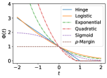
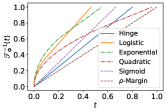
Figure 1: Left: surrogates. Right: ${\mathscr{H}}_{\mathrm{lin}}$-est. error trans. inv.

Definition 3 (${\mathscr{H}}$-estimation error transformation).

The ${\mathscr{H}}$-estimation error transformation of $\Phi$ is defined on $t\in\left[0,1\right]$ by ${\mathscr{T}}_{\Phi}\left(t\right)={\mathscr{T}}(t)\mathds{1}_{t\in\left[\epsilon,1\right]}+({\mathscr{T}}(\epsilon)/\epsilon)\,t\mathds{1}_{t\in\left[0,\epsilon\right)}$, where ${\mathscr{T}}(t):=\inf_{x\in{\mathscr{X}},h\in{\mathscr{H}}:h(x)<0}\Delta{\mathscr{C}}_{\Phi,{\mathscr{H}}}\left(h,x,\frac{t+1}{2}\right)$.

Observe that for any $t\in\left[(1+\epsilon)/2,1\right]$, ${\mathscr{T}}_{\Phi}\left(2t-1\right)=\inf_{x\in{\mathscr{X}},h\in{\mathscr{H}}:h(x)<0}\Delta{\mathscr{C}}_{\Phi,{\mathscr{H}}}(h,x,t)$. Taking $\Psi={\mathscr{T}}_{\Phi}$ satisfies the condition in Theorem 3 if ${\mathscr{T}}_{\Phi}$ is convex with ${\mathscr{T}}_{\Phi}(0)=0$. Moreover, as mentioned earlier, it actually leads to the tightest ${\mathscr{H}}$-consistency estimation error bound (10) when $\epsilon=0$.

Theorem 4 (Tightness).

Suppose that ${\mathscr{H}}$ satisfies the condition of Lemma 1 and that $\epsilon=0$. If ${\mathscr{T}}_{\Phi}$ is convex with ${\mathscr{T}}_{\Phi}(0)=0$, then, for any $t\in[0,1]$ and $\delta>0$, there exist a distribution ${\mathscr{D}}$ and a hypothesis $h\in{\mathscr{H}}$ such that ${\mathscr{R}}_{\ell_{0-1}}(h)-{\mathscr{R}}_{\ell_{0-1},{\mathscr{H}}}^{*}+{\mathscr{M}}_{\ell_{0-1},{\mathscr{H}}}=t$ and ${\mathscr{T}}_{\Phi}(t)\leq{\mathscr{R}}_{\Phi}(h)-{\mathscr{R}}_{\Phi,{\mathscr{H}}}^{*}+{\mathscr{M}}_{\Phi,{\mathscr{H}}}\leq{\mathscr{T}}_{\Phi}(t)+\delta$.

The proof is included in Appendix I. In other words, when $\epsilon=0$, if ${\mathscr{T}}_{\Phi}$ is convex with ${\mathscr{T}}_{\Phi}(0)=0$, it is optimal for the distribution-independent bound (10). Moreover, if ${\mathscr{T}}_{\Phi}$ is additionally invertible and non-increasing, ${\mathscr{T}}_{\Phi}^{-1}$ is the optimal function for the distribution-independent bound in Theorem 12 (Appendix C) and the two bounds are equivalent.

In the following sections, we will see that all these assumptions hold for common loss functions with linear and neural network hypothesis sets. Next, we will apply Theorems 3 and 4 to the linear models (Section 5.3) and neural networks (Section 5.4). Each case requires a detailed analysis (See Appendix K.1 and K.2).

5.3 Linear hypotheses

Table 1: ${\mathscr{H}}_{\mathrm{lin}}$-estimation error transformation and ${\mathscr{H}}_{\mathrm{lin}}$-consistency estimation error bounds with $\epsilon=0$.

Surrogates	${\mathscr{T}}_{\Phi}(t),\,t\in[0,1]$	Bound
Hinge	$\min\left\{B,1\right\}\,t$	(26)
Logistic	$\begin{cases}\frac{t+1}{2}\log_{2}(t+1)+\frac{1-t}{2}\log_{2}(1-t),\quad&t\leq\frac{e^{B}-1}{e^{B}+1},\\ 1-\frac{t+1}{2}\log_{2}(1+e^{-B})-\frac{1-t}{2}\log_{2}(1+e^{B}),\quad&t>\frac{e^{B}-1}{e^{B}+1}.\end{cases}$	(28)
Exponential	$\begin{cases}1-\sqrt{1-t^{2}},&t\leq\frac{e^{2B}-1}{e^{2B}+1},\\ 1-\frac{t+1}{2}e^{-B}-\frac{1-t}{2}e^{B},&t>\frac{e^{2B}-1}{e^{2B}+1}.\end{cases}$	(30)
Quadratic	$\begin{cases}t^{2},&t\leq B,\\ 2B\,t-B^{2},&t>B.\end{cases}$	(32)
Sigmoid	$\tanh(kB)\,t$	(34)
$\rho$-Margin	$\frac{\min\left\{B,\rho\right\}}{\rho}\,t$	(37)

By applying Theorems 3 and 4, we can derive ${\mathscr{H}}_{\mathrm{lin}}$-consistency estimation error bounds for common loss functions defined in Table 2 of Appendix B. Table 1 supplies the ${\mathscr{H}}_{\mathrm{lin}}$-estimation error transformation ${\mathscr{T}}_{\Phi}$ and the corresponding bounds for those loss functions. The inverse ${\mathscr{T}}_{\Phi}^{-1}$ is given in Table 3 of Appendix B. Surrogates $\Phi$ and their corresponding ${\mathscr{T}}_{\Phi}^{-1}$ ($B=0.8$) are visualized in Figure 1. Theorems 3 and 4 apply to all these cases since ${\mathscr{T}}_{\Phi}$ is convex, increasing, invertible and satisfies that ${\mathscr{T}}_{\Phi}(0)=0$. More precisely, taking $\Psi={\mathscr{T}}_{\Phi}$ and $\epsilon=0$ in (10) and using the inverse function ${\mathscr{T}}_{\Phi}^{-1}$ directly give the tightest bound. As an example, for the sigmoid loss, ${\mathscr{T}}_{\Phi_{\mathrm{sig}}}^{-1}(t)=\frac{t}{\tanh(kB)}$. Then the bound (10) becomes ${\mathscr{R}}_{\ell_{0-1}}(h)-{\mathscr{R}}_{\ell_{0-1},{\mathscr{H}}_{\mathrm{lin}}}^{*}\leq({\mathscr{R}}_{\Phi_{\mathrm{sig}}}(h)-{\mathscr{R}}_{\Phi_{\mathrm{sig}},{\mathscr{H}}_{\mathrm{lin}}}^{*}+{\mathscr{M}}_{\Phi_{\mathrm{sig}},{\mathscr{H}}_{\mathrm{lin}}})/\tanh(kB)-{\mathscr{M}}_{\ell_{0-1},{\mathscr{H}}_{\mathrm{lin}}}$, which is (34) in Table 1. Furthermore, after plugging in the minimizability gaps concluded in Table 2, we will obtain the novel bound ${\mathscr{R}}_{\ell_{0-1}}(h)-{\mathscr{R}}_{\ell_{0-1},{\mathscr{H}}_{\mathrm{all}}}^{*}\leq({\mathscr{R}}_{\Phi_{\mathrm{sig}}}(h)-\mathbb{E}_{X}\left[1-\left\lvert 1-2\eta(x)\right\rvert\tanh\left(k\left(W\left\|x\right\|_{p}+B\right)\right)\right])/\tanh(kB)$ ((35) in Appendix K.1.5). The bounds for other surrogates are similarly derived in Appendix K.1. For the logistic loss and exponential loss, to simplify the expression, the bounds are obtained by plugging in an upper bound of ${\mathscr{T}}_{\Phi}^{-1}$.

Let us emphasize that these ${\mathscr{H}}$-consistency estimation error bounds are novel in the sense that they are all hypothesis set-dependent and, to our knowledge, no such guarantee has been presented before. More precisely, the bounds of Table 1 depend directly on the parameter $B$ in the linear models and parameters of the loss function (e.g., $k$ in sigmoid loss). Thus, for a fixed hypothesis $h\in{\mathscr{H}}_{\mathrm{lin}}$, we may give the tightest bound by choosing the best parameter $B$. As an example, Appendix K.1.5 shows that the bound (35) with $B=\plus\infty$ coincides with the excess error bound known for the sigmoid loss (Bartlett et al., 2006). However, for a fixed hypothesis $h$, by varying $B$ (hypothesis set) and $k$ (loss function), we may obtain a finer bound! Thus studying hypothesis set-dependent bounds can guide us to select the most suitable hypothesis set and loss function. Moreover, as shown by Theorem 4, all the bounds obtained by directly using ${\mathscr{T}}_{\Phi}^{-1}$ are tight and cannot be further improved.

5.4 One-hidden-layer ReLU neural networks

In this section, we give ${\mathscr{H}}$-consistency estimation error bounds for one-hidden-layer ReLU neural networks ${\mathscr{H}}_{\mathrm{NN}}$. Table 4 in Appendix B is the counterpart of Table 1 for ${\mathscr{H}}_{\mathrm{NN}}$. Different from the bounds in the linear case, all the bounds in Table 4 not only depend on $B$, but also depend on $\Lambda$, which is a new parameter in ${\mathscr{H}}_{\mathrm{NN}}$. This further illustrates that our bounds are hypothesis set-dependent and, as with the linear case, adequately choosing the parameters $\Lambda$ and $B$ in ${\mathscr{H}}_{\mathrm{NN}}$ would give us better hypothesis set-dependent guarantees than standard excess error bounds. Our proofs and techniques could also be adopted for the analysis of multi-layer neural networks.

5.5 Guarantees under Massart’s noise condition

The distribution-independent ${\mathscr{H}}$-consistency estimation error bound (10) cannot be improved, since they are tight as shown in Theorem 4. However, the bounds can be further improved in the distribution-dependent setting. Indeed, we will study how ${\mathscr{H}}$-consistency estimation error bounds can be improved under low noise conditions, which impose the restrictions on the conditional distribution $\eta(x)$. We consider Massart’s noise condition (Massart & Nédélec, 2006) which is defined as follows.

Definition 4 (Massart’s noise).

The distribution ${\mathscr{D}}$ over $\mathcal{X}\times\mathcal{Y}$ satisfies Massart’s noise condition if $\left\lvert\Delta\eta(x)\right\rvert\geq\beta\text{ for almost all }x\in\mathcal{X}$, for some constant $\beta\in(0,1/2]$.

When it is known that the distribution ${\mathscr{D}}$ satisfies Massart’s noise condition with $\beta$, in contrast with the distribution-independent bounds, we can require the bounds (7) and (9) to hold uniformly only for such distributions. With Massart’s noise condition, we introduce a modified ${\mathscr{H}}$-estimation error transformation in Proposition 1 (Appendix M), which verifies condition (13) of Theorem 8 (the finer distribution dependent guarantee mentioned before, deferred to Appendix C) for all distributions under the noise condition. Then, using this transformation, we can obtain more favorable distribution-dependent bounds. As an example, we consider the quadratic loss $\Phi_{\mathrm{quad}}$, the logistic loss $\Phi_{\mathrm{log}}$ and the exponential loss $\Phi_{\mathrm{exp}}$ with ${\mathscr{H}}_{\mathrm{all}}$. For all distributions and $h\in{\mathscr{H}}_{\mathrm{all}}$, as shown in (Zhang, 2004a; Bartlett et al., 2006; Mohri et al., 2018), the following holds:

$${\mathscr{R}}_{\ell_{0-1}}(h)-{\mathscr{R}}_{\ell_{0-1},{\mathscr{H}}_{\mathrm{all}}}^{*} \leq\sqrt{2}\left({\mathscr{R}}_{\Phi}(h)-{\mathscr{R}}_{\Phi,{\mathscr{H}}_{\mathrm{all}}}^{*}\right)^{1/2},$$

when the surrogate loss $\Phi$ is $\Phi_{\mathrm{log}}$ or $\Phi_{\mathrm{exp}}$. If $\Phi=\Phi_{\mathrm{quad}}$, then the constant multiplier $\sqrt{2}$ can be removed. For distributions that satisfy Massart’s noise condition with $\beta$, as proven in Appendix M, for any $h\in{\mathscr{H}}_{\mathrm{all}}$ such that ${\mathscr{R}}_{\Phi}(h)\leq{\mathscr{R}}_{\Phi,{\mathscr{H}}_{\mathrm{all}}}^{*}+{\mathscr{T}}(2\beta)$, the consistency excess error bound is improved from the square-root dependency to a linear dependency:

$$\mspace{-14.0mu}{\mathscr{R}}_{\ell_{0-1}}(h)-{\mathscr{R}}_{\ell_{0-1},{\mathscr{H}}_{\mathrm{all}}}^{*}\mspace{-2.0mu}\leq\mspace{-2.0mu}2\beta\left({\mathscr{R}}_{\Phi}(h)-{\mathscr{R}}_{\Phi,{\mathscr{H}}_{\mathrm{all}}}^{*}\right)/{\mathscr{T}}(2\beta),\mspace{-8.0mu}$$ (11)

where ${\mathscr{T}}(t)$ equals to $t^{2}$, $\frac{t+1}{2}\log_{2}(t+1)+\frac{1-t}{2}\log_{2}(1-t)$ and $1-\sqrt{1-t^{2}}$ for $\Phi_{\mathrm{quad}}$, $\Phi_{\mathrm{log}}$ and $\Phi_{\mathrm{exp}}$ respectively. These linear dependent bounds are tight, as illustrated in Section 7.

6 Guarantees for the adversarial loss $\ell_{2}=\ell_{\gamma}$

In this section, we discuss the adversarial scenario where $\ell_{2}$ is the adversarial $0/1$ loss $\ell_{\gamma}$. We consider symmetric hypothesis sets, which satisfy: $h\in{\mathscr{H}}$ if and only if $-h\in{\mathscr{H}}$. For convenience, we will adopt the following definitions:

$$\underline{h}_{\gamma}(x)=\inf_{x^{\prime}\colon\|x-x^{\prime}\|_{p}\leq\gamma}h(x^{\prime})\qquad\overline{h}_{\gamma}(x)=\sup_{x^{\prime}\colon\|x-x^{\prime}\|_{p}\leq\gamma}h(x^{\prime}).$$

We also define $\overline{\mathscr{H}}_{\gamma}=\left\{h\in{\mathscr{H}}:\underline{h}_{\gamma}(x)\leq 0\leq\overline{h}_{\gamma}(x)\right\}$. The following characterization of the minimal conditional $\ell_{\gamma}$-risk and conditional $\epsilon$-regret is based on (Awasthi et al., 2021a, Lemma 27) and will be helpful in introducing the general tools in Section 6.1. The proof is similar and is included in Appendix E for completeness.

Lemma 2.

Assume that ${\mathscr{H}}$ is symmetric. Then, the minimal conditional $\ell_{\gamma}$-risk is

$${\mathscr{C}}^{*}_{\ell_{\gamma},{\mathscr{H}}}(x)=\min\left\{\eta(x),1-\eta(x)\right\}\mathds{1}_{\overline{\mathscr{H}}_{\gamma}\neq{\mathscr{H}}}+\mathds{1}_{\overline{\mathscr{H}}_{\gamma}={\mathscr{H}}}\,.$$

The conditional $\epsilon$-regret for $\ell_{\gamma}$ can be characterized as

$$\left\langle\Delta{\mathscr{C}}_{\ell_{\gamma},{\mathscr{H}}}(h,x)\right\rangle_{\epsilon}=\begin{cases}\left\langle\left\lvert\Delta\eta(x)\right\rvert+\frac{1}{2}\right\rangle_{\epsilon}&h\in\overline{\mathscr{H}}_{\gamma}\subsetneqq{\mathscr{H}}\\ \left\langle 2\Delta\eta(x)\right\rangle_{\epsilon}&\overline{h}_{\gamma}(x)<0\\ \left\langle-2\Delta\eta(x)\right\rangle_{\epsilon}&\underline{h}_{\gamma}(x)>0\\ 0&\text{otherwise}\end{cases}$$

6.1 General hypothesis sets ${\mathscr{H}}$

As with the non-adversarial case, we begin by providing general theoretical tools to study ${\mathscr{H}}$-consistency estimation error bounds when the target loss is the adversarial $0/1$ loss. Lemma 2 characterizes the conditional $\epsilon$-regret for $\ell_{\gamma}$ with symmetric hypothesis sets. Thus, Theorems 1 and 2 can be instantiated as Theorems 10 and 11 (See Appendix C) in these cases. These results are distribution-dependent and can serve as general tools. For example, we can use these tools to derive more favorable guarantees under noise conditions (Section 6.5). As in the previous section, we present their distribution-independent version in the following theorem.

Theorem 5 (Adversarial distribution-independent $\Psi$-bound).

Suppose that ${\mathscr{H}}$ is symmetric. Assume there exist a convex function $\Psi\colon\mathbb{R_{+}}\to\mathbb{R}$ with $\Psi(0)=0$ and $\epsilon\geq 0$ such that the following holds for any $t\in\left[1/2,1\right]\colon$

$$\Psi\left(\left\langle t\right\rangle_{\epsilon}\right)\leq\inf_{x\in{\mathscr{X}},h\in\overline{\mathscr{H}}_{\gamma}\subsetneqq{\mathscr{H}}}\Delta{\mathscr{C}}_{\widetilde{\Phi},{\mathscr{H}}}(h,x,t),$$

$$\Psi\left(\left\langle 2t-1\right\rangle_{\epsilon}\right)\leq\inf_{x\in{\mathscr{X}},h\in{\mathscr{H}}\colon\overline{h}_{\gamma}(x)<0}\Delta{\mathscr{C}}_{\widetilde{\Phi},{\mathscr{H}}}(h,x,t).$$

Then, for any hypothesis $h\in{\mathscr{H}}$ and any distribution,

$$\Psi\left({\mathscr{R}}_{\ell_{\gamma}}(h)-{\mathscr{R}}_{\ell_{\gamma},{\mathscr{H}}}^{*}+{\mathscr{M}}_{\ell_{\gamma},{\mathscr{H}}}\right)\leq{\mathscr{R}}_{\widetilde{\Phi}}(h)-{\mathscr{R}}_{\widetilde{\Phi},{\mathscr{H}}}^{*}+{\mathscr{M}}_{\widetilde{\Phi},{\mathscr{H}}}+\max\left\{0,\Psi(\epsilon)\right\}.$$ (12)

The counterpart of Theorem 5 is Theorem 13 (adversarial distribution-independent $\Gamma$-bound), deferred to Appendix C due to space limitations. The proofs for both theorems are included in Appendix H. As with the non-adversarial scenario, the tightest distribution-independent ${\mathscr{H}}$-consistency estimation error bounds obtained by Theorem 5 can be achieved by the optimal $\Psi$, which is the adversarial ${\mathscr{H}}$-estimation error transformation defined as follows.

Definition 5 (Adversarial ${\mathscr{H}}$-estimation error transformation).

The adversarial ${\mathscr{H}}$-estimation error transformation of $\widetilde{\Phi}$ is defined on $t\in\left[0,1\right]$ by ${\mathscr{T}}_{\widetilde{\Phi}}\left(t\right)=\min\left\{{\mathscr{T}}_{1}(t),{\mathscr{T}}_{2}(t)\right\}$,

where $${\mathscr{T}}_{1}(t):=\widehat{{\mathscr{T}}}_{1}(t)\mathds{1}_{t\in[1/2,1]}+2\,\widehat{{\mathscr{T}}}_{1}(1/2)\,t\mathds{1}_{t\in[0,1/2)},$$

$${\mathscr{T}}_{2}(t):=\widehat{{\mathscr{T}}}_{2}(t)\mathds{1}_{t\in\left[\epsilon,1\right]}+\big{(}\widehat{{\mathscr{T}}}_{2}(\epsilon)/\epsilon\big{)}\,t\mathds{1}_{t\in\left[0,\epsilon\right)},$$

with $$\widehat{{\mathscr{T}}}_{1}(t):=\inf_{x\in{\mathscr{X}},h\in\overline{\mathscr{H}}_{\gamma}\subsetneqq{\mathscr{H}}}\Delta{\mathscr{C}}_{\widetilde{\Phi},{\mathscr{H}}}(h,x,t),$$

$$\widehat{{\mathscr{T}}}_{2}(t):=\inf_{x\in{\mathscr{X}},h\in{\mathscr{H}}\colon\overline{h}_{\gamma}(x)<0}\Delta{\mathscr{C}}_{\widetilde{\Phi},{\mathscr{H}}}\big{(}h,x,\frac{t+1}{2}\big{)}.$$

It is clear that ${\mathscr{T}}_{\widetilde{\Phi}}$ satisfies assumptions in Theorem 5. The next theorem shows that it gives the tightest ${\mathscr{H}}$-consistency estimation error bound (12) under certain conditions.

Theorem 6 (Adversarial tightness).

Suppose that ${\mathscr{H}}$ is symmetric and that $\epsilon=0$. If ${\mathscr{T}}_{\widetilde{\Phi}}=\min\left\{{\mathscr{T}}_{1},{\mathscr{T}}_{2}\right\}$ is convex with ${\mathscr{T}}_{\widetilde{\Phi}}(0)=0$ and ${\mathscr{T}}_{2}\leq{\mathscr{T}}_{1}$, then, for any $t\in[0,1]$ and $\delta>0$, there exist a distribution ${\mathscr{D}}$ and a hypothesis $h\in{\mathscr{H}}$ such that ${\mathscr{R}}_{\ell_{\gamma}}(h)-{\mathscr{R}}_{\ell_{\gamma},{\mathscr{H}}}^{*}+{\mathscr{M}}_{\ell_{\gamma},{\mathscr{H}}}=t$ and ${\mathscr{T}}_{\widetilde{\Phi}}(t)\leq{\mathscr{R}}_{\widetilde{\Phi}}(h)-{\mathscr{R}}_{\widetilde{\Phi},{\mathscr{H}}}^{*}+{\mathscr{M}}_{\widetilde{\Phi},{\mathscr{H}}}\leq{\mathscr{T}}_{\widetilde{\Phi}}(t)+\delta$.

The proof is included in Appendix I. In other words, when $\epsilon=0$, if ${\mathscr{T}}_{2}\leq{\mathscr{T}}_{1}$ and ${\mathscr{T}}_{\widetilde{\Phi}}$ is convex with ${\mathscr{T}}_{\widetilde{\Phi}}(0)=0$, ${\mathscr{T}}_{\widetilde{\Phi}}$ is the optimal function for the distribution-independent bound (12). Moreover, if ${\mathscr{T}}_{\widetilde{\Phi}}$ is additionally invertible and non-increasing, ${\mathscr{T}}_{\widetilde{\Phi}}^{-1}$ is the optimal function for the distribution-independent bound in Theorem 13 (Appendix C) and the two bounds will be equivalent.

We will see that all these assumptions hold for cases considered in Section 6.3 and 6.4. Next, we will apply Theorem 5 along with the tightness guarantee Theorem 6 to study specific hypothesis sets and adversarial surrogate loss functions in Section 6.2 for negative results and Section 6.3 and 6.4 for positive results. A careful analysis is presented in each case (See Appendix L).

6.2 Negative results for adversarial robustness

Awasthi et al. (2021a) show that supremum-based convex loss functions of the type $\widetilde{\Phi}=\sup_{x^{\prime}\colon\|x-x^{\prime}\|_{p}\leq\gamma}\Phi(yh(x^{\prime}))$, where $\Phi$ is convex and non-increasing, are not ${\mathscr{H}}$-calibrated with respect to $\ell_{\gamma}$ for ${\mathscr{H}}$ containing 0, that is regular for adversarial calibration (Definition 6 in Appendix J), e.g., ${\mathscr{H}}_{\mathrm{lin}}$ and ${\mathscr{H}}_{\mathrm{NN}}$. Similarly, we show that there are no non-trivial adversarial ${\mathscr{H}}$-consistency estimation error bounds with respect to $\ell_{\gamma}$ for supremum-based convex loss functions and supremum-based sigmoid loss with such hypothesis sets. Note that Awasthi et al. (2021a) do not study the sigmoid loss, which is non-convex. Thus, our results go beyond their results for convex adversarial surrogates.

Theorem 7 (Negative results for robustness).

Suppose that ${\mathscr{H}}$ contains $0$ and is regular for adversarial calibration. Let $\ell_{1}$ be supremum-based convex loss or supremum-based sigmoid loss and $\ell_{2}=\ell_{\gamma}$. Then, $f\geq 1/2$ are the only non-decreasing functions $f$ such that (3) holds.

The proof is given in Appendix J. In other words, the function $f$ in bound (3) must be lower bounded by $1/2$ for such adversarial surrogates. Theorem 7 implies that the loss functions commonly used in practice for optimizing the adversarial loss cannot benefit from any useful ${\mathscr{H}}$-consistency estimation error guarantees. Instead, we show in Section 6.3 and 6.4 that the supremum-based $\rho$-margin loss $\widetilde{\Phi}_{\rho}=\sup_{x^{\prime}\colon\|x-x^{\prime}\|_{p}\leq\gamma}\Phi_{\mathrm{\rho}}(yh(x^{\prime}))$ proposed by (Awasthi et al., 2021a) admits favorable adversarial ${\mathscr{H}}$-consistency estimation error bounds. These bounds would also imply significantly stronger results than the asymptotic ${\mathscr{H}}$-consistency guarantee in (Awasthi et al., 2021a).

6.3 Linear hypotheses

In this section, by applying Theorems 10 and 11, we derive the adversarial ${\mathscr{H}}_{\mathrm{lin}}$-consistency estimation error bound (54) in Table 5 of Appendix B for supremum-based $\rho$-margin loss. This is a completely new consistency estimation error bound in the adversarial setting. As with the non-adversarial case, the bound is dependent on the parameter $B$ in linear hypothesis set and $\rho$ in the loss function. This helps guide the choice of loss functions once the hypothesis set is fixed. More precisely, if $B>0$ is known, we can always choose $\rho<B$ such that the bound is the tightest. Moreover, the bound can turn into more significant $\epsilon$-consistency results in adversarial setting than the ${\mathscr{H}}$-consistency result in (Awasthi et al., 2021a).

Corollary 3.

Let ${\mathscr{D}}$ be a distribution over ${\mathscr{X}}\times{\mathscr{Y}}$ such that ${\mathscr{M}}_{\widetilde{\Phi}_{\rho},{\mathscr{H}}_{\mathrm{lin}}}\leq\epsilon$ for some $\epsilon\geq 0$. Then, the following holds:

$$\mspace{-3.0mu}{\mathscr{R}}_{\ell_{\gamma}}\mspace{-3.0mu}(h)\mspace{-1.0mu}-\mspace{-1.0mu}{\mathscr{R}}_{\ell_{\gamma},{\mathscr{H}}_{\mathrm{lin}}}^{*}\mspace{-4.0mu}\leq\mspace{-4.0mu}\rho\left({\mathscr{R}}_{\widetilde{\Phi}_{\rho}}\mspace{-3.0mu}(h)\mspace{-1.0mu}-\mspace{-1.0mu}{\mathscr{R}}_{\widetilde{\Phi}_{\rho},{\mathscr{H}}_{\mathrm{lin}}}^{*}\mspace{-1.0mu}+\mspace{-1.0mu}\epsilon\right)/\min\left\{B,\rho\right\}.$$

Awasthi et al. (2021a) show that $\widetilde{\Phi}_{\rho}$ is ${\mathscr{H}}_{\mathrm{lin}}$-consistent with respect to $\ell_{\gamma}$ when ${\mathscr{M}}_{\widetilde{\Phi}_{\rho},{\mathscr{H}}_{\mathrm{lin}}}=0$. This result can be immediately implied by Corollary 3. Moreover, Corollary 3 provides guarantees for more general cases where ${\mathscr{M}}_{\widetilde{\Phi}_{\rho},{\mathscr{H}}_{\mathrm{lin}}}$ can be nonzero.

6.4 One-hidden-layer ReLU neural networks

For the one-hidden-layer ReLU neural networks ${\mathscr{H}}_{\mathrm{NN}}$ and $\widetilde{\Phi}_{\rho}$, we have the ${\mathscr{H}}_{\mathrm{NN}}$-estimation error bound (59) in Table 5. Note $\inf_{x\in{\mathscr{X}}}\sup_{h\in{\mathscr{H}}_{\mathrm{NN}}}\underline{h}_{\gamma}(x)$ does not have an explicit expression. However, (59) can be further relaxed to be (60) in Appendix L.2, which is identical to the bound in the linear case modulo the replacement of $B$ by $\Lambda B$. As in the linear case, the bound is new and also implies stronger $\epsilon$-consistency results as follows:

Corollary 4.

Let ${\mathscr{D}}$ be a distribution over ${\mathscr{X}}\times{\mathscr{Y}}$ such that ${\mathscr{M}}_{\widetilde{\Phi}_{\rho},{\mathscr{H}}_{\mathrm{NN}}}\leq\epsilon$ for some $\epsilon\geq 0$. Then,

$$\mspace{-6.0mu}{\mathscr{R}}_{\ell_{\gamma}}\mspace{-3.0mu}(h)\mspace{-1.0mu}-\mspace{-1.0mu}{\mathscr{R}}_{\ell_{\gamma},{\mathscr{H}}_{\mathrm{NN}}}^{*}\mspace{-4.0mu}\leq\mspace{-4.0mu}\rho\left({\mathscr{R}}_{\widetilde{\Phi}_{\rho}}\mspace{-3.0mu}(h)\mspace{-1.0mu}-\mspace{-1.0mu}{\mathscr{R}}_{\widetilde{\Phi}_{\rho},{\mathscr{H}}_{\mathrm{NN}}}^{*}\mspace{-10.0mu}+\mspace{-4.0mu}\epsilon\right)\mspace{-1.0mu}/\mspace{-5.0mu}\min\left\{\Lambda B,\rho\right\}\mspace{-4.0mu}.$$

Besides the bounds for $\widetilde{\Phi}_{\rho}$, Table 5 gives a series of results that are all new in the adversarial setting. Like the bounds in Table 1 and 4, they are all hypothesis set dependent and very useful. For example, the improved bounds for $\widetilde{\Phi}_{\mathrm{hinge}}$ and $\widetilde{\Phi}_{\mathrm{sig}}$ under noise conditions in the table can also turn into meaningful consistency results under Massart’s noise condition, as shown in Section 6.5.

6.5 Guarantees under Massart’s noise condition

Section 6.2 shows that non-trivial distribution-independent bounds for supremum-based hinge loss and supremum-based sigmoid loss do not exist. However, under Massart’s noise condition (Definition 4), we will show that there exist non-trivial adversarial ${\mathscr{H}}$-consistency estimation error bounds for the two loss functions. Furthermore, we will see that the bounds are linear dependent as those in Section 5.5.

As with the non-adversarial scenario, we introduce a modified adversarial ${\mathscr{H}}$-estimation error transformation in Proposition 2 (Appendix N). Using this tool, we derive adversarial ${\mathscr{H}}$-consistency estimation error bounds for $\widetilde{\Phi}_{\mathrm{hinge}}$ and $\widetilde{\Phi}_{\mathrm{sig}}$ under Massart’s noise condition in Table 5. From the bounds (67), (69), (71), and (73), we can also obtain novel $\epsilon$-consistency results for $\widetilde{\Phi}_{\mathrm{hinge}}$ and $\widetilde{\Phi}_{\mathrm{sig}}$ with linear models and neural networks under Massart’s noise condition.

Corollary 5.

Let ${\mathscr{H}}$ be ${\mathscr{H}}_{\mathrm{lin}}$ or ${\mathscr{H}}_{\mathrm{NN}}$. Let ${\mathscr{D}}$ be a distribution over ${\mathscr{X}}\times{\mathscr{Y}}$ which satisfies Massart’s noise condition with $\beta$ such that ${\mathscr{M}}_{\widetilde{\Phi},{\mathscr{H}}}\leq\epsilon$ for some $\epsilon\geq 0$. Then,

$${\mathscr{R}}_{\ell_{\gamma}}(h)-{\mathscr{R}}_{\ell_{\gamma},{\mathscr{H}}}^{*}\leq\frac{1+2\beta}{4\beta}({\mathscr{R}}_{\widetilde{\Phi}}(h)-{\mathscr{R}}_{\widetilde{\Phi},{\mathscr{H}}}^{*}+\epsilon)/{\mathscr{T}}(B),$$

where ${\mathscr{T}}(t)$ equals to $\min\left\{t,1\right\}$ and $\tanh\left(kt\right)$ for $\widetilde{\Phi}_{\mathrm{hinge}}$ and $\widetilde{\Phi}_{\mathrm{sig}}$ respectively, $B$ is replaced by $\Lambda B$ for ${\mathscr{H}}={\mathscr{H}}_{\mathrm{NN}}$.

In Section 7, we will further show that these linear dependency bounds in adversarial setting are tight, along with the non-adversarial bounds we discussed earlier in Section 5.5.

7 Simulations

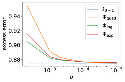
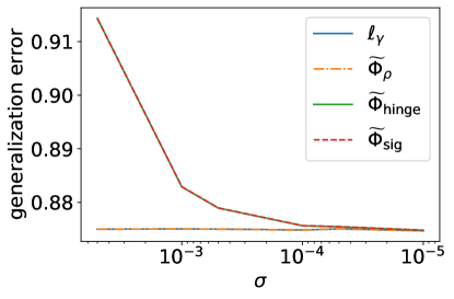
Figure 2: Left: tightness of bound (11) in Section 5.5. Right: tightness of bound (54),(67) and (69) in Section 6.3 and 6.5.

Here, we present experiments on simulated data to illustrate our bounds and their tightness. We generate data points $x\in\mathbb{R}$ on $[-1,+1]$. All risks are approximated by their empirical counterparts computed over $10^{7}$ i.i.d. samples.

Non-adversarial. To demonstrate the tightness of our non-adversarial bounds, we consider a scenario where the marginal distribution is symmetric about $x=0$ with labels flipped. With probability $\frac{1}{16}$, $(x,y)=(1,-1)$; with probability $\frac{7}{16}$, the label is $+1$ and the data follows the truncated normal distribution on $[\sigma,1]$ with both mean and standard deviation $\sigma$. We consider $\Phi_{\mathrm{quad}}$, $\Phi_{\mathrm{log}}$ and $\Phi_{\mathrm{exp}}$ defined in Table 2 of Appendix B. The distribution considered satisfies Massart’s noise condition with $\beta=\frac{1}{2}$. Thus, our bound (11) in Section 5.5 becomes ${\mathscr{R}}_{\ell_{0-1}}(h)-{\mathscr{R}}_{\ell_{0-1},{\mathscr{H}}_{\mathrm{all}}}^{*}\leq{\mathscr{R}}_{\Phi}(h)-{\mathscr{R}}_{\Phi,{\mathscr{H}}_{\mathrm{all}}}^{*}$, for any $h\in{\mathscr{H}}_{\mathrm{all}}$ such that ${\mathscr{R}}_{\Phi}(h)\leq{\mathscr{R}}_{\Phi,{\mathscr{H}}_{\mathrm{all}}}^{*}+1$. All the minimal generalization errors vanish in this case. As shown in Figure 2, for $h(x)=-5x$, the bounds corresponding to $\Phi_{\mathrm{quad}}$, $\Phi_{\mathrm{log}}$ and $\Phi_{\mathrm{exp}}$ are all tight as $\sigma\to 0$.

Adversarial. To demonstrate the tightness of our adversarial bounds, the distribution is modified as follows: with probability $\frac{1}{16}$, $(x,y)=(1,-1)$; with probability $\frac{1}{16}$, $(x,y)=(-1,+1)$; with probability $\frac{7}{8}$, the label is $-1$ and the data follows the truncated normal distribution on $[-1,\gamma-\sigma]$ with mean $\gamma-\sigma$ and standard deviation $\sigma$. We set $\gamma=0.1$ and consider $\widetilde{\Phi}_{\rho}$ with $\rho=1$, $\widetilde{\Phi}_{\mathrm{hinge}}$ and $\widetilde{\Phi}_{\mathrm{sig}}$ with $k=1$. The distribution considered satisfies Massart’s noise condition with $\beta=\frac{1}{2}$. Thus, our bounds (54), (67) and (69) in Table 5 become ${\mathscr{R}}_{\ell_{\gamma}}(h)\leq{\mathscr{R}}_{\ \widetilde{\Phi}}(h)$, for any $h\in{\mathscr{H}}_{\mathrm{lin}}$. As shown in Figure 2, for $h(x)=-5x$, the bounds corresponding to $\widetilde{\Phi}_{\rho}$, $\widetilde{\Phi}_{\mathrm{hinge}}$ and $\widetilde{\Phi}_{\mathrm{sig}}$ are all tight as $\sigma\to 0$.

8 Conclusion

We presented an exhaustive study of ${\mathscr{H}}$-consistency estimation error bounds, including a series of new guarantees for both the non-adversarial zero-one loss function and the adversarial zero-one loss function. Our hypothesis-dependent guarantees are significantly stronger than the consistency or calibration ones. Our results include a series of theoretical and conceptual tools helpful for the analysis of other loss functions and other hypothesis sets, including multi-class classification or ranking losses.

Appendix A Related Work

Bayes-consistency (also known as consistency) and excess error bounds between margin-based loss functions and the zero-one loss have been widely studied in the literature (Zhang, 2004a; Bartlett et al., 2006; Steinwart, 2007; Mohri et al., 2018). Consistency studies the asymptotic relation between the surrogate excess error and the target excess error while excess error bounds study the quantitative relation between them and thus is stronger. They both consider the hypothesis set of all measurable functions. The works of Zhang (2004a), Bartlett et al. (2006), and Steinwart (2007) studied consistency via the lens of calibration and showed that calibration and consistency are equivalent in the standard binary classification when considering the hypothesis set of all measurable functions.

The work of Zhang (2004a) analyzed how close to the optimal excess error of the zero-one loss can one reach via minimizers of convex surrogates. Bartlett et al. (2006) extended the results in (Zhang, 2004a) and developed a general methodology for finding quantitative bounds between the excess error associated with the zero-one loss and the excess error of margin-based surrogate loss functions for all distributions. In a recent work, Mohri et al. (2018) simplified these results and provided different proofs for the excess error bounds of various loss functions widely used in practice. Calibration and consistency analysis have also been extended to multi-class settings (Zhang, 2004b; Tewari & Bartlett, 2007) and to ranking problems (Uematsu & Lee, 2011; Gao & Zhou, 2015).

Bayes-consistency is not an appropriate notion when studying learning with a hypothesis set ${\mathscr{H}}$ that is distinct from the family of all measurable functions. Therefore, a new hypothesis set-dependent notion namely, ${\mathscr{H}}$-consistency, has been proposed and explored in the more recent literature (Long & Servedio, 2013; Kuznetsov et al., 2014; Zhang & Agarwal, 2020). In particular, Long & Servedio (2013) argued that ${\mathscr{H}}$-consistency is a more useful notion than consistency by empirically showing that certain loss functions that are ${\mathscr{H}}$-consistent but not Bayes consistent can perform significantly better than a loss function known to be Bayes consistent. The work of Kuznetsov et al. (2014) extended the ${\mathscr{H}}$-consistency results in (Long & Servedio, 2013) to the case of structured prediction and provided positive results for ${\mathscr{H}}$-consistency of several multi-class ensemble algorithms.

In a recent work Zhang & Agarwal (2020) investigated the empirical phenomenon in (Long & Servedio, 2013) and designed a class of piecewise linear scoring functions such that minimizing a surrogate that is not ${\mathscr{H}}$-consistent over this larger class yields ${\mathscr{H}}$-consistency of linear models. For linear predictors, more general margin-based properties of convex surrogate losses are also studied in (Long & Servedio, 2011; Ben-David et al., 2012). Aiming for such margin based error guarantees, Ben-David et al. (2012) argued that the hinge loss is optimal among convex losses.

Most recently, the notion of ${\mathscr{H}}$-consistency along with ${\mathscr{H}}$-calibration have also been studied in the context of adversarially robust classification (Bao et al., 2021; Awasthi et al., 2021a). In the adversarial scenario, in contrast to standard classification, the target loss is the adversarial zero-one loss (Goodfellow et al., 2014; Madry et al., 2017; Carlini & Wagner, 2017; Tsipras et al., 2018; Shafahi et al., 2019; Wong et al., 2020). This corresponds to the worst zero-one loss incurred over an adversarial perturbation of $x$ within a $\gamma$-ball as measured in a norm, typically $\ell_{p}$ for $p\in[1,\plus\infty]$. The adversarial loss presents new challenges and makes the consistency analysis significantly more complex.

The work of Bao et al. (2021) initiated the study of ${\mathscr{H}}$-calibration with respect to the adversarial zero-one loss for the linear models. They showed that convex surrogates are not calibrated and introduced a class of nonconvex margin-based surrogate losses. They then provided sufficient conditions for such nonconvex losses to be calibrated in the linear case. The work of Awasthi et al. (2021a) extended the results in (Bao et al., 2021) to the general nonlinear hypothesis sets and pointed out that although ${\mathscr{H}}$-calibration is a necessary condition of ${\mathscr{H}}$-consistency, it is not sufficient in the adversarial scenario. They then proposed sufficient conditions which guarantee calibrated losses to be consistent in the setting of adversarially robust classification.

All the above mentioned works either studied asymptotic properties (Bayes-consistency or ${\mathscr{H}}$-consistency) or studied quantitative relations when ${\mathscr{H}}$ is the family of all measurable functions (excess error bounds). Instead, our work considers a hypothesis set-dependent quantitative relation between the surrogate estimation error and the target estimation error. This is significantly stronger than ${\mathscr{H}}$-calibration or ${\mathscr{H}}$-consistency and is also more informative than excess error bounds which correspond to a special case of our results with ${\mathscr{H}}={\mathscr{H}}_{\mathrm{all}}$. As a by-product, our theory contributes more significant consistency results for the poorly understood setting of adversarial robustness. There have also been recent works on different theoretical aspects of adversarial robustness such as tension between the zero-one loss and the adversarial zero-one loss (Tsipras et al., 2018; Zhang et al., 2019), computational bottlenecks for adversarial loss (Bubeck et al., 2018a, b; Awasthi et al., 2019), adversarial examples (Bartlett et al., 2021; Bubeck et al., 2021), sample complexity of adversarial surrogate losses (Khim & Loh, 2018; Cullina et al., 2018; Yin et al., 2019; Montasser et al., 2019; Awasthi et al., 2020), computational complexity of adversarially robust linear classifiers (Diakonikolas et al., 2020), connections with PAC learning (Montasser et al., 2020; Viallard et al., 2021), perturbations beyond $\ell_{p}$ norm(Feige et al., 2015, 2018; Attias et al., 2018), adversarial robustness optimization (Robey et al., 2021), overparametrization (Bubeck & Sellke, 2021) and Bayes optimality (Awasthi et al., 2021b).

Appendix B Deferred Tables

Table 2: Loss functions and their minimizability gaps. In some cases, the minimizability gap coincides with the approximation error. For example, ${\mathscr{M}}_{\Phi_{\mathrm{sig}},{\mathscr{H}}_{\mathrm{lin}}}={\mathscr{R}}_{\Phi_{\mathrm{sig}},{\mathscr{H}}_{\mathrm{lin}}}^{*}-\mathbb{E}_{X}\left[1-\left\lvert 1-2\eta(x)\right\rvert\tanh\left(k\left(W\left\|x\right\|_{p}+B\right)\right)\right]$ coincides with the $\left(\Phi_{\mathrm{sig}},{\mathscr{H}}_{\mathrm{lin}}\right)$-approximation error ${\mathscr{R}}_{\Phi_{\mathrm{sig}},{\mathscr{H}}_{\mathrm{lin}}}^{*}-\mathbb{E}_{X}\left[1-\left\lvert 1-2\eta(x)\right\rvert\right]$ for $B=\plus\infty$; ${\mathscr{M}}_{\Phi_{\mathrm{hinge}},{\mathscr{H}}_{\mathrm{NN}}}={\mathscr{R}}_{\Phi_{\mathrm{hinge}},{\mathscr{H}}_{\mathrm{NN}}}^{*}-\mathbb{E}_{X}\left[1-\left\lvert 2\eta(x)-1\right\rvert\min\left\{\Lambda W\left\|x\right\|_{p}+\Lambda B,1\right\}\right]$ coincides with the $\left(\Phi_{\mathrm{hinge}},{\mathscr{H}}_{\mathrm{NN}}\right)$-approximation error ${\mathscr{R}}_{\Phi_{\mathrm{hinge}},{\mathscr{H}}_{\mathrm{NN}}}^{*}-\mathbb{E}_{X}\left[1-\left\lvert 1-2\eta(x)\right\rvert\right]$ for $\Lambda B\geq 1$. The detailed derivation is included in Appendix K, L.

Loss Functions	Definitions	${\mathscr{M}}_{\ell,{\mathscr{H}}_{\mathrm{lin}}}$	${\mathscr{M}}_{\ell,{\mathscr{H}}_{\mathrm{NN}}}$
Hinge	$\Phi_{\mathrm{hinge}}(t)=\max\left\{0,1-t\right\}$	(25)	(40)
Logistic	$\Phi_{\mathrm{log}}(t)=\log_{2}(1+e^{-t})$	(27)	(42)
Exponential	$\Phi_{\mathrm{exp}}(t)=e^{-t}$	(29)	(44)
Quadratic	$\Phi_{\mathrm{quad}}(t)=(1-t)^{2}\mathds{1}_{t\leq 1}$	(31)	(31)
Sigmoid	$\Phi_{\mathrm{sig}}(t)=1-\tanh(kt),~{}k>0$	(33)	(48)
$\rho$-Margin	$\Phi_{\rho}(t)=\min\left\{1,\max\left\{0,1-\frac{t}{\rho}\right\}\right\},~{}\rho>0$	(36)	(40)
Sup-$\rho$-Margin	$\widetilde{\Phi}_{\rho}=\sup_{x^{\prime}\colon\|x-x^{\prime}\|_{p}\leq\gamma}\Phi_{\rho}(yh(x^{\prime}))$	(53)	(58)
Zero-One	$\ell_{0-1}=\mathds{1}_{\operatorname{sign}(h(x))\neq y}$	(24)	(39)
Adversarial Zero-One	$\ell_{\gamma}=\sup_{x^{\prime}\colon\|x-x^{\prime}\|_{p}\leq\gamma}\mathds{1}_{yh(x^{\prime})\leq 0}$	(52)	(57)

Table 3: Non-adversarial ${\mathscr{H}}_{\mathrm{lin}}$-estimation error transformation ($\epsilon=0)$ and ${\mathscr{H}}_{\mathrm{lin}}$-consistency estimation error bounds. All the bounds are hypothesis set-dependent (parameter $B$ in ${\mathscr{H}}_{\mathrm{lin}}$) and provide novel guarantees as discussed in Section 5.3. The minimizability gaps appearing in the bounds for the surrogates are concluded in Table 2. The detailed derivation is included in Appendix K.1.

Surrogates	${\mathscr{T}}_{\Phi}(t),\,t\in[0,1]$	${\mathscr{T}}_{\Phi}^{-1}(t),\,t\in\mathbb{R}_{+}$	Bound
Hinge	$\min\left\{B,1\right\}\,t$	$\frac{t}{\min\left\{B,1\right\}}$	(26)
Logistic	$\begin{cases}\frac{t+1}{2}\log_{2}(t+1)+\frac{1-t}{2}\log_{2}(1-t),\quad&t\leq\frac{e^{B}-1}{e^{B}+1},\\ 1-\frac{t+1}{2}\log_{2}(1+e^{-B})-\frac{1-t}{2}\log_{2}(1+e^{B}),\quad&t>\frac{e^{B}-1}{e^{B}+1}.\end{cases}$	upper bounded by $\begin{cases}\sqrt{2t},&t\leq\frac{1}{2}\left(\frac{e^{B}-1}{e^{B}+1}\right)^{2},\\ 2\left(\frac{e^{B}+1}{e^{B}-1}\right)\,t,&t>\frac{1}{2}\left(\frac{e^{B}-1}{e^{B}+1}\right)^{2}.\end{cases}$	(28)
Exponential	$\begin{cases}1-\sqrt{1-t^{2}},&t\leq\frac{e^{2B}-1}{e^{2B}+1},\\ 1-\frac{t+1}{2}e^{-B}-\frac{1-t}{2}e^{B},&t>\frac{e^{2B}-1}{e^{2B}+1}.\end{cases}$	upper bounded by $\begin{cases}\sqrt{2t},&t\leq\frac{1}{2}\left(\frac{e^{2B}-1}{e^{2B}+1}\right)^{2},\\ 2\left(\frac{e^{2B}+1}{e^{2B}-1}\right)\,t,&t>\frac{1}{2}\left(\frac{e^{2B}-1}{e^{2B}+1}\right)^{2}.\end{cases}$	(30)
Quadratic	$\begin{cases}t^{2},&t\leq B,\\ 2B\,t-B^{2},&t>B.\end{cases}$	$\begin{cases}\sqrt{t},&t\leq B^{2},\\ \frac{t}{2B}+\frac{B}{2},&t>B^{2}.\end{cases}$	(32)
Sigmoid	$\tanh(kB)\,t$	$\frac{t}{\tanh(kB)}$	(34)
$\rho$-Margin	$\frac{\min\left\{B,\rho\right\}}{\rho}\,t$	$\frac{\rho}{\min\left\{B,\rho\right\}}\,t$	(37)

Table 4: Non-adversarial ${\mathscr{H}}_{\mathrm{NN}}$-estimation error transformation ($\epsilon=0)$ and ${\mathscr{H}}_{\mathrm{NN}}$-consistency estimation error bounds. All the bounds are hypothesis set-dependent (parameter $\Lambda$ and $B$ in ${\mathscr{H}}_{\mathrm{NN}}$) and provide novel guarantees as dicussed in Section 5.4. The minimizability gaps appearing in the bounds for the surrogates are concluded in Table 2. The detailed derivation is included in Appendix K.2.

Surrogates	${\mathscr{T}}_{\Phi}(t),\,t\in[0,1]$	${\mathscr{T}}_{\Phi}^{-1}(t),\,t\in\mathbb{R}_{+}$	Bound
Hinge	$\min\left\{\Lambda B,1\right\}\,t$	$\frac{t}{\min\left\{\Lambda B,1\right\}}$	(41)
Logistic	$\begin{cases}\frac{t+1}{2}\log_{2}(t+1)+\frac{1-t}{2}\log_{2}(1-t),\quad&t\leq\frac{e^{\Lambda B}-1}{e^{\Lambda B}+1},\\ 1-\frac{t+1}{2}\log_{2}(1+e^{-\Lambda B})-\frac{1-t}{2}\log_{2}(1+e^{\Lambda B}),\quad&t>\frac{e^{\Lambda B}-1}{e^{\Lambda B}+1}.\end{cases}$	upper bounded by $\begin{cases}\sqrt{2t},&t\leq\frac{1}{2}\left(\frac{e^{\Lambda B}-1}{e^{\Lambda B}+1}\right)^{2},\\ 2\left(\frac{e^{\Lambda B}+1}{e^{\Lambda B}-1}\right)\,t,&t>\frac{1}{2}\left(\frac{e^{\Lambda B}-1}{e^{\Lambda B}+1}\right)^{2}.\end{cases}$	(43)
Exponential	$\begin{cases}1-\sqrt{1-t^{2}},&t\leq\frac{e^{2\Lambda B}-1}{e^{2\Lambda B}+1},\\ 1-\frac{t+1}{2}e^{-\Lambda B}-\frac{1-t}{2}e^{\Lambda B},&t>\frac{e^{2\Lambda B}-1}{e^{2\Lambda B}+1}.\end{cases}$	upper bounded by $\begin{cases}\sqrt{2t},&t\leq\frac{1}{2}\left(\frac{e^{2\Lambda B}-1}{e^{2B}+1}\right)^{2},\\ 2\left(\frac{e^{2\Lambda B}+1}{e^{2\Lambda B}-1}\right)\,t,&t>\frac{1}{2}\left(\frac{e^{2\Lambda B}-1}{e^{2\Lambda B}+1}\right)^{2}.\end{cases}$	(45)
Quadratic	$\begin{cases}t^{2},~{}t\leq\Lambda B,\\ 2\Lambda Bt-(\Lambda B)^{2},~{}t>\Lambda B.\end{cases}$	$\begin{cases}\sqrt{t},&t\leq(\Lambda B)^{2}\\ \frac{t}{2\Lambda B}+\frac{\Lambda B}{2},&t>(\Lambda B)^{2}\end{cases}$	(47)
Sigmoid	$\tanh(k\Lambda B)\,t$	$\frac{t}{\tanh(k\Lambda B)}$	(49)
$\rho$-Margin	$\frac{\min\left\{\Lambda B,\rho\right\}}{\rho}\,t$	$\frac{\rho}{\min\left\{\Lambda B,\rho\right\}}\,t$	(51)

Table 5: Adversarial ${\mathscr{H}}$-consistency estimation error bounds. They are completely new consistency estimation error bounds in the adversarial setting and can turn into more significant $\epsilon$-consistency results. The minimizability gaps appearing in the bounds for the surrogates are concluded in Table 2. The detailed derivation is included in Appendix L, N.

Surrogates	Bound (${\mathscr{H}}_{\mathrm{lin}}$)	Bound (${\mathscr{H}}_{\mathrm{NN}}$)	Distribution set
$\widetilde{\Phi}_{\rho}$	(54)	(59)	All distributions
$\widetilde{\Phi}_{\mathrm{hinge}}$	(67)	(71)	Massart’s noise
$\widetilde{\Phi}_{\mathrm{sig}}$	(69)	(73)	Massart’s noise

Appendix C Deferred Theorems

Theorem 8 (Non-adversarial distribution-dependent $\Psi$-bound).

Suppose that ${\mathscr{H}}$ satisfies the condition of Lemma 1 and that $\Phi$ is a margin-based loss function. Assume there exist a convex function $\Psi\colon\mathbb{R_{+}}\to\mathbb{R}$ with $\Psi(0)=0$ and $\epsilon\geq 0$ such that the following holds for any $x\in{\mathscr{X}}$:

$$\Psi\left(\left\langle 2\left\lvert\Delta\eta(x)\right\rvert\right\rangle_{\epsilon}\right)\leq\inf_{h\in\overline{\mathscr{H}}}\Delta{\mathscr{C}}_{\Phi,{\mathscr{H}}}(h,x).$$ (13)

Then, for any hypothesis $h\in{\mathscr{H}}$,

$$\Psi\left({\mathscr{R}}_{\ell_{0-1}}(h)-{\mathscr{R}}_{\ell_{0-1},{\mathscr{H}}}^{*}+{\mathscr{M}}_{\ell_{0-1},{\mathscr{H}}}\right)\leq{\mathscr{R}}_{\Phi}(h)-{\mathscr{R}}_{\Phi,{\mathscr{H}}}^{*}+{\mathscr{M}}_{\Phi,{\mathscr{H}}}+\max\left\{0,\Psi(\epsilon)\right\}.$$ (14)

Theorem 9 (Non-adversarial distribution-dependent $\Gamma$-bound).

Suppose that ${\mathscr{H}}$ satisfies the condition of Lemma 1 and that $\Phi$ is a margin-based loss function. Assume there exist a non-negative and non-decreasing concave function $\Gamma\colon\mathbb{R_{+}}\to\mathbb{R}$ and $\epsilon\geq 0$ such that the following holds for any $x\in{\mathscr{X}}$:

$$\left\langle 2\left\lvert\Delta\eta(x)\right\rvert\right\rangle_{\epsilon}\leq\Gamma\left(\inf_{h\in\overline{\mathscr{H}}}\Delta{\mathscr{C}}_{\Phi,{\mathscr{H}}}(h,x)\right).$$ (15)

Then, for any hypothesis $h\in{\mathscr{H}}$,

$${\mathscr{R}}_{\ell_{0-1}}(h)-{\mathscr{R}}_{\ell_{0-1},{\mathscr{H}}}^{*}\leq\Gamma\left({\mathscr{R}}_{\Phi}(h)-{\mathscr{R}}_{\Phi,{\mathscr{H}}}^{*}+{\mathscr{M}}_{\Phi,{\mathscr{H}}}\right)-{\mathscr{M}}_{\ell_{0-1},{\mathscr{H}}}+\epsilon.$$ (16)

Theorem 10 (Adversarial distribution-dependent $\Psi$-bound).

Suppose that ${\mathscr{H}}$ is symmetric and that $\widetilde{\Phi}$ is a supremum-based margin loss function. Assume there exist a convex function $\Psi\colon\mathbb{R_{+}}\to\mathbb{R}$ with $\Psi(0)=0$ and $\epsilon\geq 0$ such that the following holds for any $x\in{\mathscr{X}}$:

$$\mspace{-8.0mu}\begin{aligned} &\Psi\left(\left\langle\left\lvert\Delta\eta(x)\right\rvert+1/2\right\rangle_{\epsilon}\right)\leq\inf_{h\in\overline{\mathscr{H}}_{\gamma}}\Delta{\mathscr{C}}_{\Phi,{\mathscr{H}}}(h,x),\\ &\Psi\left(\left\langle 2\Delta\eta(x)\right\rangle_{\epsilon}\right)\leq\inf_{h\in{\mathscr{H}}:\overline{h}_{\gamma}(x)<0}\Delta{\mathscr{C}}_{\Phi,{\mathscr{H}}}(h,x),\\ &\Psi\left(\left\langle-2\Delta\eta(x)\right\rangle_{\epsilon}\right)\leq\inf_{h\in{\mathscr{H}}:\underline{h}_{\gamma}(x)>0}\Delta{\mathscr{C}}_{\Phi,{\mathscr{H}}}(h,x).\end{aligned}\mspace{-40.0mu}$$ (17)

Then, for any hypothesis $h\in{\mathscr{H}}$,

$$\Psi\left({\mathscr{R}}_{\ell_{\gamma}}(h)-{\mathscr{R}}_{\ell_{\gamma},{\mathscr{H}}}^{*}+{\mathscr{M}}_{\ell_{\gamma},{\mathscr{H}}}\right)\leq{\mathscr{R}}_{\widetilde{\Phi}}(h)-{\mathscr{R}}_{\widetilde{\Phi},{\mathscr{H}}}^{*}+{\mathscr{M}}_{\widetilde{\Phi},{\mathscr{H}}}+\max\left\{0,\Psi(\epsilon)\right\}.$$ (18)

Theorem 11 (Adversarial distribution-dependent $\Gamma$-bound).

Suppose that ${\mathscr{H}}$ is symmetric and that $\widetilde{\Phi}$ is a supremum-based margin loss function. Assume there exist a non-negative and non-decreasing concave function $\Gamma\colon\mathbb{R_{+}}\to\mathbb{R}$ and $\epsilon\geq 0$ such that the following holds for any $x\in{\mathscr{X}}$:

$$\mspace{-8.0mu}\begin{aligned} &\left\langle\left\lvert\Delta\eta(x)\right\rvert+1/2\right\rangle_{\epsilon}\leq\Gamma\left(\inf_{h\in\overline{\mathscr{H}}_{\gamma}}\Delta{\mathscr{C}}_{\Phi,{\mathscr{H}}}(h,x)\right),\\ &\left\langle 2\Delta\eta(x)\right\rangle_{\epsilon}\leq\Gamma\left(\inf_{h\in{\mathscr{H}}:\overline{h}_{\gamma}(x)<0}\Delta{\mathscr{C}}_{\Phi,{\mathscr{H}}}(h,x)\right),\\ &\left\langle-2\Delta\eta(x)\right\rangle_{\epsilon}\leq\Gamma\left(\inf_{h\in{\mathscr{H}}:\underline{h}_{\gamma}(x)>0}\Delta{\mathscr{C}}_{\Phi,{\mathscr{H}}}(h,x)\right).\end{aligned}\mspace{-40.0mu}$$ (19)

Then, for any hypothesis $h\in{\mathscr{H}}$,

$${\mathscr{R}}_{\ell_{\gamma}}(h)-{\mathscr{R}}_{\ell_{\gamma},{\mathscr{H}}}^{*}\leq\Gamma\left({\mathscr{R}}_{\widetilde{\Phi}}(h)-{\mathscr{R}}_{\widetilde{\Phi},{\mathscr{H}}}^{*}+{\mathscr{M}}_{\widetilde{\Phi},{\mathscr{H}}}\right)-{\mathscr{M}}_{\ell_{\gamma},{\mathscr{H}}}+\epsilon.$$ (20)

Theorem 12 (Distribution-independent $\Gamma$-bound).

Suppose that ${\mathscr{H}}$ satisfies the condition of Lemma 1 and that $\Phi$ is a margin-based loss function. Assume there exist a non-negative and non-decreasing concave function $\Gamma\colon\mathbb{R_{+}}\to\mathbb{R}$ and $\epsilon\geq 0$ such that the following holds for any for any $t\in\left[1/2,1\right]\colon$

$$\left\langle 2t-1\right\rangle_{\epsilon}\leq\Gamma\left(\inf_{x\in{\mathscr{X}},h\in{\mathscr{H}}:h(x)<0}\Delta{\mathscr{C}}_{\Phi,{\mathscr{H}}}(h,x,t)\right).$$

Then, for any hypothesis $h\in{\mathscr{H}}$ and any distribution,

$${\mathscr{R}}_{\ell_{0-1}}(h)-{\mathscr{R}}_{\ell_{0-1},{\mathscr{H}}}^{*}\leq\Gamma\left({\mathscr{R}}_{\Phi}(h)-{\mathscr{R}}_{\Phi,{\mathscr{H}}}^{*}+{\mathscr{M}}_{\Phi,{\mathscr{H}}}\right)-{\mathscr{M}}_{\ell_{0-1},{\mathscr{H}}}+\epsilon.$$ (21)

Theorem 13 (Adversarial distribution-independent $\Gamma$-bound).

Suppose that ${\mathscr{H}}$ is symmetric and that $\widetilde{\Phi}$ is a supremum-based margin loss function. Assume there exist a non-negative and non-decreasing concave function $\Gamma\colon\mathbb{R_{+}}\to\mathbb{R}$ and $\epsilon\geq 0$ such that the following holds for any for any $t\in\left[1/2,1\right]\colon$

$$\left\langle t\right\rangle_{\epsilon}\leq\Gamma\left(\inf_{x\in{\mathscr{X}},h\in\overline{\mathscr{H}}_{\gamma}\subsetneqq{\mathscr{H}}}\Delta{\mathscr{C}}_{\widetilde{\Phi},{\mathscr{H}}}(h,x,t)\right),$$

$$\left\langle 2t-1\right\rangle_{\epsilon}\leq\Gamma\left(\inf_{x\in{\mathscr{X}},h\in{\mathscr{H}}\colon\overline{h}_{\gamma}(x)<0}\Delta{\mathscr{C}}_{\widetilde{\Phi},{\mathscr{H}}}(h,x,t)\right).$$

Then, for any hypothesis $h\in{\mathscr{H}}$ and any distribution,

$${\mathscr{R}}_{\ell_{\gamma}}(h)-{\mathscr{R}}_{\ell_{\gamma},{\mathscr{H}}}^{*}\leq\Gamma\left({\mathscr{R}}_{\widetilde{\Phi}}(h)-{\mathscr{R}}_{\widetilde{\Phi},{\mathscr{H}}}^{*}+{\mathscr{M}}_{\widetilde{\Phi},{\mathscr{H}}}\right)-{\mathscr{M}}_{\ell_{\gamma},{\mathscr{H}}}+\epsilon.$$ (22)

Appendix D Proof of Theorem 1 and Theorem 2

See 1

Proof.

For any $h\in{\mathscr{H}}$, since $\Psi\left(\Delta{\mathscr{C}}_{\ell_{2},{\mathscr{H}}}(h,x)\mathds{1}_{\Delta{\mathscr{C}}_{\ell_{2},{\mathscr{H}}}(h,x)>\epsilon}\right)\leq\Delta{\mathscr{C}}_{\ell_{1},{\mathscr{H}}}(h,x)$ for all $x\in{\mathscr{X}}$, we have

$$\Psi\left({\mathscr{R}}_{\ell_{2}}(h)-{\mathscr{R}}_{\ell_{2},{\mathscr{H}}}^{*}+{\mathscr{M}}_{\ell_{2},{\mathscr{H}}}\right)$$

$$=\Psi\left(\mathbb{E}_{X}\left[{\mathscr{C}}_{\ell_{2}}(h,x)-{\mathscr{C}}^{*}_{\ell_{2},{\mathscr{H}}}(x)\right]\right)$$

$$=\Psi\left(\mathbb{E}_{X}\left[\Delta{\mathscr{C}}_{\ell_{2},{\mathscr{H}}}(h,x)\right]\right)$$

$$\leq\mathbb{E}_{X}\left[\Psi\left(\Delta{\mathscr{C}}_{\ell_{2},{\mathscr{H}}}(h,x)\right)\right] (\text{Jensen's ineq.})$$

$$=\mathbb{E}_{X}\left[\Psi\left(\Delta{\mathscr{C}}_{\ell_{2},{\mathscr{H}}}(h,x)\mathds{1}_{\Delta{\mathscr{C}}_{\ell_{2},{\mathscr{H}}}(h,x)>\epsilon}+\Delta{\mathscr{C}}_{\ell_{2},{\mathscr{H}}}(h,x)\mathds{1}_{\Delta{\mathscr{C}}_{\ell_{2},{\mathscr{H}}}(h,x)\leq\epsilon}\right)\right]$$

$$\leq\mathbb{E}_{X}\left[\Psi\left(\Delta{\mathscr{C}}_{\ell_{2},{\mathscr{H}}}(h,x)\mathds{1}_{\Delta{\mathscr{C}}_{\ell_{2},{\mathscr{H}}}(h,x)>\epsilon}\right)+\Psi\left(\Delta{\mathscr{C}}_{\ell_{2},{\mathscr{H}}}(h,x)\mathds{1}_{\Delta{\mathscr{C}}_{\ell_{2},{\mathscr{H}}}(h,x)\leq\epsilon}\right)\right] \left(\Psi(0)\geq 0\right)$$

$$\leq\mathbb{E}_{X}\left[\Delta{\mathscr{C}}_{\ell_{1},{\mathscr{H}}}(h,x)\right]+\sup_{t\in[0,\epsilon]}\Psi(t) \left(\text{assumption}\right)$$

$$={\mathscr{R}}_{\ell_{1}}(h)-{\mathscr{R}}_{\ell_{1},{\mathscr{H}}}^{*}+{\mathscr{M}}_{\ell_{1},{\mathscr{H}}}+\max\left\{\Psi(0),\Psi(\epsilon)\right\}, \left(\text{convexity of $\Psi$}\right)$$

which proves the theorem. ∎

See 2

Proof.

For any $h\in{\mathscr{H}}$, since $\Delta{\mathscr{C}}_{\ell_{2},{\mathscr{H}}}(h,x)\mathds{1}_{\Delta{\mathscr{C}}_{\ell_{2},{\mathscr{H}}}(h,x)>\epsilon}\leq\Gamma\left(\Delta{\mathscr{C}}_{\ell_{1},{\mathscr{H}}}(h,x)\right)$ for all $x\in{\mathscr{X}}$, we have

$${\mathscr{R}}_{\ell_{2}}(h)-{\mathscr{R}}_{\ell_{2},{\mathscr{H}}}^{*}+{\mathscr{M}}_{\ell_{2},{\mathscr{H}}}$$

$$=\mathbb{E}_{X}\left[{\mathscr{C}}_{\ell_{2}}(h,x)-{\mathscr{C}}^{*}_{\ell_{2},{\mathscr{H}}}(x)\right]$$

$$=\mathbb{E}_{X}\left[\Delta{\mathscr{C}}_{\ell_{2},{\mathscr{H}}}(h,x)\right]$$

$$=\mathbb{E}_{X}\left[\Delta{\mathscr{C}}_{\ell_{2},{\mathscr{H}}}(h,x)\mathds{1}_{\Delta{\mathscr{C}}_{\ell_{2},{\mathscr{H}}}(h,x)>\epsilon}+\Delta{\mathscr{C}}_{\ell_{2},{\mathscr{H}}}(h,x)\mathds{1}_{\Delta{\mathscr{C}}_{\ell_{2},{\mathscr{H}}}(h,x)\leq\epsilon}\right]$$

$$\leq\mathbb{E}_{X}\left[\Gamma\left(\Delta{\mathscr{C}}_{\ell_{1},{\mathscr{H}}}(h,x)\right)\right]+\epsilon \left(\text{assumption}\right)$$

$$\leq\Gamma\left(\mathbb{E}_{X}\left[\Delta{\mathscr{C}}_{\ell_{1},{\mathscr{H}}}(h,x)\right]\right)+\epsilon \left(\text{concavity of $\Gamma$}\right)$$

$$=\Gamma\left({\mathscr{R}}_{\ell_{1}}(h)-{\mathscr{R}}_{\ell_{1},{\mathscr{H}}}^{*}+{\mathscr{M}}_{\ell_{1},{\mathscr{H}}}\right)+\epsilon,$$

which proves the theorem. ∎

Appendix E Proof of Lemma 1 and Lemma 2

See 1

Proof.

By the definition, the conditional $\ell_{0-1}$-risk is

$${\mathscr{C}}_{\ell_{0-1}}(h,x) =\eta(x)\mathds{1}_{h(x)<0}+(1-\eta(x))\mathds{1}_{h(x)\geq 0}$$

$$=\begin{cases}\eta(x)&\text{if}~{}h(x)<0,\\ 1-\eta(x)&\text{if}~{}h(x)\geq 0.\end{cases}$$

By the assumption, for any $x\in{\mathscr{X}}$, there exists $h^{*}\in{\mathscr{H}}$ such that $\operatorname{sign}(h^{*}(x))=\operatorname{sign}(\Delta\eta(x))$, where $\Delta\eta(x)$ is the Bayes classifier such that ${\mathscr{C}}_{\ell_{0-1}}\left(\Delta\eta(x),x\right)={\mathscr{C}}^{*}_{\ell_{0-1},{\mathscr{H}}_{\mathrm{all}}}(x)=\min\left\{\eta(x),1-\eta(x)\right\}$. Therefore, the optimal conditional $\ell_{0-1}$-risk is

$${\mathscr{C}}^{*}_{\ell_{0-1},{\mathscr{H}}}(x)={\mathscr{C}}_{\ell_{0-1}}\left(h^{*},x\right)={\mathscr{C}}_{\ell_{0-1}}\left(\Delta\eta(x),x\right)=\min\left\{\eta(x),1-\eta(x)\right\}$$

which proves the first part of lemma. By the definition,

$$\Delta{\mathscr{C}}_{\ell_{0-1},{\mathscr{H}}}(h,x) ={\mathscr{C}}_{\ell_{0-1}}(h,x)-{\mathscr{C}}^{*}_{\ell_{0-1},{\mathscr{H}}}(x)$$

$$=\eta(x)\mathds{1}_{h(x)<0}+(1-\eta(x))\mathds{1}_{h(x)\geq 0}-\min\left\{\eta(x),1-\eta(x)\right\}$$

$$=\begin{cases}2\left\lvert\Delta\eta(x)\right\rvert,&h\in\overline{\mathscr{H}},\\ 0,&\text{otherwise}.\end{cases}$$

This leads to

$$\left\langle\Delta{\mathscr{C}}_{\ell_{0-1},{\mathscr{H}}}(h,x)\right\rangle_{\epsilon}=\left\langle 2\left\lvert\Delta\eta(x)\right\rvert\right\rangle_{\epsilon}\mathds{1}_{h\in\overline{\mathscr{H}}}\,.$$

∎

See 2

Proof.

By the definition, the conditional $\ell_{\gamma}$-risk is

$${\mathscr{C}}_{\ell_{\gamma}}(h,x) =\eta(x)\mathds{1}_{\left\{\underline{h}_{\gamma}(x)\leq 0\right\}}+(1-\eta(x))\mathds{1}_{\left\{\overline{h}_{\gamma}(x)\geq 0\right\}}$$

$$=\begin{cases}1&\text{if}~{}h\in\overline{\mathscr{H}}_{\gamma},\\ \eta(x)&\text{if}~{}\overline{h}_{\gamma}(x)<0,\\ 1-\eta(x)&\text{if}~{}\underline{h}_{\gamma}(x)>0.\\ \end{cases}$$

Since ${\mathscr{H}}$ is symmetric, for any $x\in{\mathscr{X}}$, either there exists $h\in{\mathscr{H}}$ such that $\underline{h}_{\gamma}(x)>0$, or $\overline{\mathscr{H}}_{\gamma}={\mathscr{H}}$. When $\overline{\mathscr{H}}_{\gamma}={\mathscr{H}}$, $\{h\in{\mathscr{H}}:\overline{h}_{\gamma}(x)<0\}$ and $\{h\in{\mathscr{H}}:\underline{h}_{\gamma}(x)>0\}$ are both empty sets. Thus ${\mathscr{C}}^{*}_{\ell_{\gamma},{\mathscr{H}}}(x)=1$. When $\overline{\mathscr{H}}_{\gamma}\neq{\mathscr{H}}$, there exists $h\in{\mathscr{H}}$ such that ${\mathscr{C}}_{\ell_{\gamma}}(h,x)=\min\left\{\eta(x),1-\eta(x)\right\}={\mathscr{C}}^{*}_{\ell_{\gamma},{\mathscr{H}}}(x)$. Therefore, the minimal conditional $\ell_{\gamma}$-risk is

$${\mathscr{C}}^{*}_{\ell_{\gamma},{\mathscr{H}}}(x)=\begin{cases}1,&\overline{\mathscr{H}}_{\gamma}={\mathscr{H}}\,,\\ \min\left\{\eta(x),1-\eta(x)\right\},&\overline{\mathscr{H}}_{\gamma}\neq{\mathscr{H}}\,.\end{cases}$$

When $\overline{\mathscr{H}}_{\gamma}={\mathscr{H}}$, ${\mathscr{C}}_{\ell_{\gamma}}(h,x)\equiv 1$, which implies that $\Delta{\mathscr{C}}_{\ell_{\gamma},{\mathscr{H}}}(h,x)\equiv 0$. For $h\in\overline{\mathscr{H}}_{\gamma}\subsetneqq{\mathscr{H}}$, $\Delta{\mathscr{C}}_{\ell_{\gamma},{\mathscr{H}}}(h,x)=1-\min\left\{\eta(x),1-\eta(x)\right\}=\left\lvert\Delta\eta(x)\right\rvert+1/2$; for $h\in{\mathscr{H}}$ such that $\overline{h}_{\gamma}(x)<0$, we have $\Delta{\mathscr{C}}_{\ell_{\gamma},{\mathscr{H}}}(h,x)=\eta(x)-\min\left\{\eta(x),1-\eta(x)\right\}=\max\left\{0,2\Delta\eta(x)\right\}$; for $h\in{\mathscr{H}}$ such that $\underline{h}_{\gamma}(x)>0$, $\Delta{\mathscr{C}}_{\ell_{\gamma},{\mathscr{H}}}(h,x)=1-\eta(x)-\min\left\{\eta(x),1-\eta(x)\right\}=\max\left\{0,-2\Delta\eta(x)\right\}$. Therefore,

$$\Delta{\mathscr{C}}_{\ell_{\gamma},{\mathscr{H}}}(h,x)=\begin{cases}\left\lvert\Delta\eta(x)\right\rvert+1/2&h\in\overline{\mathscr{H}}_{\gamma}\subsetneqq{\mathscr{H}},\\ \max\left\{0,2\Delta\eta(x)\right\}&\overline{h}_{\gamma}(x)<0,\\ \max\left\{0,-2\Delta\eta(x)\right\}&\underline{h}_{\gamma}(x)>0,\\ 0&\text{otherwise}.\end{cases}$$

This leads to

$$\left\langle\Delta{\mathscr{C}}_{\ell_{\gamma},{\mathscr{H}}}(h,x)\right\rangle_{\epsilon}=\begin{cases}\left\langle\left\lvert\Delta\eta(x)\right\rvert+\frac{1}{2}\right\rangle_{\epsilon}&h\in\overline{\mathscr{H}}_{\gamma}\subsetneqq{\mathscr{H}}\\ \left\langle 2\Delta\eta(x)\right\rangle_{\epsilon}&\overline{h}_{\gamma}(x)<0\\ \left\langle-2\Delta\eta(x)\right\rangle_{\epsilon}&\underline{h}_{\gamma}(x)>0\\ 0&\text{otherwise}\end{cases}$$

∎

Appendix F Comparison with Previous Results when ${\mathscr{H}}={\mathscr{H}}_{\mathrm{all}}$

F.1 Comparison with (Mohri et al., 2018, Theorem 4.7)

Assume $\Phi$ is convex and non-increasing. For any $x\in{\mathscr{X}}$, by the convexity, we have

$${\mathscr{C}}_{\Phi}(h,x)=\eta(x)\Phi(h(x))+(1-\eta(x))\Phi(-h(x))\geq\Phi(2\Delta\eta(x)h(x)).$$ (23)

Then,

$$\inf_{h\in\overline{{\mathscr{H}}_{\mathrm{all}}}}\Delta{\mathscr{C}}_{\Phi,{\mathscr{H}}_{\mathrm{all}}}(h,x) \geq\inf_{h\in{\mathscr{H}}_{\mathrm{all}}:2\Delta\eta(x)h(x)\leq 0}\Delta{\mathscr{C}}_{\Phi,{\mathscr{H}}_{\mathrm{all}}}(h,x) (h\in\overline{{\mathscr{H}}_{\mathrm{all}}}\implies h(x)\Delta\eta(x)\leq 0)$$

$$\geq\inf_{h\in{\mathscr{H}}_{\mathrm{all}}:2\Delta\eta(x)h(x)\leq 0}\Phi(2\Delta\eta(x)h(x))-{\mathscr{C}}^{*}_{\Phi,{\mathscr{H}}_{\mathrm{all}}}(x) (\text{eq.~{}}\eqref{eq:convex})$$

$$={\mathscr{C}}_{\Phi}(0,x)-{\mathscr{C}}^{*}_{\Phi,{\mathscr{H}}_{\mathrm{all}}}(x) (\text{$\Phi$ is non-increasing}).$$

Thus the condition of Theorem 4.7 in (Mohri et al., 2018) implies the condition in Corollary 2:

$$\left\lvert\Delta\eta(x)\right\rvert\leq c~{}\left[{\mathscr{C}}_{\Phi}(0,x)-{\mathscr{C}}^{*}_{\Phi,{\mathscr{H}}_{\mathrm{all}}}(x)\right]^{\frac{1}{s}},\;\forall x\in{\mathscr{X}}\implies\left\lvert\Delta\eta(x)\right\rvert\leq c~{}\inf_{h\in\overline{{\mathscr{H}}_{\mathrm{all}}}}\left[\Delta{\mathscr{C}}_{\Phi,{\mathscr{H}}_{\mathrm{all}}}(h,x)\right]^{\frac{1}{s}},\;\forall x\in{\mathscr{X}}.$$

Therefore, Theorem 4.7 in (Mohri et al., 2018) is a special case of Corollary 2.

F.2 Comparison with (Bartlett et al., 2006, Theorem 1.1)

We show that the $\psi$-transform in (Bartlett et al., 2006) verifies the condition in Corollary 1 for all distributions. First, by Definition 2 in (Bartlett et al., 2006), we know that $\psi$ is convex, $\psi(0)=0$ and $\psi\leq\widetilde{\psi}$. Then,

$$\psi\left(2\left\lvert\Delta\eta(x)\right\rvert\right) \leq\widetilde{\psi}\left(2\left\lvert\Delta\eta(x)\right\rvert\right) \left(\psi\leq\widetilde{\psi}\right)$$

$$=\inf_{\alpha\leq 0}\left(\max\left\{\eta(x),1-\eta(x)\right\}\Phi(\alpha)+\min\left\{\eta(x),1-\eta(x)\right\}\Phi(-\alpha)\right)$$

$$-\inf_{\alpha\in\mathbb{R}}\left(\max\left\{\eta(x),1-\eta(x)\right\}\Phi(\alpha)+\min\left\{\eta(x),1-\eta(x)\right\}\Phi(-\alpha)\right) \left(\text{def. of }\widetilde{\psi}\right)$$

$$=\inf_{\alpha\Delta\eta(x)\leq 0}\left(\eta(x)\Phi(\alpha)+\left(1-\eta(x)\right)\Phi(-\alpha)\right)-\inf_{\alpha\in\mathbb{R}}\left(\eta(x)\Phi(\alpha)+\left(1-\eta(x)\right)\Phi(-\alpha)\right) \left(\text{symmetry}\right)$$

$$=\inf_{h\in{\mathscr{H}}_{\mathrm{all}}:h(x)\Delta\eta(x)\leq 0}\Delta{\mathscr{C}}_{\Phi,{\mathscr{H}}_{\mathrm{all}}}(h,x)$$

$$\leq\inf_{h\in\overline{{\mathscr{H}}_{\mathrm{all}}}}\Delta{\mathscr{C}}_{\Phi,{\mathscr{H}}_{\mathrm{all}}}(h,x) (h\in\overline{{\mathscr{H}}_{\mathrm{all}}}\implies h(x)\Delta\eta(x)\leq 0)$$

Therefore, Theorem 1.1 in (Bartlett et al., 2006) is a special case of Corollary 1.

Appendix G Proof of Theorem 3 and Theorem 12

See 3

Proof.

Note the condition (13) in Theorem 8 is symmetric about $\Delta\eta(x)=0$. Thus, condition (13) uniformly holds for all distributions is equivalent to the following holds for any $t\in\left[1/2,1\right]\colon$

$$\Psi\left(\left\langle 2t-1\right\rangle_{\epsilon}\right)\leq\inf_{x\in{\mathscr{X}},h\in{\mathscr{H}}:h(x)<0}\Delta{\mathscr{C}}_{\Phi,{\mathscr{H}}}(h,x,t),$$

which proves the theorem. ∎

See 12

Proof.

Note the condition (15) in Theorem 9 is symmetric about $\Delta\eta(x)=0$. Thus, condition (15) uniformly holds for all distributions is equivalent to the following holds for any $t\in\left[1/2,1\right]\colon$

$$\Psi\left(\left\langle 2t-1\right\rangle_{\epsilon}\right)\leq\inf_{x\in{\mathscr{X}},h\in{\mathscr{H}}:h(x)<0}\Delta{\mathscr{C}}_{\Phi,{\mathscr{H}}}(h,x,t),$$

which proves the theorem. ∎

Appendix H Proof of Theorem 5 and Theorem 13

See 5

Proof.

Note the condition (17) in Theorem 10 is symmetric about $\Delta\eta(x)=0$. Thus, condition (17) uniformly holds for all distributions is equivalent to the following holds for any $t\in\left[1/2,1\right]\colon$

$$\Psi\left(\left\langle t\right\rangle_{\epsilon}\right)\leq\inf_{x\in{\mathscr{X}},h\in\overline{\mathscr{H}}_{\gamma}\subsetneqq{\mathscr{H}}}\Delta{\mathscr{C}}_{\widetilde{\Phi},{\mathscr{H}}}(h,x,t),$$

$$\Psi\left(\left\langle 2t-1\right\rangle_{\epsilon}\right)\leq\inf_{x\in{\mathscr{X}},h\in{\mathscr{H}}\colon\overline{h}_{\gamma}(x)<0}\Delta{\mathscr{C}}_{\widetilde{\Phi},{\mathscr{H}}}(h,x,t),$$

which proves the theorem. ∎

See 13

Proof.

Note the condition (19) in Theorem 11 is symmetric about $\Delta\eta(x)=0$. Thus, condition (19) uniformly holds for all distributions is equivalent to the following holds for any $t\in\left[1/2,1\right]\colon$

$$\left\langle t\right\rangle_{\epsilon}\leq\Gamma\left(\inf_{x\in{\mathscr{X}},h\in\overline{\mathscr{H}}_{\gamma}\subsetneqq{\mathscr{H}}}\Delta{\mathscr{C}}_{\widetilde{\Phi},{\mathscr{H}}}(h,x,t)\right),$$

$$\left\langle 2t-1\right\rangle_{\epsilon}\leq\Gamma\left(\inf_{x\in{\mathscr{X}},h\in{\mathscr{H}}\colon\overline{h}_{\gamma}(x)<0}\Delta{\mathscr{C}}_{\widetilde{\Phi},{\mathscr{H}}}(h,x,t)\right),$$

which proves the theorem. ∎

Appendix I Proof of Theorem 4 and Theorem 6

See 4

Proof.

By Theorem 3, if ${\mathscr{T}}_{\Phi}$ is convex with ${\mathscr{T}}_{\Phi}(0)=0$, the first inequality holds. For any $t\in[0,1]$, consider the distribution that supports on a singleton $\left\{x_{0}\right\}$ and satisfies that $\eta(x_{0})=\frac{1}{2}+\frac{t}{2}$. Thus

$$\inf_{x\in{\mathscr{X}},h\in{\mathscr{H}}:h(x)<0}\Delta{\mathscr{C}}_{\Phi,{\mathscr{H}}}\left(h,x,\eta(x_{0})\right)=\inf_{h\in{\mathscr{H}}:h(x_{0})<0}\Delta{\mathscr{C}}_{\Phi,{\mathscr{H}}}\left(h,x_{0},\eta(x_{0})\right)=\inf_{h\in{\mathscr{H}}:h(x_{0})<0}\Delta{\mathscr{C}}_{\Phi,{\mathscr{H}}}(h,x_{0}).$$

For any $\delta>0$, take $h_{0}\in{\mathscr{H}}$ such that $h_{0}(x_{0})<0$ and

$$\Delta{\mathscr{C}}_{\Phi,{\mathscr{H}}}(h_{0},x_{0})\leq\inf_{h\in{\mathscr{H}}:h(x_{0})<0}\Delta{\mathscr{C}}_{\Phi,{\mathscr{H}}}(h,x_{0})+\delta=\inf_{x\in{\mathscr{X}},h\in{\mathscr{H}}:h(x)<0}\Delta{\mathscr{C}}_{\Phi,{\mathscr{H}}}\left(h,x,\eta(x_{0})\right)+\delta.$$

Then, we have

$${\mathscr{R}}_{\ell_{0-1}}(h_{0})-{\mathscr{R}}_{\ell_{0-1},{\mathscr{H}}}^{*}+{\mathscr{M}}_{\ell_{0-1},{\mathscr{H}}} ={\mathscr{R}}_{\ell_{0-1}}(h_{0})-\mathbb{E}_{X}\left[{\mathscr{C}}^{*}_{\ell_{0-1},{\mathscr{H}}}(x)\right]$$

$$=\Delta{\mathscr{C}}_{\ell_{0-1},{\mathscr{H}}}(h_{0},x_{0})$$

$$=2\eta(x_{0})-1$$

$$=t,$$

$${\mathscr{R}}_{\Phi}(h_{0})-{\mathscr{R}}_{\Phi,{\mathscr{H}}}^{*}+{\mathscr{M}}_{\Phi,{\mathscr{H}}} ={\mathscr{R}}_{\Phi}(h_{0})-\mathbb{E}_{X}\left[{\mathscr{C}}^{*}_{\Phi,{\mathscr{H}}}(x)\right]$$

$$=\Delta{\mathscr{C}}_{\Phi,{\mathscr{H}}}(h_{0},x_{0})$$

$$\leq\inf_{x\in{\mathscr{X}},h\in{\mathscr{H}}:h(x)<0}\Delta{\mathscr{C}}_{\Phi,{\mathscr{H}}}\left(h,x,\eta(x_{0})\right)+\delta$$

$$={\mathscr{T}}_{\Phi}\left(2\eta(x_{0})-1\right)+\delta$$

$$={\mathscr{T}}_{\Phi}(t)+\delta,$$

which completes the proof.  ∎

See 6

Proof.

By Theorem 5, if ${\mathscr{T}}_{\widetilde{\Phi}}$ is convex with ${\mathscr{T}}_{\widetilde{\Phi}}(0)=0$, the first inequality holds. For any $t\in[0,1]$, consider the distribution that supports on a singleton $\left\{x_{0}\right\}$, which satisfies that $\eta(x_{0})=\frac{1}{2}+\frac{t}{2}$ and $\overline{\mathscr{H}}_{\gamma}\neq{\mathscr{H}}$. Thus

$$\inf_{x\in{\mathscr{X}},h\in{\mathscr{H}}:\overline{h}_{\gamma}(x)<0}\Delta{\mathscr{C}}_{\widetilde{\Phi},{\mathscr{H}}}\left(h,x,\eta(x_{0})\right)=\inf_{h\in{\mathscr{H}}:\overline{h}_{\gamma}(x_{0})<0}\Delta{\mathscr{C}}_{\widetilde{\Phi},{\mathscr{H}}}\left(h,x_{0},\eta(x_{0})\right)=\inf_{h\in{\mathscr{H}}:\overline{h}_{\gamma}(x_{0})<0}\Delta{\mathscr{C}}_{\widetilde{\Phi},{\mathscr{H}}}(h,x_{0}).$$

For any $\delta>0$, take $h\in{\mathscr{H}}$ such that $\overline{h}_{\gamma}(x_{0})<0$ and

$$\Delta{\mathscr{C}}_{\widetilde{\Phi},{\mathscr{H}}}(h,x_{0})\leq\inf_{h\in{\mathscr{H}}:\overline{h}_{\gamma}(x_{0})<0}\Delta{\mathscr{C}}_{\widetilde{\Phi},{\mathscr{H}}}(h,x_{0})+\delta=\inf_{x\in{\mathscr{X}},h\in{\mathscr{H}}:\overline{h}_{\gamma}(x)<0}\Delta{\mathscr{C}}_{\widetilde{\Phi},{\mathscr{H}}}\left(h,x,\eta(x_{0})\right)+\delta.$$

Then, we have

$${\mathscr{R}}_{\ell_{\gamma}}(h)-{\mathscr{R}}_{\ell_{\gamma},{\mathscr{H}}}^{*}+{\mathscr{M}}_{\ell_{\gamma},{\mathscr{H}}} ={\mathscr{R}}_{\ell_{\gamma}}(h)-\mathbb{E}_{X}\left[{\mathscr{C}}^{*}_{\ell_{\gamma},{\mathscr{H}}}(x)\right]$$

$$=\Delta{\mathscr{C}}_{\ell_{\gamma},{\mathscr{H}}}(h,x_{0})$$

$$=2\eta(x_{0})-1$$

$$=t,$$

$${\mathscr{R}}_{\widetilde{\Phi}}(h)-{\mathscr{R}}_{\widetilde{\Phi},{\mathscr{H}}}^{*}+{\mathscr{M}}_{\widetilde{\Phi},{\mathscr{H}}} ={\mathscr{R}}_{\widetilde{\Phi}}(h)-\mathbb{E}_{X}\left[{\mathscr{C}}^{*}_{\widetilde{\Phi},{\mathscr{H}}}(x)\right]$$

$$=\Delta{\mathscr{C}}_{\widetilde{\Phi},{\mathscr{H}}}(h,x_{0})$$

$$\leq\inf_{x\in{\mathscr{X}},h\in{\mathscr{H}}:\overline{h}_{\gamma}(x)<0}\Delta{\mathscr{C}}_{\widetilde{\Phi},{\mathscr{H}}}\left(h,x,\eta(x_{0})\right)+\delta$$

$$={\mathscr{T}}_{2}\left(2\eta(x_{0})-1\right)+\delta$$

$$={\mathscr{T}}_{\widetilde{\Phi}}(2\eta(x_{0})-1)+\delta ({\mathscr{T}}_{2}\leq{\mathscr{T}}_{1})$$

$$={\mathscr{T}}_{\widetilde{\Phi}}(t)+\delta$$

which completes the proof.  ∎

Appendix J Proof of Theorem 7

Definition 6 (Regularity for adversarial calibration).

[Definition 5 in (Awasthi et al., 2021a)] We say that a hypothesis set ${\mathscr{H}}$ is regular for adversarial calibration if there exists a distinguishing $x$ in ${\mathscr{X}}$, that is if there exist $f,g\in{\mathscr{H}}$ such that $\inf_{\|x^{\prime}-x\|_{p}\leq\gamma}f(x^{\prime})>0$ and $\sup_{\|x^{\prime}-x\|_{p}\leq\gamma}g(x^{\prime})<0$.

See 7

Proof.

Assume $x_{0}\in{\mathscr{X}}$ is distinguishing. Consider the distribution that supports on $\left\{x_{0}\right\}$. Let $\eta(x_{0})=1/2$ and $h_{0}=0\in{\mathscr{H}}$. Then, for any $h\in{\mathscr{H}}$,

$${\mathscr{R}}_{\ell_{\gamma}}(h)={\mathscr{C}}_{\ell_{\gamma}}(h,x_{0})=1/2\mathds{1}_{\underline{h}_{\gamma}(x_{0})\leq 0}+1/2\mathds{1}_{\overline{h}_{\gamma}(x_{0})\geq 0}\geq 1/2,$$

where the equality can be achieved for some $h\in{\mathscr{H}}$ since $x_{0}$ is distinguishing. Therefore,

$${\mathscr{R}}_{\ell_{\gamma},{\mathscr{H}}}^{*}={\mathscr{C}}^{*}_{\ell_{\gamma},{\mathscr{H}}}(x_{0})=\inf_{h\in{\mathscr{H}}}{\mathscr{C}}_{\ell_{\gamma}}(h,x_{0})=1/2.$$

Note ${\mathscr{R}}_{\ell_{\gamma}}(h_{0})=1/2+1/2=1$. For the supremum-based convex loss $\widetilde{\Phi}$, for any $h\in{\mathscr{H}}$,

$${\mathscr{R}}_{\widetilde{\Phi}}(h)={\mathscr{C}}_{\widetilde{\Phi}}(h,x_{0}) =1/2\Phi\left(\underline{h}_{\gamma}(x_{0})\right)+1/2\Phi\left(-\overline{h}_{\gamma}(x_{0})\right)$$

$$\geq\Phi\left(1/2\underline{h}_{\gamma}(x_{0})-1/2\overline{h}_{\gamma}(x_{0})\right) \quad\left(\text{convexity of }\Phi\right)$$

$$\geq\Phi(0), \quad\left(\Phi\text{ is non-increasing}\right)$$

where both equality can be achieved by $h_{0}=0$. Therefore,

$${\mathscr{R}}_{\widetilde{\Phi},{\mathscr{H}}}^{*}={\mathscr{C}}^{*}_{\widetilde{\Phi},{\mathscr{H}}}(x_{0})={\mathscr{R}}_{\widetilde{\Phi}}(h_{0})=\Phi(0).$$

If (3) holds for some non-decreasing function $f$, then, we obtain for any $h\in{\mathscr{H}}$,

$${\mathscr{R}}_{\ell_{\gamma}}(h)-1/2\leq f\left({\mathscr{R}}_{\widetilde{\Phi}}(h)-\Phi(0)\right).$$

Let $h=h_{0}$, then $f(0)\geq 1/2$. Since $f$ is non-decreasing, for any $t\in[0,1]$, $f(t)\geq 1/2$.

For the supremum-based sigmoid loss $\widetilde{\Phi}_{\mathrm{sig}}$, for any $h\in{\mathscr{H}}$,

$${\mathscr{R}}_{\widetilde{\Phi}_{\mathrm{sig}}}(h)={\mathscr{C}}_{\widetilde{\Phi}_{\mathrm{sig}}}(h,x_{0}) =1/2\Phi_{\mathrm{sig}}\left(\underline{h}_{\gamma}(x_{0})\right)+1/2\Phi_{\mathrm{sig}}\left(-\overline{h}_{\gamma}(x_{0})\right)$$

$$=1+1/2\left[\tanh(k\overline{h}_{\gamma}(x_{0}))-\tanh(k\underline{h}_{\gamma}(x_{0}))\right]$$

$$\geq 1$$

where the equality can be achieved by $h_{0}=0$. Therefore,

$${\mathscr{R}}_{\widetilde{\Phi}_{\mathrm{sig}},{\mathscr{H}}}^{*}={\mathscr{C}}^{*}_{\widetilde{\Phi}_{\mathrm{sig}},{\mathscr{H}}}(x_{0})={\mathscr{R}}_{\widetilde{\Phi}_{\mathrm{sig}}}(h_{0})=1$$

If (3) holds for some non-decreasing function $f$, then, we obtain for any $h\in{\mathscr{H}}$,

$${\mathscr{R}}_{\ell_{\gamma}}(h)-1/2\leq f\left({\mathscr{R}}_{\widetilde{\Phi}_{\mathrm{sig}}}(h)-1\right).$$

Let $h=h_{0}$, then $f(0)\geq 1/2$. Since $f$ is non-decreasing, for any $t\in[0,1]$, $f(t)\geq 1/2$. ∎

Appendix K Derivation of Non-Adversarial ${\mathscr{H}}$-Estimation Error Bounds

K.1 Linear Hypotheses

Since ${\mathscr{H}}_{\mathrm{lin}}$ satisfies the condition of Lemma 1, by Lemma 1 the $\left(\ell_{0-1},{\mathscr{H}}_{\mathrm{lin}}\right)$-minimizability gap can be expressed as follows:

$${\mathscr{M}}_{\ell_{0-1},{\mathscr{H}}_{\mathrm{lin}}} ={\mathscr{R}}_{\ell_{0-1},{\mathscr{H}}_{\mathrm{lin}}}^{*}-\mathbb{E}_{X}\left[\min\left\{\eta(x),1-\eta(x)\right\}\right]$$ (24)

$$={\mathscr{R}}_{\ell_{0-1},{\mathscr{H}}_{\mathrm{lin}}}^{*}-{\mathscr{R}}_{\ell_{0-1},{\mathscr{H}}_{\mathrm{all}}}^{*}.$$

Therefore, the $\left(\ell_{0-1},{\mathscr{H}}_{\mathrm{lin}}\right)$-minimizability gap coincides with the $\left(\ell_{0-1},{\mathscr{H}}_{\mathrm{lin}}\right)$-approximation error. By the definition of ${\mathscr{H}}_{\mathrm{lin}}$, for any $x\in{\mathscr{X}}$, $\big{\{}h(x)\mid h\in{\mathscr{H}}_{\mathrm{lin}}\big{\}}=\left[-W\left\|x\right\|_{p}-B,W\left\|x\right\|_{p}+B\right]$.

K.1.1 Hinge Loss

For the hinge loss $\Phi_{\mathrm{hinge}}(\alpha)\colon=\max\left\{0,1-\alpha\right\}$, for all $h\in{\mathscr{H}}_{\mathrm{lin}}$ and $x\in{\mathscr{X}}$:

$${\mathscr{C}}_{\Phi_{\mathrm{hinge}}}(h,x,t) =t\Phi_{\mathrm{hinge}}(h(x))+(1-t)\Phi_{\mathrm{hinge}}(-h(x))$$

$$=t\max\left\{0,1-h(x)\right\}+(1-t)\max\left\{0,1+h(x)\right\}.$$

$$\inf_{h\in{\mathscr{H}}_{\mathrm{lin}}}{\mathscr{C}}_{\Phi_{\mathrm{hinge}}}(h,x,t) =1-\left\lvert 2t-1\right\rvert\min\left\{W\left\|x\right\|_{p}+B,1\right\}.$$

Therefore, the $\left(\Phi_{\mathrm{hinge}},{\mathscr{H}}_{\mathrm{lin}}\right)$-minimizability gap can be expressed as follows:

$${\mathscr{M}}_{\Phi_{\mathrm{hinge}},{\mathscr{H}}_{\mathrm{lin}}} ={\mathscr{R}}_{\Phi_{\mathrm{hinge}},{\mathscr{H}}_{\mathrm{lin}}}^{*}-\mathbb{E}_{X}\left[1-\inf_{h\in{\mathscr{H}}_{\mathrm{lin}}}{\mathscr{C}}_{\Phi_{\mathrm{hinge}}}(h,x,\eta(x))\right].$$ (25)

$$={\mathscr{R}}_{\Phi_{\mathrm{hinge}},{\mathscr{H}}_{\mathrm{lin}}}^{*}-\mathbb{E}_{X}\left[1-\left\lvert 2\eta(x)-1\right\rvert\min\left\{W\left\|x\right\|_{p}+B,1\right\}\right].$$

Note the $\left(\Phi_{\mathrm{hinge}},{\mathscr{H}}_{\mathrm{lin}}\right)$-minimizability gap coincides with the $\left(\Phi_{\mathrm{hinge}},{\mathscr{H}}_{\mathrm{lin}}\right)$-approximation error ${\mathscr{R}}_{\Phi_{\mathrm{hinge}},{\mathscr{H}}_{\mathrm{lin}}}^{*}-\mathbb{E}_{X}\left[1-\left\lvert 2\eta(x)-1\right\rvert\right]$ for $B\geq 1$.

For $\frac{1}{2}<t\leq 1$, we have

$$\inf_{h\in{\mathscr{H}}_{\mathrm{lin}}:h(x)<0}{\mathscr{C}}_{\Phi_{\mathrm{hinge}}}(h,x,t) =t\max\left\{0,1-0\right\}+(1-t)\max\left\{0,1+0\right\}$$

$$=1.$$

$$\inf_{x\in{\mathscr{X}}}\inf_{h\in{\mathscr{H}}_{\mathrm{lin}}:h(x)<0}\Delta{\mathscr{C}}_{\Phi_{\mathrm{hinge}},{\mathscr{H}}_{\mathrm{lin}}}(h,x,t) =\inf_{x\in{\mathscr{X}}}\left\{\inf_{h\in{\mathscr{H}}_{\mathrm{lin}}:h(x)<0}{\mathscr{C}}_{\Phi_{\mathrm{hinge}}}(h,x,t)-\inf_{h\in{\mathscr{H}}_{\mathrm{lin}}}{\mathscr{C}}_{\Phi_{\mathrm{hinge}}}(h,x,t)\right\}$$

$$=\inf_{x\in{\mathscr{X}}}\left(2t-1\right)\min\left\{W\left\|x\right\|_{p}+B,1\right\}$$

$$=(2t-1)\min\left\{B,1\right\}$$

$$={\mathscr{T}}(2t-1),$$

where ${\mathscr{T}}$ is the increasing and convex function on $[0,1]$ defined by

$$\forall t\in[0,1],\quad{\mathscr{T}}(t)=\min\left\{B,1\right\}\,t.$$

By Definition 3, for any $\epsilon\geq 0$, the ${\mathscr{H}}_{\mathrm{lin}}$-estimation error transformation of the hinge loss is as follows:

$${\mathscr{T}}_{\Phi_{\mathrm{hinge}}}=\min\left\{B,1\right\}\,t,\quad t\in[0,1],$$

Therefore, ${\mathscr{T}}_{\Phi_{\mathrm{hinge}}}$ is convex, non-decreasing, invertible and satisfies that ${\mathscr{T}}_{\Phi_{\mathrm{hinge}}}(0)=0$. By Theorem 4, we can choose $\Psi(t)=\min\left\{B,1\right\}\,t$ in Theorem 3, or, equivalently, $\Gamma(t)=\frac{t}{\min\left\{B,1\right\}}$ in Theorem 12, which are optimal when $\epsilon=0$. Thus, by Theorem 3 or Theorem 12, setting $\epsilon=0$ yields the ${\mathscr{H}}_{\mathrm{lin}}$-consistency estimation error bound for the hinge loss, valid for all $h\in{\mathscr{H}}_{\mathrm{lin}}$:

$${\mathscr{R}}_{\ell_{0-1}}(h)-{\mathscr{R}}_{\ell_{0-1},{\mathscr{H}}_{\mathrm{lin}}}^{*}\leq\frac{{\mathscr{R}}_{\Phi_{\mathrm{hinge}}}(h)-{\mathscr{R}}_{\Phi_{\mathrm{hinge}},{\mathscr{H}}_{\mathrm{lin}}}^{*}+{\mathscr{M}}_{\Phi_{\mathrm{hinge}},{\mathscr{H}}_{\mathrm{lin}}}}{\min\left\{B,1\right\}}-{\mathscr{M}}_{\ell_{0-1},{\mathscr{H}}_{\mathrm{lin}}}.$$ (26)

Since the $\left(\ell_{0-1},{\mathscr{H}}_{\mathrm{lin}}\right)$-minimizability gap coincides with the $\left(\ell_{0-1},{\mathscr{H}}_{\mathrm{lin}}\right)$-approximation error and $\left(\Phi_{\mathrm{hinge}},{\mathscr{H}}_{\mathrm{lin}}\right)$-minimizability gap coincides with the $\left(\Phi_{\mathrm{hinge}},{\mathscr{H}}_{\mathrm{lin}}\right)$-approximation error for $B\geq 1$, the inequality can be rewritten as follows:

$${\mathscr{R}}_{\ell_{0-1}}(h)-{\mathscr{R}}_{\ell_{0-1},{\mathscr{H}}_{\mathrm{all}}}^{*}\leq\begin{cases}{\mathscr{R}}_{\Phi_{\mathrm{hinge}}}(h)-{\mathscr{R}}_{\Phi_{\mathrm{hinge}},{\mathscr{H}}_{\mathrm{all}}}^{*}&\text{if }B\geq 1\\ \frac{1}{B}\Big{[}{\mathscr{R}}_{\Phi_{\mathrm{hinge}}}(h)-\mathbb{E}_{X}\left[1-\left\lvert 2\eta(x)-1\right\rvert\min\left\{W\left\|x\right\|_{p}+B,1\right\}\right]\Big{]}&\text{otherwise}.\end{cases}$$

The inequality for $B\geq 1$ coincides with the consistency excess error bound known for the hinge loss (Zhang, 2004a; Bartlett et al., 2006; Mohri et al., 2018) but the one for $B<1$ is distinct and novel. For $B<1$, we have

$$\mathbb{E}_{X}\left[1-\left\lvert 2\eta(x)-1\right\rvert\min\left\{W\left\|x\right\|_{p}+B,1\right\}\right]>\mathbb{E}_{X}\left[1-\left\lvert 2\eta(x)-1\right\rvert\right]=2\mathbb{E}_{X}\left[\min\left\{\eta(x),1-\eta(x)\right\}\right]={\mathscr{R}}_{\Phi_{\mathrm{hinge}},{\mathscr{H}}_{\mathrm{all}}}^{*}.$$

Therefore for $B<1$,

$${\mathscr{R}}_{\Phi_{\mathrm{hinge}}}(h)-\mathbb{E}_{X}\left[1-\left\lvert 2\eta(x)-1\right\rvert\min\left\{W\left\|x\right\|_{p}+B,1\right\}\right]<{\mathscr{R}}_{\Phi_{\mathrm{hinge}}}(h)-{\mathscr{R}}_{\Phi_{\mathrm{hinge}},{\mathscr{H}}_{\mathrm{all}}}^{*}.$$

Note that: ${\mathscr{R}}_{\Phi_{\mathrm{hinge}},{\mathscr{H}}_{\mathrm{all}}}^{*}=2{\mathscr{R}}_{\ell_{0-1},{\mathscr{H}}_{\mathrm{all}}}^{*}=2\mathbb{E}_{X}\left[\min\left\{\eta(x),1-\eta(x)\right\}\right]$. Thus, the first inequality (case $B\geq 1$) can be equivalently written as follows:

$$\forall h\in{\mathscr{H}}_{\mathrm{lin}},\;{\mathscr{R}}_{\ell_{0-1}}(h)\leq{\mathscr{R}}_{\Phi_{\mathrm{hinge}}}(h)-\mathbb{E}_{X}\left[\min\left\{\eta(x),1-\eta(x)\right\}\right],$$

which is a more informative upper bound than the standard inequality ${\mathscr{R}}_{\ell_{0-1}}(h)\leq{\mathscr{R}}_{\Phi_{\mathrm{hinge}}}(h)$.

K.1.2 Logistic Loss

For the logistic loss $\Phi_{\mathrm{log}}(\alpha)\colon=\log_{2}(1+e^{-\alpha})$, for all $h\in{\mathscr{H}}_{\mathrm{lin}}$ and $x\in{\mathscr{X}}$:

$${\mathscr{C}}_{\Phi_{\mathrm{log}}}(h,x,t) =t\Phi_{\mathrm{log}}(h(x))+(1-t)\Phi_{\mathrm{log}}(-h(x)),$$

$$=t\log_{2}\left(1+e^{-h(x)}\right)+(1-t)\log_{2}\left(1+e^{h(x)}\right).$$

$$\inf_{h\in{\mathscr{H}}_{\mathrm{lin}}}{\mathscr{C}}_{\Phi_{\mathrm{log}}}(h,x,t) =\begin{cases}-t\log_{2}(t)-(1-t)\log_{2}(1-t)&\text{if }\log\left\lvert\frac{t}{1-t}\right\rvert\leq W\left\|x\right\|_{p}+B,\\ \max\left\{t,1-t\right\}\log_{2}\left(1+e^{-(W\left\|x\right\|_{p}+B)}\right)+\min\left\{t,1-t\right\}\log_{2}\left(1+e^{W\left\|x\right\|_{p}+B}\right)&\text{if }\log\left\lvert\frac{t}{1-t}\right\rvert>W\left\|x\right\|_{p}+B.\end{cases}$$

Therefore, the $\left(\Phi_{\mathrm{log}},{\mathscr{H}}_{\mathrm{lin}}\right)$-minimizability gap can be expressed as follows:

$${\mathscr{M}}_{\Phi_{\mathrm{log}},{\mathscr{H}}_{\mathrm{lin}}} ={\mathscr{R}}_{\Phi_{\mathrm{log}},{\mathscr{H}}_{\mathrm{lin}}}^{*}-\mathbb{E}_{X}\left[\inf_{h\in{\mathscr{H}}_{\mathrm{lin}}}{\mathscr{C}}_{\Phi_{\mathrm{log}}}(h,x,\eta(x))\right]$$ (27)

$$={\mathscr{R}}_{\Phi_{\mathrm{log}},{\mathscr{H}}_{\mathrm{lin}}}^{*}-\mathbb{E}_{X}\left[-\eta(x)\log_{2}(\eta(x))-(1-\eta(x))\log_{2}(1-\eta(x))\mathds{1}_{\log\left\lvert\frac{\eta(x)}{1-\eta(x)}\right\rvert\leq W\left\|x\right\|_{p}+B}\right]$$

$$-\mathbb{E}_{X}\left[\max\left\{\eta(x),1-\eta(x)\right\}\log_{2}\left(1+e^{-(W\left\|x\right\|_{p}+B)}\right)\mathds{1}_{\log\left\lvert\frac{\eta(x)}{1-\eta(x)}\right\rvert>W\left\|x\right\|_{p}+B}\right]$$

$$-\mathbb{E}_{X}\left[\min\left\{\eta(x),1-\eta(x)\right\}\log_{2}\left(1+e^{W\left\|x\right\|_{p}+B}\right)\mathds{1}_{\log\left\lvert\frac{\eta(x)}{1-\eta(x)}\right\rvert>W\left\|x\right\|_{p}+B}\right]$$

Note $\left(\Phi_{\mathrm{log}},{\mathscr{H}}_{\mathrm{lin}}\right)$-minimizability gap coincides with the $\left(\Phi_{\mathrm{log}},{\mathscr{H}}_{\mathrm{lin}}\right)$-approximation error ${\mathscr{R}}_{\Phi_{\mathrm{log}},{\mathscr{H}}_{\mathrm{lin}}}^{*}-\mathbb{E}_{X}\left[-\eta(x)\log_{2}(\eta(x))-(1-\eta(x))\log_{2}(1-\eta(x))\right]$ for $B=\plus\infty$.

For $\frac{1}{2}<t\leq 1$, we have

$$\inf_{h\in{\mathscr{H}}_{\mathrm{lin}}:h(x)<0}{\mathscr{C}}_{\Phi_{\mathrm{log}}}(h,x,t) =t\log_{2}\left(1+e^{-0}\right)+(1-t)\log_{2}\left(1+e^{0}\right)$$

$$=1,$$

$$\inf_{x\in{\mathscr{X}}}\inf_{h\in{\mathscr{H}}_{\mathrm{lin}}:h(x)<0}\Delta{\mathscr{C}}_{\Phi_{\mathrm{log}},{\mathscr{H}}_{\mathrm{lin}}}(h,x,t) =\inf_{x\in{\mathscr{X}}}\left(\inf_{h\in{\mathscr{H}}_{\mathrm{lin}}:h(x)<0}{\mathscr{C}}_{\Phi_{\mathrm{log}}}(h,x,t)-\inf_{h\in{\mathscr{H}}_{\mathrm{lin}}}{\mathscr{C}}_{\Phi_{\mathrm{log}}}(h,x,t)\right)$$

$$=\inf_{x\in{\mathscr{X}}}\begin{cases}1+t\log_{2}(t)+(1-t)\log_{2}(1-t)\\ \text{if }\log\frac{t}{1-t}\leq W\left\|x\right\|_{p}+B,\\ 1-t\log_{2}\left(1+e^{-(W\left\|x\right\|_{p}+B)}\right)-(1-t)\log_{2}\left(1+e^{W\left\|x\right\|_{p}+B}\right)\\ \text{if }\log\frac{t}{1-t}>W\left\|x\right\|_{p}+B.\end{cases}$$

$$=\begin{cases}1+t\log_{2}(t)+(1-t)\log_{2}(1-t)&\text{if }\log\frac{t}{1-t}\leq B,\\ 1-t\log_{2}\left(1+e^{-B}\right)-(1-t)\log_{2}\left(1+e^{B}\right)&\text{if }\log\frac{t}{1-t}>B.\end{cases}$$

$$={\mathscr{T}}(2t-1),$$

where ${\mathscr{T}}$ is the increasing and convex function on $[0,1]$ defined by

$$\forall t\in[0,1],\quad{\mathscr{T}}(t)=\begin{cases}\frac{t+1}{2}\log_{2}(t+1)+\frac{1-t}{2}\log_{2}(1-t),\quad&t\leq\frac{e^{B}-1}{e^{B}+1},\\ 1-\frac{t+1}{2}\log_{2}(1+e^{-B})-\frac{1-t}{2}\log_{2}(1+e^{B}),\quad&t>\frac{e^{B}-1}{e^{B}+1}.\end{cases}$$

By Definition 3, for any $\epsilon\geq 0$, the ${\mathscr{H}}_{\mathrm{lin}}$-estimation error transformation of the logistic loss is as follows:

$${\mathscr{T}}_{\Phi_{\mathrm{log}}}=\begin{cases}{\mathscr{T}}(t),&t\in\left[\epsilon,1\right],\\ \frac{{\mathscr{T}}(\epsilon)}{\epsilon}\,t,&t\in\left[0,\epsilon\right).\end{cases}$$

Therefore, when $\epsilon=0$, ${\mathscr{T}}_{\Phi_{\mathrm{log}}}$ is convex, non-decreasing, invertible and satisfies that ${\mathscr{T}}_{\Phi_{\mathrm{log}}}(0)=0$. By Theorem 4, we can choose $\Psi(t)={\mathscr{T}}_{\Phi_{\mathrm{log}}}(t)$ in Theorem 3, or equivalently $\Gamma(t)={\mathscr{T}}_{\Phi_{\mathrm{log}}}^{-1}(t)$ in Theorem 12, which are optimal. To simplify the expression, using the fact that

$$\frac{t+1}{2}\log_{2}(t+1)+\frac{1-t}{2}\log_{2}(1-t) =1-\left(-\frac{t+1}{2}\log_{2}\left(\frac{t+1}{2}\right)-\frac{1-t}{2}\log_{2}\left(\frac{1-t}{2}\right)\right)$$

$$\geq 1-\sqrt{4\frac{1-t}{2}\frac{t+1}{2}}$$

$$=1-\sqrt{1-t^{2}}$$

$$\geq\frac{t^{2}}{2},$$

$$1-\frac{t+1}{2}\log_{2}(1+e^{-B})-\frac{1-t}{2}\log_{2}(1+e^{B}) =\frac{1}{2}\log_{2}\left(\frac{4}{2+e^{-B}+e^{B}}\right)+1/2\log_{2}\left(\frac{1+e^{B}}{1+e^{-B}}\right)\,t,$$

${\mathscr{T}}_{\Phi_{\mathrm{log}}}$ can be lower bounded by

$$\widetilde{{\mathscr{T}}}_{\Phi_{\mathrm{log}}}(t)=\begin{cases}\frac{t^{2}}{2},&t\leq\frac{e^{B}-1}{e^{B}+1},\\ \frac{1}{2}\left(\frac{e^{B}-1}{e^{B}+1}\right)\,t,&t>\frac{e^{B}-1}{e^{B}+1}.\end{cases}$$

Thus, we adopt an upper bound of ${\mathscr{T}}_{\Phi_{\mathrm{log}}}^{-1}$ as follows:

$$\widetilde{{\mathscr{T}}}_{\Phi_{\mathrm{log}}}^{-1}(t)=\begin{cases}\sqrt{2t},&t\leq\frac{1}{2}\left(\frac{e^{B}-1}{e^{B}+1}\right)^{2},\\ 2\left(\frac{e^{B}+1}{e^{B}-1}\right)\,t,&t>\frac{1}{2}\left(\frac{e^{B}-1}{e^{B}+1}\right)^{2}.\end{cases}$$

Therefore, by Theorem 3 or Theorem 12, setting $\epsilon=0$ yields the ${\mathscr{H}}_{\mathrm{lin}}$-consistency estimation error bound for the logistic loss, valid for all $h\in{\mathscr{H}}_{\mathrm{lin}}$:

$${\mathscr{R}}_{\ell_{0-1}}(h)-{\mathscr{R}}_{\ell_{0-1},{\mathscr{H}}_{\mathrm{lin}}}^{*}+{\mathscr{M}}_{\ell_{0-1},{\mathscr{H}}_{\mathrm{lin}}}\\ \leq\begin{cases}\sqrt{2}\,\left({\mathscr{R}}_{\Phi_{\mathrm{log}}}(h)-{\mathscr{R}}_{\Phi_{\mathrm{log}},{\mathscr{H}}_{\mathrm{lin}}}^{*}+{\mathscr{M}}_{\Phi_{\mathrm{log}},{\mathscr{H}}_{\mathrm{lin}}}\right)^{\frac{1}{2}},&\text{if }{\mathscr{R}}_{\Phi_{\mathrm{log}}}(h)-{\mathscr{R}}_{\Phi_{\mathrm{log}},{\mathscr{H}}_{\mathrm{lin}}}^{*}\leq\frac{1}{2}\left(\frac{e^{B}-1}{e^{B}+1}\right)^{2}-{\mathscr{M}}_{\Phi_{\mathrm{log}},{\mathscr{H}}_{\mathrm{lin}}}\\ 2\left(\frac{e^{B}+1}{e^{B}-1}\right)\left({\mathscr{R}}_{\Phi_{\mathrm{log}}}(h)-{\mathscr{R}}_{\Phi_{\mathrm{log}},{\mathscr{H}}_{\mathrm{lin}}}^{*}+{\mathscr{M}}_{\Phi_{\mathrm{log}},{\mathscr{H}}_{\mathrm{lin}}}\right),&\text{otherwise}\end{cases}$$ (28)

Since the $\left(\ell_{0-1},{\mathscr{H}}_{\mathrm{lin}}\right)$-minimizability gap coincides with the $\left(\ell_{0-1},{\mathscr{H}}_{\mathrm{lin}}\right)$-approximation error and $\left(\Phi_{\mathrm{log}},{\mathscr{H}}_{\mathrm{lin}}\right)$-minimizability gap coincides with the $\left(\Phi_{\mathrm{log}},{\mathscr{H}}_{\mathrm{lin}}\right)$-approximation error for $B=\plus\infty$, the inequality can be rewritten as follows:

$${\mathscr{R}}_{\ell_{0-1}}(h)-{\mathscr{R}}_{\ell_{0-1},{\mathscr{H}}_{\mathrm{all}}}^{*}$$

$$\quad\leq\begin{cases}\sqrt{2}\,\left[{\mathscr{R}}_{\Phi_{\mathrm{log}}}(h)-{\mathscr{R}}_{\Phi_{\mathrm{log}},{\mathscr{H}}_{\mathrm{all}}}^{*}\right]^{\frac{1}{2}}&\text{if }B=\plus\infty\\ \begin{cases}\sqrt{2}\,\left[{\mathscr{R}}_{\Phi_{\mathrm{log}}}(h)-{\mathscr{R}}_{\Phi_{\mathrm{log}},{\mathscr{H}}_{\mathrm{lin}}}^{*}+{\mathscr{M}}_{\Phi_{\mathrm{log}},{\mathscr{H}}_{\mathrm{lin}}}\right]^{\frac{1}{2}}&\text{if }{\mathscr{R}}_{\Phi_{\mathrm{log}}}(h)-{\mathscr{R}}_{\Phi_{\mathrm{log}},{\mathscr{H}}_{\mathrm{lin}}}^{*}\leq\frac{1}{2}\left(\frac{e^{B}-1}{e^{B}+1}\right)^{2}-{\mathscr{M}}_{\Phi_{\mathrm{log}},{\mathscr{H}}_{\mathrm{lin}}}\\ 2\left(\frac{e^{B}+1}{e^{B}-1}\right)\left({\mathscr{R}}_{\Phi_{\mathrm{log}}}(h)-{\mathscr{R}}_{\Phi_{\mathrm{log}},{\mathscr{H}}_{\mathrm{lin}}}^{*}+{\mathscr{M}}_{\Phi_{\mathrm{log}},{\mathscr{H}}_{\mathrm{lin}}}\right)&\text{otherwise}\end{cases}&\text{otherwise}\end{cases}$$

where the $\left(\Phi_{\mathrm{log}},{\mathscr{H}}_{\mathrm{lin}}\right)$-minimizability gap ${\mathscr{M}}_{\Phi_{\mathrm{log}},{\mathscr{H}}_{\mathrm{lin}}}$ is characterized as below, which is less than the $\left(\Phi_{\mathrm{log}},{\mathscr{H}}_{\mathrm{lin}}\right)$-approximation error when $B<\plus\infty$:

$${\mathscr{M}}_{\Phi_{\mathrm{log}},{\mathscr{H}}_{\mathrm{lin}}} ={\mathscr{R}}_{\Phi_{\mathrm{log}},{\mathscr{H}}_{\mathrm{lin}}}^{*}-\mathbb{E}_{X}\left[-\eta(x)\log_{2}(\eta(x))-(1-\eta(x))\log_{2}(1-\eta(x))\mathds{1}_{\log\left\lvert\frac{\eta(x)}{1-\eta(x)}\right\rvert\leq W\left\|x\right\|_{p}+B}\right]$$

$$-\mathbb{E}_{X}\left[\max\left\{\eta(x),1-\eta(x)\right\}\log_{2}\left(1+e^{-(W\left\|x\right\|_{p}+B)}\right)\mathds{1}_{\log\left\lvert\frac{\eta(x)}{1-\eta(x)}\right\rvert>W\left\|x\right\|_{p}+B}\right]$$

$$-\mathbb{E}_{X}\left[\min\left\{\eta(x),1-\eta(x)\right\}\log_{2}\left(1+e^{W\left\|x\right\|_{p}+B}\right)\mathds{1}_{\log\left\lvert\frac{\eta(x)}{1-\eta(x)}\right\rvert>W\left\|x\right\|_{p}+B}\right]$$

$$<{\mathscr{R}}_{\Phi_{\mathrm{log}},{\mathscr{H}}_{\mathrm{lin}}}^{*}-\mathbb{E}_{X}\left[-\eta(x)\log_{2}(\eta(x))-(1-\eta(x))\log_{2}(1-\eta(x))\right]$$

$$={\mathscr{R}}_{\Phi_{\mathrm{log}},{\mathscr{H}}_{\mathrm{lin}}}^{*}-{\mathscr{R}}_{\Phi_{\mathrm{log}},{\mathscr{H}}_{\mathrm{all}}}^{*}.$$

Therefore, the inequality for $B=\plus\infty$ coincides with the consistency excess error bound known for the logistic loss (Zhang, 2004a; Mohri et al., 2018) but the one for $B<\plus\infty$ is distinct and novel.

K.1.3 Exponential Loss

For the exponential loss $\Phi_{\mathrm{exp}}(\alpha)\colon=e^{-\alpha}$, for all $h\in{\mathscr{H}}_{\mathrm{lin}}$ and $x\in{\mathscr{X}}$:

$${\mathscr{C}}_{\Phi_{\mathrm{exp}}}(h,x,t) =t\Phi_{\mathrm{exp}}(h(x))+(1-t)\Phi_{\mathrm{exp}}(-h(x))$$

$$=te^{-h(x)}+(1-t)e^{h(x)}.$$

$$\inf_{h\in{\mathscr{H}}_{\mathrm{lin}}}{\mathscr{C}}_{\Phi_{\mathrm{exp}}}(h,x,t) =\begin{cases}2\sqrt{t(1-t)}&\text{if }1/2\log\left\lvert\frac{t}{1-t}\right\rvert\leq W\left\|x\right\|_{p}+B\\ \max\left\{t,1-t\right\}e^{-(W\left\|x\right\|_{p}+B)}+\min\left\{t,1-t\right\}e^{W\left\|x\right\|_{p}+B}&\text{if }1/2\log\left\lvert\frac{t}{1-t}\right\rvert>W\left\|x\right\|_{p}+B.\end{cases}$$

Therefore, the $\left(\Phi_{\mathrm{exp}},{\mathscr{H}}_{\mathrm{lin}}\right)$-minimizability gap can be expressed as follows:

$${\mathscr{M}}_{\Phi_{\mathrm{exp}},{\mathscr{H}}_{\mathrm{lin}}} ={\mathscr{R}}_{\Phi_{\mathrm{exp}},{\mathscr{H}}_{\mathrm{lin}}}^{*}-\mathbb{E}_{X}\left[\inf_{h\in{\mathscr{H}}_{\mathrm{lin}}}{\mathscr{C}}_{\Phi_{\mathrm{exp}}}(h,x,\eta(x))\right]$$ (29)

$$={\mathscr{R}}_{\Phi_{\mathrm{exp}},{\mathscr{H}}_{\mathrm{lin}}}^{*}-\mathbb{E}_{X}\left[2\sqrt{\eta(x)(1-\eta(x))}\mathds{1}_{1/2\log\left\lvert\frac{\eta(x)}{1-\eta(x)}\right\rvert\leq W\left\|x\right\|_{p}+B}\right]$$

$$-\mathbb{E}_{X}\left[\max\left\{\eta(x),1-\eta(x)\right\}e^{-(W\left\|x\right\|_{p}+B)}\mathds{1}_{1/2\log\left\lvert\frac{\eta(x)}{1-\eta(x)}\right\rvert>W\left\|x\right\|_{p}+B}\right]$$

$$-\mathbb{E}_{X}\left[\min\left\{\eta(x),1-\eta(x)\right\}e^{W\left\|x\right\|_{p}+B}\mathds{1}_{1/2\log\left\lvert\frac{\eta(x)}{1-\eta(x)}\right\rvert>W\left\|x\right\|_{p}+B}\right].$$

Note $\left(\Phi_{\mathrm{exp}},{\mathscr{H}}_{\mathrm{lin}}\right)$-minimizability gap coincides with the $\left(\Phi_{\mathrm{exp}},{\mathscr{H}}_{\mathrm{lin}}\right)$-approximation error ${\mathscr{R}}_{\Phi_{\mathrm{exp}},{\mathscr{H}}_{\mathrm{lin}}}^{*}-\mathbb{E}_{X}\left[2\sqrt{\eta(x)(1-\eta(x))}\right]$ for $B=\plus\infty$.

For $\frac{1}{2}<t\leq 1$, we have

$$\inf_{h\in{\mathscr{H}}_{\mathrm{lin}}:h(x)<0}{\mathscr{C}}_{\Phi_{\mathrm{exp}}}(h,x,t) =te^{-0}+(1-t)e^{0}$$

$$=1.$$

$$\inf_{x\in{\mathscr{X}}}\inf_{h\in{\mathscr{H}}_{\mathrm{lin}}:h(x)<0}\Delta{\mathscr{C}}_{\Phi_{\mathrm{exp}},{\mathscr{H}}_{\mathrm{lin}}}(h,x,t) =\inf_{x\in{\mathscr{X}}}\left(\inf_{h\in{\mathscr{H}}_{\mathrm{lin}}:h(x)<0}{\mathscr{C}}_{\Phi_{\mathrm{exp}}}(h,x,t)-\inf_{h\in{\mathscr{H}}_{\mathrm{lin}}}{\mathscr{C}}_{\Phi_{\mathrm{exp}}}(h,x,t)\right)$$

$$=\inf_{x\in{\mathscr{X}}}\begin{cases}1-2\sqrt{t(1-t)}&\text{if }1/2\log\frac{t}{1-t}\leq W\left\|x\right\|_{p}+B,\\ 1-te^{-(W\left\|x\right\|_{p}+B)}-(1-t)e^{W\left\|x\right\|_{p}+B}&\text{if }1/2\log\frac{t}{1-t}>W\left\|x\right\|_{p}+B.\end{cases}$$

$$=\begin{cases}1-2\sqrt{t(1-t)},&1/2\log\frac{t}{1-t}\leq B\\ 1-te^{-B}-(1-t)e^{B},&1/2\log\frac{t}{1-t}>B\end{cases}$$

$$={\mathscr{T}}(2t-1),$$

where ${\mathscr{T}}$ is the increasing and convex function on $[0,1]$ defined by

$$\forall t\in[0,1],\quad{\mathscr{T}}(t)=\begin{cases}1-\sqrt{1-t^{2}},&t\leq\frac{e^{2B}-1}{e^{2B}+1},\\ 1-\frac{t+1}{2}e^{-B}-\frac{1-t}{2}e^{B},&t>\frac{e^{2B}-1}{e^{2B}+1}.\end{cases}$$

By Definition 3, for any $\epsilon\geq 0$, the ${\mathscr{H}}_{\mathrm{lin}}$-estimation error transformation of the exponential loss is as follows:

$${\mathscr{T}}_{\Phi_{\mathrm{exp}}}=\begin{cases}{\mathscr{T}}(t),&t\in\left[\epsilon,1\right],\\ \frac{{\mathscr{T}}(\epsilon)}{\epsilon}\,t,&t\in\left[0,\epsilon\right).\end{cases}$$

Therefore, when $\epsilon=0$, ${\mathscr{T}}_{\Phi_{\mathrm{exp}}}$ is convex, non-decreasing, invertible and satisfies that ${\mathscr{T}}_{\Phi_{\mathrm{exp}}}(0)=0$. By Theorem 4, we can choose $\Psi(t)={\mathscr{T}}_{\Phi_{\mathrm{exp}}}(t)$ in Theorem 3, or equivalently $\Gamma(t)={\mathscr{T}}_{\Phi_{\mathrm{exp}}}^{-1}(t)$ in Theorem 12, which are optimal. To simplify the expression, using the fact that

$$1-\sqrt{1-t^{2}} \geq\frac{t^{2}}{2},$$

$$1-\frac{t+1}{2}e^{-B}-\frac{1-t}{2}e^{B} =1-1/2e^{B}-1/2e^{-B}+\frac{e^{B}-e^{-B}}{2}\,t,$$

${\mathscr{T}}_{\Phi_{\mathrm{exp}}}$ can be lower bounded by

$$\widetilde{{\mathscr{T}}}_{\Phi_{\mathrm{exp}}}(t)=\begin{cases}\frac{t^{2}}{2},&t\leq\frac{e^{2B}-1}{e^{2B}+1},\\ \frac{1}{2}\left(\frac{e^{2B}-1}{e^{2B}+1}\right)\,t,&t>\frac{e^{2B}-1}{e^{2B}+1}.\end{cases}$$

Thus, we adopt an upper bound of ${\mathscr{T}}_{\Phi_{\mathrm{exp}}}^{-1}$ as follows:

$$\widetilde{{\mathscr{T}}}_{\Phi_{\mathrm{exp}}}^{-1}(t)=\begin{cases}\sqrt{2t},&t\leq\frac{1}{2}\left(\frac{e^{2B}-1}{e^{2B}+1}\right)^{2},\\ 2\left(\frac{e^{2B}+1}{e^{2B}-1}\right)\,t,&t>\frac{1}{2}\left(\frac{e^{2B}-1}{e^{2B}+1}\right)^{2}.\end{cases}$$

Therefore, by Theorem 3 or Theorem 12, setting $\epsilon=0$ yields the ${\mathscr{H}}_{\mathrm{lin}}$-consistency estimation error bound for the exponential loss, valid for all $h\in{\mathscr{H}}_{\mathrm{lin}}$:

$${\mathscr{R}}_{\ell_{0-1}}(h)-{\mathscr{R}}_{\ell_{0-1},{\mathscr{H}}_{\mathrm{lin}}}^{*}+{\mathscr{M}}_{\ell_{0-1},{\mathscr{H}}_{\mathrm{lin}}}\\ \leq\begin{cases}\sqrt{2}\,\left({\mathscr{R}}_{\Phi_{\mathrm{exp}}}(h)-{\mathscr{R}}_{\Phi_{\mathrm{exp}},{\mathscr{H}}_{\mathrm{lin}}}^{*}+{\mathscr{M}}_{\Phi_{\mathrm{exp}},{\mathscr{H}}_{\mathrm{lin}}}\right)^{\frac{1}{2}},&\text{if }{\mathscr{R}}_{\Phi_{\mathrm{exp}}}(h)-{\mathscr{R}}_{\Phi_{\mathrm{exp}},{\mathscr{H}}_{\mathrm{lin}}}^{*}\leq\frac{1}{2}\left(\frac{e^{2B}-1}{e^{2B}+1}\right)^{2}-{\mathscr{M}}_{\Phi_{\mathrm{exp}},{\mathscr{H}}_{\mathrm{lin}}},\\ 2\left(\frac{e^{2B}+1}{e^{2B}-1}\right)\left({\mathscr{R}}_{\Phi_{\mathrm{exp}}}(h)-{\mathscr{R}}_{\Phi_{\mathrm{exp}},{\mathscr{H}}_{\mathrm{lin}}}^{*}+{\mathscr{M}}_{\Phi_{\mathrm{exp}},{\mathscr{H}}_{\mathrm{lin}}}\right),&\text{otherwise}.\end{cases}$$ (30)

Since the $\left(\ell_{0-1},{\mathscr{H}}_{\mathrm{lin}}\right)$-minimizability gap coincides with the $\left(\ell_{0-1},{\mathscr{H}}_{\mathrm{lin}}\right)$-approximation error and $\left(\Phi_{\mathrm{exp}},{\mathscr{H}}_{\mathrm{lin}}\right)$-minimizability gap coincides with the $\left(\Phi_{\mathrm{exp}},{\mathscr{H}}_{\mathrm{lin}}\right)$-approximation error for $B=\plus\infty$, the inequality can be rewritten as follows:

$${\mathscr{R}}_{\ell_{0-1}}(h)-{\mathscr{R}}_{\ell_{0-1},{\mathscr{H}}_{\mathrm{all}}}^{*}\\ \leq\begin{cases}\sqrt{2}\,\left[{\mathscr{R}}_{\Phi_{\mathrm{exp}}}(h)-{\mathscr{R}}_{\Phi_{\mathrm{exp}},{\mathscr{H}}_{\mathrm{all}}}^{*}\right]^{\frac{1}{2}}&\text{if }B=\plus\infty,\\ \begin{cases}\sqrt{2}\,\left[{\mathscr{R}}_{\Phi_{\mathrm{exp}}}(h)-{\mathscr{R}}_{\Phi_{\mathrm{exp}},{\mathscr{H}}_{\mathrm{lin}}}^{*}+{\mathscr{M}}_{\Phi_{\mathrm{exp}},{\mathscr{H}}_{\mathrm{lin}}}\right]^{\frac{1}{2}}&\text{if }{\mathscr{R}}_{\Phi_{\mathrm{exp}}}(h)-{\mathscr{R}}_{\Phi_{\mathrm{exp}},{\mathscr{H}}_{\mathrm{lin}}}^{*}\leq\frac{1}{2}\left(\frac{e^{2B}-1}{e^{2B}+1}\right)^{2}-{\mathscr{M}}_{\Phi_{\mathrm{exp}},{\mathscr{H}}_{\mathrm{lin}}},\\ 2\left(\frac{e^{2B}+1}{e^{2B}-1}\right)\left({\mathscr{R}}_{\Phi_{\mathrm{exp}}}(h)-{\mathscr{R}}_{\Phi_{\mathrm{exp}},{\mathscr{H}}_{\mathrm{lin}}}^{*}+{\mathscr{M}}_{\Phi_{\mathrm{exp}},{\mathscr{H}}_{\mathrm{lin}}}\right)&\text{otherwise}.\end{cases}&\text{otherwise}.\end{cases}$$

where the $\left(\Phi_{\mathrm{exp}},{\mathscr{H}}_{\mathrm{lin}}\right)$-minimizability gap ${\mathscr{M}}_{\Phi_{\mathrm{exp}},{\mathscr{H}}_{\mathrm{lin}}}$ is characterized as below, which is less than the $\left(\Phi_{\mathrm{exp}},{\mathscr{H}}_{\mathrm{lin}}\right)$-approximation error when $B<\plus\infty$:

$${\mathscr{M}}_{\Phi_{\mathrm{exp}},{\mathscr{H}}_{\mathrm{lin}}} ={\mathscr{R}}_{\Phi_{\mathrm{exp}},{\mathscr{H}}_{\mathrm{lin}}}^{*}-\mathbb{E}_{X}\left[2\sqrt{\eta(x)(1-\eta(x))}\mathds{1}_{1/2\log\left\lvert\frac{\eta(x)}{1-\eta(x)}\right\rvert\leq W\left\|x\right\|_{p}+B}\right]$$

$$-\mathbb{E}_{X}\left[\max\left\{\eta(x),1-\eta(x)\right\}e^{-(W\left\|x\right\|_{p}+B)}\mathds{1}_{1/2\log\left\lvert\frac{\eta(x)}{1-\eta(x)}\right\rvert>W\left\|x\right\|_{p}+B}\right]$$

$$-\mathbb{E}_{X}\left[\min\left\{\eta(x),1-\eta(x)\right\}e^{W\left\|x\right\|_{p}+B}\mathds{1}_{1/2\log\left\lvert\frac{\eta(x)}{1-\eta(x)}\right\rvert>W\left\|x\right\|_{p}+B}\right]$$

$$<{\mathscr{R}}_{\Phi_{\mathrm{exp}},{\mathscr{H}}_{\mathrm{lin}}}^{*}-\mathbb{E}_{X}\left[2\sqrt{\eta(x)(1-\eta(x))}\right]$$

$$={\mathscr{R}}_{\Phi_{\mathrm{exp}},{\mathscr{H}}_{\mathrm{lin}}}^{*}-{\mathscr{R}}_{\Phi_{\mathrm{exp}},{\mathscr{H}}_{\mathrm{all}}}^{*}.$$

Therefore, the inequality for $B=\plus\infty$ coincides with the consistency excess error bound known for the exponential loss (Zhang, 2004a; Mohri et al., 2018) but the one for $B<\plus\infty$ is distinct and novel.

K.1.4 Quadratic Loss

For the quadratic loss $\Phi_{\mathrm{quad}}(\alpha)\colon=(1-\alpha)^{2}\mathds{1}_{\alpha\leq 1}$, for all $h\in{\mathscr{H}}_{\mathrm{lin}}$ and $x\in{\mathscr{X}}$:

$${\mathscr{C}}_{\Phi_{\mathrm{quad}}}(h,x,t) =t\Phi_{\mathrm{quad}}(h(x))+(1-t)\Phi_{\mathrm{quad}}(-h(x))$$

$$=t\left(1-h(x)\right)^{2}\mathds{1}_{h(x)\leq 1}+(1-t)\left(1+h(x)\right)^{2}\mathds{1}_{h(x)\geq-1}.$$

$$\inf_{h\in{\mathscr{H}}_{\mathrm{lin}}}{\mathscr{C}}_{\Phi_{\mathrm{quad}}}(h,x,t) =\begin{cases}4t(1-t),&\left\lvert 2t-1\right\rvert\leq W\left\|x\right\|_{p}+B,\\ \max\left\{t,1-t\right\}\left(1-\left(W\left\|x\right\|_{p}+B\right)\right)^{2}+\min\left\{t,1-t\right\}\left(1+W\left\|x\right\|_{p}+B\right)^{2},&\left\lvert 2t-1\right\rvert>W\left\|x\right\|_{p}+B.\end{cases}$$

Therefore, the $\left(\Phi_{\mathrm{quad}},{\mathscr{H}}_{\mathrm{lin}}\right)$-minimizability gap can be expressed as follows:

$${\mathscr{M}}_{\Phi_{\mathrm{quad}},{\mathscr{H}}_{\mathrm{lin}}} ={\mathscr{R}}_{\Phi_{\mathrm{quad}},{\mathscr{H}}_{\mathrm{lin}}}^{*}-\mathbb{E}_{X}\left[4\eta(x)(1-\eta(x))\mathds{1}_{\left\lvert 2\eta(x)-1\right\rvert\leq W\left\|x\right\|_{p}+B}\right]$$ (31)

$$-\mathbb{E}_{X}\left[\max\left\{\eta(x),1-\eta(x)\right\}\left(1-\left(W\left\|x\right\|_{p}+B\right)\right)^{2}\mathds{1}_{\left\lvert 2\eta(x)-1\right\rvert>W\left\|x\right\|_{p}+B}\right]$$

$$-\mathbb{E}_{X}\left[\min\left\{\eta(x),1-\eta(x)\right\}\left(1+\left(W\left\|x\right\|_{p}+B\right)\right)^{2}\mathds{1}_{\left\lvert 2\eta(x)-1\right\rvert>W\left\|x\right\|_{p}+B}\right]$$

Note $\left(\Phi_{\mathrm{quad}},{\mathscr{H}}_{\mathrm{lin}}\right)$-minimizability gap coincides with the $\left(\Phi_{\mathrm{quad}},{\mathscr{H}}_{\mathrm{lin}}\right)$-approximation error ${\mathscr{R}}_{\Phi_{\mathrm{quad}},{\mathscr{H}}_{\mathrm{lin}}}^{*}-\mathbb{E}_{X}\left[4\eta(x)(1-\eta(x))\right]$ for $B\geq 1$.

For $\frac{1}{2}<t\leq 1$, we have

$$\inf_{h\in{\mathscr{H}}_{\mathrm{lin}}:h(x)<0}{\mathscr{C}}_{\Phi_{\mathrm{quad}}}(h,x,t) =t+(1-t)$$

$$=1$$

$$\inf_{x\in{\mathscr{X}}}\inf_{h\in{\mathscr{H}}_{\mathrm{lin}}:h(x)<0}\Delta{\mathscr{C}}_{\Phi_{\mathrm{quad}},{\mathscr{H}}_{\mathrm{lin}}}(h,x,t) =\inf_{x\in{\mathscr{X}}}\left(\inf_{h\in{\mathscr{H}}_{\mathrm{lin}}:h(x)<0}{\mathscr{C}}_{\Phi_{\mathrm{quad}}}(h,x,t)-\inf_{h\in{\mathscr{H}}_{\mathrm{lin}}}{\mathscr{C}}_{\Phi_{\mathrm{quad}}}(h,x,t)\right)$$

$$=\inf_{x\in{\mathscr{X}}}\begin{cases}1-4t(1-t),&2t-1\leq W\left\|x\right\|_{p}+B,\\ 1-t\left(1-\left(W\left\|x\right\|_{p}+B\right)\right)^{2}-(1-t)\left(1+W\left\|x\right\|_{p}+B\right)^{2},&2t-1>W\left\|x\right\|_{p}+B.\end{cases}$$

$$=\begin{cases}1-4t(1-t),&2t-1\leq B,\\ 1-t\left(1-B\right)^{2}-(1-t)\left(1+B\right)^{2},&2t-1>B.\end{cases}$$

$$={\mathscr{T}}(2t-1)$$

where ${\mathscr{T}}$ is the increasing and convex function on $[0,1]$ defined by

$$\forall t\in[0,1],\quad{\mathscr{T}}(t)=\begin{cases}t^{2},&t\leq B,\\ 2B\,t-B^{2},&t>B.\end{cases}$$

By Definition 3, for any $\epsilon\geq 0$, the ${\mathscr{H}}_{\mathrm{lin}}$-estimation error transformation of the quadratic loss is as follows:

$${\mathscr{T}}_{\Phi_{\mathrm{quad}}}=\begin{cases}{\mathscr{T}}(t),&t\in\left[\epsilon,1\right],\\ \frac{{\mathscr{T}}(\epsilon)}{\epsilon}\,t,&t\in\left[0,\epsilon\right).\end{cases}$$

Therefore, when $\epsilon=0$, ${\mathscr{T}}_{\Phi_{\mathrm{quad}}}$ is convex, non-decreasing, invertible and satisfies that ${\mathscr{T}}_{\Phi_{\mathrm{quad}}}(0)=0$. By Theorem 4, we can choose $\Psi(t)={\mathscr{T}}_{\Phi_{\mathrm{quad}}}(t)$ in Theorem 3, or equivalently $\Gamma(t)={\mathscr{T}}_{\Phi_{\mathrm{quad}}}^{-1}(t)=\begin{cases}\sqrt{t},&t\leq B^{2}\\ \frac{t}{2B}+\frac{B}{2},&t>B^{2}\end{cases}$, in Theorem 12, which are optimal. Thus, by Theorem 3 or Theorem 12, setting $\epsilon=0$ yields the ${\mathscr{H}}_{\mathrm{lin}}$-consistency estimation error bound for the quadratic loss, valid for all $h\in{\mathscr{H}}_{\mathrm{lin}}$:

$${\mathscr{R}}_{\ell_{0-1}}(h)-{\mathscr{R}}_{\ell_{0-1},{\mathscr{H}}_{\mathrm{lin}}}^{*}+{\mathscr{M}}_{\ell_{0-1},{\mathscr{H}}_{\mathrm{lin}}}\\ \leq\begin{cases}\left[{\mathscr{R}}_{\Phi_{\mathrm{quad}}}(h)-{\mathscr{R}}_{\Phi_{\mathrm{quad}},{\mathscr{H}}_{\mathrm{lin}}}^{*}+{\mathscr{M}}_{\Phi_{\mathrm{quad}},{\mathscr{H}}_{\mathrm{lin}}}\right]^{\frac{1}{2}}&\text{if }{\mathscr{R}}_{\Phi_{\mathrm{quad}}}(h)-{\mathscr{R}}_{\Phi_{\mathrm{quad}},{\mathscr{H}}_{\mathrm{lin}}}^{*}\leq B^{2}-{\mathscr{M}}_{\Phi_{\mathrm{quad}},{\mathscr{H}}_{\mathrm{lin}}}\\ \frac{{\mathscr{R}}_{\Phi_{\mathrm{quad}}}(h)-{\mathscr{R}}_{\Phi_{\mathrm{quad}},{\mathscr{H}}_{\mathrm{lin}}}^{*}+{\mathscr{M}}_{\Phi_{\mathrm{quad}},{\mathscr{H}}_{\mathrm{lin}}}}{2B}+\frac{B}{2}&\text{otherwise}\end{cases}$$ (32)

Since the $\left(\ell_{0-1},{\mathscr{H}}_{\mathrm{lin}}\right)$-minimizability gap coincides with the $\left(\ell_{0-1},{\mathscr{H}}_{\mathrm{lin}}\right)$-approximation error and $\left(\Phi_{\mathrm{quad}},{\mathscr{H}}_{\mathrm{lin}}\right)$-minimizability gap coincides with the $\left(\Phi_{\mathrm{quad}},{\mathscr{H}}_{\mathrm{lin}}\right)$-approximation error for $B\geq 1$, the inequality can be rewritten as follows:

$${\mathscr{R}}_{\ell_{0-1}}(h)-{\mathscr{R}}_{\ell_{0-1},{\mathscr{H}}_{\mathrm{all}}}^{*}\\ \leq\begin{cases}\left[{\mathscr{R}}_{\Phi_{\mathrm{quad}}}(h)-{\mathscr{R}}_{\Phi_{\mathrm{quad}},{\mathscr{H}}_{\mathrm{all}}}^{*}\right]^{\frac{1}{2}}&\text{if }B\geq 1\\ \begin{cases}\left[{\mathscr{R}}_{\Phi_{\mathrm{quad}}}(h)-{\mathscr{R}}_{\Phi_{\mathrm{quad}},{\mathscr{H}}_{\mathrm{lin}}}^{*}+{\mathscr{M}}_{\Phi_{\mathrm{quad}},{\mathscr{H}}_{\mathrm{lin}}}\right]^{\frac{1}{2}}&\text{if }{\mathscr{R}}_{\Phi_{\mathrm{quad}}}(h)-{\mathscr{R}}_{\Phi_{\mathrm{quad}},{\mathscr{H}}_{\mathrm{lin}}}^{*}\leq B^{2}-{\mathscr{M}}_{\Phi_{\mathrm{quad}},{\mathscr{H}}_{\mathrm{lin}}}\\ \frac{{\mathscr{R}}_{\Phi_{\mathrm{quad}}}(h)-{\mathscr{R}}_{\Phi_{\mathrm{quad}},{\mathscr{H}}_{\mathrm{lin}}}^{*}+{\mathscr{M}}_{\Phi_{\mathrm{quad}},{\mathscr{H}}_{\mathrm{lin}}}}{2B}+\frac{B}{2}&\text{otherwise}\end{cases}&\text{otherwise}\end{cases}$$

where the $\left(\Phi_{\mathrm{quad}},{\mathscr{H}}_{\mathrm{lin}}\right)$-minimizability gap ${\mathscr{M}}_{\Phi_{\mathrm{quad}},{\mathscr{H}}_{\mathrm{lin}}}$ is characterized as below, which is less than the $\left(\Phi_{\mathrm{quad}},{\mathscr{H}}_{\mathrm{lin}}\right)$-approximation error when $B<1$:

$${\mathscr{M}}_{\Phi_{\mathrm{quad}},{\mathscr{H}}_{\mathrm{lin}}} ={\mathscr{R}}_{\Phi_{\mathrm{quad}},{\mathscr{H}}_{\mathrm{lin}}}^{*}-\mathbb{E}_{X}\left[4\eta(x)(1-\eta(x))\mathds{1}_{\left\lvert 2\eta(x)-1\right\rvert\leq W\left\|x\right\|_{p}+B}\right]$$

$$-\mathbb{E}_{X}\left[\max\left\{\eta(x),1-\eta(x)\right\}\left(1-\left(W\left\|x\right\|_{p}+B\right)\right)^{2}\mathds{1}_{\left\lvert 2\eta(x)-1\right\rvert>W\left\|x\right\|_{p}+B}\right]$$

$$-\mathbb{E}_{X}\left[\min\left\{\eta(x),1-\eta(x)\right\}\left(1+\left(W\left\|x\right\|_{p}+B\right)\right)^{2}\mathds{1}_{\left\lvert 2\eta(x)-1\right\rvert>W\left\|x\right\|_{p}+B}\right]$$

$$\leq{\mathscr{R}}_{\Phi_{\mathrm{quad}},{\mathscr{H}}_{\mathrm{lin}}}^{*}-\mathbb{E}_{X}\left[4\eta(x)(1-\eta(x))\right]$$

$$={\mathscr{R}}_{\Phi_{\mathrm{quad}},{\mathscr{H}}_{\mathrm{lin}}}^{*}-{\mathscr{R}}_{\Phi_{\mathrm{quad}},{\mathscr{H}}_{\mathrm{all}}}^{*}.$$

Therefore, the inequality for $B\geq 1$ coincides with the consistency excess error bound known for the quadratic loss (Zhang, 2004a; Bartlett et al., 2006) but the one for $B<1$ is distinct and novel.

K.1.5 Sigmoid Loss

For the sigmoid loss $\Phi_{\mathrm{sig}}(\alpha)\colon=1-\tanh(k\alpha),~{}k>0$, for all $h\in{\mathscr{H}}_{\mathrm{lin}}$ and $x\in{\mathscr{X}}$:

$${\mathscr{C}}_{\Phi_{\mathrm{sig}}}(h,x,t) =t\Phi_{\mathrm{sig}}(h(x))+(1-t)\Phi_{\mathrm{sig}}(-h(x)),$$

$$=t\left(1-\tanh(kh(x))\right)+(1-t)\left(1+\tanh(kh(x))\right).$$

$$\inf_{h\in{\mathscr{H}}_{\mathrm{lin}}}{\mathscr{C}}_{\Phi_{\mathrm{sig}}}(h,x,t) =1-\left\lvert 1-2t\right\rvert\tanh\left(k\left(W\left\|x\right\|_{p}+B\right)\right)$$

Therefore, the $\left(\Phi_{\mathrm{sig}},{\mathscr{H}}_{\mathrm{lin}}\right)$-minimizability gap can be expressed as follows:

$${\mathscr{M}}_{\Phi_{\mathrm{sig}},{\mathscr{H}}_{\mathrm{lin}}} ={\mathscr{R}}_{\Phi_{\mathrm{sig}},{\mathscr{H}}_{\mathrm{lin}}}^{*}-\mathbb{E}_{X}\left[\inf_{h\in{\mathscr{H}}_{\mathrm{lin}}}{\mathscr{C}}_{\Phi_{\mathrm{sig}}}(h,x,\eta(x))\right]$$ (33)

$$={\mathscr{R}}_{\Phi_{\mathrm{sig}},{\mathscr{H}}_{\mathrm{lin}}}^{*}-\mathbb{E}_{X}\left[1-\left\lvert 1-2\eta(x)\right\rvert\tanh\left(k\left(W\left\|x\right\|_{p}+B\right)\right)\right].$$

Note $\left(\Phi_{\mathrm{sig}},{\mathscr{H}}_{\mathrm{lin}}\right)$-minimizability gap coincides with the $\left(\Phi_{\mathrm{sig}},{\mathscr{H}}_{\mathrm{lin}}\right)$-approximation error ${\mathscr{R}}_{\Phi_{\mathrm{sig}},{\mathscr{H}}_{\mathrm{lin}}}^{*}-\mathbb{E}_{X}\left[1-\left\lvert 1-2\eta(x)\right\rvert\right]$ for $B=\plus\infty$.

For $\frac{1}{2}<t\leq 1$, we have

$$\inf_{h\in{\mathscr{H}}_{\mathrm{lin}}:h(x)<0}{\mathscr{C}}_{\Phi_{\mathrm{sig}}}(h,x,t) =1-\left\lvert 1-2t\right\rvert\tanh(0)$$

$$=1.$$

$$\inf_{x\in{\mathscr{X}}}\inf_{h\in{\mathscr{H}}_{\mathrm{lin}}:h(x)<0}\Delta{\mathscr{C}}_{\Phi_{\mathrm{sig}},{\mathscr{H}}_{\mathrm{lin}}}(h,x,t) =\inf_{x\in{\mathscr{X}}}\left(\inf_{h\in{\mathscr{H}}_{\mathrm{lin}}:h(x)<0}{\mathscr{C}}_{\Phi_{\mathrm{sig}}}(h,x,t)-\inf_{h\in{\mathscr{H}}_{\mathrm{lin}}}{\mathscr{C}}_{\Phi_{\mathrm{sig}}}(h,x,t)\right)$$

$$=\inf_{x\in{\mathscr{X}}}(2t-1)\tanh\left(k\left(W\left\|x\right\|_{p}+B\right)\right)$$

$$=(2t-1)\tanh(kB)$$

$$={\mathscr{T}}(2t-1)$$

where ${\mathscr{T}}$ is the increasing and convex function on $[0,1]$ defined by

$$\forall t\in[0,1],\;{\mathscr{T}}(t)=\tanh(kB)\,t.$$

By Definition 3, for any $\epsilon\geq 0$, the ${\mathscr{H}}_{\mathrm{lin}}$-estimation error transformation of the sigmoid loss is as follows:

$${\mathscr{T}}_{\Phi_{\mathrm{sig}}}=\tanh(kB)\,t,\quad t\in[0,1],$$

Therefore, ${\mathscr{T}}_{\Phi_{\mathrm{sig}}}$ is convex, non-decreasing, invertible and satisfies that ${\mathscr{T}}_{\Phi_{\mathrm{sig}}}(0)=0$. By Theorem 4, we can choose $\Psi(t)=\tanh(kB)\,t$ in Theorem 3, or equivalently $\Gamma(t)=\frac{t}{\tanh(kB)}$ in Theorem 12, which are optimal when $\epsilon=0$. Thus, by Theorem 3 or Theorem 12, setting $\epsilon=0$ yields the ${\mathscr{H}}_{\mathrm{lin}}$-consistency estimation error bound for the sigmoid loss, valid for all $h\in{\mathscr{H}}_{\mathrm{lin}}$:

$${\mathscr{R}}_{\ell_{0-1}}(h)-{\mathscr{R}}_{\ell_{0-1},{\mathscr{H}}_{\mathrm{lin}}}^{*}\leq\frac{{\mathscr{R}}_{\Phi_{\mathrm{sig}}}(h)-{\mathscr{R}}_{\Phi_{\mathrm{sig}},{\mathscr{H}}_{\mathrm{lin}}}^{*}+{\mathscr{M}}_{\Phi_{\mathrm{sig}},{\mathscr{H}}_{\mathrm{lin}}}}{\tanh(kB)}-{\mathscr{M}}_{\ell_{0-1},{\mathscr{H}}_{\mathrm{lin}}}.$$ (34)

Since the $\left(\ell_{0-1},{\mathscr{H}}_{\mathrm{lin}}\right)$-minimizability gap coincides with the $\left(\ell_{0-1},{\mathscr{H}}_{\mathrm{lin}}\right)$-approximation error and $\left(\Phi_{\mathrm{sig}},{\mathscr{H}}_{\mathrm{lin}}\right)$-minimizability gap coincides with the $\left(\Phi_{\mathrm{sig}},{\mathscr{H}}_{\mathrm{lin}}\right)$-approximation error for $B=\plus\infty$, the inequality can be rewritten as follows:

$${\mathscr{R}}_{\ell_{0-1}}(h)-{\mathscr{R}}_{\ell_{0-1},{\mathscr{H}}_{\mathrm{all}}}^{*}\leq\begin{cases}{\mathscr{R}}_{\Phi_{\mathrm{sig}}}(h)-{\mathscr{R}}_{\Phi_{\mathrm{sig}},{\mathscr{H}}_{\mathrm{all}}}^{*}&\text{if }B=\plus\infty\\ \frac{1}{\tanh(kB)}\Big{[}{\mathscr{R}}_{\Phi_{\mathrm{sig}}}(h)-\mathbb{E}_{X}\left[1-\left\lvert 1-2\eta(x)\right\rvert\tanh\left(k\left(W\left\|x\right\|_{p}+B\right)\right)\right]\Big{]}&\text{otherwise}.\end{cases}$$ (35)

The inequality for $B=\plus\infty$ coincides with the consistency excess error bound known for the sigmoid loss (Zhang, 2004a; Bartlett et al., 2006; Mohri et al., 2018) but the one for $B<\plus\infty$ is distinct and novel. For $B<\plus\infty$, we have

$$\mathbb{E}_{X}\left[1-\left\lvert 1-2\eta(x)\right\rvert\tanh\left(k\left(W\left\|x\right\|_{p}+B\right)\right)\right]>\mathbb{E}_{X}\left[1-\left\lvert 2\eta(x)-1\right\rvert\right]=2\mathbb{E}_{X}\left[\min\left\{\eta(x),1-\eta(x)\right\}\right]={\mathscr{R}}_{\Phi_{\mathrm{hinge}},{\mathscr{H}}_{\mathrm{all}}}^{*}.$$

Therefore for $B<\plus\infty$,

$${\mathscr{R}}_{\Phi_{\mathrm{sig}}}(h)-\mathbb{E}_{X}\left[1-\left\lvert 1-2\eta(x)\right\rvert\tanh\left(k\left(W\left\|x\right\|_{p}+B\right)\right)\right]<{\mathscr{R}}_{\Phi_{\mathrm{sig}}}(h)-{\mathscr{R}}_{\Phi_{\mathrm{sig}},{\mathscr{H}}_{\mathrm{all}}}^{*}.$$

Note that: ${\mathscr{R}}_{\Phi_{\mathrm{sig}},{\mathscr{H}}_{\mathrm{all}}}^{*}=2{\mathscr{R}}_{\ell_{0-1},{\mathscr{H}}_{\mathrm{all}}}^{*}=2\mathbb{E}_{X}\left[\min\left\{\eta(x),1-\eta(x)\right\}\right]$. Thus, the first inequality (case $B=\plus\infty$) can be equivalently written as follows:

$$\forall h\in{\mathscr{H}}_{\mathrm{lin}},\quad{\mathscr{R}}_{\ell_{0-1}}(h)\leq{\mathscr{R}}_{\Phi_{\mathrm{sig}}}(h)-\mathbb{E}_{X}\left[\min\left\{\eta(x),1-\eta(x)\right\}\right],$$

which is a more informative upper bound than the standard inequality ${\mathscr{R}}_{\ell_{0-1}}(h)\leq{\mathscr{R}}_{\Phi_{\mathrm{sig}}}(h)$.

K.1.6 $\rho$-Margin Loss

For the $\rho$-margin loss $\Phi_{\rho}(\alpha)\colon=\min\left\{1,\max\left\{0,1-\frac{\alpha}{\rho}\right\}\right\},~{}\rho>0$, for all $h\in{\mathscr{H}}_{\mathrm{lin}}$ and $x\in{\mathscr{X}}$:

$${\mathscr{C}}_{\Phi_{\rho}}(h,x,t) =t\Phi_{\rho}(h(x))+(1-t)\Phi_{\rho}(-h(x)),$$

$$=t\min\left\{1,\max\left\{0,1-\frac{h(x)}{\rho}\right\}\right\}+(1-t)\min\left\{1,\max\left\{0,1+\frac{h(x)}{\rho}\right\}\right\}.$$

$$\inf_{h\in{\mathscr{H}}_{\mathrm{lin}}}{\mathscr{C}}_{\Phi_{\rho}}(h,x,t) =\min\left\{t,1-t\right\}+\max\left\{t,1-t\right\}\left(1-\frac{\min\left\{W\left\|x\right\|_{p}+B,\rho\right\}}{\rho}\right).$$

Therefore, the $\left(\Phi_{\rho},{\mathscr{H}}_{\mathrm{lin}}\right)$-minimizability gap can be expressed as follows:

$${\mathscr{M}}_{\Phi_{\rho},{\mathscr{H}}_{\mathrm{lin}}} ={\mathscr{R}}_{\Phi_{\rho},{\mathscr{H}}_{\mathrm{lin}}}^{*}-\mathbb{E}_{X}\left[\inf_{h\in{\mathscr{H}}_{\mathrm{lin}}}{\mathscr{C}}_{\Phi_{\rho}}(h,x,\eta(x))\right]$$ (36)

$$={\mathscr{R}}_{\Phi_{\rho},{\mathscr{H}}_{\mathrm{lin}}}^{*}-\mathbb{E}_{X}\left[\min\left\{\eta(x),1-\eta(x)\right\}+\max\left\{\eta(x),1-\eta(x)\right\}\left(1-\frac{\min\left\{W\left\|x\right\|_{p}+B,\rho\right\}}{\rho}\right)\right].$$

Note the $\left(\Phi_{\rho},{\mathscr{H}}_{\mathrm{lin}}\right)$-minimizability gap coincides with the $\left(\Phi_{\rho},{\mathscr{H}}_{\mathrm{lin}}\right)$-approximation error ${\mathscr{R}}_{\Phi_{\rho},{\mathscr{H}}_{\mathrm{lin}}}^{*}-\mathbb{E}_{X}\left[\min\left\{\eta(x),1-\eta(x)\right\}\right]$ for $B\geq\rho$.

For $\frac{1}{2}<t\leq 1$, we have

$$\inf_{h\in{\mathscr{H}}_{\mathrm{lin}}:h(x)<0}{\mathscr{C}}_{\Phi_{\rho}}(h,x,t) =t+(1-t)\left(1-\frac{\min\left\{W\left\|x\right\|_{p}+B,\rho\right\}}{\rho}\right).$$

$$\inf_{x\in{\mathscr{X}}}\inf_{h\in{\mathscr{H}}_{\mathrm{lin}}:h(x)<0}\Delta{\mathscr{C}}_{\Phi_{\rho},{\mathscr{H}}_{\mathrm{lin}}}(h,x) =\inf_{x\in{\mathscr{X}}}\left(\inf_{h\in{\mathscr{H}}_{\mathrm{lin}}:h(x)<0}{\mathscr{C}}_{\Phi_{\rho}}(h,x,t)-\inf_{h\in{\mathscr{H}}_{\mathrm{lin}}}{\mathscr{C}}_{\Phi_{\rho}}(h,x,t)\right)$$

$$=\inf_{x\in{\mathscr{X}}}(2t-1)\frac{\min\left\{W\left\|x\right\|_{p}+B,\rho\right\}}{\rho}$$

$$=(2t-1)\frac{\min\left\{B,\rho\right\}}{\rho}$$

$$={\mathscr{T}}(2t-1)$$

where ${\mathscr{T}}$ is the increasing and convex function on $[0,1]$ defined by

$$\forall t\in[0,1],\;{\mathscr{T}}(t)=\frac{\min\left\{B,\rho\right\}}{\rho}\,t.$$

By Definition 3, for any $\epsilon\geq 0$, the ${\mathscr{H}}_{\mathrm{lin}}$-estimation error transformation of the $\rho$-margin loss is as follows:

$${\mathscr{T}}_{\Phi_{\rho}}=\frac{\min\left\{B,\rho\right\}}{\rho}\,t,\quad t\in[0,1],$$

Therefore, ${\mathscr{T}}_{\Phi_{\rho}}$ is convex, non-decreasing, invertible and satisfies that ${\mathscr{T}}_{\Phi_{\rho}}(0)=0$. By Theorem 4, we can choose $\Psi(t)=\frac{\min\left\{B,\rho\right\}}{\rho}\,t$ in Theorem 3, or equivalently $\Gamma(t)=\frac{\rho}{\min\left\{B,\rho\right\}}\,t$ in Theorem 12, which are optimal when $\epsilon=0$. Thus, by Theorem 3 or Theorem 12, setting $\epsilon=0$ yields the ${\mathscr{H}}_{\mathrm{lin}}$-consistency estimation error bound for the $\rho$-margin loss, valid for all $h\in{\mathscr{H}}_{\mathrm{lin}}$:

$${\mathscr{R}}_{\ell_{0-1}}(h)-{\mathscr{R}}_{\ell_{0-1},{\mathscr{H}}_{\mathrm{lin}}}^{*}\leq\frac{\rho\left({\mathscr{R}}_{\Phi_{\rho}}(h)-{\mathscr{R}}_{\Phi_{\rho},{\mathscr{H}}_{\mathrm{lin}}}^{*}+{\mathscr{M}}_{\Phi_{\rho},{\mathscr{H}}_{\mathrm{lin}}}\right)}{\min\left\{B,\rho\right\}}-{\mathscr{M}}_{\ell_{0-1},{\mathscr{H}}_{\mathrm{lin}}}.$$ (37)

Since the $\left(\ell_{0-1},{\mathscr{H}}_{\mathrm{lin}}\right)$-minimizability gap coincides with the $\left(\ell_{0-1},{\mathscr{H}}_{\mathrm{lin}}\right)$-approximation error and $\left(\Phi_{\rho},{\mathscr{H}}_{\mathrm{lin}}\right)$-minimizability gap coincides with the $\left(\Phi_{\rho},{\mathscr{H}}_{\mathrm{lin}}\right)$-approximation error for $B\geq\rho$, the inequality can be rewritten as follows:

$${\mathscr{R}}_{\ell_{0-1}}(h)-{\mathscr{R}}_{\ell_{0-1},{\mathscr{H}}_{\mathrm{all}}}^{*}\leq\begin{cases}{\mathscr{R}}_{\Phi_{\rho}}(h)-{\mathscr{R}}_{\Phi_{\rho},{\mathscr{H}}_{\mathrm{all}}}^{*}&\text{if }B\geq\rho\\ \frac{\rho\left({\mathscr{R}}_{\Phi_{\rho}}(h)-\mathbb{E}_{X}\left[\min\left\{\eta(x),1-\eta(x)\right\}+\max\left\{\eta(x),1-\eta(x)\right\}\left(1-\frac{\min\left\{W\left\|x\right\|_{p}+B,\rho\right\}}{\rho}\right)\right]\right)}{B}&\text{otherwise}.\end{cases}$$

Note that: ${\mathscr{R}}_{\Phi_{\rho},{\mathscr{H}}_{\mathrm{all}}}^{*}={\mathscr{R}}_{\ell_{0-1},{\mathscr{H}}_{\mathrm{all}}}^{*}=\mathbb{E}_{X}\left[\min\left\{\eta(x),1-\eta(x)\right\}\right]$. Thus, the first inequality (case $B\geq\rho$) can be equivalently written as follows:

$$\forall h\in{\mathscr{H}}_{\mathrm{lin}},\quad{\mathscr{R}}_{\ell_{0-1}}(h)\leq{\mathscr{R}}_{\Phi_{\rho}}(h).$$ (38)

The case $B\geq\rho$ is one of the “trivial cases” mentioned in Section 4, where the trivial inequality ${\mathscr{R}}_{\ell_{0-1}}(h)\leq{\mathscr{R}}_{\Phi_{\rho}}(h)$ can be obtained directly using the fact that $\ell_{0-1}$ is upper bounded by $\Phi_{\rho}$. This, however, does not imply that non-adversarial ${\mathscr{H}}_{\mathrm{lin}}$-consistency estimation error bound for the $\rho$-margin loss is trivial when $B>\rho$ since it is optimal.

K.2 One-Hidden-Layer ReLU Neural Network

As with the linear case, ${\mathscr{H}}_{\mathrm{NN}}$ also satisfies the condition of Lemma 1 and thus the $\left(\ell_{0-1},{\mathscr{H}}_{\mathrm{NN}}\right)$-minimizability gap coincides with the $\left(\ell_{0-1},{\mathscr{H}}_{\mathrm{NN}}\right)$-approximation error:

$${\mathscr{M}}_{\ell_{0-1},{\mathscr{H}}_{\mathrm{NN}}} ={\mathscr{R}}_{\ell_{0-1},{\mathscr{H}}_{\mathrm{NN}}}^{*}-\mathbb{E}_{X}\left[\min\left\{\eta(x),1-\eta(x)\right\}\right]$$ (39)

$$={\mathscr{R}}_{\ell_{0-1},{\mathscr{H}}_{\mathrm{NN}}}^{*}-{\mathscr{R}}_{\ell_{0-1},{\mathscr{H}}_{\mathrm{all}}}^{*}.$$

By the definition of ${\mathscr{H}}_{\mathrm{NN}}$, for any $x\in{\mathscr{X}}$,

$$\left\{h(x)\mid h\in{\mathscr{H}}_{\mathrm{NN}}\right\}=\left[-\Lambda\left(W\left\|x\right\|_{p}+B\right),\Lambda\left(W\left\|x\right\|_{p}+B\right)\right].$$

K.2.1 Hinge Loss

For the hinge loss $\Phi_{\mathrm{hinge}}(\alpha)\colon=\max\left\{0,1-\alpha\right\}$, for all $h\in{\mathscr{H}}_{\mathrm{NN}}$ and $x\in{\mathscr{X}}$:

$${\mathscr{C}}_{\Phi_{\mathrm{hinge}}}(h,x,t) =t\Phi_{\mathrm{hinge}}(h(x))+(1-t)\Phi_{\mathrm{hinge}}(-h(x))$$

$$=t\max\left\{0,1-h(x)\right\}+(1-t)\max\left\{0,1+h(x)\right\}.$$

$$\inf_{h\in{\mathscr{H}}_{\mathrm{NN}}}{\mathscr{C}}_{\Phi_{\mathrm{hinge}}}(h,x,t) =1-\left\lvert 2t-1\right\rvert\min\left\{\Lambda W\left\|x\right\|_{p}+\Lambda B,1\right\}.$$

Therefore, the $\left(\Phi_{\mathrm{hinge}},{\mathscr{H}}_{\mathrm{NN}}\right)$-minimizability gap can be expressed as follows:

$${\mathscr{M}}_{\Phi_{\mathrm{hinge}},{\mathscr{H}}_{\mathrm{NN}}} ={\mathscr{R}}_{\Phi_{\mathrm{hinge}},{\mathscr{H}}_{\mathrm{NN}}}^{*}-\mathbb{E}_{X}\left[1-\inf_{h\in{\mathscr{H}}_{\mathrm{NN}}}{\mathscr{C}}_{\Phi_{\mathrm{hinge}}}(h,x,\eta(x))\right].$$ (40)

$$={\mathscr{R}}_{\Phi_{\mathrm{hinge}},{\mathscr{H}}_{\mathrm{NN}}}^{*}-\mathbb{E}_{X}\left[1-\left\lvert 2\eta(x)-1\right\rvert\min\left\{\Lambda W\left\|x\right\|_{p}+\Lambda B,1\right\}\right].$$

Note the $\left(\Phi_{\mathrm{hinge}},{\mathscr{H}}_{\mathrm{NN}}\right)$-minimizability gap coincides with the $\left(\Phi_{\mathrm{hinge}},{\mathscr{H}}_{\mathrm{NN}}\right)$-approximation error ${\mathscr{R}}_{\Phi_{\mathrm{hinge}},{\mathscr{H}}_{\mathrm{NN}}}^{*}-\mathbb{E}_{X}\left[1-\left\lvert 2\eta(x)-1\right\rvert\right]$ for $\Lambda B\geq 1$.

For $\frac{1}{2}<t\leq 1$, we have

$$\inf_{h\in{\mathscr{H}}_{\mathrm{NN}}:h(x)<0}{\mathscr{C}}_{\Phi_{\mathrm{hinge}}}(h,x,t) =t\max\left\{0,1-0\right\}+(1-t)\max\left\{0,1+0\right\}$$

$$=1.$$

$$\inf_{x\in{\mathscr{X}}}\inf_{h\in{\mathscr{H}}_{\mathrm{NN}}:h(x)<0}\Delta{\mathscr{C}}_{\Phi_{\mathrm{hinge}},{\mathscr{H}}_{\mathrm{NN}}}(h,x,t) =\inf_{x\in{\mathscr{X}}}\left\{\inf_{h\in{\mathscr{H}}_{\mathrm{NN}}:h(x)<0}{\mathscr{C}}_{\Phi_{\mathrm{hinge}}}(h,x,t)-\inf_{h\in{\mathscr{H}}_{\mathrm{NN}}}{\mathscr{C}}_{\Phi_{\mathrm{hinge}}}(h,x,t)\right\}$$

$$=\inf_{x\in{\mathscr{X}}}\left(2t-1\right)\min\left\{\Lambda W\left\|x\right\|_{p}+\Lambda B,1\right\}$$

$$=(2t-1)\min\left\{\Lambda B,1\right\}$$

$$={\mathscr{T}}(2t-1),$$

where ${\mathscr{T}}$ is the increasing and convex function on $[0,1]$ defined by

$$\forall t\in[0,1],\;{\mathscr{T}}(t)=\min\left\{\Lambda B,1\right\}\,t.$$

By Definition 3, for any $\epsilon\geq 0$, the ${\mathscr{H}}_{\mathrm{NN}}$-estimation error transformation of the hinge loss is as follows:

$${\mathscr{T}}_{\Phi_{\mathrm{hinge}}}=\min\left\{\Lambda B,1\right\}\,t,\quad t\in[0,1],$$

Therefore, ${\mathscr{T}}_{\Phi_{\mathrm{hinge}}}$ is convex, non-decreasing, invertible and satisfies that ${\mathscr{T}}_{\Phi_{\mathrm{hinge}}}(0)=0$. By Theorem 4, we can choose $\Psi(t)=\min\left\{\Lambda B,1\right\}\,t$ in Theorem 3, or, equivalently, $\Gamma(t)=\frac{t}{\min\left\{\Lambda B,1\right\}}$ in Theorem 12, which are optimal when $\epsilon=0$. Thus, by Theorem 3 or Theorem 12, setting $\epsilon=0$ yields the ${\mathscr{H}}_{\mathrm{NN}}$-consistency estimation error bound for the hinge loss, valid for all $h\in{\mathscr{H}}_{\mathrm{NN}}$:

$${\mathscr{R}}_{\ell_{0-1}}(h)-{\mathscr{R}}_{\ell_{0-1},{\mathscr{H}}_{\mathrm{NN}}}^{*}\leq\frac{{\mathscr{R}}_{\Phi_{\mathrm{hinge}}}(h)-{\mathscr{R}}_{\Phi_{\mathrm{hinge}},{\mathscr{H}}_{\mathrm{NN}}}^{*}+{\mathscr{M}}_{\Phi_{\mathrm{hinge}},{\mathscr{H}}_{\mathrm{NN}}}}{\min\left\{\Lambda B,1\right\}}-{\mathscr{M}}_{\ell_{0-1},{\mathscr{H}}_{\mathrm{NN}}}.$$ (41)

Since the $\left(\ell_{0-1},{\mathscr{H}}_{\mathrm{NN}}\right)$-minimizability gap coincides with the $\left(\ell_{0-1},{\mathscr{H}}_{\mathrm{NN}}\right)$-approximation error and $\left(\Phi_{\mathrm{hinge}},{\mathscr{H}}_{\mathrm{NN}}\right)$-minimizability gap coincides with the $\left(\Phi_{\mathrm{hinge}},{\mathscr{H}}_{\mathrm{NN}}\right)$-approximation error for $\Lambda B\geq 1$, the inequality can be rewritten as follows:

$${\mathscr{R}}_{\ell_{0-1}}(h)-{\mathscr{R}}_{\ell_{0-1},{\mathscr{H}}_{\mathrm{all}}}^{*}\leq\begin{cases}{\mathscr{R}}_{\Phi_{\mathrm{hinge}}}(h)-{\mathscr{R}}_{\Phi_{\mathrm{hinge}},{\mathscr{H}}_{\mathrm{all}}}^{*}&\text{if }\Lambda B\geq 1\\ \frac{1}{\Lambda B}\Big{[}{\mathscr{R}}_{\Phi_{\mathrm{hinge}}}(h)-\mathbb{E}_{X}\left[1-\left\lvert 2\eta(x)-1\right\rvert\min\left\{\Lambda W\left\|x\right\|_{p}+\Lambda B,1\right\}\ \right]\Big{]}&\text{otherwise}.\end{cases}$$

The inequality for $\Lambda B\geq 1$ coincides with the consistency excess error bound known for the hinge loss (Zhang, 2004a; Bartlett et al., 2006; Mohri et al., 2018) but the one for $\Lambda B<1$ is distinct and novel. For $\Lambda B<1$, we have

$$\mathbb{E}_{X}\left[1-\left\lvert 2\eta(x)-1\right\rvert\min\left\{\Lambda W\left\|x\right\|_{p}+\Lambda B,1\right\}\right]>\mathbb{E}_{X}\left[1-\left\lvert 2\eta(x)-1\right\rvert\right]=2\mathbb{E}_{X}\left[\min\left\{\eta(x),1-\eta(x)\right\}\right]={\mathscr{R}}_{\Phi_{\mathrm{hinge}},{\mathscr{H}}_{\mathrm{all}}}^{*}.$$

Therefore for $\Lambda B<1$,

$${\mathscr{R}}_{\Phi_{\mathrm{hinge}}}(h)-\mathbb{E}_{X}\left[1-\left\lvert 2\eta(x)-1\right\rvert\min\left\{\Lambda W\left\|x\right\|_{p}+\Lambda B,1\right\}\right]<{\mathscr{R}}_{\Phi_{\mathrm{hinge}}}(h)-{\mathscr{R}}_{\Phi_{\mathrm{hinge}},{\mathscr{H}}_{\mathrm{all}}}^{*}.$$

Note that: ${\mathscr{R}}_{\Phi_{\mathrm{hinge}},{\mathscr{H}}_{\mathrm{all}}}^{*}=2{\mathscr{R}}_{\ell_{0-1},{\mathscr{H}}_{\mathrm{all}}}^{*}=2\mathbb{E}_{X}\left[\min\left\{\eta(x),1-\eta(x)\right\}\right]$. Thus, the first inequality (case $\Lambda B\geq 1$) can be equivalently written as follows:

$$\forall h\in{\mathscr{H}}_{\mathrm{NN}},\quad{\mathscr{R}}_{\ell_{0-1}}(h)\leq{\mathscr{R}}_{\Phi_{\mathrm{hinge}}}(h)-\mathbb{E}_{X}\left[\min\left\{\eta(x),1-\eta(x)\right\}\right],$$

which is a more informative upper bound than the standard inequality ${\mathscr{R}}_{\ell_{0-1}}(h)\leq{\mathscr{R}}_{\Phi_{\mathrm{hinge}}}(h)$.

K.2.2 Logistic Loss

For the logistic loss $\Phi_{\mathrm{log}}(\alpha)\colon=\log_{2}(1+e^{-\alpha})$, for all $h\in{\mathscr{H}}_{\mathrm{NN}}$ and $x\in{\mathscr{X}}$:

$${\mathscr{C}}_{\Phi_{\mathrm{log}}}(h,x,t) =t\Phi_{\mathrm{log}}(h(x))+(1-t)\Phi_{\mathrm{log}}(-h(x)),$$

$$=t\log_{2}\left(1+e^{-h(x)}\right)+(1-t)\log_{2}\left(1+e^{h(x)}\right).$$

$$\inf_{h\in{\mathscr{H}}_{\mathrm{NN}}}{\mathscr{C}}_{\Phi_{\mathrm{log}}}(h,x,t) =\begin{cases}-t\log_{2}(t)-(1-t)\log_{2}(1-t)&\text{if }\log\left\lvert\frac{t}{1-t}\right\rvert\leq\Lambda W\left\|x\right\|_{p}+\Lambda B,\\ \max\left\{t,1-t\right\}\log_{2}\left(1+e^{-(\Lambda W\left\|x\right\|_{p}+\Lambda B)}\right)+\min\left\{t,1-t\right\}\log_{2}\left(1+e^{\Lambda W\left\|x\right\|_{p}+\Lambda B}\right)&\text{if }\log\left\lvert\frac{t}{1-t}\right\rvert>\Lambda W\left\|x\right\|_{p}+\Lambda B.\end{cases}$$

Therefore, the $\left(\Phi_{\mathrm{log}},{\mathscr{H}}_{\mathrm{NN}}\right)$-minimizability gap can be expressed as follows:

$${\mathscr{M}}_{\Phi_{\mathrm{log}},{\mathscr{H}}_{\mathrm{NN}}} ={\mathscr{R}}_{\Phi_{\mathrm{log}},{\mathscr{H}}_{\mathrm{NN}}}^{*}-\mathbb{E}_{X}\left[\inf_{h\in{\mathscr{H}}_{\mathrm{NN}}}{\mathscr{C}}_{\Phi_{\mathrm{log}}}(h,x,\eta(x))\right]$$ (42)

$$={\mathscr{R}}_{\Phi_{\mathrm{log}},{\mathscr{H}}_{\mathrm{NN}}}^{*}-\mathbb{E}_{X}\left[-\eta(x)\log_{2}(\eta(x))-(1-\eta(x))\log_{2}(1-\eta(x))\mathds{1}_{\log\left\lvert\frac{\eta(x)}{1-\eta(x)}\right\rvert\leq\Lambda W\left\|x\right\|_{p}+\Lambda B}\right]$$

$$-\mathbb{E}_{X}\left[\max\left\{\eta(x),1-\eta(x)\right\}\log_{2}\left(1+e^{-(\Lambda W\left\|x\right\|_{p}+\Lambda B)}\right)\mathds{1}_{\log\left\lvert\frac{\eta(x)}{1-\eta(x)}\right\rvert>\Lambda W\left\|x\right\|_{p}+\Lambda B}\right]$$

$$-\mathbb{E}_{X}\left[\min\left\{\eta(x),1-\eta(x)\right\}\log_{2}\left(1+e^{\Lambda W\left\|x\right\|_{p}+\Lambda B}\right)\mathds{1}_{\log\left\lvert\frac{\eta(x)}{1-\eta(x)}\right\rvert>\Lambda W\left\|x\right\|_{p}+\Lambda B}\right]$$

Note $\left(\Phi_{\mathrm{log}},{\mathscr{H}}_{\mathrm{NN}}\right)$-minimizability gap coincides with the $\left(\Phi_{\mathrm{log}},{\mathscr{H}}_{\mathrm{NN}}\right)$-approximation error ${\mathscr{R}}_{\Phi_{\mathrm{log}},{\mathscr{H}}_{\mathrm{NN}}}^{*}-\mathbb{E}_{X}\left[-\eta(x)\log_{2}(\eta(x))-(1-\eta(x))\log_{2}(1-\eta(x))\right]$ for $\Lambda B=\plus\infty$.

For $\frac{1}{2}<t\leq 1$, we have

$$\inf_{h\in{\mathscr{H}}_{\mathrm{NN}}:h(x)<0}{\mathscr{C}}_{\Phi_{\mathrm{log}}}(h,x,t) =t\log_{2}\left(1+e^{-0}\right)+(1-t)\log_{2}\left(1+e^{0}\right)$$

$$=1,$$

$$\inf_{x\in{\mathscr{X}}}\inf_{h\in{\mathscr{H}}_{\mathrm{NN}}:h(x)<0}\Delta{\mathscr{C}}_{\Phi_{\mathrm{log}},{\mathscr{H}}_{\mathrm{NN}}}(h,x,t) =\inf_{x\in{\mathscr{X}}}\left(\inf_{h\in{\mathscr{H}}_{\mathrm{NN}}:h(x)<0}{\mathscr{C}}_{\Phi_{\mathrm{log}}}(h,x,t)-\inf_{h\in{\mathscr{H}}_{\mathrm{NN}}}{\mathscr{C}}_{\Phi_{\mathrm{log}}}(h,x,t)\right)$$

$$=\inf_{x\in{\mathscr{X}}}\begin{cases}1+t\log_{2}(t)+(1-t)\log_{2}(1-t)\\ \text{if }\log\frac{t}{1-t}\leq\Lambda W\left\|x\right\|_{p}+\Lambda B,\\ 1-t\log_{2}\left(1+e^{-(\Lambda W\left\|x\right\|_{p}+\Lambda B)}\right)-(1-t)\log_{2}\left(1+e^{\Lambda W\left\|x\right\|_{p}+\Lambda B}\right)\\ \text{if }\log\frac{t}{1-t}>\Lambda W\left\|x\right\|_{p}+\Lambda B.\end{cases}$$

$$=\begin{cases}1+t\log_{2}(t)+(1-t)\log_{2}(1-t)&\text{if }\log\frac{t}{1-t}\leq\Lambda B,\\ 1-t\log_{2}\left(1+e^{-\Lambda B}\right)-(1-t)\log_{2}\left(1+e^{\Lambda B}\right)&\text{if }\log\frac{t}{1-t}>\Lambda B.\end{cases}$$

$$={\mathscr{T}}(2t-1),$$

where ${\mathscr{T}}$ is the increasing and convex function on $[0,1]$ defined by

$$\forall t\in[0,1],\quad{\mathscr{T}}(t)=\begin{cases}\frac{t+1}{2}\log_{2}(t+1)+\frac{1-t}{2}\log_{2}(1-t),\quad&t\leq\frac{e^{\Lambda B}-1}{e^{\Lambda B}+1},\\ 1-\frac{t+1}{2}\log_{2}(1+e^{-\Lambda B})-\frac{1-t}{2}\log_{2}(1+e^{\Lambda B}),\quad&t>\frac{e^{\Lambda B}-1}{e^{\Lambda B}+1}.\end{cases}$$

By Definition 3, for any $\epsilon\geq 0$, the ${\mathscr{H}}_{\mathrm{NN}}$-estimation error transformation of the logistic loss is as follows:

$${\mathscr{T}}_{\Phi_{\mathrm{log}}}=\begin{cases}{\mathscr{T}}(t),&t\in\left[\epsilon,1\right],\\ \frac{{\mathscr{T}}(\epsilon)}{\epsilon}\,t,&t\in\left[0,\epsilon\right).\end{cases}$$

Therefore, when $\epsilon=0$, ${\mathscr{T}}_{\Phi_{\mathrm{log}}}$ is convex, non-decreasing, invertible and satisfies that ${\mathscr{T}}_{\Phi_{\mathrm{log}}}(0)=0$. By Theorem 4, we can choose $\Psi(t)={\mathscr{T}}_{\Phi_{\mathrm{log}}}(t)$ in Theorem 3, or equivalently $\Gamma(t)={\mathscr{T}}_{\Phi_{\mathrm{log}}}^{-1}(t)$ in Theorem 12, which are optimal. To simplify the expression, using the fact that

$$\frac{t+1}{2}\log_{2}(t+1)+\frac{1-t}{2}\log_{2}(1-t) =1-\left(-\frac{t+1}{2}\log_{2}\left(\frac{t+1}{2}\right)-\frac{1-t}{2}\log_{2}\left(\frac{1-t}{2}\right)\right)$$

$$\geq 1-\sqrt{4\frac{1-t}{2}\frac{t+1}{2}}$$

$$=1-\sqrt{1-t^{2}}$$

$$\geq\frac{t^{2}}{2},$$

$$1-\frac{t+1}{2}\log_{2}(1+e^{-\Lambda B})-\frac{1-t}{2}\log_{2}(1+e^{\Lambda B}) =\frac{1}{2}\log_{2}\left(\frac{4}{2+e^{-\Lambda B}+e^{\Lambda B}}\right)+1/2\log_{2}\left(\frac{1+e^{\Lambda B}}{1+e^{-\Lambda B}}\right)\,t,$$

${\mathscr{T}}_{\Phi_{\mathrm{log}}}$ can be lower bounded by

$$\widetilde{{\mathscr{T}}}_{\Phi_{\mathrm{log}}}(t)=\begin{cases}\frac{t^{2}}{2},&t\leq\frac{e^{\Lambda B}-1}{e^{\Lambda B}+1},\\ \frac{1}{2}\left(\frac{e^{\Lambda B}-1}{e^{\Lambda B}+1}\right)\,t,&t>\frac{e^{\Lambda B}-1}{e^{\Lambda B}+1}.\end{cases}$$

Thus, we adopt an upper bound of ${\mathscr{T}}_{\Phi_{\mathrm{log}}}^{-1}$ as follows:

$$\widetilde{{\mathscr{T}}}_{\Phi_{\mathrm{log}}}^{-1}(t)=\begin{cases}\sqrt{2t},&t\leq\frac{1}{2}\left(\frac{e^{\Lambda B}-1}{e^{\Lambda B}+1}\right)^{2},\\ 2\left(\frac{e^{\Lambda B}+1}{e^{\Lambda B}-1}\right)\,t,&t>\frac{1}{2}\left(\frac{e^{\Lambda B}-1}{e^{\Lambda B}+1}\right)^{2}.\end{cases}$$

Therefore, by Theorem 3 or Theorem 12, setting $\epsilon=0$ yields the ${\mathscr{H}}_{\mathrm{NN}}$-consistency estimation error bound for the logistic loss, valid for all $h\in{\mathscr{H}}_{\mathrm{NN}}$:

$${\mathscr{R}}_{\ell_{0-1}}(h)-{\mathscr{R}}_{\ell_{0-1},{\mathscr{H}}_{\mathrm{NN}}}^{*}+{\mathscr{M}}_{\ell_{0-1},{\mathscr{H}}_{\mathrm{NN}}}\\ \leq\begin{cases}\sqrt{2}\,\left({\mathscr{R}}_{\Phi_{\mathrm{log}}}(h)-{\mathscr{R}}_{\Phi_{\mathrm{log}},{\mathscr{H}}_{\mathrm{NN}}}^{*}+{\mathscr{M}}_{\Phi_{\mathrm{log}},{\mathscr{H}}_{\mathrm{NN}}}\right)^{\frac{1}{2}},&\text{if }{\mathscr{R}}_{\Phi_{\mathrm{log}}}(h)-{\mathscr{R}}_{\Phi_{\mathrm{log}},{\mathscr{H}}_{\mathrm{NN}}}^{*}\leq\frac{1}{2}\left(\frac{e^{\Lambda B}-1}{e^{\Lambda B}+1}\right)^{2}-{\mathscr{M}}_{\Phi_{\mathrm{log}},{\mathscr{H}}_{\mathrm{NN}}}\\ 2\left(\frac{e^{\Lambda B}+1}{e^{\Lambda B}-1}\right)\left({\mathscr{R}}_{\Phi_{\mathrm{log}}}(h)-{\mathscr{R}}_{\Phi_{\mathrm{log}},{\mathscr{H}}_{\mathrm{NN}}}^{*}+{\mathscr{M}}_{\Phi_{\mathrm{log}},{\mathscr{H}}_{\mathrm{NN}}}\right),&\text{otherwise}\end{cases}$$ (43)

Since the $\left(\ell_{0-1},{\mathscr{H}}_{\mathrm{NN}}\right)$-minimizability gap coincides with the $\left(\ell_{0-1},{\mathscr{H}}_{\mathrm{NN}}\right)$-approximation error and $\left(\Phi_{\mathrm{log}},{\mathscr{H}}_{\mathrm{NN}}\right)$-minimizability gap coincides with the $\left(\Phi_{\mathrm{log}},{\mathscr{H}}_{\mathrm{NN}}\right)$-approximation error for $\Lambda B=\plus\infty$, the inequality can be rewritten as follows:

$${\mathscr{R}}_{\ell_{0-1}}(h)-{\mathscr{R}}_{\ell_{0-1},{\mathscr{H}}_{\mathrm{all}}}^{*}$$

$$\quad\leq\begin{cases}\sqrt{2}\,\left[{\mathscr{R}}_{\Phi_{\mathrm{log}}}(h)-{\mathscr{R}}_{\Phi_{\mathrm{log}},{\mathscr{H}}_{\mathrm{all}}}^{*}\right]^{\frac{1}{2}}&\text{if }\Lambda B=\plus\infty\\ \begin{cases}\sqrt{2}\,\left[{\mathscr{R}}_{\Phi_{\mathrm{log}}}(h)-{\mathscr{R}}_{\Phi_{\mathrm{log}},{\mathscr{H}}_{\mathrm{NN}}}^{*}+{\mathscr{M}}_{\Phi_{\mathrm{log}},{\mathscr{H}}_{\mathrm{NN}}}\right]^{\frac{1}{2}}&\text{if }{\mathscr{R}}_{\Phi_{\mathrm{log}}}(h)-{\mathscr{R}}_{\Phi_{\mathrm{log}},{\mathscr{H}}_{\mathrm{NN}}}^{*}\leq\frac{1}{2}\left(\frac{e^{\Lambda B}-1}{e^{\Lambda B}+1}\right)^{2}-{\mathscr{M}}_{\Phi_{\mathrm{log}},{\mathscr{H}}_{\mathrm{NN}}}\\ 2\left(\frac{e^{\Lambda B}+1}{e^{\Lambda B}-1}\right)\left({\mathscr{R}}_{\Phi_{\mathrm{log}}}(h)-{\mathscr{R}}_{\Phi_{\mathrm{log}},{\mathscr{H}}_{\mathrm{NN}}}^{*}+{\mathscr{M}}_{\Phi_{\mathrm{log}},{\mathscr{H}}_{\mathrm{NN}}}\right)&\text{otherwise}\end{cases}&\text{otherwise}\end{cases}$$

where the $\left(\Phi_{\mathrm{log}},{\mathscr{H}}_{\mathrm{NN}}\right)$-minimizability gap ${\mathscr{M}}_{\Phi_{\mathrm{log}},{\mathscr{H}}_{\mathrm{NN}}}$ is characterized as below,which is less than the $\left(\Phi_{\mathrm{log}},{\mathscr{H}}_{\mathrm{NN}}\right)$-approximation error when $\Lambda B<\plus\infty$:

$${\mathscr{M}}_{\Phi_{\mathrm{log}},{\mathscr{H}}_{\mathrm{NN}}} ={\mathscr{R}}_{\Phi_{\mathrm{log}},{\mathscr{H}}_{\mathrm{NN}}}^{*}-\mathbb{E}_{X}\left[-\eta(x)\log_{2}(\eta(x))-(1-\eta(x))\log_{2}(1-\eta(x))\mathds{1}_{\log_{2}\left\lvert\frac{\eta(x)}{1-\eta(x)}\right\rvert\leq\Lambda W\left\|x\right\|_{p}+\Lambda B}\right]$$

$$-\mathbb{E}_{X}\left[\max\left\{\eta(x),1-\eta(x)\right\}\log_{2}\left(1+e^{-(\Lambda W\left\|x\right\|_{p}+\Lambda B)}\right)\mathds{1}_{\log_{2}\left\lvert\frac{\eta(x)}{1-\eta(x)}\right\rvert>\Lambda W\left\|x\right\|_{p}+\Lambda B}\right]$$

$$-\left[\min\left\{\eta(x),1-\eta(x)\right\}\log_{2}\left(1+e^{\Lambda W\left\|x\right\|_{p}+\Lambda B}\right)\mathds{1}_{\log_{2}\left\lvert\frac{\eta(x)}{1-\eta(x)}\right\rvert>\Lambda W\left\|x\right\|_{p}+\Lambda B}\right]$$

$$<{\mathscr{R}}_{\Phi_{\mathrm{log}},{\mathscr{H}}_{\mathrm{NN}}}^{*}-\mathbb{E}_{X}\left[-\eta(x)\log_{2}(\eta(x))-(1-\eta(x))\log_{2}(1-\eta(x))\right]$$

$$={\mathscr{R}}_{\Phi_{\mathrm{log}},{\mathscr{H}}_{\mathrm{NN}}}^{*}-{\mathscr{R}}_{\Phi_{\mathrm{log}},{\mathscr{H}}_{\mathrm{all}}}^{*}.$$

Therefore, the inequality for $\Lambda B=\plus\infty$ coincides with the consistency excess error bound known for the logistic loss (Zhang, 2004a; Mohri et al., 2018) but the one for $\Lambda B<\plus\infty$ is distinct and novel.

K.2.3 Exponential Loss

For the exponential loss $\Phi_{\mathrm{exp}}(\alpha)\colon=e^{-\alpha}$, for all $h\in{\mathscr{H}}_{\mathrm{NN}}$ and $x\in{\mathscr{X}}$:

$${\mathscr{C}}_{\Phi_{\mathrm{exp}}}(h,x,t) =t\Phi_{\mathrm{exp}}(h(x))+(1-t)\Phi_{\mathrm{exp}}(-h(x))$$

$$=te^{-h(x)}+(1-t)e^{h(x)}.$$

$$\inf_{h\in{\mathscr{H}}_{\mathrm{NN}}}{\mathscr{C}}_{\Phi_{\mathrm{exp}}}(h,x,t) =\begin{cases}2\sqrt{t(1-t)}&\text{if }1/2\log\left\lvert\frac{t}{1-t}\right\rvert\leq\Lambda W\left\|x\right\|_{p}+\Lambda B\\ \max\left\{t,1-t\right\}e^{-(\Lambda W\left\|x\right\|_{p}+\Lambda B)}+\min\left\{t,1-t\right\}e^{\Lambda W\left\|x\right\|_{p}+\Lambda B}&\text{if }1/2\log\left\lvert\frac{t}{1-t}\right\rvert>\Lambda W\left\|x\right\|_{p}+\Lambda B.\end{cases}$$

Therefore, the $\left(\Phi_{\mathrm{exp}},{\mathscr{H}}_{\mathrm{NN}}\right)$-minimizability gap can be expressed as follows:

$${\mathscr{M}}_{\Phi_{\mathrm{exp}},{\mathscr{H}}_{\mathrm{NN}}} ={\mathscr{R}}_{\Phi_{\mathrm{exp}},{\mathscr{H}}_{\mathrm{NN}}}^{*}-\mathbb{E}_{X}\left[\inf_{h\in{\mathscr{H}}_{\mathrm{NN}}}{\mathscr{C}}_{\Phi_{\mathrm{exp}}}(h,x,\eta(x))\right]$$ (44)

$$={\mathscr{R}}_{\Phi_{\mathrm{exp}},{\mathscr{H}}_{\mathrm{NN}}}^{*}-\mathbb{E}_{X}\left[2\sqrt{\eta(x)(1-\eta(x))}\mathds{1}_{1/2\log\left\lvert\frac{\eta(x)}{1-\eta(x)}\right\rvert\leq\Lambda W\left\|x\right\|_{p}+\Lambda B}\right]$$

$$-\mathbb{E}_{X}\left[\max\left\{\eta(x),1-\eta(x)\right\}e^{-(\Lambda W\left\|x\right\|_{p}+\Lambda B)}\mathds{1}_{1/2\log\left\lvert\frac{\eta(x)}{1-\eta(x)}\right\rvert>\Lambda W\left\|x\right\|_{p}+\Lambda B}\right]$$

$$-\mathbb{E}_{X}\left[\min\left\{\eta(x),1-\eta(x)\right\}e^{\Lambda W\left\|x\right\|_{p}+\Lambda B}\mathds{1}_{1/2\log\left\lvert\frac{\eta(x)}{1-\eta(x)}\right\rvert>\Lambda W\left\|x\right\|_{p}+\Lambda B}\right].$$

Note $\left(\Phi_{\mathrm{exp}},{\mathscr{H}}_{\mathrm{NN}}\right)$-minimizability gap coincides with the $\left(\Phi_{\mathrm{exp}},{\mathscr{H}}_{\mathrm{NN}}\right)$-approximation error ${\mathscr{R}}_{\Phi_{\mathrm{exp}},{\mathscr{H}}_{\mathrm{NN}}}^{*}-\mathbb{E}_{X}\left[2\sqrt{\eta(x)(1-\eta(x))}\right]$ for $\Lambda B=\plus\infty$.

For $\frac{1}{2}<t\leq 1$, we have

$$\inf_{h\in{\mathscr{H}}_{\mathrm{NN}}:h(x)<0}{\mathscr{C}}_{\Phi_{\mathrm{exp}}}(h,x,t) =te^{-0}+(1-t)e^{0}$$

$$=1.$$

$$\inf_{x\in{\mathscr{X}}}\inf_{h\in{\mathscr{H}}_{\mathrm{NN}}:h(x)<0}\Delta{\mathscr{C}}_{\Phi_{\mathrm{exp}},{\mathscr{H}}_{\mathrm{NN}}}(h,x,t) =\inf_{x\in{\mathscr{X}}}\left(\inf_{h\in{\mathscr{H}}_{\mathrm{NN}}:h(x)<0}{\mathscr{C}}_{\Phi_{\mathrm{exp}}}(h,x,t)-\inf_{h\in{\mathscr{H}}_{\mathrm{NN}}}{\mathscr{C}}_{\Phi_{\mathrm{exp}}}(h,x,t)\right)$$

$$=\inf_{x\in{\mathscr{X}}}\begin{cases}1-2\sqrt{t(1-t)}&\text{if }1/2\log\frac{t}{1-t}\leq\Lambda W\left\|x\right\|_{p}+\Lambda B,\\ 1-te^{-(\Lambda W\left\|x\right\|_{p}+\Lambda B)}-(1-t)e^{\Lambda W\left\|x\right\|_{p}+\Lambda B}&\text{if }1/2\log\frac{t}{1-t}>\Lambda W\left\|x\right\|_{p}+\Lambda B.\end{cases}$$

$$=\begin{cases}1-2\sqrt{t(1-t)},&1/2\log\frac{t}{1-t}\leq\Lambda B\\ 1-te^{-\Lambda B}-(1-t)e^{\Lambda B},&1/2\log\frac{t}{1-t}>\Lambda B\end{cases}$$

$$={\mathscr{T}}(2t-1),$$

where ${\mathscr{T}}$ is the increasing and convex function on $[0,1]$ defined by

$$\forall t\in[0,1],\quad{\mathscr{T}}(t)=\begin{cases}1-\sqrt{1-t^{2}},&t\leq\frac{e^{2\Lambda B}-1}{e^{2\Lambda B}+1},\\ 1-\frac{t+1}{2}e^{-\Lambda B}-\frac{1-t}{2}e^{\Lambda B},&t>\frac{e^{2\Lambda B}-1}{e^{2\Lambda B}+1}.\end{cases}$$

By Definition 3, for any $\epsilon\geq 0$, the ${\mathscr{H}}_{\mathrm{lin}}$-estimation error transformation of the exponential loss is as follows:

$${\mathscr{T}}_{\Phi_{\mathrm{exp}}}=\begin{cases}{\mathscr{T}}(t),&t\in\left[\epsilon,1\right],\\ \frac{{\mathscr{T}}(\epsilon)}{\epsilon}\,t,&t\in\left[0,\epsilon\right).\end{cases}$$

Therefore, when $\epsilon=0$, ${\mathscr{T}}_{\Phi_{\mathrm{exp}}}$ is convex, non-decreasing, invertible and satisfies that ${\mathscr{T}}_{\Phi_{\mathrm{exp}}}(0)=0$. By Theorem 4, we can choose $\Psi(t)={\mathscr{T}}_{\Phi_{\mathrm{exp}}}(t)$ in Theorem 3, or equivalently $\Gamma(t)={\mathscr{T}}_{\Phi_{\mathrm{exp}}}^{-1}(t)$ in Theorem 12, which are optimal. To simplify the expression, using the fact that

$$1-\sqrt{1-t^{2}} \geq\frac{t^{2}}{2},$$

$$1-\frac{t+1}{2}e^{-\Lambda B}-\frac{1-t}{2}e^{\Lambda B} =1-1/2e^{\Lambda B}-1/2e^{-\Lambda B}+\frac{e^{\Lambda B}-e^{-\Lambda B}}{2}\,t,$$

${\mathscr{T}}_{\Phi_{\mathrm{exp}}}$ can be lower bounded by

$$\widetilde{{\mathscr{T}}}_{\Phi_{\mathrm{exp}}}(t)=\begin{cases}\frac{t^{2}}{2},&t\leq\frac{e^{2\Lambda B}-1}{e^{2\Lambda B}+1},\\ \frac{1}{2}\left(\frac{e^{2\Lambda B}-1}{e^{2\Lambda B}+1}\right)\,t,&t>\frac{e^{2\Lambda B}-1}{e^{2\Lambda B}+1}.\end{cases}$$

Thus, we adopt an upper bound of ${\mathscr{T}}_{\Phi_{\mathrm{exp}}}^{-1}$ as follows:

$$\widetilde{{\mathscr{T}}}_{\Phi_{\mathrm{exp}}}^{-1}(t)=\begin{cases}\sqrt{2t},&t\leq\frac{1}{2}\left(\frac{e^{2\Lambda B}-1}{e^{2B}+1}\right)^{2},\\ 2\left(\frac{e^{2\Lambda B}+1}{e^{2\Lambda B}-1}\right)\,t,&t>\frac{1}{2}\left(\frac{e^{2\Lambda B}-1}{e^{2\Lambda B}+1}\right)^{2}.\end{cases}$$

Therefore, by Theorem 3 or Theorem 12, setting $\epsilon=0$ yields the ${\mathscr{H}}_{\mathrm{NN}}$-consistency estimation error bound for the exponential loss, valid for all $h\in{\mathscr{H}}_{\mathrm{NN}}$:

$${\mathscr{R}}_{\ell_{0-1}}(h)-{\mathscr{R}}_{\ell_{0-1},{\mathscr{H}}_{\mathrm{NN}}}^{*}+{\mathscr{M}}_{\ell_{0-1},{\mathscr{H}}_{\mathrm{NN}}}\\ \leq\begin{cases}\sqrt{2}\,\left({\mathscr{R}}_{\Phi_{\mathrm{exp}}}(h)-{\mathscr{R}}_{\Phi_{\mathrm{exp}},{\mathscr{H}}_{\mathrm{NN}}}^{*}+{\mathscr{M}}_{\Phi_{\mathrm{exp}},{\mathscr{H}}_{\mathrm{NN}}}\right)^{\frac{1}{2}},&\text{if }{\mathscr{R}}_{\Phi_{\mathrm{exp}}}(h)-{\mathscr{R}}_{\Phi_{\mathrm{exp}},{\mathscr{H}}_{\mathrm{NN}}}^{*}\leq\frac{1}{2}\left(\frac{e^{2\Lambda B}-1}{e^{2\Lambda B}+1}\right)^{2}-{\mathscr{M}}_{\Phi_{\mathrm{exp}},{\mathscr{H}}_{\mathrm{NN}}},\\ 2\left(\frac{e^{2\Lambda B}+1}{e^{2\Lambda B}-1}\right)\left({\mathscr{R}}_{\Phi_{\mathrm{exp}}}(h)-{\mathscr{R}}_{\Phi_{\mathrm{exp}},{\mathscr{H}}_{\mathrm{NN}}}^{*}+{\mathscr{M}}_{\Phi_{\mathrm{exp}},{\mathscr{H}}_{\mathrm{NN}}}\right),&\text{otherwise}.\end{cases}$$ (45)

Since the $\left(\ell_{0-1},{\mathscr{H}}_{\mathrm{NN}}\right)$-minimizability gap coincides with the $\left(\ell_{0-1},{\mathscr{H}}_{\mathrm{NN}}\right)$-approximation error and $\left(\Phi_{\mathrm{log}},{\mathscr{H}}_{\mathrm{NN}}\right)$-minimizability gap coincides with the $\left(\Phi_{\mathrm{log}},{\mathscr{H}}_{\mathrm{NN}}\right)$-approximation error for $\Lambda B=\plus\infty$, the inequality can be rewritten as follows:

$${\mathscr{R}}_{\ell_{0-1}}(h)-{\mathscr{R}}_{\ell_{0-1},{\mathscr{H}}_{\mathrm{all}}}^{*}\\ \leq\begin{cases}\sqrt{2}\,\left[{\mathscr{R}}_{\Phi_{\mathrm{exp}}}(h)-{\mathscr{R}}_{\Phi_{\mathrm{exp}},{\mathscr{H}}_{\mathrm{all}}}^{*}\right]^{\frac{1}{2}}&\text{if }B=\plus\infty,\\ \begin{cases}\sqrt{2}\,\left[{\mathscr{R}}_{\Phi_{\mathrm{exp}}}(h)-{\mathscr{R}}_{\Phi_{\mathrm{exp}},{\mathscr{H}}_{\mathrm{NN}}}^{*}+{\mathscr{M}}_{\Phi_{\mathrm{exp}},{\mathscr{H}}_{\mathrm{NN}}}\right]^{\frac{1}{2}}&\text{if }{\mathscr{R}}_{\Phi_{\mathrm{exp}}}(h)-{\mathscr{R}}_{\Phi_{\mathrm{exp}},{\mathscr{H}}_{\mathrm{NN}}}^{*}\leq\frac{1}{2}\left(\frac{e^{2\Lambda B}-1}{e^{2\Lambda B}+1}\right)^{2}-{\mathscr{M}}_{\Phi_{\mathrm{exp}},{\mathscr{H}}_{\mathrm{NN}}},\\ 2\left(\frac{e^{2\Lambda B}+1}{e^{2\Lambda B}-1}\right)\left({\mathscr{R}}_{\Phi_{\mathrm{exp}}}(h)-{\mathscr{R}}_{\Phi_{\mathrm{exp}},{\mathscr{H}}_{\mathrm{NN}}}^{*}+{\mathscr{M}}_{\Phi_{\mathrm{exp}},{\mathscr{H}}_{\mathrm{NN}}}\right)&\text{otherwise}.\end{cases}&\text{otherwise}.\end{cases}$$

where the $\left(\Phi_{\mathrm{exp}},{\mathscr{H}}_{\mathrm{NN}}\right)$-minimizability gap ${\mathscr{M}}_{\Phi_{\mathrm{exp}},{\mathscr{H}}_{\mathrm{NN}}}$ is characterized as below, which is less than the $\left(\Phi_{\mathrm{exp}},{\mathscr{H}}_{\mathrm{NN}}\right)$-approximation error when $\Lambda B<\plus\infty$:

$${\mathscr{M}}_{\Phi_{\mathrm{exp}},{\mathscr{H}}_{\mathrm{NN}}} ={\mathscr{R}}_{\Phi_{\mathrm{exp}},{\mathscr{H}}_{\mathrm{NN}}}^{*}-\mathbb{E}_{X}\left[2\sqrt{\eta(x)(1-\eta(x))}\mathds{1}_{1/2\log_{2}\left\lvert\frac{\eta(x)}{1-\eta(x)}\right\rvert\leq\Lambda W\left\|x\right\|_{p}+\Lambda B}\right]$$

$$-\mathbb{E}_{X}\left[\max\left\{\eta(x),1-\eta(x)\right\}e^{-(\Lambda W\left\|x\right\|_{p}+\Lambda B)}\mathds{1}_{1/2\log_{2}\left\lvert\frac{\eta(x)}{1-\eta(x)}\right\rvert>\Lambda W\left\|x\right\|_{p}+\Lambda B}\right]$$

$$-\left[\min\left\{\eta(x),1-\eta(x)\right\}e^{\Lambda W\left\|x\right\|_{p}+\Lambda B}\mathds{1}_{1/2\log_{2}\left\lvert\frac{\eta(x)}{1-\eta(x)}\right\rvert>\Lambda W\left\|x\right\|_{p}+\Lambda B}\right]$$

$$<{\mathscr{R}}_{\Phi_{\mathrm{exp}},{\mathscr{H}}_{\mathrm{NN}}}^{*}-\mathbb{E}_{X}\left[2\sqrt{\eta(x)(1-\eta(x))}\right]$$

$$={\mathscr{R}}_{\Phi_{\mathrm{exp}},{\mathscr{H}}_{\mathrm{NN}}}^{*}-{\mathscr{R}}_{\Phi_{\mathrm{exp}},{\mathscr{H}}_{\mathrm{all}}}^{*}.$$

Therefore, the inequality for $\Lambda B=\plus\infty$ coincides with the consistency excess error bound known for the exponential loss (Zhang, 2004a; Mohri et al., 2018) but the one for $\Lambda B<\plus\infty$ is distinct and novel.

K.2.4 Quadratic Loss

For the quadratic loss $\Phi_{\mathrm{quad}}(\alpha)\colon=(1-\alpha)^{2}\mathds{1}_{\alpha\leq 1}$, for all $h\in{\mathscr{H}}_{\mathrm{NN}}$ and $x\in{\mathscr{X}}$:

$${\mathscr{C}}_{\Phi_{\mathrm{quad}}}(h,x,t) =t\Phi_{\mathrm{quad}}(h(x))+(1-t)\Phi_{\mathrm{quad}}(-h(x))$$

$$=t\left(1-h(x)\right)^{2}\mathds{1}_{h(x)\leq 1}+(1-t)\left(1+h(x)\right)^{2}\mathds{1}_{h(x)\geq-1}.$$

$$\inf_{h\in{\mathscr{H}}_{\mathrm{NN}}}{\mathscr{C}}_{\Phi_{\mathrm{quad}}}(h,x,t) =\begin{cases}4t(1-t),&\left\lvert 2t-1\right\rvert\leq\Lambda W\left\|x\right\|_{p}+\Lambda B,\\ \max\left\{t,1-t\right\}\left(1-\left(\Lambda W\left\|x\right\|_{p}+\Lambda B\right)\right)^{2}+\min\left\{t,1-t\right\}\left(1+\Lambda W\left\|x\right\|_{p}+\Lambda B\right)^{2},&\left\lvert 2t-1\right\rvert>\Lambda W\left\|x\right\|_{p}+\Lambda B.\end{cases}$$

Therefore, the $\left(\Phi_{\mathrm{quad}},{\mathscr{H}}_{\mathrm{NN}}\right)$-minimizability gap can be expressed as follows:

$${\mathscr{M}}_{\Phi_{\mathrm{quad}},{\mathscr{H}}_{\mathrm{NN}}} ={\mathscr{R}}_{\Phi_{\mathrm{quad}},{\mathscr{H}}_{\mathrm{NN}}}^{*}-\mathbb{E}_{X}\left[4\eta(x)(1-\eta(x))\mathds{1}_{\left\lvert 2\eta(x)-1\right\rvert\leq\Lambda W\left\|x\right\|_{p}+\Lambda B}\right]$$ (46)

$$-\mathbb{E}_{X}\left[\max\left\{\eta(x),1-\eta(x)\right\}\left(1-\left(\Lambda W\left\|x\right\|_{p}+\Lambda B\right)\right)^{2}\mathds{1}_{\left\lvert 2\eta(x)-1\right\rvert>\Lambda W\left\|x\right\|_{p}+\Lambda B}\right]$$

$$-\mathbb{E}_{X}\left[\min\left\{\eta(x),1-\eta(x)\right\}\left(1+\left(\Lambda W\left\|x\right\|_{p}+\Lambda B\right)\right)^{2}\mathds{1}_{\left\lvert 2\eta(x)-1\right\rvert>\Lambda W\left\|x\right\|_{p}+\Lambda B}\right]$$

Note $\left(\Phi_{\mathrm{quad}},{\mathscr{H}}_{\mathrm{NN}}\right)$-minimizability gap coincides with the $\left(\Phi_{\mathrm{quad}},{\mathscr{H}}_{\mathrm{NN}}\right)$-approximation error ${\mathscr{R}}_{\Phi_{\mathrm{quad}},{\mathscr{H}}_{\mathrm{NN}}}^{*}-\mathbb{E}_{X}\left[4\eta(x)(1-\eta(x))\right]$ for $\Lambda B\geq 1$.

For $\frac{1}{2}<t\leq 1$, we have

$$\inf_{h\in{\mathscr{H}}_{\mathrm{NN}}:h(x)<0}{\mathscr{C}}_{\Phi_{\mathrm{quad}}}(h,x,t) =t+(1-t)$$

$$=1$$

$$\inf_{x\in{\mathscr{X}}}\inf_{h\in{\mathscr{H}}_{\mathrm{NN}}:h(x)<0}\Delta{\mathscr{C}}_{\Phi_{\mathrm{quad}},{\mathscr{H}}_{\mathrm{NN}}}(h,x,t) =\inf_{x\in{\mathscr{X}}}\left(\inf_{h\in{\mathscr{H}}_{\mathrm{NN}}:h(x)<0}{\mathscr{C}}_{\Phi_{\mathrm{quad}}}(h,x,t)-\inf_{h\in{\mathscr{H}}_{\mathrm{NN}}}{\mathscr{C}}_{\Phi_{\mathrm{quad}}}(h,x,t)\right)$$

$$=\inf_{x\in{\mathscr{X}}}\begin{cases}1-4t(1-t),&2t-1\leq\Lambda W\left\|x\right\|_{p}+\Lambda B,\\ 1-t\left(1-\left(\Lambda W\left\|x\right\|_{p}+\Lambda B\right)\right)^{2}-(1-t)\left(1+\Lambda W\left\|x\right\|_{p}+\Lambda B\right)^{2},&2t-1>\Lambda W\left\|x\right\|_{p}+\Lambda B.\end{cases}$$

$$=\begin{cases}1-4t(1-t),&2t-1\leq\Lambda B,\\ 1-t\left(1-\Lambda B\right)^{2}-(1-t)\left(1+\Lambda B\right)^{2},&2t-1>\Lambda B.\end{cases}$$

$$={\mathscr{T}}(2t-1)$$

where ${\mathscr{T}}$ is the increasing and convex function on $[0,1]$ defined by

$$\forall t\in[0,1],\quad{\mathscr{T}}(t)=\begin{cases}t^{2},&t\leq\Lambda B,\\ 2\Lambda B\,t-(\Lambda B)^{2},&t>\Lambda B.\end{cases}$$

By Definition 3, for any $\epsilon\geq 0$, the ${\mathscr{H}}_{\mathrm{NN}}$-estimation error transformation of the quadratic loss is as follows:

$${\mathscr{T}}_{\Phi_{\mathrm{quad}}}=\begin{cases}{\mathscr{T}}(t),&t\in\left[\epsilon,1\right],\\ \frac{{\mathscr{T}}(\epsilon)}{\epsilon}\,t,&t\in\left[0,\epsilon\right).\end{cases}$$

Therefore, when $\epsilon=0$, ${\mathscr{T}}_{\Phi_{\mathrm{quad}}}$ is convex, non-decreasing, invertible and satisfies that ${\mathscr{T}}_{\Phi_{\mathrm{quad}}}(0)=0$. By Theorem 4, we can choose $\Psi(t)={\mathscr{T}}_{\Phi_{\mathrm{quad}}}(t)$ in Theorem 3, or equivalently $\Gamma(t)={\mathscr{T}}_{\Phi_{\mathrm{quad}}}^{-1}(t)=\begin{cases}\sqrt{t},&t\leq(\Lambda B)^{2}\\ \frac{t}{2\Lambda B}+\frac{\Lambda B}{2},&t>(\Lambda B)^{2}\end{cases}$, in Theorem 12, which are optimal. Thus, by Theorem 3 or Theorem 12, setting $\epsilon=0$ yields the ${\mathscr{H}}_{\mathrm{NN}}$-consistency estimation error bound for the quadratic loss, valid for all $h\in{\mathscr{H}}_{\mathrm{NN}}$:

$${\mathscr{R}}_{\ell_{0-1}}(h)-{\mathscr{R}}_{\ell_{0-1},{\mathscr{H}}_{\mathrm{NN}}}^{*}+{\mathscr{M}}_{\ell_{0-1},{\mathscr{H}}_{\mathrm{NN}}}\\ \leq\begin{cases}\left[{\mathscr{R}}_{\Phi_{\mathrm{quad}}}(h)-{\mathscr{R}}_{\Phi_{\mathrm{quad}},{\mathscr{H}}_{\mathrm{NN}}}^{*}+{\mathscr{M}}_{\Phi_{\mathrm{quad}},{\mathscr{H}}_{\mathrm{NN}}}\right]^{\frac{1}{2}}&\text{if }{\mathscr{R}}_{\Phi_{\mathrm{quad}}}(h)-{\mathscr{R}}_{\Phi_{\mathrm{quad}},{\mathscr{H}}_{\mathrm{NN}}}^{*}\leq(\Lambda B)^{2}-{\mathscr{M}}_{\Phi_{\mathrm{quad}},{\mathscr{H}}_{\mathrm{NN}}}\\ \frac{{\mathscr{R}}_{\Phi_{\mathrm{quad}}}(h)-{\mathscr{R}}_{\Phi_{\mathrm{quad}},{\mathscr{H}}_{\mathrm{NN}}}^{*}+{\mathscr{M}}_{\Phi_{\mathrm{quad}},{\mathscr{H}}_{\mathrm{NN}}}}{2\Lambda B}+\frac{\Lambda B}{2}&\text{otherwise}\end{cases}$$ (47)

Since the $\left(\ell_{0-1},{\mathscr{H}}_{\mathrm{NN}}\right)$-minimizability gap coincides with the $\left(\ell_{0-1},{\mathscr{H}}_{\mathrm{NN}}\right)$-approximation error and $\left(\Phi_{\mathrm{quad}},{\mathscr{H}}_{\mathrm{NN}}\right)$-minimizability gap coincides with the $\left(\Phi_{\mathrm{quad}},{\mathscr{H}}_{\mathrm{NN}}\right)$-approximation error for $\Lambda B\geq 1$, the inequality can be rewritten as follows:

$${\mathscr{R}}_{\ell_{0-1}}(h)-{\mathscr{R}}_{\ell_{0-1},{\mathscr{H}}_{\mathrm{all}}}^{*}\\ \leq\begin{cases}\left[{\mathscr{R}}_{\Phi_{\mathrm{quad}}}(h)-{\mathscr{R}}_{\Phi_{\mathrm{quad}},{\mathscr{H}}_{\mathrm{all}}}^{*}\right]^{\frac{1}{2}}&\text{if }\Lambda B\geq 1\\ \begin{cases}\left[{\mathscr{R}}_{\Phi_{\mathrm{quad}}}(h)-{\mathscr{R}}_{\Phi_{\mathrm{quad}},{\mathscr{H}}_{\mathrm{NN}}}^{*}+{\mathscr{M}}_{\Phi_{\mathrm{quad}},{\mathscr{H}}_{\mathrm{NN}}}\right]^{\frac{1}{2}}&\text{if }{\mathscr{R}}_{\Phi_{\mathrm{quad}}}(h)-{\mathscr{R}}_{\Phi_{\mathrm{quad}},{\mathscr{H}}_{\mathrm{NN}}}^{*}\leq(\Lambda B)^{2}-{\mathscr{M}}_{\Phi_{\mathrm{quad}},{\mathscr{H}}_{\mathrm{NN}}}\\ \frac{{\mathscr{R}}_{\Phi_{\mathrm{quad}}}(h)-{\mathscr{R}}_{\Phi_{\mathrm{quad}},{\mathscr{H}}_{\mathrm{NN}}}^{*}+{\mathscr{M}}_{\Phi_{\mathrm{quad}},{\mathscr{H}}_{\mathrm{NN}}}}{2\Lambda B}+\frac{\Lambda B}{2}&\text{otherwise}\end{cases}&\text{otherwise}\end{cases}$$

where the $\left(\Phi_{\mathrm{quad}},{\mathscr{H}}_{\mathrm{NN}}\right)$-minimizability gap ${\mathscr{M}}_{\Phi_{\mathrm{quad}},{\mathscr{H}}_{\mathrm{NN}}}$ is characterized as below, which is less than the $\left(\Phi_{\mathrm{quad}},{\mathscr{H}}_{\mathrm{NN}}\right)$-approximation error when $\Lambda B<1$:

$${\mathscr{M}}_{\Phi_{\mathrm{quad}},{\mathscr{H}}_{\mathrm{NN}}} ={\mathscr{R}}_{\Phi_{\mathrm{quad}},{\mathscr{H}}_{\mathrm{NN}}}^{*}-\mathbb{E}_{X}\left[4\eta(x)(1-\eta(x))\mathds{1}_{\left\lvert 2\eta(x)-1\right\rvert\leq\Lambda W\left\|x\right\|_{p}+\Lambda B}\right]$$

$$-\mathbb{E}_{X}\left[\max\left\{\eta(x),1-\eta(x)\right\}\left(1-\left(\Lambda W\left\|x\right\|_{p}+\Lambda B\right)\right)^{2}\mathds{1}_{\left\lvert 2\eta(x)-1\right\rvert>\Lambda W\left\|x\right\|_{p}+\Lambda B}\right]$$

$$-\mathbb{E}_{X}\left[\min\left\{\eta(x),1-\eta(x)\right\}\left(1+\left(\Lambda W\left\|x\right\|_{p}+\Lambda B\right)\right)^{2}\mathds{1}_{\left\lvert 2\eta(x)-1\right\rvert>\Lambda W\left\|x\right\|_{p}+\Lambda B}\right]$$

$$<{\mathscr{R}}_{\Phi_{\mathrm{quad}},{\mathscr{H}}_{\mathrm{NN}}}^{*}-\mathbb{E}_{X}\left[4\eta(x)(1-\eta(x))\right]$$

$$={\mathscr{R}}_{\Phi_{\mathrm{quad}},{\mathscr{H}}_{\mathrm{NN}}}^{*}-{\mathscr{R}}_{\Phi_{\mathrm{quad}},{\mathscr{H}}_{\mathrm{all}}}^{*}.$$

Therefore, the inequality for $\Lambda B\geq 1$ coincides with the consistency excess error bound known for the quadratic loss (Zhang, 2004a; Bartlett et al., 2006) but the one for $\Lambda B<1$ is distinct and novel.

K.2.5 Sigmoid Loss

For the sigmoid loss $\Phi_{\mathrm{sig}}(\alpha)\colon=1-\tanh(k\alpha),~{}k>0$, for all $h\in{\mathscr{H}}_{\mathrm{NN}}$ and $x\in{\mathscr{X}}$:

$${\mathscr{C}}_{\Phi_{\mathrm{sig}}}(h,x,t) =t\Phi_{\mathrm{sig}}(h(x))+(1-t)\Phi_{\mathrm{sig}}(-h(x)),$$

$$=t\left(1-\tanh(kh(x))\right)+(1-t)\left(1+\tanh(kh(x))\right).$$

$$\inf_{h\in{\mathscr{H}}_{\mathrm{NN}}}{\mathscr{C}}_{\Phi_{\mathrm{sig}}}(h,x,t) =1-\left\lvert 1-2t\right\rvert\tanh\left(k\left(\Lambda W\left\|x\right\|_{p}+\Lambda B\right)\right)$$

Therefore, the $\left(\Phi_{\mathrm{sig}},{\mathscr{H}}_{\mathrm{NN}}\right)$-minimizability gap can be expressed as follows:

$${\mathscr{M}}_{\Phi_{\mathrm{sig}},{\mathscr{H}}_{\mathrm{NN}}} ={\mathscr{R}}_{\Phi_{\mathrm{sig}},{\mathscr{H}}_{\mathrm{NN}}}^{*}-\mathbb{E}_{X}\left[\inf_{h\in{\mathscr{H}}_{\mathrm{NN}}}{\mathscr{C}}_{\Phi_{\mathrm{sig}}}(h,x,\eta(x))\right]$$ (48)

$$={\mathscr{R}}_{\Phi_{\mathrm{sig}},{\mathscr{H}}_{\mathrm{NN}}}^{*}-\mathbb{E}_{X}\left[1-\left\lvert 1-2\eta(x)\right\rvert\tanh\left(k\left(\Lambda W\left\|x\right\|_{p}+\Lambda B\right)\right)\right].$$

Note $\left(\Phi_{\mathrm{sig}},{\mathscr{H}}_{\mathrm{NN}}\right)$-minimizability gap coincides with the $\left(\Phi_{\mathrm{sig}},{\mathscr{H}}_{\mathrm{NN}}\right)$-approximation error ${\mathscr{R}}_{\Phi_{\mathrm{sig}},{\mathscr{H}}_{\mathrm{NN}}}^{*}-\mathbb{E}_{X}\left[1-\left\lvert 1-2\eta(x)\right\rvert\right]$ for $\Lambda B=\plus\infty$.

For $\frac{1}{2}<t\leq 1$, we have

$$\inf_{h\in{\mathscr{H}}_{\mathrm{NN}}:h(x)<0}{\mathscr{C}}_{\Phi_{\mathrm{sig}}}(h,x,t) =1-\left\lvert 1-2t\right\rvert\tanh(0)$$

$$=1.$$

$$\inf_{x\in{\mathscr{X}}}\inf_{h\in{\mathscr{H}}_{\mathrm{NN}}:h(x)<0}\Delta{\mathscr{C}}_{\Phi_{\mathrm{sig}},{\mathscr{H}}_{\mathrm{NN}}}(h,x,t) =\inf_{x\in{\mathscr{X}}}\left(\inf_{h\in{\mathscr{H}}_{\mathrm{NN}}:h(x)<0}{\mathscr{C}}_{\Phi_{\mathrm{sig}}}(h,x,t)-\inf_{h\in{\mathscr{H}}_{\mathrm{NN}}}{\mathscr{C}}_{\Phi_{\mathrm{sig}}}(h,x,t)\right)$$

$$=\inf_{x\in{\mathscr{X}}}(2t-1)\tanh\left(k\left(\Lambda W\left\|x\right\|_{p}+\Lambda B\right)\right)$$

$$=(2t-1)\tanh(k\Lambda B)$$

$$={\mathscr{T}}(2t-1)$$

where ${\mathscr{T}}$ is the increasing and convex function on $[0,1]$ defined by

$$\forall t\in[0,1],\;{\mathscr{T}}(t)=\tanh(k\Lambda B)\,t.$$

By Definition 3, for any $\epsilon\geq 0$, the ${\mathscr{H}}_{\mathrm{NN}}$-estimation error transformation of the sigmoid loss is as follows:

$${\mathscr{T}}_{\Phi_{\mathrm{sig}}}=\tanh(k\Lambda B)\,t,\quad t\in[0,1],$$

Therefore, ${\mathscr{T}}_{\Phi_{\mathrm{sig}}}$ is convex, non-decreasing, invertible and satisfies that ${\mathscr{T}}_{\Phi_{\mathrm{sig}}}(0)=0$. By Theorem 4, we can choose $\Psi(t)=\tanh(k\Lambda B)\,t$ in Theorem 3, or equivalently $\Gamma(t)=\frac{t}{\tanh(k\Lambda B)}$ in Theorem 12, which are optimal when $\epsilon=0$. Thus, by Theorem 3 or Theorem 12, setting $\epsilon=0$ yields the ${\mathscr{H}}_{\mathrm{NN}}$-consistency estimation error bound for the sigmoid loss, valid for all $h\in{\mathscr{H}}_{\mathrm{NN}}$:

$${\mathscr{R}}_{\ell_{0-1}}(h)-{\mathscr{R}}_{\ell_{0-1},{\mathscr{H}}_{\mathrm{NN}}}^{*}\leq\frac{{\mathscr{R}}_{\Phi_{\mathrm{sig}}}(h)-{\mathscr{R}}_{\Phi_{\mathrm{sig}},{\mathscr{H}}_{\mathrm{NN}}}^{*}+{\mathscr{M}}_{\Phi_{\mathrm{sig}},{\mathscr{H}}_{\mathrm{NN}}}}{\tanh(k\Lambda B)}-{\mathscr{M}}_{\ell_{0-1},{\mathscr{H}}_{\mathrm{NN}}}.$$ (49)

Since the $\left(\ell_{0-1},{\mathscr{H}}_{\mathrm{NN}}\right)$-minimizability gap coincides with the $\left(\ell_{0-1},{\mathscr{H}}_{\mathrm{NN}}\right)$-approximation error, and since $\left(\Phi_{\mathrm{sig}},{\mathscr{H}}_{\mathrm{NN}}\right)$-minimizability gap coincides with the $\left(\Phi_{\mathrm{sig}},{\mathscr{H}}_{\mathrm{NN}}\right)$-approximation error for $\Lambda B=\plus\infty$, the inequality can be rewritten as follows:

$${\mathscr{R}}_{\ell_{0-1}}(h)-{\mathscr{R}}_{\ell_{0-1},{\mathscr{H}}_{\mathrm{all}}}^{*}\leq\begin{cases}{\mathscr{R}}_{\Phi_{\mathrm{sig}}}(h)-{\mathscr{R}}_{\Phi_{\mathrm{sig}},{\mathscr{H}}_{\mathrm{all}}}^{*}&\text{if }\Lambda B=\plus\infty\\ \frac{1}{\tanh(k\Lambda B)}\Big{[}{\mathscr{R}}_{\Phi_{\mathrm{sig}}}(h)-\mathbb{E}_{X}\left[1-\left\lvert 1-2\eta(x)\right\rvert\tanh\left(k\left(\Lambda W\left\|x\right\|_{p}+\Lambda B\right)\right)\ \right]\Big{]}&\text{otherwise}.\end{cases}$$

The inequality for $\Lambda B=\plus\infty$ coincides with the consistency excess error bound known for the sigmoid loss (Zhang, 2004a; Bartlett et al., 2006; Mohri et al., 2018) but the one for $\Lambda B<\plus\infty$ is distinct and novel. For $\Lambda B<\plus\infty$, we have

$$\mathbb{E}_{X}\left[1-\left\lvert 1-2\eta(x)\right\rvert\tanh\left(k\left(\Lambda W\left\|x\right\|_{p}+\Lambda B\right)\right)\right]>\mathbb{E}_{X}\left[1-\left\lvert 2\eta(x)-1\right\rvert\right]=2\mathbb{E}_{X}\left[\min\left\{\eta(x),1-\eta(x)\right\}\right]={\mathscr{R}}_{\Phi_{\mathrm{hinge}},{\mathscr{H}}_{\mathrm{all}}}^{*}.$$

Therefore for $\Lambda B<\plus\infty$,

$${\mathscr{R}}_{\Phi_{\mathrm{sig}}}(h)-\mathbb{E}_{X}\left[1-\left\lvert 1-2\eta(x)\right\rvert\tanh\left(k\left(\Lambda W\left\|x\right\|_{p}+\Lambda B\right)\right)\right]<{\mathscr{R}}_{\Phi_{\mathrm{sig}}}(h)-{\mathscr{R}}_{\Phi_{\mathrm{sig}},{\mathscr{H}}_{\mathrm{all}}}^{*}.$$

Note that: ${\mathscr{R}}_{\Phi_{\mathrm{sig}},{\mathscr{H}}_{\mathrm{all}}}^{*}=2{\mathscr{R}}_{\ell_{0-1},{\mathscr{H}}_{\mathrm{all}}}^{*}=2\mathbb{E}_{X}\left[\min\left\{\eta(x),1-\eta(x)\right\}\right]$. Thus, the first inequality (case $\Lambda B=\plus\infty$) can be equivalently written as follows:

$$\forall h\in{\mathscr{H}}_{\mathrm{NN}},\;{\mathscr{R}}_{\ell_{0-1}}(h)\leq{\mathscr{R}}_{\Phi_{\mathrm{sig}}}(h)-\mathbb{E}_{X}\left[\min\left\{\eta(x),1-\eta(x)\right\}\right],$$

which is a more informative upper bound than the standard inequality ${\mathscr{R}}_{\ell_{0-1}}(h)\leq{\mathscr{R}}_{\Phi_{\mathrm{sig}}}(h)$.

K.2.6 $\rho$-Margin Loss

For the $\rho$-margin loss $\Phi_{\rho}(\alpha)\colon=\min\left\{1,\max\left\{0,1-\frac{\alpha}{\rho}\right\}\right\},~{}\rho>0$, for all $h\in{\mathscr{H}}_{\mathrm{NN}}$ and $x\in{\mathscr{X}}$:

$${\mathscr{C}}_{\Phi_{\rho}}(h,x,t) =t\Phi_{\rho}(h(x))+(1-t)\Phi_{\rho}(-h(x)),$$

$$=t\min\left\{1,\max\left\{0,1-\frac{h(x)}{\rho}\right\}\right\}+(1-t)\min\left\{1,\max\left\{0,1+\frac{h(x)}{\rho}\right\}\right\}.$$

$$\inf_{h\in{\mathscr{H}}_{\mathrm{NN}}}{\mathscr{C}}_{\Phi_{\rho}}(h,x,t) =\min\left\{t,1-t\right\}+\max\left\{t,1-t\right\}\left(1-\frac{\min\left\{\Lambda W\left\|x\right\|_{p}+\Lambda B,\rho\right\}}{\rho}\right).$$

Therefore, the $\left(\Phi_{\rho},{\mathscr{H}}_{\mathrm{NN}}\right)$-minimizability gap can be expressed as follows:

$${\mathscr{M}}_{\Phi_{\rho},{\mathscr{H}}_{\mathrm{NN}}} ={\mathscr{R}}_{\Phi_{\rho},{\mathscr{H}}_{\mathrm{NN}}}^{*}-\mathbb{E}_{X}\left[\inf_{h\in{\mathscr{H}}_{\mathrm{NN}}}{\mathscr{C}}_{\Phi_{\rho}}(h,x,\eta(x))\right]$$ (50)

$$={\mathscr{R}}_{\Phi_{\rho},{\mathscr{H}}_{\mathrm{NN}}}^{*}-\mathbb{E}_{X}\left[\min\left\{\eta(x),1-\eta(x)\right\}+\max\left\{\eta(x),1-\eta(x)\right\}\left(1-\frac{\min\left\{\Lambda W\left\|x\right\|_{p}+\Lambda B,\rho\right\}}{\rho}\right)\right].$$

Note the $\left(\Phi_{\rho},{\mathscr{H}}_{\mathrm{NN}}\right)$-minimizability gap coincides with the $\left(\Phi_{\rho},{\mathscr{H}}_{\mathrm{NN}}\right)$-approximation error ${\mathscr{R}}_{\Phi_{\rho},{\mathscr{H}}_{\mathrm{NN}}}^{*}-\mathbb{E}_{X}\left[\min\left\{\eta(x),1-\eta(x)\right\}\right]$ for $\Lambda B\geq\rho$.

For $\frac{1}{2}<t\leq 1$, we have

$$\inf_{h\in{\mathscr{H}}_{\mathrm{NN}}:h(x)<0}{\mathscr{C}}_{\Phi_{\rho}}(h,x,t) =t+(1-t)\left(1-\frac{\min\left\{\Lambda W\left\|x\right\|_{p}+\Lambda B,\rho\right\}}{\rho}\right).$$

$$\inf_{x\in{\mathscr{X}}}\inf_{h\in{\mathscr{H}}_{\mathrm{NN}}:h(x)<0}\Delta{\mathscr{C}}_{\Phi_{\rho},{\mathscr{H}}_{\mathrm{NN}}}(h,x) =\inf_{x\in{\mathscr{X}}}\left(\inf_{h\in{\mathscr{H}}_{\mathrm{NN}}:h(x)<0}{\mathscr{C}}_{\Phi_{\rho}}(h,x,t)-\inf_{h\in{\mathscr{H}}_{\mathrm{NN}}}{\mathscr{C}}_{\Phi_{\rho}}(h,x,t)\right)$$

$$=\inf_{x\in{\mathscr{X}}}(2t-1)\frac{\min\left\{\Lambda W\left\|x\right\|_{p}+\Lambda B,\rho\right\}}{\rho}$$

$$=(2t-1)\frac{\min\left\{\Lambda B,\rho\right\}}{\rho}$$

$$={\mathscr{T}}(2t-1)$$

where ${\mathscr{T}}$ is the increasing and convex function on $[0,1]$ defined by

$$\forall t\in[0,1],\;{\mathscr{T}}(t)=\frac{\min\left\{\Lambda B,\rho\right\}}{\rho}\,t.$$

By Definition 3, for any $\epsilon\geq 0$, the ${\mathscr{H}}_{\mathrm{NN}}$-estimation error transformation of the $\rho$-margin loss is as follows:

$${\mathscr{T}}_{\Phi_{\rho}}=\frac{\min\left\{\Lambda B,\rho\right\}}{\rho}\,t,\quad t\in[0,1],$$

Therefore, ${\mathscr{T}}_{\Phi_{\rho}}$ is convex, non-decreasing, invertible and satisfies that ${\mathscr{T}}_{\Phi_{\rho}}(0)=0$. By Theorem 4, we can choose $\Psi(t)=\frac{\min\left\{\Lambda B,\rho\right\}}{\rho}\,t$ in Theorem 3, or equivalently $\Gamma(t)=\frac{\rho}{\min\left\{\Lambda B,\rho\right\}}\,t$ in Theorem 12, which are optimal when $\epsilon=0$. Thus, by Theorem 3 or Theorem 12, setting $\epsilon=0$ yields the ${\mathscr{H}}_{\mathrm{NN}}$-consistency estimation error bound for the $\rho$-margin loss, valid for all $h\in{\mathscr{H}}_{\mathrm{NN}}$:

$${\mathscr{R}}_{\ell_{0-1}}(h)-{\mathscr{R}}_{\ell_{0-1},{\mathscr{H}}_{\mathrm{NN}}}^{*}\leq\frac{\rho\left({\mathscr{R}}_{\Phi_{\rho}}(h)-{\mathscr{R}}_{\Phi_{\rho},{\mathscr{H}}_{\mathrm{NN}}}^{*}+{\mathscr{M}}_{\Phi_{\rho},{\mathscr{H}}_{\mathrm{NN}}}\right)}{\min\left\{\Lambda B,\rho\right\}}-{\mathscr{M}}_{\ell_{0-1},{\mathscr{H}}_{\mathrm{NN}}}.$$ (51)

Since the $\left(\ell_{0-1},{\mathscr{H}}_{\mathrm{NN}}\right)$-minimizability gap coincides with the $\left(\ell_{0-1},{\mathscr{H}}_{\mathrm{NN}}\right)$-approximation error and $\left(\Phi_{\rho},{\mathscr{H}}_{\mathrm{NN}}\right)$-minimizability gap coincides with the $\left(\Phi_{\rho},{\mathscr{H}}_{\mathrm{NN}}\right)$-approximation error for $\Lambda B\geq\rho$, the inequality can be rewritten as follows:

$${\mathscr{R}}_{\ell_{0-1}}(h)-{\mathscr{R}}_{\ell_{0-1},{\mathscr{H}}_{\mathrm{all}}}^{*}\leq\begin{cases}{\mathscr{R}}_{\Phi_{\rho}}(h)-{\mathscr{R}}_{\Phi_{\rho},{\mathscr{H}}_{\mathrm{all}}}^{*}&\text{if }\Lambda B\geq\rho\\ \frac{\rho\left({\mathscr{R}}_{\Phi_{\rho}}(h)-\mathbb{E}_{X}\left[\min\left\{\eta(x),1-\eta(x)\right\}+\max\left\{\eta(x),1-\eta(x)\right\}\left(1-\frac{\min\left\{\Lambda W\left\|x\right\|_{p}+\Lambda B,\rho\right\}}{\rho}\right)\right]\right)}{\Lambda B}&\text{otherwise}.\end{cases}$$

Note that: ${\mathscr{R}}_{\Phi_{\rho},{\mathscr{H}}_{\mathrm{all}}}^{*}={\mathscr{R}}_{\ell_{0-1},{\mathscr{H}}_{\mathrm{all}}}^{*}=\mathbb{E}_{X}\left[\min\left\{\eta(x),1-\eta(x)\right\}\right]$. Thus, the first inequality (case $\Lambda B\geq\rho$) can be equivalently written as follows:

$$\forall h\in{\mathscr{H}}_{\mathrm{NN}},\quad{\mathscr{R}}_{\ell_{0-1}}(h)\leq{\mathscr{R}}_{\Phi_{\rho}}(h).$$

The case $\Lambda B\geq\rho$ is one of the “trivial cases” mentioned in Section 4, where the trivial inequality ${\mathscr{R}}_{\ell_{0-1}}(h)\leq{\mathscr{R}}_{\Phi_{\rho}}(h)$ can be obtained directly using the fact that $\ell_{0-1}$ is upper bounded by $\Phi_{\rho}$. This, however, does not imply that non-adversarial ${\mathscr{H}}_{\mathrm{NN}}$-consistency estimation error bound for the $\rho$-margin loss is trivial when $\Lambda B>\rho$ since it is optimal.

Appendix L Derivation of Adversarial ${\mathscr{H}}$-Estimation Error Bounds

L.1 Linear Hypotheses

By the definition of ${\mathscr{H}}_{\mathrm{lin}}$, for any $x\in{\mathscr{X}}$,

$$\underline{h}_{\gamma}(x)=w\cdot x-\gamma\|w\|_{q}+b$$

$$\in\begin{cases}\left[-W\left\|x\right\|_{p}-\gamma W-B,W\left\|x\right\|_{p}-\gamma W+B\right]&\left\|x\right\|_{p}\geq\gamma\\ \left[-W\left\|x\right\|_{p}-\gamma W-B,B\right]&\left\|x\right\|_{p}<\gamma\end{cases},$$

$$\overline{h}_{\gamma}(x)=w\cdot x+\gamma\|w\|_{q}+b$$

$$\in\begin{cases}\left[-W\left\|x\right\|_{p}+\gamma W-B,W\left\|x\right\|_{p}+\gamma W+B\right]&\left\|x\right\|_{p}\geq\gamma\\ \left[-B,W\left\|x\right\|_{p}+\gamma W+B\right]&\left\|x\right\|_{p}<\gamma\end{cases}.$$

Note ${\mathscr{H}}_{\mathrm{lin}}$ is symmetric. For any $x\in{\mathscr{X}}$, there exist $w=0$ and any $0<b\leq B$ such that $w\cdot x-\gamma\|w\|_{q}+b>0$. Thus by Lemma 2, for any $x\in{\mathscr{X}}$, ${\mathscr{C}}^{*}_{\ell_{\gamma},{\mathscr{H}}_{\mathrm{lin}}}(x)=\min\left\{\eta(x),1-\eta(x)\right\}$. The $\left(\ell_{\gamma},{\mathscr{H}}_{\mathrm{lin}}\right)$-minimizability gap can be expressed as follows:

$${\mathscr{M}}_{\ell_{\gamma},{\mathscr{H}}_{\mathrm{lin}}} ={\mathscr{R}}_{\ell_{\gamma},{\mathscr{H}}_{\mathrm{lin}}}^{*}-\mathbb{E}_{X}\left[\min\left\{\eta(x),1-\eta(x)\right\}\right].$$ (52)

L.1.1 Supremum-Based $\rho$-Margin Loss

For the supremum-based $\rho$-margin loss

$$\widetilde{\Phi}_{\rho}\colon=\sup_{x^{\prime}\colon\|x-x^{\prime}\|_{p}\leq\gamma}\Phi_{\rho}(yh(x^{\prime})),\quad\text{where }\Phi_{\rho}(\alpha)=\min\left\{1,\max\left\{0,1-\frac{\alpha}{\rho}\right\}\right\},~{}\rho>0,$$

for all $h\in{\mathscr{H}}_{\mathrm{lin}}$ and $x\in{\mathscr{X}}$:

$${\mathscr{C}}_{\widetilde{\Phi}_{\rho}}(h,x,t) =t\widetilde{\Phi}_{\rho}(h(x))+(1-t)\widetilde{\Phi}_{\rho}(-h(x))$$

$$=t\Phi_{\rho}\left(\underline{h}_{\gamma}(x)\right)+(1-t)\Phi_{\rho}\left(-\overline{h}_{\gamma}(x)\right)$$

$$=t\min\left\{1,\max\left\{0,1-\frac{\underline{h}_{\gamma}(x)}{\rho}\right\}\right\}+(1-t)\min\left\{1,\max\left\{0,1+\frac{\overline{h}_{\gamma}(x)}{\rho}\right\}\right\}.$$

$$\inf_{h\in{\mathscr{H}}_{\mathrm{lin}}}{\mathscr{C}}_{\widetilde{\Phi}_{\rho}}(h,x,t) =\max\left\{t,1-t\right\}\left(1-\frac{\min\left\{W\max\left\{\left\|x\right\|_{p},\gamma\right\}-\gamma W+B,\rho\right\}}{\rho}\right)+\min\left\{t,1-t\right\}.$$

Therefore, the $\left(\widetilde{\Phi}_{\rho},{\mathscr{H}}_{\mathrm{lin}}\right)$-minimizability gap can be expressed as follows:

$${\mathscr{M}}_{\widetilde{\Phi}_{\rho},{\mathscr{H}}_{\mathrm{lin}}} ={\mathscr{R}}_{\widetilde{\Phi}_{\rho},{\mathscr{H}}_{\mathrm{lin}}}^{*}-\mathbb{E}_{X}\left[\inf_{h\in{\mathscr{H}}_{\mathrm{lin}}}{\mathscr{C}}_{\widetilde{\Phi}_{\rho}}(h,x,\eta(x))\right]$$ (53)

$$={\mathscr{R}}_{\widetilde{\Phi}_{\rho},{\mathscr{H}}_{\mathrm{lin}}}^{*}-\mathbb{E}_{X}\left[\max\left\{\eta(x),1-\eta(x)\right\}\left(1-\frac{\min\left\{W\max\left\{\left\|x\right\|_{p},\gamma\right\}-\gamma W+B,\rho\right\}}{\rho}\right)\right]$$

$$-\mathbb{E}_{X}\left[\min\left\{\eta(x),1-\eta(x)\right\}\right].$$

For $\frac{1}{2}<t\leq 1$, we have

$$\inf_{h\in{\mathscr{H}}_{\mathrm{lin}}:\underline{h}_{\gamma}(x)\leq 0\leq\overline{h}_{\gamma}(x)}{\mathscr{C}}_{\widetilde{\Phi}_{\rho}}(h,x,t) =t+(1-t)$$

$$=1$$

$$\inf_{x\in{\mathscr{X}}}\inf_{h\in{\mathscr{H}}_{\mathrm{lin}}\colon\underline{h}_{\gamma}(x)\leq 0\leq\overline{h}_{\gamma}(x)}\Delta{\mathscr{C}}_{\widetilde{\Phi}_{\rho},{\mathscr{H}}_{\mathrm{lin}}}(h,x,t) =\inf_{x\in{\mathscr{X}}}\left\{\inf_{h\in{\mathscr{H}}_{\mathrm{lin}}:\underline{h}_{\gamma}(x)\leq 0\leq\overline{h}_{\gamma}(x)}{\mathscr{C}}_{\widetilde{\Phi}_{\rho}}(h,x,t)-\inf_{h\in{\mathscr{H}}_{\mathrm{lin}}}{\mathscr{C}}_{\widetilde{\Phi}_{\rho}}(h,x,t)\right\}$$

$$=\inf_{x\in{\mathscr{X}}}\frac{\min\left\{W\max\left\{\left\|x\right\|_{p},\gamma\right\}-\gamma W+B,\rho\right\}}{\rho}\,t$$

$$=\frac{\min\left\{B,\rho\right\}}{\rho}\,t$$

$$={\mathscr{T}}_{1}(t),$$

where ${\mathscr{T}}_{1}$ is the increasing and convex function on $\left[0,1\right]$ defined by

$$\forall t\in\left[0,1\right],\quad{\mathscr{T}}_{1}(t)=\frac{\min\left\{B,\rho\right\}}{\rho}\,t\,;$$

$$\inf_{h\in{\mathscr{H}}_{\mathrm{lin}}:\overline{h}_{\gamma}(x)<0}{\mathscr{C}}_{\widetilde{\Phi}_{\rho}}(h,x,t) =t+(1-t)\left(1-\frac{\min\left\{W\max\left\{\left\|x\right\|_{p},\gamma\right\}-\gamma W+B,\rho\right\}}{\rho}\right)$$

$$\inf_{x\in{\mathscr{X}}}\inf_{h\in{\mathscr{H}}_{\mathrm{lin}}\colon\overline{h}_{\gamma}(x)<0}\Delta{\mathscr{C}}_{\widetilde{\Phi}_{\rho},{\mathscr{H}}_{\mathrm{lin}}}(h,x,t) =\inf_{x\in{\mathscr{X}}}\left\{\inf_{h\in{\mathscr{H}}_{\mathrm{lin}}:\overline{h}_{\gamma}(x)<0}{\mathscr{C}}_{\widetilde{\Phi}_{\rho}}(h,x,t)-\inf_{h\in{\mathscr{H}}_{\mathrm{lin}}}{\mathscr{C}}_{\widetilde{\Phi}_{\rho}}(h,x,t)\right\}$$

$$=\inf_{x\in{\mathscr{X}}}(2t-1)\frac{\min\left\{W\max\left\{\left\|x\right\|_{p},\gamma\right\}-\gamma W+B,\rho\right\}}{\rho}$$

$$=(2t-1)\frac{\min\left\{B,\rho\right\}}{\rho}$$

$$={\mathscr{T}}_{2}(2t-1),$$

where ${\mathscr{T}}_{2}$ is the increasing and convex function on $\left[0,1\right]$ defined by

$$\forall t\in[0,1],\quad{\mathscr{T}}_{2}(t)=\frac{\min\left\{B,\rho\right\}}{\rho}\,t\,;$$

By Definition 5, for any $\epsilon\geq 0$, the adversarial ${\mathscr{H}}_{\mathrm{lin}}$-estimation error transformation of the supremum-based $\rho$-margin loss is as follows:

$${\mathscr{T}}_{\widetilde{\Phi}_{\rho}}=\frac{\min\left\{B,\rho\right\}}{\rho}\,t,\quad t\in[0,1],$$

Therefore, ${\mathscr{T}}_{1}={\mathscr{T}}_{2}$ and ${\mathscr{T}}_{\widetilde{\Phi}_{\rho}}$ is convex, non-decreasing, invertible and satisfies that ${\mathscr{T}}_{\widetilde{\Phi}_{\rho}}(0)=0$. By Theorem 6, we can choose $\Psi(t)=\frac{\min\left\{B,\rho\right\}}{\rho}\,t$ in Theorem 5, or equivalently $\Gamma(t)=\frac{\rho}{\min\left\{B,\rho\right\}}\,t$ in Theorem 13, which are optimal when $\epsilon=0$. Thus, by Theorem 5 or Theorem 13, setting $\epsilon=0$ yields the adversarial ${\mathscr{H}}_{\mathrm{lin}}$-consistency estimation error bound for the supremum-based $\rho$-margin loss, valid for all $h\in{\mathscr{H}}_{\mathrm{lin}}$:

$${\mathscr{R}}_{\ell_{\gamma}}(h)-{\mathscr{R}}_{\ell_{\gamma},{\mathscr{H}}_{\mathrm{lin}}}^{*}\leq\frac{\rho\left({\mathscr{R}}_{\widetilde{\Phi}_{\rho}}(h)-{\mathscr{R}}_{\widetilde{\Phi}_{\rho},{\mathscr{H}}_{\mathrm{lin}}}^{*}+{\mathscr{M}}_{\widetilde{\Phi}_{\rho},{\mathscr{H}}_{\mathrm{lin}}}\right)}{\min\left\{B,\rho\right\}}-{\mathscr{M}}_{\ell_{\gamma},{\mathscr{H}}_{\mathrm{lin}}}.$$ (54)

Since

$${\mathscr{M}}_{\ell_{\gamma},{\mathscr{H}}_{\mathrm{lin}}} ={\mathscr{R}}_{\ell_{\gamma},{\mathscr{H}}_{\mathrm{lin}}}^{*}-\mathbb{E}_{X}\left[\min\left\{\eta(x),1-\eta(x)\right\}\right],$$

$${\mathscr{M}}_{\widetilde{\Phi}_{\rho},{\mathscr{H}}_{\mathrm{lin}}} ={\mathscr{R}}_{\widetilde{\Phi}_{\rho},{\mathscr{H}}_{\mathrm{lin}}}^{*}-\mathbb{E}_{X}\left[\max\left\{\eta(x),1-\eta(x)\right\}\left(1-\frac{\min\left\{W\max\left\{\left\|x\right\|_{p},\gamma\right\}-\gamma W+B,\rho\right\}}{\rho}\right)\right]$$

$$-\mathbb{E}_{X}\left[\min\left\{\eta(x),1-\eta(x)\right\}\right],$$

inequality (54) can be rewritten as follows:

$${\mathscr{R}}_{\ell_{\gamma}}(h)\leq\begin{cases}{\mathscr{R}}_{\widetilde{\Phi}_{\rho}}(h)-\mathbb{E}_{X}\left[\max\left\{\eta(x),1-\eta(x)\right\}\left(1-\frac{\min\left\{W\max\left\{\left\|x\right\|_{p},\gamma\right\}-\gamma W+B,\rho\right\}}{\rho}\right)\right]&\text{if }B\geq\rho\\ \frac{\rho\left({\mathscr{R}}_{\widetilde{\Phi}_{\rho}}(h)-\mathbb{E}_{X}\left[\max\left\{\eta(x),1-\eta(x)\right\}\left(1-\frac{\min\left\{W\max\left\{\left\|x\right\|_{p},\gamma\right\}-\gamma W+B,\rho\right\}}{\rho}\right)\right]\right)}{\min\left\{B,\rho\right\}}\\ +\left(1-\frac{\rho}{\min\left\{B,\rho\right\}}\right)\mathbb{E}_{X}\left[\min\left\{\eta(x),1-\eta(x)\right\}\right]&\text{otherwise}.\end{cases}$$ (55)

Note that: $\min\left\{W\max\left\{\left\|x\right\|_{p},\gamma\right\}-\gamma W+B,\rho\right\}=\rho$ if $B\geq\rho$. Thus, the first inequality (case $B\geq\rho$) can be equivalently written as follows:

$$\forall h\in{\mathscr{H}}_{\mathrm{lin}},\quad{\mathscr{R}}_{\ell_{\gamma}}(h)\leq{\mathscr{R}}_{\widetilde{\Phi}_{\rho}}(h).$$ (56)

The case $B\geq\rho$ is one of the “trivial cases” mentioned in Section 4, where the trivial inequality ${\mathscr{R}}_{\ell_{\gamma}}(h)\leq{\mathscr{R}}_{\widetilde{\Phi}_{\rho}}(h)$ can be obtained directly using the fact that $\ell_{\gamma}$ is upper bounded by $\widetilde{\Phi}_{\rho}$. This, however, does not imply that adversarial ${\mathscr{H}}_{\mathrm{lin}}$-consistency estimation error bound for the supremum-based $\rho$-margin loss is trivial when $B>\rho$ since it is optimal.

L.2 One-Hidden-Layer ReLU Neural Networks

By the definition of ${\mathscr{H}}_{\mathrm{NN}}$, for any $x\in{\mathscr{X}}$,

$$\underline{h}_{\gamma}(x)=\inf_{x^{\prime}\colon\|x-x^{\prime}\|_{p}\leq\gamma}\sum_{j=1}^{n}u_{j}(w_{j}\cdot x^{\prime}+b)_{+}$$

$$\overline{h}_{\gamma}(x)=\sup_{x^{\prime}\colon\|x-x^{\prime}\|_{p}\leq\gamma}\sum_{j=1}^{n}u_{j}(w_{j}\cdot x^{\prime}+b)_{+}$$

Note ${\mathscr{H}}_{\mathrm{NN}}$ is symmetric. For any $x\in{\mathscr{X}}$, there exist $u=\left(\frac{1}{\Lambda},\ldots,\frac{1}{\Lambda}\right)$, $w=0$ and any $0<b\leq B$ satisfy that $\underline{h}_{\gamma}(x)>0$. Thus by Lemma 2, for any $x\in{\mathscr{X}}$, ${\mathscr{C}}^{*}_{\ell_{\gamma},{\mathscr{H}}_{\mathrm{NN}}}(x)=\min\left\{\eta(x),1-\eta(x)\right\}$. The $\left(\ell_{\gamma},{\mathscr{H}}_{\mathrm{NN}}\right)$-minimizability gap can be expressed as follows:

$${\mathscr{M}}_{\ell_{\gamma},{\mathscr{H}}_{\mathrm{NN}}} ={\mathscr{R}}_{\ell_{\gamma},{\mathscr{H}}_{\mathrm{NN}}}^{*}-\mathbb{E}_{X}\left[\min\left\{\eta(x),1-\eta(x)\right\}\right].$$ (57)

L.2.1 Supremum-Based $\rho$-Margin Loss

For the supremum-based $\rho$-margin loss

$$\widetilde{\Phi}_{\rho}=\sup_{x^{\prime}\colon\|x-x^{\prime}\|_{p}\leq\gamma}\Phi_{\rho}(yh(x^{\prime})),\quad\text{where }\Phi_{\rho}(\alpha)=\min\left\{1,\max\left\{0,1-\frac{\alpha}{\rho}\right\}\right\},~{}\rho>0,$$

for all $h\in{\mathscr{H}}_{\mathrm{NN}}$ and $x\in{\mathscr{X}}$:

$${\mathscr{C}}_{\widetilde{\Phi}_{\rho}}(h,x,t) =t\widetilde{\Phi}_{\rho}(h(x))+(1-t)\widetilde{\Phi}_{\rho}(-h(x))$$

$$=t\Phi_{\rho}\left(\underline{h}_{\gamma}(x)\right)+(1-t)\Phi_{\rho}\left(-\overline{h}_{\gamma}(x)\right)$$

$$=t\min\left\{1,\max\left\{0,1-\frac{\underline{h}_{\gamma}(x)}{\rho}\right\}\right\}+(1-t)\min\left\{1,\max\left\{0,1+\frac{\overline{h}_{\gamma}(x)}{\rho}\right\}\right\}.$$

$$\inf_{h\in{\mathscr{H}}_{\mathrm{NN}}}{\mathscr{C}}_{\widetilde{\Phi}_{\rho}}(h,x,t) =\max\left\{t,1-t\right\}\left(1-\frac{\min\left\{\sup_{h\in{\mathscr{H}}_{\mathrm{NN}}}\underline{h}_{\gamma}(x),\rho\right\}}{\rho}\right)+\min\left\{t,1-t\right\}.$$

Therefore, the $\left(\widetilde{\Phi}_{\rho},{\mathscr{H}}_{\mathrm{NN}}\right)$-minimizability gap can be expressed as follows:

$${\mathscr{M}}_{\widetilde{\Phi}_{\rho},{\mathscr{H}}_{\mathrm{NN}}} ={\mathscr{R}}_{\widetilde{\Phi}_{\rho},{\mathscr{H}}_{\mathrm{NN}}}^{*}-\mathbb{E}_{X}\left[\inf_{h\in{\mathscr{H}}_{\mathrm{NN}}}{\mathscr{C}}_{\widetilde{\Phi}_{\rho}}(h,x,\eta(x))\right]$$ (58)

$$={\mathscr{R}}_{\widetilde{\Phi}_{\rho},{\mathscr{H}}_{\mathrm{NN}}}^{*}-\mathbb{E}_{X}\left[\max\left\{\eta(x),1-\eta(x)\right\}\left(1-\frac{\min\left\{\sup_{h\in{\mathscr{H}}_{\mathrm{NN}}}\underline{h}_{\gamma}(x),\rho\right\}}{\rho}\right)\right]$$

$$-\mathbb{E}_{X}\left[\min\left\{\eta(x),1-\eta(x)\right\}\right].$$

For $\frac{1}{2}<t\leq 1$, we have

$$\inf_{h\in{\mathscr{H}}_{\mathrm{NN}}:\underline{h}_{\gamma}(x)\leq 0\leq\overline{h}_{\gamma}(x)}{\mathscr{C}}_{\widetilde{\Phi}_{\rho}}(h,x,t) =t+(1-t)$$

$$=1$$

$$\inf_{x\in{\mathscr{X}}}\inf_{h\in{\mathscr{H}}_{\mathrm{NN}}\colon\underline{h}_{\gamma}(x)\leq 0\leq\overline{h}_{\gamma}(x)}\Delta{\mathscr{C}}_{\widetilde{\Phi}_{\rho},{\mathscr{H}}_{\mathrm{NN}}}(h,x,t) =\inf_{x\in{\mathscr{X}}}\left\{\inf_{h\in{\mathscr{H}}_{\mathrm{NN}}:\underline{h}_{\gamma}(x)\leq 0\leq\overline{h}_{\gamma}(x)}{\mathscr{C}}_{\widetilde{\Phi}_{\rho}}(h,x,t)-\inf_{h\in{\mathscr{H}}_{\mathrm{NN}}}{\mathscr{C}}_{\widetilde{\Phi}_{\rho}}(h,x,t)\right\}$$

$$=\inf_{x\in{\mathscr{X}}}\frac{\min\left\{\sup_{h\in{\mathscr{H}}_{\mathrm{NN}}}\underline{h}_{\gamma}(x),\rho\right\}}{\rho}\,t$$

$$=\frac{\min\left\{\inf_{x\in{\mathscr{X}}}\sup_{h\in{\mathscr{H}}_{\mathrm{NN}}}\underline{h}_{\gamma}(x),\rho\right\}}{\rho}\,t$$

$$={\mathscr{T}}_{1}(\eta(x)),$$

where ${\mathscr{T}}_{1}$ is the increasing and convex function on $\left[0,1\right]$ defined by

$$\forall t\in\left[0,1\right],\quad{\mathscr{T}}_{1}(t)=\frac{\min\left\{\inf_{x\in{\mathscr{X}}}\sup_{h\in{\mathscr{H}}_{\mathrm{NN}}}\underline{h}_{\gamma}(x),\rho\right\}}{\rho}\,t\,;$$

$$\inf_{h\in{\mathscr{H}}_{\mathrm{NN}}:\overline{h}_{\gamma}(x)<0}{\mathscr{C}}_{\widetilde{\Phi}_{\rho}}(h,x,t) =t+(1-t)\left(1-\frac{\min\left\{\sup_{h\in{\mathscr{H}}_{\mathrm{NN}}}\underline{h}_{\gamma}(x),\rho\right\}}{\rho}\right)$$

$$\inf_{x\in{\mathscr{X}}}\inf_{h\in{\mathscr{H}}_{\mathrm{NN}}\colon\overline{h}_{\gamma}(x)<0}\Delta{\mathscr{C}}_{\widetilde{\Phi}_{\rho},{\mathscr{H}}_{\mathrm{NN}}}(h,x,t) =\inf_{x\in{\mathscr{X}}}\left\{\inf_{h\in{\mathscr{H}}_{\mathrm{NN}}:\overline{h}_{\gamma}(x)<0}{\mathscr{C}}_{\widetilde{\Phi}_{\rho}}(h,x,t)-\inf_{h\in{\mathscr{H}}_{\mathrm{NN}}}{\mathscr{C}}_{\widetilde{\Phi}_{\rho}}(h,x,t)\right\}$$

$$=\inf_{x\in{\mathscr{X}}}(2t-1)\frac{\min\left\{\sup_{h\in{\mathscr{H}}_{\mathrm{NN}}}\underline{h}_{\gamma}(x),\rho\right\}}{\rho}$$

$$=(2t-1)\frac{\min\left\{\inf_{x\in{\mathscr{X}}}\sup_{h\in{\mathscr{H}}_{\mathrm{NN}}}\underline{h}_{\gamma}(x),\rho\right\}}{\rho}$$

$$={\mathscr{T}}_{2}(2t-1),$$

where ${\mathscr{T}}_{2}$ is the increasing and convex function on $\left[0,1\right]$ defined by

$$\forall t\in[0,1],\quad{\mathscr{T}}_{2}(t)=\frac{\min\left\{\inf_{x\in{\mathscr{X}}}\sup_{h\in{\mathscr{H}}_{\mathrm{NN}}}\underline{h}_{\gamma}(x),\rho\right\}}{\rho}\,t\,;$$

By Definition 5, for any $\epsilon\geq 0$, the adversarial ${\mathscr{H}}_{\mathrm{NN}}$-estimation error transformation of the supremum-based $\rho$-margin loss is as follows:

$${\mathscr{T}}_{\widetilde{\Phi}_{\rho}}=\frac{\min\left\{\inf_{x\in{\mathscr{X}}}\sup_{h\in{\mathscr{H}}_{\mathrm{NN}}}\underline{h}_{\gamma}(x),\rho\right\}}{\rho}\,t,\quad t\in[0,1],$$

Therefore, ${\mathscr{T}}_{1}={\mathscr{T}}_{2}$ and ${\mathscr{T}}_{\widetilde{\Phi}_{\rho}}$ is convex, non-decreasing, invertible and satisfies that ${\mathscr{T}}_{\widetilde{\Phi}_{\rho}}(0)=0$. By Theorem 6, we can choose $\Psi(t)=\frac{\min\left\{\inf_{x\in{\mathscr{X}}}\sup_{h\in{\mathscr{H}}_{\mathrm{NN}}}\underline{h}_{\gamma}(x),\rho\right\}}{\rho}\,t$ in Theorem 5, or equivalently $\Gamma(t)=\frac{\rho}{\min\left\{\inf_{x\in{\mathscr{X}}}\sup_{h\in{\mathscr{H}}_{\mathrm{NN}}}\underline{h}_{\gamma}(x),\rho\right\}}\,t$ in Theorem 13, which are optimal when $\epsilon=0$. Thus, by Theorem 5 or Theorem 13, setting $\epsilon=0$ yields the adversarial ${\mathscr{H}}_{\mathrm{NN}}$-consistency estimation error bound for the supremum-based $\rho$-margin loss, valid for all $h\in{\mathscr{H}}_{\mathrm{NN}}$:

$${\mathscr{R}}_{\ell_{\gamma}}(h)-{\mathscr{R}}_{\ell_{\gamma},{\mathscr{H}}_{\mathrm{NN}}}^{*}\leq\frac{\rho\left({\mathscr{R}}_{\widetilde{\Phi}_{\rho}}(h)-{\mathscr{R}}_{\widetilde{\Phi}_{\rho},{\mathscr{H}}_{\mathrm{NN}}}^{*}+{\mathscr{M}}_{\widetilde{\Phi}_{\rho},{\mathscr{H}}_{\mathrm{NN}}}\right)}{\min\left\{\inf_{x\in{\mathscr{X}}}\sup_{h\in{\mathscr{H}}_{\mathrm{NN}}}\underline{h}_{\gamma}(x),\rho\right\}}-{\mathscr{M}}_{\ell_{\gamma},{\mathscr{H}}_{\mathrm{NN}}}.$$ (59)

Observe that

$$\inf_{x\in{\mathscr{X}}}\sup_{h\in{\mathscr{H}}_{\mathrm{NN}}}\underline{h}_{\gamma}(x) \geq\sup_{h\in{\mathscr{H}}_{\mathrm{NN}}}\inf_{x\in{\mathscr{X}}}\underline{h}_{\gamma}(x)$$

$$=\sup_{\|u\|_{1}\leq\Lambda,~{}\|w_{j}\|_{q}\leq W,~{}\left\lvert b\right\rvert\leq B}\inf_{x\in{\mathscr{X}}}\inf_{\|s\|_{p}\leq\gamma}\sum_{j=1}^{n}u_{j}(w_{j}\cdot x+w_{j}\cdot s+b)_{+}$$

$$\geq\sup_{\|u\|_{1}\leq\Lambda,~{}\left\lvert b\right\rvert\leq B}\inf_{x\in{\mathscr{X}}}\inf_{\|s\|_{p}\leq\gamma}\sum_{j=1}^{n}u_{j}(0\cdot x+0\cdot s+b)_{+}$$

$$=\sup_{\|u\|_{1}\leq\Lambda,~{}\left\lvert b\right\rvert\leq B}\sum_{j=1}^{n}u_{j}(b)_{+}$$

$$=\Lambda B.$$

Thus, the inequality can be relaxed as follows:

$${\mathscr{R}}_{\ell_{\gamma}}(h)-{\mathscr{R}}_{\ell_{\gamma},{\mathscr{H}}_{\mathrm{NN}}}^{*}\leq\frac{\rho\left({\mathscr{R}}_{\widetilde{\Phi}_{\rho}}(h)-{\mathscr{R}}_{\widetilde{\Phi}_{\rho},{\mathscr{H}}_{\mathrm{NN}}}^{*}+{\mathscr{M}}_{\widetilde{\Phi}_{\rho},{\mathscr{H}}_{\mathrm{NN}}}\right)}{\min\left\{\Lambda B,\rho\right\}}-{\mathscr{M}}_{\ell_{\gamma},{\mathscr{H}}_{\mathrm{NN}}}.$$ (60)

Since

$${\mathscr{M}}_{\ell_{\gamma},{\mathscr{H}}_{\mathrm{NN}}} ={\mathscr{R}}_{\ell_{\gamma},{\mathscr{H}}_{\mathrm{NN}}}^{*}-\mathbb{E}_{X}\left[\min\left\{\eta(x),1-\eta(x)\right\}\right],$$

$${\mathscr{M}}_{\widetilde{\Phi}_{\rho},{\mathscr{H}}_{\mathrm{NN}}} ={\mathscr{R}}_{\widetilde{\Phi}_{\rho},{\mathscr{H}}_{\mathrm{NN}}}^{*}-\mathbb{E}_{X}\left[\max\left\{\eta(x),1-\eta(x)\right\}\left(1-\frac{\min\left\{\sup_{h\in{\mathscr{H}}_{\mathrm{NN}}}\underline{h}_{\gamma}(x),\rho\right\}}{\rho}\right)\right]$$

$$-\mathbb{E}_{X}\left[\min\left\{\eta(x),1-\eta(x)\right\}\right],$$

inequality (59) can be rewritten as follows:

$${\mathscr{R}}_{\ell_{\gamma}}(h)\leq\begin{cases}{\mathscr{R}}_{\widetilde{\Phi}_{\rho}}(h)-\mathbb{E}_{X}\left[\max\left\{\eta(x),1-\eta(x)\right\}\left(1-\frac{\min\left\{\sup_{h\in{\mathscr{H}}_{\mathrm{NN}}}\underline{h}_{\gamma}(x),\rho\right\}}{\rho}\right)\right]&\text{if }\Lambda B\geq\rho\\ \frac{\rho\left({\mathscr{R}}_{\widetilde{\Phi}_{\rho}}(h)-\mathbb{E}_{X}\left[\max\left\{\eta(x),1-\eta(x)\right\}\left(1-\frac{\min\left\{\sup_{h\in{\mathscr{H}}_{\mathrm{NN}}}\underline{h}_{\gamma}(x),\rho\right\}}{\rho}\right)\right]\right)}{\min\left\{\Lambda B,\rho\right\}}\\ +\left(1-\frac{\rho}{\min\left\{\Lambda B,\rho\right\}}\right)\mathbb{E}_{X}\left[\min\left\{\eta(x),1-\eta(x)\right\}\right]&\text{otherwise}.\end{cases}$$

Observe that

$$\sup_{h\in{\mathscr{H}}_{\mathrm{NN}}}\underline{h}_{\gamma}(x) =\sup_{\|u\|_{1}\leq\Lambda,~{}\|w_{j}\|_{q}\leq W,~{}\left\lvert b\right\rvert\leq B}\inf_{x^{\prime}\colon\|x-x^{\prime}\|_{p}\leq\gamma}\sum_{j=1}^{n}u_{j}(w_{j}\cdot x^{\prime}+b)_{+}$$

$$\leq\inf_{x^{\prime}\colon\|x-x^{\prime}\|_{p}\leq\gamma}\sup_{\|u\|_{1}\leq\Lambda,~{}\|w_{j}\|_{q}\leq W,~{}\left\lvert b\right\rvert\leq B}\sum_{j=1}^{n}u_{j}(w_{j}\cdot x^{\prime}+b)_{+}$$

$$=\inf_{x^{\prime}\colon\|x-x^{\prime}\|_{p}\leq\gamma}\Lambda\left(W\left\|x^{\prime}\right\|_{p}+B\right)$$

$$=\begin{cases}\Lambda\left(W\left\|x\right\|_{p}-\gamma W+B\right)&\text{if }\left\|x\right\|_{p}\geq\gamma\\ \Lambda B&\text{if }\left\|x\right\|_{p}<\gamma\end{cases}$$

$$=\Lambda\left(W\max\left\{\left\|x\right\|_{p},\gamma\right\}-\gamma W+B\right).$$

Thus, the inequality can be further relaxed as follows:

$${\mathscr{R}}_{\ell_{\gamma}}(h)\leq\begin{cases}{\mathscr{R}}_{\widetilde{\Phi}_{\rho}}(h)-\mathbb{E}_{X}\left[\max\left\{\eta(x),1-\eta(x)\right\}\left(1-\frac{\min\left\{\Lambda\left(W\max\left\{\left\|x\right\|_{p},\gamma\right\}-\gamma W+B\right),\rho\right\}}{\rho}\right)\right]&\text{if }\Lambda B\geq\rho\\ \frac{\rho\left({\mathscr{R}}_{\widetilde{\Phi}_{\rho}}(h)-\mathbb{E}_{X}\left[\max\left\{\eta(x),1-\eta(x)\right\}\left(1-\frac{\min\left\{\Lambda\left(W\max\left\{\left\|x\right\|_{p},\gamma\right\}-\gamma W+B\right),\rho\right\}}{\rho}\right)\right]\right)}{\min\left\{\Lambda B,\rho\right\}}\\ +\left(1-\frac{\rho}{\min\left\{\Lambda B,\rho\right\}}\right)\mathbb{E}_{X}\left[\min\left\{\eta(x),1-\eta(x)\right\}\right]&\text{otherwise}.\end{cases}$$ (61)

Note the relaxed adversarial ${\mathscr{H}}_{\mathrm{NN}}$-consistency estimation error bounds (59) and (61) for the supremum-based $\rho$-margin loss are identical to the bounds (54) and (55) in the linear case respectively modulo the replacement of $B$ by $\Lambda B$.

Appendix M Derivation of Non-Adversarial ${\mathscr{H}}_{\mathrm{all}}$-Estimation Error Bounds under Massart’s Noise Condition

With Massart’s noise condition, we introduce a modified ${\mathscr{H}}$-estimation error transformation. We assume that $\epsilon=0$ throughout this section.

Proposition 1.

Under Massart’s noise condition with $\beta$, the modified ${\mathscr{H}}$-estimation error transformation of $\Phi$ for $\epsilon=0$ is defined on $t\in\left[0,1\right]$ by,

$${\mathscr{T}}^{M}_{\Phi}\left(t\right)={\mathscr{T}}(t)\mathds{1}_{t\in\left[2\beta,1\right]}+({\mathscr{T}}(2\beta)/2\beta)\,t\mathds{1}_{t\in\left[0,2\beta\right)},$$

with ${\mathscr{T}}(t)$ defined in Definition 3. Suppose that ${\mathscr{H}}$ satisfies the condition of Lemma 1 and $\widetilde{{\mathscr{T}}}^{M}_{\Phi}$ is any lower bound of ${\mathscr{T}}^{M}_{\Phi}$ such that $\widetilde{{\mathscr{T}}}^{M}_{\Phi}\leq{\mathscr{T}}^{M}_{\Phi}$. If $\widetilde{{\mathscr{T}}}^{M}_{\Phi}$ is convex with $\widetilde{{\mathscr{T}}}^{M}_{\Phi}(0)=0$, then, for any hypothesis $h\in{\mathscr{H}}$ and any distribution under Massart’s noise condition with $\beta$,

$$\widetilde{{\mathscr{T}}}^{M}_{\Phi}\left({\mathscr{R}}_{\ell_{0-1}}(h)-{\mathscr{R}}_{\ell_{0-1},{\mathscr{H}}}^{*}+{\mathscr{M}}_{\ell_{0-1},{\mathscr{H}}}\right)\leq{\mathscr{R}}_{\Phi}(h)-{\mathscr{R}}_{\Phi,{\mathscr{H}}}^{*}+{\mathscr{M}}_{\Phi,{\mathscr{H}}}.$$

Proof.

Note the condition (13) in Theorem 8 is symmetric about $\Delta\eta(x)=0$. Thus, condition (13) uniformly holds for all distributions is equivalent to the following holds for any $t\in\left[1/2+\beta,1\right]\colon$

$$\Psi\left(\left\langle 2t-1\right\rangle_{\epsilon}\right)\leq\inf_{x\in{\mathscr{X}},h\in{\mathscr{H}}:h(x)<0}\Delta{\mathscr{C}}_{\Phi,{\mathscr{H}}}(h,x,t),$$ (62)

It is clear that any lower bound $\widetilde{{\mathscr{T}}}^{M}_{\Phi}$ of the modified ${\mathscr{H}}$-estimation error transformation verified condition (62). Then by Theorem 8, the proof is completed. ∎

M.1 Quadratic Loss

For the quadratic loss $\Phi_{\mathrm{quad}}(\alpha)\colon=(1-\alpha)^{2}\mathds{1}_{\alpha\leq 1}$, for all $h\in{\mathscr{H}}_{\mathrm{all}}$ and $x\in{\mathscr{X}}$:

$${\mathscr{C}}_{\Phi_{\mathrm{quad}}}(h,x,t) =t\Phi_{\mathrm{quad}}(h(x))+(1-t)\Phi_{\mathrm{quad}}(-h(x))$$

$$=t\left(1-h(x)\right)^{2}\mathds{1}_{h(x)\leq 1}+(1-t)\left(1+h(x)\right)^{2}\mathds{1}_{h(x)\geq-1}.$$

$$\inf_{h\in{\mathscr{H}}_{\mathrm{all}}}{\mathscr{C}}_{\Phi_{\mathrm{quad}}}(h,x,t) =4t(1-t)$$

$${\mathscr{M}}_{\Phi_{\mathrm{quad}},{\mathscr{H}}_{\mathrm{all}}} ={\mathscr{R}}_{\Phi_{\mathrm{quad}},{\mathscr{H}}_{\mathrm{all}}}^{*}-\mathbb{E}_{X}\left[\inf_{h\in{\mathscr{H}}_{\mathrm{all}}}{\mathscr{C}}_{\Phi_{\mathrm{quad}}}(h,x,\eta(x))\right]$$

$$={\mathscr{R}}_{\Phi_{\mathrm{quad}},{\mathscr{H}}_{\mathrm{all}}}^{*}-\mathbb{E}_{X}\left[4\eta(x)(1-\eta(x))\right]$$

$$=0$$

Thus, for $\frac{1}{2}<t\leq 1$, we have

$$\inf_{h\in{\mathscr{H}}_{\mathrm{all}}:h(x)<0}{\mathscr{C}}_{\Phi_{\mathrm{quad}}}(h,x,t) =t+(1-t)$$

$$=1$$

$$\inf_{x\in{\mathscr{X}}}\inf_{h\in{\mathscr{H}}_{\mathrm{all}}:h(x)<0}\Delta{\mathscr{C}}_{\Phi_{\mathrm{quad}},{\mathscr{H}}_{\mathrm{all}}}(h,x,t) =\inf_{x\in{\mathscr{X}}}\left(\inf_{h\in{\mathscr{H}}_{\mathrm{all}}:h(x)<0}{\mathscr{C}}_{\Phi_{\mathrm{quad}}}(h,x,t)-\inf_{h\in{\mathscr{H}}_{\mathrm{all}}}{\mathscr{C}}_{\Phi_{\mathrm{quad}}}(h,x,t)\right)$$

$$=\inf_{x\in{\mathscr{X}}}\left(1-4t(1-t)\right)$$

$$=1-4t(1-t)$$

$$={\mathscr{T}}(2t-1)$$

where ${\mathscr{T}}$ is the increasing and convex function on $[0,1]$ defined by

$$\forall t\in[0,1],\quad{\mathscr{T}}(t)=t^{2}.$$

By Proposition 1, for $\epsilon=0$, the modified ${\mathscr{H}}_{\mathrm{all}}$-estimation error transformation of the quadratic loss under Massart’s noise condition with $\beta$ is as follows:

$${\mathscr{T}}^{M}_{\Phi_{\mathrm{quad}}}(t)=\begin{cases}2\beta\,t,&t\in\left[0,2\beta\right],\\ t^{2},&t\in\left[2\beta,1\right].\end{cases}$$

Therefore, ${\mathscr{T}}^{M}_{\Phi_{\mathrm{quad}}}$ is convex, non-decreasing, invertible and satisfies that ${\mathscr{T}}^{M}_{\Phi_{\mathrm{quad}}}(0)=0$. By Proposition 1, we obtain the ${\mathscr{H}}_{\mathrm{all}}$-consistency estimation error bound for the quadratic loss, valid for all $h\in{\mathscr{H}}_{\mathrm{all}}$ such that ${\mathscr{R}}_{\Phi_{\mathrm{quad}}}(h)-{\mathscr{R}}_{\Phi_{\mathrm{quad}},{\mathscr{H}}_{\mathrm{all}}}^{*}\leq{\mathscr{T}}(2\beta)=4\beta^{2}$ and distributions ${\mathscr{D}}$ satisfies Massart’s noise condition with $\beta$:

$${\mathscr{R}}_{\ell_{0-1}}(h)-{\mathscr{R}}_{\ell_{0-1},{\mathscr{H}}_{\mathrm{all}}}^{*}\leq\frac{{\mathscr{R}}_{\Phi_{\mathrm{quad}}}(h)-{\mathscr{R}}_{\Phi_{\mathrm{quad}},{\mathscr{H}}_{\mathrm{all}}}^{*}}{2\beta}$$ (63)

M.2 Logistic Loss

For the logistic loss $\Phi_{\mathrm{log}}(\alpha)\colon=\log_{2}(1+e^{-\alpha})$, for all $h\in{\mathscr{H}}_{\mathrm{all}}$ and $x\in{\mathscr{X}}$:

$${\mathscr{C}}_{\Phi_{\mathrm{log}}}(h,x,t) =t\Phi_{\mathrm{log}}(h(x))+(1-t)\Phi_{\mathrm{log}}(-h(x)),$$

$$=t\log_{2}\left(1+e^{-h(x)}\right)+(1-t)\log_{2}\left(1+e^{h(x)}\right).$$

$$\inf_{h\in{\mathscr{H}}_{\mathrm{all}}}{\mathscr{C}}_{\Phi_{\mathrm{log}}}(h,x,t) =-t\log_{2}(t)-(1-t)\log_{2}(1-t)$$

$${\mathscr{M}}_{\Phi_{\mathrm{log}},{\mathscr{H}}_{\mathrm{all}}} ={\mathscr{R}}_{\Phi_{\mathrm{log}},{\mathscr{H}}_{\mathrm{all}}}^{*}-\mathbb{E}_{X}\left[\inf_{h\in{\mathscr{H}}_{\mathrm{all}}}{\mathscr{C}}_{\Phi_{\mathrm{log}}}(h,x,\eta(x))\right]$$

$$={\mathscr{R}}_{\Phi_{\mathrm{log}},{\mathscr{H}}_{\mathrm{all}}}^{*}-\mathbb{E}_{X}\left[-\eta(x)\log_{2}(\eta(x))-(1-\eta(x))\log_{2}(1-\eta(x))\right]$$

$$=0$$

Thus, for $\frac{1}{2}<t\leq 1$, we have

$$\inf_{h\in{\mathscr{H}}_{\mathrm{all}}:h(x)<0}{\mathscr{C}}_{\Phi_{\mathrm{log}}}(h,x,t) =t\log_{2}\left(1+e^{-0}\right)+(1-t)\log_{2}\left(1+e^{0}\right)$$

$$=1,$$

$$\inf_{x\in{\mathscr{X}}}\inf_{h\in{\mathscr{H}}_{\mathrm{all}}:h(x)<0}\Delta{\mathscr{C}}_{\Phi_{\mathrm{log}},{\mathscr{H}}_{\mathrm{all}}}(h,x,t) =\inf_{x\in{\mathscr{X}}}\left(\inf_{h\in{\mathscr{H}}_{\mathrm{all}}:h(x)<0}{\mathscr{C}}_{\Phi_{\mathrm{log}}}(h,x,t)-\inf_{h\in{\mathscr{H}}_{\mathrm{all}}}{\mathscr{C}}_{\Phi_{\mathrm{log}}}(h,x,t)\right)$$

$$=\inf_{x\in{\mathscr{X}}}\left(1+t\log_{2}(t)+(1-t)\log_{2}(1-t\right)$$

$$=1+t\log_{2}(t)+(1-t)\log_{2}(1-t)$$

$$={\mathscr{T}}(2t-1),$$

where ${\mathscr{T}}$ is the increasing and convex function on $[0,1]$ defined by

$$\forall t\in[0,1],\quad{\mathscr{T}}(t)=\frac{t+1}{2}\log_{2}(t+1)+\frac{1-t}{2}\log_{2}(1-t)$$

By Proposition 1, for $\epsilon=0$, the modified ${\mathscr{H}}_{\mathrm{all}}$-estimation error transformation of the logistic loss under Massart’s noise condition with $\beta$ is as follows:

$${\mathscr{T}}^{M}_{\Phi_{\mathrm{log}}}=\begin{cases}{\mathscr{T}}(t),&t\in\left[2\beta,1\right],\\ \frac{{\mathscr{T}}(2\beta)}{2\beta}\,t,&t\in\left[0,2\beta\right).\end{cases}$$

Therefore, ${\mathscr{T}}^{M}_{\Phi_{\mathrm{log}}}$ is convex, non-decreasing, invertible and satisfies that ${\mathscr{T}}^{M}_{\Phi_{\mathrm{log}}}(0)=0$. By Proposition 1, we obtain the ${\mathscr{H}}_{\mathrm{all}}$-consistency estimation error bound for the logistic loss, valid for all $h\in{\mathscr{H}}_{\mathrm{all}}$ such that ${\mathscr{R}}_{\Phi_{\mathrm{log}}}(h)-{\mathscr{R}}_{\Phi_{\mathrm{log}},{\mathscr{H}}_{\mathrm{all}}}^{*}\leq{\mathscr{T}}(2\beta)=\frac{2\beta+1}{2}\log_{2}(2\beta+1)+\frac{1-2\beta}{2}\log_{2}(1-2\beta)$ and distributions ${\mathscr{D}}$ satisfies Massart’s noise condition with $\beta$:

$${\mathscr{R}}_{\ell_{0-1}}(h)-{\mathscr{R}}_{\ell_{0-1},{\mathscr{H}}_{\mathrm{all}}}^{*}\leq\frac{2\beta\left({\mathscr{R}}_{\Phi_{\mathrm{log}}}(h)-{\mathscr{R}}_{\Phi_{\mathrm{log}},{\mathscr{H}}_{\mathrm{all}}}^{*}\right)}{\frac{2\beta+1}{2}\log_{2}(2\beta+1)+\frac{1-2\beta}{2}\log_{2}(1-2\beta)}$$ (64)

M.3 Exponential Loss

For the exponential loss $\Phi_{\mathrm{exp}}(\alpha)\colon=e^{-\alpha}$, for all $h\in{\mathscr{H}}_{\mathrm{all}}$ and $x\in{\mathscr{X}}$:

$${\mathscr{C}}_{\Phi_{\mathrm{exp}}}(h,x,t) =t\Phi_{\mathrm{exp}}(h(x))+(1-t)\Phi_{\mathrm{exp}}(-h(x))$$

$$=te^{-h(x)}+(1-t)e^{h(x)}.$$

$$\inf_{h\in{\mathscr{H}}_{\mathrm{all}}}{\mathscr{C}}_{\Phi_{\mathrm{exp}}}(h,x,t) =2\sqrt{t(1-t)}$$

$${\mathscr{M}}_{\Phi_{\mathrm{exp}},{\mathscr{H}}_{\mathrm{all}}} ={\mathscr{R}}_{\Phi_{\mathrm{exp}},{\mathscr{H}}_{\mathrm{all}}}^{*}-\mathbb{E}_{X}\left[\inf_{h\in{\mathscr{H}}_{\mathrm{all}}}{\mathscr{C}}_{\Phi_{\mathrm{exp}}}(h,x,\eta(x))\right]$$

$$={\mathscr{R}}_{\Phi_{\mathrm{exp}},{\mathscr{H}}_{\mathrm{all}}}^{*}-\mathbb{E}_{X}\left[2\sqrt{\eta(x)(1-\eta(x))}\right]$$

$$=0.$$

Thus, for $\frac{1}{2}<t\leq 1$, we have

$$\inf_{h\in{\mathscr{H}}_{\mathrm{all}}:h(x)<0}{\mathscr{C}}_{\Phi_{\mathrm{exp}}}(h,x,t) =te^{-0}+(1-t)e^{0}$$

$$=1.$$

$$\inf_{x\in{\mathscr{X}}}\inf_{h\in{\mathscr{H}}_{\mathrm{all}}:h(x)<0}\Delta{\mathscr{C}}_{\Phi_{\mathrm{exp}},{\mathscr{H}}_{\mathrm{all}}}(h,x) =\inf_{x\in{\mathscr{X}}}\left(\inf_{h\in{\mathscr{H}}_{\mathrm{all}}:h(x)<0}{\mathscr{C}}_{\Phi_{\mathrm{exp}}}(h,x)-\inf_{h\in{\mathscr{H}}_{\mathrm{all}}}{\mathscr{C}}_{\Phi_{\mathrm{exp}}}(h,x)\right)$$

$$=\inf_{x\in{\mathscr{X}}}\left(1-2\sqrt{t(1-t)}\right)$$

$$=1-2\sqrt{t(1-t)}$$

$$={\mathscr{T}}(2t-1),$$

where ${\mathscr{T}}$ is the increasing and convex function on $[0,1]$ defined by

$$\forall t\in[0,1],\quad{\mathscr{T}}(t)=1-\sqrt{1-t^{2}}.$$

By Proposition 1, for $\epsilon=0$, the modified ${\mathscr{H}}_{\mathrm{all}}$-estimation error transformation of the exponential loss under Massart’s noise condition with $\beta$ is as follows:

$${\mathscr{T}}^{M}_{\Phi_{\mathrm{exp}}}=\begin{cases}{\mathscr{T}}(t),&t\in\left[2\beta,1\right],\\ \frac{{\mathscr{T}}(2\beta)}{2\beta}\,t,&t\in\left[0,2\beta\right).\end{cases}$$

Therefore, ${\mathscr{T}}^{M}_{\Phi_{\mathrm{exp}}}$ is convex, non-decreasing, invertible and satisfies that ${\mathscr{T}}^{M}_{\Phi_{\mathrm{exp}}}(0)=0$. By Proposition 1, we obtain the ${\mathscr{H}}_{\mathrm{all}}$-consistency estimation error bound for the exponential loss, valid for all $h\in{\mathscr{H}}_{\mathrm{all}}$ such that ${\mathscr{R}}_{\Phi_{\mathrm{exp}}}(h)-{\mathscr{R}}_{\Phi_{\mathrm{exp}},{\mathscr{H}}_{\mathrm{all}}}^{*}\leq{\mathscr{T}}(2\beta)=1-\sqrt{1-4\beta^{2}}$ and distributions ${\mathscr{D}}$ satisfies Massart’s noise condition with $\beta$:

$${\mathscr{R}}_{\ell_{0-1}}(h)-{\mathscr{R}}_{\ell_{0-1},{\mathscr{H}}_{\mathrm{all}}}^{*}\leq\frac{2\beta\left({\mathscr{R}}_{\Phi_{\mathrm{exp}}}(h)-{\mathscr{R}}_{\Phi_{\mathrm{exp}},{\mathscr{H}}_{\mathrm{all}}}^{*}\right)}{1-\sqrt{1-4\beta^{2}}}$$ (65)

Appendix N Derivation of Adversarial ${\mathscr{H}}$-Estimation Error Bounds under Massart’s Noise Condition

As with the non-adversarial scenario in Section 5.5, we introduce a modified adversarial ${\mathscr{H}}$-estimation error transformation. We assume that $\epsilon=0$ throughout this section.

Proposition 2.

Under Massart’s noise condition with $\beta$, the modified adversarial ${\mathscr{H}}$-estimation error transformation of $\widetilde{\Phi}$ for $\epsilon=0$ is defined on $t\in\left[0,1\right]$ by

$${\mathscr{T}}^{M}_{\widetilde{\Phi}}\left(t\right)=\min\left\{{\mathscr{T}}^{M}_{1}(t),{\mathscr{T}}^{M}_{2}(t)\right\},$$

where

$${\mathscr{T}}^{M}_{1}(t):=\widehat{{\mathscr{T}}}_{1}(t)\mathds{1}_{t\in\left[\frac{1}{2}+\beta,1\right]}+2/(1+2\beta)\,\widehat{{\mathscr{T}}}_{1}\left(\frac{1}{2}+\beta\right)\,t\mathds{1}_{t\in\left[0,\frac{1}{2}+\beta\right)},$$

$${\mathscr{T}}^{M}_{2}(t):=\widehat{{\mathscr{T}}}_{2}(t)\mathds{1}_{t\in\left[2\beta,1\right]}+\frac{\widehat{{\mathscr{T}}}_{2}(2\beta)}{2\beta}\,t\mathds{1}_{t\in\left[0,2\beta\right)},$$

with $\widehat{{\mathscr{T}}}_{1}(t)$ and $\widehat{{\mathscr{T}}}_{2}(t)$ defined in Definition 5. Suppose that ${\mathscr{H}}$ is symmetric and $\widetilde{{\mathscr{T}}}^{M}_{\widetilde{\Phi}}$ is any lower bound of ${\mathscr{T}}^{M}_{\widetilde{\Phi}}$ such that $\widetilde{{\mathscr{T}}}^{M}_{\widetilde{\Phi}}\leq{\mathscr{T}}^{M}_{\widetilde{\Phi}}$. If $\widetilde{{\mathscr{T}}}^{M}_{\widetilde{\Phi}}$ is convex with $\widetilde{{\mathscr{T}}}^{M}_{\widetilde{\Phi}}(0)=0$, then, for any hypothesis $h\in{\mathscr{H}}$ and any distribution under Massart’s noise condition with $\beta$,

$$\widetilde{{\mathscr{T}}}^{M}_{\widetilde{\Phi}}\left({\mathscr{R}}_{\ell_{\gamma}}(h)-{\mathscr{R}}_{\ell_{\gamma},{\mathscr{H}}}^{*}+{\mathscr{M}}_{\ell_{\gamma},{\mathscr{H}}}\right)\leq{\mathscr{R}}_{\widetilde{\Phi}}(h)-{\mathscr{R}}_{\widetilde{\Phi},{\mathscr{H}}}^{*}+{\mathscr{M}}_{\widetilde{\Phi},{\mathscr{H}}}.$$

Proof.

Note the condition (17) in Theorem 10 is symmetric about $\Delta\eta(x)=0$. Thus, condition (17) uniformly holds for all distributions under Massart’s noise condition with $\beta$ is equivalent to the following holds for any $t\in\left[1/2+\beta,1\right]\colon$

$$\Psi\left(\left\langle t\right\rangle_{\epsilon}\right)\leq\inf_{x\in{\mathscr{X}},h\in\overline{\mathscr{H}}_{\gamma}\subsetneqq{\mathscr{H}}}\Delta{\mathscr{C}}_{\widetilde{\Phi},{\mathscr{H}}}(h,x,t),$$ (66)

$$\Psi\left(\left\langle 2t-1\right\rangle_{\epsilon}\right)\leq\inf_{x\in{\mathscr{X}},h\in{\mathscr{H}}\colon\overline{h}_{\gamma}(x)<0}\Delta{\mathscr{C}}_{\widetilde{\Phi},{\mathscr{H}}}(h,x,t),$$

It is clear that any lower bound $\widetilde{{\mathscr{T}}}^{M}_{\widetilde{\Phi}}$ of the modified adversarial ${\mathscr{H}}$-estimation error transformation verified condition (66). Then by Theorem 10, the proof is completed. ∎

N.1 Linear Hypotheses

By the definition of ${\mathscr{H}}_{\mathrm{lin}}$, for any $x\in{\mathscr{X}}$,

$$\underline{h}_{\gamma}(x)=w\cdot x-\gamma\|w\|_{q}+b$$

$$\in\begin{cases}\left[-W\left\|x\right\|_{p}-\gamma W-B,W\left\|x\right\|_{p}-\gamma W+B\right]&\left\|x\right\|_{p}\geq\gamma\\ \left[-W\left\|x\right\|_{p}-\gamma W-B,B\right]&\left\|x\right\|_{p}<\gamma\end{cases},$$

$$\overline{h}_{\gamma}(x)=w\cdot x+\gamma\|w\|_{q}+b$$

$$\in\begin{cases}\left[-W\left\|x\right\|_{p}+\gamma W-B,W\left\|x\right\|_{p}+\gamma W+B\right]&\left\|x\right\|_{p}\geq\gamma\\ \left[-B,W\left\|x\right\|_{p}+\gamma W+B\right]&\left\|x\right\|_{p}<\gamma\end{cases}.$$

Note ${\mathscr{H}}_{\mathrm{lin}}$ is symmetric. For any $x\in{\mathscr{X}}$, there exist $w=0$ and any $0<b\leq B$ such that $w\cdot x-\gamma\|w\|_{q}+b>0$. Thus by Lemma 2, for any $x\in{\mathscr{X}}$, ${\mathscr{C}}^{*}_{\ell_{\gamma},{\mathscr{H}}_{\mathrm{lin}}}(x)=\min\left\{\eta(x),1-\eta(x)\right\}$. The $\left(\ell_{\gamma},{\mathscr{H}}_{\mathrm{lin}}\right)$-minimizability gap can be expressed as follows:

$${\mathscr{M}}_{\ell_{\gamma},{\mathscr{H}}_{\mathrm{lin}}} ={\mathscr{R}}_{\ell_{\gamma},{\mathscr{H}}_{\mathrm{lin}}}^{*}-\mathbb{E}_{X}\left[\min\left\{\eta(x),1-\eta(x)\right\}\right].$$

N.1.1 Supremum-Based Hinge Loss

For the supremum-based hinge loss

$$\widetilde{\Phi}_{\mathrm{hinge}}\colon=\sup_{x^{\prime}\colon\|x-x^{\prime}\|_{p}\leq\gamma}\Phi_{\mathrm{hinge}}(yh(x^{\prime})),\quad\text{where }\Phi_{\mathrm{hinge}}(\alpha)=\max\left\{0,1-\alpha\right\},$$

for all $h\in{\mathscr{H}}_{\mathrm{lin}}$ and $x\in{\mathscr{X}}$:

$${\mathscr{C}}_{\widetilde{\Phi}_{\mathrm{hinge}}}(h,x,t) =t\widetilde{\Phi}_{\mathrm{hinge}}(h(x))+(1-t)\widetilde{\Phi}_{\mathrm{hinge}}(-h(x))$$

$$=t\Phi_{\mathrm{hinge}}\left(\underline{h}_{\gamma}(x)\right)+(1-t)\Phi_{\mathrm{hinge}}\left(-\overline{h}_{\gamma}(x)\right)$$

$$=t\max\left\{0,1-\underline{h}_{\gamma}(x)\right\}+(1-t)\max\left\{0,1+\overline{h}_{\gamma}(x)\right\}$$

$$\geq\left[t\max\left\{0,1-\overline{h}_{\gamma}(x)\right\}+(1-t)\max\left\{0,1+\overline{h}_{\gamma}(x)\right\}\right]\wedge\left[t\max\left\{0,1-\underline{h}_{\gamma}(x)\right\}+(1-t)\max\left\{0,1+\underline{h}_{\gamma}(x)\right\}\right]$$

$$\inf_{h\in{\mathscr{H}}_{\mathrm{lin}}}{\mathscr{C}}_{\widetilde{\Phi}_{\mathrm{hinge}}}(h,x,t) \geq\inf_{h\in{\mathscr{H}}_{\mathrm{lin}}}\left[t\max\left\{0,1-\overline{h}_{\gamma}(x)\right\}+(1-t)\max\left\{0,1+\overline{h}_{\gamma}(x)\right\}\right]\wedge\inf_{h\in{\mathscr{H}}_{\mathrm{lin}}}\left[t\max\left\{0,1-\underline{h}_{\gamma}(x)\right\}+(1-t)\max\left\{0,1+\underline{h}_{\gamma}(x)\right\}\right]$$

$$=1-\left\lvert 2t-1\right\rvert\min\left\{W\max\left\{\left\|x\right\|_{p},\gamma\right\}-\gamma W+B,1\right\}$$

$$\inf_{h\in{\mathscr{H}}_{\mathrm{lin}}}{\mathscr{C}}_{\widetilde{\Phi}_{\mathrm{hinge}}}(h,x,t) =\inf_{h\in{\mathscr{H}}_{\mathrm{lin}}}\left[t\max\left\{0,1-\underline{h}_{\gamma}(x)\right\}+(1-t)\max\left\{0,1+\overline{h}_{\gamma}(x)\right\}\right]$$

$$=\inf_{h\in{\mathscr{H}}_{\mathrm{lin}}}\left[t\max\left\{0,1-w\cdot x+\gamma\|w\|_{q}-b\right\}+(1-t)\max\left\{0,1+w\cdot x+\gamma\|w\|_{q}+b\right\}\right]$$

$$\leq\inf_{b\in[-B,B]}\left[t\max\left\{0,1-b\right\}+(1-t)\max\left\{0,1+b\right\}\right]$$

$$=1-\left\lvert 2t-1\right\rvert\min\left\{B,1\right\}$$

$${\mathscr{M}}_{\widetilde{\Phi}_{\mathrm{hinge}},{\mathscr{H}}_{\mathrm{lin}}} ={\mathscr{R}}_{\widetilde{\Phi}_{\mathrm{hinge}},{\mathscr{H}}_{\mathrm{lin}}}^{*}-\mathbb{E}\left[\inf_{h\in{\mathscr{H}}_{\mathrm{lin}}}{\mathscr{C}}_{\widetilde{\Phi}_{\mathrm{hinge}}}(h,x,\eta(x))\right]$$

$$\leq{\mathscr{R}}_{\widetilde{\Phi}_{\mathrm{hinge}},{\mathscr{H}}_{\mathrm{lin}}}^{*}-\mathbb{E}\left[1-\left\lvert 2\eta(x)-1\right\rvert\min\left\{W\max\left\{\left\|x\right\|_{p},\gamma\right\}-\gamma W+B,1\right\}\right]$$

Thus, for $\frac{1}{2}<t\leq 1$, we have

$$\inf_{h\in{\mathscr{H}}_{\mathrm{lin}}:\underline{h}_{\gamma}(x)\leq 0\leq\overline{h}_{\gamma}(x)}{\mathscr{C}}_{\widetilde{\Phi}_{\mathrm{hinge}}}(h,x,t) =t+(1-t)$$

$$=1$$

$$\inf_{x\in{\mathscr{X}}}\inf_{h\in{\mathscr{H}}_{\mathrm{lin}}\colon\underline{h}_{\gamma}(x)\leq 0\leq\overline{h}_{\gamma}(x)}\Delta{\mathscr{C}}_{\widetilde{\Phi}_{\mathrm{hinge}},{\mathscr{H}}_{\mathrm{lin}}}(h,x,t) =\inf_{x\in{\mathscr{X}}}\left\{1-\inf_{h\in{\mathscr{H}}_{\mathrm{lin}}}{\mathscr{C}}_{\widetilde{\Phi}_{\mathrm{hinge}}}(h,x,t)\right\}$$

$$\geq\inf_{x\in{\mathscr{X}}}\left(2t-1\right)\min\left\{B,1\right\}$$

$$=\left(2t-1\right)\min\left\{B,1\right\}$$

$$={\mathscr{T}}_{1}(t),$$

where ${\mathscr{T}}_{1}$ is the increasing and convex function on $\left[0,1\right]$ defined by

$${\mathscr{T}}_{1}(t)=\begin{cases}\min\left\{B,1\right\}\,(2t-1),&t\in\left[1/2+\beta,1\right],\\ \min\left\{B,1\right\}\frac{4\beta}{1+2\beta}\,t,&t\in\left[0,1/2+\beta\right).\end{cases}$$

$$\inf_{h\in{\mathscr{H}}_{\mathrm{lin}}:\overline{h}_{\gamma}(x)<0}{\mathscr{C}}_{\widetilde{\Phi}_{\mathrm{hinge}}}(h,x,t) \geq\inf_{h\in{\mathscr{H}}_{\mathrm{lin}}:\overline{h}_{\gamma}(x)<0}\,\left[t\max\left\{0,1-\overline{h}_{\gamma}(x)\right\}+(1-t)\max\left\{0,1+\overline{h}_{\gamma}(x)\right\}\right]$$

$$=t\max\left\{0,1-0\right\}+(1-t)\max\left\{0,1+0\right\}$$

$$=1$$

$$\inf_{x\in{\mathscr{X}}}\inf_{h\in{\mathscr{H}}_{\mathrm{lin}}\colon\overline{h}_{\gamma}(x)<0}\Delta{\mathscr{C}}_{\widetilde{\Phi}_{\mathrm{hinge}},{\mathscr{H}}_{\mathrm{lin}}}(h,x,t) =\inf_{x\in{\mathscr{X}}}\left\{\inf_{h\in{\mathscr{H}}_{\mathrm{lin}}:\overline{h}_{\gamma}(x)<0}{\mathscr{C}}_{\widetilde{\Phi}_{\mathrm{hinge}}}(h,x,t)-\inf_{h\in{\mathscr{H}}_{\mathrm{lin}}}{\mathscr{C}}_{\widetilde{\Phi}_{\mathrm{hinge}}}(h,x,t)\right\}$$

$$\geq\inf_{x\in{\mathscr{X}}}\left(2t-1\right)\min\left\{B,1\right\}$$

$$=\left(2t-1\right)\min\left\{B,1\right\}$$

$$={\mathscr{T}}_{2}(2t-1),$$

where ${\mathscr{T}}_{2}$ is the increasing and convex function on $\left[0,1\right]$ defined by

$$\forall t\in[0,1],\quad{\mathscr{T}}_{2}(t)=\min\left\{B,1\right\}\,t.$$

By Proposition 2, for $\epsilon=0$, the modified adversarial ${\mathscr{H}}_{\mathrm{lin}}$-estimation error transformation of the supremum-based hinge loss under Massart’s noise condition with $\beta$ is lower bounded as follows:

$${\mathscr{T}}^{M}_{\widetilde{\Phi}_{\mathrm{hinge}}}\geq\widetilde{{\mathscr{T}}}^{M}_{\widetilde{\Phi}_{\mathrm{hinge}}}:=\min\left\{{\mathscr{T}}_{1},{\mathscr{T}}_{2}\right\}=\begin{cases}\min\left\{B,1\right\}\,(2t-1),&t\in\left[1/2+\beta,1\right],\\ \min\left\{B,1\right\}\frac{4\beta}{1+2\beta}\,t,&t\in\left[0,1/2+\beta\right).\end{cases}$$

Note $\widetilde{{\mathscr{T}}}^{M}_{\widetilde{\Phi}_{\mathrm{hinge}}}$ is convex, non-decreasing, invertible and satisfies that $\widetilde{{\mathscr{T}}}^{M}_{\widetilde{\Phi}_{\mathrm{hinge}}}(0)=0$. By Proposition 2, using the fact that $\widetilde{{\mathscr{T}}}^{M}_{\widetilde{\Phi}_{\mathrm{hinge}}}\geq\min\left\{B,1\right\}\frac{4\beta}{1+2\beta}\,t$ yields the adversarial ${\mathscr{H}}_{\mathrm{lin}}$-consistency estimation error bound for the supremum-based hinge loss, valid for all $h\in{\mathscr{H}}_{\mathrm{lin}}$ and distributions ${\mathscr{D}}$ satisfies Massart’s noise condition with $\beta$:

$${\mathscr{R}}_{\ell_{\gamma}}(h)-{\mathscr{R}}_{\ell_{\gamma},{\mathscr{H}}_{\mathrm{lin}}}^{*}\leq\frac{1+2\beta}{4\beta}\frac{{\mathscr{R}}_{\widetilde{\Phi}_{\mathrm{hinge}}}(h)-{\mathscr{R}}_{\widetilde{\Phi}_{\mathrm{hinge}},{\mathscr{H}}_{\mathrm{lin}}}^{*}+{\mathscr{M}}_{\widetilde{\Phi}_{\mathrm{hinge}},{\mathscr{H}}_{\mathrm{lin}}}}{\min\left\{B,1\right\}}-{\mathscr{M}}_{\ell_{\gamma},{\mathscr{H}}_{\mathrm{lin}}}$$ (67)

Since

$${\mathscr{M}}_{\ell_{\gamma},{\mathscr{H}}_{\mathrm{lin}}} ={\mathscr{R}}_{\ell_{\gamma},{\mathscr{H}}_{\mathrm{lin}}}^{*}-\mathbb{E}_{X}\left[\min\left\{\eta(x),1-\eta(x)\right\}\right],$$

$${\mathscr{M}}_{\widetilde{\Phi}_{\mathrm{hinge}},{\mathscr{H}}_{\mathrm{lin}}} \leq{\mathscr{R}}_{\widetilde{\Phi}_{\mathrm{hinge}},{\mathscr{H}}_{\mathrm{lin}}}^{*}-\mathbb{E}\left[1-\left\lvert 2\eta(x)-1\right\rvert\min\left\{W\max\left\{\left\|x\right\|_{p},\gamma\right\}-\gamma W+B,1\right\}\right],$$

the inequality can be relaxed as follows:

$${\mathscr{R}}_{\ell_{\gamma}}(h)\leq\frac{1+2\beta}{4\beta}\frac{{\mathscr{R}}_{\widetilde{\Phi}_{\mathrm{hinge}}}(h)}{\min\left\{B,1\right\}}+\mathbb{E}_{X}\left[\min\left\{\eta(x),1-\eta(x)\right\}\right]-\frac{1+2\beta}{4\beta}\frac{\mathbb{E}\left[1-\left\lvert 2\eta(x)-1\right\rvert\min\left\{W\max\left\{\left\|x\right\|_{p},\gamma\right\}-\gamma W+B,1\right\}\right]}{\min\left\{B,1\right\}}$$

Note that: $\min\left\{W\max\left\{\left\|x\right\|_{p},\gamma\right\}-\gamma W+B,1\right\}\leq 1$ and $1-\left\lvert 1-2\eta(x)\right\rvert=2\min\left\{\eta(x),1-\eta(x)\right\}$. Thus the inequality can be further relaxed as follows:

$${\mathscr{R}}_{\ell_{\gamma}}(h)\leq\frac{1+2\beta}{4\beta}\frac{{\mathscr{R}}_{\widetilde{\Phi}_{\mathrm{hinge}}}(h)}{\min\left\{B,1\right\}}-\left(\frac{1+2\beta}{2\beta\min\left\{B,1\right\}}-1\right)\,\mathbb{E}_{X}\left[\min\left\{\eta(x),1-\eta(x)\right\}\right].$$

When $B\geq 1$, it can be equivalently written as follows:

$${\mathscr{R}}_{\ell_{\gamma}}(h)\leq\frac{1+2\beta}{4\beta}\,{\mathscr{R}}_{\widetilde{\Phi}_{\mathrm{hinge}}}(h)-\frac{1}{2\beta}\,\mathbb{E}_{X}\left[\min\left\{\eta(x),1-\eta(x)\right\}\right].$$ (68)

N.1.2 Supremum-Based Sigmoid Loss

For the supremum-based sigmoid loss

$$\widetilde{\Phi}_{\mathrm{sig}}\colon=\sup_{x^{\prime}\colon\|x-x^{\prime}\|_{p}\leq\gamma}\Phi_{\mathrm{sig}}(yh(x^{\prime})),\quad\text{where }\Phi_{\mathrm{sig}}(\alpha)=1-\tanh(k\alpha),~{}k>0,$$

for all $h\in{\mathscr{H}}_{\mathrm{lin}}$ and $x\in{\mathscr{X}}$:

$${\mathscr{C}}_{\widetilde{\Phi}_{\mathrm{sig}}}(h,x,t) =t\widetilde{\Phi}_{\mathrm{sig}}(h(x))+(1-t)\widetilde{\Phi}_{\mathrm{sig}}(-h(x))$$

$$=t\Phi_{\mathrm{sig}}\left(\underline{h}_{\gamma}(x)\right)+(1-t)\Phi_{\mathrm{sig}}\left(-\overline{h}_{\gamma}(x)\right)$$

$$=t\left(1-\tanh(k\underline{h}_{\gamma}(x))\right)+(1-t)\left(1+\tanh(k\overline{h}_{\gamma}(x))\right)$$

$$\geq\max\left\{1+(1-2t)\tanh(k\overline{h}_{\gamma}(x)),1+(1-2t)\tanh(k\underline{h}_{\gamma}(x))\right\}$$

$$\inf_{h\in{\mathscr{H}}_{\mathrm{lin}}}{\mathscr{C}}_{\widetilde{\Phi}_{\mathrm{sig}}}(h,x,t) \geq\max\left\{\inf_{h\in{\mathscr{H}}_{\mathrm{lin}}}\left[1+(1-2t)\tanh(k\overline{h}_{\gamma}(x))\right],\inf_{h\in{\mathscr{H}}_{\mathrm{lin}}}\left[1+(1-2t)\tanh(k\underline{h}_{\gamma}(x))\right]\right\}$$

$$=1-\left\lvert 1-2t\right\rvert\tanh\left(k\left(W\max\left\{\left\|x\right\|_{p},\gamma\right\}-\gamma W+B\right)\right)$$

$$\inf_{h\in{\mathscr{H}}_{\mathrm{lin}}}{\mathscr{C}}_{\widetilde{\Phi}_{\mathrm{sig}}}(h,x,t) =\inf_{h\in{\mathscr{H}}_{\mathrm{lin}}}\left[t\left(1-\tanh(k\left(w\cdot x-\gamma\|w\|_{q}+b\right))\right)+(1-t)\left(1+\tanh(k\left(w\cdot x+\gamma\|w\|_{q}+b\right))\right)\right]$$

$$\leq\inf_{b\in[-B,B]}\left[t\left(1-\tanh(kb)\right)+(1-t)\left(1+\tanh(kb)\right)\right]$$

$$=\max\left\{t,1-t\right\}\left(1-\tanh\left(kB\right)\right)+\min\left\{t,1-t\right\}\left(1+\tanh\left(kB\right)\right)$$

$$=1-\left\lvert 1-2t\right\rvert\tanh\left(kB\right)$$

$${\mathscr{M}}_{\widetilde{\Phi}_{\mathrm{sig}},{\mathscr{H}}_{\mathrm{lin}}} ={\mathscr{R}}_{\widetilde{\Phi}_{\mathrm{sig}},{\mathscr{H}}_{\mathrm{lin}}}^{*}-\mathbb{E}\left[\inf_{h\in{\mathscr{H}}_{\mathrm{lin}}}{\mathscr{C}}_{\widetilde{\Phi}_{\mathrm{sig}}}(h,x,\eta(x))\right]$$

$$\leq{\mathscr{R}}_{\widetilde{\Phi}_{\mathrm{sig}},{\mathscr{H}}_{\mathrm{lin}}}^{*}-\mathbb{E}\left[1-\left\lvert 1-2\eta(x)\right\rvert\tanh\left(k\left(W\max\left\{\left\|x\right\|_{p},\gamma\right\}-\gamma W+B\right)\right)\right]$$

Thus, for $\frac{1}{2}<t\leq 1$, we have

$$\inf_{h\in{\mathscr{H}}_{\mathrm{lin}}:\underline{h}_{\gamma}(x)\leq 0\leq\overline{h}_{\gamma}(x)}{\mathscr{C}}_{\widetilde{\Phi}_{\mathrm{sig}}}(h,x,t) =t+(1-t)$$

$$=1$$

$$\inf_{x\in{\mathscr{X}}}\inf_{h\in{\mathscr{H}}_{\mathrm{lin}}\colon\underline{h}_{\gamma}(x)\leq 0\leq\overline{h}_{\gamma}(x)}\Delta{\mathscr{C}}_{\widetilde{\Phi}_{\mathrm{sig}},{\mathscr{H}}_{\mathrm{lin}}}(h,x,t) =\inf_{x\in{\mathscr{X}}}\left\{1-\inf_{h\in{\mathscr{H}}_{\mathrm{lin}}}{\mathscr{C}}_{\widetilde{\Phi}_{\mathrm{sig}}}(h,x,t)\right\}$$

$$\geq\inf_{x\in{\mathscr{X}}}(2t-1)\tanh\left(kB\right)$$

$$=(2t-1)\tanh\left(kB\right)$$

$$={\mathscr{T}}_{1}(t),$$

where ${\mathscr{T}}_{1}$ is the increasing and convex function on $\left[0,1\right]$ defined by

$${\mathscr{T}}_{1}(t)=\begin{cases}\tanh\left(kB\right)\frac{4\beta}{1+2\beta}\,t,&t\in\left[0,1/2+\beta\right],\\ \tanh\left(kB\right)\,(2t-1),&t\in\left[1/2+\beta,1\right].\end{cases}$$

$$\inf_{h\in{\mathscr{H}}_{\mathrm{lin}}:\overline{h}_{\gamma}(x)<0}{\mathscr{C}}_{\widetilde{\Phi}_{\mathrm{sig}}}(h,x,t) \geq\inf_{h\in{\mathscr{H}}_{\mathrm{lin}}:\overline{h}_{\gamma}(x)<0}\left[1+(1-2t)\tanh(k\overline{h}_{\gamma}(x))\right]$$

$$=1$$

$$\inf_{x\in{\mathscr{X}}}\inf_{h\in{\mathscr{H}}_{\mathrm{lin}}\colon\overline{h}_{\gamma}(x)<0}\Delta{\mathscr{C}}_{\widetilde{\Phi}_{\mathrm{sig}},{\mathscr{H}}_{\mathrm{lin}}}(h,x,t) =\inf_{x\in{\mathscr{X}}}\left\{\inf_{h\in{\mathscr{H}}_{\mathrm{lin}}:\overline{h}_{\gamma}(x)<0}{\mathscr{C}}_{\widetilde{\Phi}_{\mathrm{sig}}}(h,x,t)-\inf_{h\in{\mathscr{H}}_{\mathrm{lin}}}{\mathscr{C}}_{\widetilde{\Phi}_{\mathrm{sig}}}(h,x,t)\right\}$$

$$\geq\inf_{x\in{\mathscr{X}}}(2t-1)\tanh\left(kB\right)$$

$$=(2t-1)\tanh\left(kB\right)$$

$$={\mathscr{T}}_{2}(2t-1),$$

where ${\mathscr{T}}_{2}$ is the increasing and convex function on $\left[2\beta,1\right]$ defined by

$$\forall t\in[0,1],\quad{\mathscr{T}}_{2}(t)=\tanh\left(kB\right)\,t\,;$$

By Proposition 2, for $\epsilon=0$, the modified adversarial ${\mathscr{H}}_{\mathrm{lin}}$-estimation error transformation of the supremum-based sigmoid loss under Massart’s noise condition with $\beta$ is lower bounded as follows:

$${\mathscr{T}}^{M}_{\widetilde{\Phi}_{\mathrm{sig}}}\geq\widetilde{{\mathscr{T}}}^{M}_{\widetilde{\Phi}_{\mathrm{sig}}}=\min\left\{{\mathscr{T}}_{1},{\mathscr{T}}_{2}\right\}=\begin{cases}\tanh\left(kB\right)\frac{4\beta}{1+2\beta}\,t,&t\in\left[0,1/2+\beta\right],\\ \tanh\left(kB\right)\,(2t-1),&t\in\left[1/2+\beta,1\right].\end{cases}$$

Note $\widetilde{{\mathscr{T}}}^{M}_{\widetilde{\Phi}_{\mathrm{sig}}}$ is convex, non-decreasing, invertible and satisfies that $\widetilde{{\mathscr{T}}}^{M}_{\widetilde{\Phi}_{\mathrm{sig}}}(0)=0$. By Proposition 2, using the fact that $\widetilde{{\mathscr{T}}}^{M}_{\widetilde{\Phi}_{\mathrm{sig}}}\geq\tanh\left(kB\right)\frac{4\beta}{1+2\beta}\,t$ yields the adversarial ${\mathscr{H}}_{\mathrm{lin}}$-consistency estimation error bound for the supremum-based sigmoid loss, valid for all $h\in{\mathscr{H}}_{\mathrm{lin}}$ and distributions ${\mathscr{D}}$ satisfies Massart’s noise condition with $\beta$:

$${\mathscr{R}}_{\ell_{\gamma}}(h)-{\mathscr{R}}_{\ell_{\gamma},{\mathscr{H}}_{\mathrm{lin}}}^{*}\leq\frac{1+2\beta}{4\beta}\frac{{\mathscr{R}}_{\widetilde{\Phi}_{\mathrm{sig}}}(h)-{\mathscr{R}}_{\widetilde{\Phi}_{\mathrm{sig}},{\mathscr{H}}_{\mathrm{lin}}}^{*}+{\mathscr{M}}_{\widetilde{\Phi}_{\mathrm{sig}},{\mathscr{H}}_{\mathrm{lin}}}}{\tanh\left(kB\right)}-{\mathscr{M}}_{\ell_{\gamma},{\mathscr{H}}_{\mathrm{lin}}}.$$ (69)

Since

$${\mathscr{M}}_{\ell_{\gamma},{\mathscr{H}}_{\mathrm{lin}}} ={\mathscr{R}}_{\ell_{\gamma},{\mathscr{H}}_{\mathrm{lin}}}^{*}-\mathbb{E}_{X}\left[\min\left\{\eta(x),1-\eta(x)\right\}\right],$$

$${\mathscr{M}}_{\widetilde{\Phi}_{\mathrm{sig}},{\mathscr{H}}_{\mathrm{lin}}} \leq{\mathscr{R}}_{\widetilde{\Phi}_{\mathrm{sig}},{\mathscr{H}}_{\mathrm{lin}}}^{*}-\mathbb{E}\left[1-\left\lvert 1-2\eta(x)\right\rvert\tanh\left(k\left(W\max\left\{\left\|x\right\|_{p},\gamma\right\}-\gamma W+B\right)\right)\right],$$

the inequality can be relaxed as follows:

$${\mathscr{R}}_{\ell_{\gamma}}(h)\leq\frac{1+2\beta}{4\beta}\frac{{\mathscr{R}}_{\widetilde{\Phi}_{\mathrm{sig}}}(h)}{\tanh\left(kB\right)}+\mathbb{E}_{X}\left[\min\left\{\eta(x),1-\eta(x)\right\}\right]-\frac{1+2\beta}{4\beta}\frac{\mathbb{E}\left[1-\left\lvert 1-2\eta(x)\right\rvert\tanh\left(k\left(W\max\left\{\left\|x\right\|_{p},\gamma\right\}-\gamma W+B\right)\right)\right]}{\tanh\left(kB\right)}$$

Note that: $\tanh\left(k\left(W\max\left\{\left\|x\right\|_{p},\gamma\right\}-\gamma W+B\right)\right)\leq 1$ and $1-\left\lvert 1-2\eta(x)\right\rvert=2\min\left\{\eta(x),1-\eta(x)\right\}$. Thus the inequality can be further relaxed as follows:

$${\mathscr{R}}_{\ell_{\gamma}}(h)\leq\frac{1+2\beta}{4\beta}\frac{{\mathscr{R}}_{\widetilde{\Phi}_{\mathrm{sig}}}(h)}{\tanh\left(kB\right)}-\left(\frac{1+2\beta}{2\beta\tanh(kB)}-1\right)\,\mathbb{E}_{X}\left[\min\left\{\eta(x),1-\eta(x)\right\}\right].$$

When $B=\plus\infty$, it can be equivalently written as follows:

$${\mathscr{R}}_{\ell_{\gamma}}(h)\leq\frac{1+2\beta}{4\beta}\,{\mathscr{R}}_{\widetilde{\Phi}_{\mathrm{sig}}}(h)-\frac{1}{2\beta}\,\mathbb{E}_{X}\left[\min\left\{\eta(x),1-\eta(x)\right\}\right].$$ (70)

N.2 One-Hidden-Layer ReLU Neural Networks

By the definition of ${\mathscr{H}}_{\mathrm{NN}}$, for any $x\in{\mathscr{X}}$,

$$\underline{h}_{\gamma}(x)=\inf_{x^{\prime}\colon\|x-x^{\prime}\|_{p}\leq\gamma}\sum_{j=1}^{n}u_{j}(w_{j}\cdot x^{\prime}+b)_{+}$$

$$\overline{h}_{\gamma}(x)=\sup_{x^{\prime}\colon\|x-x^{\prime}\|_{p}\leq\gamma}\sum_{j=1}^{n}u_{j}(w_{j}\cdot x^{\prime}+b)_{+}$$

Note ${\mathscr{H}}_{\mathrm{NN}}$ is symmetric. For any $x\in{\mathscr{X}}$, there exist $u=\left(\frac{1}{\Lambda},\ldots,\frac{1}{\Lambda}\right)$, $w=0$ and any $0<b\leq B$ satisfy that $\underline{h}_{\gamma}(x)>0$. Thus by Lemma 2, for any $x\in{\mathscr{X}}$, ${\mathscr{C}}^{*}_{\ell_{\gamma},{\mathscr{H}}_{\mathrm{NN}}}(x)=\min\left\{\eta(x),1-\eta(x)\right\}$. The $\left(\ell_{\gamma},{\mathscr{H}}_{\mathrm{NN}}\right)$-minimizability gap can be expressed as follows:

$${\mathscr{M}}_{\ell_{\gamma},{\mathscr{H}}_{\mathrm{NN}}} ={\mathscr{R}}_{\ell_{\gamma},{\mathscr{H}}_{\mathrm{NN}}}^{*}-\mathbb{E}_{X}\left[\min\left\{\eta(x),1-\eta(x)\right\}\right].$$

N.2.1 Supremum-Based Hinge Loss

For the supremum-based hinge loss

$$\widetilde{\Phi}_{\mathrm{hinge}}\colon=\sup_{x^{\prime}\colon\|x-x^{\prime}\|_{p}\leq\gamma}\Phi_{\mathrm{hinge}}(yh(x^{\prime})),\quad\text{where }\Phi_{\mathrm{hinge}}(\alpha)=\max\left\{0,1-\alpha\right\},$$

for all $h\in{\mathscr{H}}_{\mathrm{NN}}$ and $x\in{\mathscr{X}}$:

$${\mathscr{C}}_{\widetilde{\Phi}_{\mathrm{hinge}}}(h,x,t) =t\widetilde{\Phi}_{\mathrm{hinge}}(h(x))+(1-t)\widetilde{\Phi}_{\mathrm{hinge}}(-h(x))$$

$$=t\Phi_{\mathrm{hinge}}\left(\underline{h}_{\gamma}(x)\right)+(1-t)\Phi_{\mathrm{hinge}}\left(-\overline{h}_{\gamma}(x)\right)$$

$$=t\max\left\{0,1-\underline{h}_{\gamma}(x)\right\}+(1-t)\max\left\{0,1+\overline{h}_{\gamma}(x)\right\}$$

$$\geq\left[t\max\left\{0,1-\overline{h}_{\gamma}(x)\right\}+(1-t)\max\left\{0,1+\overline{h}_{\gamma}(x)\right\}\right]\wedge\left[t\max\left\{0,1-\underline{h}_{\gamma}(x)\right\}+(1-t)\max\left\{0,1+\underline{h}_{\gamma}(x)\right\}\right]$$

$$\inf_{h\in{\mathscr{H}}_{\mathrm{NN}}}{\mathscr{C}}_{\widetilde{\Phi}_{\mathrm{hinge}}}(h,x,t) \geq\inf_{h\in{\mathscr{H}}_{\mathrm{NN}}}\left[t\max\left\{0,1-\overline{h}_{\gamma}(x)\right\}+(1-t)\max\left\{0,1+\overline{h}_{\gamma}(x)\right\}\right]\wedge\inf_{h\in{\mathscr{H}}_{\mathrm{NN}}}\left[t\max\left\{0,1-\underline{h}_{\gamma}(x)\right\}+(1-t)\max\left\{0,1+\underline{h}_{\gamma}(x)\right\}\right]$$

$$=1-\left\lvert 2t-1\right\rvert\min\left\{\sup_{h\in{\mathscr{H}}_{\mathrm{NN}}}\underline{h}_{\gamma}(x),1\right\}$$

$$\inf_{h\in{\mathscr{H}}_{\mathrm{NN}}}{\mathscr{C}}_{\widetilde{\Phi}_{\mathrm{hinge}}}(h,x,t) \leq\inf_{h\in{\mathscr{H}}_{\mathrm{NN}:w=0}}{\mathscr{C}}_{\widetilde{\Phi}_{\mathrm{hinge}}}(h,x,t)$$

$$=1-\left\lvert 2t-1\right\rvert\min\left\{\Lambda B,1\right\}$$

$${\mathscr{M}}_{\widetilde{\Phi}_{\mathrm{hinge}},{\mathscr{H}}_{\mathrm{NN}}} ={\mathscr{R}}_{\widetilde{\Phi}_{\mathrm{hinge}},{\mathscr{H}}_{\mathrm{NN}}}^{*}-\mathbb{E}\left[\inf_{h\in{\mathscr{H}}_{\mathrm{NN}}}{\mathscr{C}}_{\widetilde{\Phi}_{\mathrm{hinge}}}(h,x,\eta(x))\right]$$

$$\leq{\mathscr{R}}_{\widetilde{\Phi}_{\mathrm{hinge}},{\mathscr{H}}_{\mathrm{NN}}}^{*}-\mathbb{E}\left[1-\left\lvert 2\eta(x)-1\right\rvert\min\left\{\sup_{h\in{\mathscr{H}}_{\mathrm{NN}}}\underline{h}_{\gamma}(x),1\right\}\right]$$

Thus, for $\frac{1}{2}<t\leq 1$, we have

$$\inf_{h\in{\mathscr{H}}_{\mathrm{NN}}:\underline{h}_{\gamma}(x)\leq 0\leq\overline{h}_{\gamma}(x)}{\mathscr{C}}_{\widetilde{\Phi}_{\mathrm{hinge}}}(h,x,t) =t+(1-t)$$

$$=1$$

$$\inf_{x\in{\mathscr{X}}}\inf_{h\in{\mathscr{H}}_{\mathrm{NN}}\colon\underline{h}_{\gamma}(x)\leq 0\leq\overline{h}_{\gamma}(x)}\Delta{\mathscr{C}}_{\widetilde{\Phi}_{\mathrm{hinge}},{\mathscr{H}}_{\mathrm{NN}}}(h,x,t) =\inf_{x\in{\mathscr{X}}}\left\{1-\inf_{h\in{\mathscr{H}}_{\mathrm{NN}}}{\mathscr{C}}_{\widetilde{\Phi}_{\mathrm{hinge}}}(h,x,t)\right\}$$

$$\geq\inf_{x\in{\mathscr{X}}}\left(2t-1\right)\min\left\{\Lambda B,1\right\}$$

$$=\left(2t-1\right)\min\left\{\Lambda B,1\right\}$$

$$={\mathscr{T}}_{1}(t),$$

where ${\mathscr{T}}_{1}$ is the increasing and convex function on $\left[0,1\right]$ defined by

$${\mathscr{T}}_{1}(t)=\begin{cases}\min\left\{\Lambda B,1\right\}\frac{4\beta}{1+2\beta}\,t,&t\in\left[0,1/2+\beta\right],\\ \min\left\{\Lambda B,1\right\}\,(2t-1),&t\in\left[1/2+\beta,1\right].\end{cases}$$

$$\inf_{h\in{\mathscr{H}}_{\mathrm{NN}}:\overline{h}_{\gamma}(x)<0}{\mathscr{C}}_{\widetilde{\Phi}_{\mathrm{hinge}}}(h,x,t) \geq\inf_{h\in{\mathscr{H}}_{\mathrm{NN}}:\overline{h}_{\gamma}(x)<0}\,[t\max\left\{0,1-\overline{h}_{\gamma}(x)\right\}t+(1-t)\max\left\{0,1+\overline{h}_{\gamma}(x)\right\}]$$

$$=t\max\left\{0,1-0\right\}+(1-t)\max\left\{0,1+0\right\}$$

$$=1$$

$$\inf_{x\in{\mathscr{X}}}\inf_{h\in{\mathscr{H}}_{\mathrm{NN}}\colon\overline{h}_{\gamma}(x)<0}\Delta{\mathscr{C}}_{\widetilde{\Phi}_{\mathrm{hinge}},{\mathscr{H}}_{\mathrm{NN}}}(h,x,t) =\inf_{x\in{\mathscr{X}}}\left\{\inf_{h\in{\mathscr{H}}_{\mathrm{NN}}:\overline{h}_{\gamma}(x)<0}{\mathscr{C}}_{\widetilde{\Phi}_{\mathrm{hinge}}}(h,x,t)-\inf_{h\in{\mathscr{H}}_{\mathrm{NN}}}{\mathscr{C}}_{\widetilde{\Phi}_{\mathrm{hinge}}}(h,x,t)\right\}$$

$$\geq\inf_{x\in{\mathscr{X}}}\left(2t-1\right)\min\left\{\Lambda B,1\right\}$$

$$=\left(2t-1\right)\min\left\{\Lambda B,1\right\}$$

$$={\mathscr{T}}_{2}(2t-1),$$

where ${\mathscr{T}}_{2}$ is the increasing and convex function on $\left[0,1\right]$ defined by

$$\forall t\in[0,1],\quad{\mathscr{T}}_{2}(t)=\min\left\{\Lambda B,1\right\}\,t\,;$$

By Proposition 2, for $\epsilon=0$, the modified adversarial ${\mathscr{H}}_{\mathrm{NN}}$-estimation error transformation of the supremum-based hinge loss under Massart’s noise condition with $\beta$ is lower bounded as follows:

$${\mathscr{T}}^{M}_{\widetilde{\Phi}_{\mathrm{hinge}}}\geq\widetilde{{\mathscr{T}}}^{M}_{\widetilde{\Phi}_{\mathrm{hinge}}}:=\min\left\{{\mathscr{T}}_{1},{\mathscr{T}}_{2}\right\}=\begin{cases}\min\left\{\Lambda B,1\right\}\,(2t-1),&t\in\left[1/2+\beta,1\right],\\ \min\left\{\Lambda B,1\right\}\frac{4\beta}{1+2\beta}\,t,&t\in\left[0,1/2+\beta\right).\end{cases}$$

Note $\widetilde{{\mathscr{T}}}^{M}_{\widetilde{\Phi}_{\mathrm{hinge}}}$ is convex, non-decreasing, invertible and satisfies that $\widetilde{{\mathscr{T}}}^{M}_{\widetilde{\Phi}_{\mathrm{hinge}}}(0)=0$. By Proposition 2, using the fact that $\widetilde{{\mathscr{T}}}^{M}_{\widetilde{\Phi}_{\mathrm{hinge}}}\geq\min\left\{\Lambda B,1\right\}\frac{4\beta}{1+2\beta}\,t$ yields the adversarial ${\mathscr{H}}_{\mathrm{NN}}$-consistency estimation error bound for the supremum-based hinge loss, valid for all $h\in{\mathscr{H}}_{\mathrm{NN}}$ and distributions ${\mathscr{D}}$ satisfies Massart’s noise condition with $\beta$

$${\mathscr{R}}_{\ell_{\gamma}}(h)-{\mathscr{R}}_{\ell_{\gamma},{\mathscr{H}}_{\mathrm{NN}}}^{*}\leq\frac{1+2\beta}{4\beta}\frac{{\mathscr{R}}_{\widetilde{\Phi}_{\mathrm{hinge}}}(h)-{\mathscr{R}}_{\widetilde{\Phi}_{\mathrm{hinge}},{\mathscr{H}}_{\mathrm{NN}}}^{*}+{\mathscr{M}}_{\widetilde{\Phi}_{\mathrm{hinge}},{\mathscr{H}}_{\mathrm{NN}}}}{\min\left\{\Lambda B,1\right\}}-{\mathscr{M}}_{\ell_{\gamma},{\mathscr{H}}_{\mathrm{NN}}}$$ (71)

Since

$${\mathscr{M}}_{\ell_{\gamma},{\mathscr{H}}_{\mathrm{NN}}} ={\mathscr{R}}_{\ell_{\gamma},{\mathscr{H}}_{\mathrm{NN}}}^{*}-\mathbb{E}_{X}\left[\min\left\{\eta(x),1-\eta(x)\right\}\right],$$

$${\mathscr{M}}_{\widetilde{\Phi}_{\mathrm{hinge}},{\mathscr{H}}_{\mathrm{NN}}} \leq{\mathscr{R}}_{\widetilde{\Phi}_{\mathrm{hinge}},{\mathscr{H}}_{\mathrm{NN}}}^{*}-\mathbb{E}\left[1-\left\lvert 2\eta(x)-1\right\rvert\min\left\{\sup_{h\in{\mathscr{H}}_{\mathrm{NN}}}\underline{h}_{\gamma}(x),1\right\}\right],$$

the inequality can be relaxed as follows:

$${\mathscr{R}}_{\ell_{\gamma}}(h)\leq\frac{1+2\beta}{4\beta}\frac{{\mathscr{R}}_{\widetilde{\Phi}_{\mathrm{hinge}}}(h)}{\min\left\{\Lambda B,1\right\}}+\mathbb{E}_{X}\left[\min\left\{\eta(x),1-\eta(x)\right\}\right]-\frac{1+2\beta}{4\beta}\frac{\mathbb{E}\left[1-\left\lvert 2\eta(x)-1\right\rvert\min\left\{\sup_{h\in{\mathscr{H}}_{\mathrm{NN}}}\underline{h}_{\gamma}(x),1\right\}\right]}{\min\left\{\Lambda B,1\right\}}$$

Observe that

$$\sup_{h\in{\mathscr{H}}_{\mathrm{NN}}}\underline{h}_{\gamma}(x) =\sup_{\|u\|_{1}\leq\Lambda,~{}\|w_{j}\|_{q}\leq W,~{}\left\lvert b\right\rvert\leq B}\inf_{x^{\prime}\colon\|x-x^{\prime}\|_{p}\leq\gamma}\sum_{j=1}^{n}u_{j}(w_{j}\cdot x^{\prime}+b)_{+}$$

$$\leq\inf_{x^{\prime}\colon\|x-x^{\prime}\|_{p}\leq\gamma}\sup_{\|u\|_{1}\leq\Lambda,~{}\|w_{j}\|_{q}\leq W,~{}\left\lvert b\right\rvert\leq B}\sum_{j=1}^{n}u_{j}(w_{j}\cdot x^{\prime}+b)_{+}$$

$$=\inf_{x^{\prime}\colon\|x-x^{\prime}\|_{p}\leq\gamma}\Lambda\left(W\left\|x^{\prime}\right\|_{p}+B\right)$$

$$=\begin{cases}\Lambda\left(W\left\|x\right\|_{p}-\gamma W+B\right)&\text{if }\left\|x\right\|_{p}\geq\gamma\\ \Lambda B&\text{if }\left\|x\right\|_{p}<\gamma\end{cases}$$

$$=\Lambda\left(W\max\left\{\left\|x\right\|_{p},\gamma\right\}-\gamma W+B\right).$$

Thus, the inequality can be further relaxed as follows:

$${\mathscr{R}}_{\ell_{\gamma}}(h)\leq\frac{1+2\beta}{4\beta}\frac{{\mathscr{R}}_{\widetilde{\Phi}_{\mathrm{hinge}}}(h)}{\min\left\{\Lambda B,1\right\}}+\mathbb{E}_{X}\left[\min\left\{\eta(x),1-\eta(x)\right\}\right]-\frac{1+2\beta}{4\beta}\frac{\mathbb{E}\left[1-\left\lvert 2\eta(x)-1\right\rvert\min\left\{\Lambda\left(W\max\left\{\left\|x\right\|_{p},\gamma\right\}-\gamma W+B\right),1\right\}\right]}{\min\left\{\Lambda B,1\right\}}$$

Note that: $\min\left\{\Lambda\left(W\max\left\{\left\|x\right\|_{p},\gamma\right\}-\gamma W+B\right),1\right\}\leq 1$ and $1-\left\lvert 1-2\eta(x)\right\rvert=2\min\left\{\eta(x),1-\eta(x)\right\}$. Thus the inequality can be further relaxed as follows:

$${\mathscr{R}}_{\ell_{\gamma}}(h)\leq\frac{1+2\beta}{4\beta}\frac{{\mathscr{R}}_{\widetilde{\Phi}_{\mathrm{hinge}}}(h)}{\min\left\{\Lambda B,1\right\}}-\left(\frac{1+2\beta}{2\beta\min\left\{\Lambda B,1\right\}}-1\right)\,\mathbb{E}_{X}\left[\min\left\{\eta(x),1-\eta(x)\right\}\right].$$ (72)

When $\Lambda B\geq 1$, it can be equivalently written as follows:

$${\mathscr{R}}_{\ell_{\gamma}}(h)\leq\frac{1+2\beta}{4\beta}\,{\mathscr{R}}_{\widetilde{\Phi}_{\mathrm{hinge}}}(h)-\frac{1}{2\beta}\,\mathbb{E}_{X}\left[\min\left\{\eta(x),1-\eta(x)\right\}\right].$$

N.2.2 Supremum-Based Sigmoid Loss

For the supremum-based sigmoid loss

$$\widetilde{\Phi}_{\mathrm{sig}}\colon=\sup_{x^{\prime}\colon\|x-x^{\prime}\|_{p}\leq\gamma}\Phi_{\mathrm{sig}}(yh(x^{\prime})),\quad\text{where }\Phi_{\mathrm{sig}}(\alpha)=1-\tanh(k\alpha),~{}k>0,$$

for all $h\in{\mathscr{H}}_{\mathrm{NN}}$ and $x\in{\mathscr{X}}$:

$${\mathscr{C}}_{\widetilde{\Phi}_{\mathrm{sig}}}(h,x,t) =t\widetilde{\Phi}_{\mathrm{sig}}(h(x))+(1-t)\widetilde{\Phi}_{\mathrm{sig}}(-h(x))$$

$$=t\Phi_{\mathrm{sig}}\left(\underline{h}_{\gamma}(x)\right)+(1-t)\Phi_{\mathrm{sig}}\left(-\overline{h}_{\gamma}(x)\right)$$

$$=t\left(1-\tanh(k\underline{h}_{\gamma}(x))\right)+(1-t)\left(1+\tanh(k\overline{h}_{\gamma}(x))\right)$$

$$\geq\max\left\{1+(1-2t)\tanh(k\overline{h}_{\gamma}(x)),1+(1-2t)\tanh(k\underline{h}_{\gamma}(x))\right\}$$

$$\inf_{h\in{\mathscr{H}}_{\mathrm{NN}}}{\mathscr{C}}_{\widetilde{\Phi}_{\mathrm{sig}}}(h,x,t) \geq\max\left\{\inf_{h\in{\mathscr{H}}_{\mathrm{NN}}}\left[1+(1-2t)\tanh(k\overline{h}_{\gamma}(x))\right],\inf_{h\in{\mathscr{H}}_{\mathrm{NN}}}\left[1+(1-2t)\tanh(k\underline{h}_{\gamma}(x))\right]\right\}$$

$$=1-\left\lvert 1-2t\right\rvert\tanh\left(k\sup_{h\in{\mathscr{H}}_{\mathrm{NN}}}\underline{h}_{\gamma}(x)\right)$$

$$\inf_{h\in{\mathscr{H}}_{\mathrm{NN}}}{\mathscr{C}}_{\widetilde{\Phi}_{\mathrm{sig}}}(h,x,t) \leq\max\left\{t,1-t\right\}\left(1-\tanh\left(k\Lambda B\right)\right)+\min\left\{t,1-t\right\}\left(1+\tanh\left(k\Lambda B\right)\right)$$

$$=1-\left\lvert 1-2t\right\rvert\tanh\left(k\Lambda B\right)$$

$${\mathscr{M}}_{\widetilde{\Phi}_{\mathrm{sig}},{\mathscr{H}}_{\mathrm{NN}}} ={\mathscr{R}}_{\widetilde{\Phi}_{\mathrm{sig}},{\mathscr{H}}_{\mathrm{NN}}}^{*}-\mathbb{E}\left[\inf_{h\in{\mathscr{H}}_{\mathrm{NN}}}{\mathscr{C}}_{\widetilde{\Phi}_{\mathrm{sig}}}(h,x,\eta(x))\right]$$

$$\leq{\mathscr{R}}_{\widetilde{\Phi}_{\mathrm{sig}},{\mathscr{H}}_{\mathrm{NN}}}^{*}-\mathbb{E}\left[1-\left\lvert 1-2\eta(x)\right\rvert\tanh\left(k\sup_{h\in{\mathscr{H}}_{\mathrm{NN}}}\underline{h}_{\gamma}(x)\right)\right]$$

For $\frac{1}{2}<t\leq 1$, we have

$$\inf_{h\in{\mathscr{H}}_{\mathrm{NN}}:\underline{h}_{\gamma}(x)\leq 0\leq\overline{h}_{\gamma}(x)}{\mathscr{C}}_{\widetilde{\Phi}_{\mathrm{sig}}}(h,x,t) =t+(1-t)$$

$$=1$$

$$\inf_{x\in{\mathscr{X}}}\inf_{h\in{\mathscr{H}}_{\mathrm{NN}}\colon\underline{h}_{\gamma}(x)\leq 0\leq\overline{h}_{\gamma}(x)}\Delta{\mathscr{C}}_{\widetilde{\Phi}_{\mathrm{sig}},{\mathscr{H}}_{\mathrm{NN}}}(h,x,t) =\inf_{x\in{\mathscr{X}}}\left\{1-\inf_{h\in{\mathscr{H}}_{\mathrm{NN}}}{\mathscr{C}}_{\widetilde{\Phi}_{\mathrm{sig}}}(h,x,t)\right\}$$

$$\geq\inf_{x\in{\mathscr{X}}}(2t-1)\tanh\left(k\Lambda B\right)$$

$$=(2t-1)\tanh\left(k\Lambda B\right)$$

$$={\mathscr{T}}_{1}(t),$$

where ${\mathscr{T}}_{1}$ is the increasing and convex function on $\left[0,1\right]$ defined by

$${\mathscr{T}}_{1}(t)=\begin{cases}\tanh\left(k\Lambda B\right)\frac{4\beta}{1+2\beta}\,t,&t\in\left[0,1/2+\beta\right],\\ \tanh\left(k\Lambda B\right)\,(2t-1),&t\in\left[1/2+\beta,1\right].\end{cases}$$

$$\inf_{h\in{\mathscr{H}}_{\mathrm{NN}}:\overline{h}_{\gamma}(x)<0}{\mathscr{C}}_{\widetilde{\Phi}_{\mathrm{sig}}}(h,x,t) \geq\inf_{h\in{\mathscr{H}}_{\mathrm{NN}}:\overline{h}_{\gamma}(x)<0}1+(1-2t)\tanh(k\overline{h}_{\gamma}(x))$$

$$=1$$

$$\inf_{x\in{\mathscr{X}}}\inf_{h\in{\mathscr{H}}_{\mathrm{NN}}\colon\overline{h}_{\gamma}(x)<0}\Delta{\mathscr{C}}_{\widetilde{\Phi}_{\mathrm{sig}},{\mathscr{H}}_{\mathrm{NN}}}(h,x) =\inf_{x\in{\mathscr{X}}}\left\{\inf_{h\in{\mathscr{H}}_{\mathrm{NN}}:\overline{h}_{\gamma}(x)<0}{\mathscr{C}}_{\widetilde{\Phi}_{\mathrm{sig}}}(h,x,t)-\inf_{h\in{\mathscr{H}}_{\mathrm{NN}}}{\mathscr{C}}_{\widetilde{\Phi}_{\mathrm{sig}}}(h,x,t)\right\}$$

$$\geq\inf_{x\in{\mathscr{X}}}(2t-1)\tanh\left(k\Lambda B\right)$$

$$=(2t-1)\tanh\left(k\Lambda B\right)$$

$$={\mathscr{T}}_{2}(2t-1),$$

where ${\mathscr{T}}_{2}$ is the increasing and convex function on $\left[0,1\right]$ defined by

$$\forall t\in[0,1],\quad{\mathscr{T}}_{2}(t)=\tanh\left(k\Lambda B\right)\,t\,;$$

By Proposition 2, for $\epsilon=0$, the modified adversarial ${\mathscr{H}}_{\mathrm{NN}}$-estimation error transformation of the supremum-based sigmoid loss under Massart’s noise condition with $\beta$ is lower bounded as follows:

$${\mathscr{T}}^{M}_{\widetilde{\Phi}_{\mathrm{sig}}}\geq\widetilde{{\mathscr{T}}}^{M}_{\widetilde{\Phi}_{\mathrm{sig}}}=\min\left\{{\mathscr{T}}_{1},{\mathscr{T}}_{2}\right\}=\begin{cases}\tanh\left(k\Lambda B\right)\frac{4\beta}{1+2\beta}\,t,&t\in\left[0,1/2+\beta\right],\\ \tanh\left(k\Lambda B\right)\,(2t-1),&t\in\left[1/2+\beta,1\right].\end{cases}$$

Note $\widetilde{{\mathscr{T}}}^{M}_{\widetilde{\Phi}_{\mathrm{sig}}}$ is convex, non-decreasing, invertible and satisfies that $\widetilde{{\mathscr{T}}}^{M}_{\widetilde{\Phi}_{\mathrm{sig}}}(0)=0$. By Proposition 2, using the fact that $\widetilde{{\mathscr{T}}}^{M}_{\widetilde{\Phi}_{\mathrm{sig}}}\geq\tanh\left(k\Lambda B\right)\frac{4\beta}{1+2\beta}\,t$ yields the adversarial ${\mathscr{H}}_{\mathrm{NN}}$-consistency estimation error bound for the supremum-based sigmoid loss, valid for all $h\in{\mathscr{H}}_{\mathrm{NN}}$ and distributions ${\mathscr{D}}$ satisfies Massart’s noise condition with $\beta$:

$${\mathscr{R}}_{\ell_{\gamma}}(h)-{\mathscr{R}}_{\ell_{\gamma},{\mathscr{H}}_{\mathrm{NN}}}^{*}\leq\frac{1+2\beta}{4\beta}\frac{{\mathscr{R}}_{\widetilde{\Phi}_{\mathrm{sig}}}(h)-{\mathscr{R}}_{\widetilde{\Phi}_{\mathrm{sig}},{\mathscr{H}}_{\mathrm{NN}}}^{*}+{\mathscr{M}}_{\widetilde{\Phi}_{\mathrm{sig}},{\mathscr{H}}_{\mathrm{NN}}}}{\tanh\left(k\Lambda B\right)}-{\mathscr{M}}_{\ell_{\gamma},{\mathscr{H}}_{\mathrm{NN}}}$$ (73)

Since

$${\mathscr{M}}_{\ell_{\gamma},{\mathscr{H}}_{\mathrm{NN}}} ={\mathscr{R}}_{\ell_{\gamma},{\mathscr{H}}_{\mathrm{NN}}}^{*}-\mathbb{E}_{X}\left[\min\left\{\eta(x),1-\eta(x)\right\}\right],$$

$${\mathscr{M}}_{\widetilde{\Phi}_{\mathrm{sig}},{\mathscr{H}}_{\mathrm{NN}}} \leq{\mathscr{R}}_{\widetilde{\Phi}_{\mathrm{sig}},{\mathscr{H}}_{\mathrm{NN}}}^{*}-\mathbb{E}\left[1-\left\lvert 1-2\eta(x)\right\rvert\tanh\left(k\sup_{h\in{\mathscr{H}}_{\mathrm{NN}}}\underline{h}_{\gamma}(x)\right)\right],$$

the inequality can be relaxed as follows:

$${\mathscr{R}}_{\ell_{\gamma}}(h)\leq\frac{1+2\beta}{4\beta}\frac{{\mathscr{R}}_{\widetilde{\Phi}_{\mathrm{sig}}}(h)}{\tanh\left(k\Lambda B\right)}+\mathbb{E}_{X}\left[\min\left\{\eta(x),1-\eta(x)\right\}\right]-\frac{1+2\beta}{4\beta}\frac{\mathbb{E}\left[1-\left\lvert 1-2\eta(x)\right\rvert\tanh\left(k\sup_{h\in{\mathscr{H}}_{\mathrm{NN}}}\underline{h}_{\gamma}(x)\right)\right]}{\tanh\left(k\Lambda B\right)}\$$

Observe that

$$\sup_{h\in{\mathscr{H}}_{\mathrm{NN}}}\underline{h}_{\gamma}(x) =\sup_{\|u\|_{1}\leq\Lambda,~{}\|w_{j}\|_{q}\leq W,~{}\left\lvert b\right\rvert\leq B}\inf_{x^{\prime}\colon\|x-x^{\prime}\|_{p}\leq\gamma}\sum_{j=1}^{n}u_{j}(w_{j}\cdot x^{\prime}+b)_{+}$$

$$\leq\inf_{x^{\prime}\colon\|x-x^{\prime}\|_{p}\leq\gamma}\sup_{\|u\|_{1}\leq\Lambda,~{}\|w_{j}\|_{q}\leq W,~{}\left\lvert b\right\rvert\leq B}\sum_{j=1}^{n}u_{j}(w_{j}\cdot x^{\prime}+b)_{+}$$

$$=\inf_{x^{\prime}\colon\|x-x^{\prime}\|_{p}\leq\gamma}\Lambda\left(W\left\|x^{\prime}\right\|_{p}+B\right)$$

$$=\begin{cases}\Lambda\left(W\left\|x\right\|_{p}-\gamma W+B\right)&\text{if }\left\|x\right\|_{p}\geq\gamma\\ \Lambda B&\text{if }\left\|x\right\|_{p}<\gamma\end{cases}$$

$$=\Lambda\left(W\max\left\{\left\|x\right\|_{p},\gamma\right\}-\gamma W+B\right).$$

Thus, the inequality can be further relaxed as follows:

$${\mathscr{R}}_{\ell_{\gamma}}(h)\leq\frac{1+2\beta}{4\beta}\frac{{\mathscr{R}}_{\widetilde{\Phi}_{\mathrm{sig}}}(h)}{\tanh\left(k\Lambda B\right)}+\mathbb{E}_{X}\left[\min\left\{\eta(x),1-\eta(x)\right\}\right]-\frac{1+2\beta}{4\beta}\frac{\mathbb{E}\left[1-\left\lvert 1-2\eta(x)\right\rvert\tanh\left(k\Lambda\left(W\max\left\{\left\|x\right\|_{p},\gamma\right\}-\gamma W+B\right)\right)\right]}{\tanh\left(k\Lambda B\right)}$$

Note that: $\tanh\left(k\Lambda\left(W\max\left\{\left\|x\right\|_{p},\gamma\right\}-\gamma W+B\right)\right)\leq 1$ and $1-\left\lvert 1-2\eta(x)\right\rvert=2\min\left\{\eta(x),1-\eta(x)\right\}$. Thus the inequality can be further relaxed as follows:

$${\mathscr{R}}_{\ell_{\gamma}}(h)\leq\frac{1+2\beta}{4\beta}\frac{{\mathscr{R}}_{\widetilde{\Phi}_{\mathrm{sig}}}(h)}{\tanh\left(k\Lambda B\right)}-\left(\frac{1+2\beta}{2\beta\tanh(k\Lambda B)}-1\right)\,\mathbb{E}_{X}\left[\min\left\{\eta(x),1-\eta(x)\right\}\right].$$ (74)

When $\Lambda B=\plus\infty$, it can be equivalently written as follows:

$${\mathscr{R}}_{\ell_{\gamma}}(h)\leq\frac{1+2\beta}{4\beta}\,{\mathscr{R}}_{\widetilde{\Phi}_{\mathrm{sig}}}(h)-\frac{1}{2\beta}\,\mathbb{E}_{X}\left[\min\left\{\eta(x),1-\eta(x)\right\}\right].$$

References

- Attias et al. (2018) Attias, I., Kontorovich, A., and Mansour, Y. Improved generalization bounds for robust learning. arXiv preprint arXiv:1810.02180, 2018.
- Awasthi et al. (2019) Awasthi, P., Dutta, A., and Vijayaraghavan, A. On robustness to adversarial examples and polynomial optimization. In Advances in Neural Information Processing Systems, pp. 13737–13747, 2019.
- Awasthi et al. (2020) Awasthi, P., Frank, N., and Mohri, M. Adversarial learning guarantees for linear hypotheses and neural networks. In International Conference on Machine Learning, pp. 431–441, 2020.
- Awasthi et al. (2021a) Awasthi, P., Frank, N., Mao, A., Mohri, M., and Zhong, Y. Calibration and consistency of adversarial surrogate losses. In Advances in Neural Information Processing Systems, pp. 9804–9815, 2021a.
- Awasthi et al. (2021b) Awasthi, P., Frank, N., and Mohri, M. On the existence of the adversarial bayes classifier. In Advances in Neural Information Processing Systems, pp. 2978–2990, 2021b.
- Bao et al. (2021) Bao, H., Scott, C., and Sugiyama, M. Corrigendum to: Calibrated surrogate losses for adversarially robust classification. arXiv preprint arXiv:2005.13748, 2021.
- Bartlett et al. (2006) Bartlett, P. L., Jordan, M. I., and McAuliffe, J. D. Convexity, classification, and risk bounds. Journal of the American Statistical Association, 101(473):138–156, 2006.
- Bartlett et al. (2021) Bartlett, P. L., Bubeck, S., and Cherapanamjeri, Y. Adversarial examples in multi-layer random relu networks. arXiv preprint arXiv:2106.12611, 2021.
- Ben-David et al. (2012) Ben-David, S., Loker, D., Srebro, N., and Sridharan, K. Minimizing the misclassification error rate using a surrogate convex loss. arXiv preprint arXiv:1206.6442, 2012.
- Bubeck & Sellke (2021) Bubeck, S. and Sellke, M. A universal law of robustness via isoperimetry. arXiv preprint arXiv:2105.12806, 2021.
- Bubeck et al. (2018a) Bubeck, S., Lee, Y. T., Price, E., and Razenshteyn, I. Adversarial examples from cryptographic pseudo-random generators. arXiv preprint arXiv:1811.06418, 2018a.
- Bubeck et al. (2018b) Bubeck, S., Price, E., and Razenshteyn, I. Adversarial examples from computational constraints. arXiv preprint arXiv:1805.10204, 2018b.
- Bubeck et al. (2021) Bubeck, S., Cherapanamjeri, Y., Gidel, G., and Combes, R. T. d. A single gradient step finds adversarial examples on random two-layers neural networks. arXiv preprint arXiv:2104.03863, 2021.
- Carlini & Wagner (2017) Carlini, N. and Wagner, D. Towards evaluating the robustness of neural networks. In IEEE Symposium on Security and Privacy (SP), pp. 39–57, 2017.
- Cullina et al. (2018) Cullina, D., Bhagoji, A. N., and Mittal, P. PAC-learning in the presence of evasion adversaries. arXiv preprint arXiv:1806.01471, 2018.
- Diakonikolas et al. (2020) Diakonikolas, I., Kane, D. M., and Manurangsi, P. The complexity of adversarially robust proper learning of halfspaces with agnostic noise. arXiv preprint arXiv:2007.15220, 2020.
- Feige et al. (2015) Feige, U., Mansour, Y., and Schapire, R. Learning and inference in the presence of corrupted inputs. In Conference on Learning Theory, pp. 637–657, 2015.
- Feige et al. (2018) Feige, U., Mansour, Y., and Schapire, R. E. Robust inference for multiclass classification. In Algorithmic Learning Theory, pp. 368–386, 2018.
- Gao & Zhou (2015) Gao, W. and Zhou, Z.-H. On the consistency of auc pairwise optimization. In International Joint Conference on Artificial Intelligence, pp. 939–945, 2015.
- Goodfellow et al. (2014) Goodfellow, I. J., Shlens, J., and Szegedy, C. Explaining and harnessing adversarial examples. arXiv preprint arXiv:1412.6572, 2014.
- Khim & Loh (2018) Khim, J. and Loh, P.-L. Adversarial risk bounds for binary classification via function transformation. arXiv preprint arXiv:1810.09519, 2018.
- Kuznetsov et al. (2014) Kuznetsov, V., Mohri, M., and Syed, U. Multi-class deep boosting. In Advances in Neural Information Processing Systems, pp. 2501–2509, 2014.
- Long & Servedio (2011) Long, P. and Servedio, R. Learning large-margin halfspaces with more malicious noise. In Advances in Neural Information Processing Systems, pp. 91–99, 2011.
- Long & Servedio (2013) Long, P. and Servedio, R. Consistency versus realizable H-consistency for multiclass classification. In International Conference on Machine Learning, pp. 801–809, 2013.
- Madry et al. (2017) Madry, A., Makelov, A., Schmidt, L., Tsipras, D., and Vladu, A. Towards deep learning models resistant to adversarial attacks. arXiv preprint arXiv:1706.06083, 2017.
- Massart & Nédélec (2006) Massart, P. and Nédélec, É. Risk bounds for statistical learning. The Annals of Statistics, 34(5):2326–2366, 2006.
- Mohri et al. (2018) Mohri, M., Rostamizadeh, A., and Talwalkar, A. Foundations of Machine Learning. MIT Press, second edition, 2018.
- Montasser et al. (2019) Montasser, O., Hanneke, S., and Srebro, N. Vc classes are adversarially robustly learnable, but only improperly. arXiv preprint arXiv:1902.04217, 2019.
- Montasser et al. (2020) Montasser, O., Hanneke, S., and Srebro, N. Reducing adversarially robust learning to non-robust pac learning. arXiv preprint arXiv:2010.12039, 2020.
- Robey et al. (2021) Robey, A., Chamon, L., Pappas, G., Hassani, H., and Ribeiro, A. Adversarial robustness with semi-infinite constrained learning. In Advances in Neural Information Processing Systems, pp. 6198–6215, 2021.
- Shafahi et al. (2019) Shafahi, A., Najibi, M., Ghiasi, M. A., Xu, Z., Dickerson, J., Studer, C., Davis, L. S., Taylor, G., and Goldstein, T. Adversarial training for free! In Advances in Neural Information Processing Systems, pp. 3353–3364, 2019.
- Steinwart (2007) Steinwart, I. How to compare different loss functions and their risks. Constructive Approximation, 26(2):225–287, 2007.
- Tewari & Bartlett (2007) Tewari, A. and Bartlett, P. L. On the consistency of multiclass classification methods. Journal of Machine Learning Research, 8(36):1007–1025, 2007.
- Tsipras et al. (2018) Tsipras, D., Santurkar, S., Engstrom, L., Turner, A., and Madry, A. Robustness may be at odds with accuracy. arXiv preprint arXiv:1805.12152, 2018.
- Uematsu & Lee (2011) Uematsu, K. and Lee, Y. On theoretically optimal ranking functions in bipartite ranking. Department of Statistics, The Ohio State University, Tech. Rep, 863, 2011.
- Viallard et al. (2021) Viallard, P., VIDOT, E. G., Habrard, A., and Morvant, E. A pac-bayes analysis of adversarial robustness. In Advances in Neural Information Processing Systems, pp. 14421–14433, 2021.
- Wong et al. (2020) Wong, E., Rice, L., and Kolter, J. Z. Fast is better than free: Revisiting adversarial training. arXiv preprint arXiv:2001.03994, 2020.
- Yin et al. (2019) Yin, D., Ramchandran, K., and Bartlett, P. L. Rademacher complexity for adversarially robust generalization. In International Conference of Machine Learning, pp. 7085–7094, 2019.
- Zhang et al. (2019) Zhang, H., Yu, Y., Jiao, J., Xing, E. P., Ghaoui, L. E., and Jordan, M. I. Theoretically principled trade-off between robustness and accuracy. arXiv preprint arXiv:1901.08573, 2019.
- Zhang & Agarwal (2020) Zhang, M. and Agarwal, S. Bayes consistency vs. H-consistency: The interplay between surrogate loss functions and the scoring function class. In Advances in Neural Information Processing Systems, pp. 16927–16936, 2020.
- Zhang (2004a) Zhang, T. Statistical behavior and consistency of classification methods based on convex risk minimization. The Annals of Statistics, 32(1):56–85, 2004a.
- Zhang (2004b) Zhang, T. Statistical analysis of some multi-category large margin classification methods. Journal of Machine Learning Research, 5(Oct):1225–1251, 2004b.