GaiaHub: A method for combining data from the Gaia and Hubble space telescopes to derive improved proper motions for faint stars

Abstract

We present GaiaHub, a publicly available tool that combines Gaia measurements with Hubble Space Telescope (HST) archival images to derive proper motions (PMs). It increases the scientific impact of both observatories beyond their individual capabilities. Gaia provides PMs across the whole sky, but the limited mirror size and time baseline restrict the best PM performance to relatively bright stars. HST can measure accurate PMs for much fainter stars over a small field, but this requires two epochs of observation which are not always available.GaiaHub yields considerably improved PM accuracy compared to Gaia-only measurements, especially for faint sources $(G\gtrsim 18)$, requiring only a single epoch of HST data observed more than $\sim 7$ years ago (before 2012). This provides considerable scientific value especially for dynamical studies of stellar systems or structures in and beyond the Milky Way (MW) halo, for which the member stars are generally faint. To illustrate the capabilities and demonstrate the accuracy of GaiaHub, we apply it to samples of MW globular clusters (GCs) and classical dwarf spheroidal (dSph) satellite galaxies. This allows us, e.g., to measure the velocity dispersions in the plane of the sky for objects out to and beyond $\sim 100\>{\rm kpc}$. We find, on average, mild radial velocity anisotropy in GCs, consistent with existing results for more nearby samples. We observe a correlation between the internal kinematics of the clusters and their ellipticity, with more isotropic clusters being, on average, more round. Our results also support previous findings that Draco and Sculptor dSph galaxies appear to be radially anisotropic systems.

1 Introduction

Proper motions from space telescopes have had a significant impact on our understanding of the Milky Way (MW) system and its constituent parts. Historically, PMs have been much more difficult to acquire than radial velocities. This has blurred different MW structural components together, and has encouraged the adoption of plausible assumptions (such as equilibrium, isotropy, or orbit circularity) that have, in some cases, turned out to be incorrect. Acquiring data for the missing two dimensions of velocity has led to a more highly structured, dynamic, and interesting picture of the MW and its satellite system.

The era of space astrometry began in earnest with the Hipparcos telescope, but this dedicated astrometric mission was limited to bright nearby stars. Thus for many years the main tool for precise astrometry has been the Hubble Space Telescope (HST). Astrometric results from HST include precise motions of the Magellanic clouds (Kallivayalil et al., 2006; Piatek et al., 2008; van der Marel & Kallivayalil, 2014), suggesting a first infall (Besla et al., 2007); limits on the black hole content of globular clusters (Anderson & van der Marel, 2010; Häberle et al., 2021); estimation of globular cluster and dwarf galaxy orbits, with consequent insight into their associations and the MW halo mass (Milone et al., 2006; Piatek et al., 2007; Sohn et al., 2018); and measurement of a nearly head-on approach of M31 toward the MW (Sohn et al., 2012; van der Marel et al., 2012). These PM results required two or more epochs of well-spaced observations, which are not always available.

The Gaia mission, even with its interim data releases, has now induced an avalanche of scientific results based on PMs of MW stars. This mission reaches 7 magnitudes fainter than its predecessor Hipparcos, and thus can probe stars to the outer reaches of the MW halo and beyond. By this point Gaia has been used to measure the systemic motions of almost all Milky Way globular clusters (e.g. Gaia Collaboration et al., 2018; Baumgardt et al., 2019; Vasiliev & Baumgardt, 2021) and dwarf galaxies (e.g. Fritz et al., 2018; McConnachie & Venn, 2020; Battaglia et al., 2022). Other notable results include the discovery of the Gaia-Enceladus merger remnant (Belokurov et al., 2018; Helmi et al., 2018), the association of numerous dwarf galaxies with the Magellanic group (Kallivayalil et al., 2018) coherent motions in the MW disk (Antoja et al., 2018), and the repeated impact of the Sagittarius dwarf galaxy in the star formation of the MW (Ruiz-Lara et al., 2020).

In the most recent Gaia data release, Early Data Release 3 (EDR3), the observation interval is only 34 months. This limits the PM precision that can be obtained using Gaia alone. The time baseline will increase in later data releases, of course, with a maximum possible mission length of around 10 years. However, future releases of PMs are expected to be infrequent and their arrival several years away, in part due to the huge processing task involved in creating each astrometric data release. Gaia also does not image the sky nearly as deeply as is typical with HST, due both to the difference in mirror sizes and the contrast between the sky-scanning and static-pointing observing methods of the two telescopes. Hence Gaia’s astrometric errors rise rapidly from $G\sim 12$ down to its catalog limit of $G\sim 21$. A star at this limiting magnitude has a PM uncertainty of 1.4 mas yr^-1, which for a star at a distance $d_{\odot}=50\>{\rm kpc}$ translates to a tangential velocity uncertainty of 330 km s^-1, too large to be of much use. Even the brightest stars in the Sculptor galaxy ($d_{\odot}=86\>{\rm kpc}$), for example, have a tangential velocity error of $\sim 25\ {\rm{km\ s^{-1}}}\>$, which is much larger than the true internal dispersion of that galaxy (Martínez-García et al., 2021).

In principle, combining Gaia with older HST observations can yield more precise PMs by providing a longer time baseline. HST has only surveyed a small fraction of the sky, but even so it has targeted many objects of interest. Many of these HST observations date to 10–15 years before the launch of Gaia, extending the current time baseline of Gaia by a factor of 4–6. This general idea was used by Massari et al. (2017, 2018, 2020) to measure PMs of stars in the Draco and Sculptor dSph galaxies, as well as the globular cluster NGC 2419. There are other scientific targets that could benefit from a similar approach. However, learning about the data characteristics and archival formats of two different space missions can be a daunting task, which may deter some potential users from attempting to combine Gaia and HST data.

In this paper we present GaiaHub, a new code package which measures PMs from the combination of Gaia and HST data. The code is designed to be run at a wide variety of user input levels. It is capable of running nearly automatically once given a target or allows extensive customization through optional keywords for greater control over the process by the user. The code will automatically discover, download, and analyze HST images in a sky region of interest, and combines the results with the Gaia catalog to produce accurate PMs. The code is published on Zenodo (del Pino et al., 2022) and Github and is free to use and modify.

In this paper we first discuss the general method implemented in GaiaHub (§ 2). We then present some science demonstration cases (§ 3), including the internal kinematics of both GCs and dSph galaxies. While statistical errors are estimated automatically by GaiaHub, we mention some systematic errors originating from both HST and Gaia that are not included in these estimates (§ 4). We then discuss which types of problems are likely to benefit from the use of combined Gaia-HST data (§ 5). The last section summarizes our work (§ 6). An overview of how to use the code, with specific calling sequences and discussion of some of the main options can be found in the Appendix A.

2 GaiaHub Under the Hood: Combining HST and Gaia

GaiaHub is a software tool that derives PMs by comparing the position of the stars measured with Gaia, $r_{\rm Gaia}=(\alpha,\delta)_{\rm Gaia}$, with those measured by HST, $r_{\rm HST}=(\alpha,\delta)_{\rm HST}$. For faint stars ($G\gtrsim 17$), the longer time baseline afforded by combining HST and Gaia provides higher precision than is possible using Gaia alone. In this section we describe the technique in detail. In short, we establish a common absolute reference frame between HST observations using Gaia stars. This allows PM measurements in any HST field without the need to use background galaxies as a reference system.

2.1 Precise Astrometry with HST

High-precision astrometry with HST data is instrumental to obtain the necessary PM precision. GaiaHub performs the HST data reduction in a similar way to that described in other PM analyses based on HST data (e.g. Bellini et al., 2017, 2018; Libralato et al., 2018, 2019).

GaiaHub can work with ACS/WFC and WFC3/UVIS _flc images, as well as ACS/HRC _flt exposures. Both _flt and _flc images preserve the unresampled pixel data for optimal PSF fitting. WFPC2 and WFC3/IR data are not supported, because the astrometric precision reachable with these data is generally too low for GaiaHub’s expected use cases.

The position and flux of all the detectable sources in the field are extracted via empirical point-spread function (PSF) fitting using HST1PASS. For each image, the code fine-tunes the library PSFs taking into account the spatial position on the HST detectors and temporal variation of the PSFs. The stellar positions are then corrected for geometric distortion by means of the solutions provided for ACS/HRC and ACS/WFC by Anderson & King (2004) and Anderson & King (2006), respectively, and for WFC3/UVIS by Bellini & Bedin (2009), and Bellini et al. (2011). The final positional accuracy in an HST image varies with the flux, but is around 0.01 pixels for faint well-measured stars ($\gtrsim 10,000$ or $\gtrsim 7,000$ counts in ACS/WFC and WFC3/UVIS, respectively), and less than 0.005 pixels just before saturation ($\sim 155,000$ or $\sim 105,000$ counts in ACS/WFC and WFC3/UVIS, respectively). Given the ACS/WFC and WFC3/UVIS pixel scales of 0.05 and 0.04 arcsec/pix, respectively, this translates into a typical positional accuracy ranging from 0.5 to 0.25 mas for the ACS and 0.4 to 0.2 mas for the WFC3.

2.2 Combining HST and Gaia: Reference Frame

To combine HST and Gaia observations, GaiaHub needs to establish a common reference frame. This is done via 6-parameter linear fitting between the HST and Gaia positions at the different epochs. The solution of this fit includes zero point shift, rotation, scaling, and skew, and is used to transform the HST-based positions onto the reference frame of Gaia $(r_{\rm HST})$. The relative PMs are then computed as the difference between the Gaia $(r_{\rm Gaia})$ and the transformed HST positions, divided by the temporal baseline:

$$\mu=(r_{\rm Gaia}-r_{\rm HST})/\Delta T,$$ (1)

where $\Delta T$ is the time baseline between both observations. Note that this method assign PMs even to the faint stars that have only positions but not PMs in the Gaia catalog.

The solution of the 6-parameter linear fitting is the one that minimizes the differences in the relative positions of the stars between epochs. This is equivalent to assuming that the average difference in positions is zero, and that any relative difference in positions for a given star is the result of its peculiar motion with respect to the entire population. This provides good results when the motions of the stars are random and there are a statistically large number of them, which is the case for most targets in GaiaHub’s expected uses. However, this minimization could potentially introduce spurious terms in the solution in certain cases where these conditions are not met. For example, the differential motion of MW stars along a specific direction could introduce rotation terms in the solution to the fitting that would result in a false counter rotation for our stars of interest.

To avoid this problem, the positions of the stars in the second epoch can be shifted back to the positions they were in the first epoch before setting up the reference frame. GaiaHub can perform this operation using the PMs of the stars derived in a first iteration and then refine the reference frame in subsequent iterations until convergence. This method provides good results when the PM uncertainties are small and therefore the projection of the positions from the latest epoch to the previous ones is accurate. However, large PMs uncertainties can cause the method to diverge, yielding worse results than those obtained without shifting back the position of the stars.

Another way to solve this problem is to only use co-moving stars to set up the reference frame between HST and Gaia. To do this, GaiaHub can automatically select co-moving stars and use them to set up the reference frame (see Appendix B). Such selection is made based on their PMs, which are then refined in subsequent iterations until convergence. Despite using fewer stars in the fitting, this option usually yields better results in fields with a significant amount of contaminant stars, as member stars show coherent motion in the sky with smaller velocity dispersion than the entire set of stars. Therefore it is important to consider the conditions of the target when setting up a reference frame and when deciding which of the above methods is most suitable.

After computing the relative PMs, absolute ones are computed by just adding the average difference between the Gaia PMs and the relative HST- Gaia PMs for all stars in the field with both measurements.

2.3 Expected Nominal Accuracy

Figure 1: The expected nominal PMs uncertainties of GaiaHub in different cases when one or more non-saturated HST images has been combined with Gaia EDR3. In all cases, we assume a constant $\Delta r_{\rm HST,i}=0.5\ {\rm{mas}}\>$ per HST exposure (typical positional uncertainty for a faint, well measured star. See Section 2.1), while $\Delta r_{\rm Gaia}$ varies with $G$ assuming all-sky average values computed with Pygaia. The top panel shows the impact of using one or more dithered HST images, $N_{obs}$, taken at the same epoch, June 2011. The bottom panel shows the impact of $\Delta T$ when using just one HST image taken on different years (the typical baseline found in the data is $\sim 11$ years). We use the last EDR3 data collection date, May 28th 2017, as epoch for the Gaia positions. In both panels, nominal errors of EDR3 are shown by a black dashed curve. The intersection of the GaiaHub nominal errors with the Gaia EDR3 nominal error is shown by vertical dashed lines.

Figure 2: Same as Figure 1, but for Gaia DR5 based on 10 years of data acquisition.

The random uncertainties on the PMs are the sum in quadrature between the Gaia and HST positional errors, divided by the temporal baseline,

$$\Delta\mu=\left[\Delta r_{\rm Gaia}^{2}+\Delta r_{\rm HST}^{2})\right]^{1/2}/\Delta T.$$ (2)

Here, $\Delta r_{\rm HST}$ includes the error of the 6-parameter transformation, which decreases by a factor $\sqrt{N_{\star}}$, being $N_{\star}$ the number of stars used in the fit. The contribution of the transformation error has thus a negligible impact on the final result when a sufficiently large number of stars are used. For example, when 100 stars are used in the transformation, the contribution to the error of the HST positions in the Gaia reference frame is 10 times smaller than the original HST positional error. If $N_{obs}$ well-dithered HST exposures are available, then the positional accuracy in the HST data will decrease as $\Delta r_{\rm HST}=\sigma(r_{\rm HST})/\sqrt{(}N_{obs})$ where $\sigma(r_{\rm HST})$, is the root mean square (RMS) scatter of the stellar positions between the $N_{obs}$ exposures.

Both the $\Delta r_{\rm Gaia}$ and $\Delta r_{\rm HST}$ positional uncertainties are potentially complicated depending on several factors. For example, HST positional accuracy depends on the number of counts, hence on the filter and the integration time, but also on the position of the star in the CCD. Gaia positional accuracy is also complex, and depends on the magnitude of the star, its color, and position in the sky among several other factors. However, the all-sky average of Gaia uncertainties is well known, and if we consider only non-saturated stars in the HST image, we can assume a constant $\Delta r_{\rm HST,i}=0.5\ {\rm{mas}}\>$ per exposure as a typical positional accuracy for HST. Using these two quantities we can make some predictions about the expected accuracy of GaiaHub.

Figure 1 shows the expected PMs and velocity accuracies of GaiaHub for a bright, non-saturated star located at 50 kpc from the Sun in different cases where one or more HST images are combined with Gaia EDR3. In all cases, we assume a constant $\Delta r_{\rm HST,i}=0.5\ {\rm{mas}}\>$ per HST exposure, while $\Delta r_{\rm Gaia}$ varies with $G$ assuming all-sky average values provided by Pygaia. Adding more HST images improves the final accuracy, so does increasing $\Delta T$. These two factors will have the largest impact on the final accuracy of GaiaHub results.

Because of the constant uncertainty for HST positions, $\Delta r_{\rm Gaia}$ dominates at faint magnitudes and $\Delta r_{\rm HST}$ at brighter ones. The effect of this can be seen when comparing results for 4 HST images taken in 2009 with those using a single HST image from 2002. The former will provide better accuracy at magnitudes brighter than $G\sim 18$ when combined with EDR3, but not at fainter magnitudes.

The results from these models show that GaiaHub will consistently provide better results than Gaia alone for stars fainter than $G=18$ when non-saturated HST images are used. With future Gaia data releases, the intersection between the two curves will move to fainter magnitudes as the ratio $\Delta T_{\rm Gaia+HST}/\Delta T_{\rm Gaia}$ decreases, but GaiaHub will always perform better than Gaia alone for stars fainter than a given magnitude. Figure 2 shows the same accuracy model we used to describe the expected accuracy with EDR3 but for a future fifth Gaia data release (DR5), based on 10 years of data acquisition.

In practice, several HST observations may exist for a given object, which can result in data from different epochs and quality. For example, images with different filters or integration times will result in data with different positional accuracy. In these cases, or even when only one HST image is available, GaiaHub uses the quality of PSF fit to assign positional uncertainties to individual stars in individual images. The PM of a source and its uncertainty is then measured for each HST image individually with Equations 1 and 2, which also take into account different time baselines. The final PM for a given star is finally computed as the error-weighted mean of the PMs corresponding to each HST image. The corresponding final uncertainty is computed analytically propagating all known uncertainties and taking into account that measurements using several HST epochs are correlated; i.e., all use Gaia as second epoch.

2.4 GaiaHub Execution

GaiaHub is publicly available on Zenodo (del Pino et al., 2022) and Github and is free to use and modify. The instructions for its installation and execution are included in the same repository. The code is written in Python and Fortran, and has been conceived as an automatic processing pipeline. Its most important components include the

• download of the data,

• matching of the different observation epochs,

• membership selection of stars,

• and the computation of the PMs.

GaiaHub can be called from a terminal or from a script using the following syntax:

$ gaiahub [OPTIONS...]

.

In Appendix A we provide a general overview of GaiaHub and the options related to the specific parts of its execution.

3 Results

We apply our approach here to samples of MW GCs and classical dwarf satellite galaxies. The goal is to illustrate the capabilities and demonstrate the accuracy of our approach. Scientific exploitation of the results for these and other objects will be presented in future follow-up papers.

3.1 Globular Clusters

GCs are dense systems with little to no dark matter, and are amongst the oldest stellar systems in the Universe. It is the combination of their density and longevity that makes them interesting from a dynamical standpoint. HST has already successfully measured internal PM kinematics in GCs. However, this is only possible where there are multiple epochs of HST data, well-separated temporally so as to give a long baseline for PM measurements (see for example Bellini et al., 2014), and such data does not exist for many GCs.

Gaia has also been used to study the internal kinematics of GCs, including their rotation on the plane of the sky (Bianchini et al., 2018) and their velocity dispersion (Vasiliev & Baumgardt, 2021). However, given its still relatively large astrometric errors, the results have been limited to nearby GCs ($d_{\odot}\lesssim 25\>{\rm kpc}$) and have only used relatively bright stars ($G\lesssim 20$).

The results from GaiaHub can complement these observations, enabling the measurement of precise PMs for stars that are too faint for Gaia alone. Because of the improved accuracy, the technique is relevant for measuring velocity dispersions in many globular clusters, especially those located at large distances from the Sun. As a demonstration, from the Harris (1996) catalog (2010 edition) we selected all the GCs located at heliocentric distances larger than $d_{\odot}=25\>{\rm kpc}$, and those with only one HST epoch available. We also considered Omega Centauri, in order to compare our results with those obtained from HST-only PMs. This resulted in a list of 40 GCs for which we ran GaiaHub to derive their internal PMs.

We ran GaiaHub on all of them using the default options and the automatic membership selection, which uses only member stars to perform the alignment between epochs. We selected the oldest HST observations in cases where there is more than one HST epoch for a given field. This reduces the number of images that GaiaHub has to process and does not impact the final accuracy by much. MW contaminant stars can be a problem in those clusters located at small Galactic latitudes. To avoid selecting them as members, we forced GaiaHub to clip the selection at $2.5\sigma$ instead of the default $3\sigma$. In cases where MW stars dominate the field and the automatic membership selection does not converge or selects MW stars as members; i.e. Djorg 1, NGC 6642, NGC 6558, and Lynga 7; we manually selected the approximate area in the PMs vector-point diagram (VPD) where the member stars are located prior to the automatic membership selection. Lastly, in the case of NGC 2419 we decided not to use images in the F555W filter, as they produced results that were not compatible with those obtained with the rest of the filters.

GaiaHub provided clearly better results than Gaia alone in all clusters except for AM4, where the scarce number of member stars in common between HST and Gaia (11 stars), together with the relatively short increment in the time baseline (5.8 years compared to 2.8 years for EDR3 alone) did not yield a visibly lower dispersion of the PMs in the VPD. The clusters NGC 6624 and NGC 6401 did not converge to a solution. The HST fields for both clusters have an extremely high density of stars, both members and MW contaminants, and we believe this causes GaiaHub to incorrectly pair stars, producing spurious results. Hence, we decided to remove these three clusters from our final list, which ended up containing 37 clusters.

3.1.1 Individual Examples

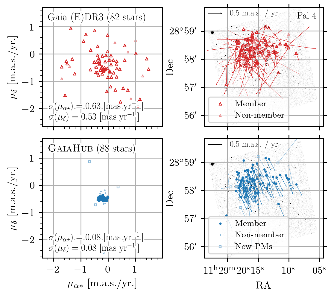
Figure 3: Comparison between the results obtained using Gaia and GaiaHub for Palomar 4 ($d_{\odot}=108.7\>{\rm kpc}$, $\Delta T=11.2$ years). The VPDs are shown in the left column and the PMs projected on the sky in the right column. Results from Gaia are represented in the top row by red symbols, new results from GaiaHub are shown by blue symbols in the bottom row. New PMs, not present in the Gaia EDR3 catalog are shown by open blue squares. Member stars, automatically selected by GaiaHub based on position in the VPD, are represented by large, darker markers. The larger dispersion observed in the Gaia VPD and PMs is a consequence of its larger uncertainties.

Here we present four examples of the quality of the results obtained with GaiaHub in comparison with those of Gaia EDR3 alone. In Figure 3 we show the impact that the precision of the PMs measurements has on the study of the internal kinematics of a stellar system by comparing Gaia’s VPD and the vectorial representation of its PMs in the observed field, with those obtained using GaiaHub in GC Palomar 4. Larger uncertainties in Gaia’s PMs are reflected in the perceived motion of the stars, and could lead to artificially large velocity dispersion measurements in stellar systems. Below, we show a more detailed comparison for three GCs ordered by their heliocentric distance.

NGC 6535

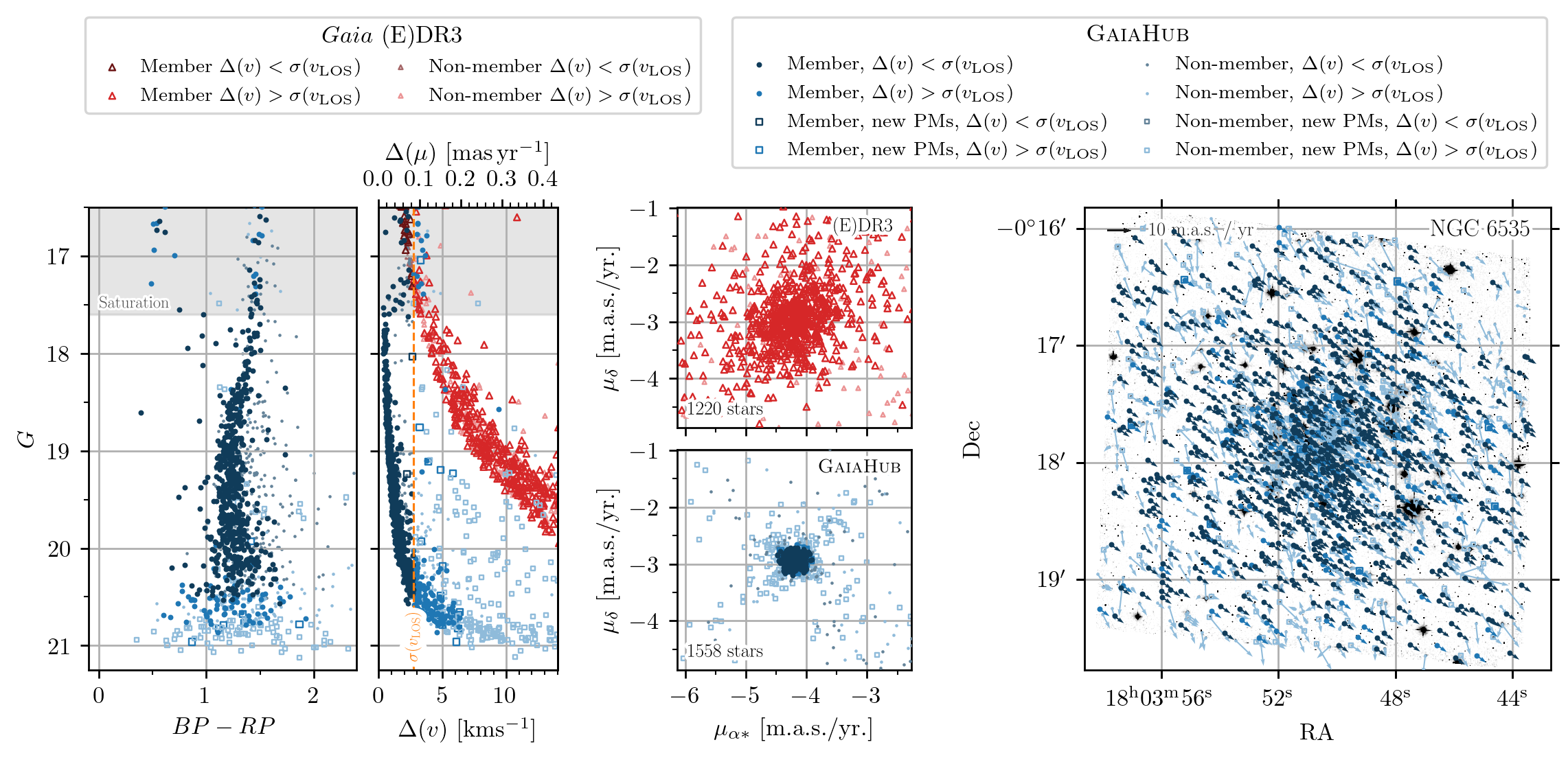
Figure 4: Summary of the results for NGC 6535 using GaiaHub and Gaia alone. From left to right the panels show the color-magnitude diagram (CMD), the PM uncertainties as a function of $G$ mag, the VPD for Gaia EDR3 (top) and GaiaHub (bottom), and the footprint of the analyzed area showing the PMs as vectors. Results from Gaia are represented in the second and third columns by open red triangles. New results from GaiaHub are shown by blue symbols. New PMs, not present in the Gaia EDR3 catalog are shown by open blue squares. Member stars, automatically selected by GaiaHub based on position in the VPD, are represented by large, darker markers. Stars whose PM uncertainty is below the central $\sigma(v_{\mathrm{LOS}})$ value of NGC 6535, marked by an orange vertical dashed line in the second panel ($2.4\pm 0.5\ {\rm{km\ s^{-1}}}\>$, see Table 1), are shown in dark blue. Non member stars are represented by light red (Gaia) and light blue (GaiaHub). The gray shaded area in two leftmost panels indicates the region of saturation for the deepest HST images. In the VPD (third column of panels), the dark red open triangles from the top panel (Gaia) compare to the dark blue dots from the bottom panel (GaiaHub). Notice that newly measured PMs that are not in the Gaia catalog (light-blue open squares) are not present in the Gaia’s VPD. The cross-like distribution observed in the VPD for very faint stars is likely caused by Gaia’s positional errors due to the observatory’s scanning law (see for example Bianchini et al., 2018). For clarity, the rightmost panel shows only measurements using GaiaHub.

Located at $d_{\odot}=6.8\>{\rm kpc}$, NGC 6535 provides a good example of the improvements in the PMs of faint stars in relatively nearby systems. The first HST epoch was taken in late March 2006, providing a total time baseline of 11.2 years. A comparison between the results from Gaia and GaiaHub is shown in Figure 4. GaiaHub clearly outperforms Gaia for magnitudes $G\gtrsim 17.25$, which in NGC 6535 includes almost all the observed stars below the horizontal branch (HB). The uncertainties are much smaller than those of Gaia alone, keeping values under the central line-of-sight velocity dispersion, $\sigma(v_{\mathrm{LOS}})=2.4\pm 0.4\ {\rm{km\ s^{-1}}}\>$, up to $G\sim 20.5$, well below the main sequence turn-off (MSTo). For comparison, the mean PM uncertainty for Gaia at $G\sim 20.5$ is $\sim 40\ {\rm{km\ s^{-1}}}\>$. The improved precision can be appreciated in the VPD, with GaiaHub’s PMs being much more concentrated. GaiaHub also derived PMs for 338 stars that have no PMs in the Gaia catalog. Despite having on average larger uncertainties than the rest of the GaiaHub’s measurements ($5\ {\rm{km\ s^{-1}}}\>\lesssim\Delta(v)\lesssim 15\ {\rm{km\ s^{-1}}}\>$) these newly measured PMs still have smaller uncertainties than most Gaia stars fainter than $G\sim 19.5$.

NGC 5053

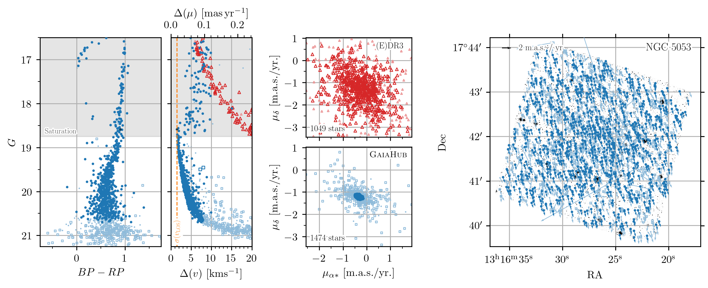
Figure 5: Summary of the results for NGC 5053 GC. Markers and colors coincide with those of Figure 4.

In Figure 5, we show a summary of the results obtained for NGC 5053. This is a relatively metal-poor cluster ($[Fe/H]=-2.27$) with very low velocity dispersion, $\sigma(v_{\mathrm{LOS}})=1.4\pm 0.2$. Because of this and the relatively large distance to the cluster, only one star has PMs uncertainties below the $\sigma(v_{\mathrm{LOS}})$ value. However, GaiaHub provides results far better than those of Gaia alone and allow to derive new PMs for 425 stars.

Pal 2

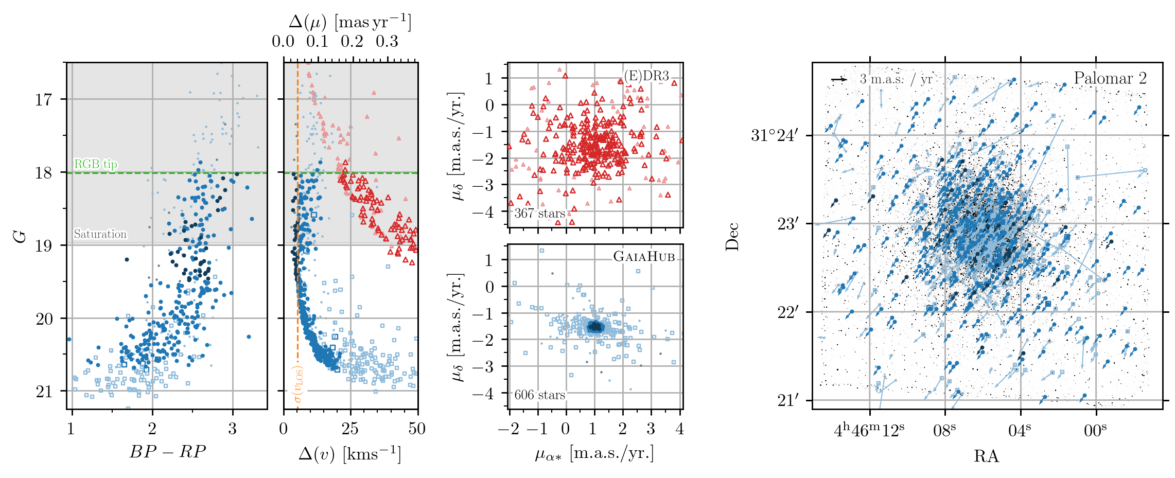
Figure 6: Summary of the results for Pal 2 GC. Markers and colors coincide with those of Figure 4. The RGB tip magnitude is shown by a green dashed horizontal line in the two leftmost panels. The central value of the central $\sigma(v_{\mathrm{LOS}})=5.1\ {\rm{km\ s^{-1}}}\>$ is taken from Baumgardt & Hilker (2018) (3rd version of the catalog, May 2021).

Pal 2 is located at 27.2 kpc from the Sun, which makes it a good target for GaiaHub. Figure 6 summarizes the results for GaiaHub. Despite the relatively large distance, GaiaHub allows us to derive PMs with uncertainties below $\sigma(v_{\mathrm{LOS}})$ values for many of its stars, as well as to derive new PMs for 239 stars.

NGC 2419

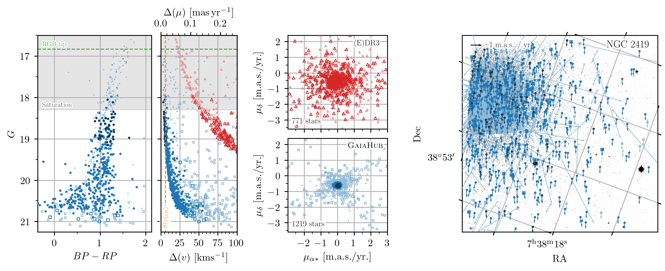
Figure 7: Summary of the results for NGC 2419. Markers and colors coincide with those of Figure 4.

The results for NGC 2419 are shown in Figure 7. Despite the large distance to NGC 2419, $d_{\odot}=82.6\>{\rm kpc}$, GaiaHub reaches accuracies at the level of its line-of-sight velocity dispersion, $\sigma(v_{\mathrm{LOS}})=4.0\pm 0.6\ {\rm{km\ s^{-1}}}\>$, for some of its stars, while showing average accuracies of $\sim 11\ {\rm{km\ s^{-1}}}\>$ at $G=20$. At the same magnitude, Gaia alone shows uncertainties of $\Delta(v)\sim 180\ {\rm{km\ s^{-1}}}\>$. The smallest uncertainty reached by Gaia EDR3, $\Delta(v)\sim 20\ {\rm{km\ s^{-1}}}\>$, is for the brightest stars at the tip of the red giant branch (TRGB) at $G\sim 16.75$. Future Gaia data releases will allow GaiaHub to measure hundreds of NGC 2419 stars below $\sigma(v_{\mathrm{LOS}})$ levels.

3.1.2 Dispersion, Anisotropy, and Ellipticity

For the 37 clusters in our final list, we used the PMs derived with GaiaHub to calculate the mean internal velocity dispersion along the radial, $\sigma(\mu_{\mathrm{R}})$, and tangential, $\sigma(\mu_{\mathrm{T}})$, directions with respect to the cluster’s center. To do so we use a maximum likelihood approach (as described in Section 3.1 of Watkins et al., 2015) that properly accounts for inflation of the observed PM dispersions by observational error. We then computed the velocity dispersion values in each direction as $\sigma(v)=4.7404\times d_{\odot}\times\sigma(\mu)$ and the sky-projected anisotropy, $\beta_{\rm sky}=1-\sigma(v_{\mathrm{T}})^{2}/\sigma(v_{\mathrm{R}})^{2}$. All sources of random errors were propagated following a Monte Carlo scheme in the case of the velocity dispersion, and analitically for the later computation of $\beta_{\rm sky}$, assuming a 10% error in the distance to the clusters. Our results are listed in Table 1.

Table 1: PM uncertainties and dispersions for GCs using GaiaHub and Gaia EDR3.

GC	$d_{\odot}$	$\Delta T$	$\Delta(v)_{\mathrm{Gaia}}$	$\Delta(v)_{\mathrm{\textsc{GaiaHub}}}$	$\sigma(\mu_{\mathrm{R}})$	$\sigma(\mu_{\mathrm{T}})$	$\sigma(v_{\mathrm{LOS}})$	$\sigma(v_{\mathrm{R}})$	$\sigma(v_{\mathrm{T}})$	$\beta_{\rm sky}$
	(kpc)	yr	$(\ {\rm{km\ s^{-1}}}\>)$	$(\ {\rm{km\ s^{-1}}}\>)$	$(\ {\rm{mas\ yr^{-1}}}\>)$	$(\ {\rm{mas\ yr^{-1}}}\>)$	$(\ {\rm{km\ s^{-1}}}\>)$	$(\ {\rm{km\ s^{-1}}}\>)$	$(\ {\rm{km\ s^{-1}}}\>)$
NGC6397	2.3	12.2	7.9	1.0	$0.352\pm 0.005$	$0.334\pm 0.005$	$4.50\pm 0.20$	$3.8\pm 0.4$	$3.6\pm 0.4$	$0.10\pm 0.04$
NGC6656	3.2	12.8	17.8	7.7	$0.408\pm 0.008$	$0.436\pm 0.009$	$7.80\pm 0.30$	$6.2\pm 0.6$	$6.6\pm 0.7$	$-0.14\pm 0.06$
NGC6752	4.0	11.6	12.9	1.2	$0.256\pm 0.005$	$0.227\pm 0.005$	$4.9\pm 0.4$	$4.9\pm 0.5$	$4.3\pm 0.4$	$0.21\pm 0.05$
NGC5139	5.2	11.4	15.2	6.5	$0.370\pm 0.012$	$0.329\pm 0.011$	$16.80\pm 0.30$	$9.1\pm 1.0$	$8.1\pm 0.9$	$0.21\pm 0.07$
NGC6535	6.8	11.2	21.2	1.9	$0.0530\pm 0.0024$	$0.0562\pm 0.0025$	$2.4\pm 0.5$	$1.71\pm 0.19$	$1.81\pm 0.20$	$-0.13\pm 0.14$
Terzan5	6.9	13.7	27.9	3.8	$0.385\pm 0.008$	$0.393\pm 0.008$		$12.6\pm 1.3$	$12.8\pm 1.3$	$-0.04\pm 0.06$
NGC6558	7.4	13.7	43.4	16.7	$0.076\pm 0.006$	$0.095\pm 0.007$	$3.1\pm 0.9$	$2.68\pm 0.35$	$3.3\pm 0.4$	$-0.53\pm 0.34$
NGC6325	7.8	7.1	42.6	8.4	$0.105\pm 0.008$	$0.109\pm 0.008$	$5.9\pm 1.3$	$3.9\pm 0.5$	$4.0\pm 0.5$	$-0.10\pm 0.23$
NGC6333	7.9	11.0	43.0	10.5	$0.1660\pm 0.0033$	$0.1661\pm 0.0034$		$6.2\pm 0.6$	$6.2\pm 0.6$	$-0.00\pm 0.06$
Lynga7	8.0	11.1	34.7	2.6	$0.0700\pm 0.0025$	$0.0715\pm 0.0025$		$2.66\pm 0.28$	$2.71\pm 0.29$	$-0.04\pm 0.10$
E3	8.1	11.1	18.5	1.7	$0.0019\pm 0.0021$	$0.0020\pm 0.0021$		$0.07\pm 0.08$	$0.08\pm 0.08$	$-0.0\pm 3.1$
NGC6642	8.1	13.2	39.4	9.0	$0.070\pm 0.006$	$0.063\pm 0.006$		$2.7\pm 0.4$	$2.41\pm 0.35$	$0.20\pm 0.22$
NGC6342	8.5	7.8	40.1	6.8	$0.085\pm 0.005$	$0.082\pm 0.005$	$5.2\pm 2.1$	$3.4\pm 0.4$	$3.3\pm 0.4$	$0.06\pm 0.16$
NGC6355	9.2	7.8	53.9	12.4	$0.127\pm 0.007$	$0.125\pm 0.007$		$5.5\pm 0.6$	$5.4\pm 0.6$	$0.03\pm 0.16$
NGC2808	9.6	10.8	36.5	4.0	$0.1465\pm 0.0029$	$0.1390\pm 0.0027$	$13.4\pm 1.2$	$6.7\pm 0.7$	$6.3\pm 0.6$	$0.10\pm 0.05$
NGC6139	10.1	7.3	60.3	14.1	$0.186\pm 0.006$	$0.198\pm 0.006$		$8.9\pm 0.9$	$9.5\pm 1.0$	$-0.14\pm 0.10$
NGC6256	10.3	7.8	52.7	7.1	$0.153\pm 0.007$	$0.157\pm 0.007$	$6.6\pm 2.6$	$7.5\pm 0.8$	$7.7\pm 0.8$	$-0.05\pm 0.13$
NGC6517	10.6	7.1	50.5	10.6	$0.172\pm 0.006$	$0.162\pm 0.006$		$8.6\pm 0.9$	$8.1\pm 0.9$	$0.11\pm 0.10$
NGC5946	10.6	7.8	49.8	10.4	$0.120\pm 0.005$	$0.121\pm 0.005$	$4.0\pm 2.9$	$6.0\pm 0.7$	$6.1\pm 0.7$	$-0.01\pm 0.12$
NGC6380	10.9	7.2	49.6	13.2	$0.183\pm 0.006$	$0.177\pm 0.006$		$9.4\pm 1.0$	$9.2\pm 1.0$	$0.06\pm 0.09$
Pal1	11.1	11.2	26.9	2.1	$0.005\pm 0.004$	$0.005\pm 0.004$		$0.26\pm 0.20$	$0.25\pm 0.19$	$0.0\pm 2.1$
NGC6453	11.6	7.1	64.6	69.7	$0.150\pm 0.007$	$0.175\pm 0.008$		$8.3\pm 0.9$	$9.6\pm 1.1$	$-0.36\pm 0.19$
Djorg1	13.7	13.3	63.8	5.7	$0.103\pm 0.008$	$0.101\pm 0.008$		$6.7\pm 0.8$	$6.6\pm 0.8$	$0.03\pm 0.21$
NGC5466	16.0	11.1	46.8	3.5	$0.0252\pm 0.0016$	$0.0245\pm 0.0016$	$1.70\pm 0.20$	$1.91\pm 0.23$	$1.86\pm 0.22$	$0.05\pm 0.18$
NGC5053	17.4	11.2	60.6	4.2	$0.0175\pm 0.0034$	$0.009\pm 0.004$	$1.40\pm 0.20$	$1.45\pm 0.31$	$0.8\pm 0.4$	$0.72\pm 0.28$
NGC5024	17.9	11.2	87.2	7.9	$0.0775\pm 0.0025$	$0.0739\pm 0.0026$	$4.4\pm 0.9$	$6.6\pm 1.0$	$6.3\pm 1.0$	$0.09\pm 0.06$
NGC6864	20.9	7.1	100.3	62.2	$0.085\pm 0.005$	$0.084\pm 0.005$	$10.3\pm 1.5$	$8.4\pm 1.0$	$8.3\pm 1.0$	$0.02\pm 0.16$
Pal13	26.0	6.9	70.9	10.6	$0.015\pm 0.009$	$0.015\pm 0.010$	$0.90\pm 0.30$	$1.8\pm 1.2$	$1.9\pm 1.2$	$-0.1\pm 2.0$
Terzan8	26.3	11.0	89.0	6.8	$0.011\pm 0.005$	$0.015\pm 0.005$		$1.3\pm 0.6$	$1.8\pm 0.7$	$-0.8\pm 2.1$
NGC6715	26.5	11.0	120.3	15.2	$0.0816\pm 0.0020$	$0.0839\pm 0.0021$	$10.50\pm 0.30$	$10.3\pm 1.1$	$10.5\pm 1.1$	$-0.06\pm 0.07$
Pal2	27.2	10.8	113.0	8.6	$0.030\pm 0.005$	$0.029\pm 0.005$		$3.9\pm 0.7$	$3.7\pm 0.7$	$0.1\pm 0.4$
Arp2	28.6	11.1	90.1	8.1	$0.013\pm 0.006$	$0.0025\pm 0.0023$		$1.7\pm 0.8$	$0.33\pm 0.31$	$0.96\pm 0.08$
NGC7006	41.2	7.6	123.9	19.2	$0.048\pm 0.006$	$0.024\pm 0.009$		$9.4\pm 1.5$	$4.7\pm 1.8$	$0.74\pm 0.19$
Pal15	45.1	7.6	147.1	15.3	$0.007\pm 0.006$	$0.006\pm 0.006$		$1.5\pm 1.2$	$1.4\pm 1.2$	$0.2\pm 1.9$
NGC2419	82.6	14.7	217.9	17.4	$0.010\pm 0.008$	$0.015\pm 0.009$	$4.0\pm 0.6$	$3.9\pm 3.2$	$6\pm 4$	$-1.4\pm 3.2$
Pal4	108.7	11.2	291.4	29.9	$0.011\pm 0.006$	$0.006\pm 0.004$		$5.5\pm 3.0$	$3.2\pm 2.3$	$0.6\pm 0.6$

Note. — Columns (2) and (8) are taken from Harris (1996) (2010 version). Columns (4) and (5) are the median error in the velocity measured from PMs at $G=20$ with Gaia EDR3 and GaiaHub, respectively. Columns (9) and (10) assume a 10% error in the distance to the cluster (2). Column (11) is the sky-projected anisotropy.

To assess the quality of the results, we compared the velocity dispersion along the three components in those clusters with available line-of-sight velocity dispersion, $\sigma(v_{\mathrm{LOS}})$, in the Harris (1996) catalog. This is shown in Figure 8. The dispersion along the three components is consistent, in general, except for NGC 2808, NGC 5139, and NGC 5024. Because $\sigma(v_{\mathrm{R}})$ and $\sigma(v_{\mathrm{T}})$ are mean values for all member stars within the HST field, in general we expect the central values of $\sigma(v_{\mathrm{LOS}})$ to be slightly larger. This is especially the case in clusters where the observed HST field is located at a large radial distance from the center of the cluster, such NGC 2808 and NGC 5139 (Omega Centauri). In fact, also relatively low dispersion values have been reported in the same field in $\omega$ Centauri using HST-only PMs (Bellini et al., 2018). That work separated the sample into multiple stellar populations, with the dominant one (MS-I) showing $\sigma(v_{\mathrm{R}})=8.46\pm 0.19\ {\rm{km\ s^{-1}}}\>$ and $\sigma(v_{\mathrm{T}})=8.16\pm 0.18\ {\rm{km\ s^{-1}}}\>$, both in very good agreement with the ones found using GaiaHub, i.e. $\sigma(v_{\mathrm{R}})=9.1\pm 1.0\ {\rm{km\ s^{-1}}}\>$ and $\sigma(v_{\mathrm{T}})=8.1\pm 0.9\ {\rm{km\ s^{-1}}}\>$.

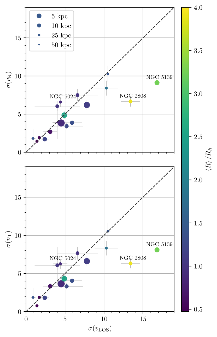
Figure 8: Mean internal velocity dispersion along the radial, $\sigma(v_{\mathrm{R}})$, and tangential, $\sigma(v_{\mathrm{T}})$, directions with respect to the center, for the GC sample described in the text and listed in Table 1. The color shade indicates the average distance of the analyzed data with respect to the center coordinates of the cluster. The size is inversely proportional to the Galactocentric distance to the cluster. The central velocity dispersion along the line-of-sight, $\sigma(v_{\mathrm{LOS}})$, was taken from Harris (1996) (2010 edition). The red dashed line shows a one-to-one relation. The data analyzed in NGC 2808 and NGC 5139 (Omega Cent) is located at 3.9 and 3.25 times their half-light radius, $R_{h}$, and therefore their $\sigma(v_{\mathrm{R}})$ and $\sigma(v_{\mathrm{T}})$ are expected to be smaller than $\sigma(v_{\mathrm{LOS}})$. NGC 5024 shows values not compatible with $\sigma(v_{\mathrm{LOS}})$ by $\sim 2.5\sigma$, probably caused by systematic errors not included in its error bars.

It is worth noticing that the uncertainties listed in Table 1 do not include possible systematic errors. We expect their impact to be small in nearby clusters, but they could be non-negligible for distant clusters. A possible example is NGC 5024, which shows an unusually large $\sigma(v_{\mathrm{R}})$ and $\sigma(v_{\mathrm{T}})$; more than $\sim 2.5\sigma$ larger than $\sigma(v_{\mathrm{LOS}})$. Lower values in $\sigma(v_{\mathrm{R}})$ and $\sigma(v_{\mathrm{T}})$ can be obtained with a more restrictive membership selection. For example, clipping the selection at $2\sigma$ instead of the $2.5\sigma$ used for the rest of the clusters produces $\sigma(v_{\mathrm{R}})$ and $\sigma(v_{\mathrm{T}})$ values that are consistent with $\sigma(v_{\mathrm{LOS}})$. In any case, it seems clear that NGC 5024 suffers from non-negligible systematic errors compared to its random uncertainties, and that this could also be the case for some other distant clusters. Moreover, because this is a demonstration paper for GaiaHub, we do not perform a thorough membership selection or error clipping prior to the $\sigma(\mu_{\mathrm{R}})$ and $\sigma(\mu_{\mathrm{T}})$ calculation, but use instead the automatic selection performed by GaiaHub. Hence, the results listed in Table 1 should be taken with caution, especially for those clusters located at small Galactic latitudes, where GaiaHub could be erroneously including some MW bulge stars as members. A more detailed analysis of the possible systematic errors that could be affecting GaiaHub’s results can be found in Section 4.

Indeed, the ratio between the sky-projected components of the velocity dispersion, $\sigma(v_{\mathrm{R}})$ and $\sigma(v_{\mathrm{T}})$, and the line-of-sight component, $\sigma(v_{\mathrm{LOS}})$, varies in direction and magnitude from one cluster to another. As commented above, systematic and observational effects could be behind these differences. However, the anisotropy could also be real, and be produced by the internal kinematics of the cluster. If this was the case, some correlation between the shape of the cluster and the ratio between the three components of the velocity dispersion could be present in our results. To check for this possibility, we compared the sky-projected ellipticity of the clusters ($\epsilon$) with the ratio between the average 1D dispersion observed in the plane of the sky with GaiaHub and the spectroscopic line-of-sight dispersion, $\sigma(v_{\rm sky})/\sigma(v_{\mathrm{LOS}})$, where $\sigma(v_{\rm sky})=\sqrt{\sigma(v_{\mathrm{R}})^{2}/2+\sigma(v_{\mathrm{T}})^{2}/2}$. Our results are shown in Figure 9, where we fit a straight line only to clusters whose HST observations are centered on the cluster or located not far away from it ($>1.5R_{h}$, 10 clusters). As expected, we observe a mild correlation (Spearman’s correlation: -0.74) between $\epsilon$ and $\sigma(v_{\rm sky})/\sigma(v_{\mathrm{LOS}})$, with round clusters ($\epsilon\lesssim 0.1$) being, in general, more isotropic than flattened ones. Also interesting is the fact that the intercept is close to (0, 1) which indicates that perfectly round clusters should be almost perfectly isotropic. A similar behavior was found by Watkins et al. (2015) by comparing the anistropy along the projected major and minor axes. These results would suggest that the internal kinematics of these clusters is indeed shaping them and causing, at least partially, some of the differences observed between $\sigma(v_{\mathrm{R}})$, $\sigma(v_{\mathrm{T}})$, and $\sigma(v_{\mathrm{LOS}})$.

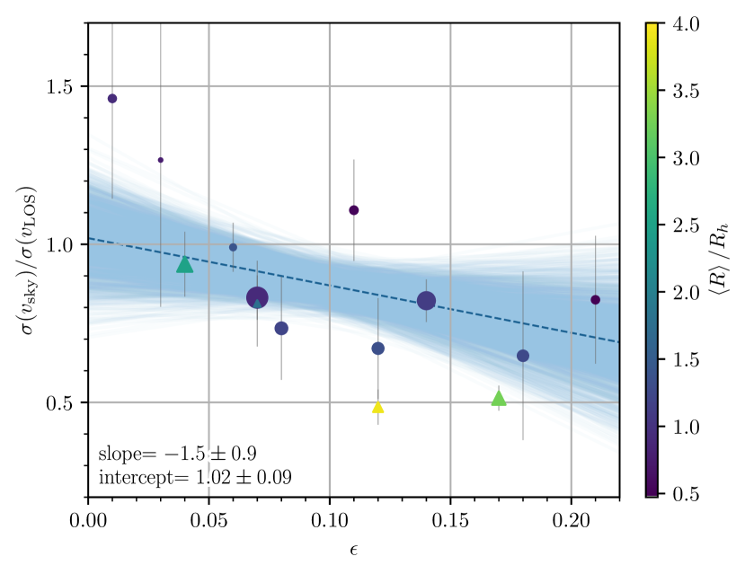
Figure 9: Ratio between the sky-projected velocity dispersion, $\sigma(v_{\rm sky})$ and the line-of-sight velocity dispersion, $\sigma(v_{\mathrm{LOS}})$, as a function of the sky-projected ellipticity $\epsilon$. Only clusters with uncertainties in $\sigma(v_{\rm sky})/\sigma(v_{\mathrm{LOS}})$ below 0.5 are shown. $\sigma(v_{\rm sky})$ is measured over the entire HST field, while $\sigma(v_{\mathrm{LOS}})$ correspond to the spectroscopic central velocity dispersion (Harris, 1996, 2010 version). Clusters whose observed HST field is located at distances larger than 1.5 times their $R_{h}$ are shown by triangles. The rest are shown by circles. The blue-dashed line shows the result from a straight-line fit to the clusters with $\left<R\right>/R_{h}<1.5$ (circles), and highlight a mild correlation (Spearman’s correlation: -0.74). The uncertainty of such fit is represented by the blue-shaded region. The rest of the markers coincide with those from Figure 8.

The distribution of anisotropy $\beta_{\rm sky}=1-\sigma(v_{\mathrm{T}})^{2}/\sigma(v_{\mathrm{R}})^{2}$ for all 37 clusters is shown in Figure 10. The distribution is slightly tilted towards radially anisotropic values, with a median value of $\tilde{\beta_{\rm sky}}=0.026$ and an error-weighted mean value of $\overline{\beta_{\rm sky}}=0.057\pm 0.016$. Most of our clusters fit completely in our HST images or have been observed at distances reaching or exceeding their half-light radii ($R_{h}$). Thus our results are consistent with findings of Watkins et al. (2015) that globular clusters generally become mildly radially anisotropic towards $R_{h}$. Similar results were also found by Vasiliev & Baumgardt (2021), with half of the clusters in their sample showing radial anisotropy and the rest being either tangentially anisotropic or isotropic.

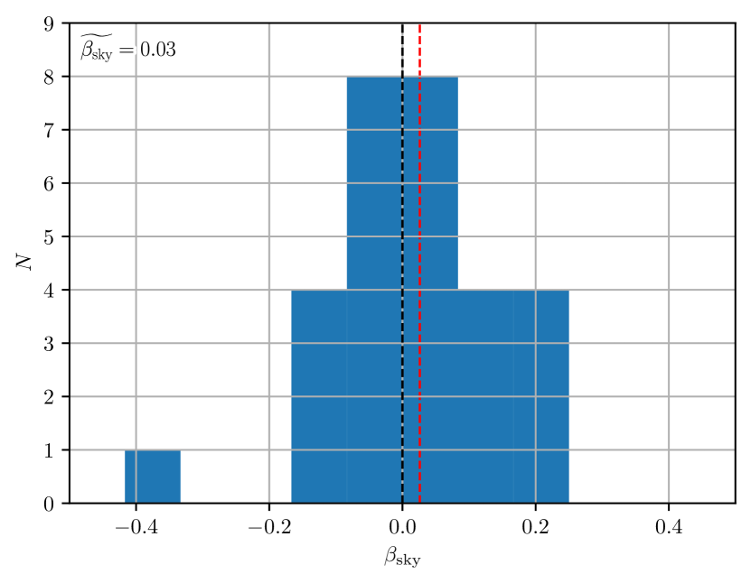
Figure 10: Distribution of the anisotropy, $\beta_{\rm sky}=1-\sigma(v_{\mathrm{T}})^{2}/\sigma(v_{\mathrm{R}})^{2}$, of the 37 clusters listed in Table 1. A vertical red dashed line shows the median value of the distribution $\tilde{\beta_{\rm sky}}=0.026$.

3.2 Dwarf Spheroidal Galaxies

Table 2: PM uncertainties and dispersions for dSphs using GaiaHub and Gaia EDR3.

Name	$d_{\odot}$	$\Delta T$	$\Delta(v)_{\mathrm{Gaia}}$	$\Delta(v)_{\mathrm{\textsc{GaiaHub}}}$	$\sigma(\mu_{\mathrm{R}})$	$\sigma(\mu_{\mathrm{T}})$	$\sigma(v_{\mathrm{LOS}})$	$\sigma(v_{\mathrm{R}})$	$\sigma(v_{\mathrm{T}})$	$\beta_{\rm sky}$
	(kpc)	yr	$(\ {\rm{km\ s^{-1}}}\>)$	$(\ {\rm{km\ s^{-1}}}\>)$	$(\ {\rm{mas\ yr^{-1}}}\>)$	$(\ {\rm{mas\ yr^{-1}}}\>)$	$(\ {\rm{km\ s^{-1}}}\>)$	$(\ {\rm{km\ s^{-1}}}\>)$	$(\ {\rm{km\ s^{-1}}}\>)$
Draco	$76\pm 6$	12.6	167.0	11.9	$0.025\pm 0.006$	$0.016\pm 0.007$	$9.1\pm 1.2(9.1\pm 1.2)$	$9.0\pm 2.3$	$5.8\pm 2.6$	$0.59\pm 0.42$
Sculptor	$86\pm 6$	14.7	136.1	8.9	$0.0202\pm 0.0033$	$0.018\pm 0.004$	$9.2\pm 1.4(8.8\pm 1.8)$	$8.2\pm 1.4$	$7.1\pm 1.7$	$0.25\pm 0.43$
Sextans	$86\pm 4$	12.9	409.0	35.2	$0.08\pm 0.05$	$0.072\pm 0.032$	$7.9\pm 1.3(6.8\pm 2.4)$	$32\pm 17$	$29\pm 13$	$0.16\pm 1.32$
Fornax	$147\pm 12$	14.2	243.6	16.1	$0.012\pm 0.005$	$0.018\pm 0.006$	$11.7\pm 0.9(9.2\pm 1.8)$	$8.0\pm 3.5$	$13\pm 4$	$-1.54\pm 2.71$

Note. — Columns (2) and (8) are taken from McConnachie (2012). Values in parentheses in column (8) are measured within the area covered by this study using different data available from the literature (Walker et al., 2009, 2015). Columns (4) and (5) are the median error in the velocity measured from PMs at $G=20$ with Gaia EDR3 and GaiaHub, respectively. Column (11) shows the sky-projected anisotropy with two significant figures.

DSphs are frequently invoked as testbeds of the nature of dark matter (DM), particularly concerning the presence or absence of cusps as predicted by $\Lambda$CDM. Line-of-sight velocity surveys have suggested a generally low, nearly constant density in the cores of these galaxies (e.g. Battaglia et al., 2008; Walker & Peñarrubia, 2011; Amorisco & Evans, 2012; Brownsberger & Randall, 2021), which could point to either strong effects of baryonic feedback or alternative theories of DM. On the other hand, some authors found profiles that are fully consistent with $\Lambda$CDM expectations (Strigari et al., 2010), or at least compatible with both scenarios (Genina et al., 2018). Such variety of results is partly fueled by strong model degeneracies remaining in the mass profile due to the lack of accurate tangential velocity data (Strigari et al., 2018; Read et al., 2021).

GaiaHub can aid in this particular problem by providing tangential velocities for stars in some of the dSph satellites of the MW with accuracies below the internal velocity dispersion. Here, we run GaiaHub on four of the classical dSph galaxies, and provide a preliminary assessment of the quality of the results. In Table 2, we summarize some basic properties of the galaxies, and the derived random uncertainties for stars in the fields analyzed with GaiaHub at $G=20$. In three of the galaxies, Draco, Sculptor, and Fornax, GaiaHub manages to derive individual PMs with accuracies below the central $\sigma(v_{\mathrm{LOS}})$ of the galaxies. The velocity dispersions are estimated following the same maximum likelihood approach that we used for the GCs. Below we analyze the results in more detail.

3.2.1 Detailed results

Draco dSph

We derived PMs for stars in the Draco dSph, following the examples described in the Appendix A. Specifically, we used the automatic membership selection in order to use only member stars to make the epoch alignment and increased the membership selection clipping probability from $3\sigma$ to $5\sigma$. At the time of writing this paper, GaiaHub found 77 suitable HST images in Draco arranged across four fields. Three fields located close to the center of the galaxy and a more distant field with just one image and very few stars. We chose to use the images from the three central fields (GO-10229 & GO-10812).

Figure 11: Summary of the results for the Draco dSph galaxy. Markers and colors coincide with those of Figure 4. Results from Massari et al. (2020) are shown in the second panel for comparison by gold colored dots.

As described in Section 2.2 and Appendix B, after downloading all the images, GaiaHub runs a first iteration using all the stars available to establish a common reference frame and derive the PMs. Then, it uses the PMs to select co-moving stars, i.e. members of Draco, and repeats the process using only those to establish the reference frame. The process converged after 3 iterations, using 127 stars for the alignment between epochs and providing PMs for 151 stars. The results are summarized in Figure 11.

In the case of Draco, GaiaHub is able to derive individual PMs with uncertainties below $\sigma(v_{\mathrm{LOS}})=9.1\ {\rm{km\ s^{-1}}}\>$ for 21 stars. The number of member stars between the TRGB and $G=20$ is 64, with a median velocity error of $9.1\ {\rm{km\ s^{-1}}}\>$. The effect of having such a small uncertainties compared with Gaia alone can be observed in the concentration of the stars in the VPD, with member stars clustering much more tightly in the GaiaHub results. GaiaHub also manages to derive PMs for up to 18 stars without previous EDR3 PMs, 6 of them with uncertainties below $100\ {\rm{km\ s^{-1}}}\>$.

Draco appears to be radially anisotropic, with $\beta_{\rm sky}=0.6\pm 0.4$, $\sigma(v_{\mathrm{R}})=9.0\pm 2.3\ {\rm{km\ s^{-1}}}\>$ and $\sigma(v_{\mathrm{T}})=5.8\pm 2.7\ {\rm{km\ s^{-1}}}\>$. We computed the line-of-sight velocity dispersion within the area covered in this work using radial velocity measurements from Walker et al. (2015). The obtained value, $\sigma(v_{\mathrm{LOS}})^{\prime}=9.1\pm 1.2\ {\rm{km\ s^{-1}}}\>$, is based on 39 common stars, and coincides with values found in the literature for the central $\sigma(v_{\mathrm{LOS}})$ of Draco (McConnachie, 2012). We used this value to estimate the intrinsic anisotropy $\beta=1-\sigma(v_{\mathrm{T}})^{2}/[\sigma(v_{\mathrm{LOS}})^{2}+\sigma(v_{\mathrm{R}})^{2}-\sigma(v_{\mathrm{T}})^{2}]$ (Equation 1 in Massari et al., 2017) at the distance of the observed fields. Our results, $\beta=0.75\pm 0.30$, are compatible with those from Massari et al. (2020) who found $\sigma(v_{\mathrm{R}})=11.0_{-1.5}^{+2.1}\ {\rm{km\ s^{-1}}}\>$, $\sigma(v_{\mathrm{T}})=9.9_{-3.1}^{+2.3}\ {\rm{km\ s^{-1}}}\>$ and a 3D radial anisotropy of $\beta=0.25_{-1.38}^{+0.47}$.

Sculptor dSph

As with Draco, we used the automatic membership selection and increased the membership selection clipping probability from $3\sigma$ to $5\sigma$. At the time of writing this paper, GaiaHub found 11 suitable HST images in Sculptor arranged in two fields (from HST program GO-9480). We chose to use all of the images.

In the particular case of Sculptor, the process of selecting group members did not converge but started to oscillate between two possible solutions after 3 iterations. We decided to stop the execution after 4 iterations, which produces the solution for which more stars labeled as members and uses 173 stars for the alignment between epochs. GaiaHub produced PMs for 225 stars, $\sim 14$% more than Gaia alone (197 stars). The results are summarized in Figure 12.

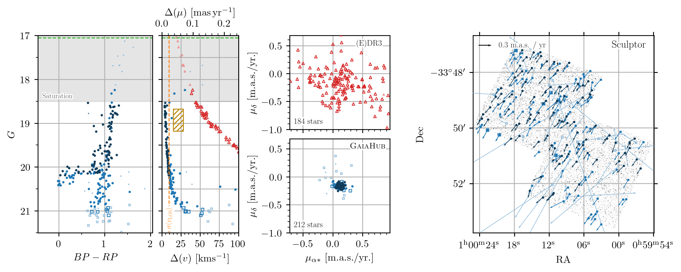
Figure 12: Summary of the results for the Sculptor dSph galaxy. Markers and colors coincide with those of Figure 4. For comparison, we show the reported PM uncertainty range by Massari et al. (2018) as a gold colored hatched box in the second panel.

In the case of Sculptor, GaiaHub is able to derive individual PMs with uncertainties below the $\sigma(v_{\mathrm{LOS}})$ for 81 stars. The number of member stars between the TRGB and $G=20$ is 89, with a median velocity uncertainty of $6.8\ {\rm{km\ s^{-1}}}\>$. Up to 28 new PMs for stars without measurements in the EDR3 catalog were derived by GaiaHub, 13 of them with uncertainties below $100\ {\rm{km\ s^{-1}}}\>$.

Using GaiaHub’s PMs and assuming a distance of $d_{\odot}=85.9\pm 5.5$ (McConnachie, 2012), we find a velocity dispersion in the radial and tangential direction of $\sigma(v_{\mathrm{R}})=8.2\pm 1.4\ {\rm{km\ s^{-1}}}\>$ and $\sigma(v_{\mathrm{T}})=7.1\pm 1.7\ {\rm{km\ s^{-1}}}\>$, respectively (propagating the error in distance). These values, are in good agreement with those derived by Massari et al. (2018), where combining HST and Gaia DR1 data they found $\sigma(v_{\mathrm{R}})=11.5\pm 4.3\ {\rm{km\ s^{-1}}}\>$ and $\sigma(v_{\mathrm{T}})=8.5\pm 3.2\ {\rm{km\ s^{-1}}}\>$. This would indicate that Sculptor is radially anisotropic at the position of the observed HST fields, amid a large relative uncertainty in the measurement ($\beta=0.25\pm 0.43$). As with Draco, we use $v_{\mathrm{LOS}}$ measurements from Walker et al. (2009) to estimate $\sigma(v_{\mathrm{LOS}})^{\prime}=8.8\pm 1.8\ {\rm{km\ s^{-1}}}\>$ in the observed region (based on 15 stars). The value for the intrinsic anisotropy, $\beta=0.46\pm 0.44$, also indicates that Sculptor is mildly radially anisotropic.

Sextans dSph

Two suitable HST fields were found for Sextans. However, due to the scarce number of stars, and the low ratio between members and foreground MW’s stars, results for only one field converged and produced PMs (GO-10229, 15 images). Results are summarized in Figure 13. In total, 17 stars were measured in the field, with 15 of them being classified as members. For these stars, GaiaHub yielded far more precise results than those of Gaia alone, with uncertainties around $35\ {\rm{km\ s^{-1}}}\>$ at $G=20$ compared to uncertainties of $\sim 400\ {\rm{km\ s^{-1}}}\>$ for Gaia. However, the scarce number of measured PMs and their relatively large uncertainties compared to the central velocity dispersion of Sextans ($\sigma(v_{\mathrm{LOS}})=7.9\pm 1.3$), did not allow us to obtain statistically sound results for the dispersion velocity. The derived values, $\sigma(v_{\mathrm{R}})=32\pm 17$ and $\sigma(v_{\mathrm{T}})=29\pm 13$, are far too high compared with $\sigma(v_{\mathrm{LOS}})$. This could also indicate that non-negligible systematic effects are affecting our data, but with only 15 member stars, our tests remained inconclusive (see Section 4).

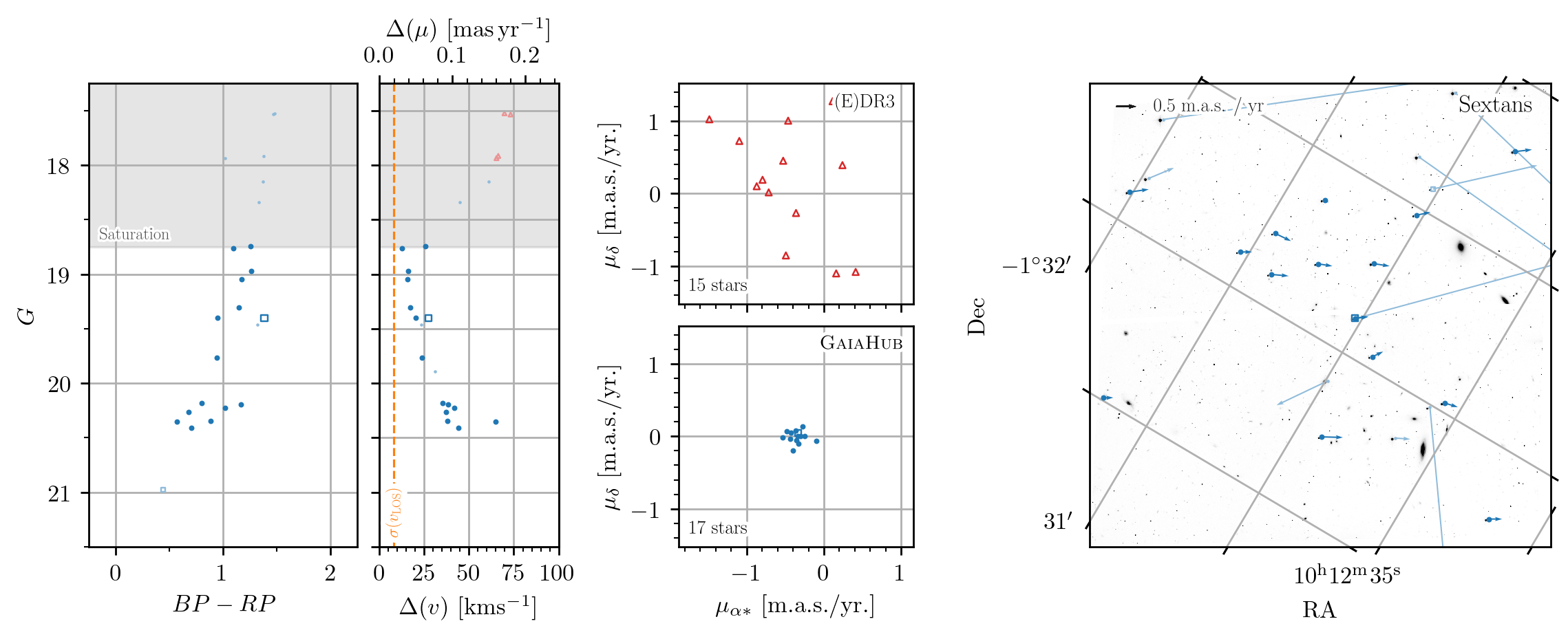
Figure 13: Summary of the results for the Sextans dSph galaxy. Markers and colors coincide with those of Figure 4.

Fornax dSph

GaiaHub found 6 suitable HST images in Fornax arranged in a single field (GO-9480 and GO-9575). We chose to use all of the images. GaiaHub converged after two iterations, using 54 stars for the alignment between epochs and providing PMs for 198 stars. The results are summarized in Figure 14.

Figure 14: Summary of the results for the Fornax dSph galaxy. Markers and colors coincide with those of Figure 4.

Despite its large heliocentric distance ($d_{\odot}=147\pm 12\>{\rm kpc}$), GaiaHub is able to derive individual PMs with uncertainties below the $\sigma(v_{\mathrm{LOS}})=11.7\pm 0.9\ {\rm{km\ s^{-1}}}\>$ for 21 stars in Fornax. The number of member stars between the TRGB and $G=20$ is 38, with a median velocity uncertainty of $11.6\ {\rm{km\ s^{-1}}}\>$ and a typical uncertainty at $G=20$ of $16.1\ {\rm{km\ s^{-1}}}\>$. GaiaHub also manages to derive PMs for up to 107 stars without previous EDR3 PMs, 39 of them with uncertainties below $100\ {\rm{km\ s^{-1}}}\>$. As with previous examples, the gain in precision with respect to Gaia EDR3 results is easily noticeable in the VPD, with member stars clustering much more tightly on the GaiaHub’s VPD.

The obtained velocity dispersion, $\sigma(v_{\mathrm{R}})=8.0\pm 3.5\ {\rm{km\ s^{-1}}}\>$ and $\sigma(v_{\mathrm{T}})=13\pm 4\ {\rm{km\ s^{-1}}}\>$ would suggest that Fornax is tangentially anisotropic at the location of the HST fields. However, the relatively large uncertainties of our measurements do not allow us to reach any strong conclusion ($\beta=-1.5\pm 2.7$). Measurements of the dispersion along the line-of-sight ($\sigma(v_{\mathrm{LOS}})^{\prime}=9.2\pm 1.8$, based on 16 stars) do not allow for any improvement in Fornax, with uncertainties that make our results also, compatible with both radially and tangentially anisotropic.

3.2.2 Anisotropy and caveats

GaiaHub provided far more precise results than those of Gaia alone in all the cases analyzed in this work. Our results show that the general tendency among the dSphs satellites of the MW is to be radially anisotropic, with the exception of Fornax. This is compatible with findings of Massari et al. (2018, 2020), who used the same instruments and similar methods but previous Gaia data releases, and hence shorter time baselines.

Despite the clear improvement, our results are still affected by relatively large uncertainties that prevent us from making any strong claim about the anisotropy of the dSphs, except for Draco and perhaps Sculptor. Nevertheless, it is interesting that Fornax is the only system that appears to be tangentially anisotropic (amid very large uncertainties). Fornax exhibits relatively complex rotation patterns both along the line-of-sight (del Pino et al., 2017) and on the plane of the sky (Martínez-García et al., 2021). It is also the only galaxy in our sample that host GCs and known stellar shells. This, among other conspicuous features of its star formation history, has led some authors to claim that Fornax could be the remnant of a merger (Amorisco & Evans, 2012; del Pino et al., 2015). If this was the case, the galaxy’s peculiar kinematics could be behind its possible tangential anisotropy. Future Gaia releases will increase both the positional accuracy and the time baseline, which will greatly improve the uncertainties and shed light on these questions.

4 Systematic errors

Both observatories, Gaia and HST, show undesired systematic errors that affect their astrometric measurements. In the case of Gaia, the magnitude and direction of these systematics are known to be dependent on the considered position in the sky, the apparent brightness of the stars and their color. While some characterization of these systematics exists, (for example Lindegren et al., 2021; Fardal et al., 2021; Vasiliev & Baumgardt, 2021), correcting for their effects has turned out to be difficult. Moreover, the behavior of systematics on angular scales as small as an HST field are effectively unconstrained. A solution some authors adopt is to offer alternative astrometric zero-points measured using stationary sources (distant quasars) located within a few degrees around the object of interest (van der Marel et al., 2019; del Pino et al., 2021; Martínez-García et al., 2021; Battaglia et al., 2021). For HST, the positional accuracies for stars are affected by several factors, most importantly the geometric distortions affecting the focal plane, CCD charge transfer inefficiency, and breathing of the telescope (i.e. the expansion or contraction of the observatory due to heating by solar radiation). These effects are all corrected by the HST data-processing pipeline and/or the data reduction performed by GaiaHub. However, the corrections are never perfect, and residual systematics may remain. The combination of the two observatories can therefore be affected by systematic errors that are difficult to characterize.

One way to estimate the systematics is to analyze the velocity dispersion $\sigma(\mu)$ derived from PMs, and compare it to other independent measurements. In general, $\sigma(\mu)$ is the convolution of the intrinsic PM dispersion of the system, $\sigma_{int}(\mu)$, the random uncertainties, $\Delta(\mu)$, and the systematics, $\Delta_{sys}(\mu)$. Therefore, systematic uncertainties could be derived as $\Delta_{sys}=\sqrt{\sigma(\mu)^{2}-\Delta(\mu)^{2}-\sigma_{int}(\mu)^{2}}$. While independent measurement of $\sigma_{int}(\mu)$ mostly do not exist at the moment, measurements of the central velocity dispersion along the line-of-sight, $\sigma(v_{\mathrm{LOS}})$ are fairly common. By assuming that the internal dispersion of the stellar object is approximately isotropic in all directions, we can substitute $\sigma_{int}(\mu)$ by $\sigma(v_{\mathrm{LOS}})$ in the relation above to infer systematic errors. The best objects to try this method are GCs, whose sphericity suggests that both quantities should indeed be similar.

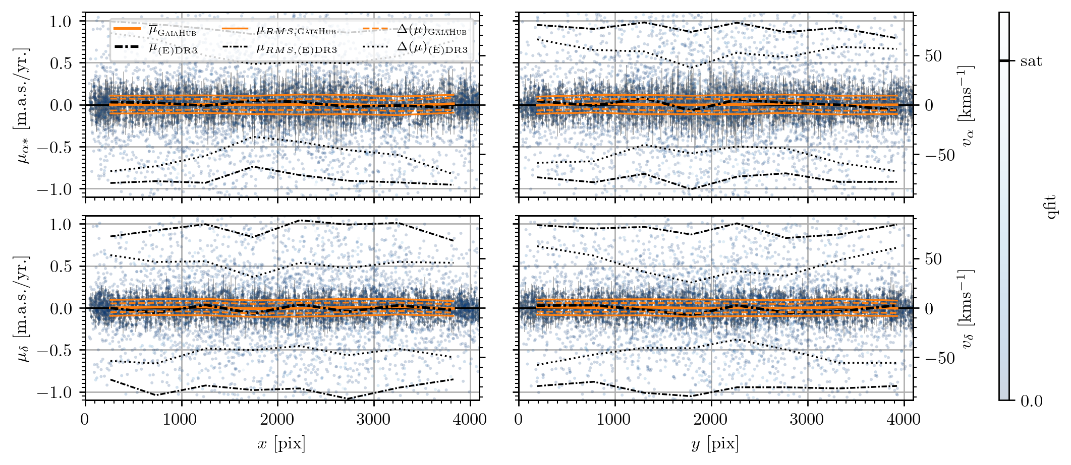
Figure 15: Relative stellar PMs (and velocities) in NGC 5024 as a function of the CCD’s position in the HST images. The mean value of $\mu_{\alpha\star}$ and $\mu_{\delta}$ ($\overline{\mu}$), the RMS ($\mu_{\rm RMS}$), and the mean random error ($\Delta(\mu)$) are shown by thick, thin, and thin-dashed orange lines, respectively, in the case of GaiaHub. For comparison, the same statistics are shown for Gaia by thick, thin, dotted-dashed and dotted lines in black color. All statistics are computed within 8 quantiles along both CCD coordinates $(x,y)$. The color scale indicates the mean value of goodness of the PSF fit of the star in the HST data (qfit). Stars with colors lighter than the qfit = "sat" are saturated in the HST images. Only member stars show error bars. The large difference between the RMS and the random uncertainties cannot be explained by the internal velocity dispersion of the cluster and may indicate the presence of systematic errors.

As a demonstration we analyze NGC 5024, a cluster that we suspect suffers from systematic errors due to the high stellar crowding observed in its central region. This may be behind the relatively large values of $\sigma(v_{\mathrm{R}})=6.6\pm 1\ {\rm{km\ s^{-1}}}\>$ and $\sigma(v_{\mathrm{T}})=6.3\ {\rm{km\ s^{-1}}}\>$, $\sim 2\sigma$ above the central velocity dispersion along the line-of-sight, $\sigma(v_{\mathrm{LOS}})=4.4\pm 0.9\ {\rm{km\ s^{-1}}}\>$. Figure 15 shows the relative PMs along the $x$ and $y$ axes of the HST CCD for NGC 5024. Results from GaiaHub are remarkably stable compared to those of Gaia alone, with the average relative PMs, $\overline{\mu}$ (orange line) forming a straight line centered at zero along both directions in the CCD. However, for this particular cluster, $\mu_{\rm RMS}$ (orange solid thin lines) is consistently larger than $\Delta(\mu)$ (orange dashed thin lines). This difference cannot be explained by its internal dispersion alone if we assume that NGC 5024 is isotropic. Applying the expression from the previous paragraph, we obtained values of $\Delta_{sys}(\mu_{\alpha\star})\sim 71\ \mu{\rm as}\,{\rm yr}^{-1}$ and $\Delta_{sys}(\mu_{\delta})\sim 56\ \mu{\rm as}\,{\rm yr}^{-1}$, equivalent to $\sim 6$, and $\sim 5\ {\rm{km\ s^{-1}}}\>$, respectively ($\sim 0.79$ and $\sim 0.62\ {\rm{mas}}\>$ if we multiply by $\Delta(T)=11.24$ years for NGC 5024). Indeed, if we add in quadrature these values to the PMs nominal uncertainties and repeat our calculations for the sky-projected dispersions, we obtain $\sigma(v_{\mathrm{R}})=4.7\pm 0.6\ {\rm{km\ s^{-1}}}\>$ and $\sigma(v_{\mathrm{T}})=4.5\pm 0.6\ {\rm{km\ s^{-1}}}\>$, values that are fully compatible with $\sigma(v_{\mathrm{LOS}})$. It is important to point out that, because this method assumes that the cluster is isotropic, i.e. $\sigma(v_{\mathrm{R}})\sim\sigma(v_{\mathrm{T}})\sim\sigma(v_{\mathrm{LOS}})$, the fact that adding these values to the final error budget results in compatible dispersion values along the three dimensions should not be interpreted as these being an accurate measurement of the systematics.

Repeating this calculation for all the GCs with $\sigma(\mu_{\alpha\star})$ or $\sigma(\mu_{\delta})$ greater than $\sigma(v_{\mathrm{LOS}})$ from our sample yields a median, all-sky $\widetilde{\Delta_{sys}}(\mu_{\alpha\star},\mu_{\delta})\sim(25,15)\ \mu{\rm as}\,{\rm yr}^{-1}$ ($\sim 0.27$ and $\sim 0.16\ {\rm{mas}}\>$ when multiplying by the temporal baseline). As commented above, in reality the clusters might well be non-isotropic (see Section 3.1.2), and therefore these values should serve only as an estimation of the typical maximum systematic errors currently affecting GaiaHub’s results.

Another way to assess the impact of systematics is to analyze the RMS scatter observed in the PMs ($\mu_{\rm RMS}$) and compare it to their random uncertainties, $\Delta(\mu)$. In clusters where the intrinsic velocity dispersion is low, $\mu_{\rm RMS}$ and $\Delta(\mu)$ should be similar unless the effects from systematics are not negligible. The cluster NGC 5053 seems to be an ideal example target; it shows a very low velocity dispersion, $\sigma(v_{\mathrm{LOS}})=1.4\pm 0.2$, has a large number of stars observed by Gaia, and is located at a large distance ($d_{\odot}=17.4\>{\rm kpc}$), where systematics should dominate the total uncertainty budget. Because of the relatively large distance to the cluster and its low line-of-sight velocity dispersion, only one star has PMs uncertainties below the $\sigma(v_{\mathrm{LOS}})$ value. However, the results are clearly better than those of Gaia alone (see Figure 5), and allow us to perform a detailed analysis of the distribution of the PMs and their random uncertainties as a function of different parameters.

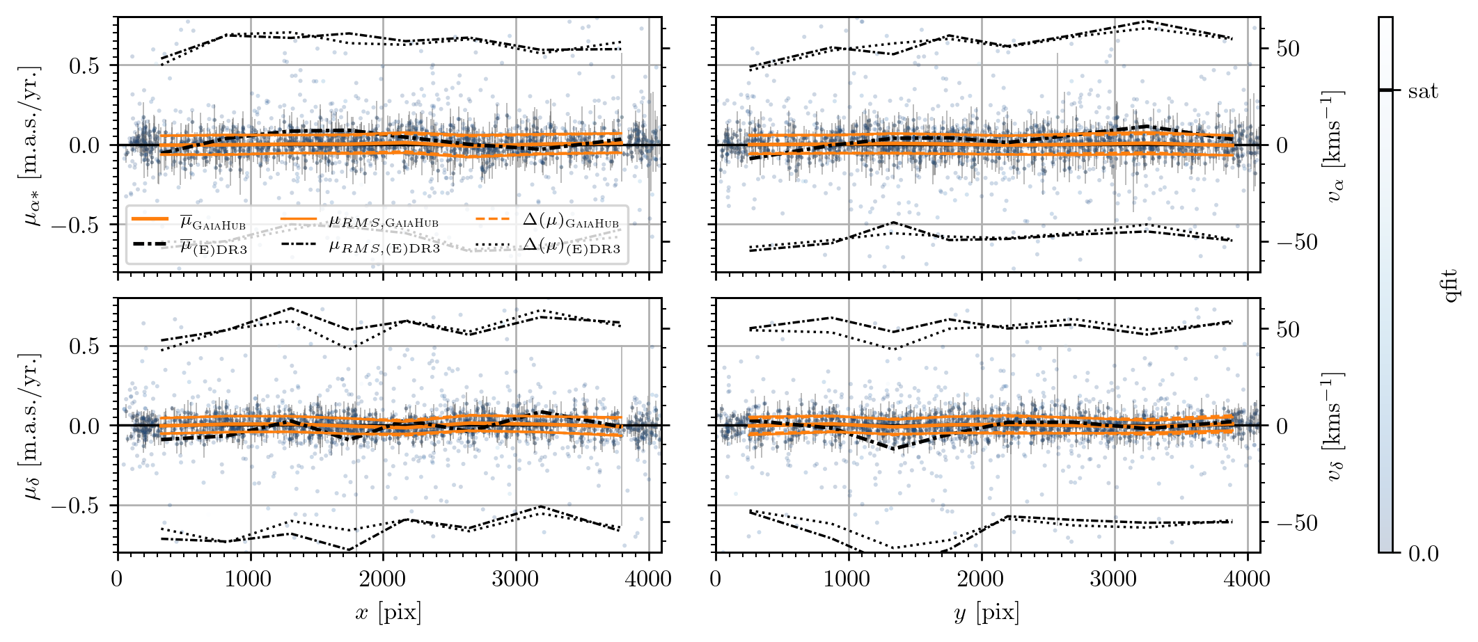
Figure 16: Relative stellar PMs in NGC 5053 as a function of the CCD’s position in the HST images. Markers and colors coincide with those of Figure 15. Notice that in this case, the RMS and the random uncertainties are almost identical, indicating that systematics do not have a large impact on the results.

Figure 16 shows the relative PMs along the $x$ and $y$ axes of the HST CCD for NGC 5053. As with NGC 5024, results obtained for NGC 5053 with GaiaHub are far more stable than those from Gaia alone. However, in this case $\mu_{\rm RMS}$ is very similar to $\Delta(\mu)$, which would indicate that systematics errors have a negligible effect on the derived PMs.

The same relative PMs are shown as a function of the stellar magnitudes, and color in Figures 17 and 18, respectively. In general, GaiaHub’s results outperforms those from Gaia in stability and precision, and show mean random uncertainties that are very close to the observed RMS. Assuming that $\sigma_{int}(\mu)\approx\sigma(v_{\mathrm{LOS}})$, we can calculate the systematics as $\Delta_{sys}(\mu)=\sqrt{\sigma(\mu)^{2}-\Delta(\mu)^{2}-\sigma(v_{\mathrm{LOS}})^{2}}$. In the case of NGC 5053, this yields systematic errors on the order of $\Delta_{sys}(\mu_{\alpha\star})\sim 13\ \mu{\rm as}\,{\rm yr}^{-1}$ and $\Delta_{sys}(\mu_{\delta})\sim 10\ \mu{\rm as}\,{\rm yr}^{-1}$ ($\sim 0.15$ and $\sim 0.11$ mas with $\Delta(T)=11.3$ years for NGC 5053).

Systematic errors are expected to have contributions from HST, Gaia, and from the epoch alignment procedure itself, which makes disentangling their origin far more complicated than trying to measure their impact on the final PMs. However, we noticed that the systems that seem to be more affected by systematics show larger differences between $\mu_{\rm RMS,{\rm(E)DR3}}$ and $\Delta(\mu)_{\rm(E)DR3}$, regardless of their internal dispersion. This can be seen, for example, by comparing both curves in Figures 15 and  16. In the case of NGC 5053, both curves are practically one on top of the other, while in NGC 5024 $\Delta(\mu)_{\rm(E)DR3}$ is $\sim 1.8$ times smaller than $\mu_{\rm RMS,{\rm(E)DR3}}$ and cannot account for the observed dispersion. This could indicate that the nominal errors in Gaia are largely underestimated in NGC 5024 and therefore that Gaia PMs are affected by larger systematics in this case. Moreover, the systematic error values found for NGC 5053 are similar to those reported for Gaia EDR3 PMs at small scales ($0-0.1\arcdeg$) for the entire sky (Lindegren et al., 2021; Martínez-García et al., 2021; Vasiliev & Baumgardt, 2021), which may indicate that, if present, most of the systematics errors found in GaiaHub’s results are being propagated from those affecting Gaia’s stellar positions. Therefore, GaiaHub would not be introducing any noticeable systematic errors in the final results, and thus we expect its results to greatly improve as Gaia’s systematics drop in future data releases.

However, we should point out that this might not be the case for other stellar systems. Systematics affecting both instruments vary depending on the quality of the used HST and Gaia data, which could result in very different scenarios depending on the considered object. Furthermore, running GaiaHub with different options also has on impact on the results, and thus could mitigate or increase the impact of systematic errors. Finally, it is also worth noticing that the estimations provided here may be not valid with future Gaia releases or increased time baselines. How to best characterize or try to correct for systematics will ultimately depends on the scientific goals of the project. Therefore, we recommend the user to exercise extreme caution and to thoroughly analyze the results before reaching any scientific conclusions.

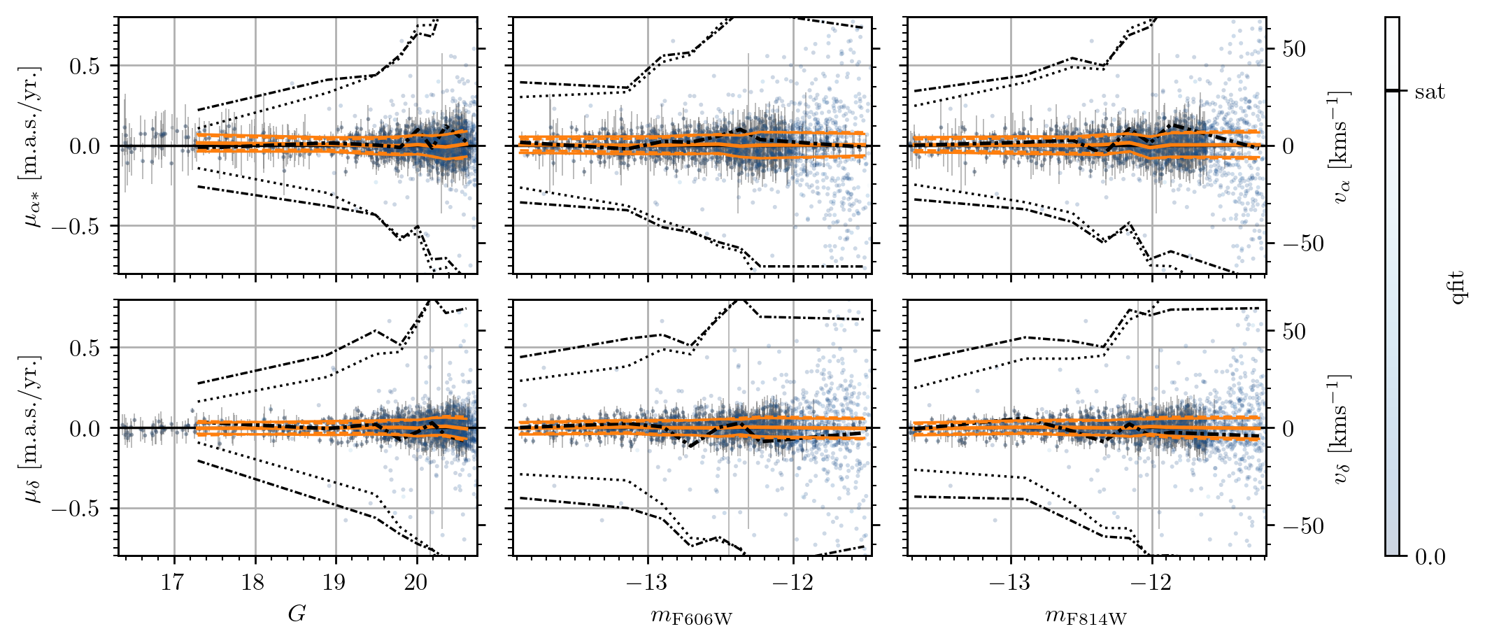
Figure 17: The relative PMs of NGC 5053 as a function of magnitude. Markers and colors coincide with those of Figure 15

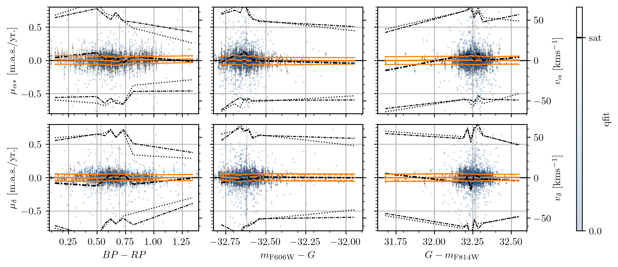
Figure 18: The relative PMs of NGC 5053 as a function of color. Markers and colors coincide with those of Figure 15.

5 GaiaHub usability

5.1 When is it a good idea to use GaiaHub?

In normal conditions, GaiaHub will always provide more precise PMs for faint stars than Gaia alone. However, the results will be limited to the field of view of HST, which will significantly reduce the number of observed stars in stellar systems larger than the covered area. This is the case in dSph galaxies and in some nearby and/or very massive GCs. Another aspect to consider is the limited magnitude range in which both instruments have common measurements, $17\leq G\leq 21$ mag (brighter stars are often saturated in HST images). This also limits the number of stars for which GaiaHub can derive PMs.

Taking these considerations into account, the usefulness of GaiaHub will generally depend on the particular scientific application. GaiaHub will provide better PM measurements on a star-by star basis, making it a very interesting tool to derive sky-projected velocity dispersions, or to find runaway stars. An ideal example case for GaiaHub would be a GC at a distance $\gtrsim 50\>{\rm kpc}$; small enough so as to fit in the HST field of view, and distant enough so its brightest RGB stars are not saturated for typical HST exposure lengths. For dSphs, GaiaHub will also provide more precise PMs, but given the small coverage of HST in these systems, their scientific usability is more limited.

In short, GaiaHub is most useful for stellar systems at distances $d_{\odot}\gtrsim 50\>{\rm kpc}$. For much closer objects, Gaia can use very bright stars that are saturated in HST images, and there is little advantage to adding HST data. For very distant objects (several hundreds of kpc), Gaia detects very few stars and HST observations alone are preferable.

5.2 Other stellar fields and uses

GaiaHub can be used in any kind of stellar field, not only stellar clusters or galaxies. However, a minimum number of at least $\sim 100$ stars is desirable to establish the reference frame. It is possible to use GaiaHub in less populated fields, although this might impact the quality of the results. If there is not a co-moving stellar population in the field of study, we strongly recommend running the code without automatic membership selection.

Lastly, GaiaHub can also be used to determine precise systemic PMs. The larger number of stars with PMs measured with GaiaHub, combined with the higher precision of the measurements compared to those of Gaia, allows for a more precise determination of systemic PMs in distant stellar systems (Bennet et al. ApJ submitted).

6 Conclusions

We have presented GaiaHub, a tool that combines HST archival images with Gaia measurements to derive precise PMs. GaiaHub boosts the scientific impact of both observatories beyond their individual capabilities by providing a second epoch observation for any HST archival image, and improving the PM accuracy for any faint source $(G\gtrsim 18)$ in the Gaia catalog observed by HST more than $\sim 6$ years ago. Our results show that random uncertainties with GaiaHub improve by roughly a factor $\Delta T_{\rm Gaia+HST}/\Delta T_{\rm Gaia}$ over those of Gaia, which is equivalent to PMs $\sim 10$ times more precise than those of Gaia EDR3 at $G=19.5$ when using HST observations taken in the year 2007. While the differences in precision between Gaia and GaiaHub will drop with future Gaia data releases, GaiaHub will always produce more precise PMs at fainter magnitudes, making it interesting for a large number of stellar systems in the Local Group. GaiaHub is completely public and accessible for everyone, and we plan to maintain it and update it.

As demonstration of its capabilities, we used GaiaHub to derive the internal PMs of 4 dSph galaxies; Draco, Sculptor, Sextans, and Fornax; and 37 globular clusters with just one HST epoch, or located at distances larger than 25 kpc. Some of the systems are located at large distances of order $100\>{\rm kpc}$. The precision achieved with GaiaHub allowed us to measure tangential velocities of individual stars with accuracies below the central velocity dispersion values in almost all the analyzed systems, e.g. $\Delta(\mu)\sim 1.3\ {\rm{mas\ yr^{-1}}}\>$ ($\sim 9.1\ {\rm{km\ s^{-1}}}\>$) at $G=19.5$ in Fornax ($\sigma(v_{\mathrm{LOS}})=11.7\pm 0.9\ {\rm{km\ s^{-1}}}\>$, $d_{\odot}=147\pm 12\>{\rm kpc}$). We used these measurements to derive the 2D sky-projected velocity dispersion values. Our results are generally consistent with those available in the literature derived from line-of-sight velocity measurements. They are also compatible with those derived using HST-only PMs, where available.

We confirm existing results for other samples that GCs tend towards mild radial velocity dispersion anisotropy. We also find that the shape of the GCs is related to their internal kinematics, with more round clusters being more isotropic than those showing smaller $\sigma(v_{\rm sky})/\sigma(v_{\mathrm{LOS}})$ ratios. Lastly, we also confirm previous findings that Draco and Sculptor appear to be radially anisotropic systems. For systems such Fornax of Sextans a longer time baseline is required in order to derive more consistent results.

Lastly, we have measured the impact of possible systematic effects in GaiaHub results following two different approaches. Results from these tests yield an all-sky median maximum error of $\widetilde{\Delta_{sys}}(\mu_{\alpha\star},\mu_{\delta})\sim(25,15)\ \mu{\rm as}\,{\rm yr}^{-1}$. We expect these systematics to improve with future Gaia data releases.

Acknowledgements: The authors thank the anonymous referee for the comments that have helped to improve this paper. Support for this work was provided by a grant for HST archival program 15633 provided by the Space Telescope Science Institute, which is operated by AURA, Inc., under NASA contract NAS 5-26555. A. del Pino acknowledges the financial support from the European Union - NextGenerationEU and the Spanish Ministry of Science and Innovation through the Recovery and Resilience Facility project J-CAVA. A. del Pino also thanks Dr. Bertran de Lis and Mr. Piñero Diaz for their support and help during the realization of this project. This work has made use of data from the European Space Agency (ESA) mission Gaia (https://www.cosmos.esa.int/gaia), processed by the Gaia Data Processing and Analysis Consortium (DPAC, https://www.cosmos.esa.int/web/gaia/dpac/consortium). Funding for the DPAC has been provided by national institutions, in particular the institutions participating in the Gaia Multilateral Agreement. This work is part of the HSTPROMO (High-resolution Space Telescope PROper MOtion) Collaboration, a set of projects aimed at improving our dynamical understanding of stars, clusters and galaxies in the nearby Universe through measurement and interpretation of proper motions from HST, Gaia, and other space observatories. We thank the collaboration members for the sharing of their ideas and software.

Software: numpy (Harris et al., 2020), scipy (Virtanen et al., 2020), matplotlib (Hunter, 2007), astropy (Astropy Collaboration et al., 2013; Price-Whelan et al., 2018),

Appendix A GaiaHub execution

GaiaHub is designed as an automatic pipeline that can run at a wide variety of user input levels. It can compute and manage all the technical nuisance parameters and steps required in order to measure PMs combining HST and Gaia data. This includes but it is not limited to: finding and downloading suitable HST images, performing astrometric measurements in these, dealing with different data quality and time baselines, dealing with saturated stars, and membership selection.

In this Appendix we provide a general guideline on how to execute GaiaHub and its available options. The best way to learn about these options is through the help included with GaiaHub;

$ gaiahub --help

.

A.1 Basic execution

GaiaHub allows users to automatically search the MAST and Gaia catalogs for suitable HST images and Gaia stars around a set of coordinates in the sky;

$ gaiahub --ra 15.03898 --dec -33.70903

.

Since no search radius was provided in the example above, GaiaHub will ask the user what radius they want to use. Another option is to search by the name of the object of interest;

$ gaiahub --name "Sculptor dSph"

.

In this case, GaiaHub will try to use the SIMBAD search engine (Wenger et al., 2000) to obtain the central coordinates $(\alpha,\delta)$ of the Sculptor dSph galaxy and its projected size in the sky. These quantities, if available, will define a cone region in the sky where GaiaHub will download the Gaia data and try to find suitable HST observations. Specifically, the search region will be centered in the object’s central coordinates and will have a radius $\mbox{\tt search\_radius}=\max(2r_{\rm ma},2)\arcdeg$, where $r_{\rm ma}$ is the length in degrees of the object’s optical major axis. Both sky coordinates and the search radius can be manually set by explicitly including the desired value during the call to GaiaHub. For example,

$ gaiahub --name "Sculptor dSph" \
--search_radius 1.2

,

will search for all suitable data in a cone of 1.2 degrees around the central coordinates of the Sculptor dSph galaxy. When providing the coordinates explicitly, these will be used instead of those found in SIMBAD. These are defined by the --ra and --dec options:

$ gaiahub --name "Sculptor dSph" \
--ra 15.05 --dec -33.84 --search_radius 0.25

.

Here, since the coordinates and --search_radius are explicitly set by the user, the option --name will only be used to create a new folder named as the object and subsequent sub folders where the results and intermediate files will be stored. If no name is provided, the folder will be named "Output".

A.1.1 Advanced execution

GaiaHub includes a wide range of options that allow the user to fine-tune their search and the way the PMs are computed. Some options are implemented as flags that can be included in the execution call in order to activate a certain feature or behavior. Other options must be followed by a string, number, or list of numbers or strings separated by a space, in order to specify the value to be used. For example,

$ gaiahub --name "Omega Cent" \
--ra 201.405 --dec -47.667 \
--search_radius 0.1 \
--hst_filters "F814W" "F606W" --use_members \
--use_sat --preselect_cmd \
--preselect_pm --use_only_good_gaia

,

will search for Gaia and HST data in a cone of 0.1 degrees around the coordinates (RA, Dec)$=(201.405,-47.667)$, but only in the F814W and F606W filters for the HST. The --use_members flag forces GaiaHub to use only member stars during the alignment between epochs, while --use_sat allows the use of saturated stars for the same purpose. The --preselect_cmd and --preselect_pm allows the user, respectively, to do an interactive manual selection of stars in the CMD and the VPD before the automatic membership selection in the PM space. Lastly, the --use_only_good_gaia flag forces GaiaHub to use only stars that have passed the quality cuts proposed in Riello et al. (2020) and Lindegren et al. (2020) to do the alignment (see Section 2.1.1 from Martínez-García et al., 2021, for more information).

The user can also chose to to run GaiaHub in a completely automatic, non-interactive way. This is done using the --quiet flag, which forces GaiaHub to adopt all default values in case some quantity was not defined during the call to the program. This is useful to execute GaiaHub within another script.

A.1.2 Modular Execution

GaiaHub consist of a main program and a module file, gaiahubmod, containing all the required functions and routines for its execution. This module can be added to the Python path and be imported into a Python session. For example the Python script

$ import gaiahubmod as gh \
obs, data = gh.search_mast(201.405, -47.667)

,

will return the tables obs and data, containing all suitable HST observations around (RA, Dec) $=(201.405^{\circ},-47.667^{\circ})$.

A.1.3 Execution times, data download and storage

The execution time of GaiaHub greatly depends on the amount of data being used, the options used, and on whether it is the first execution. Given a particular field, the first execution will normally be the slowest, as GaiaHub has to download all the data, run the detection of sources in the HST images, and then perform the actual fitting between epochs and compute the PMs. The first two steps are the most time consuming, and in cases where a large amount of HST images are being used, GaiaHub may need several minutes to download and reduce them. However, these first steps normally have to be performed just once, as GaiaHub stores data locally in the computer where it is being executed. Subsequent runs of the script will be much faster, requiring normally less than a minute in a field with 4 HST images and few hundreds of stars (as tested on a 2.8 GHz Intel Core i7 with four cores). Fields with several thousands of stars can take up to several minutes depending on the options.

If a new search is made with different coordinates or search radius, GaiaHub will then download new Gaia data and HST images if necessary. Each HST image require from around 200 Megabytes of free space in the disk, which could rapidly increase the total required free space depending on the number of images.

Appendix B Membership selection

GaiaHub performs automatic membership selection following a slightly modified version of the method described in del Pino et al. (2021). A 2D Gaussian model is fitted to the relative PMs measured by GaiaHub. The PMs and their uncertainties are then Mahalanobis whitened (ZCA) as:

$$\mu_{ZCA}=U\Lambda^{-1/2}U^{T}\mu$$ (B1)

,

where $\mu$ is the vector of the PMs and their uncertainties, $\Lambda$ are the eigenvalues of the covariance matrix, and $U$ the eigenvectors. Stars not fulfilling

$$\left(\mu_{\alpha\star,ZCA}^{2}+\mu_{\delta,ZCA}^{2}\right)^{1/2}\leq n{\rm,and}$$ (B2)

$$\left[\sigma(\mu_{\alpha\star})_{ZCA}^{2}+\sigma(\mu_{\delta})_{ZCA}^{2}\right]^{1/2}\leq n$$ (B3)

are rejected, where $n$ is the number of $\sigma$ (3 by default). A new Gaussian fit is performed on the remaining stars and the process is repeated until convergence. In cases where the method does not converges, the user can manually select stars in the CMD or in the VPD prior to their automatic selection in the PMs space.

Appendix C Gaia positional uncertainties

There is not much information about how accurate Gaia positional errors are. However, many studies have reported uncertainties in parallaxes and PMs to be underestimated. By default, GaiaHub tries to correct this by multiplying Gaia positional uncertainties by a factor 1.05 and 1.22 for 5-parameter and 6-parameter solutions, respectively (see Figure 21 in Fabricius et al., 2021). This behavior can be avoided by using the --no_error_correction, which will force GaiaHub to use the nominal positional errors listed in the gaia_source table.

References

- Amorisco & Evans (2012) Amorisco, N. C., & Evans, N. W. 2012, MNRAS, 419, 184, doi: 10.1111/j.1365-2966.2011.19684.x
- Anderson & King (2004) Anderson, J., & King, I. R. 2004, Multi-filter PSFs and Distortion Corrections for the HRC, Instrument Science Report ACS 2004-15
- Anderson & King (2006) —. 2006, PSFs, Photometry, and Astronomy for the ACS/WFC, Instrument Science Report ACS 2006-01
- Anderson & van der Marel (2010) Anderson, J., & van der Marel, R. P. 2010, ApJ, 710, 1032, doi: 10.1088/0004-637X/710/2/1032
- Antoja et al. (2018) Antoja, T., Helmi, A., Romero-Gómez, M., et al. 2018, Nature, 561, 360, doi: 10.1038/s41586-018-0510-7
- Astropy Collaboration et al. (2013) Astropy Collaboration, Robitaille, T. P., Tollerud, E. J., et al. 2013, A&A, 558, A33, doi: 10.1051/0004-6361/201322068
- Battaglia et al. (2008) Battaglia, G., Helmi, A., Tolstoy, E., et al. 2008, ApJ, 681, L13, doi: 10.1086/590179
- Battaglia et al. (2021) Battaglia, G., Taibi, S., Thomas, G. F., & Fritz, T. K. 2021, arXiv e-prints, arXiv:2106.08819. https://arxiv.org/abs/2106.08819
- Battaglia et al. (2022) —. 2022, A&A, 657, A54, doi: 10.1051/0004-6361/202141528
- Baumgardt & Hilker (2018) Baumgardt, H., & Hilker, M. 2018, MNRAS, 478, 1520, doi: 10.1093/mnras/sty1057
- Baumgardt et al. (2019) Baumgardt, H., Hilker, M., Sollima, A., & Bellini, A. 2019, MNRAS, 482, 5138, doi: 10.1093/mnras/sty2997
- Bellini et al. (2011) Bellini, A., Anderson, J., & Bedin, L. R. 2011, PASP, 123, 622, doi: 10.1086/659878
- Bellini et al. (2017) Bellini, A., Anderson, J., Bedin, L. R., et al. 2017, ApJ, 842, 6, doi: 10.3847/1538-4357/aa7059
- Bellini & Bedin (2009) Bellini, A., & Bedin, L. R. 2009, PASP, 121, 1419, doi: 10.1086/649061
- Bellini et al. (2014) Bellini, A., Anderson, J., van der Marel, R. P., et al. 2014, ApJ, 797, 115, doi: 10.1088/0004-637X/797/2/115
- Bellini et al. (2018) Bellini, A., Libralato, M., Bedin, L. R., et al. 2018, ApJ, 853, 86, doi: 10.3847/1538-4357/aaa3ec
- Belokurov et al. (2018) Belokurov, V., Erkal, D., Evans, N. W., Koposov, S. E., & Deason, A. J. 2018, MNRAS, 478, 611, doi: 10.1093/mnras/sty982
- Besla et al. (2007) Besla, G., Kallivayalil, N., Hernquist, L., et al. 2007, ApJ, 668, 949, doi: 10.1086/521385
- Bianchini et al. (2018) Bianchini, P., van der Marel, R. P., del Pino, A., et al. 2018, MNRAS, 481, 2125, doi: 10.1093/mnras/sty2365
- Brownsberger & Randall (2021) Brownsberger, S. R., & Randall, L. 2021, MNRAS, 501, 2332, doi: 10.1093/mnras/staa3719
- del Pino et al. (2015) del Pino, A., Aparicio, A., & Hidalgo, S. L. 2015, MNRAS, 454, 3996, doi: 10.1093/mnras/stv2174
- del Pino et al. (2017) del Pino, A., Aparicio, A., Hidalgo, S. L., & Łokas, E. L. 2017, MNRAS, 465, 3708, doi: 10.1093/mnras/stw3016
- del Pino et al. (2021) del Pino, A., Fardal, M. A., van der Marel, R. P., et al. 2021, ApJ, 908, 244, doi: 10.3847/1538-4357/abd5bf
- del Pino et al. (2022) del Pino, A., Libralato, M., van der Marel, R. P., et al. 2022, doi: 10.5281/zenodo.6467326
- Fabricius et al. (2021) Fabricius, C., Luri, X., Arenou, F., et al. 2021, A&A, 649, A5, doi: 10.1051/0004-6361/202039834
- Fardal et al. (2021) Fardal, M. A., van der Marel, R., del Pino, A., & Sohn, S. T. 2021, AJ, 161, 58, doi: 10.3847/1538-3881/abcccf
- Fritz et al. (2018) Fritz, T. K., Battaglia, G., Pawlowski, M. S., et al. 2018, A&A, 619, A103, doi: 10.1051/0004-6361/201833343
- Gaia Collaboration et al. (2018) Gaia Collaboration, Helmi, A., van Leeuwen, F., et al. 2018, A&A, 616, A12, doi: 10.1051/0004-6361/201832698
- Genina et al. (2018) Genina, A., Benítez-Llambay, A., Frenk, C. S., et al. 2018, MNRAS, 474, 1398, doi: 10.1093/mnras/stx2855
- Häberle et al. (2021) Häberle, M., Libralato, M., Bellini, A., et al. 2021, MNRAS, 503, 1490, doi: 10.1093/mnras/stab474
- Harris et al. (2020) Harris, C. R., Millman, K. J., van der Walt, S. J., et al. 2020, Nature, 585, 357, doi: 10.1038/s41586-020-2649-2
- Harris (1996) Harris, W. E. 1996, AJ, 112, 1487, doi: 10.1086/118116
- Helmi et al. (2018) Helmi, A., Babusiaux, C., Koppelman, H. H., et al. 2018, Nature, 563, 85, doi: 10.1038/s41586-018-0625-x
- Hunter (2007) Hunter, J. D. 2007, Computing in Science & Engineering, 9, 90, doi: 10.1109/MCSE.2007.55
- Kallivayalil et al. (2006) Kallivayalil, N., van der Marel, R. P., Alcock, C., et al. 2006, ApJ, 638, 772, doi: 10.1086/498972
- Kallivayalil et al. (2018) Kallivayalil, N., Sales, L. V., Zivick, P., et al. 2018, ApJ, 867, 19, doi: 10.3847/1538-4357/aadfee
- Libralato et al. (2019) Libralato, M., Bellini, A., Piotto, G., et al. 2019, ApJ, 873, 109, doi: 10.3847/1538-4357/ab0551
- Libralato et al. (2018) Libralato, M., Bellini, A., van der Marel, R. P., et al. 2018, ApJ, 861, 99, doi: 10.3847/1538-4357/aac6c0
- Lindegren et al. (2020) Lindegren, L., Klioner, S. A., Hernández, J., et al. 2020, Astronomy & Astrophysics
- Lindegren et al. (2021) Lindegren, L., Klioner, S. A., Hernández, J., et al. 2021, A&A, 649, A2, doi: 10.1051/0004-6361/202039709
- Martínez-García et al. (2021) Martínez-García, A. M., del Pino, A., Aparicio, A., van der Marel, R. P., & Watkins, L. L. 2021, Monthly Notices of the Royal Astronomical Society, 505, 5884, doi: 10.1093/mnras/stab1568
- Massari et al. (2018) Massari, D., Breddels, M. A., Helmi, A., et al. 2018, Nature Astronomy, 2, 156, doi: 10.1038/s41550-017-0322-y
- Massari et al. (2020) Massari, D., Helmi, A., Mucciarelli, A., et al. 2020, A&A, 633, A36, doi: 10.1051/0004-6361/201935613
- Massari et al. (2017) Massari, D., Posti, L., Helmi, A., Fiorentino, G., & Tolstoy, E. 2017, A&A, 598, L9, doi: 10.1051/0004-6361/201630174
- McConnachie (2012) McConnachie, A. W. 2012, AJ, 144, 4, doi: 10.1088/0004-6256/144/1/4
- McConnachie & Venn (2020) McConnachie, A. W., & Venn, K. A. 2020, AJ, 160, 124, doi: 10.3847/1538-3881/aba4ab
- Milone et al. (2006) Milone, A. P., Villanova, S., Bedin, L. R., et al. 2006, A&A, 456, 517, doi: 10.1051/0004-6361:20064960
- Piatek et al. (2007) Piatek, S., Pryor, C., Bristow, P., et al. 2007, AJ, 133, 818, doi: 10.1086/510456
- Piatek et al. (2008) Piatek, S., Pryor, C., & Olszewski, E. W. 2008, AJ, 135, 1024, doi: 10.1088/0004-6256/135/3/1024
- Price-Whelan et al. (2018) Price-Whelan, A. M., Sipőcz, B. M., Günther, H. M., et al. 2018, AJ, 156, 123, doi: 10.3847/1538-3881/aabc4f
- Read et al. (2021) Read, J. I., Mamon, G. A., Vasiliev, E., et al. 2021, MNRAS, 501, 978, doi: 10.1093/mnras/staa3663
- Riello et al. (2020) Riello, M., De Angeli, F., Evans, D. W., et al. 2020, arXiv e-prints, arXiv:2012.01916. https://arxiv.org/abs/2012.01916
- Ruiz-Lara et al. (2020) Ruiz-Lara, T., Gallart, C., Bernard, E. J., & Cassisi, S. 2020, Nature Astronomy, 4, 965, doi: 10.1038/s41550-020-1097-0
- Sohn et al. (2012) Sohn, S. T., Anderson, J., & van der Marel, R. P. 2012, ApJ, 753, 7, doi: 10.1088/0004-637X/753/1/7
- Sohn et al. (2018) Sohn, S. T., Watkins, L. L., Fardal, M. A., et al. 2018, ApJ, 862, 52, doi: 10.3847/1538-4357/aacd0b
- Strigari et al. (2010) Strigari, L. E., Frenk, C. S., & White, S. D. M. 2010, MNRAS, 408, 2364, doi: 10.1111/j.1365-2966.2010.17287.x
- Strigari et al. (2018) —. 2018, ApJ, 860, 56, doi: 10.3847/1538-4357/aac2d3
- van der Marel et al. (2012) van der Marel, R. P., Fardal, M., Besla, G., et al. 2012, ApJ, 753, 8, doi: 10.1088/0004-637X/753/1/8
- van der Marel et al. (2019) van der Marel, R. P., Fardal, M. A., Sohn, S. T., et al. 2019, ApJ, 872, 24, doi: 10.3847/1538-4357/ab001b
- van der Marel & Kallivayalil (2014) van der Marel, R. P., & Kallivayalil, N. 2014, ApJ, 781, 121, doi: 10.1088/0004-637X/781/2/121
- Vasiliev & Baumgardt (2021) Vasiliev, E., & Baumgardt, H. 2021, MNRAS, 505, 5978, doi: 10.1093/mnras/stab1475
- Virtanen et al. (2020) Virtanen, P., Gommers, R., Oliphant, T. E., et al. 2020, Nature Methods, 17, 261, doi: 10.1038/s41592-019-0686-2
- Walker et al. (2009) Walker, M. G., Mateo, M., & Olszewski, E. W. 2009, AJ, 137, 3100, doi: 10.1088/0004-6256/137/2/3100
- Walker et al. (2015) Walker, M. G., Olszewski, E. W., & Mateo, M. 2015, MNRAS, 448, 2717, doi: 10.1093/mnras/stv099
- Walker & Peñarrubia (2011) Walker, M. G., & Peñarrubia, J. 2011, ApJ, 742, 20, doi: 10.1088/0004-637X/742/1/20
- Watkins et al. (2015) Watkins, L. L., van der Marel, R. P., Bellini, A., & Anderson, J. 2015, ApJ, 803, 29, doi: 10.1088/0004-637X/803/1/29
- Wenger et al. (2000) Wenger, M., Ochsenbein, F., Egret, D., et al. 2000, A&AS, 143, 9, doi: 10.1051/aas:2000332