Fat–Tailed Variational Inference with Anisotropic Tail Adaptive Flows

Abstract

While fat-tailed densities commonly arise as posterior and marginal distributions in robust models and scale mixtures, they present challenges when Gaussian-based variational inference fails to capture tail decay accurately. We first improve previous theory on tails of Lipschitz flows by quantifying how the tails affect the rate of tail decay and by expanding the theory to non-Lipschitz polynomial flows. Then, we develop an alternative theory for multivariate tail parameters which is sensitive to tail-anisotropy. In doing so, we unveil a fundamental problem which plagues many existing flow-based methods: they can only model tail-isotropic distributions (i.e., distributions having the same tail parameter in every direction). To mitigate this and enable modeling of tail-anisotropic targets, we propose anisotropic tail-adaptive flows (ATAF). Experimental results on both synthetic and real-world targets confirm that ATAF is competitive with prior work while also exhibiting appropriate tail-anisotropy.

1 Introduction

Flow based methods (Papamakarios et al., 2021) have proven to be effective techniques to model complex probability densities. They compete with the state of the art on density estimation (Huang et al., 2018; Durkan et al., 2019; Jaini et al., 2020), generative modeling (Chen et al., 2019; Kingma & Dhariwal, 2018), and variational inference (Kingma et al., 2016; Agrawal et al., 2020) tasks. These methods start with a random variable $X$ having a simple and tractable distribution $\mu$, and apply a learnable transport map $f_{\theta}$ to build another random variable $Y=f_{\theta}(X)$ with a more expressive pushforward probability measure $(f_{\theta})_{\ast}\mu$ (Papamakarios et al., 2021). In contrast to the implicit distributions (Huszár, 2017) produced by generative adversarial networks (GANs), flow based methods restrict the transport map $f_{\theta}$ to be invertible and to have efficiently-computable Jacobian determinants. As a result, probability density functions can be tractably computed through direct application of a change of variables

$$p_{Y}(y)=p_{X}(f_{\theta}^{-1}(y))\left\lvert\det\left.\frac{df_{\theta}^{-1}(z)}{dz}\right|_{z=y}\right\rvert$$ (1)

While recent developments (Chen et al., 2019; Huang et al., 2018; Durkan et al., 2019) have focused primarily on the transport map $f_{\theta}$, the base distribution $\mu$ has received comparatively less investigation. The most common choice for the base distribution is standard Gaussian $\mu=\mathcal{N}(0,\matr{I})$. However, in Theorem 3.2, we show this choice results in significant restrictions to the expressivity of the model, limiting its utility for data that exhibits fat-tailed (or heavy-tailed) structure. Prior work addressing heavy-tailed flows (Jaini et al., 2020) are limited to tail-isotropic base distributions — in Proposition 3.6, we also prove flows built on these base distributions are unable to accurately model multivariate anisotropic fat-tailed structure.

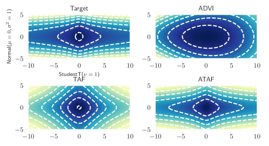
Figure 1: Variational inference against a tail-anisotropic target distribution $\mathcal{N}(0,1)\otimes\text{StudentT}(\nu=1)$ (top left). Only ATAF (bottom right) is able to correctly reproduce the tail-anisotropy (fat-tailed along $x$-axis, Gaussian along $y$-axis). In contrast, ADVI’s (top right) Gaussian base distribution and TAF’s (bottom left) tail-isotropic $\prod_{i=1}^{2}\text{StudentT}(\nu)$ base distribution can only model tail-isotropic distributions (Proposition 3.6) which erroneously imposes power-law tails with the same rate of decay along both the $x$ and $y$ axes.

Our work here aims to identify and address these deficiencies. To understand the impact of the base distribution $\mu$ in flow-based models, we develop and apply theory for fat-tailed random variables and their transformations under Lipschitz-continuous functions. Our approach leverages the theory of concentration functions (Ledoux, 2001, Chapter 1.2) to significantly sharpen and extend prior results (Jaini et al., 2019, Theorem 4) by precisely describing the tail parameters of the pushforward distribution $(f_{\theta})_{\ast}\mu$ under both Lipschitz-continuous (Theorem 3.2) and polynomial (Corollary 3.4) transport maps. In the multivariate setting, we develop a theory of direction-dependent tail parameters (Definition 3.5), and show that tail-isotropic base distributions yield tail-isotropic pushforward measures (Proposition 3.6). As a consequence of Proposition 3.6, prior methods (Jaini et al., 2020) are limited in that they are unable to capture tail-anisotropy. This motivates the construction of anisotropic tail adaptive flows (ATAF, Definition 3.7) as a means to alleviate this issue (Remark 3.8) and improve modeling of tail-anisotropic distributions. Our experiments show ATAF exhibits correct tail behaviour in synthetic target distributions exhibiting fat-tails (Figure 4) and tail-anisotropy (Figure 1). On realistic targets, we find that ATAF can yield improvements in variational inference (VI) by capturing potential tail-anisotropy (Section 4).

Related Work

Fat-tails in variational inference.

Recent work in variational autoencoders (VAEs) have considered relaxing Gaussian assumptions to heavier-tailed distributions (Mathieu et al., 2019; Chen et al., 2019; Boenninghoff et al., 2020; Abiri & Ohlsson, 2020). In (Mathieu et al., 2019), a StudentT prior distribution $p(z)$ is considered over the latent code $z$ in a VAE with Gaussian encoder $q(z\mid x)$. They argue that the anisotropy of a StudentT product distribution leads to more disentangled representations as compared to the standard choice of Normal distributions. A similar modification is performed in (Chen et al., 2020), for a coupled VAE (see (Cao et al., 2019)). It showed improvements in the marginal likelihoods of reconstructed images. In addition, Boenninghoff et al. (2020) consider a mixture of StudentTs for the prior $p(z)$. To position our work in context, note that the encoder $q(z\mid x)$ may be viewed as a variational approximation to the posterior $p(z\mid x)$ defined by the decoder model $p(x\mid z)$ and the prior $p(z)$. Our work differs from (Mathieu et al., 2019; Chen et al., 2020; Boenninghoff et al., 2020) in that we consider fat-tailed variational approximations $q(z\mid x)$ rather than priors $p(z)$. Although (Abiri & Ohlsson, 2020) also considers a StudentT approximate posterior, our work involves a more general variational family which use normalizing flows. Similarly, although (Wang et al., 2018) also deals with fat-tails in variational inference, their goal is to improve $\alpha$-divergence VI by controlling the moments of importance sampling ratios (which may be heavy-tailed). Our work here adopts Kullback-Leibler divergence and is concerned with enriching the variational family to include anisotropic fat-tailed distributions. More directly comparable recent work (Ding et al., 2011; Futami et al., 2017) studies the $t$-exponential family variational approximation which includes StudentTs and other heavier-tailed densities. Critically, the selection of their parameter $t$ (directly related to the StudentT’s degrees of freedom $\nu$), and the issue of tail anisotropy, are not discussed.

Flow based methods.

Normalizing flows and other flow based methods have a rich history within variational inference (Kingma et al., 2016; Rezende & Mohamed, 2015; Agrawal et al., 2020; Stefan Webb & Goodman, 2019). Consistent with our experience (Figure 3), (Stefan Webb & Goodman, 2019) documents normalizing flows can offer improvements over ADVI and NUTS across thirteen different Bayesian linear regression models from (Gelman & Hill, 2006). Agrawal et al. (2020) shows that normalizing flows compose nicely with other advances in black-box VI (e.g., stick the landing, importance weighting). However, none of these works treat the issue of fat-tailed targets and inappropriate tail decay. To our knowledge, only TAFs (Jaini et al., 2020) explicitly consider flows with tails heavier than Gaussians. Our work here can be viewed as a direct improvement of Jaini et al. (2020), and we make extensive comparison to this work throughout the body of this paper. At a high level, we provide a theory for fat-tails which is sensitive to the rate of tail decay and develop a framework to characterize and address the tail-isotropic limitations plaguing TAFs.

2 Flow-based methods for fat-tailed variational inference

2.1 Flow-based VI methods

The objective of VI is to approximate a target distribution $\pi(x)$ by searching over a variational family $\mathcal{Q}=\{q_{\phi}:\phi\in\Phi\}$ of probability distributions $q_{\phi}$. While alternatives exist (Li & Turner, 2016; Wang et al., 2018), VI typically seeks to find $q_{\phi}$ “close” to $\pi$ as measured by Kullback-Leibler divergence $D(q_{\phi}\;\|\;\pi)$. To ensure tractability without sacrificing generality, in practice (Wingate & Weber, 2013; Ranganath et al., 2014) a Monte-Carlo approximation of the evidence lower bound (ELBO) is maximized:

$$\text{ELBO}(\phi) =\int q_{\phi}(x)\log\frac{\bar{\pi}(x)}{q_{\phi}(x)}dx$$

$$\approx\frac{1}{n}\sum_{i=1}^{n}\log\frac{\bar{\pi}(x_{i})}{q_{\phi}(x_{i})},\;x_{i}\overset{\text{iid}}{\sim}q_{\phi},\;\bar{\pi}\propto\pi$$

To summarize, this procedure enables tractable black-box VI by replacing $\pi$ with $\bar{\pi}\propto\pi$ and approximating expectations with respect to $q_{\phi}$ (which are tractable only in simple variational families) through Monte-Carlo approximation. In Bayesian inference and probabilistic programming applications, the target posterior $\pi(x)=p(x\mid y)=\frac{p(x,y)}{p(y)}$ is typically intractable but $\bar{\pi}(x)=p(x,y)$ is computable (i.e. represented by the probabilistic program’s generative / forward execution).

Model	Autoregressive transform	Suff. conditions for Lipschitz
NICE(Dinh et al., 2014)	$z_{j}+\mu_{j}\cdot\mathds{1}_{k\not\in[j]}$	$\mu_{j}$ Lipschitz
MAF(Papamakarios et al., 2017)	$\sigma_{j}z_{j}+(1-\sigma_{j})\mu_{j}$	$\sigma_{j}$ bounded
IAF(Kingma et al., 2016)	$z_{j}\cdot\exp(\lambda_{j})+\mu_{j}$	$\lambda_{j}$ bounded, $\mu_{j}$ Lipschitz
Real-NVP(Dinh et al., 2016)	$\exp(\lambda_{j}\cdot\mathds{1}_{k\not\in[j]})\cdot z_{j}+\mu_{j}\cdot\mathds{1}_{k\not\in[j]}$	$\lambda_{j}$ bounded, $\mu_{j}$ Lipschitz
Glow(Kingma & Dhariwal, 2018)	$\sigma_{j}\cdot z_{j}+\mu_{j}\cdot\mathds{1}_{k\not\in[j]}$	$\sigma_{j}$ bounded, $\mu_{j}$ Lipschitz
NAF(Huang et al., 2018)	$\sigma^{-1}(w^{\top}\cdot\sigma(\sigma_{j}z_{j}+\mu_{j}))$	Always (logistic mixture CDF)
NSF(Durkan et al., 2019)	$z_{j}\mathds{1}_{z_{j}\not\in[-B,B]}+M_{j}(z_{j};z_{<j})\mathds{1}_{x_{j}\in[-B,B]}$	Always (linear outside $[-B,B]$)
FFJORD(Grathwohl et al., 2018)	n/a (not autoregressive)	Always (required for invertibility)
ResFlow(Chen et al., 2019)	n/a (not autoregressive)	Always (required for invertibility)

Table 1: Some popular / recently developed flows, the autoregressive transform used in the flow (if applicable), and sufficient conditions conditions for Lipschitz-continuity. A subset of this table was first presented in (Jaini et al., 2020). $M(\cdot)$ denotes monotonic rational quadratic splines (Durkan et al., 2019).

While it is possible to construct a variational family $\mathcal{Q}$ tailored to a specific task, we are interested in VI methods which are more broadly applicable and convenient to use: $\mathcal{Q}$ should be automatically constructed from introspection of a given probabilistic model/program. Automatic differentiation variational inference (ADVI) (Kucukelbir et al., 2017) is an early implementation of automatic VI and it is still the default in certain probabilistic programming languages (Carpenter et al., 2017). ADVI uses a Gaussian base distribution $\mu$ and a transport map $f_{\theta}=f\circ\Phi_{\text{Affine}}$ comprised of an invertible affine transform composed with a deterministic transformation $f$ from $\mathbb{R}$ to the target distribution’s support (e.g., $\exp:\mathbb{R}\to\mathbb{R}_{\geq 0}$, $\text{sigmoid}:\mathbb{R}\to[0,1]$). As Gaussians are closed under affine transformations, ADVI’s representational capacity is limited to deterministic transformations of Gaussians. Hence it cannot represent complex multi-modal distributions. To address this, more recent work (Kingma et al., 2016; Stefan Webb & Goodman, 2019) replaces the affine map $\Phi_{\text{Affine}}$ with a flow $\Phi_{\text{Flow}}$ typically parameterized by an invertible neural network:

Definition 2.1.

ADVI (with normalizing flows) comprise the variational family $\mathcal{Q}_{\text{ADVI}}~{}\coloneqq~{}\{(f~{}\circ~{}\Phi_{\text{Flow}})_{\ast}\mu\}$ where $\mu=\text{Normal}(0_{d},I_{d})$, $\Phi_{\text{Flow}}$ is an invertible flow transform (e.g., Table 1) and $f$ is a deterministic bijection between constrained supports (Kucukelbir et al., 2017).

As first noted in (Jaini et al., 2020), the pushforward of a light-tailed Gaussian base distribution under a Lipschitz-continuous flow will remain light-tailed and provide poor approximation to fat-tailed targets. Despite this, many major probabilistic programming packages still make a default choice of Gaussian base distribution (AutoNormalizingFlow/AutoIAFNormal in Pyro (Bingham et al., 2019), method=variational in Stan (Carpenter et al., 2017), NormalizingFlowGroup in PyMC (Patil et al., 2010)). To address this issue, tail-adaptive flows (Jaini et al., 2020) use a base distribution $\mu_{\nu}=\prod_{i=1}^{d}\text{StudentT}(\nu)$ where a single degrees-of-freedom $\nu\in\mathbb{R}$ is used across all $d$ dimensions. More precisely,

Definition 2.2.

Tail adaptive flows (TAF) comprise the variational family $\mathcal{Q}_{\text{TAF}}\coloneqq\{(f\circ\Phi_{\text{Flow}})_{\ast}\mu_{\nu}\}$ where $\mu_{\nu}=\prod_{i=1}^{d}\text{StudentT}(\nu)$ with $\nu$ shared across all $d$ dimensions, $\Phi_{\text{Flow}}$ is an invertible flow, and $f$ is a bijection between constrained supports (Kucukelbir et al., 2017). During training, the shared degrees of freedom $\nu$ is treated as an additional variational parameter.

2.2 Fat-tailed variational inference

Fat-tailed variational inference (FTVI) considers the setting where the target $\pi(x)$ is fat-tailed. Such distributions commonly arise during a standard “robustification” approach where light-tailed noise distributions are replaced with fat-tailed ones (Tipping & Lawrence, 2005). They also appear when weakly informative prior distributions are used in Bayesian hierarchical models (Gelman et al., 2006).

To formalize these notions of fat-tailed versus light-tailed distributions, a quantitative classification for tails is required. While prior work classified distribution tails according to quantiles and the existence of moment generating functions (Jaini et al., 2020, Section 3), here we propose a more natural and finer-grained classification based upon the theory of concentration functions (Ledoux, 2001, Chapter 1.2) which is sensitive to the rate of tail decay.

Definition 2.3 (Classification of tails).

For each $\alpha,p>0$, we let

• $\mathcal{E}_{\alpha}^{p}$ denote the set of exponential-type random variables $X$ with $\mathbb{P}(|X|\geq x)=\Theta(e^{-\alpha x^{p}})$;

• $\mathcal{L}_{\alpha}^{p}$ denote the set of logarithmic-type random variables $X$ with $\mathbb{P}(|X|\geq x)=\Theta(e^{-\alpha(\log x)^{p}})$.

In both cases, we call $p$ the class index and $\alpha$ the tail parameter for $X$. Note that every $\mathcal{E}_{\alpha}^{p}$ and $\mathcal{L}_{\beta}^{q}$ are disjoint, that is, $\mathcal{E}_{\alpha}^{p}\cap\mathcal{L}_{\beta}^{q}=\emptyset$ for all $\alpha,\beta,p,q>0$. For brevity, we define the ascending families $\overline{\mathcal{E}_{\alpha}^{p}}$ and $\overline{\mathcal{L}_{\alpha}^{p}}$ analogously as before except with $\Theta(\cdot)$ replaced by $\mathcal{O}(\cdot)$. Similarly, we denote the class of distributions with exponential-type tails with class index at least $p$ by $\overline{\mathcal{E}^{p}}=\cup_{\alpha\in\mathbb{R}_{+}}\overline{\mathcal{E}_{\alpha}^{p}}$, and similarly for $\overline{\mathcal{L}^{p}}$.

For example, $\overline{\mathcal{E}_{\alpha}^{2}}$ corresponds to $\alpha^{-1/2}$-sub-Gaussian random variables, $\overline{\mathcal{E}_{\alpha}^{1}}$ corresponds to sub-exponentials, and (of particular relevance to this paper) $\mathcal{L}^{1}_{\alpha}$ corresponds to the class of power-law distributions.

3 Tail behavior of Lipschitz flows

This section states our main theoretical contributions; proofs are deferred to Appendix A. We sharpen previous impossibility results approximating fat-tailed targets using light-tailed base distributions (Jaini et al., 2020, Theorem 4) by characterizing the effects of Lipschitz-continuous transport maps on not only the tail class but also the class index and tail parameter (Definition 2.3). Furthermore, we extend the theory to include polynomial flows (Jaini et al., 2019). For the multivariate setting, we define the tail-parameter function (Definition 3.5) to help formalize the notion of tail-isotropic distributions and prove a fundamental limitation that tail-isotropic pushforwards remain tail-isotropic (Proposition 3.6).

Most of our results are developed within the context of Lipschitz-continuous transport maps $f_{\theta}$. In practice, many flow-based methods exhibit Lipschitz-continuity in their transport map either by design (Grathwohl et al., 2018; Chen et al., 2019), or as a consequence of choice of architecture and activation function (Table 1). The following assumption encapsulates this premise.

Assumption 3.1.

$f_{\theta}$ is invertible, and both $f_{\theta}$ and $f^{-1}_{\theta}$ are $L$-Lipschitz continuous (e.g., sufficient conditions in Table 1 are satisfied).

It is worth noting that domains other than $\mathbb{R}^{d}$ may require an additional bijection between supports (e.g. $\exp:\mathbb{R}\to\mathbb{R}_{+}$) which could violate 3.1.

3.1 Closure of tail classes

Our first set of results pertain to closure of the tail classes in Definition 2.3 under Lipschitz-continuous transport maps. While earlier work (Jaini et al., 2020) demonstrated closure of exponential-type distributions $\cup_{p>0}\overline{\mathcal{E}^{p}}$ under flows satisfying 3.1, our results in Theorem 3.2, and Corollaries 3.3 and 3.4 sharpen these observations, showing that (1) Lipschitz transport maps cannot decrease the class index $p$ for exponential-type random variables, but can alter the tail parameter $\alpha$; and (2) under additional assumptions, cannot change either class index $p$ or the tail parameter $\alpha$ for logarithmic-type random variables.

Theorem 3.2 (Lipschitz maps of tail classes).

Under 3.1, the distribution classes $\overline{\mathcal{E}^{p}}$ and $\overline{\mathcal{L}^{p}_{\alpha}}$ (with $p,\alpha>0$) are closed under every flow transformation in Table 1.

Informally, Theorem 3.2 asserts that light-tailed base distributions cannot be transformed via Lipschitz transport maps into fat-tailed target distributions. Note this does not violate universality theorems for certain flows (Huang et al., 2018) as these results only apply in the infinite-dimensional limit. Indeed, certain exponential-type families (such as Gaussian mixtures) are dense in the class of all distributions, including those that are fat-tailed.

Note that $\overline{\mathcal{L}^{p}_{\alpha}}\supset\mathcal{E}^{q}_{\beta}$ for all $p,q,\alpha,\beta$, so Theorem 3.2 by itself does not preclude transformations of fat-tailed base distributions to light-tailed targets. Under additional assumptions on $f_{\theta}$, we further establish a partial converse that a fat-tailed base distribution’s tail parameter is unaffected after pushfoward hence heavy-to-light transformations are impossible. Note here there is no ascending union over tail parameters (i.e., $\mathcal{L}^{p}_{\alpha}$ instead of $\overline{\mathcal{L}^{p}_{\alpha}}$).

Corollary 3.3 (Closure of $\mathcal{L}^{p}_{\alpha}$).

If in addition $f_{\theta}$ is smooth with no critical points on the interior or boundary of its domain, then $\mathcal{L}_{\alpha}^{p}$ is closed.

This implies that simply fixing a fat-tailed base distribution a priori is insufficient; the tail-parameter(s) of the base distribution must be explicitly optimized alongside the other variational parameters during training. While these additional assumptions may seem restrictive, note that many flow transforms explicitly enforce smoothness and monotonicity (Wehenkel & Louppe, 2019; Huang et al., 2018; Durkan et al., 2019) and hence satisfy the premises. In fact, we can show a version of Theorem 3.2 ensuring closure of exponential-type distributions under polynomial transport maps which do not satisfy 3.1. This is significant because it extends the closure results to include polynomial flows such as sum-of-squares flows (Jaini et al., 2019).

Corollary 3.4 (Closure under polynomial maps).

For any $\alpha,\beta,p,q\in\mathbb{R}_{+}$, there does not exist a finite-degree polynomial map from $\mathcal{E}_{\alpha}^{p}$ into $\mathcal{L}_{\beta}^{q}$.

3.2 Multivariate fat-tails and anisotropic tail adaptive flows

Next, we restrict attention to power-law tails $\mathcal{L}^{1}_{\alpha}$ and develop a multivariate fat-tailed theory and notions of isotropic/anisotropic tail indices. Using our theory, we prove that both ADVI and TAF are fundamentally limited because they are only capable of fitting tail-isotropic target measures (Proposition 3.6). We consider anisotropic tail adaptive flows (ATAF): a density modeling method which can represent tail-anisotropic distributions (Remark 3.8).

For example, consider the target distribution shown earlier in Figure 1 formed as the product of $\mathcal{N}(0,1)$ and $\text{StudentT}(\nu=1)$ distributions. The marginal/conditional distribution along a horizontal slice (e.g., the distribution of $\braket{X,e_{0}}$) is fat-tailed, while along a vertical slice (e.g., $\braket{X,e_{1}}$) it is Gaussian. Another extreme example of tail-anisotropy where the tail parameter for $\braket{X,v}$ is different in every direction $v\in\mathcal{S}^{1}$ is given in Figure 2. Here $\mathcal{S}^{d-1}$ denotes the $(d-1)$-sphere in $d$ dimensions. Noting that the tail parameter depends on the choice of direction, we are motivated to consider the following direction-dependent definition of multivariate tail parameters.

Definition 3.5.

For a $d$-dimensional random vector $X$, its tail parameter function $\alpha_{X}:\mathcal{S}^{d-1}\to\bar{\mathbb{R}}_{+}$ is defined as $\alpha_{X}(v)=-\lim_{x\to\infty}\log\mathbb{P}(\braket{v,X}\geq x)/\log x$ when the limit exists, and $\alpha_{X}(v)=+\infty$ otherwise. In other words, $\alpha_{X}(v)$ maps directions $v$ into the tail parameter of the corresponding one-dimensional projection $\braket{v,X}$. The random vector $X$ is tail-isotropic if $\alpha_{X}(v)\equiv c$ is constant and tail-anisotropic if $\alpha_{X}(v)$ is not constant but bounded.

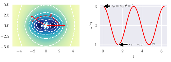
Figure 2: Illustration of the direction-dependent tail-parameter function (bottom) on a tail-anisotropic distribution (top) with PDF $\mathrm{d}P(r,\theta)=r^{-\alpha(\theta)}r\mathrm{d}r\mathrm{d}\theta$ and tail parameter $\alpha(\theta)=2+\cos(2\theta)$. While prior fat-tailed theory based on $\|X\|_{2}=\sup_{\|v\|_{2}=1}\braket{X,v}$ is only sensitive to the largest tail parameter $\max_{\theta\in[0,2\pi]}\alpha(\theta)=3.0$, our direction-dependent tail parameter function (bottom, red line) and its values along the standard basis axes ($\alpha(0)$ and $\alpha(\pi/2)$) capture tail-anisotropy.

Of course, one can construct pathological densities where this definition is not effective (see Appendix D), but it will suffice for our purposes. It is illustrative to contrast with the theory presented for TAF (Jaini et al., 2020) where only the tail exponent of $\|X\|_{2}$ is considered. For $X=(X_{1},\ldots,X_{d})$ with $X_{i}\in\mathcal{L}^{1}_{\alpha_{i}}$, by Fatou-Lebesgue and Lemma A.1

$$\mathbb{P}[\|X\|_{2}\geq t]=\mathbb{P}\left[\sup_{z\in\mathcal{S}^{d-1}}\braket{X,z}\geq t\right]$$

$$\quad\geq\sup_{z\in\mathcal{S}^{d-1}}\mathbb{P}[\braket{X,z}\geq t]=\max_{1\leq i\leq d}\nu_{i}=\max_{0\leq i\leq d-1}\alpha_{X}(e_{i})$$

Therefore, considering only the tail exponent of $\|X\|_{2}$ is equivalent to summarizing $\alpha_{X}(\cdot)$ by an upper bound. Given the absence of the tail parameters for other directions (i.e., $\alpha_{X}(v)\neq\sup_{\|v\|=1}\alpha_{X}(v)$) in the theory for TAF (Jaini et al., 2020), it should be unsurprising that both their multivariate theory as well as their experiments only consider tail-isotropic distributions obtained either as an elliptically-contoured distribution with fat-tailed radial distribution or $\prod_{i=1}^{d}\text{StudentT}(\nu)$ (tail-isotropic by Lemma A.1). Our next proposition shows that this presents a significant limitation when the target distribution is tail-anisotropic.

Proposition 3.6 (Pushforwards of tail-isotropic distributions).

Let $\mu$ be tail isotropic with non-integer parameter $\nu$ and suppose $f_{\theta}$ satisfies 3.1. Then $(f_{\theta})_{\ast}\mu$ is tail isotropic with parameter $\nu$.

To work around this limitation without relaxing 3.1, it is evident that tail-anisotropic base distributions $\mu$ must be considered. Perhaps the most straightforward modification to incorporate a tail-anisotropic base distribution replaces TAF’s isotropic base distribution $\prod_{i=1}^{d}\text{StudentT}(\nu)$ with $\prod_{i=1}^{d}\text{StudentT}(\nu_{i})$. Note that $\nu$ is no longer shared across dimensions, enabling $d$ different tail parameters to be represented:

Definition 3.7.

Anisotropic Tail-Adaptive Flows (ATAF) comprise the variational family $\mathcal{Q}_{\text{ATAF}}~{}\coloneqq~{}\{(f\circ\Phi_{\text{Flow}})_{\ast}\mu_{\nu}\},$ where $\mu_{\nu}=\prod_{i=1}^{d}\text{StudentT}(\nu_{i})$, each $\nu_{i}$ is distinct, and $f$ is a bijection between constrained supports (Kucukelbir et al., 2017). Analogous to (Jaini et al., 2020), ATAF’s implementation treats $\nu_{i}$ identically to the other parameters in the flow and jointly optimizes over them.

Remark 3.8.

Anisotropic tail-adaptive flows can represent tail-anisotropic distributions with up to $d$ different tail parameters while simultaneously satisfying 3.1. For example, if $\Phi_{\text{Flow}}=\text{Identity}$ and $\mu_{\nu}=\prod_{i=1}^{d}\text{StudentT}(i)$ then the pushforward $(\Phi_{\text{Flow}})_{\ast}\mu_{\nu}=\mu_{\nu}$ is tail-anisotropic.

Naturally, there are other parameterizations of the tail parameters $\nu_{i}$ that may be more effective depending on the application. For example, in high dimensions, one might prefer not to allow for $d$ unique indices, but perhaps only fewer. On the other hand, by using only $d$ tail parameters, an approximation error will necessarily be incurred when more than $d$ different tail parameters are present. Figure 2 presents a worst-case scenario where the target distribution has a continuum of tail parameters. In theory, this density could itself be used as an underlying base distribution, although we have not found this to be a good option in practice. The key takeaway is that to capture several different tails in the target density, one must consider a base distribution that incorporates sufficiently many distinct tail parameters.

Concerning the choice of StudentT families, we remark that since $\text{StudentT}(\nu)\Rightarrow\mathcal{N}(0,1)$ as $\nu\to\infty$, ATAF should still provide reasonably good approximations to target distributions in $\overline{\mathcal{E}^{2}}$ by taking $\nu$ sufficiently large. This can be seen in practice in Appendix C.

4 Experiments

Here we validate ATAF’s ability to improve a range of probabilistic modeling tasks. Prior work (Jaini et al., 2020) demonstrated improved density modelling when fat tails are considered, and our experiments are complementary by evaluating TAFs and ATAFs for variational inference tasks as well as demonstrating the effect of tail-anisotropy for modelling real-world financial returns and insurance claims datasets. We implement using the REDACTED FOR REVIEW probabilistic programming language[REDACTED] and the REDACTED FOR REVIEW library for normalizing flows[REDACTED], and we have open-sourced code for reproducing experiments[REDACTED, reviewers please see supplementary materials for code]. Additional details for the experiments are detailed in Appendix E.

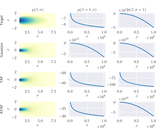
Figure 3: Bayesian linear regression’s tail-anisotropic posterior (top left) exhibits a fat-tailed conditional in $\sigma$ (as evidenced by the convex power-law decay in the top middle panel) and a Gaussian conditional in $\beta$ (concave graph in top right panel). While all methods appear to provide a good approximation of the bulk (left column), Proposition 3.6 implies Gaussian (Gaussian, second row) or isotropic StudentT product (TAF, third row) base distribution yields Gaussian or power-law tails respectively for both $\sigma$ and $\beta$. In contrast, ATAF (bottom row) illustrates Remark 3.8 by simultaneously modeling a power-law tail on $\sigma$ and Gaussian tail on $\beta$.

	ELBO	$\log p(y)$
ADVI	$\mathbf{2873.90}\pm 6.95$	$2969.73\pm 1.73$
TAF	$2839.64\pm 9.10$	$2973.85\pm 0.87$
ATAF	$2842.75\pm 8.83$	$\mathbf{2976.75}\pm 0.66$
NUTS	n/a	$3724.59\pm 0.036$

(a) diamonds

	ELBO	$\log p(y)$
ADVI	$-72.13\pm 6.89$	$-53.25\pm 3.44$
TAF	$-64.64\pm 4.88$	$-52.51\pm 4.41$
ATAF	$\mathbf{-58.63}\pm 4.75$	$\mathbf{-51.01}\pm 3.71$
NUTS	n/a	$-47.78\pm 0.093$

(b) Eight schools

Table 2: Monte-Carlo ELBO and importance weighted Monte-Carlo marginal likelihood $p(y)=\mathbb{E}_{x\sim q_{\theta}}\frac{p(x,y)}{q_{\theta}(x)}$ (higher is better, $\pm$ standard errors) estimates from VI on real-world datasets. To understand the variational approximation gap, we include marginal likelihoods based on “golden samples” from posteriordb (Developers, 2021) computed using No-U-Turn-Sampling (NUTS) (Hoffman & Gelman, 2014; Carpenter et al., 2017).

	Fama-French 5 Industry Daily	CMS 2008-2010 DE-SynPUF
ADVI	$-5.018\pm 0.056$	$-1.883\pm 0.012$
TAF	$-4.703\pm 0.023$	$-1.659\pm 0.004$
ATAF	$\mathbf{-4.699}\pm 0.024$	$\mathbf{-1.603}\pm 0.034$

Table 3: Log-likelihoods (higher is better, $\pm$ standard errors) achieved on density modeling tasks involving financial returns (Fama & French, 2015) and insurance claims (CMS, 2010) data.

4.1 Bayesian linear regression

Consider one-dimensional Bayesian linear regression (BLR) with conjugate priors, defined by priors and likelihood

$$\sigma^{2}\sim\text{Inv-Gamma}(a_{0},b_{0})$$

$$\beta\mid\sigma^{2}\sim\mathcal{N}(0,\sigma^{2}),\qquad y\mid X,\beta,\sigma\sim\mathcal{N}(X\beta,\sigma^{2})$$

where $a_{0}$, $b_{0}$ are hyperparameters and the task is to approximate the posterior distribution $p(\beta,\sigma^{2}\mid X,y)$. Owing to conjugacy, the posterior distribution can be explicitly computed. Indeed, $p(\beta,\sigma^{2}\mid X,y)=\rho(\sigma^{2})\rho(\beta\mid\sigma)$ where $\rho(\beta\mid\sigma)=\mathcal{N}(\Sigma_{n}(X^{\top}X\hat{\beta}),\sigma^{2}\Sigma_{n})$, $\Sigma_{n}=(X^{\top}X+\sigma^{-2})^{-1}$, $\hat{\beta}=(X^{\top}X)^{-1}X^{\top}y$, and

$$\rho(\sigma^{2})=\text{Inv-Gamma}\bigg{(}a_{0}+\frac{n}{2},b_{0}+\frac{1}{2}(y^{\top}y-\mu_{n}^{\top}\Sigma_{n}\mu_{n})\bigg{)}$$

This calculation reveals that the posterior distribution is tail-anisotropic: for fixed $c$ we have that $p(\sigma^{2},\beta=c\mid X,y)\propto\rho(\sigma^{2})\in\mathcal{L}^{1}_{\alpha_{n}}$ as a function of $\sigma$ (with $\alpha_{n}$ a function of $n$) and $p(\sigma^{2}=c,\beta\mid X,y)\propto\rho(\beta\mid c)\in\overline{\mathcal{E}^{2}}$ as a function of $\beta$. As a result of Proposition 3.6, we expect ADVI and TAF to erroneously impose Gaussian and power-law tails respectively for both $\beta$ and $\sigma^{2}$ as neither method can produce a tail-anisotropic pushforward. This intuition is confirmed in Figure 3, where we see that only ATAF is the only method capable of modeling the tail-anisotropy present.

Conducting Bayesian linear regression is among the standard tasks requested of a probabilistic programming language, yet still displays tail-anisotropy. To accurately capture large quantiles, this tail-anisotropy should not be ignored, necessitating a method such as ATAF.

4.2 Diamond price prediction using non-conjugate Bayesian regression

Without conjugacy, the BLR posterior is intractable and there is no reason a priori to expect tail-anisotropy. Regardless, this presents a realistic and practical scenario for evaluating ATAF’s ability to improve VI. For this experiment, we consider BLR on the diamonds dataset (Wickham, 2011) included in posteriordb (Developers, 2021). This dataset contains a covariate matrix $X\in\mathbb{R}^{5000\times 24}$ consisting of $5000$ diamonds each with $24$ features as well as an outcome variable $y\in\mathbb{R}^{5000}$ representing each diamond’s price. The probabilistic model for this inference task is specified in Stan code provided by (Developers, 2021) and is reproduced for convenience

$$\alpha\sim\text{StudentT}(\nu=3,\text{loc}=8,\text{scale}=10)$$

$$\sigma\sim\text{HalfStudentT}(\nu=3,\text{loc}=0,\text{scale}=10)$$

$$\beta\sim\mathcal{N}(0,\matr{I}_{24}),\qquad y\sim\mathcal{N}(\alpha+X\beta,\sigma)$$

For each VI method, we performed 100 trials each consisting of 5000 descent steps on the Monte-Carlo ELBO estimated using 1000 samples and report the results in Figure 4(a). We report both the final Monte-Carlo ELBO as well as a Monte-Carlo importance-weighted approximation to the log marginal likelihood $\log p(y)=\log\mathbb{E}_{x\sim q_{\theta}}\frac{p(x,y)}{q_{\theta}(y)}$ both estimated using 1000 samples.

4.3 Eight schools SAT score modelling with fat-tailed scale mixtures

The eight-schools model (Rubin, 1981; Gelman et al., 2013) is a classical Bayesian hierarchical model used originally to consider the relationship between standardized test scores and coaching programs in place at eight schools. A variation utilizing half Cauchy non-informative priors (Gelman et al., 2006) provides a real-world inference problem involving fat-tailed distributions, and is formally specified by the probabilistic model

$$\tau\sim\text{HalfCauchy}(\text{loc}=0,\text{scale}=5)$$

$$\mu\sim\mathcal{N}(0,5),\qquad\theta\sim\mathcal{N}(\mu,\tau),\qquad y\sim\mathcal{N}(\theta,\sigma)$$

Given test scores and standard errors $\{(y_{i},\sigma_{i})\}_{i=1}^{8}$, we are interested in the posterior distribution over treatment effects $\theta_{1},\ldots,\theta_{d}$. The experimental parameters are identical to Section 4.2 and results are reported in Figure 4(b).

4.4 Financial and actuarial applications

To examine the advantage of tail-anisotropic modelling in practice, we considered two benchmark datasets from financial (daily log returns for five industry indices during 1926–2021, (Fama & French, 2015)) and actuarial (per-patient inpatient and outpatient cumulative Medicare/Medicid (CMS) claims during 2008–2010, (CMS, 2010)) applications where practitioners actively seek to model fat-tails and account for black-swan events. Identical flow architectures and optimizers were used in both cases, with log-likelihoods presented in Table 3. Both datasets exhibited superior fits after allowing for heavier tails, with a further improved fit using ATAF for the CMS claims dataset.

5 Conclusion

In this work, we have sharpened existing theory for approximating fat-tailed distributions with normalizing flows, and formalized tail-(an)isotropy through a direction-dependent tail parameter. With this, we have shown that many prior flow-based methods are inherently limited by tail-isotropy. With this in mind, we proposed a simple flow-based method capable of modeling tail-anisotropic targets. As we have seen, anisotropic FTVI is already applicable in fairly elementary examples such as Bayesian linear regression and ATAFs provide one of the first methods for using the representational capacity of flow-based methods while simultaneously producing tail-anisotropic distributions. A number of open problems still remain, including the study of other parameterizations of the tail behaviour of the base distribution. Even so, going forward, it seems prudent that density estimators, especially those used in black-box settings, consider accounting for tail-anisotropy using a method such as ATAF.

Appendix A Proofs

Proof of Theorem 3.2.

Let $X$ be a random variable from either $\mathcal{E}_{\alpha}^{p}$ or $\mathcal{L}_{\alpha}^{p}$. Its concentration function (Equation 1.6 (Ledoux, 2001) is given by

$$\alpha_{X}(r)\coloneqq\sup\{\mu\{x:d(x,A)\geq r\};A\subset\text{supp}~{}X,\mu(A)\geq 1/2\}=\mathbb{P}(\lvert X-m_{X}\rvert\geq r)$$

Under Assumption 1, $f_{\theta}$ is Lipschitz (say with Lipschitz constant $L$) so by Proposition 1.3 of (Ledoux, 2001),

$$\mathbb{P}(\lvert f_{\theta}(X)-m_{f_{\theta}(X)}\rvert\geq r)\leq 2\alpha_{X}(r/L)=\mathcal{O}(\alpha_{X}(r/L)),$$

where $m_{f_{\theta}(X)}$ is a median of $f_{\theta}(X)$. Furthermore, by the triangle inequality

$$\mathbb{P}(\lvert f_{\theta}(X)\rvert\geq r) =\mathbb{P}(\lvert f_{\theta}(X)-m_{f_{\theta}(X)}+m_{f_{\theta}(X)}\rvert\geq r)$$

$$\leq\mathbb{P}(\lvert f_{\theta}(X)-m_{f_{\theta}(X)}\rvert\geq r-\lvert m_{f_{\theta}(X)}\rvert)$$

$$=\mathcal{O}(\mathbb{P}(\lvert f_{\theta}(X)-m_{f_{\theta}(X)}\rvert\geq r))$$

$$=\mathcal{O}(\alpha_{X}(r/L))$$ (2)

where the asymptotic equivalence holds because $\lvert m_{f_{\theta}(X)}\rvert$ is independent of $r$. When $X\in\mathcal{E}_{\alpha}^{p}$, Equation 2 implies

$$\mathbb{P}(\lvert f_{\theta}(X)\rvert\geq r)=\mathcal{O}(e^{-\frac{\alpha}{L}r^{p}})\implies f_{\theta}(X)\in\overline{\mathcal{E}}_{\alpha/L}^{p},$$

from whence we find that the Lipschitz transform of exponential-type tails continues to possess exponential-type tails with the same class index $p$, although the tail parameter may have changed. Hence, $\overline{\mathcal{E}^{p}}$ is closed under Lipschitz maps for each $p\in\mathbb{R}_{>0}$. On the other hand, when $X\in\mathcal{L}_{\alpha}^{p}$, Equation 2 also implies that

$$\mathbb{P}(\lvert f_{\theta}(X)\rvert\geq r) =\mathcal{O}(e^{-\alpha(\log(r/L))^{p}})=\mathcal{O}(e^{-\alpha(\log r)^{p}}),$$

and therefore, $f_{\theta}(X)\in\overline{\mathcal{L}_{\alpha}^{p}}$. Unlike exponential-type tails, Lipschitz transforms of logarithmic-type tails not only remain logarithmic, but their tails decay no slower than a logarithmic-type tail of the same class index with the same tail parameter $\alpha$. This upper bound suffices to show closure under Lipschitz maps for the ascending family $\overline{\mathcal{L}_{\alpha}^{p}}$. ∎

Proof of Corollary 3.3.

Let $f_{\theta}$ be as before with the additional assumptions. Since $f_{\theta}$ is a smooth continuous bijection, it is a diffeomorphism. Furthermore, by assumption $f_{\theta}$ has invertible Jacobian on the closure of its domain hence $\sup_{x\in\text{dom}~{}f_{\theta}}\lvert(f_{\theta})^{\prime}(x)\rvert\geq M>0$. By the inverse function theorem, $(f_{\theta})^{-1}$ exists and is a diffeomorphism with

$$\frac{d}{dx}(f_{\theta})^{-1}(x)=\frac{1}{(f_{\theta})^{\prime}((f_{\theta})^{-1}(x))}\leq\frac{1}{M}$$

Therefore, $(f_{\theta})^{-1}$ is $M^{-1}$-Lipschitz and we may apply Theorem 3.2 to conclude the desired result. ∎

Proof of Corollary 3.4.

Let $X\in\mathcal{E}^{p}_{\alpha}$. By considering sufficiently large $X$ such that leading powers dominate, it suffices to consider monomials $Y=X^{k}$. Notice $\mathbb{P}(Y\geq x)=\mathbb{P}(X\geq x^{1/k})=\Theta(e^{-\alpha x^{p/k}})$, and so $Y\in\mathcal{E}^{p/k}_{\alpha}$. The result follows by disjointness of $\mathcal{E}$ and $\mathcal{L}$. ∎

Lemma A.1.

Suppose $X\in\mathcal{L}^{1}_{\alpha}$ and $Y\in\mathcal{L}^{1}_{\beta}$. Then $X+Y\in\mathcal{L}^{1}_{\min\{\alpha,\beta\}}$.

Proof.

First, let $\gamma=\min\{\alpha,\beta\}$. It will suffice to show that (I) $\mathbb{P}(|X+Y|\geq r)=\mathcal{O}(r^{-\gamma})$, and (II) $\mathbb{P}(|X+Y|\geq r)\geq\Theta(r^{-\gamma})$. Since $(X,Y)\mapsto|X+Y|$ is a 1-Lipschitz function on $\mathbb{R}^{2}$ and $\mathbb{P}(|X|\geq r)+\mathbb{P}(|Y|\geq r)=\mathcal{O}(r^{-\gamma})$, (I) follows directly from the hypotheses and Proposition 1.11 of (Ledoux, 2001). To show (II), note that for any $M>0$, conditioning on the event $|Y|\leq M$,

$$\mathbb{P}\left(\left|X\right|+|Y|\geq r\,|\,|Y|\leq M\right)\geq\mathbb{P}\left(\left|X\right|\geq r-M\right).$$

Therefore, by taking $M$ to be sufficiently large so that $\mathbb{P}(|Y|\leq M)\geq\frac{1}{2}$,

$$\mathbb{P}\left(|X+Y|\geq r\right) \geq\mathbb{P}\left(|X|+|Y|\geq r\right)$$

$$\geq\mathbb{P}\left(\left|X\right|+|Y|\geq r\,|\,|Y|\leq M\right)\mathbb{P}\left(\left|Y\right|\leq M\right)$$

$$\geq\frac{1}{2}\mathbb{P}\left(\left|X\right|\geq r-M\right)=\Theta(r^{-\alpha}).$$

The same process with $X$ and $Y$ reversed implies $\mathbb{P}(|X+Y|\geq r)\geq\Theta(r^{-\beta})$ as well. Both (II) and the claim follow. ∎

To show Proposition 3.6, we will require a few extra assumptions to rule out pathological cases. The full content of Proposition 3.6 is contained in the following theorem.

Theorem A.2.

Suppose there exists $\nu>0$ such that $C:\mathcal{S}^{d-1}\to(0,\infty)$ satisfies $C(v)\coloneqq\lim_{x\to\infty}x^{\nu}\mathbb{P}(|\langle v,X\rangle|>x)$ for all $v\in\mathcal{S}^{d-1}$. If $\nu$ is not an integer and $f$ is a bilipschitz function, then $f(X)$ is tail-isotropic with tail index $\nu$.

Proof.

Since $x\mapsto\langle v,f(x)\rangle$ is Lipschitz continuous for any $v\in\mathcal{S}^{d-1}$, Theorem 3.2 implies $\langle v,f(X)\rangle\in\overline{\mathcal{L}_{\nu}^{1}}$. Let $\theta\in(0,\pi/2)$ (say, $\theta=\pi/4$), and let $S_{v}=\{x\,:\,\cos^{-1}(\langle x/\|x\|,v\rangle)\leq\theta\}$ for each $v\in\mathcal{S}^{d-1}$. Then

$$H_{v}\coloneqq\{x\,:\,\langle v,x\rangle>1\}\supset\{x\,:\,\|x\|>(1-\cos\theta)^{-1}\}\cap S_{v}.$$

From Theorem C.2.1 of (Buraczewski et al., 2016), since $\nu\not\in\mathbb{Z}$, there exists a non-zero measure $\mu$ such that

$$\mu(E)=\lim_{x\to\infty}\frac{\mathbb{P}(x^{-1}X\in E)}{\mathbb{P}(\|X\|>x)},$$

for any Borel set $E$. Consequently, $\mu$ is regularly varying, and so by the spectral representation of regularly varying random vectors (see p. 281 (Buraczewski et al., 2016)), there exists a measure $P$ such that

$$\lim_{x\to\infty}\frac{\mathbb{P}(\|X\|>tx,X/\|X\|\in E)}{\mathbb{P}(\|X\|>x)}=t^{-\nu}P(E),$$

for any Borel set $E$ on $\mathcal{S}^{d-1}$ and any $t>0$. Letting $F_{v}=\{y/\|y\|\,:\,f(y)\in S_{v}\}\subset\mathcal{S}^{d-1}$ (noting that $P(F_{v})>0$ by assumption), since $m\|x-y\|\leq\|f(x)-f(y)\|\leq M\|x-y\|$ for all $x,y$,

$$\liminf_{x\to\infty}\frac{\mathbb{P}(f(X)\in xH_{v})}{\mathbb{P}(\|f(X)\|>x)} \geq\liminf_{x\to\infty}\frac{\mathbb{P}(\|f(X)\|>x(1-\cos\theta)^{-1},f(X)\in S_{v})}{\mathbb{P}(\|f(X)\|>x)}$$

$$\geq\liminf_{x\to\infty}\frac{\mathbb{P}(\|X\|>x(m(1-\cos\theta))^{-1},X/\|X\|\in F_{v})}{\|X\|>x/M}$$

$$\geq P(F_{v})\left(\frac{M}{m(1-\cos\theta)}\right)^{-\nu}>0.$$

where $P(F_{v})>0$ follows from the bilipschitz condition for $f$. Therefore, we have shown that $\mathbb{P}(\langle v,f(X)\rangle>x)=\Theta(\mathbb{P}(\|f(X)\|>x))$ for every $v\in\mathcal{S}^{d-1}$. Since $\mathbb{P}(\|f(X)\|>x)$ obeys a power law with exponent $\nu$ by Corollary 3.3, $f(X)$ is tail-isotropic with exponent $\nu$. ∎

Appendix B Experiments performing VI against a fat-tailed Cauchy target

The motivation for the fat-tailed variational families used in TAF/ATAF is easily illustrated on a toy example consisting of $X\sim\text{Cauchy}(x_{0}=0,\gamma=1)\in\mathcal{L}^{1}_{1}$. As seen in Figure 4, while ADVI with normalizing flows (Kingma et al., 2016; Stefan Webb & Goodman, 2019) appears to provide a reasonable fit to the bulk of the target distribution (left panel), the improper imposition of sub-Gaussian tails results in an exponentially bad tail approximation (middle panel). As a result, samples drawn from the variational approximation fail a Kolmogorov-Smirnov goodness-of-fit test against the true target distribution much more often (right panel, smaller $p$-values imply more rejections) than a variational approximation which permits fat-tails. This example is a special case of Theorem 3.2.

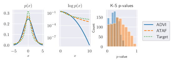
Figure 4: When performing FTVI to approximate a $X\sim\text{Cauchy}(x_{0}=0,\gamma=1)$ target (left panel, green dotted line), the use of a sub-Gaussian variational family (ADVI, solid blue line) can incur exponentially bad tail approximations (middle panel) compared to methods which permit heavier tails (ATAF, green dashed line) and results in samples which are more similar to the target (as measured by $1000$ repeats of 1-sample $N=100$ Kolmogorov-Smirnov $p$-values, right panel).

Appendix C Normal-normal location mixture

We consider a Normal-Normal conjugate inference problem where the posterior is known to be a Normal distribution as well. Here, we aim to show that ATAF performs no worse than ADVI because $\text{StudentT}(\nu)\to N(0,1)$ as $\nu\to\infty$. Figure 5 shows the resulting density approximation, which can be seen to be reasonable for both a Normal base distribution (the “correct” one) and a StudentT base distribution. This suggests that mis-specification (i.e., heavier tails in the base distribution than the target) may not be too problematic.

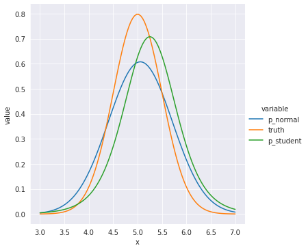
Figure 5: VI against a Normal posterior

Appendix D Example of non-existence of tail parameter due to oscillations

Consider $\text{StudentT}(\nu=1)\otimes\text{StudentT}(\nu=2)$ and “spin” it using the radial transformation $(r,\theta)\mapsto(r,r+\theta)$ (Figure 6). Due to oscillations, $\alpha_{X}(v)$ is not well defined for all $v\in\mathcal{S}^{1}$.

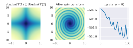
Figure 6: Taking a tail-anisotropic distribution (top) and “spinning” it (middle) results in one-dimensional projections which oscillate between tail parameters (as seen in $\log p(\braket{X,e_{0}})$ in bottom panel) and cause $\alpha_{X}(\cdot)$ to be not well defined.

Appendix E Additional details for experiments

All experiments were performed on an Intel i8700K with 32GB RAM and a NVIDIA GTX 1080 running PyTorch 1.9.0 / Python 3.8.5 / CUDA 11.2 / Ubuntu Linux 20.04 via Windows Subsystem for Linux. For all flow-transforms $\Phi_{\text{Flow}}$ we used inverse autoregressive flows (Kingma et al., 2016) with a dense autoregressive conditioner consisting of two layers of either 32 or 256 hidden units depending on problem (see code for details) and ELU activation functions. As described in (Jaini et al., 2020), TAF is trained by including $\nu$ within the Adam optimizer alongside other flow parameters. For ATAF, we include all $\nu_{i}$ within the optimizer. Models were trained using the Adam optimizer with $10^{-3}$ learning rate for 10000 iterations, which we found empirically in all our experiments to result in negligible change in ELBO at the end of training.

For Figure 4(a) and Figure 4(b), the flow transform $\Phi_{\text{Flow}}$ used for ADVI, TAF, and ATAF are comprised of two hidden layers of 32 units each. NUTS uses no such flow transform. Variational parameters for each normalizing flow were initialized using torch’s default Kaiming initialization (He et al., 2015) Additionally, the tail parameters $\nu_{i}$ used in ATAF were initialized to all be equal to the tail parameters learned from training TAF. We empirically observed this resulted in more stable results (less variation in ELBO / $\log p(y)$ across trials), which may be due to the absence of outliers when using a Gaussian base distribution resulting in more stable ELBO gradients. This suggests other techniques for handling outliers such as winsorization may also be helpful, and we leave further investigation for future work.

For Figure 3, the closed-form posterior was computed over a finite element grid to produce the “Target” row. A similar progressive training scheme used for Figure 4(a) was also used here, with the TAF flow transform $\Phi_{\text{Flow}}$ was initialized from the result of ADVI and ATAF additionally initialized all tail parameters $\nu_{i}$ based on the final shared tail parameter obtained from TAF training. Tails are computed along the $\beta=1$ or $\sigma=1$ axes because the posterior is identically zero for $\sigma=0$ hence it reveals no information about the tails.

References

- Abiri & Ohlsson (2020) Abiri, N. and Ohlsson, M. Variational auto-encoders with student’s t-prior. arXiv preprint arXiv:2004.02581, 2020.
- Agrawal et al. (2020) Agrawal, A., Sheldon, D., and Domke, J. Advances in black-box vi: Normalizing flows, importance weighting, and optimization. arXiv preprint arXiv:2006.10343, 2020.
- Bingham et al. (2019) Bingham, E., Chen, J. P., Jankowiak, M., Obermeyer, F., Pradhan, N., Karaletsos, T., Singh, R., Szerlip, P., Horsfall, P., and Goodman, N. D. Pyro: Deep universal probabilistic programming. The Journal of Machine Learning Research, 20(1):973–978, 2019.
- Boenninghoff et al. (2020) Boenninghoff, B., Zeiler, S., Nickel, R. M., and Kolossa, D. Variational autoencoder with embedded student- mixture model for authorship attribution. arXiv preprint arXiv:2005.13930, 2020.
- Buraczewski et al. (2016) Buraczewski, D., Damek, E., Mikosch, T., et al. Stochastic models with power-law tails. The equation X= AX+ B. Cham: Springer, 2016.
- Cao et al. (2019) Cao, S., Li, J., Nelson, K. P., and Kon, M. A. Coupled vae: Improved accuracy and robustness of a variational autoencoder. arXiv preprint arXiv:1906.00536, 2019.
- Carpenter et al. (2017) Carpenter, B., Gelman, A., Hoffman, M. D., Lee, D., Goodrich, B., Betancourt, M., Brubaker, M. A., Guo, J., Li, P., and Riddell, A. Stan: a probabilistic programming language. Grantee Submission, 76(1):1–32, 2017.
- Chen et al. (2020) Chen, K. R., Svoboda, D., and Nelson, K. P. Use of student’s t-distribution for the latent layer in a coupled variational autoencoder. arXiv preprint arXiv:2011.10879, 2020.
- Chen et al. (2019) Chen, R. T., Behrmann, J., Duvenaud, D., and Jacobsen, J.-H. Residual flows for invertible generative modeling. arXiv preprint arXiv:1906.02735, 2019.
- CMS (2010) CMS. Cms 2008-2010 data entrepreneurs’ synthetic public use file (de-synpuf), 2010. URL https://www.cms.gov/Research-Statistics-Data-and-Systems/Downloadable-Public-Use-Files/SynPUFs/DE_Syn_PUF.
- Developers (2021) Developers, T. S. posteriordb: a database of Bayesian posterior inference. https://github.com/stan-dev/posteriordb, 2021.
- Ding et al. (2011) Ding, N., Qi, Y., and Vishwanathan, S. t-divergence based approximate inference. Advances in Neural Information Processing Systems, 24:1494–1502, 2011.
- Dinh et al. (2014) Dinh, L., Krueger, D., and Bengio, Y. Nice: Non-linear independent components estimation. arXiv preprint arXiv:1410.8516, 2014.
- Dinh et al. (2016) Dinh, L., Sohl-Dickstein, J., and Bengio, S. Density estimation using real nvp. arXiv preprint arXiv:1605.08803, 2016.
- Durkan et al. (2019) Durkan, C., Bekasov, A., Murray, I., and Papamakarios, G. Neural spline flows. arXiv preprint arXiv:1906.04032, 2019.
- Fama & French (2015) Fama, E. F. and French, K. R. A five-factor asset pricing model. Journal of financial economics, 116(1):1–22, 2015.
- Futami et al. (2017) Futami, F., Sato, I., and Sugiyama, M. Expectation propagation for t-exponential family using q-algebra. In Advances in Neural Information Processing Systems, pp. 2245–2254, 2017.
- Gelman & Hill (2006) Gelman, A. and Hill, J. Data analysis using regression and multilevel/hierarchical models. Cambridge university press, 2006.
- Gelman et al. (2013) Gelman, A., Carlin, J. B., Stern, H. S., Dunson, D. B., Vehtari, A., and Rubin, D. B. Bayesian data analysis. CRC press, 2013.
- Gelman et al. (2006) Gelman, A. et al. Prior distributions for variance parameters in hierarchical models (comment on article by browne and draper). Bayesian analysis, 1(3):515–534, 2006.
- Grathwohl et al. (2018) Grathwohl, W., Chen, R. T., Bettencourt, J., Sutskever, I., and Duvenaud, D. Ffjord: Free-form continuous dynamics for scalable reversible generative models. arXiv preprint arXiv:1810.01367, 2018.
- He et al. (2015) He, K., Zhang, X., Ren, S., and Sun, J. Delving deep into rectifiers: Surpassing human-level performance on imagenet classification. In Proceedings of the IEEE international conference on computer vision, pp. 1026–1034, 2015.
- Hoffman & Gelman (2014) Hoffman, M. D. and Gelman, A. The no-u-turn sampler: adaptively setting path lengths in hamiltonian monte carlo. J. Mach. Learn. Res., 15(1):1593–1623, 2014.
- Huang et al. (2018) Huang, C.-W., Krueger, D., Lacoste, A., and Courville, A. Neural autoregressive flows. In International Conference on Machine Learning, pp. 2078–2087. PMLR, 2018.
- Huszár (2017) Huszár, F. Variational inference using implicit distributions. arXiv preprint arXiv:1702.08235, 2017.
- Jaini et al. (2019) Jaini, P., Selby, K. A., and Yu, Y. Sum-of-squares polynomial flow. In International Conference on Machine Learning, pp. 3009–3018. PMLR, 2019.
- Jaini et al. (2020) Jaini, P., Kobyzev, I., Yu, Y., and Brubaker, M. Tails of lipschitz triangular flows. In International Conference on Machine Learning, pp. 4673–4681. PMLR, 2020.
- Kingma & Dhariwal (2018) Kingma, D. P. and Dhariwal, P. Glow: Generative flow with invertible 1x1 convolutions. arXiv preprint arXiv:1807.03039, 2018.
- Kingma et al. (2016) Kingma, D. P., Salimans, T., Jozefowicz, R., Chen, X., Sutskever, I., and Welling, M. Improved variational inference with inverse autoregressive flow. In Advances in neural information processing systems, pp. 4743–4751, 2016.
- Kucukelbir et al. (2017) Kucukelbir, A., Tran, D., Ranganath, R., Gelman, A., and Blei, D. M. Automatic differentiation variational inference. The Journal of Machine Learning Research, 18(1):430–474, 2017.
- Ledoux (2001) Ledoux, M. The concentration of measure phenomenon. American Mathematical Soc., 2001.
- Li & Turner (2016) Li, Y. and Turner, R. E. Variational inference with rényi divergence. stat, 1050:6, 2016.
- Mathieu et al. (2019) Mathieu, E., Rainforth, T., Siddharth, N., and Teh, Y. W. Disentangling disentanglement in variational autoencoders. In International Conference on Machine Learning, pp. 4402–4412. PMLR, 2019.
- Papamakarios et al. (2017) Papamakarios, G., Pavlakou, T., and Murray, I. Masked autoregressive flow for density estimation. In Advances in Neural Information Processing Systems, pp. 2338–2347, 2017.
- Papamakarios et al. (2021) Papamakarios, G., Nalisnick, E., Rezende, D. J., Mohamed, S., and Lakshminarayanan, B. Normalizing flows for probabilistic modeling and inference. Journal of Machine Learning Research, 22(57):1–64, 2021.
- Patil et al. (2010) Patil, A., Huard, D., and Fonnesbeck, C. J. Pymc: Bayesian stochastic modelling in python. Journal of statistical software, 35(4):1, 2010.
- Ranganath et al. (2014) Ranganath, R., Gerrish, S., and Blei, D. Black box variational inference. In Artificial intelligence and statistics, pp. 814–822. PMLR, 2014.
- Rezende & Mohamed (2015) Rezende, D. and Mohamed, S. Variational inference with normalizing flows. In International Conference on Machine Learning, pp. 1530–1538. PMLR, 2015.
- Rubin (1981) Rubin, D. B. Estimation in parallel randomized experiments. Journal of Educational Statistics, 6(4):377–401, 1981.
- Stefan Webb & Goodman (2019) Stefan Webb, J. P. Chen, M. J. and Goodman, N. Improving automated variational inference with normalizing flows. 6th ICML Workshop on Automated Machine Learning (AutoML), 2019.
- Tipping & Lawrence (2005) Tipping, M. E. and Lawrence, N. D. Variational inference for student-t models: Robust bayesian interpolation and generalised component analysis. Neurocomputing, 69(1-3):123–141, 2005.
- Wang et al. (2018) Wang, D., Liu, H., and Liu, Q. Variational inference with tail-adaptive f-divergence. Advances in Neural Information Processing Systems, 31:5737–5747, 2018.
- Wehenkel & Louppe (2019) Wehenkel, A. and Louppe, G. Unconstrained monotonic neural networks. arXiv preprint arXiv:1908.05164, 2019.
- Wickham (2011) Wickham, H. ggplot2. Wiley Interdisciplinary Reviews: Computational Statistics, 3(2):180–185, 2011.
- Wingate & Weber (2013) Wingate, D. and Weber, T. Automated variational inference in probabilistic programming. arXiv preprint arXiv:1301.1299, 2013.