Sound attenuation in the hyperhoneycomb Kitaev spin liquid

Abstract

In recent years, it has been shown that the phonon dynamics may serve as an indirect probe of fractionalization of spin degrees of freedom. Here we propose that the sound attenuation measurements allows for the characterization and identification of the Kitaev quantum spin liquid on the hyperhoneycomb lattice, which is particularly interesting since the strong Kitaev interaction was observed in the the hyperhoneycomb magnet $\beta$-Li₂IrO₃. To this end we consider the low-temperature scattering between acoustic phonons and gapless Majorana fermions with nodal-line band structure. We find that the sound attenuation has a characteristic angular dependence, which is explicitly shown for the high-symmetry planes at temperatures below the flux energy gap.

I Introduction

Quantum spin liquids (QSLs) are states of matter in which no symmetry is broken. QSLs are interesting in general because they exhibit a remarkable set of collective phenomena including topological ground-state degeneracy, long-range entanglement, and fractionalized excitations Lee (2008); Balents (2010); Savary and Balents (2017); Zhou et al. (2017); Knolle and Moessner (2019); Broholm et al. (2020); Motome and Nasu (2020). In recent years, much work has been done to understand the nature of QSLs. However, this is not generically an easy task since QSLs in realistic models are usually ensured by frustration, either from a particular geometry of the lattice structure or from competing spin interactions, even identifying the models which host such states is challenging. In this sense, the exactly solvable Kitaev model on the honeycomb lattice with QSL ground state Kitaev (2006) and its possible realization in strongly spin-orbit couple materials Jackeli and Khaliullin (2009); Chaloupka et al. (2010) helped us both with getting a deeper insight in the nature of QSL state and developing new approaches for detection of this exotic phase of matter in experiment. A promising route for searching for QSL physics in real materials is to look for signatures of spin fractionalizations in various types of dynamical probes, such as inelastic neutron scattering, Raman scattering, resonant inelastic x-ray scattering, ultrafast spectroscopy and terahertz non-linear coherent spectroscopy Knolle and Moessner (2019); Takagi et al. (2019); Broholm et al. (2020); Motome and Nasu (2020). A possibility to compute the corresponding response functions analytically in the Kitaev model provides a unique opportunity to explore the characteristic fingerprints of the QSL physics in these dynamical probes on a more quantitative level Knolle et al. (2014a, b, 2015); Perreault et al. (2015, 2016); Smith et al. (2016); Halász et al. (2016, 2017, 2019); Eschmann et al. (2020). This is highly significant, because it gives us an opportunity to learn about generic behavior of other QSLs, which are much more difficult to describe.

It was recently shown that a lot of information can be obtained by studying the phonon dynamics in the QSL candidate materials Zhou and Lee (2011); Serbyn and Lee (2013); Metavitsiadis and Brenig (2020); Ye et al. (2020); Feng et al. (2021); Metavitsiadis et al. (2021), since the spin-lattice coupling is inevitable and often rather strong in real materials Hentrich et al. (2018); Kasahara et al. (2018); Pal et al. (2020); Li et al. (2021). The characteristic modifications of the phonon dynamics from QSL compared with their non-magnetic or magnetically ordered analogs can be probed in various observables, including the renormalization of the spectrum of acoustic phonons Li et al. (2021), particular temperature dependence of the sound attenuation pattern and the phonon Hall viscosityMetavitsiadis and Brenig (2020); Ye et al. (2020); Feng et al. (2021), the Fano lineshapes in the optical phonon Raman spectrum caused by the overlapping of the optical phonon peaks with the continuum of the fractionalized excitations Sandilands et al. (2015); Glamazda et al. (2017); Mai et al. (2019); Wulferding et al. (2020); Lin et al. (2020); Metavitsiadis et al. (2021); Feng et al. (2022), thermal conductivity and thermal Hall effect Kasahara et al. (2018). Again, the presence of the exact solution of the Kitaev model helps to quantitatively understand the dynamics of the phonons coupled to the underlying QSL.

The Kitaev model can be generalized and defined for various three-coordinated three-dimensional lattices Mandal and Surendran (2009); Hermanns and Trebst (2014); Hermanns et al. (2015); O’Brien et al. (2016); Perreault et al. (2015, 2016); Halász et al. (2017); Trebst and Hickey (2022); Eschmann et al. (2020), including the hyperhoneycomb, stripyhoneycomb, hyperhexagon, and hyperoctagon lattices. As a two-dimensional counterpart, these models are exactly solvable and have QSL ground state with fractionalized excitations that are gapless Majorana fermions and gapped $Z_{2}$ gauge fluxes for the isotropic coupling parameters. Importantly, the Majorana fermions exhibit a rich variety of nodal structures due to the different (projective) ways symmetries can act on them Hermanns and Trebst (2014); Hermanns et al. (2015). These nodal structures include nodal lines for the hyperhoneycomb and the stripyhoneycomb models Mandal and Surendran (2009), Fermi surfaces for the hyperoctagon model Hermanns and Trebst (2014), and the Weyl points for the hyperhexagon model Hermanns et al. (2015).

In this work we performed a study of the phonon dynamics in the Kitaev model on the hyperhoneycomb lattice, which is particularly important among three-dimensional Kitaev models because of the existence of the Kitaev candidate material $\beta$-Li₂IrO₃ Biffin et al. (2014); Takayama et al. (2015); Ruiz et al. (2017, 2021); Yang et al. ; Halloran et al. , which is realized on the hyperhoneycomb lattice. While we know that other interactions are present in this compound in addition to the dominant Kitaev interaction, here we assume that some good intuition can be obtained by studying the limiting case of the pure Kitaev model. To this end, we derived the Majorana fermion-phonon coupling vertices using the symmetry considerations and used them for computation of the phonon attenuation.

The rest of the paper is organized as follows. In Sec. II, we present the derivation of the spin-phonon Kitaev Hamiltonian on the hyperhoneycomb lattice. We start by reviewing the Kitaev spin model on the hyperhoneycomb lattice in Sec. II.1. We obtain its fermionic band structure and show that the fermions are gapless along the nodal line within the $\Gamma$-$X$-$Y$ plane, for which we obtain an analytical equation. In Sec. II.2, we introduce the lattice Hamiltonian for acoustic phonons on the hyperhoneycomb lattice. We obtain the acoustic phonon spectrum for the $D_{2h}$ point group symmetry in the long wavelength approximation. In Sec. II.3, we present the explicit microscopic derivation of the Majorana fermion-phonon (MFPh) coupling vertices and show that there are four symmetry channels which contribute into them. The knowledge of the MFPh couplings allows us to compute the phonon dynamics, so we use the diagrammatic techniques and in Sec. III compute the phonon polarization bubble. In Sec. IV, we present our numerical results for the attenuation coefficient for acoustic phonon modes. To this end, we first discuss the kinematic constraints in Sec. IV.1 and then in Sec. IV.2 analyze the angular dependence of the sound attenuation coefficient for acoustic phonons with different polarizations. In Sec.V, we present a short summary and discuss the possibility for the spin fractionalization in the Kitaev hyperhoneycomb model to be seen in the sound attenuation measurements by the ultrasound experiments.

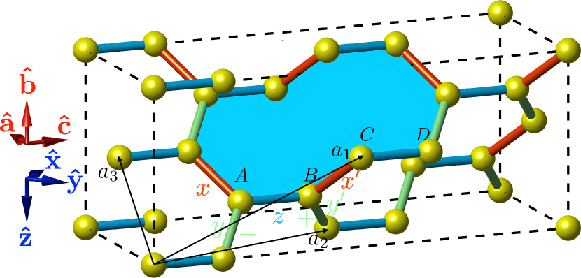
Figure 1: The sketch of the hyperhoneycomb lattice. The conventional orthorhombic unit cell is set by the crystallographic axes $\hat{{\bf a}},\hat{{\bf b}}$ and $\hat{{\bf c}}$. The three lattice vectors of the primitive face-centered orthorhombic lattice are given by $\mathbf{a}_{1}=\left(0,\sqrt{2},3\right)$, $\mathbf{a}_{2}=\left(1,0,3\right)$, $\mathbf{a}_{3}=\left(1,\sqrt{2},0\right)$ which is written in the crystallographic basis. The four sublattices $A,\,B,\,C$ and $D$ are shown, and we set $\mathbf{r}_{A}=\left(0,0,0\right)$. Different bond types $x$, $y$, and $z$ are marked by red, green, and blue, respectively. The Cartesian axes $\{\hat{{\bf x}},\hat{{\bf y}},\hat{{\bf z}}\}$ used to write the the spin Hamiltonian Eq. (2) is related to the crystallographic orthorhombic axes by $\hat{{\bf x}}=(\hat{{\bf a}}+\hat{{\bf c}})/\sqrt{2}$, $\hat{{\bf y}}=(\hat{{\bf c}}-\hat{{\bf a}})/\sqrt{2}$ and $\hat{{\bf z}}=-\hat{{\bf b}}$. The shaded region denotes a loop on the hyperhoneycomb lattice containing 10 sites.

II The spin-phonon model

In this section, we introduce the spin-phonon coupled Kitaev model on the hyperhoneycomb lattice and discuss its phonon dynamics. It is described by the following Hamiltonian:

$$\mathcal{H}=\mathcal{H}^{s}+\mathcal{H}^{\mathrm{ph}}+\mathcal{H}^{\text{c}}.$$ (1)

The first term in Eq. (1) is the spin Hamiltonian. The second term is the bare Hamiltonian for the acoustic phonons. The third term is the magnetoelastic coupling.

II.1 The Kitaev model on the hyperhoneycomb lattice

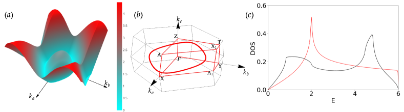
Figure 2: (a) The dispersion of the lowest branch of the fermionic excitations in the hyperhoneycomb Kitaev model through the plane of the nodal line ${\bf K}_{0}=(k_{a},k_{b},0)$, whose position in the Brillouin zone is explicitly shown in panel (b).(c) One-fermion density of states (DOS) of the isotropic Kitaev models on the honeycomb (red line) and the hyperhoneycomb (black line) lattices. In each case, the density of states is normalized to unity.

We start by revisiting the main features of the Kitaev QSL realized on the hyperhoneycomb lattice previously discussed in Refs.Hermanns et al. (2015); Halász et al. (2017). The hyperhoneycomb lattice is a face-centered orthorhombic lattice with four sites per primitive unit cell. Apart from translational symmetry, the crystal structure is invariant under the $D_{2h}$ point group symmetry. The conventional orthorhombic unit cell is set by the crystallographic axes $\{\hat{{\bf a}},\hat{{\bf b}},\hat{{\bf c}}\}$, as shown in Fig. 1. The Cartesian axes $\{\hat{{\bf x}},\hat{{\bf y}},\hat{{\bf z}}\}$ used to write the spin vector field is expressed as $\hat{{\bf x}}=(\hat{{\bf a}}+\hat{{\bf c}})/\sqrt{2}$, $\hat{{\bf y}}=(\hat{{\bf c}}-\hat{{\bf a}})/\sqrt{2}$ and $\hat{{\bf z}}=-\hat{{\bf b}}$. Different bond types $x$, $y$, and $z$ are marked by red, green, and blue, respectively. Note, however, that there are two non-equivalent types of $x$ and $y$ bonds, and the hyperhoneycomb structure can be viewed as a stacking of two types of zigzag chains formed by $x,y$ bonds and $x^{\prime},y^{\prime}$ bonds, each pair running along ${\bf a}\!+\!{\bf b}$ and ${\bf a}\!-\!{\bf b}$ directions, respectively. The two types of chains are interconnected with vertical $z$-bonds. Thus, in total, there are five types of nearest neighboring bonds: $x,x^{\prime},y,y^{\prime},$ and $z$.

The Kitaev spin model on the hyperhoneycomb lattice reads

$${\mathcal{H}}^{s}\!=\!-J\!\left(\!\sum_{\left\langle\mathbf{r}\mathbf{r}^{\prime}\right\rangle\in\{x,x^{\prime}\}}\!\!\!\!\!\sigma_{\mathbf{r}}^{x}\sigma_{\mathbf{r}^{\prime}}^{x}+\!\!\!\!\!\sum_{\left\langle\mathbf{r}\mathbf{r}^{\prime}\right\rangle\in\{y,y^{\prime}\}}\!\!\!\!\!\sigma_{\mathbf{r}}^{y}\sigma_{\mathbf{r}^{\prime}}^{y}+\!\!\!\!\!\sum_{\left\langle\mathbf{r}\mathbf{r}^{\prime}\right\rangle\in\{z\}}\!\!\!\!\!\sigma_{\mathbf{r}}^{z}\sigma_{\mathbf{r}^{\prime}}^{z}\right),$$ (2)

where $\mathbf{r}$ and $\mathbf{r}^{\prime}$ are sites on the three-dimensional hyperhoneycomb lattice, which we sketch in Fig.1 and the summation is done over five types of bonds. We also assumed the isotropic case with $J_{x}\!\!=\!\!J_{y}\!\!=\!\!J_{z}\!\!=\!\!J$. The symmetry of the Hamiltonian (2) involves a combined lattice and spin transformations You et al. (2012) [for detailed mathematical description, see Ref. Feng (2022); Feng et al. (2022)]. The results of the three $\pi$-rotations around the crystallographic axes ${\bf a}$, ${\bf b}$, and ${\bf c}$ are the following. Under $C_{2\bf a}$ rotation spins transform as $[\sigma^{x},\sigma^{y},\sigma^{z}]\rightarrow[-\sigma^{y},-\sigma^{x},-\sigma^{z}]$, under $C_{2\bf b}$ rotation $[\sigma^{x},\sigma^{y},\sigma^{z}]\rightarrow[-\sigma^{x},-\sigma^{y},\sigma^{z}]$, and under $C_{2\bf c}$ rotation $[\sigma^{x},\sigma^{y},\sigma^{z}]\rightarrow[\sigma^{y},\sigma^{x},-\sigma^{z}]$. Additionally, $D_{2h}$ group also contains the space inversion $I$ at the middle of $x,x^{\prime},y,y^{\prime}$ bonds, which together with spin transformation leads to $[\sigma^{x},\sigma^{y},\sigma^{z}]\rightarrow[\sigma^{y},\sigma^{x},\sigma^{z}]$. The transformation $C_{2\bf c}$, $C_{2\bf b}$ and $I$ constitute the canonical generators that generate the whole $D_{2h}$ group.

The exact solution of model (2) is based on the macroscopic number of local symmetries in the products of particular components of the spin operators around every plaquette $P$, which on the hyperhoneycomb lattice consists of ten sites (see shaded region in Fig.1) and is defined by the following plaquette operator $\hat{W}_{p}=\prod_{\mathbf{r}\in P}\sigma_{\mathbf{r}}^{\alpha(\mathbf{r})}$, where the spin component $\alpha(\mathbf{r})$ is given by the label of the outgoing bond direction. Since all plaquette operators $\hat{W}_{p}$ commute with the Hamiltonian, $[\hat{W}_{p},\mathcal{H}_{s}]=0$, and take eigenvalues of $\pm 1$, the Hilbert space of the spin Hamiltonian $\mathcal{H}_{s}$ can be divided into eigenspaces of $\hat{W}_{p}$. The ground state of the Kitaev model on the hyperhoneycomb lattice is the zero-flux state with all $\hat{W}_{p}=1$ Mandal and Surendran (2009); Hermanns et al. (2015). This, however, can not be derived exactly from the Lieb’s theorem Lieb (1994) but is only based on the numerical calculations Hermanns et al. (2015); Eschmann et al. (2020). Thus, strictly speaking, the Kitaev model on hyperhoneycomb lattice is not exactly solvable. Another striking difference between the hyperhoneycomb Kitaev spin liquid and its two-dimensional counterpart regards the effect of the thermal fluctuations on the stability of the ground-state zero-flux state. While in two-dimensional honeycomb lattice thermal fluctuations immediately destroy the zero-flux order of the $Z_{2}$ gauge field Nasu et al. (2014a); Feng et al. (2020), in three spatial dimensions there is a finite-temperature transition separating it from a high-temperature disordered flux state Nasu et al. (2014b); Yoshitake et al. (2017); Eschmann et al. (2020).

Using the Kitaev’s representation of spins in terms of Majorana fermions Kitaev (2006), $\sigma_{\mathbf{r}}^{\gamma}=ib_{\mathbf{r}}^{\gamma}c_{\mathbf{r}}^{\phantom{\gamma}}$ with $\gamma=x,y,z$ Kitaev (2006), the spin Hamiltonian Eq.(2) can be rewritten as

$$\mathcal{H}^{s}=\sum_{\gamma}\sum_{\langle\mathbf{r},\mathbf{r}^{\prime}\rangle_{\gamma}}iJ_{\gamma}^{\phantom{\gamma}}\eta_{\mathbf{r},\mathbf{r}^{\prime}}^{\gamma}c_{\mathbf{r}}^{\phantom{\gamma}}c_{\mathbf{r}^{\prime}}^{\phantom{\gamma}}=\frac{1}{2}\sum_{\mathbf{r},\mathbf{r}^{\prime}}\mathcal{H}_{\mathbf{r},\mathbf{r}^{\prime}}c_{\mathbf{r}}c_{\mathbf{r}^{\prime}},$$ (3)

where $\eta_{\mathbf{r},\mathbf{r}^{\prime}}^{\gamma}\equiv ib_{\mathbf{r}}^{\gamma}b_{\mathbf{r}^{\prime}}^{\gamma}=\pm 1$, $\mathcal{H}_{\mathbf{r},\mathbf{r}^{\prime}}=iJ_{\gamma}^{\phantom{\gamma}}\eta_{\mathbf{r},\mathbf{r}^{\prime}}^{\gamma}$ if $\mathbf{r}$ and $\mathbf{r}^{\prime}$ are neighboring sites connected by a $\gamma$ bond and $\mathcal{H}_{\mathbf{r},\mathbf{r}^{\prime}}=0$ otherwise. In the ground-state flux sector, we choose the gauge sector with all $\eta_{\mathbf{r},\mathbf{r}^{\prime}}^{\gamma}=1$, which corresponds to all $\hat{W}_{p}=1$. The quadratic fermionic Hamiltonian in Eq. (3) can be diagonalized via a standard procedure Kitaev (2006). Since the hyperhoneycomb lattice has four sites per unit cell, the resulting band structure has four fermion bands, $\xi=1\sim 4$ ($\xi=1,2$ are the two positive bands). The diagonal form of the Hamiltonian Halász et al. (2017)

$${\mathcal{H}}^{s}=\sum_{\mathbf{k}}\sum_{\xi=1}^{4}\varepsilon_{\mathbf{k},\xi}^{\phantom{{\dagger}}}[\psi_{\mathbf{k},\xi}^{{\dagger}}\psi_{\mathbf{k},\xi}^{\phantom{{\dagger}}}-1/2]$$ (4)

is then obtained by the unitary transformation $\tilde{\mathcal{H}}_{\mathbf{k}}^{\phantom{{\dagger}}}=\mathcal{W}_{\mathbf{k}}^{\phantom{{\dagger}}}\cdot\mathcal{E}_{\mathbf{k}}^{\phantom{{\dagger}}}\cdot\mathcal{W}_{\mathbf{k}}^{{\dagger}}$ of the Hermitian matrix $\tilde{\mathcal{H}}_{\mathbf{k}}^{\phantom{{\dagger}}}$ with elements $(\tilde{\mathcal{H}}_{\mathbf{k}})_{\nu\nu^{\prime}}=\frac{1}{N}\sum_{\mathbf{r}\in\nu}\sum_{\mathbf{r}^{\prime}\in\nu^{\prime}}\mathcal{H}_{\mathbf{r},\mathbf{r}^{\prime}}\,e^{i\mathbf{k}\cdot(\mathbf{r}^{\prime}-\mathbf{r})}$, where $\nu$ and $\nu^{\prime}$ denote sublattices $a,b,c,d$ shown in Fig. 1, and $\varepsilon_{\mathbf{k},\xi}=(\mathcal{E}_{\mathbf{k}})_{\xi\xi}$ are the fermionic energies. The fermionic eigenmodes are given by

$$\psi_{\mathbf{k},\xi}^{\phantom{{\dagger}}}=\frac{1}{\sqrt{2N}}\sum_{\nu=1}^{n}\left(\mathcal{W}_{\mathbf{k}}^{{\dagger}}\right)_{\xi\nu}\sum_{\mathbf{r}\in\nu}c_{\mathbf{r}}^{\phantom{{\dagger}}}\,e^{-i\mathbf{k}\cdot\mathbf{r}}.$$ (5)

Note that only the fermions $\psi_{\mathbf{k},\xi}$ with energies $\varepsilon_{\mathbf{k},\xi}>0$ are physical due to the particle-hole redundancy $\tilde{\mathcal{H}}_{-\mathbf{k}}^{\phantom{{\dagger}}}=-\tilde{\mathcal{H}}_{\mathbf{k}}^{*}$, which implies $\psi_{-\mathbf{k},\xi}^{\phantom{{\dagger}}}=\psi_{\mathbf{k},\xi}^{{\dagger}}$ and $\varepsilon_{-\mathbf{k},\xi}^{\phantom{{\dagger}}}=\varepsilon_{\mathbf{k},\xi}$. Thus, only two branches have positive spectrum. The lowest branch $\varepsilon_{\mathbf{k},1}$ [shown in Fig. 2 (a)] exhibits the nodal line on the $(k_{a},k_{b})$ plane [Fig. 2 (b)], which is protected by projective time-reversal symmetry Hermanns et al. (2015). By solving the equation $\varepsilon_{{\mathbf{k}},1}=0$, we obtained the functional form of the nodal line, ${\bf K}_{0}=(k_{a},k_{b},0)$, with

$$k_{b} =\frac{1}{\sqrt{2}}\arg\left(1-2\cos k_{a}\pm i\sqrt{1+4\cos k_{a}-2\cos 2k_{a}}\right).$$ (6)

The energy dispersion is linear if expanded around the nodal line, i.e. each point of the nodal line represents a Dirac cone. Importantly, the Fermi velocity varies along the nodal line and depends on the direction of the deviation from it, i.e. $v_{F}=v_{F}({\bf K}_{0},\delta{\bf k})$, where $\delta{\bf k}=(\delta k_{a},\delta k_{b},\delta k_{c})$. As we will see later, the spacial dependence of the Fermi velocity of the low-energy Majorana fermions will lead to the qualitative difference in the temperature dependence of the sound attenuation coefficient between the hyperhoneycomb model and the honeycomb Kitaev model Ye et al. (2020); Feng et al. (2021).

To further characterized the spectrum of Majorana fermions, in Fig. 2(c) we plot the density of states $\text{DOS}(E)=\sum_{\xi=1,2}\int_{BZ}\delta(E-\varepsilon_{{\bf k},\xi})d^{3}{\bf k}$ for the hyperhoneycomb Kitaev model (shown by the black line) where the contributions from both branches of Majorana fermions are summed up. The low-energy DOS is linear in energy, which follows directly from the linear low-energy dispersion and the dimension of the Fermi surface Perreault et al. (2015). For comparison, in Fig. 2(c) we also plot the DOS for the honeycomb model (shown by the red line). The differences between the DOS for these two lattices can be understood in terms of the number of fermionic bands, one for the honeycomb lattice and two for the hyperhoneycomb lattices, and their nodal structure - two Dirac points for the honeycomb lattice and the closed line of Dirac points for the hyperhoneycomb lattice. The former leads to the absence of the Van-Hove singularities and overall more flatten DOS for the hyperhoneycomb lattice. The latter is responsible for a faster growth of the hyperhoneycomb DOS at low energies, which is consistent with higher dimensionality of the nodal line and enlarged number of low-energy states.

II.2 Acoustic phonons on the hyperhoneycomb lattice

Next we find the spectrum of the acoustic phonons on the hyperhoneycomb lattice. The bare Hamiltonian for the acoustic phonons contains the kinetic and elastic energy, $\mathcal{H}^{\mathrm{ph}}=\mathcal{H}_{kinetic}^{\mathrm{ph}}+\mathcal{H}_{elastic}^{\mathrm{ph}}$, where $\mathcal{H}_{kinetic}^{\mathrm{ph}}=\sum_{{\bf q},\mu}\frac{\bf{P}_{-\bf q,\mu}\cdot\bf{P}_{\bf q,\mu}}{2\rho\delta_{V}}$ with $\bf{P}_{{\bf q},\mu}$ denoting the momentum of the phonon with polarization $\mu$, $\delta_{V}$ is the area enclosed in one unit cell and $\rho$ is the mass density of the lattice ions. The elastic contribution $\mathcal{H}_{elastic}^{\mathrm{ph}}$ can be expressed in terms of the strain tensor $\epsilon_{ij}=\frac{1}{2}\left(\partial_{i}u_{j}+\partial_{j}u_{i}\right)$, where ${\bf u}=\{u_{a},u_{b},u_{c}\}$ describes the displacement of an atom from its original location.

In order to describe the dynamics of the low-energy acoustic phonons, it is convenient to move away from the Hamiltonian formulation and employ instead the long-wavelength effective action $\mathcal{S}$ approach. To lowest order, it reads Landau, L. D. and Pitaevskii, L. P. and Kosevich, A. M. and Lifshitz, E. M. (2012)

$$\mathcal{S}_{\mathrm{ph}}^{(s)} =\int\mathrm{d}^{2}x\mathrm{d}\tau\,[\rho\,(\partial_{\tau}{\bf u})^{2}+F],\,\,F=\frac{1}{2}\mathcal{C}_{ijlk}\epsilon_{ij}\epsilon_{lk},$$ (7)

where $F$ is the elastic free energy and $C_{ijlk}$ denote the elements of the elastic modulus tensor. The number of independent non-zero $\mathcal{C}_{ijlk}$ is dictated by symmetry. The hyperhoneycomb lattice has Fddd space group, which is generated by three glide planes, which are passing through the bond center of either of $x,x^{\prime},y,y^{\prime}$ bonds and are orthogonal to the ${\bf a},\,{\bf b},\,{\bf c}$ axes, respectively. The hyperhoneycomb lattice also has inversion symmetry with respect to the bond center of $x,x^{\prime},y,y^{\prime}$ bonds. The inversion thus can be generated by the product of glide mirrors, e.g., the inversion on the $x$ bond can be generated by $d_{1}^{-1}d_{2}d_{3}^{-1}$, where each $d_{i}$ glide is accompanied by a half of lattice translation along the primitive lattice vector ${\bf a}_{i}$ Choi et al. (2019). Thus the point group is isomorphic to the $D_{2h}$, for which there are nine independent non-zero components of the elastic modulus tensor $C_{iiii},C_{ijij},C_{iijj}$, where $i$ and $j$ denote $a,b,c$. Performing the Fourier transform, ${\bf u}({\bf r})=\frac{1}{\sqrt{N}}\sum_{\bf q}e^{i{\bf q}\cdot{\bf r}}{\bf u}_{\bf q}$, the elastic free energy can be explicitly written as

$$F=\frac{1}{2}\begin{pmatrix}C_{aaaa}q_{a}^{2}+C_{acac}q_{c}^{2}+C_{abab}q_{b}^{2}&q_{b}q_{a}\,(C_{aabb}+C_{abab})&q_{a}q_{c}\,(C_{aacc}+C_{acac})\\ q_{b}q_{a}(C_{aabb}+C_{abab})&C_{abab}q_{a}^{2}+C_{bcbc}q_{c}^{2}+C_{bbbb}q_{b}^{2}&q_{b}q_{c}\,(C_{bbcc}+C_{bcbc})\\ q_{a}q_{c}\,(C_{aacc}+C_{acac})&q_{b}q_{c}\,(C_{bbcc}+C_{bcbc})&C_{acac}q_{a}^{2}+C_{cccc}q_{c}^{2}+C_{bcbc}q_{b}^{2}\end{pmatrix},$$ (8)

where $q_{a}=q\sin\theta_{\mathbf{q}}\cos\phi_{\mathbf{q}}$, $q_{b}=q\sin\theta_{\mathbf{q}}\sin\phi_{\mathbf{q}}$ and $q_{c}=q\cos\theta_{\mathbf{q}}$ are the components of the acoustic vector ${\bf q}$ in the orthorhombic reference frame. By diagonalizing the matrix (8), we compute eigenmodes, one longitudinal and two transverse acoustic modes, and the corresponding eigenenergies: the longitudinal and transverse acoustic phonons are then given by

$$\left(\begin{array}[]{c}u_{{\bf q},a}\\ u_{{\bf q},b}\\ u_{{\bf q},c}\end{array}\right)=\begin{pmatrix}R_{11}&R_{12}&R_{13}\\ R_{21}&R_{22}&R_{23}\\ R_{31}&R_{32}&R_{33}\end{pmatrix}\left(\begin{array}[]{c}{\tilde{u}}_{{\bf q}}^{\parallel}\\ {\tilde{u}}_{{\bf q}}^{\perp_{1}}\\ {\tilde{u}}_{{\bf q}}^{\perp_{2}}\end{array}\right),$$ (9)

where $\hat{R}\equiv\hat{R}(\theta_{\mathbf{q}},\phi_{\mathbf{q}})$ is the transformation matrix, ${\tilde{u}}_{{\bf q}}^{\parallel}$, ${\tilde{u}}_{{\bf q}}^{\perp_{1}}$ and ${\tilde{u}}_{{\bf q}}^{\perp_{2}}$ are the longitudinal and transverse acoustic eigenmodes, respectively. The energies of the longitudinal and transverse acoustic phonons are

$$\Omega^{\nu}_{\bf q}=v_{s}^{\nu}(\theta_{\mathbf{q}},\phi_{\mathbf{q}})q,$$ (10)

where the sound velocities $v_{s}^{\nu}$ for the longitudinal acoustic mode, $v_{s}^{\parallel}(\theta_{\mathbf{q}},\phi_{\mathbf{q}})$, and two transverse modes, $v_{s}^{\perp_{1}}(\theta_{\mathbf{q}},\phi_{\mathbf{q}})$ and $v_{s}^{\perp_{2}}(\theta_{\mathbf{q}},\phi_{\mathbf{q}})$ are anisotropic in space.

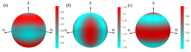
Figure 3: Angular dependence of the sound velocities [in the unit of $10^{4}$ m/s] for (a) longitudinal mode ($v_{s}^{\parallel}(\theta,\phi)$) and (b) in-plane transverse mode ($v_{s}^{\perp_{1}}(\theta,\phi)$) and (c) out-of-plane transverse mode ($v_{s}^{\perp_{2}}(\theta,\phi)$) computed, for the elastic modulus coefficients close to those computed for $\beta$-Li₂IrO₃ Tsi .

In Fig. 3, we plot the angular dependence of these velocities computed for the elastic modulus tensor coefficients close to those computed for $\beta$-Li₂IrO₃: we set $C_{iiii}=2800$ kbar, $i=a,b,c$, $C_{aacc}=C_{bbcc}=1300$ kbar, $C_{aabb}=C_{abab}=C_{acac}=C_{bcbc}=900$ kbar Tsi . We see that the angular dependence of the sound velocities is not that strong. In the plot, the maximum sound velocity is estimated to be $2\times 10^{4}$m/s, which is in the middle of the sound velocities reported for different directions in $\alpha$-RuCl₃ Lebert et al. (2022). For the elastic modulus tensor given above, and restricting phonon modes to $ab$, $bc$ and $ac$ crystallographic planes, we numerically checked that the first column of the rotation matrix $\hat{R}$ corresponding to the longitudinal mode indeed gives the vector parallel to $\mathbf{q}$, i.e. $\left(R_{11},R_{21},R_{31}\right)^{\mkern-1.5mu\mathsf{T}}=\left(\sin\theta_{\mathbf{q}}\cos\phi_{\mathbf{q}},\sin\theta_{\mathbf{q}}\sin\phi_{\mathbf{q}},\cos\theta_{\mathbf{q}}\right)^{\mkern-1.5mu\mathsf{T}}$, while the second and the third columns are perpendicular to $\mathbf{q}$ (the second column with label $\perp_{1}$ corresponds to the in-plane transverse mode, and the third column with label $\perp_{2}$ corresponds to the out-of-plane transverse mode).

Knowing the acoustic phonon dispersion relations (10), we can now determine the free phonon propagator in terms of lattice displacement field $\tilde{u}_{{\bf q}}^{\nu}$ as

$$D_{{\bf q}}^{(0)\,\nu\nu^{\prime}}(t)=-i\langle{\mathcal{T}}\tilde{u}_{-{\bf q}}^{\nu}(t)\tilde{u}_{{\bf q}}^{\nu^{\prime}}(0)\rangle^{(0)},$$ (11)

where ${\mathcal{T}}$ is time ordering operator, the superscript $(0)$ denotes the bare propagator, $\nu=\parallel,\perp_{1},\perp_{2}$ labels the polarization, and $\tilde{u}_{{\bf q}}^{\nu}$ are phonon eigenmodes in the corresponding polarization, which in the second quantized form can be written as

$$\tilde{u}_{{\bf q}}^{\nu}(t)=i\left(\frac{\hbar}{2\rho\,\delta_{V}\Omega^{\nu}_{\bf q}}\right)^{1/2}({\tilde{a}}_{\bf q}e^{-i\Omega^{\nu}_{\bf q}t}+{\tilde{a}}^{\dagger}_{-{\bf q}}e^{i\Omega^{\nu}_{\bf q}t}),$$ (12)

where $\delta_{V}$ is the area enclosed in one unit cell and $\rho$ is the mass density of the lattice ions. In the momentum and frequency space, the bare phonon propagator is then given by

$$D^{(0)\nu\nu}({\bf q},\Omega)=-\frac{\hbar}{\rho\,\delta_{V}}\frac{1}{\Omega^{2}-(\Omega^{\nu}_{\bf q})^{2}+i0^{+}}.$$ (13)

The dynamics of phonons will be thus described by the decay and scattering of these eigenmodes on low-energy fractionalized excitations of the Kitaev model, which can be accounted for by the phonon self-energy $\Pi_{\mathrm{ph}}({\bf q},\Omega)$ Ye et al. (2020), which for this case we will discuss later in Sec. III. The renormalized phonon propagator is then given by the Dyson equation $D({\bf q},\Omega)=\left[\left(D^{(0)}({\bf q},\Omega)\right)^{-1}-\Pi_{\mathrm{ph}}({\bf q},\Omega)\right]^{-1}$.

II.3 The Majorana fermion-phonon coupling vertices

In order to study the phonon dynamics in the Kitaev spin liquid, it remains to compute the Majorana fermion-phonon (MFPh) coupling vertices, which we will do in this section. We recall that the magneto-elastic coupling $\mathcal{H}^{\text{c}}$ arises from the change in the Kitaev coupling due to the lattice vibrations. In the long wavelength limit for acoustic phonons, the coupling Hamiltonian on the bond can be written in a differential form as

$$\mathcal{H}^{\text{c}}_{{\bf r},{\bf r}+{\bf M}_{\alpha}}=\lambda{\bf M}_{\alpha}\cdot\left[\left({\bf M}_{\alpha}\cdot{\bf\nabla}\right){\bf u}({\bf r})\right]\sigma_{\bf r}^{\alpha}\sigma_{{\bf r}+{\bf M}_{\alpha}}^{\alpha},$$ (14)

where $\lambda\sim\left(\frac{\mathrm{d}J}{\mathrm{d}{r}}\right)_{\textmd{e q}}\ell_{a}$ is the strength of the spin-phonon interaction and $\ell_{a}$ is the lattice constant, and ${\bf M}_{\alpha}={\bf M}_{1},...{\bf M}_{5}$ are five nearest neighboring vectors corresponding, respectively, to $y,y^{\prime},x,x^{\prime},z$ bonds shown in Fig.4. Using these vectors, we can write the spin-phonon coupling Hamiltonian explicitly:

$$\mathcal{H}^{\text{c}}= \frac{1}{4}\lambda\sum_{{\bf r}_{A}}\bigg{(}4\sigma_{{\bf r}_{A}}^{z}\sigma_{{\bf r}_{A}+{\bf M}_{5}}^{z}\epsilon_{cc}+\sigma_{{\bf r}_{A}}^{y}\sigma_{{\bf r}_{A}+{\bf M}_{2}}^{y}(\epsilon_{aa}+2\epsilon_{bb}+\epsilon_{cc}-2\sqrt{2}(\epsilon_{ab}-\epsilon_{bc})-2\epsilon_{ac})$$

$$+\sigma_{{\bf r}_{A}}^{x}\sigma_{{\bf r}_{a}+{\bf M}_{4}}^{x}(\epsilon_{aa}+2\epsilon_{bb}+\epsilon_{cc}-2\sqrt{2}(\epsilon_{ab}+\epsilon_{bc})+2\epsilon_{ac})\bigg{)}$$ (15)

$$+\sum_{{\bf r}_{B}}\bigg{(}\sigma_{{\bf r}_{B}}^{y}\sigma_{{\bf r}_{B}+{\bf M}_{1}}^{y}(\epsilon_{aa}+2\epsilon_{bb}+\epsilon_{cc}+2\sqrt{2}(\epsilon_{ab}-\epsilon_{bc})-2\epsilon_{ac})+\sigma_{{\bf r}_{B}}^{x}\sigma_{{\bf r}_{B}+{\bf M}_{3}}^{x}(\epsilon_{aa}+2\epsilon_{bb}+\epsilon_{cc}+2\sqrt{2}(\epsilon_{ab}+\epsilon_{bc})+2\epsilon_{ac})\bigg{)},$$

where we use a short notation $\epsilon_{ij}\equiv\epsilon_{ij}({\bf r})$ with ${\bf r}={\bf r}_{A}$ or ${\bf r}_{B}$ depending on the bond and $i,j$ one of the orthorhombic directions $a,b,c$.

Under the D_2h point group symmetry, the spin-phonon Hamiltonian has four independent symmetry channels, $A_{g}$, $B_{1g}$, $B_{2g}$, and $B_{3g}$, which are inversion-symmetric irreducible representations (IRRs) of this group. The linear combinations of the strain tensors that transform as the D_2h are $\epsilon_{aa}$, $\epsilon_{bb}$, and $\epsilon_{cc}$, in the $A_{g}$ channel, and $\epsilon_{ab}$, $\epsilon_{ac}$ and $\epsilon_{bc}$ in $B_{1g}$, $B_{2g}$, and $B_{3g}$, respectively. By writing the linear combinations of the Kitaev interactions that transform according to these IRRs, we express the spin-phonon coupling Hamiltonian Eq. (II.3) as a sum of four independent contributions, ${\mathcal{H}}^{c}=\mathcal{H}^{c}_{A_{g}}+\mathcal{H}^{c}_{B_{1g}}+\mathcal{H}^{c}_{B_{2g}}+\mathcal{H}^{c}_{B_{3g}}$ with

$$\mathcal{H}^{c}_{A_{g}} =\lambda_{A_{g}}\sum_{{\bf r}_{A},{\bf r}_{B}}\left[4\epsilon_{cc}\sigma_{{\bf r}_{A}}^{z}\sigma_{{\bf r}_{A}+{\bf M}_{5}}^{z}+(\epsilon_{aa}+2\epsilon_{bb}+\epsilon_{cc})(\sigma_{{\bf r}_{B}}^{y}\sigma_{{\bf r}_{B}+{\bf M}_{1}}^{y}+\sigma_{{\bf r}_{A}}^{y}\sigma_{{\bf r}_{A}+{\bf M}_{2}}^{y}+\sigma_{{\bf r}_{B}}^{x}\sigma_{{\bf r}_{B}+{\bf M}_{3}}^{x}+\sigma_{{\bf r}_{A}}^{x}\sigma_{{\bf r}_{A}+{\bf M}_{4}}^{x})\right],$$

$$\mathcal{H}^{c}_{B_{1g}} =\lambda_{B_{1g}}\sum_{{\bf r}_{A},{\bf r}_{B}}\epsilon_{ab}(\sigma_{{\bf r}_{B}}^{y}\sigma_{{\bf r}_{B}+{\bf M}_{1}}^{y}-\sigma_{{\bf r}_{A}}^{y}\sigma_{{\bf r}_{A}+{\bf M}_{2}}^{y}+\sigma_{{\bf r}_{B}}^{x}\sigma_{{\bf r}_{B}+{\bf M}_{3}}^{x}-\sigma_{{\bf r}_{A}}^{x}\sigma_{{\bf r}_{A}+{\bf M}_{4}}^{x}),$$

$$\mathcal{H}^{c}_{B_{2g}} =\lambda_{B_{2g}}\sum_{{\bf r}_{A},{\bf r}_{B}}\epsilon_{ac}(-\sigma_{{\bf r}_{B}}^{y}\sigma_{{\bf r}_{B}+{\bf M}_{1}}^{y}-\sigma_{{\bf r}_{A}}^{y}\sigma_{{\bf r}_{A}+{\bf M}_{2}}^{y}+\sigma_{{\bf r}_{B}}^{x}\sigma_{{\bf r}_{B}+{\bf M}_{3}}^{x}+\sigma_{{\bf r}_{A}}^{x}\sigma_{{\bf r}_{A}+{\bf M}_{4}}^{x}),$$ (16)

$$\mathcal{H}^{c}_{B_{3g}} =\lambda_{B_{3g}}\sum_{{\bf r}_{A},{\bf r}_{B}}\epsilon_{bc}(-\sigma_{{\bf r}_{B}}^{y}\sigma_{{\bf r}_{B}+{\bf M}_{1}}^{y}+\sigma_{{\bf r}_{A}}^{y}\sigma_{{\bf r}_{A}+{\bf M}_{2}}^{y}+\sigma_{{\bf r}_{B}}^{x}\sigma_{{\bf r}_{B}+{\bf M}_{3}}^{x}-\sigma_{{\bf r}_{A}}^{x}\sigma_{{\bf r}_{A}+{\bf M}_{4}}^{x}),$$

where we absorbed numerical prefactors into the definitions of the coupling constants $\lambda_{A_{g}},\lambda_{B_{1g}},\lambda_{B_{2g}}$ and $\lambda_{B_{3g}}$.

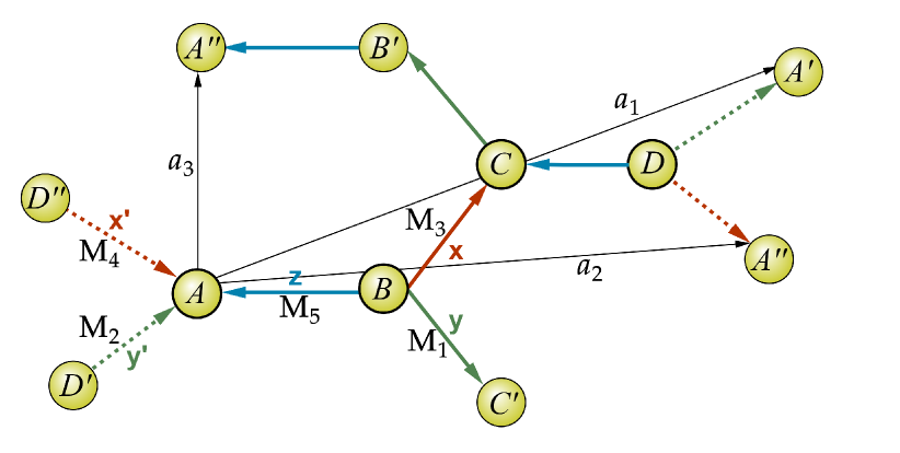
Figure 4: $A,B,C,D$ denote four sublattices of the hyperhoneycomb lattice. ${\bf M}_{1}=\frac{1}{2}(1,\sqrt{2},-1)$, ${\bf M}_{2}=\frac{1}{2}(1,-\sqrt{2},-1)$, ${\bf M}_{3}=\frac{1}{2}(-1,-\sqrt{2},-1)$, ${\bf M}_{4}=\frac{1}{2}(-1,\sqrt{2},-1)$ and ${\bf M}_{5}=(0,0,1)$ are five nearest neighboring vectors, corresponding to $y,y^{\prime},x,x^{\prime},z$ bonds, respectively (all the vectors are given in the crystallographic axes $\hat{{\bf a}},\hat{{\bf b}}$ and $\hat{{\bf c}}$). We use the following convention: an arrow pointing from site $\mathbf{r}$ to $\mathbf{r}^{\prime}$ means $u_{\mathbf{r},\mathbf{r}^{\prime}}$ on the corresponding bond is positive.

Next,we express the spin operators in terms of the Majorana fermions and assume the ground state flux sector. Then we perform the Fourier transformation on both the strain tensor, $\epsilon_{ij}({\bf r})=\frac{1}{\sqrt{N}}\sum_{\bf q}\frac{i}{2}\left(q_{i}u_{{\bf q},j}+q_{j}u_{{\bf q},i}\right)e^{i\mathbf{q}\cdot\mathbf{r}}$, and the Majorana fermions, $c_{{\bf r},\alpha}=\sqrt{\frac{2}{N}}\sum_{\bf k}c_{{\bf k},\alpha}e^{i\bf{k}\cdot\bf{r}_{\alpha}}$, where $\alpha=A,\,B,\,C,\,D$ is the sublattice label [see Fig. 4]. Now the products of the spin variables on all non-equivalent bonds can be written as (with the long wavelength approximation $\mathbf{q}\to 0$ applied):

$$\sigma_{\bf{r}}^{y}\sigma_{\bf{r+M_{1}}}^{y}\to{\bf A}^{\mkern-1.5mu\mathsf{T}}_{\bf{-q-k}}S_{\bf{k}}^{\dagger}\begin{pmatrix}0&-ie^{i\bf{k\cdot a_{3}}}&0&0\\ ie^{-i\bf{k\cdot a_{3}}}&0&0&0\\ 0&0&0&0\\ 0&0&0&0\end{pmatrix}S_{\bf{k}}\bf{A_{\bf{k}}},$$

$$\sigma_{\bf{r}}^{y}\sigma_{\bf{r+M_{2}}}^{y}\to{\bf A}^{\mkern-1.5mu\mathsf{T}}_{\bf{-q-k}}S_{\bf{k}}^{\dagger}\begin{pmatrix}0&0&0&0\\ 0&0&0&0\\ 0&0&0&ie^{i\bf{k\cdot a_{1}}}\\ 0&0&-ie^{-i\bf{k\cdot a_{1}}}&0\end{pmatrix}S_{\bf{k}}\bf{A_{\bf{k}}},$$

$$\sigma_{\bf{r}}^{x}\sigma_{\bf{r+M_{3}}}^{x}\to{\bf A}^{\mkern-1.5mu\mathsf{T}}_{\bf{-q-k}}S_{\bf{k}}^{\dagger}\begin{pmatrix}0&-i&0&0\\ i&0&0&0\\ 0&0&0&0\\ 0&0&0&0\end{pmatrix}S_{\bf{k}}\bf{A_{\bf{k}}},$$

$$\sigma_{\bf{r}}^{x}\sigma_{\bf{r+M_{4}}}^{x}\to{\bf A}^{\mkern-1.5mu\mathsf{T}}_{\bf{-q-k}}S_{\bf{k}}^{\dagger}\begin{pmatrix}0&0&0&0\\ 0&0&0&0\\ 0&0&0&ie^{i\bf{k\cdot a_{2}}}\\ 0&0&-ie^{-i\bf{k\cdot a_{2}}}&0\end{pmatrix}S_{\bf{k}}\bf{A_{\bf{k}}},$$

$$\sigma_{\bf{r}}^{z}\sigma_{\bf{r+M_{5}}}^{z}\to{\bf A}^{\mkern-1.5mu\mathsf{T}}_{\bf{-q-k}}S_{\bf{k}}^{\dagger}\begin{pmatrix}0&0&-i&0\\ 0&0&0&i\\ i&0&0&0\\ 0&-i&0&0\end{pmatrix}S_{\bf{k}}\bf{A_{\bf{k}}},$$

where ${\bf a}_{i}$ are the primitive unit vectors, $S_{\bf{k}}={\rm diag}\{e^{i\bf{k}\cdot{\bf r}_{\alpha}}\}_{\alpha=C,B,D,A}$ is the diagonal matrix in the sublattice basis, and the vector ${\bf A}_{\bf{k}}=\left(c_{{\bf k},C},c_{{\bf k},B},c_{{\bf k},D},c_{{\bf k},A}\right)^{\mkern-1.5mu\mathsf{T}}$. The Majorana-phonon coupling Hamiltonian in the momentum space is now can be written as ${\mathcal{H}}^{c}=\sqrt{\frac{2}{N}}\sum_{{\bf q},{\bf k}}{\mathcal{H}}_{{\bf q},{\bf k}}$, where each contribution ${\mathcal{H}}_{{\bf q},{\bf k}}$ can be decomposed into the irreducible representations $A_{g},B_{1g},B_{2g}$ and $B_{3g}$ [see Appendix A for explicit expressions]. Note also that ${\bf A}_{\bf{k}}$ is written in this particular permuted basis of the Majorana fermions in order to use the convenience of the auxiliary Pauli matrices in the representation of the coupling Hamiltonians as shown in Eq. (A).

Next we express the phonon modes in terms of the transverse and longitudinal eigenmodes defined in Eq. (9). Then ${\mathcal{H}}_{{\bf q},{\bf k}}$ terms in the corresponding polarizations are given by

$${\mathcal{H}}^{\parallel}_{{\bf q},\bf{k}} =\tilde{u}_{{\bf q}}^{\parallel}\,{\bf A}_{\bf{-q-k}}^{\mkern-1.5mu\mathsf{T}}\,S_{\bf{k}}^{\dagger}\,\hat{\lambda}_{{\bf q},{\bf k}}^{\parallel}\,S_{\bf{k}}\,{\bf A}_{\bf{k}}$$

$${\mathcal{H}}^{\perp_{1}}_{{\bf q},\bf{k}} =\tilde{u}_{{\bf q}}^{\perp_{1}}\,{\bf A}_{\bf{-q-k}}^{\mkern-1.5mu\mathsf{T}}\,S_{\bf{k}}^{\dagger}\,\hat{\lambda}_{{\bf q},{\bf k}}^{\perp_{1}}\,S_{\bf{k}}\,{\bf A}_{\bf{k}}$$ (17)

$${\mathcal{H}}^{\perp_{2}}_{{\bf q},\bf{k}} =\tilde{u}_{{\bf q}}^{\perp_{1}}\,{\bf A}_{\bf{-q-k}}^{\mkern-1.5mu\mathsf{T}}\,S_{\bf{k}}^{\dagger}\,\hat{\lambda}_{{\bf q},{\bf k}}^{\perp_{2}}\,S_{\bf k}\,{\bf A}_{\bf k}.$$

The explicit expressions for the MFPh coupling vertices for longitudinal and transverse phonon modes are given in Appendix A. Note also that since we are using the long wavelength limit for the phonons, we only kept the leading in $q$ terms in all $\hat{\lambda}_{{\bf q},{\bf k}}^{\nu}$.

III Phonon polarization bubble

At the lowest order, the phonon self-energy is given by the polarization bubble Ye et al. (2020)

$$\Pi_{\mathrm{ph}}^{\mu\nu}({\bf q},\Omega)=i\operatorname{Tr}{[\hat{\lambda}^{\mu}_{{\bf q},{\bf k}}\mathcal{G}({\bf k},\omega)\hat{\lambda}^{\nu}_{{\bf q},{\bf k}}\mathcal{G}({\bf k}-{\bf q},\omega+\Omega)]},$$ (18)

where $\hat{\lambda}^{{\mu}(\nu)}_{{\bf q},{\bf k}}$ are the MFPh coupling vertices for $\mu(\nu)=\parallel,\perp_{1},\perp_{2}$, and $\mathcal{G}({\bf k},\omega)$ denotes the Majorana fermions Green’s function for the lowest fermionic branch given by $\hat{\mathcal{G}}({\bf k},\omega)=-i\int_{-\infty}^{+\infty}\mathrm{d}t\langle{\mathcal{T}}\psi_{{\bf k},1}(t)\psi_{-{\bf k},1}^{\mkern-1.5mu\mathsf{T}}(0)\rangle e^{i\omega t}$ (in the following, we omit the branch index and simply write $\psi_{{\bf k}}\equiv\psi_{{\bf k},1}$).

Since we are interested in the phonon decay and scattering at finite temperature, it is convenient to use the Matsubara representation for the Majorana Green’s functions:

$$\Pi_{\mathrm{ph}}^{\mu\nu}\left(\mathbf{q},i\Omega_{n}\right)=\int_{\mathrm{BZ}}\mathrm{d}\mathbf{k}\operatorname{Tr}\left[\hat{\lambda}_{\mathbf{q},\mathbf{k}}^{\mu}\hat{\mathcal{G}}\left(\mathbf{k},i\omega_{m}+i\Omega_{n}\right)\hat{\lambda}_{\mathbf{q},\mathbf{k}}^{\nu}\hat{\mathcal{G}}\left(\mathbf{k}+\mathbf{q},i\omega_{m}\right)\right]$$

$$= \int_{\mathrm{BZ}}\mathrm{d}\mathbf{k}\operatorname{Tr}\left[\hat{\lambda}_{\mathbf{q},\mathbf{k}}^{\mu}\hat{\mathcal{W}}_{\mathbf{k}}^{\dagger}\hat{G}\left(\mathbf{k},i\omega_{m}+i\Omega_{n}\right)\hat{\mathcal{W}}_{\mathbf{k}}\hat{\lambda}_{\mathbf{q},\mathbf{k}}^{\nu}\hat{\mathcal{W}}_{\mathbf{k}+\mathbf{q}}^{\dagger}\hat{G}\left(\mathbf{k}+\mathbf{q},i\omega_{m}\right)\hat{\mathcal{W}}_{\mathbf{k}+\mathbf{q}}\right]$$ (19)

$$= \int_{\mathrm{BZ}}\mathrm{d}\mathbf{k}\sum_{ij}\sum_{l}\left[\left(\hat{\mathcal{W}}_{\mathbf{k}+\mathbf{q}}\hat{\lambda}_{\mathbf{q},\mathbf{k}}^{\mu}\hat{\mathcal{W}}_{\mathbf{k}}^{\dagger}\right)\hat{E}_{i}\left(\hat{\mathcal{W}}_{\mathbf{k}}\hat{\lambda}_{\mathbf{q},\mathbf{k}}^{\nu}\hat{\mathcal{W}}_{\mathbf{k}+\mathbf{q}}^{\dagger}\right)\hat{E}_{j}\right]_{ll}P_{\mathbf{k},ij}$$

where $\operatorname{Tr}[\ldots]$ in the first two lines sums over the Matsubara frequencies $i\omega_{m}$. $\hat{G}(\mathbf{k},\omega)=\left(\begin{array}[]{cc}g(\mathbf{k},\omega)&0\\ 0&\bar{g}(\mathbf{k},\omega)\end{array}\right)$ is the quasiparticle Green’s function, and

$$g(\mathbf{k},\omega)=-i\int\mathrm{d}t\left\langle{\mathcal{T}}\psi_{\mathbf{k}}(t)\psi_{\mathbf{k}}^{\dagger}(0)\right\rangle e^{i\omega t}=\frac{1}{\omega-\varepsilon_{\mathbf{k}}+i0^{+}}$$

$$\bar{g}(\mathbf{k},\omega)=-i\int\mathrm{d}t\left\langle{\mathcal{T}}\psi_{\mathbf{k}}^{\dagger}(t)\psi_{\mathbf{k}}(0)\right\rangle e^{i\omega t}=\frac{1}{\omega+\varepsilon_{\mathbf{k}}-i0^{+}}.$$ (20)

$\mathcal{W}_{\mathbf{k}}$ is the unitary matrix that diagonalizes the Majorana fermion Hamiltonian Halász et al. (2017). $\hat{E}_{i}=\left(\begin{array}[]{cc}\delta_{i1}&0\\ 0&\delta_{i2}\end{array}\right)$ serves to pick up a specific entry of a matrix. The summation over the Matsubara frequencies gives the dynamic part of the matrix entries

$$P_{\mathbf{k},ij}=T\sum_{i\omega_{m}}\left[\hat{G}\left(\mathbf{k},i\omega_{m}+i\Omega_{n}\right)_{ii}\hat{G}\left(\mathbf{k}+\mathbf{q},i\omega_{m}\right)_{jj}\right].$$ (21)

Their explicit expressions are given in Appendix C.

IV Angular dependence of the attenuation coefficient

In this section, we will compute the attenuation coefficient for the lossy acoustic wave function which decays with distance away from the driving source as

$${\bf u}({\bf x},t)={\bf u}_{0}e^{-\alpha_{s}({\bf q})x}e^{i(\Omega_{\mathbf{q}}t-{\bf q}\cdot{\bf x})}.$$ (22)

where ${{\bf u}}({\bf x},t)$ is the lattice displacement vector, ${\bf u}_{0}={{\bf u}}({\bf x}={{\bf 0}},t=0)$, $\Omega_{\mathbf{q}}$ is the acoustic wave frequency and ${\bf q}=q(\sin\theta_{\mathbf{q}}\cos\phi_{\mathbf{q}},\sin\theta_{\mathbf{q}}\sin\phi_{\mathbf{q}},\cos\theta_{\mathbf{q}})$ is the propagation vector. The attenuation coefficient $\alpha_{s}^{\mu}({\bf q})$ for a given phonon polarization $\mu=\parallel,\perp_{1},\perp_{2}$, defined as the inverse of the phonon mean free path, can be calculated from the diagonal component of the imaginary part of the phonon self-energy as Ye et al. (2020)

$$\alpha_{s}^{\mu}({\bf q})=-\frac{1}{2\rho\delta_{V}\left[v_{s}^{\mu}(\theta_{\mathbf{q}},\phi_{\mathbf{q}})\right]^{2}q}{\rm Im}\left.\Pi^{\mu\mu}_{\mathrm{ph}}({\bf q},\Omega)\right|_{\Omega=v_{s}^{\mu}(\theta_{\mathbf{q}},\phi_{\mathbf{q}})q}.$$ (23)

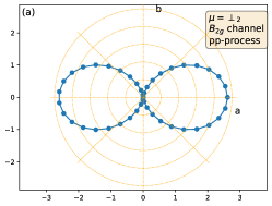
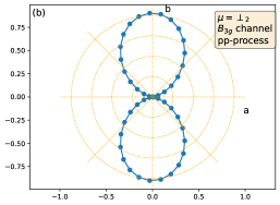
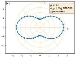
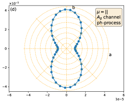
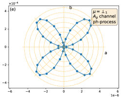
Figure 5: The angular dependence of sound attenuation coefficient $\alpha_{s}^{\mu}(\theta_{\mathbf{q}}\!=\!90^{\circ},\phi_{\mathbf{q}})$ in the $ab$-plane. The pp-processes contribute to the attenuation of the out-of-plane transverse phonon mode ($\alpha_{s}^{\perp_{2}}$) in (a) $B_{2g}$ channel, (b) $B_{3g}$ channel, and (c) combined $B_{2g}$ and $B_{3g}$ channels. The ph-processes contribute to (d) the attenuation of the longitudinal phonon ($\alpha_{s}^{\|}$) and to (e) the attenuation of the in-plane transverse phonon mode ($\alpha_{s}^{\perp_{1}}$) in the $A_{g}$ channel. The radius represents the magnitude of $\alpha_{s}^{\mu}$ in the units of $10^{-5}\rho\delta_{V}$. The calculation is performed at $T=0.02\,J$.

IV.1 Kinematic constraints and the estimates for the sound and Fermi velocities in $\beta$-Li₂IrO₃

Before analyzing the angular dependence of the sound attenuation coefficient, we need first discuss the kinematic constraints determining type of the processes involved in sound attenuation. In the zero-flux low temperature phase, both momentum and energy are conserved and kinematic constrains are primarily determined by the relative strength of acoustic phonon velocity $v_{s}(\theta_{\mathbf{q}},\phi_{\mathbf{q}})$ and Fermi velocity $v_{F}({\bf K_{0}},\theta_{\delta\mathbf{k}},\phi_{\delta_{\mathbf{k}}})$ (the slope of the Dirac cone at each point of the nodal line), which in the most general case are both angular dependent. These constraints determine whether the decay of the acoustic phonon happens in the particle- hole (ph-) or in the particle-particle (pp-) channel. Here, by particle and hole, we mean if the state of the Majorana fermion at $\varepsilon_{\mathbf{k}}$ ($\varepsilon_{\mathbf{k}}=\varepsilon_{\mathbf{k},1}$) is occupied or empty. In other words, the particle number refers to that of the complex fermion $\psi_{\mathbf{k}}$ ($\psi_{\mathbf{k}}=\psi_{\mathbf{k},1}$) in Eq.(4).

Here we assume that the angular dependence of $v_{s}(\theta_{\mathbf{q}},\phi_{\mathbf{q}})$ in $\beta$-Li₂IrO₃ is weak [see the magnitude scale bars in Fig. 3] and consider it to be equal to $v_{s}$. However, the Fermi velocity $v_{F}({\bf K_{0}},\theta_{\delta\mathbf{k}},\phi_{\delta\mathbf{k}})$ varies strongly between $v_{F}=0$ along the nodal line and $\max(v_{F})$, which can be estimated from the magnitude of the Kitaev coupling, which in $\beta$-Li₂IrO₃ is $J\simeq 20\,meV$ Ruiz et al. (2021); Yang et al. ; Halloran et al. . Taking the lattice constant to be equal to $\ell=0.23\,nm$ Villars and Cenzual , we estimate $\max(v_{F})=3\,J\ell=2.1\times 10^{4}\,m/s$. According to the estimation of the sound velocity in Sec. II.2, $v_{s}^{\|}\simeq 2.0\times 10^{4}m/s\lessapprox\max(v_{F})$, and $v_{s}^{\perp_{1,2}}\simeq 1.1\times 10^{4}m/s<\max(v_{F})$. When $v_{s}<\max(v_{F})$, the ph-processes are allowed but since they require finite occupation number, they scale with $T$ at low temperatures. However, due to the existence of the nodal line along which the Fermi velocity $v_{F}=0$, the pp-processes are always allowed Feng et al. (2021). Since they do not require finite occupation number, they are nonzero even at zero temperature. Therefore, both the pp-processes and ph-processes should be included into consideration.

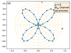
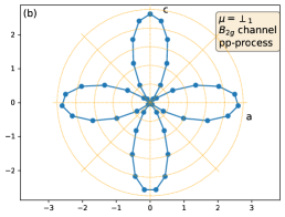
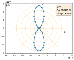
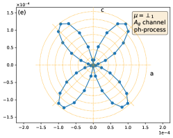
Figure 6: The angular dependence of sound attenuation coefficient $\alpha_{s}^{\mu}(\theta_{\mathbf{q}},\phi_{\mathbf{q}}\!=\!0^{\circ})$ in the $ac$-plane. The pp-processes contribute to (a) the attenuation of the longitudinal phonon ($\alpha_{s}^{\|}$) in $B_{2g}$ channel, (b) the attenuation of the in-plane transverse phonon ($\alpha_{s}^{\perp_{1}}$) in the $B_{2g}$ channel, (c) the attenuation of the out-of-plane transverse phonon ($\alpha_{s}^{\perp_{2}}$) in the $B_{3g}$ channel. The ph-processes contribute to (d) the attenuation of the longitudinal phonon ($\alpha_{s}^{\|}$) and (e) of the in-plane transverse phonon ($\alpha_{s}^{\perp_{1}}$) in the $A_{g}$ channel. The radius represents the magnitude of $\alpha_{s}^{\mu}$ in the units of $10^{-5}\rho\delta_{V}$. The calculation is performed at $T=0.02\,J$.

IV.2 Numerical results

Considering the estimations above, we set $v_{s}^{\|}=3\,J\ell$ and $v_{s}^{\perp_{1,2}}\approx 1.6\,J\ell$. We also take $T=0.02\,J$, which is below the flux energy gap. In the long wavelength limit, the angular dependence of the sound attenuation coefficient is scale invariant and is more experimentally relevant than the dependence on the magnitude of the momentum $q$. Thus, we fix $q=0.005\,\ell^{-1}$ and show the polar plots of the angular dependence of the sound attenuation (where the radius represents the magnitude of the sound attenuation coefficient). This angular dependence is a direct reflection of the Majorana-phonon couplings (II.3) constructed based on symmetry.

We compute the sound attenuation coefficient in the four symmetry channels, $A_{g},B_{1g},B_{2g},B_{3g}$, considering separately the contributions from the pp- and ph-scattering processes. In Figs. 5, 6 and 7, we present our results for the sound attenuation’s angular dependence patterns for the phonon modes in the three crystallographic planes, correspondingly, $ab$, $ac$ and $bc$, for three phonon’s polarizations, $\|,\perp_{1},\perp_{2}$. The explicit expressions for the Majoarana-phonon coupling vertices in these special geometries are presented in Appendix B. These expressions show that for each of the phonon polarizations, the coupling vertex has contributions from only two symmetry channels and another two symmetry channels give exactly zero contribution. Furthermore, we find that some symmetry channels have higher order (dominant) contributions in the long wavelength limit $q\to 0$. So, below we will only show the results from the leading order contributions into sound attenuation for each crystallographic plane.

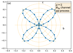
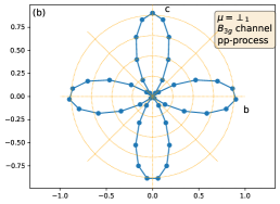
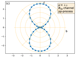
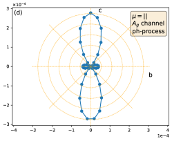
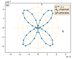
Figure 7: The angular dependence of sound attenuation coefficient $\alpha_{s}^{\mu}(\theta_{\mathbf{q}},\phi_{\mathbf{q}}\!=\!90^{\circ})$ in the $bc$-plane. The pp-processes contribute to (a) the attenuation of the longitudinal phonon ($\alpha_{s}^{\|}$) in $B_{3g}$ channel, (b) the attenuation of the in-plane transverse phonon ($\alpha_{s}^{\perp_{1}}$) in the $B_{3g}$ channel, (c) the attenuation of the out-of-plane transverse phonon ($\alpha_{s}^{\perp_{2}}$) in the $B_{2g}$ channel. The ph-processes contribute to (d) the attenuation of the longitudinal phonon $(\alpha_{s}^{\|}$) and (e) of the in-plane transverse phonon ($\alpha_{s}^{\perp_{1}}$) in the $A_{g}$ channel. The radius represents the magnitude of $\alpha_{s}^{\mu}$ in the units of $10^{-5}\rho\delta_{V}$. The calculation is performed at $T=0.02\,J$.

Phonon within the $ab$ plane.– The contributions from the pp- and ph-scattering processes for the attenuation coefficient for the phonon propagating in the $ab$ plane are shown in Fig. 5 (a)-(c) and (d), (e), respectively. This plane is special compared with $bc$ and $ac$ planes, because of the presence of the nodal line in the fermionic spectrum [see Fig. 2 (a)] as well as the crystallographic structure shown in Fig. 1. As such, there always exist zero Fermi velocities along the nodal line and small Fermi velocities in the vicinity of the nodal line. Therefore, the sound velocities along these directions are larger than the Fermi velocities, which gives rise to the non-zero pp-processes. In this scattering geometry, the pp-processes contribute only in the attenuation of the out-of-plane transverse phonon mode in the $\perp_{2}$ polarization, $\alpha^{\perp_{2}}_{s}(\mathbf{q})$. As follows from Eq. (43), $\alpha^{\perp_{2}}_{s}(\mathbf{q})$ has two contributions, one from the $B_{2g}$ channel [Fig. 5 (a)], describing the attenuation of lattice vibrations in the $ac$-plane, and from the $B_{3g}$ channel [Fig. 5 (b)], describing the attenuation of lattice vibrations in the $bc$-plane, with the former being a bit stronger. The total sound attenuation of the out-of-plane transverse phonon mode $\alpha^{\perp_{2}}_{s}(\mathbf{q})$ shown in Fig. 5 (c) is the sum of these two contributions, and its angular dependence looks like two-fold symmetric four-petal pattern.

Since $v_{s}^{\|}\lesssim\max(v_{F})$ and $v_{s}^{\perp_{1,2}}<\max(v_{F})$, the ph-processes are also allowed. They contribute to the attenuation of the longitudinal phonon mode, $\alpha^{\|}_{s}(\mathbf{q})$, shown in Fig. 5 (d) and of the in-plane transverse mode, $\alpha^{\perp_{1}}_{s}(\mathbf{q})$ shown in Fig. 5 (e). According to the form of Majoarana-phonon coupling vertices in this geometry given by Eq. (41) and Eq. (42), the attenuation of both the longitudinal and the in-plane transverse phonons comes from the dominant $A_{g}$ and subdominant $B_{1g}$ channels. However, at $T=0.02\,J$ both contributions are very small compared with the one from the pp-proecesses. Thus in Fig. 5 (d) and (e) we only show the angular dependence of the attenuation computed from the $A_{g}$ contribution, which displays a vertical dumbbell pattern for $\alpha^{\|}_{s}(\mathbf{q})$, and the diagonal four-petal pattern for $\alpha^{\perp_{1}}_{s}(\mathbf{q})$.

Note, however, that the comparison of the magnitude of the sound attenuation coefficients between ph- and pp- processes needs to take into consideration the temperature effect Feng et al. (2021). Since the pp-processes do not require finite particle number, the low-temperature scaling behaviour of its contribution to the sound attenuation coefficient doesn’t depend on temperature, i.e. $\alpha^{\text{pp}}_{s}\sim T^{0}$. The ph-processes require finite particle occupation, and its low-temperature scaling behaviour is $\alpha^{\text{ph}}_{s}\sim T^{1}$ same as in the 2D Kitaev model Ye et al. (2020). This is a direct result of the fact that the low-energy $\textmd{DOS}(E)\sim E^{1}$ as shown in Fig. 2(c). This low-energy scaling behaviour of DOS can also be analytically obtained by evaluating $\textmd{DOS}(E)=\int_{\textmd{BZ}}\mathrm{d}^{3}\mathbf{k}\,\delta(E-\varepsilon_{\mathbf{k}})$. Then at low energy, if we expand the fermionic spectrum around the nodal line, then

$$\textmd{DOS}(E)=\int_{\textmd{BZ}}\mathrm{d}^{3}\mathbf{k}\,\delta(E-v_{F}(k_{\phi},\delta k_{\theta})\,\delta k_{r}),$$ (24)

where $k_{\phi}$ uniquely specifies a point on the nodal line by its orientation $\phi$. Around this nodal point, on a neighboring disk locally perpendicular to the nodal line, $(\delta k_{\theta},\delta k_{r})$ uniquely specifies the $\mathbf{k}$ point that contributes to the DOS. Then the integration Eq. (24) is equivalent to stringing the local disks together along the nodal line. So it is easy to see that the low-energy scaling behaviour of $\textmd{DOS}(E)$ is decided by the co-dimension, i.e. the dimension of the BZ space minus the nodal dimension. Thus, the low-energy behaviour of $\text{DOS}(E)\sim E^{1}$ is the same for both 2D plane model and 3D hyperhoneycomb model, so is the low-temperature behaviour of the sound attenuation coefficient.

The low-temperature behaviours of both pp- and ph-processes distinguish themselves from the attenuation of other interaction channels, such as the channel due to phonon-phonon interactions which scales as as $\sim T^{3}$ in 2D and $\sim T^{5}$ in 3D, so they are promising for experimental detection at low enough temperature.

Our numerical calculation shows that, even though the temperature dependence of attenuation from ph-process has larger power than that from pp-process, pp-process still dominates at high temperatures. The main reason is that Fermi velocities range from $0$ to $\max(v_{F})=3J\ell$, so the sound velocities $v_{s}^{\|}=3\,J\ell$ and $v_{s}^{\perp_{1,2}}\approx 1.6\,J\ell$, which we use to describe the phonons in $\beta$-Li₂IrO₃ compound, are still larger than a significant portion of Fermi velocities, which is consistent with an existence of the nearly-zero Fermi velocities along the nodal line. If we use fictitious smaller sound velocities, the contribution from the ph-processes will become larger Feng et al. (2021).

Phonon within the $ac$ or $bc$ planes.– As shown in Fig. 6 and Fig. 7, the attenuation of the phonons propagating in the $ac$ and $bc$ planes are similar, which is consistent with the crystallographic structure displayed in Fig. 1. Because the Fermi velocities for small deviations ${\bf k}$ from the nodal line ${\bf K}_{0}=(k_{a},k_{b},0)$ either into the $ac$ or into the $bc$ planes are small, at low temperatures the pp-processes dominate over the ph-processes and thus define the angular dependence of the sound attenuation. In both geometries, the pp-processes contribute to the attenuation of the phonons with all three different polarizations angular, with similar angular patters. However, while for the phonon in the $ac$ plane, the strongest attenuation is for the in-plane transverse phonon ($\alpha_{s}^{\perp_{1}}$), for the phonon in the $bc$ plane, the strongest attenuation is for out-of-plane transverse polarization ($\alpha_{s}^{\perp_{2}}$). In both geometries, attenuation of phonons with out-of-plane transverse polarization only happen through pp-processes and displays the vertical dumbbell pattern. The four-petal angular patterns of attenuation of the longitudinal and the in-plane transverse phonons are rotated by 45^∘ with respect to each other. As mentioned before, these distinct patterns directly reflect the spin-phonon couplings from different symmetry channels, probed by different phonon polarization modes. The temperature dependence of the sound attenuation of the phonons propagating in $ac$ or $bc$ planes is similar to that in $ab$ plane.

V Summary

In this paper, we studied the three-dimensional Kitaev spin-phonon model on the hyperhoneycomb lattice. In this model, the sound attenuation is determined by the decay of a phonon into a pair of Majorana fermions and can be calculated from the imaginary part of the phonon self-energy, which at the lowest order is given by the polarization bubble. Thus, we argued that the phonon attenuation, measurable by the ultrasound experiments, can serve as an effective indirect probe of the spin fractionalization.

In our work we considered only low temperatures below the flux disordering transition Nasu et al. (2014b), in which only Majorana fermions contribute to the phonon self-energy. We showed that Majorana semimetal with nodal line band structure leaves distinct characteristic fingerprints in the temperature dependence of the phonon attenuation coefficient as a function of incident phonon momentum. First, it allows the presence of the pp-processes of the phonon decay in all three considered scattering geometries with the phonon propagating in one of the three crystallographic planes. Second, since the pp-processes of the phonon decay is allowed at all temperatures, the sound attenuation is non zero even at zero temperature and is almost temperature independent ($\sim T^{0}$) at lowest temperatures. Combining both pp-processes and ph-processes that are allowed by symmetry constraints for each scattering geometry and phonon polarization, the temperature dependence of attenuation coefficient can be schematically described by $a_{T}T^{0}+b_{T}T^{1}$ with $a_{T}>b_{T}$. Thus, the sound attenuation contributed from the decay into fractionalized excitations will be the dominant one at low enough temperatures, distinguishing itself from the contribution due to the phonon-phonon interactions, which scales as $\varpropto T^{5}$ in the three-dimensional system. We anticipate that the $Z_{2}$ fluxes will play an important role on the phonon dynamics at temperatures above the flux ordering transition temperature. We also obtained that the sound attenuation shows a strong angular dependence at the leading order in phonon momentum $q$. It is determined by the anisotropic form of the MFPh coupling and the nodal structure of the low-energy fermionic excitations.

Finally, we note that our study was performed for the pure Kitaev model. Of course, real Kitaev materials feature additional weak time-reversal-invariant non-Kitaev interactions, which give rise to other magnetic phases competing with the Kitaev spin liquid. In particular, the minimal spin Hamiltonian for the $\beta$-Li₂IrO₃ compound in addition to the Kitaev coupling has contains antiferromagnetic Heisenberg interaction and off-diagonal $\Gamma$ exchange term Ducatman et al. (2018). Nevertheless, we believe that the temperature evolution of the sound attenuation will remain similar to the one in the pure Kitaev model as long as these perturbations do not break time reversal symmetry protecting the nodal line O’Brien et al. (2016) and are small enough that the material is in the proximity to the spin liquid phase.

Acknowledgments: We thank Rafael Fernandes, Gabor Halasz and Mengxing Ye for earlier collaborations related to the topic of this study. The work of K.F. and N.B.P. was supported by the U.S. Department of Energy, Office of Science, Basic Energy Sciences under Award No. DE-SC0018056.

Appendix A Details of the MFPh coupling’s derivation

In this appendix we present the technical details of the derivation of the Majorana fermion-phonon (MFPh) coupling. In the momentum space, the Majorana-phonon coupling Hamiltonian is can be written as

$${\mathcal{H}}^{c}=\sqrt{\frac{2}{N}}\sum_{{\bf q},{\bf k}}({\mathcal{H}}_{{\bf q},{\bf k}}^{A_{g}}+{\mathcal{H}}_{{\bf q},{\bf k}}^{B_{1g}}+{\mathcal{H}}_{{\bf q},{\bf k}}^{B_{2g}}+{\mathcal{H}}_{{\bf q},{\bf k}}^{B_{3g}}),$$ (25)

where the explicit expressions for the contributions from different symmetry channels are given by

$${\mathcal{H}}_{{\bf q},\bf{k}}^{A_{g}}=i{\lambda_{A_{g}}}\bigg{(}4q_{c}u_{{\bf q},c}{\bf A}^{\mkern-1.5mu\mathsf{T}}_{-{\bf q}-\bf{k}}S_{\bf{k}}^{\dagger}\begin{pmatrix}\hat{O}&-i\hat{\sigma}_{3}\\ i\hat{\sigma}_{3}&\hat{O}\end{pmatrix}S_{\bf k}{\bf A}_{\bf k}+(q_{c}u_{{\bf q},c}+2q_{b}u_{{\bf q},b}+q_{a}u_{{\bf q},a}){\bf A}^{\mkern-1.5mu\mathsf{T}}_{{-{\bf q}-{\bf k}}}S_{\bf k}^{\dagger}\hat{Q}_{{\bf k},1}S_{\bf k}{\bf A}_{\bf k}\bigg{)},$$

$${\mathcal{H}}_{{\bf q},{\bf k}}^{B_{1g}}=\frac{i{\lambda_{B_{1g}}}}{2}(q_{a}u_{{\bf q},b}+q_{b}u_{{\bf q},a})\,{\bf A}^{\mkern-1.5mu\mathsf{T}}_{-{\bf q}-{\bf k}}S_{\bf k}^{\dagger}\hat{Q}_{{\bf k},2}S_{\bf{k}}{\bf A}_{\bf k},$$

$${\mathcal{H}}_{{\bf q},{\bf k}}^{B_{2g}}=\frac{i{\lambda_{B_{2g}}}}{2}(q_{a}u_{{\bf q},c}+q_{c}u_{{\bf q},a})\,{\bf A}_{-{\bf q}-{\bf k}}^{\mkern-1.5mu\mathsf{T}}S_{\bf k}^{\dagger}\hat{Q}_{{\bf k},3}S_{\bf k}{\bf A}_{\bf k},$$

$${\mathcal{H}}_{{\bf q},{\bf k}}^{B_{3g}}=\frac{i{\lambda_{B_{3g}}}}{2}(q_{b}u_{{\bf q},c}+q_{c}u_{{\bf q},b})\,{\bf A}^{\mkern-1.5mu\mathsf{T}}_{-{\bf q}-{\bf k}}S_{\bf k}^{\dagger}\hat{Q}_{{\bf k},4}S_{\bf k}{\bf A}_{\bf k}.$$

Here $S_{\bf{k}}={\rm diag}\{e^{i\bf{k}\cdot{\bf r}_{\alpha}}\}_{\alpha=C,B,D,A}$ is the diagonal matrix in the sublattice basis, $\hat{O}=\begin{pmatrix}0&0\\ 0&0\end{pmatrix}$ is the zero 2 by 2 matrix, $\hat{\sigma_{i}}$ are the auxiliary Pauli matrices, and the explicit expressions for $\hat{Q}_{{\bf k}}$-matrices are given by

$$\hat{Q}_{{\bf k},1}=\left(\begin{array}[]{cc}(1+\cos({\bf k}\cdot{\bf a}_{3}))\hat{\sigma_{2}}+\sin({\bf k}\cdot{\bf a}_{3})\hat{\sigma_{1}}&\hat{O}\\ \hat{O}&-(\cos({\bf k}\cdot{\bf a}_{1})+\cos({\bf k}\cdot{\bf a}_{2}))\hat{\sigma_{2}}-(\sin({\bf k}\cdot{\bf a}_{1})+\sin({\bf k}\cdot{\bf a}_{2}))\hat{\sigma_{1}}\end{array}\right),$$ (28)

$$\hat{Q}_{{\bf k},2}=\left(\begin{array}[]{cc}(1+\cos({\bf k}\cdot{\bf a}_{3}))\hat{\sigma_{2}}+\sin({\bf k}\cdot{\bf a}_{3})\hat{\sigma_{1}}&\hat{O}\\ \hat{O}&(\cos({\bf k}\cdot{\bf a}_{1})+\cos({\bf k}\cdot{\bf a}_{2}))\hat{\sigma_{2}}+(\sin({\bf k}\cdot{\bf a}_{1})+\sin({\bf k}\cdot{\bf a}_{2}))\hat{\sigma_{1}}\end{array}\right),$$ (31)

$$\hat{Q}_{{\bf k},3}=\left(\begin{array}[]{cc}(1-\cos({\bf k}\cdot{\bf a}_{3}))\hat{\sigma_{2}}-\sin({\bf k}\cdot{\bf a}_{3})\hat{\sigma_{1}}&\hat{O}\\ \hat{O}&(\cos({\bf k}\cdot{\bf a}_{1})-\cos({\bf k}\cdot{\bf a}_{2}))\hat{\sigma_{2}}+(\sin({\bf k}\cdot{\bf a}_{1})-\sin({\bf k}\cdot{\bf a}_{2}))\hat{\sigma_{1}}\end{array}\right),$$ (34)

$$\hat{Q}_{{\bf k},4}=\left(\begin{array}[]{cc}(1-\cos({\bf k}\cdot{\bf a}_{3}))\hat{\sigma_{2}}-\sin({\bf k}\cdot{\bf a}_{3})\hat{\sigma_{1}}&\hat{O}\\ \hat{O}&(\cos({\bf k}\cdot{\bf a}_{2})-\cos({\bf k}\cdot{\bf a}_{1}))\hat{\sigma_{2}}+(\sin({\bf k}\cdot{\bf a}_{2})-\sin({\bf k}\cdot{\bf a}_{1}))\hat{\sigma_{1}}\end{array}\right).$$ (37)

Next we rewrite ${\mathcal{H}}^{c}$ in terms of the transverse and longitudinal eigenmodes as in Eq. (II.3), where corresponding MFPh coupling vertices are given by

$$\hat{\lambda}_{{\bf q},\bf{k}}^{\parallel} =i\lambda_{A_{g}}\bigg{(}{4q_{c}R_{31}\begin{pmatrix}\hat{O}&-i\hat{\sigma}_{3}\\ i\hat{\sigma}_{3}&\hat{O}\end{pmatrix}+(q_{c}R_{31}+2q_{b}R_{21}+q_{a}R_{11})\,\hat{Q}_{{\bf k},1}}\bigg{)}$$ (38)

$$+\frac{i\lambda_{B_{1g}}}{2}(q_{a}R_{21}+q_{b}R_{11})\,\hat{Q}_{{\bf k},2}+\frac{i\lambda_{B_{2g}}}{2}(q_{a}R_{31}+q_{c}R_{11})\,\hat{Q}_{{\bf k},3}+\frac{i\lambda_{B_{3g}}}{2}(q_{b}R_{31}+q_{c}R_{21})\,\hat{Q}_{{\bf k},4},$$

$$\hat{\lambda}_{{\bf q},\bf{k}}^{\perp_{1}} =i\lambda_{A_{g}}\bigg{(}{4q_{c}R_{32}\begin{pmatrix}\hat{O}&-i\hat{\sigma}_{3}\\ i\hat{\sigma}_{3}&\hat{O}\end{pmatrix}+(q_{c}R_{32}+2q_{b}R_{22}+q_{a}R_{12})\,\hat{Q}_{{\bf k},1}}\bigg{)}$$ (39)

$$+\frac{i\lambda_{B_{1g}}}{2}(q_{a}R_{22}+q_{b}R_{12})\,\hat{Q}_{{\bf k},2}+\frac{i\lambda_{B_{2g}}}{2}(q_{a}R_{32}+q_{c}R_{12})\,\hat{Q}_{{\bf k},3}+\frac{i\lambda_{B_{3g}}}{2}(q_{b}R_{32}+q_{c}R_{22})\,\hat{Q}_{{\bf k},4},$$

$$\hat{\lambda}_{{\bf q},\bf{k}}^{\perp_{2}} =i\lambda_{A_{g}}\bigg{(}{4q_{c}R_{33}\begin{pmatrix}\hat{O}&-i\hat{\sigma}_{3}\\ i\hat{\sigma}_{3}&\hat{O}\end{pmatrix}+(q_{c}R_{33}+2q_{b}R_{23}+q_{a}R_{13})\,\hat{Q}_{{\bf k},1}}\bigg{)}$$ (40)

$$+\frac{i\lambda_{B_{1g}}}{2}(q_{a}R_{23}+q_{b}R_{13})\,\hat{Q}_{{\bf k},2}+\frac{i\lambda_{B_{2g}}}{2}(q_{a}R_{33}+q_{c}R_{13})\,\hat{Q}_{{\bf k},3}+\frac{i\lambda_{B_{3g}}}{2}(q_{b}R_{33}+q_{c}R_{23})\,\hat{Q}_{{\bf k},4}.$$

Note also that since we are using the long wavelength limit for the phonons, we only kept the leading in $q$ terms in all the expressions.

Appendix B MFPh couplings in various polarizations

For phonon in the $ab$ plane, the rotation matrix is given by $\hat{R}=\left[\begin{array}[]{ccc}\cos\phi_{\mathbf{q}}&-\sin\phi_{\mathbf{q}}&0\\ \sin\phi_{\mathbf{q}}&\cos\phi_{\mathbf{q}}&0\\ 0&0&1\end{array}\right],$which simplifies the general expressions for the MFPh coupling vertices to

$$\hat{\lambda}_{\mathbf{q},\mathbf{k}}^{\|}= i\lambda_{A_{g}}q_{a}R_{11}\hat{Q}_{\mathbf{k},1}+\frac{i\lambda_{B_{1g}}}{2}\left(q_{a}R_{21}+q_{b}R_{11}\right)\hat{Q}_{\mathbf{k},2},$$ (41)

$$\hat{\lambda}_{\mathbf{q},\mathbf{k}}^{\perp_{1}}= i\lambda_{A_{g}}\left(2q_{b}R_{22}+q_{a}R_{12}\right)\hat{Q}_{\mathbf{k},1}+\frac{i\lambda_{B_{1g}}}{2}\left(q_{a}R_{22}+q_{b}R_{12}\right)\hat{Q}_{\mathbf{k},2}$$ (42)

$$\hat{\lambda}_{\mathbf{q},\mathbf{k}}^{\perp_{2}}= \frac{i\lambda_{B_{2g}}}{2}q_{a}R_{33}\hat{Q}_{\mathbf{k},3}+\frac{i\lambda_{B_{3g}}}{2}q_{b}R_{33}\hat{Q}_{\mathbf{k},4}.$$ (43)

Similarly, for the phonon in the $ac$ plane, the rotation matrix is given by $\hat{R}=\left[\begin{array}[]{ccc}\sin\theta_{\mathbf{q}}&\cos\theta_{\mathbf{q}}&0\\ 0&0&1\\ \cos\theta_{\mathbf{q}}&-\sin\theta_{\mathbf{q}}&0\end{array}\right]$, so the MFPh coupling vertices are given by

$$\hat{\lambda}_{\mathbf{q},\mathbf{k}}^{\|}= i\lambda_{A_{g}}\left(4q_{c}R_{31}\left(\begin{array}[]{cc}\hat{O}&-i\hat{\sigma}_{3}\\ i\hat{\sigma}_{3}&\hat{O}\end{array}\right)+\left(q_{c}R_{31}+q_{a}R_{11}\right)\hat{Q}_{\mathbf{k},1}\right)+\frac{i\lambda_{B_{2g}}}{2}\left(q_{a}R_{31}+q_{c}R_{11}\right)\hat{Q}_{\mathbf{k},3},$$ (46)

$$\hat{\lambda}_{\mathbf{q},\mathbf{k}}^{\perp_{1}}= i\lambda_{A_{g}}\left(4q_{c}R_{32}\left(\begin{array}[]{cc}\hat{O}&-i\hat{\sigma}_{3}\\ i\hat{\sigma}_{3}&\hat{O}\end{array}\right)+\left(q_{c}R_{32}+q_{a}R_{12}\right)\hat{Q}_{\mathbf{k},1}\right)+\frac{i\lambda_{B_{2g}}}{2}\left(q_{a}R_{32}+q_{c}R_{12}\right)\hat{Q}_{\mathbf{k},3},$$ (49)

$$\hat{\lambda}_{\mathbf{q},\mathbf{k}}^{\perp_{2}}= \frac{i\lambda_{B_{1g}}}{2}q_{a}R_{23}\hat{Q}_{\mathbf{k},2}+\frac{i\lambda_{B_{3g}}}{2}q_{c}R_{23}\hat{Q}_{\mathbf{k},4}.$$ (50)

For the phonon in the $bc$ plane, the rotation matrix is $\hat{R}=\left[\begin{array}[]{ccc}0&0&1\\ \sin\theta_{\mathbf{q}}&\cos\theta_{\mathbf{q}}&0\\ \cos\theta_{\mathbf{q}}&-\sin\theta_{\mathbf{q}}&0\end{array}\right]$ , and the MFPh coupling vertices are given by

$$\hat{\lambda}_{\mathbf{q},\mathbf{k}}^{\|}= i\lambda_{A_{g}}\left(4q_{c}R_{31}\left(\begin{array}[]{cc}\hat{O}&-i\hat{\sigma}_{3}\\ i\hat{\sigma}_{3}&\hat{O}\end{array}\right)+\left(q_{c}R_{31}+2q_{b}R_{21}\right)\hat{Q}_{\mathbf{k},1}\right)+\frac{i\lambda_{B_{3g}}}{2}\left(q_{b}R_{31}+q_{c}R_{21}\right)\hat{Q}_{\mathbf{k},4},$$ (53)

$$\hat{\lambda}_{\mathbf{q},\mathbf{k}}^{\perp_{1}}= i\lambda_{A_{g}}\left(4q_{c}R_{32}\left(\begin{array}[]{cc}\hat{O}&-i\hat{\sigma}_{3}\\ i\hat{\sigma}_{3}&\hat{O}\end{array}\right)+\left(q_{c}R_{32}+2q_{b}R_{22}\right)\hat{Q}_{\mathbf{k},1}\right)+\frac{i\lambda_{B_{3g}}}{2}\left(q_{b}R_{32}+q_{c}R_{22}\right)\hat{Q}_{\mathbf{k},4},$$ (56)

$$\hat{\lambda}_{\mathbf{q},\mathbf{k}}^{\perp_{2}}= \frac{i\lambda_{B_{1g}}}{2}q_{b}R_{13}\hat{Q}_{\mathbf{k},2}+\frac{i\lambda_{B_{2g}}}{2}q_{c}R_{13}\hat{Q}_{\mathbf{k},3}.$$ (57)

So in each plane, only two of the fours symmetry channels are active. And as shown in the numerical calculations presented in the main text, in the long wavelength limit, one of the two channels dominates over the other. Similar situation was observed in the analysis of the 2D spin-phonon Kitaev model Ye et al. (2020).

Appendix C Explicit expressions for the dynamical factors in (20)

The dynamic factors in Eq. (20) are evaluated as follows:

$$P_{\mathbf{k},11} =T\sum_{i\omega_{m}}\frac{1}{\left(i\Omega_{n}+i\omega_{m}\right)-\varepsilon_{\mathbf{k}}}\frac{1}{i\omega_{m}-\varepsilon_{\mathbf{k}+\mathbf{q}}}=\frac{n_{F}\left(\varepsilon_{\mathbf{k}}\right)-n_{F}\left(\varepsilon_{\mathbf{k}+\mathbf{q}}\right)}{i\Omega_{n}-\varepsilon_{\mathbf{k}}+{\varepsilon_{\mathbf{k}+\mathbf{q}}}},$$

$$P_{\mathbf{k},22} =T\sum_{i\omega_{m}}\frac{1}{\left(i\Omega_{n}+i\omega_{m}\right)+\varepsilon_{\mathbf{k}}}\frac{1}{i\omega_{m}+\varepsilon_{\mathbf{k}+\mathbf{q}}}=\frac{n_{F}\left(-\varepsilon_{\mathbf{k}}\right)-n_{F}\left(-\varepsilon_{\mathbf{k}+\mathbf{q}}\right)}{i\Omega_{n}+\varepsilon_{\mathbf{k}}-\varepsilon_{\mathbf{k}+\mathbf{q}}},$$ (58)

$$P_{\mathbf{k},21} =T\sum_{i\omega_{m}}\frac{1}{\left(i\Omega_{n}+i\omega_{m}\right)+\varepsilon_{\mathbf{k}}}\frac{1}{i\omega_{m}-\varepsilon_{\mathbf{k}+\mathbf{q}}}=\frac{n_{F}\left(-\varepsilon_{\mathbf{k}}\right)-n_{F}\left(\varepsilon_{\mathbf{k}+\mathbf{q}}\right)}{i\Omega_{n}+\varepsilon_{\mathbf{k}}+\varepsilon_{\mathbf{k}+\mathbf{q}}},$$ (59)

$$P_{\mathbf{k},12} =T\sum_{i\omega_{m}}\frac{1}{\left(i\Omega_{n}+i\omega_{m}\right)-\varepsilon_{\mathbf{k}}}\frac{1}{i\omega_{m}+\varepsilon_{\mathbf{k}+\mathbf{q}}}=\frac{n_{F}\left(\varepsilon_{\mathbf{k}}\right)-n_{F}\left(-\varepsilon_{\mathbf{k}+\mathbf{q}}\right)}{i\Omega_{n}-\varepsilon_{\mathbf{k}}-\varepsilon_{\mathbf{k}+\mathbf{q}}},$$

Appendix D Vegas+ Monte Carlo integration

In this paper, we applied an efficient Monte Carlo algorithm for multidimensional integration Vegas+ Lepage (2021); Dehesa et al. (2011) to evaluate the phase space integration in the polarization bubble Eq. (III). In this section, we will briefly discuss the technical aspect of this algorithm.

Vegas+ is an adaptive stratified sampling algorithm, which is very effective for the integrands with multiple peaks or diagonal nodal (significant) structures. In general, an importance sampling (as in the original Vegas algorithm) is a basic variance reduction technique in Monte Carlo integration, where the probability space is transformed, such that the sampling is concentrated on the important region of the integrand. For example, suppose we need to compute a 1D integral

$$I=\int_{a}^{b}f(x)\mathrm{d}x.$$ (60)

Different from directly sampling $x\in[a,b]$, as is done in a standard Monte Carlo technique, importance sampling introduces a measurable map from $y$ to $x$, $x=G^{-1}(y)$, where $y\in[0,1]$. Then, the integration is equivalently written as:

$$I=\int_{0}^{1}f(x(y))\frac{\mathrm{d}x}{\mathrm{d}y}\mathrm{d}y,$$ (61)

and, instead of uniformly sampling $x\in[a,b]$, one uniformly samples $y\in[0,1]$. The result of this probability space transformation is such that the distribution of $x$ is described by function $g(x)=G^{\prime}(x)$ (known from inverse transform sampling). If $g(x)$ is well designed to be of similar shape to $f(x)$, i.e. $g(x)$ is large where $f(x)$ is large, then the $x$ samples will be concentrated in the important region of $f(x)$.

What the Vegas algorithm Lepage (1978) does is to numerically obtain the map $G^{-1}:y\to x$, which gives the probability distribution function $g(x)$, in the following adaptive way. First the $x$ integration space is partitioned into $N_{p}$ intervals, and $\Delta x_{i}$ is the length of each interval (not necessarily uniform). Then the functional form is chosen such that $x$ monotonically increases with $y$, and within each partition of $x$, the increase is linear with a rate (Jacobian) $J_{i}$, i.e. $\Delta x_{i}=J_{i}\Delta y_{i}$, (again not necessarily uniform). So the measurable map $G^{-1}:y\to x$ is specified by the set of variables $\{\Delta x_{i},J_{i}\}$, which are under the constraints $\sum_{i=1}^{N_{p}}\Delta x_{i}=b-a$, $\sum_{i=1}^{N_{p}}\Delta y_{i}=1$. The objective of designing the distribution function $g(x)$ is to minimize the variation of the integrand (seen as a function of random variable $y$):

$$\sigma_{I}^{2}=\mathbb{V}\textmd{ar}_{y\in[0,1]}\left[f(x(y))\frac{\mathrm{d}x}{\mathrm{d}y}\right]=\int_{0}^{1}\left[f(x(y))\frac{\mathrm{d}x}{\mathrm{d}y}\right]^{2}\mathrm{d}y-I^{2}=\sum_{i}J_{i}\int_{x_{i}}^{x_{i}+\Delta x_{i}}f(x)^{2}\mathrm{d}x-I^{2},$$ (62)

where $x_{i}$ is the left end of each interval partitioned from $x\in[a,b]$. So now designing the map $G^{-1}:y\to x$ becomes a constrained optimization problem

$$\min_{\{\Delta x_{i},J_{i}\}}\sigma_{I}^{2}\left(\{\Delta x_{i},J_{i}\}\right).$$ (63)

From here, it is easy to get the necessary optimal condition Lepage (2021):

$$\frac{1}{\Delta x_{i}}\int_{x_{i}}^{x_{i}+\Delta x_{i}}J_{i}^{2}f(x)^{2}\mathrm{d}x=\textmd{constant},$$ (64)

i.e. the optimal partition grid $\{x_{i}\}$ is such that the average of $J_{i}^{2}f(x)^{2}$ over each interval $\Delta x_{i}$ is uniform across the partitions. Without loss of generality, we can introduce uniform grid (partition) in $y$ space, i.e. $\Delta y_{i}=1/N_{p}$. Then, $J_{i}=\frac{\Delta x_{i}}{\Delta y_{i}}=\Delta x_{i}\cdot N_{p}$. Then, the objective becomes finding the grid in $x$ space, such that the average of $\Delta x_{i}^{2}f(x)^{2}$ over $\Delta x_{i}$ is uniform, the result of which leads to importance sampling.

The uniform $\Delta x_{i}^{2}f(x)^{2}$ is achieved by an adaptive numerical algorithm, which can be intuitively understood as follows. First, the average $w_{i}=\left\langle\Delta x_{i}^{2}f(x)^{2}\right\rangle_{\Delta x_{i}}$ on $\Delta x_{i}$ is defined to be the weight of the $i$-th partition. We also define the center weight of all partitions to be $c=\frac{1}{N_{p}}\sum_{i}w_{i}$. Then the uniform weight $\{w_{i}\}$ condition is equivalent to requiring $\sum_{i}\left|w_{i}-c\right|^{2}$ to be minimized. In other words, we have the following optimization problem:

$$L(\{x_{i}\})=\min_{\{x_{i}\}}\min_{c}\sum_{i}\left|w_{i}-c\right|^{2}$$ (65)

We can easily verify that uniform $\{w_{i}\}$ is indeed the saddle point solution, i.e., if $\{w_{i}\}$ is uniform, then $L=0$. This problem is solved by an alternating optimization algorithm, which alternatively updates $\{x_{i}\}$ and $c$ in an adaptive procedure Lepage (2021). The optimal solution yields a grid of $x$, which is the most dense in the importance region of the integrand. Thus Vegas is considered an adaptive importance sampling method.

Next, we introduce vegas+, the enhanced version of vegas with stratified sampling. In the above algorithm, we have obtained the the uniform grid of $\{y_{i}=1/N_{p}\}$, so it is natural to stratify the sampling according this partition. To obtain the optimal number of samples allocated to each stratum $\{n_{i}\}$, we can minimize the Monte Carlo standard deviation $\sigma_{\textmd{MC}}^{2}=\sum_{i=1}^{N_{p}}\frac{\sigma^{2}_{i}(fJ_{i})}{n_{i}}$ with the constraint $\sum_{i}n_{i}=N_{total}$, where $\sigma_{i}(fJ_{i})$ is the variance of $f(x)J_{i}$ in the $i$-th partition. This gives that the optimal stratification is $n_{i}\propto\sigma_{i}(fJ_{i})$. The same optimization method was also applied in the stratified Monte Carlo simulations in the 2D Kitaev QSL  Feng et al. (2021); Feng (2022), except that there $\sigma_{\textmd{MC}}^{2}=\sum_{i}\frac{p_{i}^{2}\sigma_{i}^{2}}{n_{i}}$, where $p_{i}$ is the normalized probability of the $i$-th partition, and the optimal stratification is $n_{i}\propto p_{i}\sigma_{i}\approx p_{i}$.

Finally, in this paper the integration was done in 3D ${\bf k}$-space with the important region centered around the nodal line. The Vegas algorithm was used to make sure that the samples are concentrated near the 2D plane. But within that 2D plane, partition grid is basically uniform. At this point, the adaptive stratified sampling of Vegas+ was used to assure that the dominant contribution comes from the samples only in the important hypercubes near the nodal line.

References

- Lee (2008) P. A. Lee, Science 321, 1306 (2008).
- Balents (2010) L. Balents, Nature 464, 199 (2010).
- Savary and Balents (2017) L. Savary and L. Balents, Rep. Prog. Phys. 80, 016502 (2017).
- Zhou et al. (2017) Y. Zhou, K. Kanoda, and T.-K. Ng, Rev. Mod. Phys. 89, 025003 (2017).
- Knolle and Moessner (2019) J. Knolle and R. Moessner, Annu. Rev. Condens. Matter Phys. 10, 451 (2019).
- Broholm et al. (2020) C. Broholm, R. J. Cava, S. A. Kivelson, D. G. Nocera, M. R. Norman, and T. Senthil, Science 367 (2020).
- Motome and Nasu (2020) Y. Motome and J. Nasu, J. Phys. Soc. Jpn 89, 012002 (2020).
- Kitaev (2006) A. Kitaev, Annals of Physics 321, 2 (2006).
- Jackeli and Khaliullin (2009) G. Jackeli and G. Khaliullin, Phys. Rev. Lett. 102, 017205 (2009).
- Chaloupka et al. (2010) J. Chaloupka, G. Jackeli, and G. Khaliullin, Phys. Rev. Lett. 105, 027204 (2010).
- Takagi et al. (2019) H. Takagi, T. Takayama, G. Jackeli, G. Khaliullin, and S. E. Nagler, Nat. Rev. Phys. 1, 264 (2019).
- Knolle et al. (2014a) J. Knolle, D. L. Kovrizhin, J. T. Chalker, and R. Moessner, Phys. Rev. Lett. 112, 207203 (2014a).
- Knolle et al. (2014b) J. Knolle, G.-W. Chern, D. L. Kovrizhin, R. Moessner, and N. B. Perkins, Phys. Rev. Lett. 113, 187201 (2014b).
- Knolle et al. (2015) J. Knolle, D. L. Kovrizhin, J. T. Chalker, and R. Moessner, Phys. Rev. B 92, 115127 (2015).
- Perreault et al. (2015) B. Perreault, J. Knolle, N. B. Perkins, and F. J. Burnell, Phys. Rev. B 92, 094439 (2015).
- Perreault et al. (2016) B. Perreault, J. Knolle, N. B. Perkins, and F. J. Burnell, Phys. Rev. B 94, 104427 (2016).
- Smith et al. (2016) A. Smith, J. Knolle, D. L. Kovrizhin, J. T. Chalker, and R. Moessner, Phys. Rev. B 93, 235146 (2016).
- Halász et al. (2016) G. B. Halász, N. B. Perkins, and J. van den Brink, Phys. Rev. Lett. 117, 127203 (2016).
- Halász et al. (2017) G. B. Halász, B. Perreault, and N. B. Perkins, Phys. Rev. Lett. 119, 097202 (2017).
- Halász et al. (2019) G. B. Halász, S. Kourtis, J. Knolle, and N. B. Perkins, Phys. Rev. B 99, 184417 (2019).
- Eschmann et al. (2020) T. Eschmann, P. A. Mishchenko, K. O’Brien, T. A. Bojesen, Y. Kato, M. Hermanns, Y. Motome, and S. Trebst, Phys. Rev. B 102, 075125 (2020).
- Zhou and Lee (2011) Y. Zhou and P. A. Lee, Phys. Rev. Lett. 106, 056402 (2011).
- Serbyn and Lee (2013) M. Serbyn and P. A. Lee, Phys. Rev. B 87, 174424 (2013).
- Metavitsiadis and Brenig (2020) A. Metavitsiadis and W. Brenig, Phys. Rev. B 101, 035103 (2020).
- Ye et al. (2020) M. Ye, R. M. Fernandes, and N. B. Perkins, Phys. Rev. Research 2, 033180 (2020).
- Feng et al. (2021) K. Feng, M. Ye, and N. B. Perkins, Phys. Rev. B 103, 214416 (2021).
- Metavitsiadis et al. (2021) A. Metavitsiadis, W. Natori, J. Knolle, and W. Brenig, (2021).
- Hentrich et al. (2018) R. Hentrich, A. U. B. Wolter, X. Zotos, W. Brenig, D. Nowak, A. Isaeva, T. Doert, A. Banerjee, P. Lampen-Kelley, D. G. Mandrus, S. E. Nagler, J. Sears, Y.-J. Kim, B. Büchner, and C. Hess, Phys. Rev. Lett. 120, 117204 (2018).
- Kasahara et al. (2018) Y. Kasahara, T. Ohnishi, Y. Mizukami, O. Tanaka, S. Ma, K. Sugii, N. Kurita, H. Tanaka, J. Nasu, Y. Motome, T. Shibauchi, and Y. Matsuda, Nature 559, 227 (2018).
- Pal et al. (2020) S. Pal, A. Seth, P. Sakrikar, A. Ali, S. Bhattacharjee, D. V. S. Muthu, Y. Singh, and A. K. Sood, arXiv:2011.00606 (2020).
- Li et al. (2021) H. Li, T. T. Zhang, A. Said, G. Fabbris, D. G. Mazzone, J. Q. Yan, D. Mandrus, G. B. Halasz, S. Okamoto, S. Murakami, M. P. M. Dean, H. N. Lee, and H. Miao, Nature Communications 12, 3513 (2021).
- Sandilands et al. (2015) L. J. Sandilands, Y. Tian, K. W. Plumb, Y.-J. Kim, and K. S. Burch, Phys. Rev. Lett. 114, 147201 (2015).
- Glamazda et al. (2017) A. Glamazda, P. Lemmens, S.-H. Do, Y. S. Kwon, and K.-Y. Choi, Phys. Rev. B 95, 174429 (2017).
- Mai et al. (2019) T. T. Mai, A. McCreary, P. Lampen-Kelley, N. Butch, J. R. Simpson, J.-Q. Yan, S. E. Nagler, D. Mandrus, A. R. H. Walker, and R. V. Aguilar, Phys. Rev. B 100, 134419 (2019).
- Wulferding et al. (2020) D. Wulferding, Y. Choi, S.-H. Do, C. H. Lee, P. Lemmens, C. Faugeras, and K.-Y. Gallais, Yann andChoi, Nat. Commun. 11, 1603 (2020).
- Lin et al. (2020) D. Lin, K. Ran, H. Zheng, J. Xu, L. Gao, J. Wen, S.-L. Yu, J.-X. Li, and X. Xi, Phys. Rev. B 101, 045419 (2020).
- Feng et al. (2022) K. Feng, S. Swarup, and N. B. Perkins, Phys. Rev. B 105, L121108 (2022).
- Mandal and Surendran (2009) S. Mandal and N. Surendran, Phys. Rev. B 79, 024426 (2009).
- Hermanns and Trebst (2014) M. Hermanns and S. Trebst, Phys. Rev. B 89, 235102 (2014).
- Hermanns et al. (2015) M. Hermanns, K. O’Brien, and S. Trebst, Phys. Rev. Lett. 114, 157202 (2015).
- O’Brien et al. (2016) K. O’Brien, M. Hermanns, and S. Trebst, Phys. Rev. B 93, 085101 (2016).
- Trebst and Hickey (2022) S. Trebst and C. Hickey, Physics Reports 950, 1 (2022).
- Biffin et al. (2014) A. Biffin, R. D. Johnson, I. Kimchi, R. Morris, A. Bombardi, J. G. Analytis, A. Vishwanath, and R. Coldea, Phys. Rev. Lett. 113, 197201 (2014).
- Takayama et al. (2015) T. Takayama, A. Kato, R. Dinnebier, J. Nuss, H. Kono, L. S. I. Veiga, G. Fabbris, D. Haskel, and H. Takagi, Phys. Rev. Lett. 114, 077202 (2015).
- Ruiz et al. (2017) A. Ruiz, A. Frano, N. P. Breznay, I. Kimchi, T. Helm, I. Oswald, J. Y. Chan, R. J. Birgeneau, Z. Islam, and J. G. Analytis, Nature Communications 8, 961 (2017).
- Ruiz et al. (2021) A. Ruiz, N. P. Breznay, M. Li, I. Rousochatzakis, A. Allen, I. Zinda, V. Nagarajan, G. Lopez, Z. Islam, M. H. Upton, et al., Physical Review B 103, 184404 (2021).
- (47) Y. Yang, Y. Wang, I. Rousochatzakis, A. Ruiz, J. G. Analytis, K. S. Burch, and N. B. Perkins, arXiv:2202.00581 .
- (48) T. Halloran, Y. Wang, M. Li, I. Rousochatzakis, P. Chauhan, M. Stone, T. Takayama, N. P. Armitage, N. B. Perkins, and C. Broholm, arXiv:2204.12403 .
- You et al. (2012) Y.-Z. You, I. Kimchi, and A. Vishwanath, Physical Review B 86, 085145 (2012).
- Feng (2022) K. Feng, Phonon and Thermal Dynamics of Kitaev Quantum Spin Liquids, Ph.D. thesis, University of Minnesota (2022), see App. A.2 and B.2.
- Lieb (1994) E. H. Lieb, Phys. Rev. Lett. 73, 2158 (1994).
- Nasu et al. (2014a) J. Nasu, M. Udagawa, and Y. Motome, Phys. Rev. Lett. 113, 197205 (2014a).
- Feng et al. (2020) K. Feng, N. B. Perkins, and F. J. Burnell, Phys. Rev. B 102, 224402 (2020).
- Nasu et al. (2014b) J. Nasu, T. Kaji, K. Matsuura, M. Udagawa, and Y. Motome, Phys. Rev. B 89, 115125 (2014b).
- Yoshitake et al. (2017) J. Yoshitake, J. Nasu, and Y. Motome, Phys. Rev. B 96, 064433 (2017).
- Landau, L. D. and Pitaevskii, L. P. and Kosevich, A. M. and Lifshitz, E. M. (2012) Landau, L. D. and Pitaevskii, L. P. and Kosevich, A. M. and Lifshitz, E. M., Theory of Elasticity, 3rd ed. (Butterworth-Heinemann, 2012).
- Choi et al. (2019) W. Choi, T. Mizoguchi, and Y. B. Kim, Phys. Rev. Lett. 123, 227202 (2019).
- (58) From private communications with Alexander Tsirlin, the non-zero elastic modulus tensor coefficients in -LiIr2O3 (in kbar) are , , , , , , , , .
- Lebert et al. (2022) B. W. Lebert, S. Kim, D. A. Prishchenko, A. A. Tsirlin, A. H. Said, A. Alatas, and Y.-J. Kim, arXiv:2201.09959 (2022).
- (60) P. Villars and K. Cenzual, eds., -Li2IrO3 (Li2IrO3 orth, T = 300 K, p = 0.93 GPa) Crystal Structure: Datasheet from “PAULING FILE Multinaries Edition – 2012” in SpringerMaterials (Springer-Verlag Berlin Heidelberg & Material Phases Data System (MPDS), Switzerland & National Institute for Materials Science (NIMS), Japan).
- Ducatman et al. (2018) S. Ducatman, I. Rousochatzakis, and N. B. Perkins, Phys. Rev. B 97, 125125 (2018).
- Lepage (2021) G. P. Lepage, Journal of Computational Physics 439, 110386 (2021).
- Dehesa et al. (2011) J. S. Dehesa, T. Koga, R. J. Yáñez, A. R. Plastino, and R. O. Esquivel, Journal of Physics B: Atomic, Molecular and Optical Physics 45, 015504 (2011).
- Lepage (1978) G. P. Lepage, Journal of Computational Physics 27, 192 (1978).