TTP22-030, P3H-22-051

The width difference in the $B\!-\!\bar{B}\,$ system at next-to-next-to-leading order of QCD

Abstract

We extend the theoretical prediction for the width difference $\Delta\Gamma_{q}$ in the mixing of neutral $B$ mesons in the Standard Model to next-to-next-to-leading order in $\alpha_{s}$. To this aim we calculate three-loop diagrams with two $|\Delta B|=1$ current-current operators analytically. In the matching between $|\Delta B|=1$ and $|\Delta B|=2$ effective theories we regularize the infrared divergences dimensionally and take into account all relevant evanescent operators. Further elements of the calculation are the two-loop renormalization matrix $Z_{ij}$ for the $|\Delta B|=2$ operators and the $\mathcal{O}(\alpha_{s}^{2})$ corrections to the finite renormalization that ensures the $1/m_{b}$ suppression of the operator $R_{0}$ at two-loop order. Our theoretical prediction reads $\Delta\Gamma_{s}/\Delta M_{s}={(4.33\pm 0.93)\cdot 10^{-3}}$ if expressed in terms of the bottom mass in the $\overline{\rm MS}$ scheme and $\Delta\Gamma_{s}/\Delta M_{s}={(4.20\pm 0.95)\cdot 10^{-3}}$ for the use of the potential-subtracted mass. While the controversy on $|V_{cb}|$ affects both $\Delta\Gamma_{s}$ and $\Delta M_{s}$, the ratio $\Delta\Gamma_{s}/\Delta M_{s}$ is not affected by the uncertainty in $|V_{cb}|$ .

Introduction. The weak interaction of the Standard Model (SM) permits transitions between a neutral $B_{q}$ meson and its antiparticle $\bar{B}_{q}$, where $q=d$ or $s$. The corresponding transition amplitude is mediated by box diagrams with $W$ bosons and up-type quarks $u$, $c$, or $t$ on the internal lines. The time evolution of the two-state system $(|B_{q}\rangle,|\bar{B}_{q}\rangle)$ is governed by two hermitian $2\times 2$ matrices, the mass matrix $M^{q}$ and the decay matrix $\Gamma^{q}$. By diagonalizing $M^{q}-i\Gamma^{q}/2$ one finds the mass eigenstates $|B_{L}^{q}\rangle$ and $|B_{H}^{q}\rangle$ expressed in terms of the flavour eigenstates $|B_{q}\rangle$, $|\bar{B}_{q}\rangle$. The mass eigenstates differ in their masses $M_{H,L}^{q}$ and decay widths $\Gamma_{H,L}^{q}$ with “L” and “H” denoting “light” and “heavy”. There are three observables, the mass and width differences $\Delta M_{q}=M_{H}^{q}-M_{L}^{q}$ and $\Delta\Gamma_{s}=\Gamma_{L}^{q}-\Gamma_{H}^{q}$ as well as the CP asymmetry in flavor-specific decays, $a_{\rm fs}^{q}$. Experimentally, $\Delta M_{q}$ is read off from the $B_{q}\!-\!\bar{B}{}_{q}\,$ oscillation frequency, $\Delta\Gamma_{q}$ is found by measuring lifetimes in different decay modes, and $a_{\rm fs}^{q}$ is usually measured through the time-dependent CP asymmetry in semileptonic $B_{q}$ decays. These observables are related to the off-diagonal elements of $M^{q}$ and $\Gamma^{q}$ as follows:

$$\!\!\!\Delta M_{q}\simeq 2|M_{12}^{q}|\,,\;\frac{\Delta\Gamma_{q}}{\Delta M_{q}}=-\mbox{Re}\frac{\Gamma_{12}^{q}}{M_{12}^{q}}\,,\;a_{\rm fs}^{q}=\mbox{Im}\frac{\Gamma_{12}^{q}}{M_{12}^{q}}\,,\;$$ (1)

with $|\Delta\Gamma_{q}|\simeq 2|\Gamma_{12}^{q}|$. $M_{12}^{q}$ is sensitive to new physics mediated by particles with masses well beyond $100\,\mbox{TeV}$. On the contrary, $\Gamma_{12}^{q}$, probes effects of light new particles with feeble couplings to quarks (see e.g. Refs. Elor et al. (2019); Alonso-Álvarez et al. (2021)). While this is one motivation for a more precise SM prediction of $\Gamma_{12}^{q}$, a better knowledge of $\Gamma_{12}^{q}$ will also help to reveal new physics in $M_{12}^{q}$: Inclusive and exclusive semileptonic $B$ decays give different values for the element $|V_{cb}|$ of the Cabibbo-Kobayashi-Maskawa (CKM) matrix and this contoversy inflicts an ${\cal O}(15\%)$ uncertainty onto the overall CKM factor $(V_{tb}V_{tq}^{*})^{2}$ of $M_{12}^{q}$. This uncertainty drops out from the ratio $\Delta\Gamma_{q}/\Delta M_{q}$ in Eq. (1) and also the $4\%$ error from the hadronic matrix element in $M_{12}^{q}$ largely cancels. The measurements of LHCb Aaij et al. (2019), CMS Sirunyan et al. (2021), ATLAS Aad et al. (2021), CDF Aaltonen et al. (2012), and DØ Abazov et al. (2012) combine to

$$\Delta\Gamma_{s}^{\rm exp} = (0.082\pm 0.005)\;\mbox{ps}^{-1}\mbox{\cite[cite]{\@@bibref{Authors Phrase1YearPhrase2}{hfag}{\@@citephrase{(}}{\@@citephrase{)}}}}\,,$$ (2)

while $\Delta\Gamma_{d}^{\rm exp}$ is still consistent with zero. The precise value in Eq. (2) calls for a better SM prediction of $\Delta\Gamma_{s}$, which is the topic of this Letter. We specify to $q=s$ from now on.

At one-loop level the SM predictions for $\Gamma_{12}^{s}$ is calculated from the dispersive part of the $B_{s}\leftrightarrow\bar{B}_{s}$ amplitude. One must therefore only consider diagrams with light internal $u,c$ quarks; i.e. diagrams with one or two $t$ quarks only contribute to $M_{12}^{s}$. To properly accomodate strong interaction effects associated with different energy scales one employs two operator product expansions (OPE). In the first step one matches the SM to an effective theory with $|\Delta B|=1$ operators Gilman and Wise (1979), where $B$ is the beauty quantum number. The most important operators, i.e. those with the largest coefficients, are the current-current operators $Q_{1,2}$ describing tree-level $b$ decays. The effective $|\Delta B|=1$ hamiltonian is known to next-to-leading (NLO) Buras and Weisz (1990); Buras et al. (1990, 1992) and next-to-next-to-leading order (NNLO) Gorbahn and Haisch (2005); Gambino et al. (2003); Gorbahn et al. (2005) of Quantum Chromodynamics (QCD). The OPE employed in the second step of the calculation is the Heavy Quark Expansion (HQE) Khoze and Shifman (1983); Shifman and Voloshin (1985); Khoze et al. (1987); Chay et al. (1990); Bigi and Uraltsev (1992); Bigi et al. (1992, 1993); Blok et al. (1994); Manohar and Wise (1994) (cf. also Lenz (2015) for a review), which expresses the $B_{s}\leftrightarrow\bar{B}_{s}$ transition amplitude as a series in $\Lambda_{\rm QCD}/m_{b}$, where $\Lambda_{\rm QCD}\sim 400\,$MeV is the fundamental scale of QCD and $m_{b}$ is the $b$ quark mass. The HQE involves local $|\Delta B|=2$ operators; to find the corresponding Wilson coefficients one must calculate the $\Delta B=2$ amplitude in both the $|\Delta B|=1$ and $|\Delta B|=2$ theories to the desired order in $\alpha_{s}$.

The state of the art is as follows: QCD corrections to $\Gamma_{12}^{s}$ are only known for the leading term of the $\Lambda_{\rm QCD}/m_{b}$ expansion (“leading power”). These include NLO QCD corrections to the contributions with current-current and chromomagnetic penguin operators Beneke et al. (1999); Ciuchini et al. (2003); Beneke et al. (2003); Lenz and Nierste (2007), the corresponding NNLO corrections (and NLO corrections involving four-quark penguin operators) enhanced by the number $N_{f}$ of active quark flavours Asatrian et al. (2017, 2020); Hovhannisyan and Nierste (2022) as well as NLO results with one current-current and one penguin operator Gerlach et al. (2021) or two penguin operators Gerlach et al. (2022a). The latter paper also presents two-loop results with one or two chromomagnetic penguin operators which are part of the NNLO and N³LO contributions. (The four-quark penguin operators $Q_{3-6}$ have Wilson coefficients which are much smaller than those of $Q_{1,2}$ and the chromomagnetic penguin operator contributes with a suppression factor of $\alpha_{s}$.) The corrections of Refs. Asatrian et al. (2017) and Refs. Gerlach et al. (2021, 2022a) have been calculated in an expansion in $m_{c}/m_{b}$ to first and second order, respectively. $\Delta\Gamma_{s}/\Delta M_{s}$ further involves a well-computed ratio of two hadronic matrix elements Dowdall et al. (2019); Kirk et al. (2017); King et al. (2021). The contribution to $\Gamma_{12}^{s}$ being sub-leading in $\Lambda_{\rm QCD}/m_{b}$ is only known to LO of QCD Beneke et al. (1996) and the hadronic matrix elements still have large errors Davies et al. (2020).

Both the described perturbative contribution and the power-suppressed term have theoretical uncertainties exceeding the experimental error in Eq. (2). In this Letter we present NNLO QCD corrections to the numerically dominant contribution with two current-current operators and reduce the perturbative uncertainty of the leading-power term to the level of the experimental error.

Calculation. To obtain $\Delta\Gamma_{s}/\Delta M_{s}$ we use the known two-loop QCD corrections to $M_{12}^{s}$ from Ref. Buras et al. (1990). It is convenient to decompose $\Gamma_{12}^{s}$ according to the CKM structures

$$\Gamma_{12}^{s} = -(\lambda_{c}^{s})^{2}\Gamma^{cc}_{12}-2\lambda_{c}^{s}\lambda_{u}^{s}\Gamma_{12}^{uc}-(\lambda_{u}^{s})^{2}\Gamma^{uu}_{12}\,,$$ (3)

where $\lambda^{s}_{a}=V_{as}^{\ast}V_{ab}$ with $a=u,c$. $\Gamma_{12}^{s}$ is obtained with the help of a tower of effective theories. In a first step we construct a theory where all degrees of freedom heavier than the bottom quark mass $m_{b}$ are integrated out and the dynamical degrees of freedom are given by the five lightest quarks and the gluons. We adopt the operator basis of the $|\Delta B|=1$ theory from Ref. Chetyrkin et al. (1998a). The matching to the Standard Model happens at the scale $\mu_{0}\approx 2m_{W}\approx m_{t}(m_{t})$. Afterwards, renormalization group running is used to obtain the couplings of the effective operators at the scale $\mu_{1}$ which is of the order $m_{b}$.

In a next step we perform a HQE which allows us to write $\Gamma_{12}^{s}$ as an expansion in $1/m_{b}$. At each order $\Gamma_{12}^{s}$ is expressed as a sum of Wilson coefficients multiplying respective operator matrix elements. The latter has to be computed using lattice gauge theory Dowdall et al. (2019) or QCD sum rules Kirk et al. (2017); King et al. (2021). To leading order in the $1/m_{b}$ expansion we have

$$\Gamma_{12}^{ab} = \frac{G_{F}^{2}m_{b}^{2}}{24\pi M_{B_{s}}}\left[H^{ab}(z)\langle B_{s}|Q|\bar{B}_{s}\rangle+\widetilde{H}^{ab}_{S}(z)\langle B_{s}|\widetilde{Q}_{S}|\bar{B}_{s}\rangle\right]$$ (4)

$$\mbox{}+{\cal O}(\Lambda_{\rm QCD}/m_{b})\,,$$

where $ab\in\{cc,uc,uu\}$. $G_{F}$ is the Fermi constant and $M_{B_{s}}$ is the mass of the $B_{s}$ meson. The main purpose of this Letter is the computation of the matching coefficients $H^{ab}$ and $\widetilde{H}^{ab}_{S}$ to next-to-next-to-leading order (NNLO) in the strong coupling constant $\alpha_{s}$. They depend on $z=m_{c}^{2}/m_{b}^{2}$. For the $\Delta B=1$ theory one distinguishes current-current and penguin operators. At leading and next-to-leading orders the current-current operators provide about 90% of the total contribution to $\Gamma_{12}^{ab}$ Gerlach et al. (2022a). Thus, in this work we restrict ourselves to the current-current contributions.

(a)	(b)
(c)	(d)

Figure 1: Representative Feynman diagrams in the $\Delta B=1$ theory with $f=u,d,s,c,b$. Solid and curly lines represent quarks and gluons, respectively. The (orange) blob indicates an operator insertion.

For the calculation of the NNLO corrections one has to overcome several challenges. First, it is necessary to perform a three-loop calculation of the amplitude $b\bar{s}\to\bar{b}s$ in the $\Delta B=1$ theory. Sample Feynman diagrams are shown in Fig. 1. In total about 20,000 three-loop diagrams have to be considered which requires an automated setup for the computation. In our case the combination of qgraf Nogueira (1993), tapir Gerlach et al. (2022b) and q2e/exp Harlander et al. (1998); Seidensticker (1999) turned out to be useful. For the leading term in the HQE we are allowed to set the momentum of the strange quark to zero. Furthermore, we expand in the charm quark mass up to second order, which reduces the integrals to on-shell two-point functions with external momentum $q^{2}=m_{b}^{2}$. The propagators inside the loop diagrams are either massless or carry the mass $m_{b}$. We use FIRE Smirnov and Chuharev (2020) combined with LiteRed Lee (2012, 2014) to reduce all occurring integrals to 23 genuine three-loop master integrals. For the latter analytic results have been obtained with the help of FeynCalc Mertig et al. (1991); Shtabovenko et al. (2016, 2020); Shtabovenko (2021), HyperInt Panzer (2015), PolyLogTools Duhr and Dulat (2019) and HyperlogProcedures Schnetz .

(a)	(b)	(c)

Figure 2: Representative Feynman diagrams in the $\Delta B=2$ theory. Solid and curly lines represent quarks and gluons, respectively. The (blue) blob indicates an operator insertion.

On the $\Delta B=2$ side a two-loop calculation is necessary; sample Feynman diagrams are shown in Fig. 2. From the technical point of view the calculation is significantly simpler. However, in the practical calculation one has to consider three physical and 17 evanescent operators, cf. Ref. Gerlach et al. (2022a)). It is necessary to compute the corresponding renormalization constants for the operator mixing up to two-loop order.

The calculation of the $\Delta B=2$ matrix elements entails a field theoretical subtlety. In fact, in four dimensions there are only two physical operators whereas for the calculation in $d$ dimensions three have to be taken into account. For our calculation it is convenient to choose $Q,\widetilde{Q}_{S}$ and $R_{0}$ where ($i$ and $j$ are colour indices)

$$Q = \bar{s}_{i}\gamma^{\mu}\,(1-\gamma^{5})\,b_{i}\;\bar{s}_{j}\gamma_{\mu}\,(1-\gamma^{5})\,b_{j}\,,$$

$$\widetilde{Q}_{S} = \bar{s}_{i}\,(1+\gamma^{5})\,b_{j}\;\bar{s}_{j}\,(1+\gamma^{5})\,b_{i}\,,$$ (5)

and

$$R_{0} = Q_{S}+{\alpha_{1}}\widetilde{Q}_{S}+\frac{1}{2}{\alpha_{2}}Q\,,$$ (6)

with

$$Q_{S} = \bar{s}_{i}\,(1+\gamma^{5})\,b_{i}\;\bar{s}_{j}\,(1+\gamma^{5})\,b_{j}\,.$$ (7)

Note that at lowest order in $\alpha_{s}$ we have $\alpha_{1}=\alpha_{2}=1$ and the matrix element of $R_{0}$ is $1/m_{b}$ suppressed in four dimensions. At higher orders the quantities $\alpha_{1}$ and $\alpha_{2}$ are chosen such, that the $1/m_{b}$-suppression is maintained. The one-loop corrections are known since more than twenty years Beneke et al. (1999) and the fermionic two-loop terms are available from Ref. Asatrian et al. (2017). For the NNLO calculation performed in this Letter the $\alpha_{s}^{2}$ corrections to $\alpha_{1}$ and $\alpha_{2}$ are needed.

The $1/m_{b}$-suppression of $R_{0}$ beyond tree-level is manifest only if one is able to distinguish between ultraviolet (UV) and infrared (IR) divergences, e.g., by regularizing the latter using a gluon mass $m_{g}$. Otherwise, $R_{0}$ develops an unphysical evanescent piece $E_{R_{0}}$ that scales as $m_{b}^{0}$ Gerlach et al. (2022a) and hence must be included into the definition of $R_{0}$ to obtain correct matching coefficients. One cannot isolate $E_{R_{0}}$ from $R_{0}$ at the operator level, but one can distinguish evanescent and physical pieces in the matrix elements: We use $R_{0}$ from Eq. (6) including the finite UV renormalization encoded in $\alpha_{1}$ and $\alpha_{2}$ in our matching calculation. To this end we have first calculated the linear combination of the renormalized two-loop matrix elements $\langle Q\rangle^{(2)}$, $\langle Q_{S}\rangle^{(2)}$ and $\langle\tilde{Q}_{S}\rangle^{(2)}$ as given in Eq. (6). After introducing a gluon mass along the lines of Ref. Chetyrkin et al. (1998b) and using Feynman gauge we observe that each of the individual matrix elements becomes manifestly finite upon UV renormalization. $\alpha_{1}$ and $\alpha_{2}$ to order $\alpha_{s}^{2}$ are extracted from the requirement that the linear combination must vanish in the limit $m_{b}\to\infty$.

The matching between the $|\Delta B|=1$ and $|\Delta B|=2$ effective theories is conceptually simple in case IR divergences are not regularized dimensionally. In this case the UV renormalization renders amplitudes of both theories manifestly finite, allowing us to take the limit $d\to 4$, where all matrix elements of evanescent operators vanish. However, for technical reasons we prefer to use $\epsilon=\epsilon_{\textrm{UV}}=\epsilon_{\textrm{IR}}$, which simplifies the evaluation of the amplitudes but complicates the matching. Following Ciuchini et al. (2002) we need to extend the leading order (LO) matching to $\mathcal{O}(\epsilon^{2})$ and the NLO matching to $\mathcal{O}(\epsilon)$ in order the determine the NNLO matching coefficients. Furthermore, we need to determine the matching coefficients of both physical and evanescent operators: Since the UV-renormalized amplitudes still contain IR poles, we must keep all matrix elements of evanescent operators until the very end. A powerful cross check of this procedure is the explicit cancellation of the remaining IR $\epsilon$ poles and of the QCD gauge parameter $\xi$ in the matching.

Results. For our numerical analysis we use the input values listed in Tab. 1 and the $|\Delta B|=1$ Wilson coefficients from Refs. Gorbahn and Haisch (2005); Gambino et al. (2003); Gorbahn et al. (2005) and calculate the running and decoupling of quark masses and $\alpha_{s}$ with RunDec Herren and Steinhauser (2018).

$\alpha_{s}(M_{Z})$	=	$0.1179\pm 0.001$	Zyla et al. (2020)
$m_{c}(3~{}\mbox{GeV})$	=	$0.993\pm 0.008$ GeV	Chetyrkin et al. (2017)
$m_{b}(m_{b})$	=	$4.163\pm 0.016$ GeV	Chetyrkin et al. (2017)
$m_{t}^{\rm pole}$	=	$172.9\pm 0.4$ GeV	Zyla et al. (2020)
$M_{B_{s}}$	=	$5366.88$ MeV	Zyla et al. (2020)
$B_{B_{s}}$	=	$0.813\pm 0.034$	Dowdall et al. (2019)
$\tilde{B}^{\prime}_{S,B_{s}}$	=	$1.31\pm 0.09$	Dowdall et al. (2019)
$f_{B_{s}}$	=	$0.2307\pm 0.0013$ GeV	Bazavov et al. (2018)

Table 1: Input parameters for the numerical analysis. The matrix elements of $Q$ and $\widetilde{Q}_{S}$ are parametrized in terms of $f_{B_{s}}$, $B_{B_{s}}$, and $\tilde{B}^{\prime}_{S,B_{s}}$. The values of the quark masses imply $\bar{z}=0.04956$, $m_{b}^{\rm pole}=4.75\,\mbox{GeV}$, and $m_{b}^{\rm PS}=4.479\,\mbox{GeV}$ (for a factorization scale $\mu_{f}=2$ GeV) at NNLO. Numerical results for the matrix elements of the $1/m_{b}$ suppressed corrections can be found in Ref. Davies et al. (2020).

In the following we present the NNLO predictions in three different renormalization schemes for the overall factor $m_{b}^{2}$ (cf. Eq. (4)) whereas the quantity $z$ and the strong coupling constant are defined in the ${\overline{\rm MS}}$ scheme. The overall factor $m_{b}^{2}$ is defined in the ${\overline{\rm MS}}$ scheme, as a pole mass, or as a potential-subtracted (PS) mass Beneke (1998). The latter is an example of a so-called threshold mass, with similar properties as the pole mass, but is nevertheless of short-distance nature. $H^{ab}(z)$ and $\widetilde{H}^{ab}_{S}(z)$ are adapted accordingly, so that the scheme dependence of $\Gamma_{12}^{s}$ is ${\cal O}(\alpha_{s}^{3})$. Several renormalization and matching scales enter the prediction for the width difference. We choose $\mu_{0}=165$ GeV for the matching scale between the SM and the $|\Delta B|=1$ theory. Varying $\mu_{0}$ barely affects $\Delta\Gamma_{s}/\Delta M_{s}$ and we can keep it fixed. In our numerical analysis we identify the matching scale $\mu_{1}$ and $\mu_{b}$ and $\mu_{c}$, the renormalization scales at which $\overline{m}_{b}$ and $\overline{m}_{c}$ are defined. We simultaneously vary $\mu_{1}=\mu_{b}=\mu_{c}$ between $2.1$ GeV and $8.4$ GeV with a central scale $\mu_{1}=4.2$ GeV. That is, $z$ enters the coefficients as $\bar{z}=(m_{c}(\mu_{1})/m_{b}(\mu_{1}))^{2}$. The $|\Delta B|=2$ operators are defined at the scale $\mu_{2}$ which has to be kept fixed, because the $\mu_{2}$ dependence only cancels in the products of $H^{ab}(z)$ and $\widetilde{H}^{ab}_{S}(z)$ with their respective matrix elements. In our analysis we set $\mu_{2}=4.75$ GeV which is the bottom quark pole mass $m_{b}^{\rm pole}$ obtained from $m_{b}(m_{b})$ with two-loop accuracy. The terms of order $\Lambda_{\rm QCD}/m_{b}$ in $\Gamma_{12}^{s}$ are only known to LO, so that the $\mu_{1}$-dependence of these terms is non-negligible.

We now discuss the results for $\Delta\Gamma_{s}/\Delta M_{s}$. In our three schemes we have

$$\frac{\Delta\Gamma_{s}}{\Delta M_{s}}~{}= ~{}\left({3.79^{+0.53}_{-0.58}}_{\textrm{scale}}{{}^{+0.09}_{-0.19}}_{\textrm{scale, $1/m_{b}$}}\pm 0.11_{B\tilde{B}_{S}}\right.$$

$$~{}\left.\;\pm 0.78_{1/m_{b}}\pm 0.05_{\textrm{input}}\right)\times 10^{-3}\ (\textrm{pole})\,,$$

$$\frac{\Delta\Gamma_{s}}{\Delta M_{s}}~{}= ~{}\left({4.33^{+0.23}_{-0.44}}_{\textrm{scale}}{{}^{+0.09}_{-0.19}}_{\textrm{scale, $1/m_{b}$}}\pm 0.12_{B\tilde{B}_{S}}\right.$$

$$~{}\left.\;\pm 0.78_{1/m_{b}}\pm 0.05_{\textrm{input}}\right)\times 10^{-3}\ (\overline{\textrm{MS}})\,,$$

$$\frac{\Delta\Gamma_{s}}{\Delta M_{s}}~{}= ~{}\left({4.20^{+0.36}_{-0.39}}_{\textrm{scale}}{{}^{+0.09}_{-0.19}}_{\textrm{scale, $1/m_{b}$}}\pm 0.12_{B\tilde{B}_{S}}\right.$$

$$~{}\left.\;\pm 0.78_{1/m_{b}}\pm 0.05_{\textrm{input}}\right)\times 10^{-3}\ (\textrm{PS})\,,$$ (8)

where the subscripts indicate the source of the various uncertainties. The dominant uncertainty comes from the matrix elements of the power-suppressed corrections (“$1/m_{b}$”) Davies et al. (2020); Dowdall et al. (2019)) followed by the renormalization scale uncertainty from the variation of $\mu_{1}$ in the leading-power term (“scale”). The uncertainties from the leading-power bag parameters (“$B\tilde{B}_{S}$”) and from the scale variation in the $1/m_{b}$ piece (“scale, $1/m_{b}$”) are much smaller and the variation of the remaining input parameters (“input”) is of minor relevance.

Figure 3: Renormalization scale dependence at LO, NLO and NNLO for the $\overline{\rm MS}$ and PS scheme. The scale in the power-suppressed terms is kept fixed. The gray band represents the experimental result.

In Fig. 3 we show the dependence of $\Delta\Gamma_{s}/\Delta M_{s}$ on the simultaneously varied renormalization scales $\mu_{1}=\mu_{b}=\mu_{c}$ for the $\overline{\rm MS}$ and PS schemes. The small contributions involving four-quark penguin operators are only included at NLO in both the NLO and NNLO curves. Dotted, dashed, and solid curves correspond to the LO, NLO, and NNLO results, respectively. In both schemes one observes a clear stabilization of the $\mu_{1}$ dependence after including higher orders. Furthermore, we observe that the NNLO predictions (solid lines) in both schemes are close together which demonstrates the expected reduction of the scheme dependence. In the $\overline{\rm MS}$ scheme we observe that the LO and NLO curves intersect close to the central scale. As a consequence the NLO corrections are relatively small and the NNLO contributions are of comparable size. Close to 9 GeV the NNLO contribution is zero and the NLO corrections amount to about $+21$%. At the same time the NNLO predictions for $\mu_{1}=4.2$ GeV and $\mu_{1}=9$ GeV differ only by $+5$% and $+9$% in the $\overline{\rm MS}$ and PS schemes, respectively. Note that in the $\overline{\rm MS}$ scheme the scale dependence of the leading-power term drops from ${}^{+0}_{-29}$% at NLO to ${}^{+5}_{-10}$% at NNLO and is now of the same order of magnitude as the $\pm 6\%$ experimental error in Eq. (2). In the PS scheme the scale uncertainty is of the same order of magnitude as in the $\overline{\rm MS}$ scheme. Note that the scheme dependence inferred from the $\overline{\rm MS}$ and PS central values in Eq. (8) is only 3%. Eq. (8) clearly shows that one needs better results for the $1/m_{b}$ matrix elements. A meaningful lattice-continuum matching calls for NLO corrections to the power-suppressed terms, which will further reduce the uncertainty labeled with “scale, $1/m_{b}$”.

For the pole scheme we only show the NNLO prediction in Fig. 3. While we also see a relatively mild dependence on $\mu_{1}$, the corresponding solid curve lies significantly below the predictions in the $\overline{\rm MS}$ and PS schemes. This feature can be traced back to the large two-loop corrections in the relation between the $\overline{\rm MS}$ and the pole bottom quark mass affecting NNLO contributions as much as the genuine NNLO corrections, underpinning the well-known issues with quark pole masses Bigi et al. (1994); Beneke and Braun (1994); Beneke (2021). For this reason we recommend to not use the pole scheme for the prediction of $\Delta\Gamma_{s}$.

The most precise prediction for $\Delta\Gamma_{s}$ is obtained from the results in Eq. (8) combined with the experimental result Aaij et al. (2022) $\Delta M_{s}^{\rm exp}=17.7656\pm 0.0057~{}\mbox{ps}^{-1}$. Upon adding the various uncertainties in quadrature, symmetrizing the scale dependence and averaging the results from the $\overline{\rm MS}$ and PS schemes we obtain

$$\Delta\Gamma_{s} = {(0.076\pm 0.017)}~{}\mbox{ps}^{-1}\,.$$ (9)

The comparison to Eq. (2) shows that the uncertainty is only about a factor three bigger than from experiment and dominated by the $1/m_{b}$ corrections.

With our NNLO result for $\Gamma_{12}^{q}$ we can also improve the predictions for width difference in the $B_{d}-\bar{B}_{d}$ system and the CP asymmetries $a_{\rm fs}^{s}$ and $a_{\rm fs}^{d}$ in Eq. (1), whose experimental results are still consistent with zero. We postpone this to a future publication Gerlach et al. .

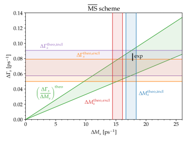
Figure 4: $\Delta\Gamma_{s}$ versus $\Delta M_{s}$. The $|V_{cb}|$ controversy (red vs. blue vertical and orange vs. purple horizontal strips) prevents any conclusion on possible new physics in $\Delta M_{s}$. A combined analysis of $\Delta M_{s}$ and $\Delta\Gamma_{s}$ adds important information, because the SM prediction of $\Delta\Gamma_{s}/\Delta M_{s}$ (green wedge) is independent of $|V_{cb}|$.

In Fig. 4 we confront our predictions for the ratio $\Delta\Gamma_{s}/\Delta M_{s}$ in the $\overline{\rm MS}$ scheme (green band) with the individual predictions of $\Delta\Gamma_{s}$ and $\Delta M_{s}$. The latter are dominated by the uncertainty in the CKM matrix element $V_{ts}$ which is obtained from $V_{cb}$ through CKM unitarity and cancels in the ratio. Fig. 4 illustrates this feature with $|V_{cb}^{\rm incl}|=42.16(51)10^{-3}$ from Bordone et al. (2021) and $|V_{cb}^{\rm excl}|=39.36(68)10^{-3}$ from Aoki et al. (2021). The current experimental results for $\Delta\Gamma_{s}$ and $\Delta M_{s}$ are indicated by the black bar. Once the prediction of $\Delta\Gamma_{s}/\Delta M_{s}$ is improved further, it will be possible to test the SM without CKM uncertainty, and with progress on $|V_{cb}|$ one will be able to constrain new physics in $\Delta M_{s}$ and $\Delta\Gamma_{s}$ individually.

Conclusions. The SM prediction of $\Delta\Gamma_{s}/\Delta M_{s}$ based on the long-standing NLO calculation has two sources of uncertainty which exceed the experimental error: the hadronic matrix elements of the power-suppressed operators and the perturbative coefficients, as inferred from the scale and scheme dependences of the calculated result. With the NNLO calculation presented here we have brought the latter uncertainty to the level of the accuracy of the experimental result. For this we had to calculate 20,000 three-loop diagrams and to solve subtle problems related to the interplay of infrared divergences and evanescent oprators. We have pointed out that $\Delta\Gamma_{s}$ adds information to the usual study of $\Delta M_{s}$, because both quantities probe different new-physics scenarios and $|V_{cb}|$ drops out in the ratio $\Delta\Gamma_{s}/\Delta M_{s}$.

Acknowledgements. We thank Artyom Hovhannisyan and Matthew Wingate for useful discussions and we are grateful to Erik Panzer and Oliver Schnetz for helpful advice regarding the calculation of the master integrals and the simplification of the obtained results with HyperInt and HyperLogProcedures. VS thanks David Broadhurst for enlightening discussions on iterated integrals. This research was supported by the Deutsche Forschungsgemeinschaft (DFG, German Research Foundation) under grant 396021762 — TRR 257 “Particle Physics Phenomenology after the Higgs Discovery”. The Feynman diagrams were drawn with the help of Axodraw Vermaseren (1994) and JaxoDraw Binosi and Theussl (2004).

References

- Elor et al. (2019) Gilly Elor, Miguel Escudero, and Ann Nelson, “Baryogenesis and Dark Matter from Mesons,” Phys. Rev. D 99, 035031 (2019), arXiv:1810.00880 [hep-ph] .
- Alonso-Álvarez et al. (2021) Gonzalo Alonso-Álvarez, Gilly Elor, and Miguel Escudero, “Collider signals of baryogenesis and dark matter from B mesons: A roadmap to discovery,” Phys. Rev. D 104, 035028 (2021), arXiv:2101.02706 [hep-ph] .
- Aaij et al. (2019) Roel Aaij et al. (LHCb), “Updated measurement of time-dependent \it CP-violating observables in decays,” Eur. Phys. J. C 79, 706 (2019), [Erratum: Eur.Phys.J.C 80, 601 (2020)], arXiv:1906.08356 [hep-ex] .
- Sirunyan et al. (2021) Albert M Sirunyan et al. (CMS), “Measurement of the -violating phase in the B J(1020) K+K- channel in proton-proton collisions at 13 TeV,” Phys. Lett. B 816, 136188 (2021), arXiv:2007.02434 [hep-ex] .
- Aad et al. (2021) Georges Aad et al. (ATLAS), “Measurement of the -violating phase in decays in ATLAS at 13 TeV,” Eur. Phys. J. C 81, 342 (2021), arXiv:2001.07115 [hep-ex] .
- Aaltonen et al. (2012) T. Aaltonen et al. (CDF), “Measurement of the Bottom-Strange Meson Mixing Phase in the Full CDF Data Set,” Phys. Rev. Lett. 109, 171802 (2012), arXiv:1208.2967 [hep-ex] .
- Abazov et al. (2012) Victor Mukhamedovich Abazov et al. (D0), “Measurement of the CP-violating phase using the flavor-tagged decay in 8 fb-1 of collisions,” Phys. Rev. D 85, 032006 (2012), arXiv:1109.3166 [hep-ex] .
- (8) Heavy Flavor Averaging Group (HFLAV), “online update at,” https://hflav-eos.web.cern.ch/hflav-eos/osc/PDG_2020/#DMS .
- Gilman and Wise (1979) Frederick J. Gilman and Mark B. Wise, “Effective Hamiltonian for Delta s = 1 Weak Nonleptonic Decays in the Six Quark Model,” Phys. Rev. D 20, 2392 (1979).
- Buras and Weisz (1990) Andrzej J. Buras and Peter H. Weisz, “QCD Nonleading Corrections to Weak Decays in Dimensional Regularization and ’t Hooft-Veltman Schemes,” Nucl. Phys. B 333, 66–99 (1990).
- Buras et al. (1990) Andrzej J. Buras, Matthias Jamin, and Peter H. Weisz, “Leading and Next-to-leading QCD Corrections to Parameter and Mixing in the Presence of a Heavy Top Quark,” Nucl. Phys. B 347, 491–536 (1990).
- Buras et al. (1992) Andrzej J. Buras, Matthias Jamin, M. E. Lautenbacher, and Peter H. Weisz, “Effective Hamiltonians for and nonleptonic decays beyond the leading logarithmic approximation,” Nucl. Phys. B 370, 69–104 (1992), [Addendum: Nucl.Phys.B 375, 501 (1992)].
- Gorbahn and Haisch (2005) Martin Gorbahn and Ulrich Haisch, “Effective Hamiltonian for non-leptonic decays at NNLO in QCD,” Nucl. Phys. B 713, 291–332 (2005), arXiv:hep-ph/0411071 .
- Gambino et al. (2003) Paolo Gambino, Martin Gorbahn, and Ulrich Haisch, “Anomalous dimension matrix for radiative and rare semileptonic B decays up to three loops,” Nucl. Phys. B 673, 238–262 (2003), arXiv:hep-ph/0306079 .
- Gorbahn et al. (2005) Martin Gorbahn, Ulrich Haisch, and Mikolaj Misiak, “Three-loop mixing of dipole operators,” Phys. Rev. Lett. 95, 102004 (2005), arXiv:hep-ph/0504194 .
- Khoze and Shifman (1983) Valery A. Khoze and Mikhail A. Shifman, “HEAVY QUARKS,” Sov. Phys. Usp. 26, 387 (1983).
- Shifman and Voloshin (1985) Mikhail A. Shifman and M. B. Voloshin, “Preasymptotic Effects in Inclusive Weak Decays of Charmed Particles,” Sov. J. Nucl. Phys. 41, 120 (1985).
- Khoze et al. (1987) Valery A. Khoze, Mikhail A. Shifman, N. G. Uraltsev, and M. B. Voloshin, “On Inclusive Hadronic Widths of Beautiful Particles,” Sov. J. Nucl. Phys. 46, 112 (1987).
- Chay et al. (1990) Junegone Chay, Howard Georgi, and Benjamin Grinstein, “Lepton energy distributions in heavy meson decays from QCD,” Phys. Lett. B 247, 399–405 (1990).
- Bigi and Uraltsev (1992) Ikaros I. Y. Bigi and N. G. Uraltsev, “Gluonic enhancements in non-spectator beauty decays: An Inclusive mirage though an exclusive possibility,” Phys. Lett. B 280, 271–280 (1992).
- Bigi et al. (1992) Ikaros I. Y. Bigi, N. G. Uraltsev, and A. I. Vainshtein, “Nonperturbative corrections to inclusive beauty and charm decays: QCD versus phenomenological models,” Phys. Lett. B 293, 430–436 (1992), [Erratum: Phys.Lett.B 297, 477–477 (1992)], arXiv:hep-ph/9207214 .
- Bigi et al. (1993) Ikaros I. Y. Bigi, Mikhail A. Shifman, N. G. Uraltsev, and Arkady I. Vainshtein, “QCD predictions for lepton spectra in inclusive heavy flavor decays,” Phys. Rev. Lett. 71, 496–499 (1993), arXiv:hep-ph/9304225 .
- Blok et al. (1994) B. Blok, L. Koyrakh, Mikhail A. Shifman, and A. I. Vainshtein, “Differential distributions in semileptonic decays of the heavy flavors in QCD,” Phys. Rev. D 49, 3356 (1994), [Erratum: Phys.Rev.D 50, 3572 (1994)], arXiv:hep-ph/9307247 .
- Manohar and Wise (1994) Aneesh V. Manohar and Mark B. Wise, “Inclusive semileptonic B and polarized Lambda(b) decays from QCD,” Phys. Rev. D 49, 1310–1329 (1994), arXiv:hep-ph/9308246 .
- Lenz (2015) Alexander Lenz, “Lifetimes and heavy quark expansion,” Int. J. Mod. Phys. A 30, 1543005 (2015), arXiv:1405.3601 [hep-ph] .
- Beneke et al. (1999) M. Beneke, G. Buchalla, C. Greub, A. Lenz, and U. Nierste, “Next-to-leading order QCD corrections to the lifetime difference of B(s) mesons,” Phys. Lett. B 459, 631–640 (1999), arXiv:hep-ph/9808385 .
- Ciuchini et al. (2003) M. Ciuchini, E. Franco, V. Lubicz, F. Mescia, and C. Tarantino, “Lifetime differences and CP violation parameters of neutral B mesons at the next-to-leading order in QCD,” JHEP 08, 031 (2003), arXiv:hep-ph/0308029 .
- Beneke et al. (2003) Martin Beneke, Gerhard Buchalla, Alexander Lenz, and Ulrich Nierste, “CP asymmetry in flavor specific B decays beyond leading logarithms,” Phys. Lett. B 576, 173–183 (2003), arXiv:hep-ph/0307344 .
- Lenz and Nierste (2007) Alexander Lenz and Ulrich Nierste, “Theoretical update of mixing,” JHEP 06, 072 (2007), arXiv:hep-ph/0612167 .
- Asatrian et al. (2017) H. M. Asatrian, Artyom Hovhannisyan, Ulrich Nierste, and Arsen Yeghiazaryan, “Towards next-to-next-to-leading-log accuracy for the width difference in the system: fermionic contributions to order and ,” JHEP 10, 191 (2017), arXiv:1709.02160 [hep-ph] .
- Asatrian et al. (2020) Hrachia M. Asatrian, Hrachya H. Asatryan, Artyom Hovhannisyan, Ulrich Nierste, Sergey Tumasyan, and Arsen Yeghiazaryan, “Penguin contribution to the width difference and asymmetry in - mixing at order ,” Phys. Rev. D 102, 033007 (2020), arXiv:2006.13227 [hep-ph] .
- Hovhannisyan and Nierste (2022) Artyom Hovhannisyan and Ulrich Nierste, “Addendum to: Towards next-to-next-to-leading-log accuracy for the width difference in the system: fermionic contributions to order and ,” (2022), arXiv:2204.11907 [hep-ph] .
- Gerlach et al. (2021) Marvin Gerlach, Ulrich Nierste, Vladyslav Shtabovenko, and Matthias Steinhauser, “Two-loop QCD penguin contribution to the width difference in Bs mixing,” JHEP 07, 043 (2021), arXiv:2106.05979 [hep-ph] .
- Gerlach et al. (2022a) Marvin Gerlach, Ulrich Nierste, Vladyslav Shtabovenko, and Matthias Steinhauser, “The width difference in mixing at order and beyond,” JHEP 04, 006 (2022a), arXiv:2202.12305 [hep-ph] .
- Dowdall et al. (2019) R. J. Dowdall, C. T. H. Davies, R. R. Horgan, G. P. Lepage, C. J. Monahan, J. Shigemitsu, and M. Wingate, “Neutral B-meson mixing from full lattice QCD at the physical point,” Phys. Rev. D 100, 094508 (2019), arXiv:1907.01025 [hep-lat] .
- Kirk et al. (2017) M. Kirk, A. Lenz, and T. Rauh, “Dimension-six matrix elements for meson mixing and lifetimes from sum rules,” JHEP 12, 068 (2017), [Erratum: JHEP 06, 162 (2020)], arXiv:1711.02100 [hep-ph] .
- King et al. (2021) Daniel King, Alexander Lenz, and Thomas Rauh, “ breaking effects in and meson lifetimes,” (2021), arXiv:2112.03691 [hep-ph] .
- Beneke et al. (1996) M. Beneke, G. Buchalla, and I. Dunietz, “Width Difference in the System,” Phys. Rev. D 54, 4419–4431 (1996), [Erratum: Phys.Rev.D 83, 119902 (2011)], arXiv:hep-ph/9605259 .
- Davies et al. (2020) Christine T. H. Davies, Judd Harrison, G. Peter Lepage, Christopher J. Monahan, Junko Shigemitsu, and Matthew Wingate (HPQCD), “Lattice QCD matrix elements for the width difference beyond leading order,” Phys. Rev. Lett. 124, 082001 (2020), arXiv:1910.00970 [hep-lat] .
- Chetyrkin et al. (1998a) Konstantin G. Chetyrkin, Mikolaj Misiak, and Manfred Munz, “ nonleptonic effective Hamiltonian in a simpler scheme,” Nucl. Phys. B 520, 279–297 (1998a), arXiv:hep-ph/9711280 .
- Nogueira (1993) Paulo Nogueira, “Automatic Feynman graph generation,” J. Comput. Phys. 105, 279–289 (1993).
- Gerlach et al. (2022b) Marvin Gerlach, Florian Herren, and Martin Lang, “tapir: A tool for topologies, amplitudes, partial fraction decomposition and input for reductions,” (2022b), arXiv:2201.05618 [hep-ph] .
- Harlander et al. (1998) R. Harlander, T. Seidensticker, and M. Steinhauser, “Complete corrections of Order alpha alpha-s to the decay of the Z boson into bottom quarks,” Phys. Lett. B 426, 125–132 (1998), arXiv:hep-ph/9712228 .
- Seidensticker (1999) T. Seidensticker, “Automatic application of successive asymptotic expansions of Feynman diagrams,” in 6th International Workshop on New Computing Techniques in Physics Research: Software Engineering, Artificial Intelligence Neural Nets, Genetic Algorithms, Symbolic Algebra, Automatic Calculation (1999) arXiv:hep-ph/9905298 .
- Smirnov and Chuharev (2020) A. V. Smirnov and F. S. Chuharev, “FIRE6: Feynman Integral REduction with Modular Arithmetic,” Comput. Phys. Commun. 247Â , 106877 (2020), arXiv:1901.07808 [hep-ph] .
- Lee (2012) R. N. Lee, “Presenting LiteRed: a tool for the Loop InTEgrals REDuction,” (2012), arXiv:1212.2685 [hep-ph] .
- Lee (2014) Roman N. Lee, “LiteRed 1.4: a powerful tool for reduction of multiloop integrals,” J. Phys. Conf. Ser. 523, 012059 (2014), arXiv:1310.1145 [hep-ph] .
- Mertig et al. (1991) R. Mertig, M. Bohm, and Ansgar Denner, “FEYN CALC: Computer algebraic calculation of Feynman amplitudes,” Comput. Phys. Commun. 64, 345–359 (1991).
- Shtabovenko et al. (2016) Vladyslav Shtabovenko, Rolf Mertig, and Frederik Orellana, “New Developments in FeynCalc 9.0,” Comput. Phys. Commun. 207, 432–444 (2016), arXiv:1601.01167 [hep-ph] .
- Shtabovenko et al. (2020) Vladyslav Shtabovenko, Rolf Mertig, and Frederik Orellana, “FeynCalc 9.3: New features and improvements,” Comput. Phys. Commun. 256, 107478 (2020), arXiv:2001.04407 [hep-ph] .
- Shtabovenko (2021) Vladyslav Shtabovenko, “FeynCalc goes multiloop,” in 20th International Workshop on Advanced Computing and Analysis Techniques in Physics Research: AI Decoded - Towards Sustainable, Diverse, Performant and Effective Scientific Computing (2021) arXiv:2112.14132 [hep-ph] .
- Panzer (2015) Erik Panzer, Feynman integrals and hyperlogarithms, Ph.D. thesis, Humboldt U. (2015), arXiv:1506.07243 [math-ph] .
- Duhr and Dulat (2019) Claude Duhr and Falko Dulat, “PolyLogTools — polylogs for the masses,” JHEP 08, 135 (2019), arXiv:1904.07279 [hep-th] .
- (54) Oliver Schnetz, “HyperLogProcedures,” https://www.math.fau.de/person/oliver-schnetz .
- Chetyrkin et al. (1998b) Konstantin G. Chetyrkin, Mikolaj Misiak, and Manfred Munz, “Beta functions and anomalous dimensions up to three loops,” Nucl. Phys. B 518, 473–494 (1998b), arXiv:hep-ph/9711266 .
- Ciuchini et al. (2002) Marco Ciuchini, E. Franco, V. Lubicz, and F. Mescia, “Next-to-leading order QCD corrections to spectator effects in lifetimes of beauty hadrons,” Nucl. Phys. B 625, 211–238 (2002), arXiv:hep-ph/0110375 .
- Herren and Steinhauser (2018) Florian Herren and Matthias Steinhauser, “Version 3 of RunDec and CRunDec,” Comput. Phys. Commun. 224, 333–345 (2018), arXiv:1703.03751 [hep-ph] .
- Zyla et al. (2020) P. A. Zyla et al. (Particle Data Group), “Review of Particle Physics,” PTEP 2020, 083C01 (2020).
- Chetyrkin et al. (2017) Konstantin G. Chetyrkin, Johann H. Kuhn, Andreas Maier, Philipp Maierhofer, Peter Marquard, Matthias Steinhauser, and Christian Sturm, “Addendum to “Charm and bottom quark masses: An update”,” (2017), 10.1103/PhysRevD.96.116007, [Addendum: Phys.Rev.D 96, 116007 (2017)], arXiv:1710.04249 [hep-ph] .
- Bazavov et al. (2018) A. Bazavov et al., “- and -meson leptonic decay constants from four-flavor lattice QCD,” Phys. Rev. D 98, 074512 (2018), arXiv:1712.09262 [hep-lat] .
- Beneke (1998) M. Beneke, “A Quark mass definition adequate for threshold problems,” Phys. Lett. B 434, 115–125 (1998), arXiv:hep-ph/9804241 .
- Bigi et al. (1994) Ikaros I. Y. Bigi, Mikhail A. Shifman, N. G. Uraltsev, and A. I. Vainshtein, “The Pole mass of the heavy quark. Perturbation theory and beyond,” Phys. Rev. D 50, 2234–2246 (1994), arXiv:hep-ph/9402360 .
- Beneke and Braun (1994) M. Beneke and Vladimir M. Braun, “Heavy quark effective theory beyond perturbation theory: Renormalons, the pole mass and the residual mass term,” Nucl. Phys. B 426, 301–343 (1994), arXiv:hep-ph/9402364 .
- Beneke (2021) Martin Beneke, “Pole mass renormalon and its ramifications,” Eur. Phys. J. ST 230, 2565–2579 (2021), arXiv:2108.04861 [hep-ph] .
- Aaij et al. (2022) R. Aaij et al. (LHCb), “Precise determination of the – oscillation frequency,” Nature Phys. 18, 1–5 (2022), arXiv:2104.04421 [hep-ex] .
- (66) Marvin Gerlach, Ulrich Nierste, Vladyslav Shtabovenko, and Matthias Steinhauser, “Next-to-next-to-leading order QCD corrections to the -meson mixing,” in preparation .
- Bordone et al. (2021) Marzia Bordone, Bernat Capdevila, and Paolo Gambino, “Three loop calculations and inclusive Vcb,” Phys. Lett. B 822, 136679 (2021), arXiv:2107.00604 [hep-ph] .
- Aoki et al. (2021) Y. Aoki et al., “FLAG Review 2021,” (2021), arXiv:2111.09849 [hep-lat] .
- Vermaseren (1994) J. A. M. Vermaseren, “Axodraw,” Comput. Phys. Commun. 83, 45–58 (1994).
- Binosi and Theussl (2004) D. Binosi and L. Theussl, “JaxoDraw: A Graphical user interface for drawing Feynman diagrams,” Comput. Phys. Commun. 161, 76–86 (2004), arXiv:hep-ph/0309015 .