Islands for Entanglement Negativity in Communicating Black Holes

Abstract

We obtain the holographic entanglement negativity for bipartite mixed states at a finite temperature in baths described by conformal field theories dual to configurations involving two communicating black holes in a braneworld geometry. In this context, we analyze the mixed state entanglement structure characterized by the information transfer between the black holes. The model corresponds to a configuration of two dimensional eternal JT black holes in a braneworld geometry involving two Planck branes coupled through shared bath systems described by $CFT_{2}$s. Our results reproduce analogue of the Page curves for the entanglement negativity obtained earlier in the context of random matrix theory and from geometric evaporation in JT black hole configurations.

1 Introduction

Over the last few decades, the black hole information loss paradox Hawking:1975vcx ; Hawking:1976ra has been one of the most engaging and fascinating issues in the quest for a quantum theory of gravity. The central element of this puzzle involves the monotonic increase in the entanglement entropy of the Hawking radiation from an evaporating black hole resulting in the fine grained entropy to dominate the coarse grained entropy at late times which leads to a violation of unitarity. It could be shown that the unitarity of the black hole evaporation process required the corresponding entanglement entropy of the Hawking radiation to follow a Page curve Page:1993wv . Very recently this issue has been addressed through the fascinating development of the island proposal which has led to the exciting possibility of a resolution of this long standing paradox Engelhardt:2014gca ; Almheiri:2019psf ; Penington:2019npb ; Almheiri:2019hni ; Almheiri:2020cfm ; Almheiri:2019yqk ; Penington:2019kki ; Almheiri:2019qdq . The island or the quantum extremal surface (QES) formula for entanglement entropy was motivated from the quantum corrected Ryu-Takayanagi (RT) proposal Ryu:2006bv ; Ryu:2006ef ; Hubeny:2007xt ; Faulkner:2013ana and this may be obtained by extremizing the generalized fine-grained entanglement entropy of the Hawking radiation. In this context it could be shown that at late times the entanglement entropy of a bath subsystem in the radiation flux of the black hole receives contributions from a region in the black hole geometry termed the entanglement island. Specifically the bath subsystem and the island regions were shown to be a part of the same entanglement wedge in higher dimension as described in Almheiri:2019hni . The corresponding island formula for the generalized fine-grained entropy of a subsystem $\mathcal{R}$ in the radiation bath is given as,

$$S[\mathcal{R}]=\min\left\{\operatorname{ext}_{Is(\mathcal{R})}\left[\frac{\operatorname{Area}[\partial Is(\mathcal{R})]}{4G_{N}}+S_{eff}[\operatorname{\mathcal{R}}\cup Is(\mathcal{R})]\right]\right\},$$ (1)

where $Is(\mathcal{R})$ is the island region in the black hole geometry corresponding to the subsystem $\mathcal{R}$ in the radiation bath .

From the perspective described above, an extremely interesting and elegant model has been proposed in Balasubramanian:2021xcm similar to the one described in Almheiri:2020cfm . However the authors of Balasubramanian:2021xcm considered two copies of finite sized reservoirs described by $CFT_{2}$s each with two quantum dots located at their boundaries at a finite temperature. The holographic dual of these quantum dots are described by Planck branes in the bulk $AdS_{3}$ space time which supports $AdS_{2}$ geometries with Jackiw-Teitelboim (JT) gravity Teitelboim:1983ux ; Jackiw:1984je . Hence the two Planck branes may involve eternal JT black holes which communicate with each other through the common radiation reservoirs. Note that from the perspective of each brane, the bath together with the other Planck brane appears as a gravitating configuration Balasubramanian:2021xcm . For this configuration, the authors of Balasubramanian:2021xcm have computed the generalized entanglement entropy for a finite subsystem in the radiation reservoirs which once again characterizes the communication between the two eternal JT black holes on the Planck branes.

In a separate context, it is well known in quantum information theory that the entanglement entropy is an appropriate measure for the characterization of pure state entanglement, however for mixed states it receives contributions from irrelevant classical and quantum correlations. A consistent and computable measure for the characterization of mixed state entanglement which serves as an upper bound to the distillable entanglement is described by the entanglement negativity introduced in Vidal:2002zz ; PhysRevLett.95.090503 . In Calabrese:2014yza ; Calabrese:2012nk ; Calabrese:2012ew the authors established a replica technique to compute the entanglement negativity for bipartite pure and mixed states in $CFT_{2}$. The first holographic computation for the entanglement negativity for the pure vacuum state in $CFT$s was described in Rangamani:2014ywa . Subsequently general holographic proposals for the entanglement negativity of bipartite pure and mixed states in $CFT_{2}$s involving specific algebraic sums of the lengths of geodesics homologous to various combinations of subsystems were introduced in Chaturvedi:2016rcn ; Jain:2017aqk ; Malvimat:2018txq . It is interesting to note that the authors of Kudler-Flam:2018qjo had proposed an alternative prescription for the holographic entanglement negativity of bipartite mixed states in $CFT$s in terms of the backreacted minimal entanglement wedge cross section (EWCS) in the context of the $AdS/CFT$ scenario, further refined in KumarBasak:2020eia . For spherically entangling surfaces of the subsystems considered in the dual $CFT$s, the backreaction parameter was described by an overall numerical factor which is dependent on the dimension of the $CFT$s. A proof for this duality between the holographic entanglement negativity and the bulk EWCS was further established in Kusuki:2019zsp involving the idea of reflected entropy described in Dutta:2019gen .

A generalization of these proposals for the entanglement negativity in $CFT_{2}$s coupled to semiclassical gravity was advanced in KumarBasak:2020ams with a possible derivation using the replica wormhole contributions to the gravitational path integral involving replica symmetry breaking saddles as discussed in Dong:2021clv . In the present article, we focus on the computation of the holographic entanglement negativity for various bipartite mixed states in a braneworld model Balasubramanian:2021xcm mentioned earlier. We consider different scenarios involving the subsystem sizes and the time for two adjacent and disjoint subsystems located in the bath regions at a finite temperature. Furthermore, we discuss the behaviours of the entanglement negativity profiles obtained in these scenarios in terms of the Hawking radiation. We observe interesting similarities between our results with those described in KumarBasak:2021rrx ; Shapourian:2020mkc .

In the appendix A, we explore a similar model of communicating black holes described extensively in Geng:2021iyq where the authors have considered a $BCFT_{2}$ on a manifold with two boundaries in the context of the $AdS_{3}/BCFT_{2}$ scenario. The holographic dual of this configuration is described by a wedge enclosed within the two KR branes in the bulk $AdS_{3}$ braneworld geometry. The KR branes involve $CFT_{2}$ matter fields with a constant Lagrangian which is connected to the $CFT_{2}$ on the asymptotic boundary of the dual $AdS_{3}$ geometry through transparent boundary conditions Almheiri:2019yqk ; Almheiri:2019hni . At a finite temperature, black holes may be induced on these two KR branes from the higher dimensional eternal $AdS_{3}$ BTZ black hole. In this model, we compute the holographic entanglement negativity and obtain the corresponding Page curves for various bipartite mixed states of two adjacent and disjoint subsystems in the bath $BCFT_{2}$s at a finite temperature.

This article is organized as follows. In section 2, we review the relevant works discussed in the braneworld model Balasubramanian:2021xcm and holographic entanglement negativity described in Jain:2017aqk ; Malvimat:2018txq . Next in section 3, we apply the results for the generalized entanglement entropy discussed in section 2 for different cases of adjacent and disjoint subsystems and obtain the corresponding holographic entanglement negativity. In appendix A, we first compute the entanglement entropy for a generic subsystem in the context of another model of braneworld geometry Geng:2021iyq . Subsequently, we apply these results to further compute the holographic entanglement negativity for various bipartite mixed states using the holographic proposals described in section 2. In appendix B, we list the results for the holographic entanglement negativity for all the different scenarios discussed in section 3. Finally in the section 4, we summarize and discuss our results and future open issues.

2 Review of earlier results

2.1 Braneworld model

In this subsection we will be reviewing an intriguing model of finite sized non-gravitating reservoirs, coupled with two quantum dots at its two boundaries Balasubramanian:2021xcm . The holographic dual of these quantum dots are Plank branes described by $AdS_{2}$ geometries. The maximal extension of the Penrose diagram in this context consists of two eternal JT black holes in the $AdS_{2}$ space time located on the Planck branes. In this case the usual reflecting boundaries are coupled to two non-gravitating reservoirs through transparent boundary conditions Almheiri:2019yqk ; Almheiri:2019qdq such that the two black holes are connected to each other through the shared reservoirs. This construction involves identical matter $CFT_{2}$s on both the reservoirs and the gravity regions. Interestingly, a single brane together with a reservoir appears to be a gravitating one from the perspective of each brane. In this framework, the authors of Balasubramanian:2021xcm have considered the two black holes at different temperatures and obtained the generalized entanglement entropy of a finite region in the two reservoirs by utilizing eq. 1. The first term corresponds to the value of the dilaton field in the JT gravity with a constant $\phi_{0}$ added to it whereas the second term follows from the usual computation of the entanglement entropy Ryu:2006bv of a segment $\mathcal{R}\cup Is(\mathcal{R})$. The generalized entanglement entropy of the finite region in the reservoirs characterizes the communication between the two JT black holes on the Planck branes. In what follows we review the computation of the generalized entanglement entropy for a subsystem in the radiation reservoirs while considering the JT black holes on the Planck branes at a same temperature.

2.1.1 Entanglement entropy in the two black hole configuration

In this subsection, we consider two eternal JT black holes at the same temperature and describe the explicit computation for the generalized entanglement entropy for a subsystem $A$ consisting of the union of two identical line segments in the two copies of the reservoirs.

For this configuration, the metrics referring to the exterior regions of the two eternal JT black holes may be written as

$$ds_{1}^{2} = \frac{4\pi^{2}}{\beta^{2}}\frac{-dt^{2}+d\xi^{2}}{\sinh^{2}\frac{2\pi\xi}{\beta}},\quad\xi\in\left(-\infty,-\epsilon\right]\,,$$ (2)

$$ds_{2}^{2} = \frac{4\pi^{2}}{\beta^{2}}\frac{-dt^{2}+d\xi^{2}}{\sinh^{2}\frac{2\pi}{\beta}(\xi-L)},\quad\xi\in\left[L+\epsilon,+\infty\right)\,,$$ (3)

where $L$ is the length of each radiation reservoir with a metric defined by

$$ds_{R}^{2}=\frac{-dt^{2}+d\xi^{2}}{\epsilon^{2}}\,,\quad\xi\in\left[-\epsilon,L+\epsilon\right]\,$$ (4)

where the reservoir is glued continuously to the surfaces $\xi=-\epsilon$ and $L+\epsilon$. The dilaton profiles for the two eternal JT black holes on the Planck branes are then given as follows

$$\phi_{a}(\xi) = \frac{2\pi\phi_{r}}{\beta}\coth\frac{2\pi\xi}{\beta}\,,$$ (5)

$$\phi_{b}(\xi) = \frac{2\pi\phi_{r}}{\beta}\coth\frac{2\pi}{\beta}\left(\xi-L\right).$$ (6)

We now compute the generalized entanglement entropy for the subsystem described by the union of two identical segments $A=[p_{1},p_{2}]\cup[p_{3},p_{4}]$ in the radiation regions of the two TFD copies. The end points of the two corresponding segments in the ($\xi,t$) coordinates are specified as follows Balasubramanian:2021xcm

$$p_{1}=(v,-t+i\frac{\beta}{2}),\quad p_{2}=(u,-t+i\frac{\beta}{2}),\quad p_{3}=(u,t),\quad p_{4}=(v,t)\,.$$ (7)

In this case there are seven possible contributions to the corresponding entanglement entropy due to the different structures of the RT surfaces supported by the subsystems mentioned above. In what follows, we describe these distinct contributions in detail.

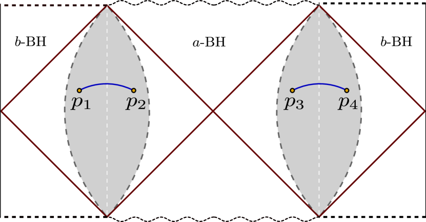
(a)

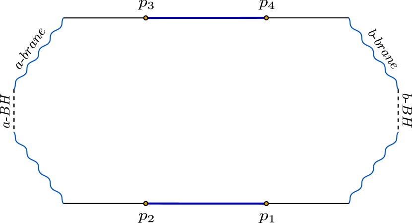
(b)

Figure 1: (a) The maximal extension of the Penrose diagram for two $AdS_{2}$ eternal black holes. A subsystem given by the union of two segments is considered in the radiation reservoirs (shaded regions) with end points $p_{1}$, $p_{2}$, $p_{3}$, $p_{4}$. Note that the left and the right most black lines are identified in this diagram. (b) A constant time slice of the $AdS_{2}$ eternal black holes where the Planck branes are denoted by the wigly lines and the black hole intereiors are shown by the dotted lines. (Figures modified from Balasubramanian:2021xcm ; Geng:2021hlu )

$\bm{(a)}$ We first discuss the configuration which is completely connected and does not include any island region in the gravity sector. The end points of the two segments of the subsystem $A$ are connected to each other $p_{1}\leftrightarrow p_{4}$ and $p_{2}\leftrightarrow p_{3}$ by two geodesics in the 3-dimensional bulk as depicted in fig. 3(a). We term these geodesics as bulk-type RT surfaces. The expression for the corresponding generalized entanglement entropy may be obtained utilizing eq. 1 as follows

$$\mathcal{S}_{A}^{\text{bulk}}=2\frac{c}{3}\log\left[\frac{\beta}{\pi}\cosh\frac{2\pi t}{\beta}\right].$$ (8)

$\bm{(b)}$ The second configuration also corresponds to a fully connected one which includes island regions from both the JT black holes. We may obtain the generalized entanglement entropy for the subsystem $A$ following a procedure analogous to the single black hole case as discussed in Balasubramanian:2021xcm . However for this configuration, the computation involves an extremization of eq. 1 over two island regions located on the $a$ and the $b$-black holes. The subsystem $A$ in this context admits RT surfaces which start from $\partial A$ and intersect the exterior regions of both the black holes. We call these RT surfaces $ab$-type which are depicted in fig. 3(b). The corresponding generalized entanglement entropy for the subsystem $A$ may then be expressed as

$$\mathcal{S}_{A}^{ab} = 4\phi_{0}+\frac{4\pi\phi_{r}}{\beta}\coth\left(\frac{2\pi}{\beta}u+\log\frac{24\pi\phi}{c\beta}\right)+\frac{c}{3}\log\left[\frac{\beta}{\pi}\;\frac{\cosh\left(\frac{4\pi}{\beta}u+\log\frac{24\pi\phi}{c\beta}\right)-1}{\sinh\left(\frac{2\pi}{\beta}u+\log\frac{24\pi\phi}{c\beta}\right)}\right]$$

$$+ \frac{4\pi\phi_{r}}{\beta}\coth\left(\frac{2\pi}{\beta}(L-v)+\log\frac{24\pi\phi}{c\beta}\right)+\frac{c}{3}\log\left[\frac{\beta}{\pi}\;\frac{\cosh\left(\frac{4\pi}{\beta}(L-v)+\log\frac{24\pi\phi}{c\beta}\right)-1}{\sinh\left(\frac{2\pi}{\beta}(L-v)+\log\frac{24\pi\phi}{c\beta}\right)}\right].$$

$\bm{(c)}$ We now discuss a disconnected configuration which does not include any island region as shown in fig. 3(c). Here the entanglement entropy for the subsystem $A$ may be obtained from the geodesics which are homologous to each of the segments in the two TFD copies separately. We term these geodesics as dome-type RT surfaces. The corresponding generalized entanglement entropy for this configuration is given by the following expression

$$\mathcal{S}_{A}^{\text{dome}}=2\frac{c}{3}\log\left(\frac{\beta}{\pi}\sinh\frac{\pi}{\beta}|u-v|\right).$$ (10)

$\bm{(d)}$ This configuration includes an island region in the $a$-black hole corresponding to two geodesics which start from the end points $p_{2}$, $p_{3}$ of each of the segments and intersect the two exterior regions of the $a$-black hole. However, the other end points of the subsystem $A$ are connected to each other $p_{4}\leftrightarrow p_{1}$ by another geodesic. In this connected configuration, we term the corresponding geodesics as $a$-bulk type RT surfaces which are depicted in fig. 3(d). The expression for the generalized entanglement entropy for the subsystem $A$ may be computed using eq. 1 as follows

$$\mathcal{S}_{A}^{a\text{-bulk}} = 4\phi_{0}+\frac{4\pi\phi_{r}}{\beta}\coth\left(\frac{2\pi}{\beta}u+\log\frac{24\pi\phi}{c\beta}\right)$$ (11)

$$+ \frac{c}{3}\log\left[\frac{\beta}{\pi}\;\frac{\cosh\left(\frac{4\pi}{\beta}u+\log\frac{24\pi\phi}{c\beta}\right)-1}{\sinh\left(\frac{2\pi}{\beta}u+\log\frac{24\pi\phi}{c\beta}\right)}\right]+\frac{c}{3}\log\left[\frac{\beta}{\pi}\cosh\frac{2\pi t}{\beta}\right].$$

$\bm{(e)}$ Similar to the previous case, we now discuss another connected configuration which admits an island region in the $b$-black hole geometry only. The geodesics in this case start from the end points $p_{1}$, $p_{4}$ of the two segments and intersect the two exterior regions of the $b$-black hole. However another geodesic connects the other end points $p_{2}$, $p_{3}$ of the subsystem $A$. In contrast to the previous case, these geodesics are termed as $b$-bulk type RT surfaces (fig. 3(e)). The corresponding generalized entanglement entropy for the subsystem $A$ in this case may be obtained utilizing eq. 1 as follows

$$\mathcal{S}_{A}^{b\text{-bulk}} = 4\phi_{0}+\frac{4\pi\phi_{r}}{\beta}\coth\left(\frac{2\pi}{\beta}(L-v)+\log\frac{24\pi\phi}{c\beta}\right)$$ (12)

$$+ \frac{c}{3}\log\left[\frac{\beta}{\pi}\;\frac{\cosh\left(\frac{4\pi}{\beta}(L-v)+\log\frac{24\pi\phi}{c\beta}\right)-1}{\sinh\left(\frac{2\pi}{\beta}(L-v)+\log\frac{24\pi\phi}{c\beta}\right)}\right]+\frac{c}{3}\log\left[\frac{\beta}{\pi}\cosh\frac{2\pi t}{\beta}\right].$$

$\bm{(f)}$ Another disconnected configuration includes two island regions in the gravity sector where the corresponding geodesics, which are termed as $aa$-type RT surfaces, start from $\partial A$ and intersect the two exterior regions of the $a$-black hole (fig. 3(f)). The generalized entanglement entropy for this disconnected configuration is computed by extremizing eq. 1 over the two island regions and is given as

$$\mathcal{S}_{A}^{aa} = 4\phi_{0}+\frac{4\pi\phi_{r}}{\beta}\coth\left(\frac{2\pi}{\beta}u+\log\frac{24\pi\phi}{c\beta}\right)+\frac{c}{3}\log\left[\frac{\beta}{\pi}\;\frac{\cosh\left(\frac{4\pi}{\beta}u+\log\frac{24\pi\phi}{c\beta}-1\right)}{\sinh\left(\frac{2\pi}{\beta}u+\log\frac{24\pi\phi}{c\beta}\right)}\right]$$ (13)

$$+ \frac{4\pi\phi_{r}}{\beta}\coth\left(\frac{2\pi}{\beta}v+\log\frac{24\pi\phi}{c\beta}\right)+\frac{c}{3}\log\left[\frac{\beta}{\pi}\;\frac{\cosh\left(\frac{4\pi}{\beta}v+\log\frac{24\pi\phi}{c\beta}-1\right)}{\sinh\left(\frac{2\pi}{\beta}v+\log\frac{24\pi\phi}{c\beta}\right)}\right].$$

$\bm{(g)}$ Finally we consider the last configuration which is similar to the preceding one but with the island regions in the $b$-black hole geometry as shown in fig. 3(g). In this disconnected configuration, the RT surfaces supported by the subsystem $A$ are termed $bb$-type. Once again, the corresponding generalized entanglement entropy may be obtained utilizing eq. 1 as follows

$$\mathcal{S}_{A}^{bb}= \,4\phi_{0}+\frac{4\pi\phi_{r}}{\beta}\coth\left(\frac{2\pi}{\beta}(L-v)+\log\frac{24\pi\phi}{c\beta}\right)$$

$$+ \frac{c}{3}\log\left[\frac{\beta}{\pi}\;\frac{\cosh\left(\frac{4\pi}{\beta}(L-v)+\log\frac{24\pi\phi}{c\beta}\right)-1}{\sinh\left(\frac{2\pi}{\beta}(L-v)+\log\frac{24\pi\phi}{c\beta}\right)}\right]$$

$$+ \frac{4\pi\phi_{r}}{\beta}\coth\left(\frac{2\pi}{\beta}(L-u)+\log\frac{24\pi\phi}{c\beta}\right)+\frac{c}{3}\log\left[\frac{\beta}{\pi}\;\frac{\cosh\left(\frac{4\pi}{\beta}(L-u)+\log\frac{24\pi\phi}{c\beta}\right)-1}{\sinh\left(\frac{2\pi}{\beta}(L-v)+\log\frac{24\pi\phi}{c\beta}\right)}\right].$$

The generalized entanglement entropy for the subsystem $A$ in the radiation reservoirs may now be determined from the minimum of all the above possible contributions as follows

$$S_{A}=\text{min}\left(\mathcal{S}_{A}^{\text{bulk}},\mathcal{S}_{A}^{ab},\mathcal{S}_{A}^{\text{dome}},\mathcal{S}_{A}^{a\text{-bulk}},\mathcal{S}_{A}^{b\text{-bulk}},\mathcal{S}_{A}^{aa},\mathcal{S}_{A}^{bb}\right)\,.$$ (15)

In what follows we plot the generalized entanglement entropies for the subsystem $A$ with respect to the time and its size for all the above possible configurations obtained from the respective structures of the corresponding RT surfaces.

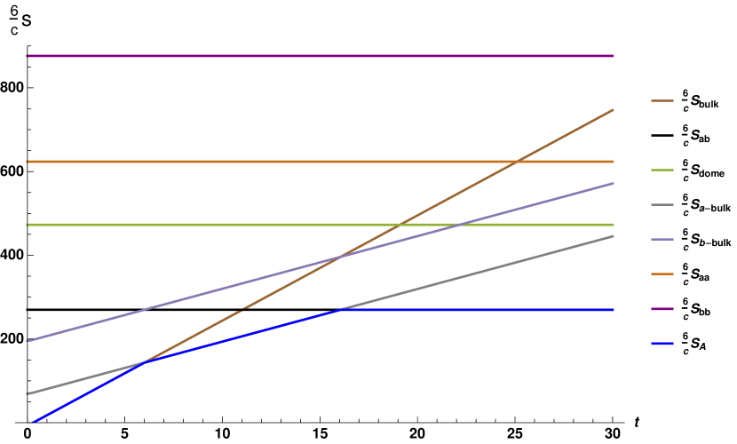
(a) Entanglement entropies corresponding to the different RT surfaces w.r.t time. Here $A=[.02L,.78L]$ and time $t$ is varied from [0, 30].

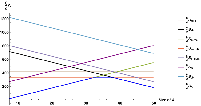
(b) Entanglement entropies corresponding to the different RT surfaces w.r.t the size of the subsystem $A$. Here $t=17$ and the size of $A$ is varied from $[.1L,.99L]$.

Figure 2: In the above figures, we have chosen $\beta=1$, $c=500$, $\phi_{0}=\frac{30c}{6}$, $\phi_{r}=\frac{30}{\pi}$, $L=\frac{16\pi}{\beta}$, $\epsilon=.001$.

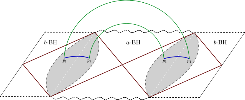
(a)

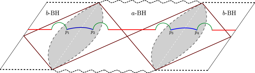
(b)

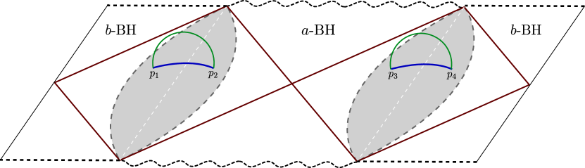
(c)

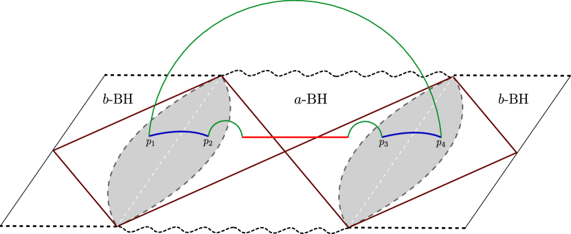
(d)

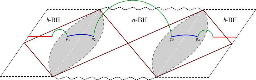
(e)

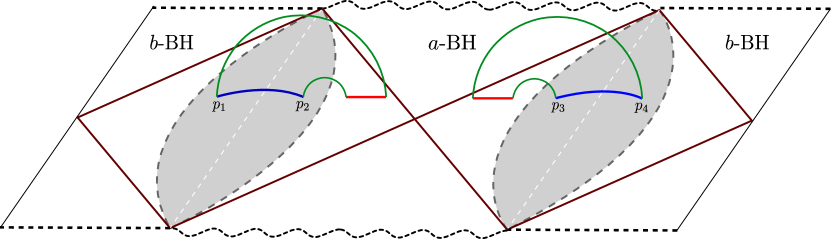
(f)

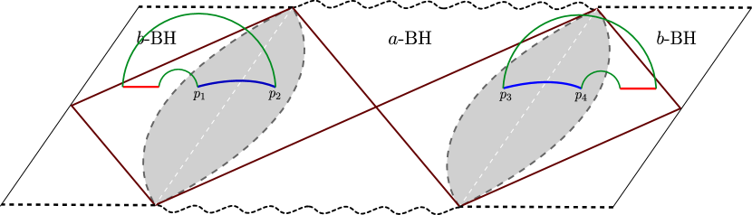
(g)

Figure 3: The schematic depicts the possibile contributions to the entanglement entropy arising from different RT surfaces (green curves) supported by the subsystem $A$ in the radiation reservoirs. The subsystem $A$ is shown as a union of two segments (blue lines) in the two radiation reservoirs (shaded grey regions) and island regions are indicated by the red segments. (Figure modified from Balasubramanian:2021xcm )

2.2 Holographic entanglement negativity

In this subsection, we first provide the definition of the entanglement negativity in the context of quantum information theoryVidal:2002zz . For this case, we consider a tripartite system in a pure state consisting of the subsystems $A_{1}$, $A_{2}$ and $B$ where $A=A_{1}\cup A_{2}$ and $B=A^{c}$ represents rest of the system. Consequently, the reduced density matrix for the bipartite mixed state configuration described by the subsystem $A$ may be obtained by tracing over the subsystem $B$ as $\rho_{A}={{\rm Tr~{}}}_{B}\rho$. Thus the entanglement negativity of the corresponding bipartite mixed state is defined as

$$\mathcal{E}=\ln{{\rm Tr~{}}}|\rho_{A}^{T_{2}}|~{},$$ (16)

where the trace norm ${{\rm Tr~{}}}|\rho_{A}^{T_{2}}|$ is described as sum of the absolute eigenvalues of $\rho_{A}^{T_{2}}$. In eq. 16, the partial transpose of the reduced density matrix $\rho_{A}$ is defined as

$$\bra{e_{i}^{(1)}e_{j}^{(2)}}\rho_{A}^{T_{2}}\ket{e_{k}^{(1)}e_{l}^{(2)}}=\bra{e_{i}^{(1)}e_{l}^{(2)}}\rho_{A}\ket{e_{k}^{(1)}e_{j}^{(2)}}\,.$$ (17)

Here $\ket{e_{i}^{(1)}}$ and $\ket{e_{j}^{(1)}}$ are expressed as the basis vectors of the Hilbert spaces $\mathcal{H}_{1}$ and $\mathcal{H}_{2}$ respectively.

For the case of $CFT_{2}$s, the authors of Calabrese:2012nk ; Calabrese:2014yza ; Calabrese:2012ew described a suitable replica technique to compute the entanglement negativity for bipartite states which involves the quantity ${{\rm Tr~{}}}(\rho_{A}^{T_{2}})^{n}$ for the replica index $n$ being restricted to the even sequences $n_{e}$. Finally in the replica limit $n_{e}\rightarrow 1$, we may obtain the expression of the entanglement negativity as follow

$$\mathcal{E}=\lim_{n_{e}\rightarrow 1}\ln{{\rm Tr~{}}}(\rho_{A}^{T_{2}})^{n_{e}},$$ (18)

where the quantity ${{\rm Tr~{}}}(\rho_{A}^{T_{2}})^{n_{e}}$ can also be expressed as the twist field correlator for the appropriate bipartite states.

We now briefly recapitulate the holographic entanglement negativity proposals described in Chaturvedi:2016rcn ; Jain:2017aqk ; Malvimat:2018txq for bipartite mixed states in $CFT_{2}$s in the $AdS_{3}/CFT_{2}$ scenario. The holographic proposal for the entanglement negativity involved an algebraic sum of bulk geodesic lengths homologous to the subsystems for the mixed state configurations in question. For example in the case of two adjacent subsystems $A$ and $B$ the corresponding holographic entanglement negativity (HEN) is given as Jain:2017aqk

$$\mathcal{E}(A:B)=\frac{3}{16\pi G_{N}^{(3)}}\left(\mathcal{L}_{A}+\mathcal{L}_{B}-\mathcal{L}_{A\cup B}\right),$$ (19)

where $\mathcal{L}_{X}$ is the bulk static minimal surface homologous to the subsystem $X$. The above equation may be expressed in terms of the entanglement entropies of the subsystems utilizing the RT formula Ryu:2006bv ; Ryu:2006ef as follows,

$$\mathcal{E}(A:B)=\frac{3}{4}\left[S(A)+S(B)-S(A\cup B)\right]\,,$$ (20)

where $S(X)$ is the corresponding EE for the subsystem $X$. In this connection the holographic Rényi entropy for the same in the dual $CFT_{d}$ is defined by Dong:2016fnf

$$S^{(n)}(X)=\frac{\mathcal{A}_{X}^{(n)}}{4G_{N}^{(d+1)}}\,.$$ (21)

In the above equation, $\mathcal{A}_{X}^{(n)}$ is related to the area of a back-reacting cosmic brane homologous to the subsystem $X$ in the bulk dual $AdS_{d+1}$ Dong:2016fnf . In two dimensions, Rényi entropy of order half reads as

$$S^{(1/2)}(X)=\frac{\mathcal{L}_{X}^{(1/2)}}{4G_{N}^{(3)}}\,,$$ (22)

where $\mathcal{L}_{X}^{(1/2)}$ corresponds to the length of a back-reacting cosmic brane in $AdS_{3}$ geometry. For the case of spherically entangling surfaces, the effect of the back-reaction in $AdS_{3}/CFT_{2}$ scenario may be characterized as Rangamani:2014ywa ; Kudler-Flam:2018qjo ; Hung:2011nu ; Kusuki:2019zsp

$$\mathcal{L}^{(1/2)}_{X}=\frac{3}{2}\mathcal{L}_{X}.$$ (23)

Subsequently, we may reframe the HEN proposal in eq. 20 as a specific algebraic sum of Rényi entropies of order half KumarBasak:2020ams for the corresponding subsystems utilizing the eqs. 22 and 23

$$\mathcal{E}(A:B)=\frac{1}{2}\left[S^{(1/2)}(A)+S^{(1/2)}(B)-S^{(1/2)}(A\cup B)\right]\,.$$ (24)

Following the same approach the above HEN proposal may be extended to the disjoint subsystems as Malvimat:2018txq ; KumarBasak:2020ams

$$\mathcal{E}(A:B)= \frac{3}{4}\left[S(A\cup C)+S(B\cup C)-S(C)-S(A\cup B\cup C)\right]$$ (25)

$$= \frac{1}{2}\left[S^{(1/2)}(A\cup C)+S^{(1/2)}(B\cup C)-S^{(1/2)}(C)-S^{(1/2)}(A\cup B\cup C)\right]\,.$$

where the subsystem $C$ is sandwiched between the subsystems $A$ and $B$. In the following sections, we will use these proposals to compute the holographic entanglement negativity for various bipartite mixed state configurations.

3 Entanglement negativity in braneworld model

In this section, we consider the braneworld model of two finite sized non-gravitating reservoirs where each of the reservoirs are coupled to two quantum dots at its boundaries Balasubramanian:2021xcm . These quantum dots constitute two copies of thermofield double states which are interacting through the common reservoirs. The holographic dual of these quantum dots are Planck branes described by $AdS_{2}$ geometries. The maximal extension of the Penrose diagram describes two eternal JT black holes located on the Planck branes which are coupled to each other through the two copies of the shared reservoirs as depicted in fig. 1. This configuration also involves identical matter $CFT_{2}$s with transparent boundary conditions in both the black hole and the reservoir regions Almheiri:2019yqk ; Almheiri:2019hni . For the above configuration, we investigate the entanglement entropy and the entanglement negativity of various bipartite mixed states in the radiation reservoirs which characterize information transfer between the two eternal JT black holes on the Planck branes.

3.1 Holographic entanglement negativity and Page curve

In the following subsections, we compute the holographic entanglement negativity for various bipartite mixed states in the non-gravitating radiation reservoirs in the context of the braneworld model utilizing the equations described in the eqs. 20, 25 and 15. Furthermore we analyze the behaviour of the entanglement negativity profiles with respect to the subsystem sizes and the time.

Note that in these subsections the behaviour of the various entanglement negativity profiles may be interpreted in terms of the entanglement negativity islands for the subsystems under consideration as described in KumarBasak:2020ams ; KumarBasak:2021rrx . The corresponding entanglement negativity including the island contribution for the mixed state configuration of two generic adjacent subsystems $A$ and $B$ is obtained as follows

$${\cal E}^{gen}(A:B)=\frac{{\cal A}^{(1/2)}\left(Q^{\prime\prime}=\partial I_{\varepsilon}(A)\cap\partial I_{\varepsilon}(B)\right)}{4G_{N}}+{\cal E}^{\mathrm{eff}}\left(A\cup I_{\varepsilon}(A):B\cup I_{\varepsilon}(B)\right)$$

$${\cal E}(A:B)=\mathrm{min}(\mathrm{ext}_{Q^{\prime\prime}}\{{\cal E}^{gen}(A:B)\}),$$ (26)

where, $Q^{\prime\prime}$ is the quantum extremal surface (QES) which is given by the intersection of the individual negativity islands $I_{\varepsilon}(A)$ and $I_{\varepsilon}(B)$ for the subsystems $A$ and $B$ as described in fig. 4,

$$Q^{\prime\prime}=\partial I_{\varepsilon}(A)\cap\partial I_{\varepsilon}(B).$$ (27)

The second term ${\cal E}^{\mathrm{eff}}$ in the above eq. 26 corresponds to the effective entanglement negativity between the quantum matter fields located in the regions $A\cup I_{\varepsilon}(A)$ and $B\cup I_{\varepsilon}(B)$. The entanglement negativity islands $I_{\varepsilon}(A)$ and $I_{\varepsilon}(B)$ obey the condition $I_{\varepsilon}(A)\cup I_{\varepsilon}(B)=Is(A\cup B)$, where $Is(A\cup B)$ is the entanglement entropy island for the subsystem $A\cup B$. In general, the islands for the entanglement negativity $I_{\varepsilon}(A)$ and $I_{\varepsilon}(B)$ do not correspond to the entanglement entropy islands $Is(A)$ and $Is(B)$ for the subsystems $A$ and $B$ respectively.

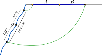
Figure 4: Schematic describes the appearance of the entanglement negativity island on the Planck brane for the case of two adjacent subsystems.

3.1.1 Adjacent subsystems

We start with two adjacent subsystems $A$ and $B$ of finite lengths $l_{1}$ and $l_{2}$ respectively in the radiation reservoirs and compute the holographic entanglement negativity between them using the eqs. 20 and 15. In particular, we investigate the qualitative nature of the entanglement negativity profiles for three distinct scenarios involving the subsystem sizes and the time. In this context we utilize the structures of the various RT surfaces supported by the subsystems in question described earlier in the diagrams fig. 3.

$\bm{(i)}$ Full system ($A\cup B$) fixed, common point varied

We first consider the case where the common point between the adjacent subsystems $A$ and $B$ is varied at a constant time slice while keeping the subsystem $A\cup B$ fixed which covers the entire reservoirs. In this scenario, we compute the holographic entanglement negativity between the subsystems $A$ and $B$ utilizing the eqs. 20 and 15. We observe that our results in this context reproduces the analogue of the Page curve for the entanglement negativity as depicted in fig. 5(a).

In this scenario, the entanglement negativity profile consists of five phases due to the various structures of the RT surfaces supported by the subsystems under consideration. The expressions for the corresponding entanglement negativity in these phases are listed in the appendix B. In what follows, we discuss these distinct phases of the entanglement negativity profile in details.

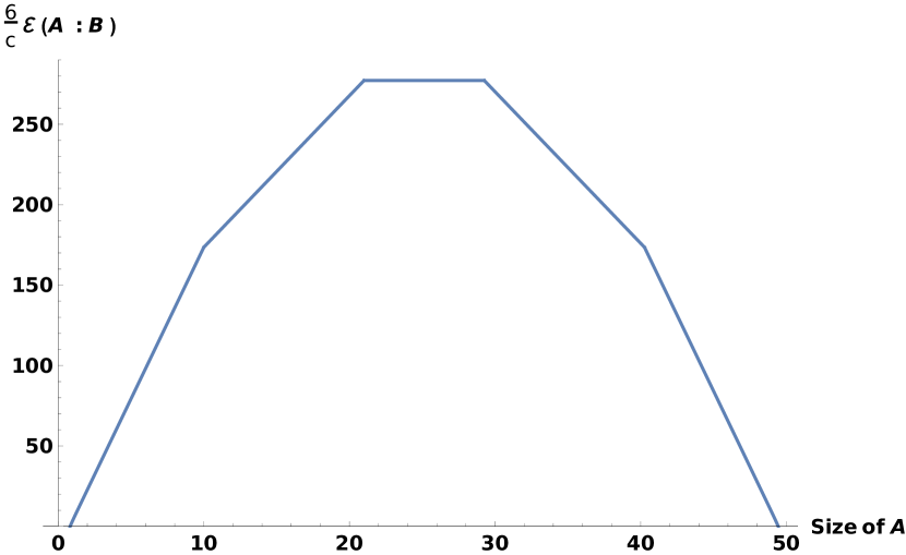
(a) Page curve for the entanglement negativity where we have considered $A\cup B=[.01L,.99L]$ at $t=15$.

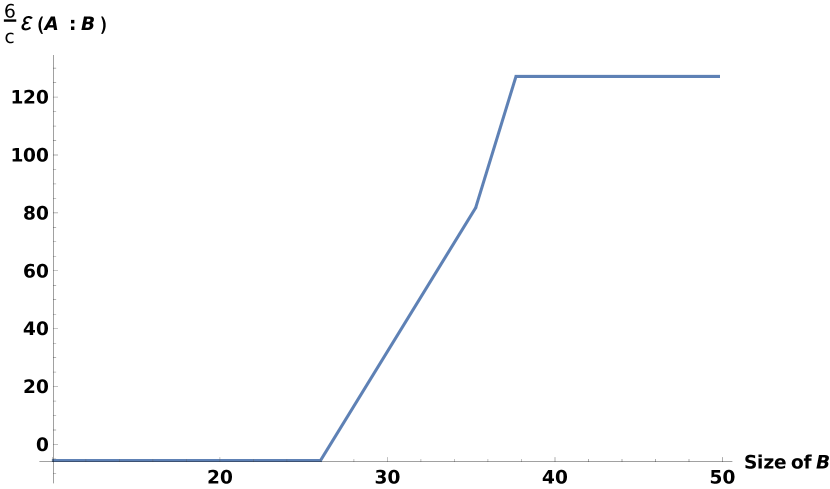
(b) Profile of the entanglement negativity with respect to the size of $B$ where we have considered $A=[.01L,.15L]$ at $t=20$.

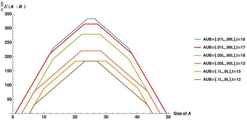
(c) Page curves for entanglement negativity for different sizes of $(A\cup B)^{c}$ and different times.

Figure 5: Here $\beta=1$, $c=500$, $\phi_{0}=\frac{30c}{6}$, $\phi_{r}=\frac{30}{\pi}$, $L=\frac{16\pi}{\beta}$, $\epsilon=.001$.

Phase 1: In the first phase, the dominating contribution to the entanglement entropy for the subsystem $A$ arises from dome-type RT surfaces, whereas the subsystems $B$ and $A\cup B$ support $ab$-type RT surfaces each as depicted in fig. 6. Interestingly, here the size of the subsystem $A$ is very small compared to the size of $B$ such that this phase does not admit any island region corresponding to the subsystem $A$. However, this phase involves entanglement entropy islands corresponding to the subsystem $B$ and $A\cup B$ which are located on both the Planck branes. In this case the entanglement negativity between the subsystems $A$ and $B$ is governed by the degrees of freedom of the subsystem $A$. Note that as we shift the common point, the number of Hawking modes captured by the subsystem $A$ and its $CFT_{2}$-degrees of freedom increase accordingly. Hence we observe a linearly rising behaviour in the corresponding entanglement negativity profile with the increasing size of the subsystem $A$ as exhibited in fig. 5(a).

Phase 2: Next we proceed to the second phase where the subsystems $A$ and $A\cup B$ still support dome and $ab$-type RT surfaces respectively, whereas the subsystem $B$ now admits $b$-bulk type RT surfaces as shown in fig. 6. Consequently, this phase includes an entanglement negativity island $I_{\varepsilon}(A)$ corresponding to the subsystem $A$ which is located on the $a$-brane. This negativity island contains the entire interior region of the $a$-black hole. Note that in this phase, the entanglement negativity between the subsystems $A$ and $B$ is governed by the degrees of freedom present in the region $A\cup I_{\varepsilon}(A)$. This is determined by the number of interior Hawking modes captured by the negativity island $I_{\varepsilon}(A)$ whose corresponding pairs are located in $(A\cup I_{\varepsilon}(A))^{c}$ and by the $CFT_{2}$-degrees of freedom present in $A\cup I_{\varepsilon}(A)$. In this case, as we increase the size of the subsystem $A$, the number of interior Hawking modes of $A\cup I_{\varepsilon}(A)$ decreases due to a purification by their corresponding pairs from the exterior region which are now transferred to the region $A\cup I_{\varepsilon}(A)$. However, the number of Hawking modes coming from the $b$-black hole simultaneously increases in the region $A\cup I_{\varepsilon}(A)$ with its increasing size which tends to cancel the preceding decreasing effect. Consequently, the degrees of freedom of the region $A\cup I_{\varepsilon}(A)$ are now determined only by the $CFT_{2}$-degrees of freedom which increases linearly with the shift of the common point between the adjacent subsystems. As a result, we observe a linearly rising behaviour in the corresponding entanglement negativity profile with a growth rate smaller than the previous phase.

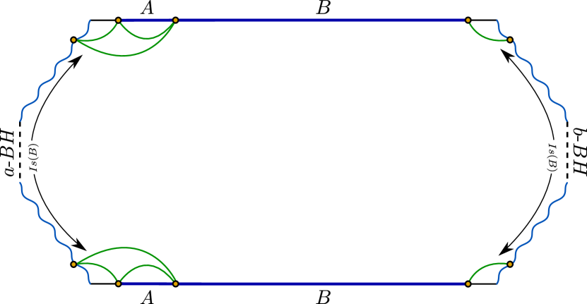
(a) Phase-1

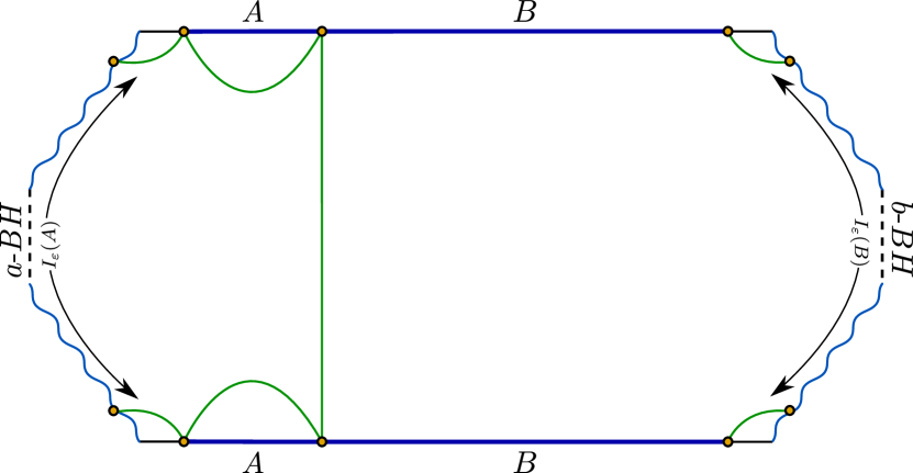
(b) Phase-2

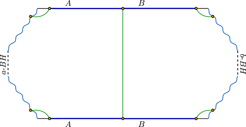
(c) Phase-3

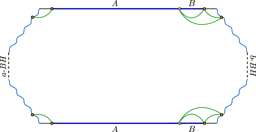
(d) Phase-4

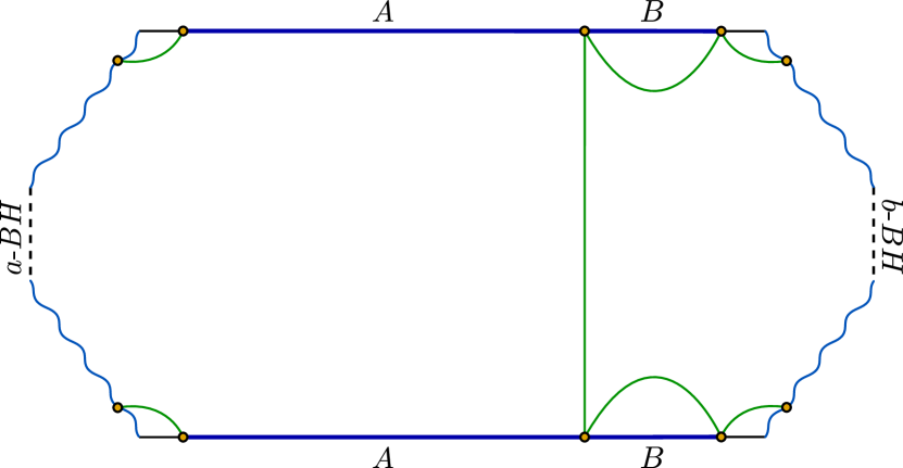
(e) Phase-5

Figure 6: Schematic depicts all the phases of the entanglement negativity for two adjacent subsystems where the common point between them is varied. The RT surfaces supported by the adjacent subsystems are denoted by the green geodesics. Note that these geodesics corresponding to the subsystems indicate the locations of the island regions on the Planck branes.

Phase 3: In the third phase (fig. 6), the RT surfaces supported by the subsystems $A$, $B$ and $A\cup B$ are $a$-$bulk$, $b$-$bulk$ and $ab$-type respectively. Here the size of the subsystem $A$ is comparable to the size of $B$ such that they are maximally entangled. This is a characteristic of tripartite entanglement where the tripartition is defined by the subsystems $A$, $B$ and $(A\cup B)^{c}$. Hence in this phase, the degrees of freedom present in the subsystems $A$ and $B$ are entangled with the degrees of freedom of the subsystem $(A\cup B)^{c}$ as the common point is shifted. Therefore this corresponds to a constant behaviour of the entanglement negativity profile as depicted in fig. 5(a).

Phase 4 and Phase 5: As depicted in fig. 6, the RT surfaces for the subsystems $A$ and $B$ in these two phases are interchanged with each other as compared to the first two phases. Hence, the corresponding entanglement negativity profile may be interpreted in a similar fashion as for the first two phases with the roles of the subsystems $A$ and $B$ exchanged.

We may further extend our analysis of the tripartite entanglement by considering different times and various sizes of the subsystem $(A\cup B)^{c}$. At a fixed time, we observe that the height of the plateau region of the corresponding entanglement negativity profile decreases with the increase in the size of the subsystem $(A\cup B)^{c}$ as exhibited in fig. 5(c). This behavior is consistent since the available degrees of freedom in the subsystems $A$ and $B$ entangled between themselves, decreases with the increasing size of $(A\cup B)^{c}$. On the other hand for a fixed size of the subsystem $(A\cup B)^{c}$ the height of the plateau region rises with increasing time. Once again this is consistent since the number of Hawking modes in all the subsystems rise with increasing time which corresponds to a larger entanglement between the subsystems.

In addition, with smaller size of the subsystem $(A\cup B)^{c}$, the height of the plateau region changes rapidly with a small change in time. However for larger size of $(A\cup B)^{c}$, we need to increase the time sufficiently such that it changes the height of the plateau region. This character of the entanglement negativity profile is again consistent since the subsystem $(A\cup B)^{c}$ can accommodate a fewer number of Hawking modes when its size is very small whereas a large number of Hawking modes can be accumulated in the subsystems $A$ and $B$ due to their larger sizes. Consequently as time increases, most of the newly created Hawking modes are collected by the subsystems $A$ and $B$ and thus increase the height of the Plateau region rapidly. However, for a larger size of the subsystem $(A\cup B)^{c}$, the accommodation for the Hawking modes is larger such that it may now capture more newly created Hawking modes with increasing time and as a result the height of the plateau region changes very slowly as time increases (fig. 5(c)).

$\bm{(ii)}$ Subsystem $\bm{A}$ fixed, $\bm{B}$ varied

In this scenario, we consider the length $l_{1}$ of the subsystem $A$ to be fixed at a constant time slice and investigate the behaviour of the holographic entanglement negativity while increasing the length $l_{2}$ of the subsystem $B$. The corresponding entanglement negativity profile is depicted in fig. 5(b) which consists of four distinct phases due to the various structures of the RT surfaces supported by the subsystems in question. The expressions for the holographic entanglement negativity between $A$ and $B$ in these phases, obtained through the eqs. 20 and 15, are listed in the appendix B. In what follows we now analyze these phases in detail.

Phase 1: We begin with the first phase where the RT surfaces for the subsystems $A$, $B$ and $A\cup B$ are $dome$-type each (fig. 7). Here the size of the subsystems $A$ and $B$ are very small and hence $A\cup B$ is far smaller than its complement $(A\cup B)^{c}$ which implies a vanishingly small entanglement negativity between the adjacent subsystems in question.

Phase 2: In the second phase, the subsystems $A$ and $B$ still support dome-type RT surfaces whereas the subsystem $A\cup B$ admits $a$-bulk type RT surfaces. Consequently, this phase includes entanglement negativity islands $I_{\varepsilon}(A)$ and $I_{\varepsilon}(B)$ on the $a$-brane corresponding to the subsystems $A$ and $B$ respectively. The exterior regions of the $a$-black hole constitutes the island $I_{\varepsilon}(A)$ on the $a$-brane, whereas $I_{\varepsilon}(B)$ involves the entire interior region of the $a$-black hole. In this context, the ratio of $l_{1}$ to $l_{2}$ decreases with increasing length $l_{2}$ of the subsystem $B$ and consequently the ratio of the size of $I_{\varepsilon}(A)$ to the size of $I_{\varepsilon}(B)$ decreases accordingly. Note that in this phase the entanglement negativity between the subsystems $A$ and $B$ is governed by the degrees of freedom of $B\cup I_{\varepsilon}(B)$. Now as we increase $l_{2}$, the number of interior Hawking modes captured by the negativity island $I_{\varepsilon}(B)$ decreases due to a purification by their exterior partners which are located in the region $(B\cup I_{\varepsilon}(B))^{c}$. This purification arises since the exterior partners are transferred to the region $B\cup I_{\varepsilon}(B)$ as the length $l_{2}$ of the subsystem $B$ increases. However, an equal number of Hawking modes from the $b$-black hole are transferred to the region $B\cup I_{\varepsilon}(B)$ simultaneously. Consequently, the degrees of freedom in the region $B\cup I_{\varepsilon}(B)$ are determined only by the $CFT_{2}$-degrees of freedom which increase with the increasing size of the subsystem $B$. Accordingly, the corresponding entanglement negativity profile rises linearly as depicted in fig. 5(b).

Phase 3: In this phase, the dominant contributions to the entanglement entropies of the subsystems $A$ and $B$ still arise from $dome$-type RT surfaces, whereas the subsystem $A\cup B$ now supports $ab$-type RT surfaces. Hence this phase admits an entanglement negativity island $I_{\varepsilon}(B)$ located on both the branes corresponding to the subsystem $B$ as shown in fig. 7. This negativity island $I_{\varepsilon}(B)$ contains the entire interior regions of both the black holes. Furthermore this phase also includes an entanglement negativity island $I_{\varepsilon}(A)$ corresponding to the subsystem $A$ (fig. 7), which involves only the exterior regions of the $a$-black hole. In this scenario, the entanglement negativity between the subsystems $A$ and $B$ is governed by the degrees of freedom of the region $A\cup I_{\varepsilon}(A)$. Interestingly, with increasing length $l_{2}$ of the subsystem $B$, the island region $I_{\varepsilon}(A)$ increases in size. Consequently, the number of Hawking modes and the $CFT_{2}$-degrees of freedom present in $A\cup I_{\varepsilon}(A)$ increase with the increasing length $l_{2}$ of the subsystem $B$. Hence we observe the corresponding entanglement negativity profile to rise linearly with a growth rate higher than the previous phase.

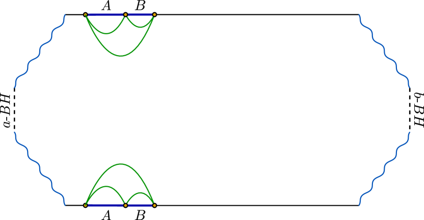
(a) Phase-1

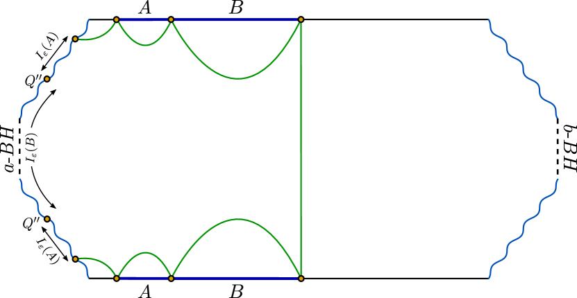
(b) Phase-2

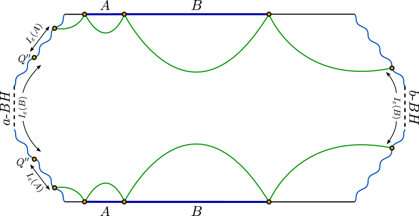
(c) Phase-3

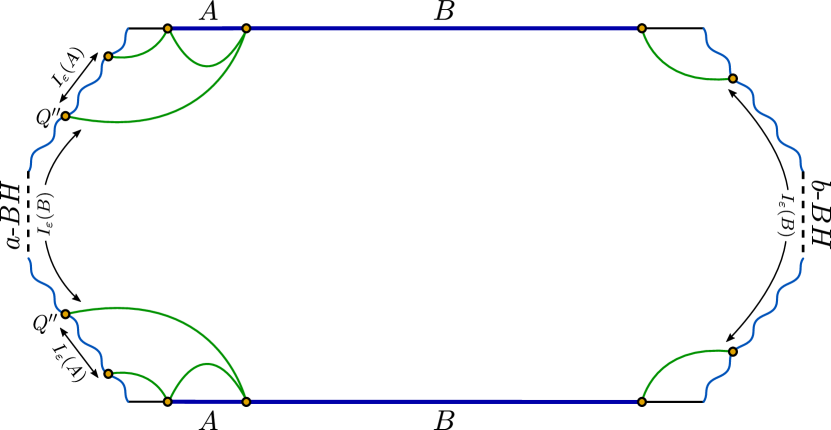
(d) Phase-4

Figure 7: The diagram shows the possible phases of the entanglement negativity profile for the case of two adjacent subsystems where the size of the subsystem $B$ is varied.

Phase 4: Finally in the last phase, the RT surfaces for the subsystems $B$ and $A\cup B$ are identified as $ab$-type each, however the subsystem $A$ still supports $dome$-type RT surfaces as depicted in fig. 7. Hence, this phase includes entanglement entropy islands for the subsystems $B$ and $A\cup B$, located on both of the Planck branes. Consequently, we have an entanglement negativity island $I_{\varepsilon}(A)$ corresponding to the subsystem $A$, which involves the exterior regions of the $a$-black hole. Once again the entanglement negativity in this phase is governed by the degrees of freedom of the region $A\cup I_{\varepsilon}(A)$. As we increase the length $l_{2}$, the size of the negativity island $I_{\varepsilon}(A)$ remains fixed which indicates that the number of the degrees of freedom in the region $A\cup I_{\varepsilon}(A)$is constant. Consequently, the corresponding entanglement negativity between the subsystems $A$ and $B$ exhibits a constant behaviour as shown in fig. 5(b).

$\bm{(iii)}$ Subsystems $\bm{A}$ and $\bm{B}$ fixed, time varied

We conclude our analysis with the case where the lengths $l_{1}$ and $l_{2}$ of the two adjacent subsystems $A$ and $B$ respectively are fixed and the time $t$ is varied. In this context, we consider two sub cases with equal and unequal lengths of the subsystems $A$ and $B$ and obtain the corresponding holographic entanglement negativity between them utilizing the eqs. 20 and 15. Since the subsystem sizes are fixed in this scenario, the $CFT_{2}$-degrees of freedom for the subsystems are also fixed and hence irrelevant for the description of the various phases of the entanglement negativity profiles. The only effect on the profiles arise from the Hawking modes arriving from both the black holes to the subsystems and this is utilized to analyze the corresponding entanglement negativity profiles depicted in fig. 8.

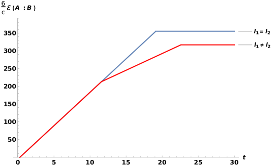
Figure 8: Page curves for entanglement negativity with respect to time $t$. Here $\beta=1$, $c=500$, $\phi_{0}=\frac{30c}{6}$, $\phi_{r}=\frac{30}{\pi}$, $L=\frac{16\pi}{\beta}$, $\epsilon=.001$, $A=[.01L,.5L]$ and $B=[.5L,.99L]$ (for $l_{1}=l_{2}$), $A=[.01L,.35L]$ and $B=[.35L,.99L]$ (for $l_{1}\neq l_{2}$).

(a) For $\bm{l_{1}=l_{2}}$

For the case of two equal lengths subsystems $A$ and $B$, we observe that the Page curve for the entanglement negativity consists of two phases as depicted in fig. 8. The expressions for the holographic entanglement negativity in the corresponding phases are listed in the appendix B. In what follows, we comprehensively analyze these phases.

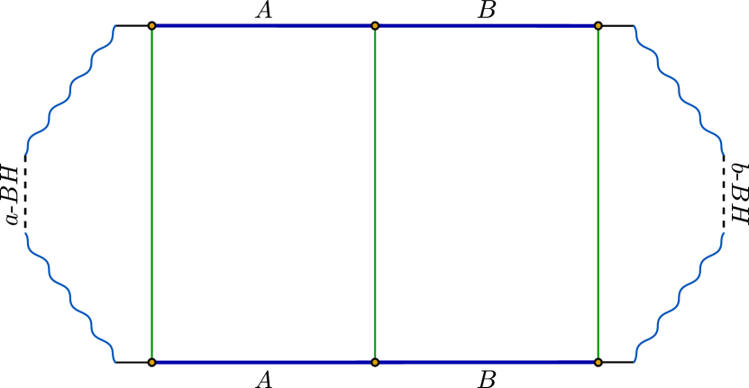
(a) Phase-1(a)

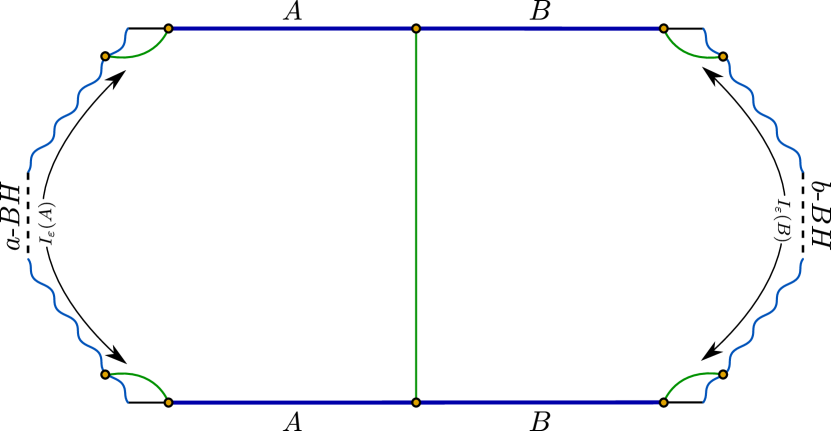
(b) Phase-1(b)

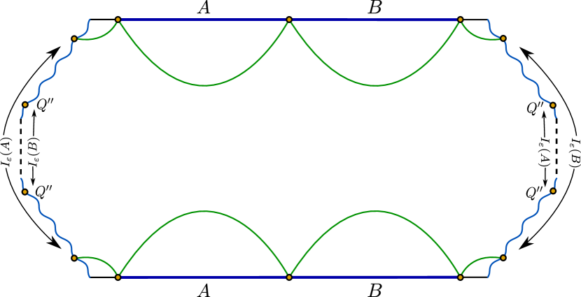
(c) Phase-2

Figure 9: Schematic depicts all the possible phases of the entanglement negativity between two adjacent subsystems with equal sizes as time increases.

Phase 1: This phase contains two intermediate sub phases due to the various structures of the RT surfaces supported by the subsystems in question. At early times, the subsystems $A$, $B$ and $A\cup B$ support bulk-type RT surfaces each (fig. 9). This sub phase does not include any island regions corresponding to the subsystems mentioned above. The number of Hawking modes from both the black holes accumulating in the two subsystems increases linearly with increasing time. Hence, the corresponding entanglement negativity profile rises linearly as time increases. We proceed to the second sub phase where the dominant contributions to the entanglement entropies of the subsystems $A$, $B$ and $A\cup B$ arise from $a$-$bulk$, $b$-$bulk$ and $ab$-type RT surfaces respectively. Hence this sub phase includes entanglement negativity islands $I_{\varepsilon}(A)$ and $I_{\varepsilon}(B)$ corresponding to the subsystems $A$ and $B$ respectively as shown in fig. 9. Here the island $I_{\varepsilon}(A)$ contains the entire interior region of the $a$-black hole whereas the other island $I_{\varepsilon}(B)$ includes the entire interior region of the $b$-black hole. In this case, the entanglement negativity between the subsystems is governed by the degrees of freedom in the region $A\cup I_{\varepsilon}(A)$ or $B\cup I_{\varepsilon}(B)$. Note that the degrees of freedom in the region $A\cup I_{\varepsilon}(A)$ are determined by the interior Hawking modes captured by the negativity island $I_{\varepsilon}(A)$ whose exterior partners are located in $(A\cup I_{\varepsilon}(A))^{c}$ and by the Hawking modes arriving from the $b$-black hole. These degrees of freedom increase with time which confirms the linear rise of the corresponding Page curve as depicted in fig. 8. The description for the second sub phase from the perspective of the degrees of freedom of the region $B\cup I_{\varepsilon}(B)$ is analogous to the arguments mentioned above which again justifies the linear rising behaviour of the corresponding Page curve.

Phase 2: In the second phase, the subsystems $A$ and $B$ support $dome$-type RT surfaces each whereas the subsystem $A\cup B$ still admits $ab$-type RT surfaces (fig. 9). This phase includes an entanglement entropy island for the subsystem $A\cup B$ and hence we have entanglement negativity islands $I_{\varepsilon}(A)$ and $I_{\varepsilon}(B)$ corresponding to the subsystems $A$ and $B$ respectively. Here each of the negativity islands $I_{\varepsilon}(A)$ and $I_{\varepsilon}(B)$ contains the entire interior regions of both the black holes. Hence this phase corresponds to an overlap between the negativity island regions $I_{\varepsilon}(A)$ and $I_{\varepsilon}(B)$ as shown in fig. 9. This is an extremely interesting and novel scenario which has not been reported in earlier literatures on the island constructions. Once again in this phase, the entanglement negativity between the subsystems is governed by the degrees of freedom of the region $A\cup I_{\varepsilon}(A)$ or $B\cup I_{\varepsilon}(B)$. Note that the degrees of freedom of the region $A\cup I_{\varepsilon}(A)$ are determined by the interior Hawking modes captured by the negativity island $I_{\varepsilon}(A)$ whose exterior partners are located in $(A\cup I_{\varepsilon}(A))^{c}$. At late times, the number of ingoing and outgoing Hawking modes in the region $A\cup I_{\varepsilon}(A)$ become equal such that its degrees of freedom remains constant throughout this phase. Consequently, the Page curve for the entanglement negativity exhibits a constant behaviour as depicted in fig. 8. Once again, the description for this phase from the perspective of the degrees of freedom of the region $B\cup I_{\varepsilon}(B)$ is analogous to the arguments mentioned above which again justifies the constant behaviour of the corresponding Page curve. Note that in this phase, other candidates for the entanglement negativity islands corresponding to the subsystems $A$ and $B$ may be considered analogous to those observed in the phase-1(b). However, with those negativity islands, the corresponding entanglement negativity profile continues to rise linearly and thus do not provide a consistent interpretation for the phase-2.

(b) For $\bm{l_{1}\neq l_{2}}$

Next we consider two unequal lengths of the subsystems $A$ and $B$ and observe that the corresponding Page curve for the entanglement negativity consists of three consecutive phases. Again we refer to the appendix B for the entanglement negativity expressions obtained in these distinct phases. In the following, we now explore these phases in detail.

Phase 1: In this phase (fig. 10), the various structures of the RT surfaces supported by the subsystems and the corresponding interpretation in terms of the Hawking radiation are identical to the first phase of the previous sub case.

Phase 2: We proceed to the second phase where the dominant contributions to the entanglement entropy of the subsystems $A$, $B$ and $A\cup B$ arise from dome, $b$-bulk and $ab$-type RT surfaces respectively. Hence, this phase includes an entanglement negativity island $I_{\varepsilon}(B)$ corresponding to the subsystem $B$ as depicted in fig. 10. Here the negativity island $I_{\varepsilon}(B)$ contains the entire interior region of both the black holes. Note that the entanglement negativity between the subsystems $A$ and $B$ in this phase is governed by the degrees of freedom of the region $B\cup I_{\varepsilon}(B)$. These degrees of freedom are determined by the interior Hawking modes captured by the island $I_{\varepsilon}(B)$ whose exterior partners are located in $(B\cup I_{\varepsilon}(B))^{c}$. Now the number of outgoing Hawking modes is larger than the number of ingoing Hawking modes in the region $B\cup I_{\varepsilon}(B)$. Hence the degrees of freedom of the region $B\cup I_{\varepsilon}(B)$ increase with time at a smaller rate than the previous phase which corresponds to the increasing behaviour of the Page curve as depicted in fig. 8.

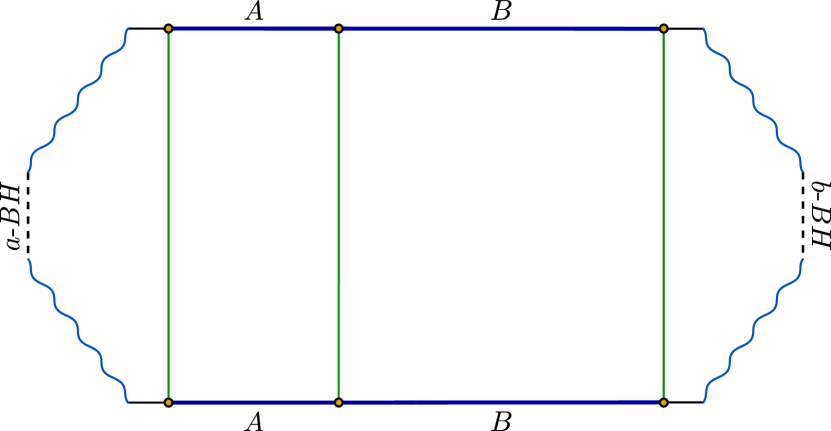
(a) Phase-1(a)

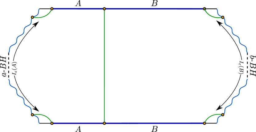
(b) Phase-1(b)

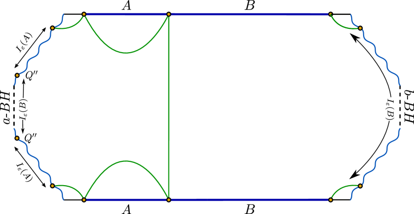
(c) Phase-2

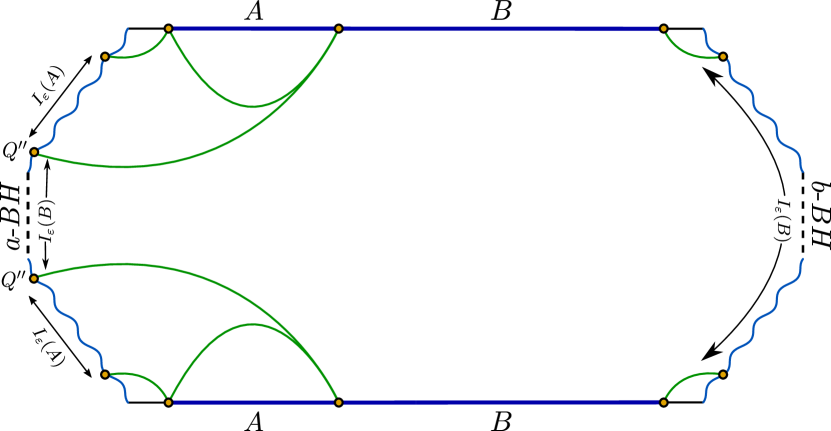
(d) Phase-3

Figure 10: Different phases of the entanglement negativity between two adjacent subsystems with unequal sizes as time increases.

Phase 3: Finally in the last phase, the RT surfaces supported by the subsystem $B$ are $ab$-type whereas the subsystems $A$ and $A\cup B$ still admit dome and $ab$-type RT surfaces respectively (fig. 10). Once again this phase includes an entanglement negativity island $I_{\varepsilon}(B)$ for the subsystem $B$ with a description similar to the previous phase. In this scenario, the entanglement negativity between the subsystems is again governed by the degrees of freedom of the region $B\cup I_{\varepsilon}(B)$ which are determined similarly as in the previous phase. At late times, the number of ingoing and outgoing Hawking modes in the region $B\cup I_{\varepsilon}(B)$ are equal such that its degrees of freedom remain constant throughout this phase. Consequently, the Page curve for the entanglement negativity exhibits a constant behaviour as depicted in fig. 8.

3.1.2 Disjoint subsystems

Next we consider a mixed state configuration of two disjoint subsystems $A$ and $B$ with finite lengths $l_{1}$ and $l_{2}$ respectively where a subsystem $C$ with length $l_{c}$ is sandwiched between them. In this context, we utilize the eqs. 25 and 15 to obtain the holographic entanglement negativity between the subsystems $A$ and $B$ for three distinct scenarios involving the subsystem sizes and the time. Furthermore, we describe the qualitative nature of the corresponding entanglement negativity profiles in these scenarios.

$\bm{(i)}$ Subsystem $\bm{A}$ fixed, $\bm{C}$ varied

We begin with the case where the length $l_{1}$ of the subsystem $A$ is fixed at a constant time slice and compute the holographic entanglement negativity between the subsystems $A$ and $B$ with an increasing length ${l_{c}}$ of the subsystem $C$. We observe four consecutive phases of the entanglement negativity profile as depicted in fig. 11(a) due to the various structures of the RT surfaces supported by the subsystems in question. Utilizing the eqs. 25 and 15, we obtain the expressions for the corresponding entanglement negativity in these phases which are listed in the appendix B. In what follows, we describe these phases of the entanglement negativity profile in detail.

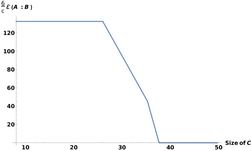
(a) Entanglement negativity with respect to the size of $C$ where we have considered $B\cup C=[.15L,.99L]$ and $A\cup B\cup C=[.01L,.99L]$.

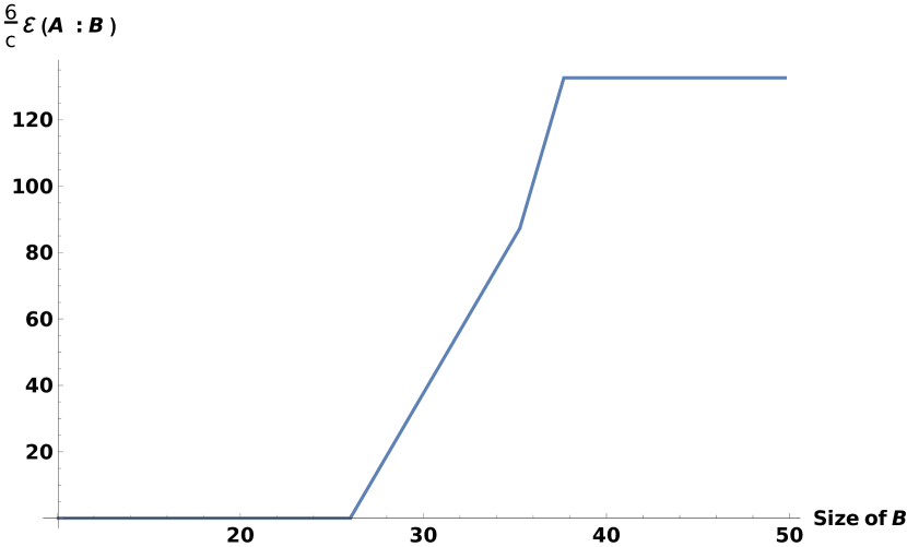
(b) Entanglement negativity with respect to the size of $B$ where we have considered $C=[.15L,.2L]$.

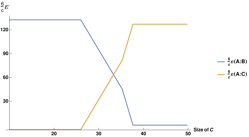
(c) Entanglement negativity between different subsystems where we have considered $A=[.01L,.15L]$, $B\cup C=[.15L,.99L]$ and $A\cup B\cup C=[.01L,.99L]$.

Figure 11: Here $\beta=1$, $c=500$, $t=20$, $\phi_{0}=\frac{30c}{6}$, $\phi_{r}=\frac{30}{\pi}$, $L=\frac{16\pi}{\beta}$, $\epsilon=.001$, $A=[.01L,.15L]$.

Phase 1: In the first phase, the RT surfaces for the subsystems $A\cup C$ and $C$ are dome-type each whereas the subsystems $B\cup C$ and $A\cup B\cup C$ support $ab$-type RT surfaces. Here the size of the subsystem $A\cup C$ is very small compared to the size of $B$ such that this phase does not correspond to any island region for the subsystem $A\cup C$. In this phase, the entanglement negativity between the subsystems $A$ and $B$ is governed by the degrees of freedom of the subsystem $A$. Note that the corresponding degrees of freedom of the subsystem $A$ remain constant since the number of Hawking modes arriving from both the black holes together with the $CFT$ degrees of freedom do not change with the increasing length $l_{c}$. Consequently the entanglement negativity profile in this phase remains constant as depicted in fig. 11(a).

Phase 2: Next we proceed to second phase where the subsystems $A\cup C$ and $C$ admit $a$-bulk and dome-type RT surfaces respectively whereas the subsystems $B\cup C$ and $A\cup B\cup C$ still support $ab$-type RT surfaces. Consequently, this phase involves an entanglement negativity island $I_{\varepsilon}(B)$ on the $b$-brane corresponding to the subsystem $B$. This island $I_{\varepsilon}(B)$ involves the entire interior region of the $b$-black hole. The entanglement negativity between the subsystems $A$ and $B$ in this phase is governed by the degrees of freedom of the region $B\cup I_{\varepsilon}(B)$. As we increase $l_{c}$, the number of Hawking modes arriving from the $a$-black hole leave the region $B\cup I_{\varepsilon}(B)$. However an equal number of interior Hawking modes captured by the negativity island $I_{\varepsilon}(B)$ whose partners are located in $(B\cup I_{\varepsilon}(B))^{c}$ increase simultaneously. Consequently, the degrees of freedom of the region $B\cup I_{\varepsilon}(B)$ is determined only by the $CFT_{2}$-degrees of freedom which decrease with the increasing length $l_{c}$ as the size of the subsystem $B$ decreases. Accordingly, the corresponding entanglement negativity profile decreases linearly as depicted in fig. 11(a).

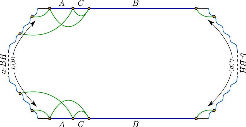
(a) Phase-1

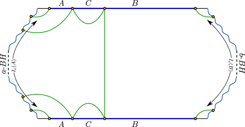
(b) Phase-2

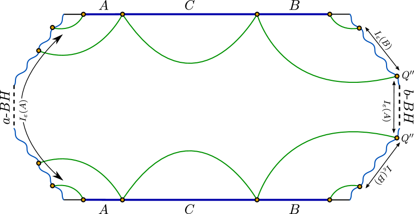
(c) Phase-3

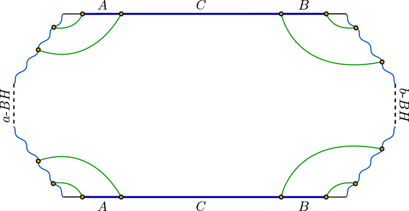
(d) Phase-4

Figure 12: The possible phases of the entanglement negativity between two disjoint subsystems $A$ and $B$ while increasing the size of the subsystem $C$ sandwiched between them.

Phase 3: In this phase the dominant contributions to the entanglement entropies of the subsystems $A\cup C$, $B\cup C$ and $A\cup B\cup C$ arise from $ab$-type RT surfaces each whereas the subsystem $C$ still supports dome-type RT surfaces. This phase includes an entanglement negativity island $I_{\varepsilon}(B)$ for the subsystem $B$ located on the exterior region of the $b$-black hole. Once again the entanglement negativity between the subsystems in this phase is governed by the degrees of freedom of the region $B\cup I_{\varepsilon}(B)$. Hence the number of Hawking modes arriving from both the black holes and the $CFT_{2}$-degrees of freedom present in the region $B\cup I_{\varepsilon}(B)$ decrease with increasing length $l_{c}$ of the subsystem $C$ as the size of the subsystem $B$ decreases. Consequently, we observe a linear decreasing profile of the corresponding entanglement negativity with a rate higher than the previous phase as depicted in fig. 11(a).

Phase 4: In the last phase, the RT surfaces for the subsystems $A\cup C$, $B\cup C$, $A\cup B\cup C$ and $C$ are identified as $ab$-type each. Consequently, the corresponding entanglement wedges of the subsystems $A$ and $B$ are disconnected from each other in this phase which indicates a zero entanglement negativity between them. On a separate note, here the subsystems $A$ and $B$ are very small and located far away from each other such that they do not develop any entanglement between themselves.

We now discuss an interesting issue by comparing the above results with those discussed in subsection 3.1 where the entanglement negativity between two adjacent subsystems $A$ and $C$ was analyzed. This comparison is depicted in figure-11(c).

We find that the entanglement negativity between the subsystems $A$ and $C$ follows identical behaviour as discussed in subsection 3.1. Note that the negativity between the subsystems $A$ and $B\cup C$ is constant throughout our analysis since we have fixed their sizes $l_{1}$, $l_{c}+l_{2}$ respectively and the time $t$. Now, with the increasing length $l_{c}$, the size of the subsystem $B$ decreases accordingly. Hence the degrees of freedom of $B$ are eventually transferred to the subsystem $C$ as $l_{c}$ increases. As a result the entanglement negativity between the subsystems $A$ and $B$ decreases while the entanglement negativity between the subsystems $A$ and $C$ is increasing as depicted in fig. 11(c).

$\bm{(ii)}$ Subsystems $\bm{A}$ and $\bm{C}$ fixed, $\bm{B}$ varied

In this scenario, the lengths $l_{1}$ and $l_{c}$ of the subsystems $A$ and $C$ are fixed at a constant time slice. We then compute the holographic entanglement negativity between the two disjoint subsystems $A$ and $B$ with an increase in the length $l_{2}$ of the subsystem $B$ utilizing the eqs. 25 and 15. In this case, we observe four consecutive phases of the entanglement negativity profile as exhibited in fig. 11(b). Once again the expressions for the corresponding entanglement negativity in these distinct phases are listed in the appendix B. It is interesting to note that in this scenario, the profile of the entanglement negativity follows the behaviour similar to the adjacent case discussed in the subsection 3.1 where we fixed the size of the subsystem $A$ and varied the size of $B$. Consequently in the present case, the corresponding phases may be explained analogously in terms of the Hawking radiations.

$\bm{(iii)}$ Subsystems $\bm{A}$, $\bm{B}$ and $\bm{C}$ fixed, time varied

We conclude our analysis with the following case where the sizes of all the subsystems are fixed. For this scenario we compute the holographic entanglement negativity between the disjoint subsystems $A$ and $B$ with increasing time utilizing the eqs. 25 and 15. In particular, we obtain two Page curves for the corresponding entanglement negativity for two sub cases with equal and unequal lengths of the subsystems $A$ and $B$ as depicted in fig. 15. In these scenarios, the $CFT_{2}$-degrees of freedom are irrelevant for the description of the entanglement negativity profiles since all the subsystem sizes are fixed. Hence the only effect on these profiles arise from the Hawking modes arriving from both the black holes.

(a) For $\bm{l_{1}=l_{2}}$

For the case of two equal lengths subsystems, the Page curve for the entanglement negativity between the subsystems $A$ and $B$ consists of three consecutive phases and the expressions for the same in these phases are listed in the appendix B. In the following, we analyze these phases in detail.

Phase 1: In the first phase (fig. 13), the dominant contributions to the entanglement entropies of all the subsystems arise from bulk-type RT surfaces each. Hence the entanglement wedges of the subsystems $A$ and $B$ are disconnected in this phase. Consequently the entanglement negativity between the subsystems in this case is zero as depicted in fig. 15. On a separate note, at initial times the number of Hawking modes present in the subsystems $A$ and $B$ are very small such that they do not lead to a significant entanglement between the subsystems.

Phase 2: This phase consists of two sub phases due to the various structures of the RT surfaces supported by the subsystems as depicted in fig. 13. In the first sub phase, the RT surfaces for the subsystems $A\cup C$, $B\cup C$ and $A\cup B\cup C$ are still identified as bulk-type whereas the subsystem $C$ now supports dome-type RT surfaces. In the second sub phase the dominant contributions to the entanglement entropies of the subsystems $A\cup C$, $B\cup C$, $A\cup B\cup C$ and $C$ arise from $a$-bulk, $b$-bulk, $ab$ and dome-type RT surfaces respectively. The increasing behaviour of the corresponding entanglement negativity profile in these two sub phases follows the interpretations which are analogous to the first phase of the adjacent case described in subsection 3.1.

Phase 3: In the last phase, the Page curve for the entanglement negativity between the two disjoint subsystems $A$ and $B$ depicts a constant behaviour as exhibited in fig. 15. Here the RT surfaces supported by the subsystems $A\cup C$, $B\cup C$ and $C$ are dome type each whereas the subsystem $A\cup B\cup C$ admits $ab$ type RT surfaces (fig. 13). Once again, we refer to the second phase of the adjacent case described in subsection 3.1 to explain the constant behaviour of the corresponding entanglement negativity profile.

(a) Phase-1

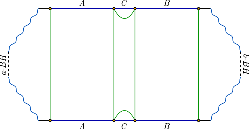
(b) Phase-2a

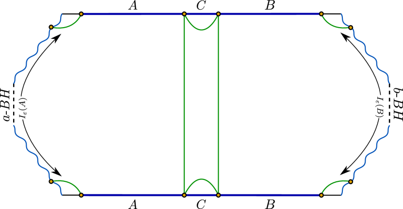
(c) Phase-2b

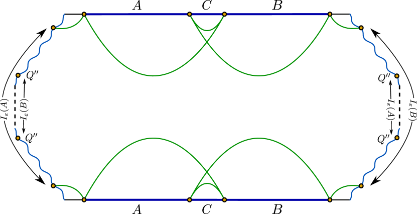
(d) Phase-3

Figure 13: The diagram shows the possible phases of the entanglement negativity between two disjoint subsystems with equal sizes as time increases.

(b) For $\bm{l_{1}\neq l_{2}}$

For the case of two unequal lengths subsystems $A$ and $B$, we observe that the Page curve for the entanglement negativity between them consists of four different phases as depicted in fig. 15. Once again the corresponding entanglement negativity expressions are listed in the appendix B. In what follows, we describe these phases in detail.

Phase 1 and Phase 2: In these phases (fig. 14), the RT surfaces supported by the subsystems and the description for the corresponding entanglement negativity profile are identical to the first two phases of the previous sub case.

Phase 3: In the third phase, the dominant contributions to the entanglement entropies of the subsystems $A\cup C$ and $C$ arise from dome-type RT surfaces each whereas the subsystems $B\cup C$ and $A\cup B\cup C$ admit $b$-bulk and $ab$ type RT surfaces respectively as shown in fig. 14. This phase includes entanglement negativity island $I_{\varepsilon}(A)$ corresponding to the subsystem $A$ located in the exterior regions of the $a$-black hole. However, the entanglement negativity island $I_{\varepsilon}(B)$ corresponding to the subsystem $B$ involve the entire interior regions of both the black holes. The explanation for the increasing behaviour of the corresponding entanglement negativity profile in this phase is similar to the second phase of the adjacent case discussed in subsection 3.1.

Phase 4: Finally in the last phase (fig. 14), the entanglement negativity between the subsystems $A$ and $B$ exhibits a constant behaviour which again may be explained similarly to that of the third phase of the adjacent case as discussed in subsection 3.1.

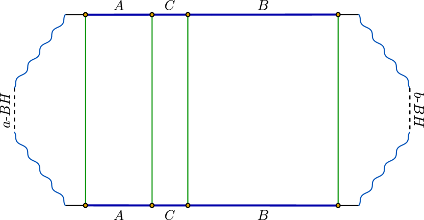
(a) Phase-1

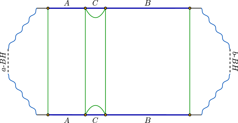
(b) Phase-2a

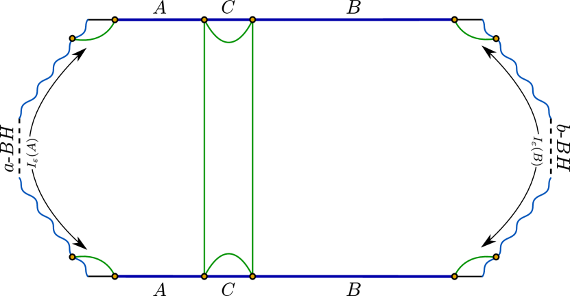
(c) Phase-2b

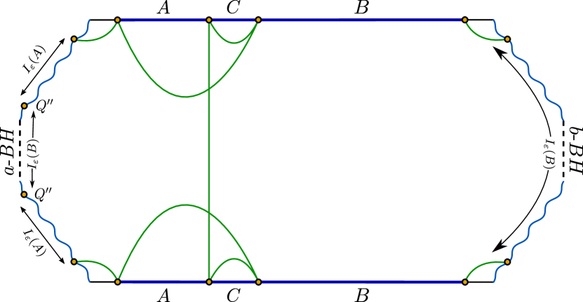
(d) Phase-3

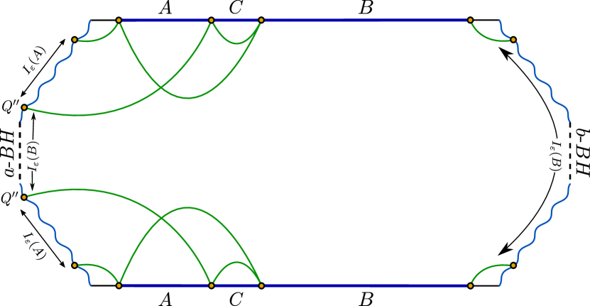
(e) Phase-4

Figure 14: The possible phases of the entanglement negativity between two disjoint subsystems with unequal sizes as time increases.

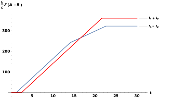
Figure 15: Page curves for entanglement negativity with respect to time $t$. Here $\beta=1$, $c=500$, $\phi_{0}=\frac{30c}{6}$, $\phi_{r}=\frac{30}{\pi}$, $L=\frac{16\pi}{\beta}$, $\epsilon=.001$, $A=[.01L,.45L]$ and $B=[.55L,.99L]$ (for $l_{1}=l_{2}$), $A=[.01L,.35L]$ and $B=[.4L,.99L]$ (for $l_{1}\neq l_{2}$).

4 Summary and Discussion

To summarize, we have investigated the holographic entanglement negativity for various finite temperature bipartite mixed states in a braneworld model of two communicating black holes. This construction involves two finite sized non-gravitating reservoirs coupled to two quantum dots at their boundaries at a finite temperature. These quantum dots constituted two copies of thermofield double states which interacted through the common reservoirs. The holographic dual of these quantum dots were described by JT gravity on two Plank branes with $AdS_{2}$ geometries. Interestingly, each non-gravitating reservoir together with a Planck brane appeared to be gravitating from the perspective of the other brane. These Planck branes involved two eternal JT black holes which were in communication through the shared reservoirs. In this configuration, the black hole and the reservoir regions supported identical matter $CFT_{2}$s with transparent boundary conditions. In this context, we obtained the holographic entanglement negativity for various bipartite mixed states of two adjacent and disjoint subsystems in the reservoirs for the above configuration. In this connection, we have analyzed the profiles of the generalized entanglement negativity for different scenarios involving the subsystem sizes and the time. The behaviour of the corresponding entanglement negativity profiles observed for the above scenarios were similar to that described in KumarBasak:2021rrx where the authors considered evaporating black holes in JT gravity through a geometrized island construction.

In appendix A, another model was described by a brane world geometry involving a bulk eternal $AdS_{3}$ BTZ black hole truncated by two Karch-Randall (KR) branes with two dimensional black holes induced from the higher dimension. These induced black holes were in communication through shared baths described by thermal $BCFT_{2}$s on a strip with different boundary conditions at either end constituting a thermofield double state Geng:2021iyq . We have computed the entanglement entropy for a subsystem with both of its end points located in the bulk of the $BCFT_{2}$s for the above configuration. Furthermore we also computed the holographic entanglement negativity for two adjacent and disjoint subsystems in the bath $BCFT_{2}$s using the holographic proposals described in Jain:2017aqk for different scenarios involving the subsystem sizes and the time. For these cases, we observed the behaviour of the entanglement negativity profiles similar to those described in KumarBasak:2021rrx .

We would like to emphasize that the presence of two black holes in these braneworld models lead to the appearance of extra phases in the Page curves for both the entanglement entropy and the entanglement negativity compared to configurations which support a single black hole. Note that the braneworld models considered by us are structurally distinct although both supported black holes communicating through shared radiation reservoirs. We considered a braneworld model Balasubramanian:2021xcm incorporating JT black holes on the Planck branes which were dual to quantum dots on either ends of finite sized $CFT_{2}$ radiation reservoirs. In this context it was possible to express an explicit island formula for the entanglement measures. However, in appendix A, we considered another braneworld model Geng:2021iyq involving two dimensional black holes on the KR branes induced from a higher dimensional BTZ black hole where an explicit island prescription for the entanglement measures can not be utilized although the final results for the Page curves are consistent with the expected island scenario. Note that the overall behaviour of the entanglement profiles were similar in these braneworld geometries. However, there were some interesting distinctions such as for the variation of the subsystem size in one of the cases, the corresponding Page curve for the entanglement negativity involved a plateau region for the braneworld model Balasubramanian:2021xcm due to the position independence of the entanglement entropy in contrast to the other model Geng:2021iyq . Additionally an interesting feature of tripartite entanglement was also observed for subsystems with comparable sizes for the case of Planck braneworld geometries Balasubramanian:2021xcm .

There are several interesting future directions to explore in connection with our results. A significant open issue involves the generalization of these braneworld construction to higher dimensions. Such an analysis although non trivial may reveal deeper insights into the structure of the mixed state entanglement in such communicating black hole/bath systems. Our analysis should also extend to models with defect $CFT$s on the EOW branes. Furthermore certain overlapping configurations observed for the entanglement negativity islands in some phases indicate some subtle characteristics of the structure of mixed state entanglement which needs more careful investigation using various toy models of black hole evaporation. We hope to return to these exciting issues in the near future.

5 Acknowledgement

We are grateful to Vinay Malvimat and Vinayak Raj for useful discussions. The work of GS is partially supported by the Dr. Jagmohan Garg Chair Professor position at the Indian Institute of Technology, Kanpur.

Appendix A Entanglement measures in braneworld model-II

In this section we first compute the entanglement entropy for a generic subsystem in the $BCFT_{2}$s Geng:2021iyq . Note that here we consider both the end points of the subsystem to be situated deep into the annular region of the $BCFT_{2}$s. Subsequently, we analyze the holographic entanglement negativity for various bipartite mixed states in the $BCFT_{2}$s at a finite temperature. The dual bulk space time for this construction is very complicated but in the high temperature limit this reduces to an eternal $AdS_{3}$ BTZ black hole Maldacena:2001kr ; Banados:1992wn as demonstrated in Geng:2021iyq . The bulk configuration involves two dimensional black holes on both the KR branes induced from the higher dimensional BTZ black hole Geng:2021iyq but with different temperatures due to the distinct boundary conditions at the two boundaries of the two dual $BCFT_{2}$s. Interestingly, these entanglement measures characterize the communication between the two induced black holes on the KR branes Geng:2021iyq .

A.1 Entanglement entropy and Page curve

We begin with the computations of the different contributions to the entanglement entropy for a generic subsystem at a finite temperature as mentioned above. In this connection, we first describe the field theory analysis for the entanglement entropy in the dual $BCFT_{2}$s following the method discussed in Geng:2021iyq . Furthermore we substantiate these field theory results from holographic computations of the entanglement entropy in the dual bulk geometry utilizing wedge holography.

A.1.1 Field theory computations

In this subsection, we consider a subsystem $A=A_{L}\cup A_{R}$ in the $BCFT_{L}$ and $BCFT_{R}$ with its end points located in the bulk of the annular region as shown in figure 16. These two $BCFT_{2}$s at a finite temperature constitute a thermofield double state as discussed in Geng:2021iyq . The twist operators $\bar{\Phi}_{n}\left(w_{L_{1}},\bar{w}_{L_{1}}\right)$, $\Phi_{n}\left(w_{L_{2}},\bar{w}_{L_{2}}\right)$, $\Phi_{n}\left(w_{R_{1}},\bar{w}_{R_{1}}\right)$, and $\bar{\Phi}_{n}\left(w_{R_{2}},\bar{w}_{R_{2}}\right)$ in this context are situated at the end points of the subsystem $A$. Note that, the motivation behind the choice of a generic subsystem mentioned above is to explore all the possible channels for a four point twist field correlator in the entanglement entropy expression discussed in eq. 29 in contrast to the article Geng:2021iyq . In the subsequent appendix, this would significantly lead to a rich phase structure for the holographic entanglement negativity of bipartite mixed states described by two adjacent and disjoint subsystems with all the end points located into the bulk of the bath $BCFT_{2}$s.

The above configuration of a generic subsystem in the bath $BCFT_{2}$s is considered in the complex $w$-plane where the boundary conditions on the two boundaries are denoted as $a$ and $b$ with a separation $L$ between the inner ($r_{I}$) and the outer radii ($r_{O}$) as depicted in fig. 16. At this moment, it would be beneficial to have a conformal map from annulus to a strip such that the techniques described in Geng:2021iyq can be utilized to obtain the entanglement entropy. However, there can never be any such transformation since the annulus generally has non zero modular parameter which should be preserved under such conformal mapping Geng:2021iyq ; Polchinski . Interestingly, if we consider the high temperature limit, the above mentioned mapping can still be accomplished. This corresponds to the limit of fixed $L=r_{O}-r_{I}$ and considering the inner radius of the annulus close to zero ($r_{I}/L\rightarrow 0$). The high temperature limit can also be achieved by considering the limit $r_{O}\rightarrow\infty$ and consequently $r_{I}/L\rightarrow 0$. The entanglement entropy of the subsystem $A=A_{L}\cup A_{R}$ can now be computed using a mapping of the $w$-plane to the UHP following the transformation

$$w=r_{I}\left(\frac{1}{z-\frac{i}{2}}-i\right)\,,$$ (28)

with $r_{I}$ being the inner radius of the annulus. Note that the corresponding transformation maps the inner and the outer radii to the real axis and to a point $z=\frac{i}{2}$ respectively on the UHP. This reduces the computation of the four point twist correlator on the annulus to that on the UHP. Note that here we restrict to a subset of the available channels with the assumption that the pair of intervals in the TFD copy always mapped onto each other by a rotation of the annulus . Consequently, utilizing the transformation in eq. 28, we obtain the contributions to the entanglement entropy from the four point function as follows

$$S_{A}=\lim_{n\rightarrow 1}\frac{1}{1-n}\log(\left<\Phi_{n}\left(z_{R_{1}},\bar{z}_{R_{1}}\right)\bar{\Phi}_{n}\left(z_{R_{2}},\bar{z}_{R_{2}}\right)\Phi_{n}\left(z_{L_{2}},\bar{z}_{L_{2}}\right)\bar{\Phi}_{n}\left(z_{L_{1}},\bar{z}_{L_{1}}\right)\right>^{b}_{\text{UHP},a})\,,$$ (29)

where the lower and the upper indices $a,b$ represent the boundary conditions corresponding to the two boundaries of the $BCFT_{2}$s. It is possible to identify seven distinct contributions to the corresponding entanglement entropy from the connected and disconnected channels for the four point function.

$\bm{(a)}$ We first discuss one of the connected channels which may be obtained by considering the OPEs of the twist operators located on the $BCFT_{L}$ and $BCFT_{R}$. Therefore, the entanglement entropy in this channel is expressed as

$$S^{\text{bulk}}_{A}= \lim_{n\rightarrow 1}\frac{1}{1-n}\log(\left<\Phi_{n}\left(z_{R_{1}},\bar{z}_{R_{1}}\right)\bar{\Phi}_{n}\left(z_{R_{2}},\bar{z}_{R_{2}}\right)\Phi_{n}\left(z_{L_{2}},\bar{z}_{L_{2}}\right)\bar{\Phi}_{n}\left(z_{L_{1}},\bar{z}_{L_{1}}\right)\right>^{b}_{\text{UHP},a})$$

$$= \lim_{n\rightarrow 1}\frac{1}{1-n}\log\Big{(}\left<\bar{\Phi}_{n}\left(z_{L_{1}},\bar{z}_{L_{1}}\right)\Phi_{n}\left(z_{R_{1}},\bar{z}_{R_{1}}\right)\right>_{\text{UHP}}\left<\bar{\Phi}_{n}\left(z_{R_{2}},\bar{z}_{R_{2}}\right)\Phi_{n}\left(z_{L_{2}},\bar{z}_{L_{2}}\right)\right>_{\text{UHP}}\Big{)}$$

$$= \frac{c}{3}\ln\left(\frac{2r_{1}}{\epsilon}\cosh\frac{2\pi t}{\beta}\right)+\frac{c}{3}\ln\left(\frac{2r_{2}}{\epsilon}\cosh\frac{2\pi t}{\beta}\right)\,,$$ (30)

where $r_{1}$ and $r_{2}$ define the endpoints of the subsystem on the $w$-plane. In the second line, we have utilized a large $c$ factorization of the four point function into two 2-point functions on the UHP as discussed in the articles Coser:2014gsa ; Malvimat:2018cfe ; Malvimat . The UHP twist correlators in the second line of the above expression is then computed in the whole complex plane . Subsequently, in the last line is obtained through the transformations $w_{L}=r\exp(i\theta)\,,\,w_{R}=r\exp(i\pi-i\theta)$ followed by an analytic continuation of the Euclidean time $t=\frac{i\theta\beta}{2\pi}$ on the $w$-plane Geng:2021iyq . We utilize this same process in all the following cases.

$\bm{(b)}$ Next we compute the contribution to the entanglement entropy from a disconnected channel which may be obtained through the BOEs of all the twist operators in eq. 29 with respect to one of the two boundaries on the UHP ,

$$S^{bb}_{A}= \lim_{n\rightarrow 1}\frac{1}{1-n}\log(\left<\bar{\Phi}_{n}\left(z_{L_{1}},\bar{z}_{L_{1}}\right)\Phi_{n}\left(z_{R_{1}},\bar{z}_{R_{1}}\right)\bar{\Phi}_{n}\left(z_{R_{2}},\bar{z}_{R_{2}}\right)\Phi_{n}\left(z_{L_{2}},\bar{z}_{L_{2}}\right)\right>^{b}_{\text{UHP}})\,$$ (31)

$$= \frac{c}{3}\ln\left(\frac{r_{1}^{2}-r_{I}^{2}}{r_{I}\epsilon}\right)+\frac{c}{3}\ln\left(\frac{r_{2}^{2}-r_{I}^{2}}{r_{I}\epsilon}\right)+4\ln\left(g_{b}\right)\,.$$

In the above equation, the superscript refers to the BOEs of the twist operators corresponding to the boundary $b$ and $\ln\left(g_{b}\right)$ corresponds to the boundary degrees of freedom called the boundary entropy ($S_{bdy}$) which strictly depends on the boundary condition $b$ .

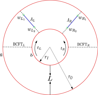
Figure 16: This schematic depicts a generic subsystem ($A=A_{L}\cup A_{R}$) with both the end points in the bulk of $BCFT_{L}$ and $BCFT_{R}$ at a constant time slice. (Figure modified from Geng:2021iyq )

$\bm{(c)}$ A similar computation of the entanglement entropy may be performed by considering the BOEs of all the twist operators with respect to the other boundary located at the operator insertion point $z=\frac{i}{2}$ on the UHP. Hence the corresponding entanglement entropy in this disconnected channel may be obtained on the $w$-plane as,

$$S^{aa}_{A}= \lim_{n\rightarrow 1}\frac{1}{1-n}\log\Big{(}\left<\Phi_{n}\left(z_{R_{1}},\bar{z}_{R_{1}}\right)\bar{\Phi}_{n}\left(z_{L_{1}},\bar{z}_{L_{1}}\right)\Phi_{n}\left(z_{R_{2}},\bar{z}_{R_{2}}\right)\bar{\Phi}_{n}\left(z_{L_{2}},\bar{z}_{L_{2}}\right)\Phi_{a}\left(z_{a},\bar{z}_{a}\right)\right>_{\text{UHP}}\Big{)}$$

$$= \frac{c}{3}\ln\left(\frac{r_{O}^{2}-r_{1}^{2}}{r_{O}\epsilon}\right)+\frac{c}{3}\ln\left(\frac{r_{O}^{2}-r_{2}^{2}}{r_{O}\epsilon}\right)+4\ln\left(g_{a}\right)\,.$$ (33)

$\bm{(d)}$ Now we discuss the case where both the OPE and the BOE of the twist operators may be considered simultaneously. The entanglement entropy in this connected channel may be written as

$$S^{b\text{-bulk}}_{A}= \lim_{n\rightarrow 1}\frac{1}{1-n}\log(\left<\bar{\Phi}_{n}\left(z_{L_{1}},\bar{z}_{L_{1}}\right)\Phi_{n}\left(z_{R_{1}},\bar{z}_{R_{1}}\right)\right>^{b}_{\text{UHP}}\left<\bar{\Phi}_{n}\left(z_{R_{2}},\bar{z}_{R_{2}}\right)\Phi_{n}\left(z_{L_{2}},\bar{z}_{L_{2}}\right)\right>_{\text{UHP}})$$

$$= \frac{c}{3}\ln\left(\frac{2r_{2}}{\epsilon}\cosh\frac{2\pi t}{\beta}\right)+\frac{c}{3}\ln\left(\frac{r_{1}^{2}-r_{I}^{2}}{r_{I}\epsilon}\right)+2\ln\left(g_{b}\right)\,,$$ (34)

where we have performed BOEs for the twist operators $\Phi_{n}\left(z_{R_{1}},\bar{z}_{R_{1}}\right)\,,\,\bar{\Phi}_{n}\left(z_{L_{1}},\bar{z}_{L_{1}}\right)$ and considered the OPE of the rest $\bar{\Phi}_{n}\left(z_{R_{2}},\bar{z}_{R_{2}}\right)\,,\,\Phi_{n}\left(z_{L_{2}},\bar{z}_{L_{2}}\right)$ on the UHP. Once again, in the last line we have utilized the transformations $w_{L}=r\exp(i\theta)\,,\,w_{R}=r\exp(i\pi-i\theta)$ followed by an analytic continuation of the Euclidean time $t=\frac{i\theta\beta}{2\pi}$ on the $w$-plane.

$\bm{(e)}$ Conversely we may employ the OPE of the twist operators $\Phi_{n}\left(z_{R_{1}},\bar{z}_{R_{1}}\right)\,,\,\bar{\Phi}_{n}\left(z_{L_{1}},\bar{z}_{L_{1}}\right)$ and BOEs to the remaining twist operators, resulting into an another possibility of the entanglement entropy in the connected channel as follows

$$S^{a\text{-bulk}}_{A}= \lim_{n\rightarrow 1}\frac{1}{1-n}\log\Big{(}\left<\bar{\Phi}_{n}\left(z_{L_{1}},\bar{z}_{L_{1}}\right)\Phi_{n}\left(z_{R_{1}},\bar{z}_{R_{1}}\right)\right>_{\text{UHP}}$$

$$\qquad\qquad\qquad\left<\bar{\Phi}_{n}\left(z_{R_{2}},\bar{z}_{R_{2}}\right)\Phi_{n}\left(z_{L_{2}},\bar{z}_{L_{2}}\right)\Phi_{a}\left(z_{a},\bar{z}_{a}\right)\right>_{\text{UHP}}\Big{)}$$

$$= \frac{c}{3}\ln\left(\frac{2r_{1}}{\epsilon}\cosh\frac{2\pi t}{\beta}\right)+\frac{c}{3}\ln\left(\frac{r_{O}^{2}-r_{2}^{2}}{r_{I}\epsilon}\right)+2\ln\left(g_{a}\right)\,.$$ (35)

Note that, we have performed the corresponding BOEs in the above equation with respect to the boundary $a$.

$\bm{(f)}$ An another case may also be analyzed by considering the BOEs of the twist operators involving both the boundaries on the UHP simultaneously. Hence, the entanglement entropy corresponding to this connected channel may be reduced to

$$\begin{split}S^{ab}_{A}=&\lim_{n\rightarrow 1}\frac{1}{1-n}\log\Big{(}\left<\bar{\Phi}_{n}\left(z_{L_{1}},\bar{z}_{L_{1}}\right)\Phi_{n}\left(z_{R_{1}},\bar{z}_{R_{1}}\right)\right>^{b}_{\text{UHP}}\Big{.}\\ &\Big{.}~{}~{}~{}~{}~{}~{}~{}~{}~{}~{}~{}~{}~{}~{}~{}~{}~{}\left<\bar{\Phi}_{n}\left(z_{R_{2}},\bar{z}_{R_{2}}\right)\Phi_{n}\left(z_{L_{2}},\bar{z}_{L_{2}}\right)\Phi_{a}\left(z_{a},\bar{z}_{a}\right)\right>_{\text{UHP}}\Big{)}\,\\ =&\frac{c}{3}\ln\left(\frac{r_{1}^{2}-r_{I}^{2}}{r_{I}\epsilon}\right)+\frac{c}{3}\ln\left(\frac{r_{O}^{2}-r_{2}^{2}}{r_{I}\epsilon}\right)+2\ln\left(g_{a}\right)+2\ln\left(g_{b}\right)\,.\end{split}$$ (36)

$\bm{(g)}$ We now discuss a special case of the disconnected channels where the contribution to the entanglement entropy may be computed from the OPE of the twist operators $\bar{\Phi}_{n}\left(w_{L_{1}},\bar{w}_{L_{1}}\right)$, $\Phi_{n}\left(w_{L_{2}},\bar{w}_{L_{2}}\right)$ in the $BCFT_{L}$ and similarly for $\bar{\Phi}_{n}\left(w_{R_{1}},\bar{w}_{R_{1}}\right)$, $\Phi_{n}\left(w_{R_{2}},\bar{w}_{R_{2}}\right)$ in the $BCFT_{R}$ . The expression for the entanglement entropy in this channel is then given as

$$S^{\text{dome}}_{A}= \lim_{n\rightarrow 1}\frac{1}{1-n}\log\Big{(}\left<\bar{\Phi}_{n}\left(z_{L_{1}},\bar{z}_{L_{1}}\right)\Phi_{n}\left(z_{L_{2}},\bar{z}_{L_{2}}\right)\right>_{\text{UHP}}\left<\Phi_{n}\left(z_{R_{1}},\bar{z}_{R_{1}}\right)\bar{\Phi}_{n}\left(z_{R_{2}},\bar{z}_{R_{2}}\right)\right>_{\text{UHP}}\Big{)}$$

$$= \frac{c}{3}\ln\left(\frac{\beta}{\pi\epsilon}\sinh\frac{\pi(r_{2}-r_{1})}{\beta}\right)\,.$$ (37)

Finally, the entanglement entropy of a generic subsystem $A$ may be obtained by considering the minimum of the above contributions.

$$S_{A}=\text{min}\left(S^{\text{bulk}}_{A},S^{bb}_{A},S^{aa}_{A},S^{b\text{-bulk}}_{A},S^{a\text{-bulk}}_{A},S^{ab}_{A},S^{\text{dome}}_{A}\right)\,.$$ (38)

In the following subsection, we will compute the corresponding entanglement entropy from the dual bulk geometry through wedge holography which will substantiate the above field theory results.

A.1.2 Holographic computations

We now compute the holographic entanglement entropy for a generic subsystem $A$ at a finite temperature using the areas of the RT surfaces described in Geng:2021iyq for the bulk dual geometry involving an eternal $AdS_{3}$ BTZ black hole with two dimensional KR branes Geng:2021iyq . Once more it is possible to identify seven contributions to the entanglement entropy of the subsystem $A$ arising from distinct bulk RT surfaces. In what follows we describe the areas of these various RT surfaces for the subsystem $A$ as mentioned above. In this context we have considered both the asymptotic regions of the bulk BTZ geometry for computing the areas of the corresponding RT surfaces in contrast to Geng:2021iyq where only a single asymptotic region was considered and finally the authors doubled the results to obtain the areas of the RT surfaces.

$\bm{(a)}$ We start with the RT surfaces for the subsystem $A$ which consists of two HM surfaces connecting its end points in the two asymptotic boundaries as illustrated in the fig. 17(a). We call this RT surface as bulk-type with an area contribution as follows

$$A_{\text{bulk}}=2\ln\left(\frac{2r_{1}}{\epsilon}\cosh\frac{2\pi t}{\beta}\right)+2\ln\left(\frac{2r_{2}}{\epsilon}\cosh\frac{2\pi t}{\beta}\right)\,.$$ (39)

$\bm{(b)}$ Next we consider the $bb$-type RT surfaces where both the geodesics start from $\partial A$ and end on the $b$-brane as shown in the fig. 17(b). The corresponding area contribution may be obtained as

$$A_{bb}=2\ln\left(\frac{r_{1}^{2}-r_{I}^{2}}{r_{I}\epsilon}\right)+2\ln\left(\frac{r_{2}^{2}-r_{I}^{2}}{r_{I}\epsilon}\right)+4\frac{6}{c}\ln\left(g_{b}\right)\,.$$ (40)

$\bm{(c)}$ Similar to above case, if both the geodesics start from $\partial A$ and end on the $a$-brane, they are termed as the $aa$-type RT surfaces as described in fig. 17(c). The area for these RT surfaces is given by

$$A_{aa}=2\ln\left(\frac{r_{O}^{2}-r_{1}^{2}}{r_{O}\epsilon}\right)+2\ln\left(\frac{r_{O}^{2}-r_{2}^{2}}{r_{O}\epsilon}\right)+4\frac{6}{c}\ln\left(g_{a}\right)\,.$$ (41)

$\bm{(d)}$ Next we describe the contribution to the EE of the subsystem $A$ from $b$-bulk type RT surfaces (fig. 17(d)) where both the geodesics start from $\partial A$, however two of them end on the $b$-brane while the other geodesic stretches between the two asymptotic boundaries as a HM surface. The area for this contribution is expressed as

$$A_{\text{$b$-bulk}}=2\ln\left(\frac{2r_{2}}{\epsilon}\cosh\frac{2\pi t}{\beta}\right)+2\ln\left(\frac{r_{1}^{2}-r_{I}^{2}}{r_{I}\epsilon}\right)+2\frac{6}{c}\ln\left(g_{b}\right)\,.$$ (42)

$\bm{(e)}$ These RT surfaces are similar to the previous one but with the geodesics now ending on the $a$-brane instead of the $b$-brane (fig. 17(e)). We term these RT surfaces as $a$-bulk type with an area

$$A_{\text{$a$-bulk}}=2\ln\left(\frac{2r_{1}}{\epsilon}\cosh\frac{2\pi t}{\beta}\right)+2\ln\left(\frac{r_{O}^{2}-r_{2}^{2}}{r_{I}\epsilon}\right)+2\frac{6}{c}\ln\left(g_{a}\right)\,.$$ (43)

$\bm{(f)}$ We now consider the $ab$-type RT surfaces where the geodesics start from $\partial A$ and end on the two KR branes as depicted in the fig. 17(f) with an area contribution as follows

$$A_{ab}=2\ln\left(\frac{r_{1}^{2}-r_{I}^{2}}{r_{I}\epsilon}\right)+2\ln\left(\frac{r_{O}^{2}-r_{2}^{2}}{r_{I}\epsilon}\right)+2\frac{6}{c}\ln\left(g_{a}\right)+2\frac{6}{c}\ln\left(g_{b}\right)\,.$$ (44)

$\bm{(g)}$ Finally, we have the dome-type RT surfaces described by the geodesics homologous to the subsystem $A$ on both the asymptotic boundaries (fig. 17(g)). At finite temperature this configuration describes an area contribution to the EE given by

$$A_{\text{dome}}=4\ln\left(\frac{\beta}{\pi\epsilon}\sinh\frac{\pi(r_{2}-r_{1})}{\beta}\right)\,.$$ (45)

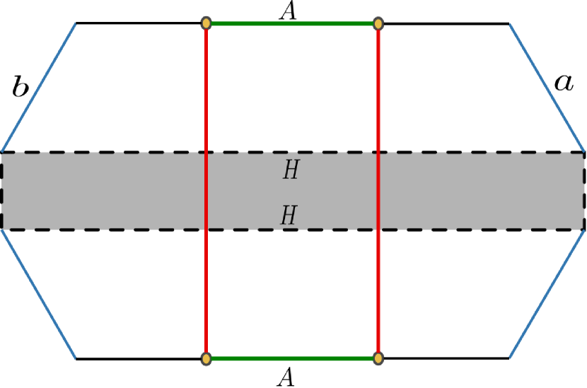
(a)

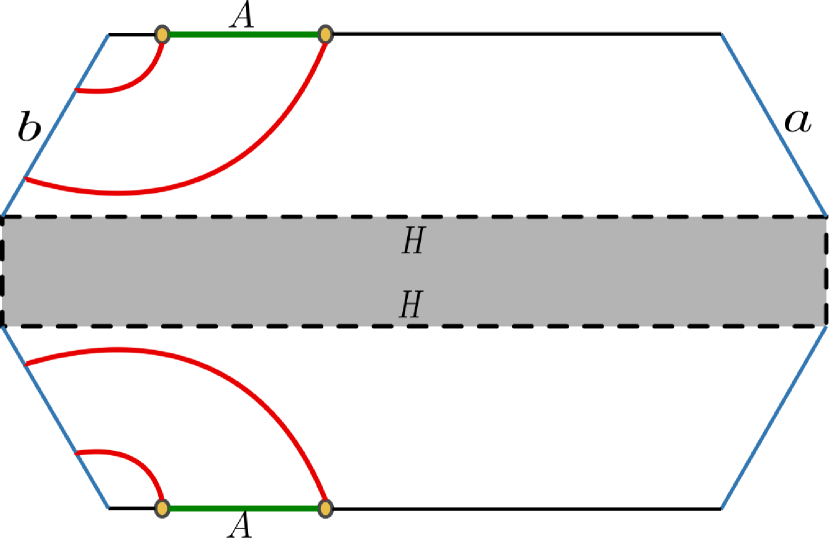
(b)

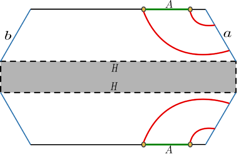
(c)

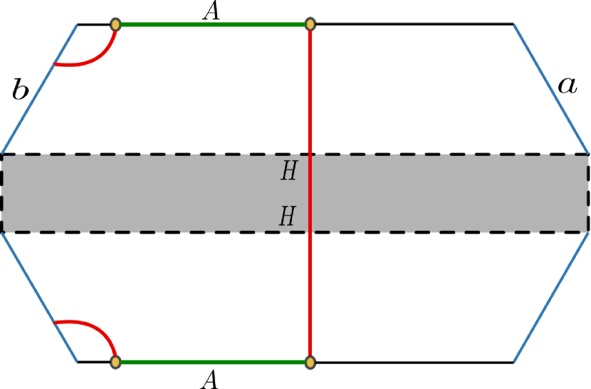
(d)

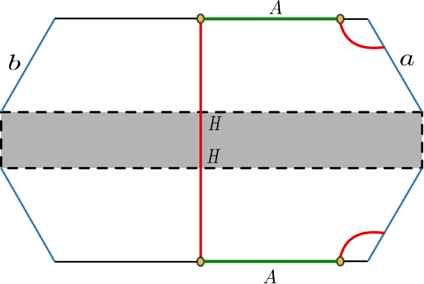
(e)

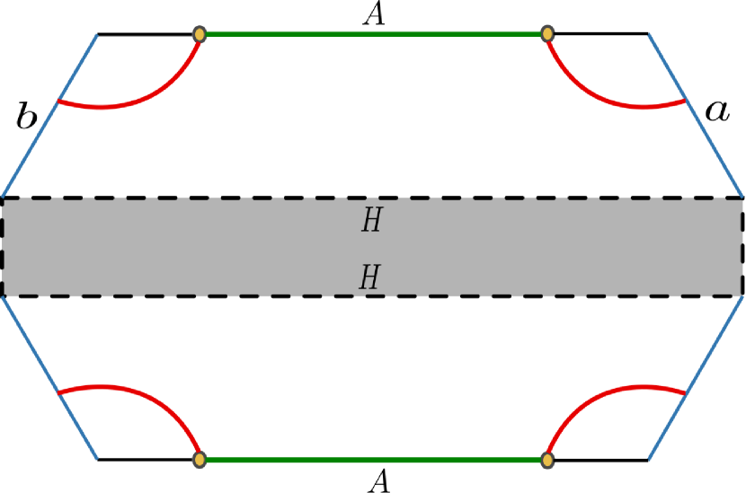
(f)

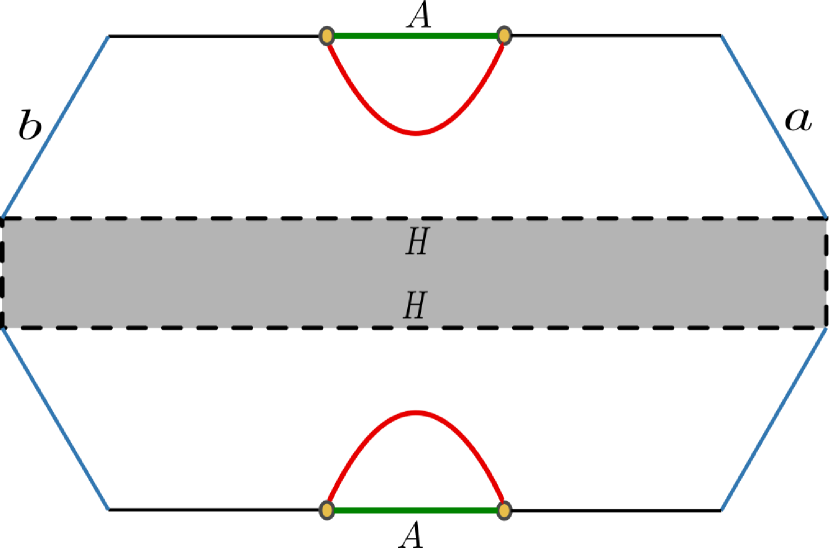
(g)

Figure 17: Diagram depicts all the possible RT surfaces corresponding to the subsystem $A$. Here the two asymptotic boundaries and the horizons of the bulk eternal BTZ black hole are denoted by the black solid lines and the grey shaded region respectively whereas the two KR branes are shown by the blue lines labeled as $a$ and $b$ corresponding to the different boundary conditions of the dual $BCFT_{2}$s. (Figure modified from Geng:2021hlu ; Geng:2021iyq )

Now we may compute the holographic entanglement entropy for the subsystem $A$ in the dual $BCFT_{2}$s by utilizing the wedge holography relation discussed in eq. (4.4) of Geng:2021iyq and eqs. 41, 40, 44, 39, 43, 42 and 45

$$S_{A}= \text{min}\left(\frac{A_{\text{bulk}}}{4G_{N}^{(3)}},\frac{A_{bb}}{4G_{N}^{(3)}},\frac{A_{aa}}{4G_{N}^{(3)}},\frac{A_{b\text{-bulk}}}{4G_{N}^{(3)}},\frac{A_{a\text{-bulk}}}{4G_{N}^{(3)}},\frac{A_{ab}}{4G_{N}^{(3)}},\frac{A_{dome}}{4G_{N}^{(3)}}\right)\,$$ (46)

$$= \text{min}\left(S^{\text{bulk}}_{A},S^{bb}_{A},S^{aa}_{A},S^{b\text{-bulk}}_{A},S^{a\text{-bulk}}_{A},S^{ab}_{A},S^{\text{dome}}_{A}\right)\,.$$

In the following, we plot the entanglement entropies corresponding to the RT surfaces detailed above with respect to the size of the subsystem $A$ and time $t$.

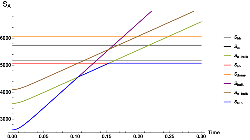
(a) Entanglement entropies corresponding to the different RT surfaces w.r.t time. Here $A=[1.01,1.5]$ and time $t$ is varied from [0, .3]

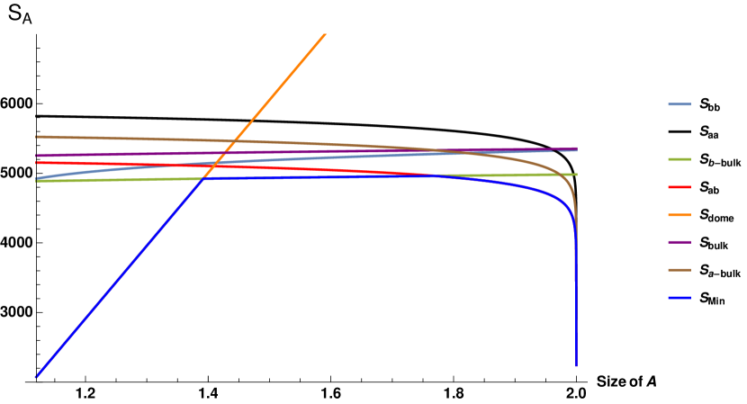
(b) Entanglement entropies corresponding to the different RT surfaces w.r.t the size of the subsystem $A$. Here $t=.15$ and the size of $A$ is varied from $[1.01+\epsilon,r_{O}-\epsilon]$.

Figure 18: In the above figures, we have chosen $\beta=.1$, $c=500$, $\epsilon=.001$, $r_{I}=1$, $r_{O}=2$, $S_{bdyb}=875$, $S_{bdya}=850$.

A.2 Holographic entanglement negativity and Page curve

In this subsection we compute the holographic entanglement negativity for various bipartite mixed states in the context of the braneworld model-II from the proposals described in eqs. 20 and 25 and the expression for the holographic entanglement entropy in eq. 46. Subsequently we study the characteristics of the holographic entanglement negativity obtained for different scenarios involving the subsystem sizes and the time for this configuration. Some of these profiles describe the corresponding Page curves for the holographic entanglement negativity. It is important to note here that the first Page curve was obtained in the context of a bipartite quantum system in Page:1993df using the Harr random average of the entanglement entropy for one of the subsystem as a function of the size of its Hilbert space. This Page curve was later interpreted in the context of black hole systems as the evolution of the EE for the Hawking radiation with respect to the time Page:1993wv ; Page:2013dx . Recently, the Page curves for the entanglement negativity of bipartite mixed states were obtained through the random matrix techniques in Shapourian:2020mkc . Interestingly the corresponding Page curves for the entanglement negativity obtained through our holographic constructions for the configuration of two communicating black holes Geng:2021iyq considered here are similar in nature.

A.2.1 Adjacent subsystems

In this subsection, we compute the holographic entanglement negativity for two generic adjacent subsystems $A$ and $B$ in the dual $BCFT_{2}$s by utilizing the eqs. 20 and 46. In particular, we investigate the qualitative nature of the entanglement negativity and discuss its profiles for three distinct scenarios involving the subsystem sizes and the time in the first model. In this context, we use the diagrams similar to those depicted in fig. 17 to study the various RT surfaces for the two adjacent subsystems under consideration.

$\bm{(i)}$ Full system ($\bm{A\cup B}$) fixed, common point varied

In the first case, we obtain the profile for the entanglement negativity between two adjacent subsystems $A=[r_{I}+\epsilon,r]$ and $B=[r,r_{O}-\epsilon]$ at a constant time slice while varying the common point $r$ as shown in fig. 19(a). We compute the holographic entanglement negativity between $A$ and $B$ using the eqs. 46 and 20 as follows

$$\mathcal{E}(A:B)=\begin{cases}\frac{c}{4}\log\left[\frac{\beta^{2}(r-r_{I})(r+r_{I})\sinh^{2}\left(\frac{\pi(r-r_{I}-\epsilon)}{\beta}\right)}{\pi^{2}\epsilon^{3}(2r_{I}+\epsilon)}\right]\,,&\text{Phase-1}\vspace{2mm}\\ \frac{c}{4}\log\left[\frac{2\beta^{2}rr_{I}\cosh\left(\frac{2\pi t}{\beta}\right)\sinh^{2}\left(\frac{\pi(r-r_{I}-\epsilon)}{\beta}\right)}{\pi^{2}\epsilon^{3}(2r_{I}+\epsilon)}\right]-2S_{\text{bdyb}}\,,&\text{Phase-2}\vspace{2mm}\\ \frac{c}{4}\log\left[\frac{4r^{2}\cosh^{2}\left(\frac{2\pi t}{\beta}\right)}{\epsilon^{2}}\right]\,,&\text{Phase-3}\vspace{2mm}\\ \frac{c}{4}\log\left[\frac{(r_{O}-r)^{2}(r+r_{O})^{2}}{r_{O}^{2}\epsilon^{2}}\right]+4S_{\text{bdya}}\,,&\text{Phase-4}\vspace{2mm}\\ \frac{c}{4}\log\left[\frac{\beta^{2}(r_{O}-r)(r+r_{O})\sinh^{2}\left(\frac{\pi(r-r_{O}+\epsilon)}{\beta}\right)}{\pi^{2}\epsilon^{3}(2r_{O}-\epsilon)}\right]\,,&\text{Phase-5}\end{cases}$$ (47)

where the boundary entropies corresponding to the two KR branes are denoted as $S_{\text{bdya}}$ and $S_{\text{bdyb}}$. It is interesting to note that the behaviour of the Page curve for the entanglement negativity in this context is analogous to the one obtained in KumarBasak:2021rrx ; Shapourian:2020mkc .

In the present scenario, we identify all the possible contributions to the entanglement entropies of the subsystems $A$ and $B$ by using eq. 46 to elucidate the phase transitions observed in fig. 19(a). In this context it is possible to identify five distinct phases for the holographic entanglement negativity between the two adjacent subsystems which is described as follows.

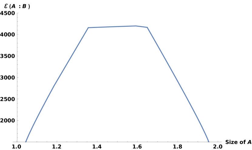
(a) Page curve for the entanglement negativity with respect to the size of the subsystem $A$.

(b) The entanglement negativity between the adjacent subsystems as a function of the size of $B$ where $r_{1}=1.15$.

Figure 19: Here $r_{I}=1$, $r_{O}=2$, $\epsilon=.001$, $\beta=.1$, $c=500$, $t=.15$, $S_{bdyb}=875$ and $S_{bdya}=850$.

$\bm{(ii)}$ Subsystem $\bm{A}$ fixed, $\bm{B}$ varied

Next we analyze the behaviour of the entanglement negativity between the two adjacent subsystems at a constant time slice where we consider the subsystem $A=[r_{I}+\epsilon,r_{1}]$ with a fixed size and vary the size of the subsystem $B=[r_{1}+\epsilon,r]$ by shifting the point $r$. This is obtained by using the eqs. 46 and 20 as follows

$$\mathcal{E}(A:B)=\begin{cases}\frac{c}{2}\log\left[\frac{\beta\sinh\left(\frac{\pi\left(r_{1}-r\right)}{\beta}\right)\sinh\left(\frac{\pi\left(-r_{1}+r_{I}+\epsilon\right)}{\beta}\right)\text{csch}\left(\frac{\pi(r-r_{I}-\epsilon)}{\beta}\right)}{\pi\epsilon}\right]\,,&\text{Phase-1}\vspace{2mm}\\ \frac{c}{4}\log\left[\frac{\beta^{4}r_{I}\text{sech}\left(\frac{2\pi t}{\beta}\right)\sinh^{2}\left(\frac{\pi\left(r-r_{1}\right)}{\beta}\right)\sinh^{2}\left(\frac{\pi\left(-r_{1}+r_{I}+\epsilon\right)}{\beta}\right)}{2\pi^{4}r\epsilon^{3}(2r_{I}+\epsilon)}\right]+2S_{\text{bdyb}}\,,&\text{Phase-2}\vspace{2mm}\\ \frac{c}{4}\log\left[\frac{\beta^{2}\left(r_{1}^{2}-r_{I}^{2}\right)\sinh^{2}\left(\frac{\pi\left(-r_{1}+r_{I}+\epsilon\right)}{\beta}\right)}{\pi^{2}\epsilon^{3}(2r_{I}+\epsilon)}\right]\,,&\text{Phase-3}\end{cases}$$ (48)

which corresponds to three possible phases for the entanglement negativity between $A$ and $B$ as depicted in fig. 19(b). In what follows we analyze these phases in detail.

$\bm{(iii)}$ Subsystems $\bm{A}$ and $\bm{B}$ fixed, time varied

Finally we investigate the holographic entanglement negativity between the adjacent subsystems $A$ and $B$ with fixed lengths $l_{1}$ and $l_{2}$ respectively while varying the time. In particular, we will study two sub cases of equal and unequal lengths of the two subsystems in question and obtain the corresponding entanglement negativities as depicted in the fig. 20.

Figure 20: Page curves for the entanglement negativity between two adjacent subsystems $A$ and $B$ as a function of time. Here $r_{I}=1$, $r_{O}=2$, $\epsilon=.001$, $\beta=.1$, $c=500$, $S_{bdyb}=875$, $S_{bdya}=850$ and $A=[r_{I}+\epsilon,r_{1}]$, $B=[r_{1},r_{O}-\epsilon]$ with $r_{1}=1.5$ (for $l_{1}=l_{2}$) and $A=[r_{I}+\epsilon,r_{1}]$, $B=[r_{1},r_{O}-\epsilon]$ with $r_{1}=1.3$ (for $l_{1}\neq l_{2}$).

(a) For $\bm{l_{1}=l_{2}}$
For the case of two equal length subsystems $A$ and $B$, we observe two phases in the entanglement negativity profile as depicted in fig. 20. The expressions for these may be obtained by utilizing the eqs. 46 and 20 as follows

$$\mathcal{E}(A:B)=\begin{cases}\frac{c}{4}\log\left[\frac{4r_{1}^{2}\cosh^{2}\left(\frac{2\pi t}{\beta}\right)}{\epsilon^{2}}\right]\,,&\text{Phase-1}\vspace{3mm}\\ \frac{c}{4}\log\left[\frac{\left(r_{O}^{2}-r_{1}^{2}\right)^{2}}{r_{O}^{2}\epsilon^{2}}\right]+4S_{\text{bdya}}\,.&\text{Phase-2}\end{cases}$$ (49)

(b) For $\bm{l_{1}\neq l_{2}}$
Here we consider two unequal lengths of the subsystems $A$ and $B$ and compute the holographic entanglement negativity between them utilizing the eqs. 46 and 20. We observe three consecutive phases in the entanglement negativity profile as depicted in fig. 20. The expressions for the corresponding entanglement negativity in these phases are given as follows

$$\mathcal{E}(A:B)=\begin{cases}\frac{c}{4}\log\left[\frac{4r_{1}^{2}\cosh^{2}\left(\frac{2\pi t}{\beta}\right)}{\epsilon^{2}}\right]\,,&\text{Phase-1}\vspace{2mm}\\ \frac{c}{4}\log\left[\frac{2\beta^{2}r_{1}r_{I}\cosh\left(\frac{2\pi t}{\beta}\right)\sinh^{2}\left(\frac{\pi\left(-r_{1}+r_{I}+\epsilon\right)}{\beta}\right)}{\pi^{2}\epsilon^{3}(2r_{I}+\epsilon)}\right]-2S_{\text{bdyb}}\,\,,&\text{Phase-2}\vspace{2mm}\\ \frac{c}{4}\log\left[\frac{\beta^{2}\left(r_{1}^{2}-r_{I}^{2}\right)\sinh^{2}\left(\frac{\pi\left(-r_{1}+r_{I}+\epsilon\right)}{\beta}\right)}{\pi^{2}\epsilon^{3}(2r_{I}+\epsilon)}\right]\,.&\text{Phase-3}\end{cases}$$ (50)

A.2.2 Disjoint subsystems

Now we consider two generic disjoint subsystems $A$ and $B$ with a subsystem $C$ enclosed between them in the dual $BCFT_{2}$s and compute the holographic entanglement negativity between $A$ and $B$ using the eqs. 25 and 46. In particular, we will investigate the qualitative feature of the entanglement negativity profile for three different scenarios of the disjoint subsystems involving the subsystem sizes and the time in the context of the braneworld model-II. Once again we utilize diagrams similar to those depicted in fig. 17 to study the various RT surfaces for the subsystems in question.

$\bm{(i)}$ Subsystem $\bm{A}$ fixed, $\bm{C}$ varied

In the first case, we fix the size of the subsystem $A=[r_{I}+\epsilon,r_{1}]$ at a constant time slice and vary the size of $C=[r_{1},r]$ by shifting the point $r$ from $r_{1}+\epsilon$ to $r_{O}-\epsilon$ to examine the holographic entanglement negativity between the subsystems $A$ and $B$. To this end, we may compute the entanglement negativity by utilizing the eqs. 25 and 46 as follows

$$\mathcal{E}(A:B)=\begin{cases}\frac{c}{4}\log\left[\frac{\left(-r_{I}^{2}+r_{1}^{2}\right)\sinh^{2}\left(\frac{\pi\left(r-r_{I}-\epsilon\right)}{\beta}\right)}{\epsilon(2r_{I}+\epsilon)\sinh^{2}\left(\frac{\pi\left(r-r_{1}\right)}{\beta}\right)}\right]\;,&\text{Phase-1}\vspace{3mm}\\ \frac{c}{4}\log\left[\frac{2\pi^{2}\,r\,\left(-r_{I}^{2}+r_{1}^{2}\right)\cosh\left(\frac{2\pi t}{\beta}\right)}{\beta^{2}r_{I}\epsilon\sinh^{2}\left(\frac{\pi\left(r-r_{1}\right)}{\beta}\right)}\right]+2S_{\text{bdyb}}\;\;,&\text{Phase-2}\vspace{3mm}\\ 0\;.&\text{Phase-3}\end{cases}$$ (51)

Here we observe three phases from the corresponding entanglement negativity profile as depicted in fig. 21(a) which we now analyze in details.

(a) Entanglement negativity between two disjoint subsystems with the variation of size $C$ where $r_{1}=1.15$.

(b) The entanglement negativity between two disjoint subsystems $A\,\text{and}\,B$ with a variation in the size of $B$ where $r_{1}=1.15$ and $r_{2}=1.25$.

Figure 21: Here, $r_{I}=1$, $r_{O}=2$, $\epsilon=.001$, $\beta=.1$, $c=500$, $t=.15$, $S_{bdyb}=875$, $S_{bdya}=850$.

$\bm{(ii)}$ Subsystems $\bm{A}$ and $\bm{C}$ fixed, $\bm{B}$ varied

In this case, we consider the subsystem sizes of $A=[r_{I}+\epsilon,r_{1}]$ and $C=[r_{1},r_{2}]$ to be fixed and vary the size of $B=[r_{2}+\epsilon,r]$ by shifting the point $r$. The entanglement negativity between the two disjoint subsystems $A$ and $B$ corresponds to three consecutive phases as shown in fig. 21(b). In this context, the size of $C$ is considered to be very small such that the dominant contribution to its entanglement entropy arises from dome-type RT surfaces throughout this case. Finally, the expressions for the entanglement negativity in this scenario may be given as

$$\mathcal{E}(A:B)=\begin{cases}\frac{c}{2}\log\left[\frac{\sinh\left(\frac{\pi\left(-r_{1}+r\right)}{\beta}\right)\sinh\left(\frac{\pi\left(-r_{2}+r_{I}+\epsilon\right)}{\beta}\right)}{\sinh\left(\frac{\pi\left(r_{1}-r_{2}\right)}{\beta}\right)\sinh\left(\frac{\pi\left(r-r_{I}-\epsilon\right)}{\beta}\right)}\right]\;,&\text{Phase-1}\vspace{2mm}\\ \frac{c}{4}\log\left[\frac{\beta^{2}r_{I}\text{sech}\left(\frac{2\pi t}{\beta}\right)\sinh^{2}\left(\frac{\pi\left(-r_{1}+r\right)}{\beta}\right)\sinh^{2}\left(\frac{\pi\left(-r_{2}+r_{I}+\epsilon\right)}{\beta}\right)}{2\pi^{2}\epsilon\,r\,(2r_{I}+\epsilon)\sinh^{2}\left(\frac{\pi\left(r_{1}-r_{2}\right)}{\beta}\right)}\right]-2S_{\text{bdyb}}\;\;,&\text{Phase-2}\vspace{2mm}\\ \frac{c}{4}\log\left[\frac{\left(r_{1}^{2}-r_{I}^{2}\right)\sinh^{2}\left(\frac{\pi\left(-r_{2}+r_{I}+\epsilon\right)}{\beta}\right)}{\epsilon(2r_{I}+\epsilon)\sinh^{2}\left(\frac{\pi\left(r_{1}-r_{2}\right)}{\beta}\right)}\right]\;.&\text{Phase-3}\end{cases}$$ (52)

Note that in the present scenario, we increase only the size of the subsystem $B$ at a constant time slice while fixing the size of $A$ and $C$. This is similar to the adjacent case discussed in subsection A.2 where we have fixed the size of the subsystem $A$ and increased the size of $B$. Hence all the above phases may be described in terms of the Hawking modes using the explanations analogous to the adjacent case.

$\bm{(iii)}$ Subsystems $\bm{A}$, $\bm{B}$ and $\bm{C}$ fixed, time varied

We end our analysis with the final case where we investigate the nature of the entanglement negativity between the two disjoint subsystems $A$ and $B$ with lengths $l_{1}$ and $l_{2}$ respectively while varying the time. Here we consider the size of the subsystem $C$ to be very small such that the dominant contribution to the entanglement entropy arises from dome-type RT surfaces. Note that, the entanglement wedges of the subsystems $A$ and $B$ are connected in this scenario which corresponds to a non-zero entanglement negativity between them. In what follows, we explore two sub cases of equal and unequal lengths of the subsystems $A$ and $B$ while varying the time.

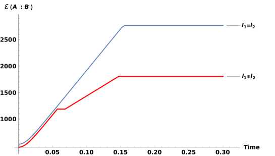
Figure 22: The Page curves for the entanglement negativity for two disjoint subsystems as a function of time. In this case we have chosen $r_{I}=1$, $r_{O}=2$, $\epsilon=.001$, $\beta=.1$, $c=500$, $S_{bdyb}=875$, $S_{bdya}=850$ and $A=[r_{I}+\epsilon,r_{1}]$, $B=[r_{2},r_{O}-\epsilon]$ with $r_{1}=1.45$, $r_{2}=1.55$ (for $l_{1}=l_{2}$) and $A=[r_{I}+\epsilon,r_{1}]$, $B=[r_{2},r_{O}-\epsilon]$ with $r_{1}=1.15$, $r_{2}=1.25$ (for $l_{1}\neq l_{2}$).

(a) For $\bm{l_{1}=l_{2}}$

For the case of two equal length subsystems $A$ and $B$, we examine the qualitative profile of the entanglement negativity between them which corresponds to three different phases as depicted in fig. 22. In this context, we may compute the entanglement negativity by utilizing eqs. 25 and 46 as follows

$$\mathcal{E}(A:B)=\begin{cases}\frac{c}{4}\log\left[\frac{4\pi^{2}r_{1}\,r_{2}\,\cosh^{2}\left(\frac{2\pi t}{\beta}\right)}{\beta^{2}\sinh^{2}\left(\frac{\pi\left(r_{1}-r_{2}\right)}{\beta}\right)}\right]\,,&\text{Phase-1}\vspace{2mm}\\ \frac{c}{4}\log\left[\frac{2\pi^{2}r_{2}\left(r_{1}^{2}-r_{I}^{2}\right)\cosh\left(\frac{2\pi t}{\beta}\right)}{\beta^{2}r_{I}\sinh^{2}\left(\frac{\pi\left(r_{1}-r_{2}\right)}{\beta}\right)}\right]+2S_{\text{bdyb}}\,\,,&\text{Phase-2}\vspace{2mm}\\ \frac{c}{4}\log\left[\frac{\pi^{2}\left(r_{1}^{2}-r_{I}^{2}\right)\left(r_{O}^{2}-r_{2}^{2}\right)}{\beta^{2}r_{I}\,\,r_{O}\sinh^{2}\left(\frac{\pi\left(r_{1}-r_{2}\right)}{\beta}\right)}\right]+2S_{\text{bdyb}}+2S_{\text{bdya}}\,\,.&\text{Phase-3}\\ \end{cases}$$ (53)

(b) For $\bm{l_{1}\neq l_{2}}$

Finally we consider two disjoint subsystems $A$ and $B$ with unequal lengths while increasing the time and compute the entanglement negativity between them utilizing eqs. 25 and 46. In this context, we obtain four consecutive phases of the corresponding entanglement negativity profile which may be expressed as follows

$$\mathcal{E}(A:B)=\begin{cases}\frac{c}{4}\log\left[\frac{4\pi^{2}r_{1}\,r_{2}\,\cosh^{2}\left(\frac{2\pi t}{\beta}\right)}{\beta^{2}\sinh^{2}\left(\frac{\pi\left(r_{1}-r_{2}\right)}{\beta}\right)}\right]\,,&\text{Phase-1}\vspace{2mm}\\ \frac{c}{4}\log\left[\frac{r_{O}(r_{O}-\epsilon)\left(-r_{I}^{2}+r_{1}^{2}\right)\sinh^{2}\left(\frac{\pi\left(-r_{2}+r_{I}+\epsilon\right)}{\beta}\right)}{r_{I}\epsilon(r_{I}+\epsilon)(2r_{O}-\epsilon)\sinh^{2}\left(\frac{\pi\left(r_{1}-r_{2}\right)}{\beta}\right)}\right]-2S_{\text{bdya}}+2S_{\text{bdyb}}\,,&\text{Phase-2}\vspace{2mm}\\ \frac{c}{4}\log\left[\frac{2r_{O}(r_{O}-\epsilon)\left(-r_{I}^{2}+r_{1}^{2}\right)\sinh^{2}\left(\frac{\pi\left(-r_{2}+r_{I}+\epsilon\right)}{\beta}\right)\cosh\left(\frac{2\pi t}{\beta}\right)}{r_{I}\epsilon^{2}(2r_{I}+\epsilon)(2r_{O}-\epsilon)\sinh^{2}\left(\frac{\pi\left(r_{1}-r_{2}\right)}{\beta}\right)}\right]-2S_{\text{bdya}}\,\,,&\text{Phase-3}\vspace{2mm}\\ \frac{c}{4}\log\left[\frac{\left(r_{1}^{2}-r_{I}^{2}\right)\sinh^{2}\left(\frac{\pi\left(-r_{2}+r_{I}+\epsilon\right)}{\beta}\right)}{\epsilon(2r_{I}+\epsilon)\sinh^{2}\left(\frac{\pi\left(r_{1}-r_{2}\right)}{\beta}\right)}\right]\,\,.&\text{Phase-4}\end{cases}$$ (54)

Appendix B Expressions for holographic entanglement negativity for braneworld model

In this appendix, we show the expressions for the holographic entanglement negativity between two adjacent and disjoint subsystems obtained through the eqs. 20, 25 and 15 in the braneworld model.

Adjacent subsystems

Here we list the expressions of the holographic entanglement negativity between two adjacent subsystems utilizing the eqs. 20 and 15 in three distinct scenarios involving the subsystem sizes and the time as discussed in section 3.1.1.

$\bm{(i)}$ Full system ($\bm{A\cup B}$) fixed, common point varied

In the first scenario, the size of the subsystem $A\cup B$ is fixed which covers the whole radiation reservoirs and the common point between them is varied at a constant time slice. The corresponding expressions for the entanglement negativity between $A$ and $B$ in the different phases is given as follows

Phase 1

$$\mathcal{E}(A:B) = \frac{c}{2}\log\left[\frac{\beta}{\pi}\sinh\frac{\pi}{\beta}|a-r|\right]+\frac{3\pi\phi_{r}}{\beta}\coth\left(\frac{2\pi}{\beta}r+\log\frac{24\pi\phi_{r}}{c\beta}\right)$$ (55)

$$+ \frac{c}{4}\log\left[\frac{\beta}{\pi}\;\frac{\cosh\left(\frac{4\pi}{\beta}r+\log\frac{24\pi\phi_{r}}{c\beta}\right)-1}{\sinh\left(\frac{2\pi}{\beta}r+\log\frac{24\pi\phi_{r}}{c\beta}\right)}\right]-\frac{3\pi\phi_{r}}{\beta}\coth\left(\frac{2\pi}{\beta}a+\log\frac{24\pi\phi_{r}}{c\beta}\right)$$

$$- \frac{c}{4}\log\left[\frac{\beta}{\pi}\;\frac{\cosh\left(\frac{4\pi}{\beta}a+\log\frac{24\pi\phi_{r}}{c\beta}\right)-1}{\sinh\left(\frac{2\pi}{\beta}a+\log\frac{24\pi\phi_{r}}{c\beta}\right)}\right],$$

Phase 2

$$\mathcal{E}(A:B) = \frac{c}{2}\log\left[\frac{\beta}{\pi}\sinh\frac{\pi}{\beta}|a-r|\right]-\frac{3}{2}\phi_{0}-\frac{3\pi\phi_{r}}{\beta}\coth\left(\frac{2\pi}{\beta}a+\log\frac{24\pi\phi_{r}}{c\beta}\right)$$ (56)

$$- \frac{c}{4}\log\left[\frac{\beta}{\pi}\;\frac{\cosh\left(\frac{4\pi}{\beta}a+\log\frac{24\pi\phi_{r}}{c\beta}\right)-1}{\sinh\left(\frac{2\pi}{\beta}a+\log\frac{24\pi\phi_{r}}{c\beta}\right)}\right]+\frac{c}{4}\log\left[\frac{\beta}{\pi}\cosh\frac{2\pi}{\beta}t\right],$$

Phase 3

$$\mathcal{E}(A:B) = \frac{c}{2}\log\left[\frac{\beta}{\pi}\cosh\frac{2\pi}{\beta}t\right],$$ (57)

Phase 4

$$\mathcal{E}(A:B) = \frac{c}{2}\log\left[\frac{\beta}{\pi}\sinh\frac{\pi}{\beta}|r-b|\right]-\frac{3}{2}\phi_{0}-\frac{3\pi\phi_{r}}{\beta}\coth\left(\frac{2\pi}{\beta}(L-b)+\log\frac{24\pi\phi_{r}}{c\beta}\right)$$ (58)

$$- \frac{c}{4}\log\left[\frac{\beta}{\pi}\;\frac{\cosh\left(\frac{4\pi}{\beta}(L-b)+\log\frac{24\pi\phi_{r}}{c\beta}\right)-1}{\sinh\left(\frac{2\pi}{\beta}(L-b)+\log\frac{24\pi\phi_{r}}{c\beta}\right)}\right]+\frac{c}{4}\log\left[\frac{\beta}{\pi}\cosh\frac{2\pi}{\beta}t\right],$$

Phase 5

$$\mathcal{E}(A:B) = \frac{c}{2}\log\left[\frac{\beta}{\pi}\sinh\frac{\pi}{\beta}|r-b|\right]+\frac{c}{4}\log\left[\frac{\beta}{\pi}\;\frac{\cosh\left(\frac{4\pi}{\beta}(L-r)+\log\frac{24\pi\phi_{r}}{c\beta}\right)-1}{\sinh\left(\frac{2\pi}{\beta}(L-r)+\log\frac{24\pi\phi_{r}}{c\beta}\right)}\right]$$ (59)

$$- \frac{c}{4}\log\left[\frac{\beta}{\pi}\;\frac{\cosh\left(\frac{4\pi}{\beta}(L-b)+\log\frac{24\pi\phi_{r}}{c\beta}\right)-1}{\sinh\left(\frac{2\pi}{\beta}(L-b)+\log\frac{24\pi\phi_{r}}{c\beta}\right)}\right].$$

$\bm{(ii)}$ Subsystem $\bm{A}$ fixed, $\bm{B}$ varied

In the second scenario, the size of the subsystem $A$ is fixed at a constant time slice while the size of the subsystem $B$ is varied. In what follows, the corresponding expressions for the entanglement negativity between the subsystems $A$ and $B$ in the different phases are given by

Phase 1

$$\mathcal{E}(A:B) = \frac{c}{2}\log\left[\frac{\beta}{\pi}\sinh\frac{\pi}{\beta}|a-r|\right]+\frac{c}{2}\log\left[\frac{\beta}{\pi}\sinh\frac{\pi}{\beta}|r-b|\right]$$ (60)

$$- \frac{c}{2}\log\left[\frac{\beta}{\pi}\sinh\frac{\pi}{\beta}|a-b|\right],$$

Phase 2

$$\mathcal{E}(A:B) = \frac{c}{2}\log\left[\frac{\beta}{\pi}\sinh\frac{\pi}{\beta}|a-r|\right]+\frac{c}{2}\log\left[\frac{\beta}{\pi}\sinh\frac{\pi}{\beta}|r-b|\right]-\frac{c}{4}\log\left[\frac{\beta}{\pi}\cosh\frac{2\pi}{\beta}t\right]-\frac{3}{2}\phi_{0}$$

$$- \frac{3\pi\phi_{r}}{\beta}\coth\left(\frac{2\pi}{\beta}a+\log\frac{24\pi\phi_{r}}{c\beta}\right)-\frac{c}{4}\log\left[\frac{\beta}{\pi}\;\frac{\cosh\left(\frac{4\pi}{\beta}a+\log\frac{24\pi\phi_{r}}{c\beta}\right)-1}{\sinh\left(\frac{2\pi}{\beta}a+\log\frac{24\pi\phi_{r}}{c\beta}\right)}\right],$$

Phase 3

$$\mathcal{E}(A:B) = \frac{c}{2}\log\left[\frac{\beta}{\pi}\sinh\frac{\pi}{\beta}|a-r|\right]+\frac{c}{2}\log\left[\frac{\beta}{\pi}\sinh\frac{\pi}{\beta}|r-b|\right]-3\phi_{0}$$ (62)

$$- \frac{3\pi\phi_{r}}{\beta}\coth\left(\frac{2\pi}{\beta}a+\log\frac{24\pi\phi_{r}}{c\beta}\right)-\frac{c}{4}\log\left[\frac{\beta}{\pi}\;\frac{\cosh\left(\frac{4\pi}{\beta}a+\log\frac{24\pi\phi_{r}}{c\beta}\right)-1}{\sinh\left(\frac{2\pi}{\beta}a+\log\frac{24\pi\phi_{r}}{c\beta}\right)}\right]$$

$$- \frac{3\pi\phi_{r}}{\beta}\coth\left(\frac{2\pi}{\beta}(L-b)+\log\frac{24\pi\phi_{r}}{c\beta}\right)$$

$$- \frac{c}{4}\log\left[\frac{\beta}{\pi}\;\frac{\cosh\left(\frac{4\pi}{\beta}(L-b)+\log\frac{24\pi\phi_{r}}{c\beta}\right)-1}{\sinh\left(\frac{2\pi}{\beta}(L-b)+\log\frac{24\pi\phi_{r}}{c\beta}\right)}\right],$$

Phase 4

$$\mathcal{E}(A:B) = \frac{3\pi\phi_{r}}{\beta}\coth\left(\frac{2\pi}{\beta}r+\log\frac{24\pi\phi_{r}}{c\beta}\right)+\frac{c}{4}\log\left[\frac{\beta}{\pi}\;\frac{\cosh\left(\frac{4\pi}{\beta}r+\log\frac{24\pi\phi_{r}}{c\beta}\right)-1}{\sinh\left(\frac{2\pi}{\beta}r+\log\frac{24\pi\phi_{r}}{c\beta}\right)}\right]$$ (63)

$$- \frac{3\pi\phi_{r}}{\beta}\coth\left(\frac{2\pi}{\beta}a+\log\frac{24\pi\phi_{r}}{c\beta}\right)-\frac{c}{4}\log\left[\frac{\beta}{\pi}\;\frac{\cosh\left(\frac{4\pi}{\beta}a+\log\frac{24\pi\phi_{r}}{c\beta}\right)-1}{\sinh\left(\frac{2\pi}{\beta}a+\log\frac{24\pi\phi_{r}}{c\beta}\right)}\right]$$

$$+ \frac{c}{2}\log\left[\frac{\beta}{\pi}\sinh\frac{\pi}{\beta}|a-r|\right].$$

$\bm{(iii)}$ Subsystems $\bm{A}$, $\bm{B}$ and $\bm{C}$ fixed, time varied

The third scenario involves two sub cases of equal and unequal lengths of the subsystems $A$ and $B$ with increasing time where the lengths $l_{1}$ and $l_{2}$ of the two adjacent subsystems are fixed. The expression for the corresponding entanglement negativity between the subsystems $A$ and $B$ for these two sub cases in different phases are given as

(a) For $\bm{l_{1}=l_{2}}$

Phase 1

$$\mathcal{E}(A:B) = \frac{c}{2}\log\left[\frac{\beta}{\pi}\cosh\frac{2\pi}{\beta}t\right],$$ (64)

Phase 2

$$\mathcal{E}(A:B) = -3\phi_{0}-\frac{3\pi\phi_{r}}{\beta}\coth\left(\frac{2\pi}{\beta}a+\log\frac{24\pi\phi_{r}}{c\beta}\right)-\frac{c}{4}\log\left[\frac{\beta}{\pi}\;\frac{\cosh\left(\frac{4\pi}{\beta}a+\log\frac{24\pi\phi_{r}}{c\beta}\right)-1}{\sinh\left(\frac{2\pi}{\beta}a+\log\frac{24\pi\phi_{r}}{c\beta}\right)}\right]$$ (65)

$$- \frac{3\pi\phi_{r}}{\beta}\coth\left(\frac{2\pi}{\beta}(L-b)+\log\frac{24\pi\phi_{r}}{c\beta}\right)$$

$$- \frac{c}{4}\log\left[\frac{\beta}{\pi}\;\frac{\cosh\left(\frac{4\pi}{\beta}(L-b)+\log\frac{24\pi\phi_{r}}{c\beta}\right)-1}{\sinh\left(\frac{2\pi}{\beta}(L-b)+\log\frac{24\pi\phi_{r}}{c\beta}\right)}\right]$$

$$+ \frac{c}{2}\log\left[\frac{\beta}{\pi}\sinh\frac{\pi}{\beta}|a-r|\right]+\frac{c}{2}\log\left[\frac{\beta}{\pi}\sinh\frac{\pi}{\beta}|r-b|\right].$$

(b) For $\bm{l_{1}\neq l_{2}}$

Phase 1

$$\mathcal{E}(A:B) = \frac{c}{2}\log\left[\frac{\beta}{\pi}\cosh\frac{2\pi}{\beta}t\right],$$ (66)

Phase 2

$$\mathcal{E}(A:B) = \frac{c}{4}\log\left[\frac{\beta}{\pi}\cosh\frac{2\pi}{\beta}t\right]+\frac{c}{2}\log\left[\frac{\beta}{\pi}\sinh\frac{\pi}{\beta}|r-b|\right]-\frac{3}{2}\phi_{0}$$ (67)

$$- \frac{3\pi\phi_{r}}{\beta}\coth\left(\frac{2\pi}{\beta}(L-b)+\log\frac{24\pi\phi_{r}}{c\beta}\right)$$

$$- \frac{c}{4}\log\left[\frac{\beta}{\pi}\;\frac{\cosh\left(\frac{4\pi}{\beta}(L-b)+\log\frac{24\pi\phi_{r}}{c\beta}\right)-1}{\sinh\left(\frac{2\pi}{\beta}(L-b)+\log\frac{24\pi\phi_{r}}{c\beta}\right)}\right],$$

Phase 3

$$\mathcal{E}(A:B) = \frac{c}{4}\log\left[\frac{\beta}{\pi}\;\frac{\cosh\left(\frac{4\pi}{\beta}(L-r)+\log\frac{24\pi\phi_{r}}{c\beta}\right)-1}{\sinh\left(\frac{2\pi}{\beta}(L-r)+\log\frac{24\pi\phi_{r}}{c\beta}\right)}\right]+\frac{c}{2}\log\left[\frac{\beta}{\pi}\sinh\frac{\pi}{\beta}|r-b|\right]$$ (68)

$$- \frac{c}{4}\log\left[\frac{\beta}{\pi}\;\frac{\cosh\left(\frac{4\pi}{\beta}(L-b)+\log\frac{24\pi\phi_{r}}{c\beta}\right)-1}{\sinh\left(\frac{2\pi}{\beta}(L-b)+\log\frac{24\pi\phi_{r}}{c\beta}\right)}\right].$$

Disjoint subsystems

We now list the expressions of the holographic entanglement negativity between the two disjoint subsystems $A$ and $B$ in three different scenarios involving subsystem sizes and the time by utilizing the eqs. 25 and 15 as described in subsection 3.1.2.

$\bm{(i)}$ Subsystem $\bm{A}$ fixed, $\bm{C}$ varied

In the first scenario, the size of the subsystem $A$ is fixed at a constant time slice while the size of the subsystem $C$ is varied. The expressions of the holographic entanglement negativity between the subsystems $A$ and $B$ in the different phases are given as follows

Phase 1

$$\mathcal{E}(A:B) = \frac{c}{2}\log\left[\frac{\beta}{\pi}\sinh\frac{\pi}{\beta}|a-r_{2}|\right]-\frac{c}{2}\log\left[\frac{\beta}{\pi}\sinh\frac{\pi}{\beta}|r_{1}-r_{2}|\right]$$ (69)

$$+ \frac{3\pi\phi_{r}}{\beta}\coth\left(\frac{2\pi}{\beta}r_{1}+\log\frac{24\pi\phi_{r}}{c\beta}\right)+\frac{c}{4}\log\left[\frac{\beta}{\pi}\;\frac{\cosh\left(\frac{4\pi}{\beta}r_{1}+\log\frac{24\pi\phi_{r}}{c\beta}\right)-1}{\sinh\left(\frac{2\pi}{\beta}r_{1}+\log\frac{24\pi\phi_{r}}{c\beta}\right)}\right]$$

$$- \frac{3\pi\phi_{r}}{\beta}\coth\left(\frac{2\pi}{\beta}a+\log\frac{24\pi\phi_{r}}{c\beta}\right)-\frac{c}{4}\log\left[\frac{\beta}{\pi}\;\frac{\cosh\left(\frac{4\pi}{\beta}a+\log\frac{24\pi\phi_{r}}{c\beta}\right)-1}{\sinh\left(\frac{2\pi}{\beta}a+\log\frac{24\pi\phi_{r}}{c\beta}\right)}\right],$$

Phase 2

$$\mathcal{E}(A:B) = \frac{c}{4}\log\left[\frac{\beta}{\pi}\cosh\frac{2\pi}{\beta}t\right]-\frac{c}{2}\log\left[\frac{\beta}{\pi}\sinh\frac{\pi}{\beta}|r_{1}-r_{2}|\right]+\frac{3}{2}\phi_{0}$$ (70)

$$+ \frac{3\pi\phi_{r}}{\beta}\coth\left(\frac{2\pi}{\beta}r_{1}+\log\frac{24\pi\phi_{r}}{c\beta}\right)+\frac{c}{4}\log\left[\frac{\beta}{\pi}\;\frac{\cosh\left(\frac{4\pi}{\beta}r_{1}+\log\frac{24\pi\phi_{r}}{c\beta}\right)-1}{\sinh\left(\frac{2\pi}{\beta}r_{1}+\log\frac{24\pi\phi_{r}}{c\beta}\right)}\right]$$

$$- \frac{3\pi\phi_{r}}{\beta}\coth\left(\frac{2\pi}{\beta}(L-b)+\log\frac{24\pi\phi_{r}}{c\beta}\right)$$

$$- \frac{c}{4}\log\left[\frac{\beta}{\pi}\;\frac{\cosh\left(\frac{4\pi}{\beta}(L-b)+\log\frac{24\pi\phi_{r}}{c\beta}\right)-1}{\sinh\left(\frac{2\pi}{\beta}(L-b)+\log\frac{24\pi\phi_{r}}{c\beta}\right)}\right]$$

$$+ \frac{3\pi\phi_{r}}{\beta}\coth\left(\frac{2\pi}{\beta}a+\log\frac{24\pi\phi_{r}}{c\beta}\right)+\frac{c}{4}\log\left[\frac{\beta}{\pi}\;\frac{\cosh\left(\frac{4\pi}{\beta}a+\log\frac{24\pi\phi_{r}}{c\beta}\right)-1}{\sinh\left(\frac{2\pi}{\beta}a+\log\frac{24\pi\phi_{r}}{c\beta}\right)}\right],$$

Phase 3

$$\mathcal{E}(A:B) = \frac{3\pi\phi_{r}}{\beta}\coth\left(\frac{2\pi}{\beta}(L-r_{2})+\log\frac{24\pi\phi_{r}}{c\beta}\right)$$ (71)

$$+ \frac{c}{4}\log\left[\frac{\beta}{\pi}\;\frac{\cosh\left(\frac{2\pi}{\beta}(L-r_{2})+\log\frac{24\pi\phi_{r}}{c\beta}\right)-1}{\sinh\left(\frac{2\pi}{\beta}(L-r_{2})+\log\frac{24\pi\phi_{r}}{c\beta}\right)}\right]$$

$$- \frac{c}{2}\log\left[\frac{\beta}{\pi}\sinh\frac{\pi}{\beta}|r_{1}-r_{2}|\right]+3\phi_{0}+\frac{3\pi\phi_{r}}{\beta}\coth\left(\frac{2\pi}{\beta}r_{1}+\log\frac{24\pi\phi_{r}}{c\beta}\right)$$

$$+ \frac{c}{4}\log\left[\frac{\beta}{\pi}\;\frac{\cosh\left(\frac{4\pi}{\beta}r_{1}+\log\frac{24\pi\phi_{r}}{c\beta}\right)-1}{\sinh\left(\frac{2\pi}{\beta}r_{1}+\log\frac{24\pi\phi_{r}}{c\beta}\right)}\right],$$

Phase 4

$$\mathcal{E}(A:B) = 0.$$ (72)

$\bm{(ii)}$ Subsystems $\bm{A}$ and $\bm{C}$ fixed, $\bm{B}$ varied

In the second scenario, the size of the subsystems $A$ and $C$ are fixed at a constant time slice while the size of the subsystems $B$ is being varied. The expressions of the entanglement negativity between the subsystems $A$ and $B$ in the different phases are indicated as

Phase 1

$$\mathcal{E}(A:B) = \frac{c}{2}\log\left[\frac{\beta}{\pi}\sinh\frac{\pi}{\beta}|a-r_{2}|\right]+\frac{c}{2}\log\left[\frac{\beta}{\pi}\sinh\frac{\pi}{\beta}|r_{1}-b|\right]$$ (73)

$$- \frac{c}{2}\log\left[\frac{\beta}{\pi}\sinh\frac{\pi}{\beta}|r_{1}-r_{2}|\right]-\frac{c}{2}\log\left[\frac{\beta}{\pi}\sinh\frac{\pi}{\beta}|a-b|\right],$$

Phase 2

$$\mathcal{E}(A:B) = \frac{c}{2}\log\left[\frac{\beta}{\pi}\sinh\frac{\pi}{\beta}|a-r_{2}|\right]+\frac{c}{2}\log\left[\frac{\beta}{\pi}\sinh\frac{\pi}{\beta}|r_{1}-b|\right]-\frac{c}{2}\log\left[\frac{\beta}{\pi}\sinh\frac{\pi}{\beta}|r_{1}-r_{2}|\right]$$ (74)

$$- \frac{c}{4}\log\left[\frac{\beta}{\pi}\cosh\frac{2\pi}{\beta}t\right]-\frac{3\pi\phi_{r}}{\beta}\coth\left(\frac{2\pi}{\beta}a+\log\frac{24\pi\phi_{r}}{c\beta}\right)$$

$$- \frac{c}{4}\log\left[\frac{\beta}{\pi}\;\frac{\cosh\left(\frac{4\pi}{\beta}a+\log\frac{24\pi\phi_{r}}{c\beta}\right)-1}{\sinh\left(\frac{2\pi}{\beta}a+\log\frac{24\pi\phi_{r}}{c\beta}\right)}\right],$$

Phase 3

$$\mathcal{E}(A:B) = \frac{c}{2}\log\left[\frac{\beta}{\pi}\sinh\frac{\pi}{\beta}|a-r_{2}|\right]+\frac{c}{2}\log\left[\frac{\beta}{\pi}\sinh\frac{\pi}{\beta}|r_{1}-b|\right]-\frac{c}{2}\log\left[\frac{\beta}{\pi}\sinh\frac{\pi}{\beta}|r_{1}-r_{2}|\right]$$ (75)

$$- \frac{3\pi\phi_{r}}{\beta}\coth\left(\frac{2\pi}{\beta}(L-b)+\log\frac{24\pi\phi_{r}}{c\beta}\right)$$

$$- \frac{c}{4}\log\left[\frac{\beta}{\pi}\;\frac{\cosh\left(\frac{4\pi}{\beta}(L-b)+\log\frac{24\pi\phi_{r}}{c\beta}\right)-1}{\sinh\left(\frac{2\pi}{\beta}(L-b)+\log\frac{24\pi\phi_{r}}{c\beta}\right)}\right]-3\phi_{0}$$

$$- \frac{3\pi\phi_{r}}{\beta}\coth\left(\frac{2\pi}{\beta}a+\log\frac{24\pi\phi_{r}}{c\beta}\right)-\frac{c}{4}\log\left[\frac{\beta}{\pi}\;\frac{\cosh\left(\frac{4\pi}{\beta}a+\log\frac{24\pi\phi_{r}}{c\beta}\right)-1}{\sinh\left(\frac{2\pi}{\beta}a+\log\frac{24\pi\phi_{r}}{c\beta}\right)}\right],$$

Phase 4

$$\mathcal{E}(A:B) = \frac{c}{2}\log\left[\frac{\beta}{\pi}\sinh\frac{\pi}{\beta}|a-r_{2}|\right]-\frac{c}{2}\log\left[\frac{\beta}{\pi}\sinh\frac{\pi}{\beta}|r_{1}-r_{2}|\right]$$ (76)

$$+ \frac{3\pi\phi_{r}}{\beta}\coth\left(\frac{2\pi}{\beta}r_{1}+\log\frac{24\pi\phi_{r}}{c\beta}\right)+\frac{c}{4}\log\left[\frac{\beta}{\pi}\;\frac{\cosh\left(\frac{4\pi}{\beta}r_{1}+\log\frac{24\pi\phi_{r}}{c\beta}\right)-1}{\sinh\left(\frac{2\pi}{\beta}r_{1}+\log\frac{24\pi\phi_{r}}{c\beta}\right)}\right]$$

$$- \frac{3\pi\phi_{r}}{\beta}\coth\left(\frac{2\pi}{\beta}a+\log\frac{24\pi\phi_{r}}{c\beta}\right)-\frac{c}{4}\log\left[\frac{\beta}{\pi}\;\frac{\cosh\left(\frac{4\pi}{\beta}a+\log\frac{24\pi\phi_{r}}{c\beta}\right)-1}{\sinh\left(\frac{2\pi}{\beta}a+\log\frac{24\pi\phi_{r}}{c\beta}\right)}\right].$$

$\bm{(iii)}$ Subsystems $\bm{A}$, $\bm{B}$ and $\bm{C}$ fixed, time varied

In the third scenario, the lengths $l_{1}$, $l_{2}$ and $l_{c}$ of the subsystems $A$, $B$ and $C$ are fixed respectively with increasing time. Here we consider two sub cases of equal and unequal lengths of the subsystems $A$ and $B$. The expressions of the corresponding entanglement negativity between the subsystems $A$ and $B$ in distinct phases are given as

(a) For $\bm{l_{1}=l_{2}}$

Phase 1

$$\mathcal{E}(A:B) = 0,$$ (77)

Phase 2

$$\mathcal{E}(A:B) = \frac{c}{2}\log\left[\frac{\beta}{\pi}\cosh\frac{2\pi}{\beta}t\right]-\frac{c}{2}\log\left[\frac{\beta}{\pi}\sinh\frac{\pi}{\beta}|r_{1}-r_{2}|\right],$$ (78)

Phase 3

$$\mathcal{E}(A:B) = \frac{c}{2}\log\left[\frac{\beta}{\pi}\sinh\frac{\pi}{\beta}|a-r_{2}|\right]+\frac{c}{2}\log\left[\frac{\beta}{\pi}\sinh\frac{\pi}{\beta}|r_{1}-b|\right]-\frac{c}{2}\log\left[\frac{\beta}{\pi}\sinh\frac{\pi}{\beta}|r_{1}-r_{2}|\right]$$ (79)

$$- \frac{3\pi\phi_{r}}{\beta}\coth\left(\frac{2\pi}{\beta}(L-b)+\log\frac{24\pi\phi_{r}}{c\beta}\right)$$

$$- \frac{c}{4}\log\left[\frac{\beta}{\pi}\;\frac{\cosh\left(\frac{4\pi}{\beta}(L-b)+\log\frac{24\pi\phi_{r}}{c\beta}\right)-1}{\sinh\left(\frac{2\pi}{\beta}(L-b)+\log\frac{24\pi\phi_{r}}{c\beta}\right)}\right]-3\phi_{0}$$

$$- \frac{3\pi\phi_{r}}{\beta}\coth\left(\frac{2\pi}{\beta}a+\log\frac{24\pi\phi_{r}}{c\beta}\right)-\frac{c}{4}\log\left[\frac{\beta}{\pi}\;\frac{\cosh\left(\frac{4\pi}{\beta}a+\log\frac{24\pi\phi_{r}}{c\beta}\right)-1}{\sinh\left(\frac{2\pi}{\beta}a+\log\frac{24\pi\phi_{r}}{c\beta}\right)}\right].$$

(b) For $\bm{l_{1}\neq l_{2}}$

Phase 1

$$\mathcal{E}(A:B) = 0,$$ (80)

Phase 2

$$\mathcal{E}(A:B) = \frac{c}{2}\log\left[\frac{\beta}{\pi}\cosh\frac{2\pi}{\beta}t\right]-\frac{c}{2}\log\left[\frac{\beta}{\pi}\sinh\frac{\pi}{\beta}|r_{1}-r_{2}|\right],$$ (81)

Phase 3

$$\mathcal{E}(A:B) = \frac{c}{2}\log\left[\frac{\beta}{\pi}\sinh\frac{\pi}{\beta}|a-r_{2}|\right]+\frac{c}{4}\log\left[\frac{\beta}{\pi}\cosh\frac{2\pi}{\beta}t\right]-\frac{c}{2}\log\left[\frac{\beta}{\pi}\sinh\frac{\pi}{\beta}|r_{1}-r_{2}|\right]-\frac{3}{2}\phi_{0}$$ (82)

$$- \frac{3\pi\phi_{r}}{\beta}\coth\left(\frac{2\pi}{\beta}a+\log\frac{24\pi\phi_{r}}{c\beta}\right)-\frac{c}{4}\log\left[\frac{\beta}{\pi}\;\frac{\cosh\left(\frac{4\pi}{\beta}a+\log\frac{24\pi\phi_{r}}{c\beta}\right)-1}{\sinh\left(\frac{2\pi}{\beta}a+\log\frac{24\pi\phi_{r}}{c\beta}\right)}\right],$$

Phase 4

$$\mathcal{E}(A:B) = \frac{c}{2}\log\left[\frac{\beta}{\pi}\sinh\frac{\pi}{\beta}|a-r_{2}|\right]-\frac{c}{2}\log\left[\frac{\beta}{\pi}\sinh\frac{\pi}{\beta}|r_{1}-r_{2}|\right]$$ (83)

$$+ \frac{3\pi\phi_{r}}{\beta}\coth\left(\frac{2\pi}{\beta}r_{1}+\log\frac{24\pi\phi_{r}}{c\beta}\right)+\frac{c}{4}\log\left[\frac{\beta}{\pi}\;\frac{\cosh\left(\frac{4\pi}{\beta}r_{1}+\log\frac{24\pi\phi_{r}}{c\beta}\right)-1}{\sinh\left(\frac{2\pi}{\beta}r_{1}+\log\frac{24\pi\phi_{r}}{c\beta}\right)}\right]$$

$$- \frac{3\pi\phi_{r}}{\beta}\coth\left(\frac{2\pi}{\beta}a+\log\frac{24\pi\phi_{r}}{c\beta}\right)$$

$$- \frac{c}{4}\log\left[\frac{\beta}{\pi}\;\frac{\cosh\left(\frac{4\pi}{\beta}a+\log\frac{24\pi\phi_{r}}{c\beta}\right)-1}{\sinh\left(\frac{2\pi}{\beta}a+\log\frac{24\pi\phi_{r}}{c\beta}\right)}\right].$$

References

- (1) S. W. Hawking, Particle Creation by Black Holes, Commun. Math. Phys. 43 (1975) 199.
- (2) S. W. Hawking, Breakdown of Predictability in Gravitational Collapse, Phys. Rev. D 14 (1976) 2460.
- (3) D. N. Page, Information in black hole radiation, Phys. Rev. Lett. 71 (1993) 3743 [hep-th/9306083].
- (4) N. Engelhardt and A. C. Wall, Quantum Extremal Surfaces: Holographic Entanglement Entropy beyond the Classical Regime, JHEP 01 (2015) 073 [1408.3203].
- (5) A. Almheiri, N. Engelhardt, D. Marolf and H. Maxfield, The entropy of bulk quantum fields and the entanglement wedge of an evaporating black hole, JHEP 12 (2019) 063 [1905.08762].
- (6) G. Penington, Entanglement Wedge Reconstruction and the Information Paradox, JHEP 09 (2020) 002 [1905.08255].
- (7) A. Almheiri, R. Mahajan, J. Maldacena and Y. Zhao, The Page curve of Hawking radiation from semiclassical geometry, JHEP 03 (2020) 149 [1908.10996].
- (8) A. Almheiri, T. Hartman, J. Maldacena, E. Shaghoulian and A. Tajdini, The entropy of Hawking radiation, Rev. Mod. Phys. 93 (2021) 035002 [2006.06872].
- (9) A. Almheiri, R. Mahajan and J. Maldacena, Islands outside the horizon, 1910.11077.
- (10) G. Penington, S. H. Shenker, D. Stanford and Z. Yang, Replica wormholes and the black hole interior, 1911.11977.
- (11) A. Almheiri, T. Hartman, J. Maldacena, E. Shaghoulian and A. Tajdini, Replica Wormholes and the Entropy of Hawking Radiation, JHEP 05 (2020) 013 [1911.12333].
- (12) S. Ryu and T. Takayanagi, Holographic derivation of entanglement entropy from AdS/CFT, Phys. Rev. Lett. 96 (2006) 181602 [hep-th/0603001].
- (13) S. Ryu and T. Takayanagi, Aspects of Holographic Entanglement Entropy, JHEP 08 (2006) 045 [hep-th/0605073].
- (14) V. E. Hubeny, M. Rangamani and T. Takayanagi, A Covariant holographic entanglement entropy proposal, JHEP 07 (2007) 062 [0705.0016].
- (15) T. Faulkner, A. Lewkowycz and J. Maldacena, Quantum corrections to holographic entanglement entropy, JHEP 11 (2013) 074 [1307.2892].
- (16) A. Almheiri, R. Mahajan and J. E. Santos, Entanglement islands in higher dimensions, SciPost Phys. 9 (2020) 001 [1911.09666].
- (17) L. Anderson, O. Parrikar and R. M. Soni, Islands with gravitating baths: towards ER = EPR, JHEP 21 (2020) 226 [2103.14746].
- (18) Y. Chen, Pulling Out the Island with Modular Flow, JHEP 03 (2020) 033 [1912.02210].
- (19) V. Balasubramanian, A. Kar, O. Parrikar, G. Sárosi and T. Ugajin, Geometric secret sharing in a model of Hawking radiation, JHEP 01 (2021) 177 [2003.05448].
- (20) Y. Chen, X.-L. Qi and P. Zhang, Replica wormhole and information retrieval in the SYK model coupled to Majorana chains, JHEP 06 (2020) 121 [2003.13147].
- (21) F. F. Gautason, L. Schneiderbauer, W. Sybesma and L. Thorlacius, Page Curve for an Evaporating Black Hole, JHEP 05 (2020) 091 [2004.00598].
- (22) A. Bhattacharya, Multipartite purification, multiboundary wormholes, and islands in , Phys. Rev. D 102 (2020) 046013 [2003.11870].
- (23) T. Anegawa and N. Iizuka, Notes on islands in asymptotically flat 2d dilaton black holes, JHEP 07 (2020) 036 [2004.01601].
- (24) K. Hashimoto, N. Iizuka and Y. Matsuo, Islands in Schwarzschild black holes, JHEP 06 (2020) 085 [2004.05863].
- (25) T. Hartman, E. Shaghoulian and A. Strominger, Islands in Asymptotically Flat 2D Gravity, JHEP 07 (2020) 022 [2004.13857].
- (26) C. Krishnan, V. Patil and J. Pereira, Page Curve and the Information Paradox in Flat Space, 2005.02993.
- (27) M. Alishahiha, A. Faraji Astaneh and A. Naseh, Island in the presence of higher derivative terms, JHEP 02 (2021) 035 [2005.08715].
- (28) H. Geng and A. Karch, Massive islands, JHEP 09 (2020) 121 [2006.02438].
- (29) T. Li, J. Chu and Y. Zhou, Reflected Entropy for an Evaporating Black Hole, JHEP 11 (2020) 155 [2006.10846].
- (30) V. Chandrasekaran, M. Miyaji and P. Rath, Including contributions from entanglement islands to the reflected entropy, Phys. Rev. D 102 (2020) 086009 [2006.10754].
- (31) D. Bak, C. Kim, S.-H. Yi and J. Yoon, Unitarity of entanglement and islands in two-sided Janus black holes, JHEP 01 (2021) 155 [2006.11717].
- (32) C. Krishnan, Critical Islands, JHEP 01 (2021) 179 [2007.06551].
- (33) A. Karlsson, Replica wormhole and island incompatibility with monogamy of entanglement, 2007.10523.
- (34) T. Hartman, Y. Jiang and E. Shaghoulian, Islands in cosmology, JHEP 11 (2020) 111 [2008.01022].
- (35) V. Balasubramanian, A. Kar and T. Ugajin, Entanglement between two disjoint universes, JHEP 02 (2021) 136 [2008.05274].
- (36) V. Balasubramanian, A. Kar and T. Ugajin, Islands in de Sitter space, JHEP 02 (2021) 072 [2008.05275].
- (37) W. Sybesma, Pure de Sitter space and the island moving back in time, Class. Quant. Grav. 38 (2021) 145012 [2008.07994].
- (38) H. Z. Chen, R. C. Myers, D. Neuenfeld, I. A. Reyes and J. Sandor, Quantum Extremal Islands Made Easy, Part II: Black Holes on the Brane, JHEP 12 (2020) 025 [2010.00018].
- (39) Y. Ling, Y. Liu and Z.-Y. Xian, Island in Charged Black Holes, JHEP 03 (2021) 251 [2010.00037].
- (40) J. Hernandez, R. C. Myers and S.-M. Ruan, Quantum extremal islands made easy. Part III. Complexity on the brane, JHEP 02 (2021) 173 [2010.16398].
- (41) D. Marolf and H. Maxfield, Observations of Hawking radiation: the Page curve and baby universes, JHEP 04 (2021) 272 [2010.06602].
- (42) Y. Matsuo, Islands and stretched horizon, JHEP 07 (2021) 051 [2011.08814].
- (43) I. Akal, Y. Kusuki, N. Shiba, T. Takayanagi and Z. Wei, Entanglement Entropy in a Holographic Moving Mirror and the Page Curve, Phys. Rev. Lett. 126 (2021) 061604 [2011.12005].
- (44) E. Caceres, A. Kundu, A. K. Patra and S. Shashi, Warped information and entanglement islands in AdS/WCFT, JHEP 07 (2021) 004 [2012.05425].
- (45) S. Raju, Lessons from the information paradox, Phys. Rept. 943 (2022) 2187 [2012.05770].
- (46) F. Deng, J. Chu and Y. Zhou, Defect extremal surface as the holographic counterpart of Island formula, JHEP 03 (2021) 008 [2012.07612].
- (47) T. Anous, M. Meineri, P. Pelliconi and J. Sonner, Sailing past the End of the World and discovering the Island, 2202.11718.
- (48) R. Bousso and E. Wildenhain, Islands in Closed and Open Universes, 2202.05278.
- (49) Q.-L. Hu, D. Li, R.-X. Miao and Y.-Q. Zeng, AdS/BCFT and Island for curvature-squared gravity, 2202.03304.
- (50) G. Grimaldi, J. Hernandez and R. C. Myers, Quantum Extremal Islands Made Easy, Part IV: Massive Black Holes on the Brane, 2202.00679.
- (51) C. Akers, T. Faulkner, S. Lin and P. Rath, The Page Curve for Reflected Entropy, 2201.11730.
- (52) M.-H. Yu, C.-Y. Lu, X.-H. Ge and S.-J. Sin, Island, Page Curve and Superradiance of Rotating BTZ Black Holes, 2112.14361.
- (53) H. Geng, A. Karch, C. Perez-Pardavila, S. Raju, L. Randall, M. Riojas et al., Entanglement Phase Structure of a Holographic BCFT in a Black Hole Background, 2112.09132.
- (54) C.-J. Chou, H. B. Lao and Y. Yang, Page Curve of Effective Hawking Radiation, 2111.14551.
- (55) T. J. Hollowood, S. P. Kumar, A. Legramandi and N. Talwar, Grey-body Factors, Irreversibility and Multiple Island Saddles, 2111.02248.
- (56) S. He, Y. Sun, L. Zhao and Y.-X. Zhang, The universality of islands outside the horizon, 2110.07598.
- (57) I. Aref’eva and I. Volovich, A Note on Islands in Schwarzschild Black Holes, 2110.04233.
- (58) Y. Ling, P. Liu, Y. Liu, C. Niu, Z.-Y. Xian and C.-Y. Zhang, Reflected entropy in double holography, JHEP 02 (2022) 037 [2109.09243].
- (59) A. Bhattacharya, A. Bhattacharyya, P. Nandy and A. K. Patra, Partial islands and subregion complexity in geometric secret-sharing model, JHEP 12 (2021) 091 [2109.07842].
- (60) S. Azarnia, R. Fareghbal, A. Naseh and H. Zolfi, Islands in flat-space cosmology, Phys. Rev. D 104 (2021) 126017 [2109.04795].
- (61) A. Saha, S. Gangopadhyay and J. P. Saha, Mutual information, islands in black holes and the Page curve, 2109.02996.
- (62) T. J. Hollowood, S. P. Kumar, A. Legramandi and N. Talwar, Ephemeral islands, plunging quantum extremal surfaces and BCFT channels, JHEP 01 (2022) 078 [2109.01895].
- (63) P.-C. Sun, Entanglement Islands from Holographic Thermalization of Rotating Charged Black Hole, 2108.12557.
- (64) T. Li, M.-K. Yuan and Y. Zhou, Defect extremal surface for reflected entropy, JHEP 01 (2022) 018 [2108.08544].
- (65) S. E. Aguilar-Gutierrez, A. Chatwin-Davies, T. Hertog, N. Pinzani-Fokeeva and B. Robinson, Islands in multiverse models, JHEP 11 (2021) 212 [2108.01278].
- (66) B. Ahn, S.-E. Bak, H.-S. Jeong, K.-Y. Kim and Y.-W. Sun, Islands in charged linear dilaton black holes, Phys. Rev. D 105 (2022) 046012 [2107.07444].
- (67) M.-H. Yu and X.-H. Ge, Islands and Page curves in charged dilaton black holes, Eur. Phys. J. C 82 (2022) 14 [2107.03031].
- (68) Y. Lu and J. Lin, Islands in Kaluza–Klein black holes, Eur. Phys. J. C 82 (2022) 132 [2106.07845].
- (69) E. Caceres, A. Kundu, A. K. Patra and S. Shashi, Page Curves and Bath Deformations, 2107.00022.
- (70) I. Akal, Y. Kusuki, N. Shiba, T. Takayanagi and Z. Wei, Holographic moving mirrors, Class. Quant. Grav. 38 (2021) 224001 [2106.11179].
- (71) I. Aref’eva, T. Rusalev and I. Volovich, Entanglement entropy of near-extremal black hole, 2202.10259.
- (72) I. Aref’eva and I. Volovich, Complete evaporation of black holes and Page curves, 2202.00548.
- (73) R. Bousso, X. Dong, N. Engelhardt, T. Faulkner, T. Hartman, S. H. Shenker et al., Snowmass White Paper: Quantum Aspects of Black Holes and the Emergence of Spacetime, 2201.03096.
- (74) C. Krishnan and V. Mohan, Interpreting the Bulk Page Curve: A Vestige of Locality on Holographic Screens, 2112.13783.
- (75) D.-f. Zeng, Spontaneous Radiation of Black Holes, 2112.12531.
- (76) D. Teresi, Islands and the de Sitter entropy bound, 2112.03922.
- (77) K. Okuyama and K. Sakai, Page curve from dynamical branes in JT gravity, JHEP 02 (2022) 087 [2111.09551].
- (78) P. Chen, M. Sasaki, D.-h. Yeom and J. Yoon, Solving information loss paradox via Euclidean path integral, 2111.01005.
- (79) J. F. Pedraza, A. Svesko, W. Sybesma and M. R. Visser, Microcanonical Action and the Entropy of Hawking Radiation, 2111.06912.
- (80) B. Guo, M. R. R. Hughes, S. D. Mathur and M. Mehta, Contrasting the fuzzball and wormhole paradigms for black holes, Turk. J. Phys. 45 (2021) 281 [2111.05295].
- (81) T. Kibe, P. Mandayam and A. Mukhopadhyay, Holographic spacetime, black holes and quantum error correcting codes: A review, 2110.14669.
- (82) R. Renner and J. Wang, The black hole information puzzle and the quantum de Finetti theorem, 2110.14653.
- (83) X. Dong, S. McBride and W. W. Weng, Replica Wormholes and Holographic Entanglement Negativity, 2110.11947.
- (84) S. Raju, Failure of the split property in gravity and the information paradox, 2110.05470.
- (85) C. H. Nam, Entanglement entropy and Page curve of black holes with island in massive gravity, 2108.10144.
- (86) J. Kames-King, E. Verheijden and E. Verlinde, No Page Curves for the de Sitter Horizon, 2108.09318.
- (87) B. Chen, B. Czech and Z.-z. Wang, Quantum Information in Holographic Duality, 2108.09188.
- (88) Y. Sato, Complexity in a moving mirror model, 2108.04637.
- (89) J. Kudler-Flam, V. Narovlansky and S. Ryu, Distinguishing Random and Black Hole Microstates, PRX Quantum 2 (2021) 040340 [2108.00011].
- (90) X. Wang, K. Zhang and J. Wang, What can we learn about islands and state paradox from quantum information theory?, 2107.09228.
- (91) D. S. Ageev, Shaping contours of entanglement islands in BCFT, 2107.09083.
- (92) L. Buoninfante, F. Di Filippo and S. Mukohyama, On the assumptions leading to the information loss paradox, JHEP 10 (2021) 081 [2107.05662].
- (93) M. Cadoni and A. P. Sanna, Unitarity and Page Curve for Evaporation of 2D AdS Black Holes, 2106.14738.
- (94) D. Marolf and H. Maxfield, The page curve and baby universes, Int. J. Mod. Phys. D 30 (2021) 2142027 [2105.12211].
- (95) J. Chu, F. Deng and Y. Zhou, Page curve from defect extremal surface and island in higher dimensions, JHEP 10 (2021) 149 [2105.09106].
- (96) E. Y. Urbach, The entanglement entropy of typical pure states and replica wormholes, JHEP 12 (2021) 125 [2105.15059].
- (97) R. Li, X. Wang and J. Wang, Island may not save the information paradox of Liouville black holes, Phys. Rev. D 104 (2021) 106015 [2105.03271].
- (98) D. Neuenfeld, Homology Conditions for RT Surfaces in Double Holography, 2105.01130.
- (99) L. Aalsma and W. Sybesma, The Price of Curiosity: Information Recovery in de Sitter Space, JHEP 05 (2021) 291 [2104.00006].
- (100) K. Ghosh and C. Krishnan, Dirichlet baths and the not-so-fine-grained Page curve, JHEP 08 (2021) 119 [2103.17253].
- (101) A. Bhattacharya, A. Bhattacharyya, P. Nandy and A. K. Patra, Islands and complexity of eternal black hole and radiation subsystems for a doubly holographic model, JHEP 05 (2021) 135 [2103.15852].
- (102) H. Geng, Y. Nomura and H.-Y. Sun, Information paradox and its resolution in de Sitter holography, Phys. Rev. D 103 (2021) 126004 [2103.07477].
- (103) C. Krishnan and V. Mohan, Hints of gravitational ergodicity: Berry’s ensemble and the universality of the semi-classical Page curve, JHEP 05 (2021) 126 [2102.07703].
- (104) E. Verheijden and E. Verlinde, From the BTZ black hole to JT gravity: geometrizing the island, JHEP 11 (2021) 092 [2102.00922].
- (105) R. Bousso and A. Shahbazi-Moghaddam, Island Finder and Entropy Bound, Phys. Rev. D 103 (2021) 106005 [2101.11648].
- (106) G. K. Karananas, A. Kehagias and J. Taskas, Islands in linear dilaton black holes, JHEP 03 (2021) 253 [2101.00024].
- (107) K. Goto, T. Hartman and A. Tajdini, Replica wormholes for an evaporating 2D black hole, JHEP 04 (2021) 289 [2011.09043].
- (108) A. Bhattacharya, A. Chanda, S. Maulik, C. Northe and S. Roy, Topological shadows and complexity of islands in multiboundary wormholes, JHEP 02 (2021) 152 [2010.04134].
- (109) H. Z. Chen, Z. Fisher, J. Hernandez, R. C. Myers and S.-M. Ruan, Evaporating Black Holes Coupled to a Thermal Bath, JHEP 01 (2021) 065 [2007.11658].
- (110) C. A. Agón, S. F. Lokhande and J. F. Pedraza, Local quenches, bulk entanglement entropy and a unitary Page curve, JHEP 08 (2020) 152 [2004.15010].
- (111) A. Laddha, S. G. Prabhu, S. Raju and P. Shrivastava, The Holographic Nature of Null Infinity, SciPost Phys. 10 (2021) 041 [2002.02448].
- (112) C. Akers, N. Engelhardt and D. Harlow, Simple holographic models of black hole evaporation, JHEP 08 (2020) 032 [1910.00972].
- (113) H. Z. Chen, Z. Fisher, J. Hernandez, R. C. Myers and S.-M. Ruan, Information Flow in Black Hole Evaporation, JHEP 03 (2020) 152 [1911.03402].
- (114) D. Basu, H. Parihar, V. Raj and G. Sengupta, Defect extremal surfaces for entanglement negativity, 2205.07905.
- (115) C. F. Uhlemann, Islands and Page curves in 4d from Type IIB, JHEP 08 (2021) 104 [2105.00008].
- (116) C. F. Uhlemann, Information transfer with a twist, JHEP 01 (2022) 126 [2111.11443].
- (117) C. Germani, Retrieving black hole information from the main Lorentzian saddle point, Phys. Rev. D 106 (2022) 066018 [2204.13046].
- (118) G. Yadav, Page curves of Reissner–Nordström black hole in HD gravity, Eur. Phys. J. C 82 (2022) 904 [2204.11882].
- (119) F. Omidi, Entropy of Hawking radiation for two-sided hyperscaling violating black branes, JHEP 04 (2022) 022 [2112.05890].
- (120) H. Z. Chen, R. C. Myers, D. Neuenfeld, I. A. Reyes and J. Sandor, Quantum Extremal Islands Made Easy, Part I: Entanglement on the Brane, JHEP 10 (2020) 166 [2006.04851].
- (121) V. Balasubramanian, B. Craps, M. Khramtsov and E. Shaghoulian, Submerging islands through thermalization, JHEP 10 (2021) 048 [2107.14746].
- (122) C. Teitelboim, Gravitation and Hamiltonian Structure in Two Space-Time Dimensions, Phys. Lett. B 126 (1983) 41.
- (123) R. Jackiw, Lower Dimensional Gravity, Nucl. Phys. B 252 (1985) 343.
- (124) G. Vidal and R. F. Werner, Computable measure of entanglement, Phys. Rev. A 65 (2002) 032314 [quant-ph/0102117].
- (125) M. B. Plenio, Logarithmic negativity: A full entanglement monotone that is not convex, Phys. Rev. Lett. 95 (2005) 090503.
- (126) P. Calabrese, J. Cardy and E. Tonni, Finite temperature entanglement negativity in conformal field theory, J. Phys. A 48 (2015) 015006 [1408.3043].
- (127) P. Calabrese, J. Cardy and E. Tonni, Entanglement negativity in extended systems: A field theoretical approach, J. Stat. Mech. 1302 (2013) P02008 [1210.5359].
- (128) P. Calabrese, J. Cardy and E. Tonni, Entanglement negativity in quantum field theory, Phys. Rev. Lett. 109 (2012) 130502 [1206.3092].
- (129) M. Rangamani and M. Rota, Comments on Entanglement Negativity in Holographic Field Theories, JHEP 10 (2014) 060 [1406.6989].
- (130) X. Dong, X.-L. Qi and M. Walter, Holographic entanglement negativity and replica symmetry breaking, JHEP 06 (2021) 024 [2101.11029].
- (131) J. Kumar Basak, D. Basu, V. Malvimat, H. Parihar and G. Sengupta, Islands for entanglement negativity, SciPost Phys. 12 (2022) 003 [2012.03983].
- (132) P. Chaturvedi, V. Malvimat and G. Sengupta, Holographic Quantum Entanglement Negativity, JHEP 05 (2018) 172 [1609.06609].
- (133) P. Jain, V. Malvimat, S. Mondal and G. Sengupta, Holographic entanglement negativity conjecture for adjacent intervals in , Phys. Lett. B 793 (2019) 104 [1707.08293].
- (134) V. Malvimat, S. Mondal, B. Paul and G. Sengupta, Holographic entanglement negativity for disjoint intervals in , Eur. Phys. J. C 79 (2019) 191 [1810.08015].
- (135) P. Chaturvedi, V. Malvimat and G. Sengupta, Covariant holographic entanglement negativity, Eur. Phys. J. C 78 (2018) 776 [1611.00593].
- (136) P. Jain, V. Malvimat, S. Mondal and G. Sengupta, Covariant holographic entanglement negativity for adjacent subsystems in AdS3 /CFT2, Nucl. Phys. B 945 (2019) 114683 [1710.06138].
- (137) V. Malvimat, S. Mondal, B. Paul and G. Sengupta, Covariant holographic entanglement negativity for disjoint intervals in , Eur. Phys. J. C 79 (2019) 514 [1812.03117].
- (138) P. Chaturvedi, V. Malvimat and G. Sengupta, Entanglement negativity, Holography and Black holes, Eur. Phys. J. C 78 (2018) 499 [1602.01147].
- (139) P. Jain, V. Malvimat, S. Mondal and G. Sengupta, Holographic entanglement negativity for adjacent subsystems in AdSd+1/CFTd, Eur. Phys. J. Plus 133 [1708.00612].
- (140) J. Kumar Basak, H. Parihar, B. Paul and G. Sengupta, Holographic entanglement negativity for disjoint subsystems in , 2001.10534.
- (141) M. Afrasiar, J. Kumar Basak, V. Raj and G. Sengupta, Holographic Entanglement Negativity for Disjoint Subsystems in Conformal Field Theories with a Conserved Charge, 2106.14918.
- (142) D. Basu, A. Chandra, V. Raj and G. Sengupta, Entanglement wedge in flat holography and entanglement negativity, SciPost Phys. Core 5 (2022) 013 [2106.14896].
- (143) D. Basu, A. Chandra, H. Parihar and G. Sengupta, Entanglement Negativity in Flat Holography, SciPost Phys. 12 (2022) 074 [2102.05685].
- (144) D. Basu, H. Parihar, V. Raj and G. Sengupta, Entanglement negativity, reflected entropy, and anomalous gravitation, Phys. Rev. D 105 (2022) 086013 [2202.00683].
- (145) J. Kudler-Flam and S. Ryu, Entanglement negativity and minimal entanglement wedge cross sections in holographic theories, Phys. Rev. D 99 (2019) 106014 [1808.00446].
- (146) J. Kumar Basak, V. Malvimat, H. Parihar, B. Paul and G. Sengupta, On minimal entanglement wedge cross section for holographic entanglement negativity, 2002.10272.
- (147) Y. Kusuki, J. Kudler-Flam and S. Ryu, Derivation of holographic negativity in AdS3/CFT2, Phys. Rev. Lett. 123 (2019) 131603 [1907.07824].
- (148) S. Dutta and T. Faulkner, A canonical purification for the entanglement wedge cross-section, JHEP 03 (2021) 178 [1905.00577].
- (149) J. Kumar Basak, D. Basu, V. Malvimat, H. Parihar and G. Sengupta, Page curve for entanglement negativity through geometric evaporation, SciPost Phys. 12 (2022) 004 [2106.12593].
- (150) H. Shapourian, S. Liu, J. Kudler-Flam and A. Vishwanath, Entanglement Negativity Spectrum of Random Mixed States: A Diagrammatic Approach, PRX Quantum 2 (2021) 030347 [2011.01277].
- (151) H. Geng, S. Lüst, R. K. Mishra and D. Wakeham, Holographic BCFTs and Communicating Black Holes, jhep 08 (2021) 003 [2104.07039].
- (152) H. Geng, A. Karch, C. Perez-Pardavila, S. Raju, L. Randall, M. Riojas et al., Inconsistency of Islands in Theories with Long-Range Gravity, 2107.03390.
- (153) X. Dong, The Gravity Dual of Renyi Entropy, Nature Commun. 7 (2016) 12472 [1601.06788].
- (154) L.-Y. Hung, R. C. Myers, M. Smolkin and A. Yale, Holographic Calculations of Renyi Entropy, JHEP 12 (2011) 047 [1110.1084].
- (155) J. M. Maldacena, Eternal black holes in anti-de Sitter, JHEP 04 (2003) 021 [hep-th/0106112].
- (156) M. Banados, C. Teitelboim and J. Zanelli, The Black hole in three-dimensional space-time, Phys. Rev. Lett. 69 (1992) 1849 [hep-th/9204099].
- (157) J. Polchinski, String theory. Vol. 1: An introduction to the bosonic string. Cambridge Monographs on Mathematical Physics. Cambridge University Press, 2007, .
- (158) A. Coser, E. Tonni and P. Calabrese, Entanglement negativity after a global quantum quench, J. Stat. Mech. 1412 (2014) P12017 [1410.0900].
- (159) V. Malvimat, S. Mondal and G. Sengupta, Time Evolution of Entanglement Negativity from Black Hole Interiors, JHEP 05 (2019) 183 [1812.04424].
- (160) J. Basak Kumar, D. Basu, V. Malvimat, H. Parihar and G. Sengupta, Reflected Entropy and Entanglement Negativity for Holographic Moving Mirrors, 2204.06015.
- (161) J. Sully, M. V. Raamsdonk and D. Wakeham, BCFT entanglement entropy at large central charge and the black hole interior, JHEP 03 (2021) 167 [2004.13088].
- (162) D. N. Page, Average entropy of a subsystem, Phys. Rev. Lett. 71 (1993) 1291 [gr-qc/9305007].
- (163) D. N. Page, Time Dependence of Hawking Radiation Entropy, JCAP 09 (2013) 028 [1301.4995].