Strong supernovae bounds on ALPs from quantum loops

Abstract

We show that in theories of axionlike particles (ALPs) coupled to electrons at tree-level, the one-loop effective coupling to photons is process dependent: the effective coupling relevant for decay processes, $g_{a\gamma}^{\text{(D)}}$, differs significantly from the coupling appearing in the phenomenologically important Primakoff process, $g_{a\gamma}^{\text{(P)}}$. We show that this has important implications for the physics of massive ALPs in hot and dense environments, such as supernovae. We derive, as a consequence, new limits on the ALP-electron coupling, $\hat{g}_{ae}$, from SN 1987A by accounting for all relevant production processes, including one-loop processes, and considering bounds from excess cooling as well as the absence of an associated gamma-ray burst from ALP decays. Our limits are among the strongest to date for ALP masses in the range $0.03\operatorname{MeV}<m_{a}<240\operatorname{MeV}$. Moreover, we also show how cosmological bounds on the ALP-photon coupling translate into new, strong limits on $\hat{g}_{ae}$ at one loop. Our analysis emphasises that large hierarchies between ALP effective couplings are difficult to realise once quantum loops are taken into account.

1 Introduction

Determining the elementary particle content beyond that of the Standard Model is a central objective of contemporary fundamental physics. A powerful method is to analyse extreme astrophysical environments for signals that could call for new physics. In particular, stars collapsing into supernovae have long been recognised as an ideal probe of light, weakly interacting particles, such as axions [1].

The QCD axion is the most well-motivated proposed solution to the strong CP-problem [2, 3, 4, 5], and may comprise the dark matter of the universe [6, 7, 8]. Axionlike particles (ALPs) are, similarly to the QCD axion, realised as pseudo-Nambu-Goldstone bosons, and frequently appear as theoretical predictions of high-energy physics models, including string compactifications [9], some realisations of the seesaw mechanism explaining the small neutrino masses [10], or the breaking of family symmetries [11, 12].

ALPs can couple to all Standard Model particles through interactions that respect the shift symmetry of the theory. This leads to a rich phenomenology, which is often best explored by isolating the physical effects of each coupling in turn. In this paper, we derive new qualitative results and quantitative bounds for ALPs that only couple to Standard Model particles at tree-level through a derivative coupling to electrons,

$$\Delta{\cal L}_{ae}=\hat{g}_{ae}(\partial_{\mu}a)\bar{\psi}_{e}\gamma^{\mu}\gamma_{5}\psi_{e}\,.$$ (1.1)

Bounds derived in this way are conservative, as the inclusion of additional couplings (most notably to photons) tend to enhance possible signals. Moreover, results derived from this low-energy effective theory apply to UV-constructions of “photophobic” ALP models that have vanishing ALP-photon couplings at tree level, see e.g. [13].

ALPs interacting only with electrons through equation (1.1) still couple to photons at loop level. In this paper, we show that this loop effect is both theoretically subtle and has significant phenomenological consequences. Moreover, loop-induced couplings are interesting as they demonstrate how large hierarchies one can in practice achieve between the parameters in the low-energy effective theory, once quantum effects are taken into account. Indeed, loop-induced two-photon decay of ALPs coupled to electrons is of critical importance for the interpretation of experimental ‘direct detection’ searches for ALP dark matter, as recently emphasised in [14].

In this paper, we derive a new expression for the one-loop interaction of ALPs and photons, and we show that our results have immediate implications for constraints on ALPs produced in supernovae. The main new results of this paper are:

• Correct effective couplings. At loop level, the effective couplings are often identified from amplitudes by matching onto an effective Lagrangian. For example, the (momentum-space) amplitude for the two-photon decay of an ALP interacting with electrons through equation (1.1) is schematically given by,

  $$\mathcal{M}_{a\gamma\gamma}=g_{a\gamma}^{\text{(D)}}\,\varepsilon^{\mu\nu\alpha\beta}q_{1}^{\alpha}\,q_{2}^{\beta}(\epsilon_{1})^{*}_{\mu}(\epsilon_{2})^{*}_{\nu}\,,$$ (1.2)

  where $q_{1},\,q_{2}$ and $\epsilon_{1},\epsilon_{2}$ respectively denote the external photon momenta and polarisations. The coupling $g_{a\gamma}^{\text{(D)}}$ captures the one-loop correction originating from the electron triangle diagram. The amplitude (1.2) can be obtained from the tree-level Feynman rule of the (real-space) effective operator,

  $$\Delta{\cal L}_{a\gamma\gamma}=\frac{g_{a\gamma}^{\text{(D)}}}{4}\,a\,F_{\mu\nu}\tilde{F}^{\mu\nu}\,,$$ (1.3)

  and the prescription should capture the physics to the one loop order. It is tempting to use this effective operator to study other processes involving photons and ALPs, e.g. the phenomenologically important Primakoff process ($a+\psi\to\gamma+\psi$ for some ion $\psi$) that involves a vertex of an ALP with two photons (cf. [15]). An important point of this paper is that this procedure is not correct.

  The effective coupling of equation (1.2) applies to the decay process, in which the ALP and the two photons are on-shell, but is not the right coupling to use for off-shell vertices, such as the one appearing in the Primakoff process. In section 2, we calculate the relevant diagram for off-shell particles, and show that the effective coupling for the Primakoff process, $g_{a\gamma}^{\text{(P)}}$, differs qualitatively and quantitatively from the decay coupling:

  $$g_{a\gamma}^{\text{(P)}}\neq g_{a\gamma}^{\text{(D)}}\,.$$

  In particular, $g_{a\gamma}^{\text{(P)}}$ is momentum dependent through the Mandelstam $t$ variable, and the couplings are not simply related by a rescaling. Moreover, $g_{a\gamma}^{\text{(P)}}$ remains non-vanishing in the limit of vanishing ALP mass, contrary to some assertions in the literature. This result has important phenomenological consequences, as we demonstrate for the case of ALP production in supernovae.

• Leading supernova constraints on ALPs. We show in section 3 that even in an ALP model with no tree-level (or large-logarithmic) interactions with photons, the one-loop Primakoff and $a\leftrightarrow\gamma\gamma$ processes can play an important phenomenological role. In fact, they lead to some of the strongest limits on the ALP-electron interaction for relatively heavy ALPs ($m_{a}\gtrsim 30$ keV).

  We consider two independent SN constraints in this work. First, relatively strongly coupled ALPs provide an additional cooling channel for the SN core, potentially shortening the neutrino burst of SN1987A contrary to observations [16, 17]. This ‘cooling bound’ is studied in section 4. In this case, the one-loop processes add to the cooling by tree-level ALP-electron interactions that recently have been studied in [18] and that we reassess here. As we will show, neither of the two contributions can be neglected, and a consistent constraint should include both. Second, more weakly coupled ALPs can escape the SN and decay into gamma-ray photons, some of which would have reached the gamma-ray spectrometer on the Solar Maximum Mission satellite that was taking data for 223 seconds after the initial neutrino burst reached earth. The non-observation of an excess over the background gamma-ray rate puts an additional constraint on the number of ALPs produced in SN1987A, which we study in section 5. This ‘decay bound’ has no tree-level counterpart in an ALP model with $g_{a\gamma}=0$ in the classical Lagrangian, since in this case the decay into gamma-rays can only occur at the one-loop level.

• Technical improvements on the derivation of SN constraints on ALPs. For the calculation of both production and re-absorption of ALPs, as well as their conversion into gamma-rays, we have made some improvements over the literature: in this work, we consider quantum statistics for all processes that happen in the SN core (especially important for processes involving electrons and positrons, which are highly degenerate), we use energy dependent quantities throughout (e.g. for the ALP absorption rate), and we do not neglect the ALP mass. Furthermore, we use the state-of-the-art numerical SN models of [19].

• New cosmological bounds on the ALP-electron coupling. ALPs that interact with photons can be produced in the primordial plasma via inverse decays. If they decay back into photons after the start of big bang nucleosynthesis (BBN) there can be photo-dissociation of primordial elements and/or changes in the effective number of degrees of freedom at recombination. In section 6, we use previous constraints on the ALP-photon coupling, from BBN and cosmic microwave background (CMB) data [20], to derive new bounds on $\hat{g}_{ae}$ by taking into account that it induces $g_{a\gamma}^{\text{(D)}}$ at the one-loop level.

In summary, we clarify the general definition and use of the effective coupling between ALP and photon, and demonstrate how to use it in a phenomenological calculation to derive strong bounds on $\hat{g}_{ae}$. This procedure can be adapted to take loop effects into account for all ALPs with energies $\omega\gtrsim m_{e}$ in other astrophysical, cosmological, or laboratory settings.

2 Effective ALP-photon interactions

In this section we define and discuss the effective ALP-photon coupling generated by the electron triangle diagram shown in figure 1. The effective coupling depends on the four-momenta of the ALP and photons, and is sensitive to whether these states are external (on-shell) or internal (off-shell). Consequently, we show that the effective coupling for the Primakoff process differs from that of the decay process, and importantly, does not vanish for massless ALPs.

Throughout this paper we consider the effective theory of an ALP coupled only to electrons. For energies smaller than $\Lambda$, an appropriate UV scale, we can write the effective Lagrangian

$$\mathcal{L}=-\frac{1}{2}a(\Box+m_{a}^{2})a+\hat{g}_{ae}(\partial_{\mu}a)\bar{\psi}_{e}\gamma^{\mu}\gamma_{5}\psi_{e}+\mathcal{L}_{\text{SM}}\,,$$ (2.1)

where $a$ is a real pseudoscalar field describing the ALP of mass $m_{a}$, $\psi_{e}$ is the electron field, $\hat{g}_{ae}$ is the ALP-electron coupling, and $\mathcal{L}_{\text{SM}}$ is the standard model Lagrangian. A few comments on these conventions are in order: we define $\hat{g}_{ae}$ with dimension $(\text{energy})^{-1}$, which is related to the often used dimensionless coupling constant as $g_{ae}=2m_{e}\hat{g}_{ae}$, where $m_{e}$ is the electron mass. In most of the literature on ALPs, $g_{ae}$ is used because the ALP-electron interaction is often written in the non-derivative, pseudoscalar form, $-ig_{ae}a\,\bar{\psi}_{e}\gamma_{5}\psi_{e}$, which mostly leads to the same physical matrix elements at tree-level. However, at one loop the two interaction terms are not equivalent, and the pseudoscalar interaction only matches with the derivative interaction plus an additional direct coupling of the ALP to photons (see also [23]).

Figure 1: Diagram contributing to the $a\gamma\gamma$ vertex, with electrons in the loop. This diagram is finite, and therefore gives no contribution to the renormalization group equation of $g_{a\gamma}(\mu)$.

2.1 Off-shell effective coupling

In the theory of equation (2.1), there is no tree-level coupling to photons. However, one can still draw the loop diagram for an off-shell $a\gamma\gamma$ vertex shown in figure 1 (plus the version with $q_{1}$ and $q_{2}$ exchanged), yielding the following off-shell three-point function:

$$\begin{split}i\mathcal{M}_{a\gamma\gamma}^{\mu\nu}&=i\frac{2\alpha\hat{g}_{ae}}{\pi}\left[1+2m_{e}^{2}\,C_{0}\left(q_{1}^{2},q_{2}^{2},(q_{1}+q_{2})^{2},m_{e}^{2},m_{e}^{2},m_{e}^{2}\right)\right]q_{1}^{\alpha}\,q_{2}^{\beta}\varepsilon^{\mu\nu\alpha\beta}\\ &\equiv ig_{a\gamma}^{\text{eff}}(q_{1}^{2},q_{2}^{2},(q_{1}+q_{2})^{2})\,q_{1}^{\alpha}\,q_{2}^{\beta}\varepsilon^{\mu\nu\alpha\beta}\,,\end{split}$$ (2.2)

where $\varepsilon$ is the Levi-Civita symbol, $\alpha$ the fine-structure constant, and the momenta are assigned as in figure 1. We used the Mathematica package FeynCalc [24, 25, 26] to calculate the loop diagram. We emphasise that equation 2.2 holds also when the particles are off-shell, and $q_{1}^{2},q_{2}^{2}$ and $q_{1}\cdot q_{2}$ are not fixed. We define $g_{a\gamma}^{\text{eff}}$ as the effective ALP-photon coupling, and $C_{0}$ is the scalar, three-point Passarino-Veltman function [29] for which we use the definition of [25]:

$$C_{0}\left(q_{1}^{2},q_{2}^{2},(q_{1}+q_{2})^{2},m_{1}^{2},m_{2}^{2},m_{3}^{2}\right)$$

$$\qquad\equiv\int\frac{\mathrm{d}^{4}k}{i\pi^{2}}\frac{1}{\left(k^{2}-m_{1}^{2}\right)\left((k-q_{1})^{2}-m_{2}^{2}\right)\left((k-q_{1}-q_{2})^{2}-m_{3}^{2}\right)}\,.$$

The function $C_{0}$ can be expressed in terms of Feynman parameter integrals, and (for general arguments) as a combination of 12 dilogarithmic functions [30]. In certain limits discussed in sections 2.2 and 2.3, we derive simplified analytical representation of the function. In practice, we evaluate $C_{0}$ directly, using the LoopTools program [28], which is sufficiently fast for our purposes.

Our expression in equation 2.2 agrees with similar calculations in the literature. Reference [23] evaluated the same diagram using Pauli-Villars regularisation, and provides a useful cross-check to our expression which is derived using the Breitenlohner-Maison-Veltman-’t Hooft scheme of dimensional regularisation [31, 32], which conceptually decomposes the Dirac matrices into components in $D$ and $4$ dimensions. Furthermore, a related discussion limited to the case of one on-shell photon with $q^{2}=0$ can be found in [33], and we have explicitly checked that $g_{a\gamma}^{\text{eff}}(0,p^{2},k^{2})$ agrees with the Feynman parameter integral representation shown in eq. (2.74) of that reference.

The effective ALP-photon coupling of equation 2.2 is theoretically subtle, for several reasons:

• First, $g_{a\gamma}^{\text{eff}}$ should not be confused with the usual running coupling $g_{a\gamma}(\mu)$ that is governed by the renormalisation group (RG) equations. Running originates purely from the divergent parts of loop diagrams, yielding typically large contributions proportional to $\log(\mu/\Lambda)$, where $\mu$ is the renormalisation scale and $\Lambda$ the UV cut-off of the EFT. The effective coupling includes the running coupling, but also all other loop contributions:

  $$g_{a\gamma}^{\text{eff}}=\underbrace{g_{a\gamma}(\mu)}_{\text{running}}+\underbrace{\frac{2\alpha\hat{g}_{ae}}{\pi}(1+2m_{e}^{2}C_{0})}_{\text{no $\log\mu$, but $p$ dependent}}\,,$$ (2.3)

  In the case of the ALP-photon coupling, diagram 1 is finite, and the running coupling $g_{a\gamma}(\mu)$ is not generated by other couplings: setting $g_{a\gamma}(\Lambda)=0$ in the UV ensures that it stays zero at lower energies [34, 35]. However, this does not mean that there is no interaction between ALPs and photons, but only that the ‘leading log’ contribution vanishes, and the full one-loop diagram of figure 1 determines the effective coupling $g_{a\gamma}^{\text{eff}}$.

• Second, in contrast to running couplings, which only depend on the renormalization scale $\mu$, $g_{a\gamma}^{\text{eff}}$ captures the full momentum and mass dependence of the one-loop diagram. Formally, $g_{a\gamma}^{\text{eff}}$ appears in the quantum effective action of the effective theory of the ALP in the operator $\tfrac{1}{4}\,g_{a\gamma}^{\text{eff}}\,aF_{\mu\nu}\tilde{F}^{\mu\nu}$, whose ‘tree-level’ amplitudes reproduce the right one-loop result in figure 1 (cf. e.g. the related discussion of the 1PI effective action in [36]). This motivates the name effective coupling for $g_{a\gamma}^{\text{eff}}$ (in a particle physics context, $g_{a\gamma}^{\text{eff}}$ could also be called a form factor). The momentum dependence of $g_{a\gamma}^{\text{eff}}$ has important practical consequences for phenomenology: while the running coupling is independent of the specific process in which it appears, the effective coupling is not. It is in general a function of the photons’ 4-momenta $q_{1}$ and $q_{2}$ – or more precisely the three Lorentz invariant, real quantities $q_{1}^{2},\,q_{2}^{2}$ and $(q_{1}+q_{2})^{2}$ – and is therefore different for each physical process involving ALPs and photons.

• Third, $g_{a\gamma}^{\text{eff}}$ is not a Wilsonian effective coupling, and its momentum dependence clearly does not originate from the derivative expansion of one-loop effective operators in a Wilsonian effective action. Furthermore, there are no heavy fields to be integrated out in figure 1 since we do not restrict ourselves to ALP masses or kinetic energies below the electron mass.

• Fourth, $g_{a\gamma}^{\text{eff}}$ is non-vanishing even when the ALP shift symmetry is restored by taking $m_{a}^{2}\to 0$. This should be contrasted with the discussion of [13], where it was asserted that the ALP-photon coupling must scale with the order parameter of the explicit symmetry breaking, and so should vanish as the ALP mass goes to zero. We note that the symmetry of the low-energy EFT under a constant ALP shift $a(x)\to a(x)+\delta a$ is not broken by $g_{a\gamma}^{\text{eff}}\neq 0$, and the ALP-photon vertex is not forbidden on symmetry grounds. The contribution proportional to $\delta a$ is analogous to the QED $\theta$ parameter: it is a total derivative and topologically trivial, and does not contribute to any physical quantity. Moreover, the finite $g_{a\gamma}^{\text{eff}}$ is consistent with Adler’s soft theorem, which states that the effective ALP-photon interaction must vanish for massless ALPs in the limit of vanishing ALP four-momentum, but does not imply a vanishing coupling at finite kinetic energy (see e.g. [37]).

  In section 2.3, we show how the non-vanishing effective coupling $g_{a\gamma}^{\text{eff}}$ in the low ALP-mass limit has important implication for the Primakoff process.

The loop in figure 1 is the vacuum or zero-temperature one-loop correction to the $a\gamma\gamma$ three-point function. As we will discuss in section 3.2, one has to take finite-temperature (or chemical potential) corrections into account when considering quantum field theory in a plasma like that of SN1987A. Those effects do not change the zero-temperature loop corrections that we consider here. Especially, $m_{e}$ in equation 2.2 is always the vacuum electron mass, even though we will discuss in section 3.2.1 that some thermal effects can be accounted for by replacing it with an effective, thermal electron mass in tree-level diagrams. This is analogous to vacuum perturbation theory, where bare and physical mass are not equal, but it would be the bare mass appearing in the calculation of a loop.

In the following two sections, we take a closer look at the effective coupling $g_{a\gamma}^{\text{eff}}$ in two specific processes relevant to our later discussion: ALP to photon decay, and the Primakoff process.

2.2 Effective coupling in ALP decays

In this section we review the calculation of the effective ALP-photon coupling relevant for the decay of ALPs into two photons.

The decay process $a\to\gamma\gamma$ is described by the diagram in figure 1 with all external particles on-shell, i.e. $q_{1}^{2}=q_{2}^{2}=m_{\gamma}^{2}$ and $(q_{1}+q_{2})^{2}=m_{a}^{2}$. We include an effective photon mass $m_{\gamma}$ here because we will be interested in decays inside a plasma. For these on-shell conditions, we denote the effective coupling by

$$g_{a\gamma}^{\text{(D)}}\equiv g_{a\gamma}^{\text{eff}}(m_{\gamma}^{2},m_{\gamma}^{2},m_{a}^{2})\,.$$ (2.4)

This ‘effective decay coupling’ also appears in inverse decays, i.e. photon-coalescence, where two incoming photons produce one outgoing ALP (see figure 5(d)).

The effective decay coupling only depends on the masses of the ALP and the photon, and for $m_{\gamma}\to 0$ we recover the expression in [38] that is used widely in the recent literature (see e.g. [39, 40, 15, 13]):

$$g_{a\gamma}^{\text{(D)}} =\frac{2\alpha\hat{g}_{ae}}{\pi}\left[1+2m_{e}^{2}\,C_{0}\left(m_{\gamma}^{2},m_{\gamma}^{2},m_{a}^{2},m_{e}^{2},m_{e}^{2},m_{e}^{2}\right)\right]$$ (2.5a)

$$\xrightarrow{m_{\gamma}\to 0}\,\,\frac{2\alpha\hat{g}_{ae}}{\pi}\left(1-\tau f(\tau)^{2}\right)\simeq\frac{2\alpha\hat{g}_{ae}}{\pi}\times\begin{cases}-\frac{1}{3}\tau^{-1}\quad&\text{for}\,\tau\gg 1\\ 1\quad&\text{for}\,\tau\ll 1\\ \end{cases}\,,$$ (2.5b)

where $\tau=4m_{e}^{2}/m_{a}^{2}$, and

$$f(\tau)=\Theta(\tau-1)\arcsin\left(1/\sqrt{\tau}\right)+\frac{1}{2}\Theta(1-\tau)\left[\pi+i\log\left(\frac{1+\sqrt{1-\tau}}{1-\sqrt{1-\tau}}\right)\right]\,,$$ (2.6)

with the Heaviside function $\Theta$.

Some recent works (e.g. [40, 15]) have used $g_{a\gamma}^{\text{(D)}}$ to calculate other loop-level ALP-photon processes, beyond decay and coalescence. However, when the on-shell conditions are not satisfied, equation 2.5a does not apply. Indeed, the correct coupling can differ significantly from $g_{a\gamma}^{\text{(D)}}$, as we now show for the case of the Primakoff process.

2.3 Effective coupling in the Primakoff process

In this section, we calculate the relevant loop-induced coupling for the Primakoff process and explain how it differs from that of ALP decay.

Figure 2: Primakoff process at one loop.

The Primakoff process is shown in figure 2: an on-shell photon converts into an ALP by exchanging a virtual, i.e. off-shell, photon with a proton. The relevant Lorentz invariant parameters are now given by $q_{1}^{2}=m_{\gamma}^{2},\,q_{2}^{2}=t,\,(q_{1}+q_{2})^{2}=m_{a}^{2}$, where $t$ is the second Mandelstam variable, and the four-momenta are as in figure 2. We define the ‘effective Primakoff coupling’ as

$$g_{a\gamma}^{\text{(P)}}\equiv g_{a\gamma}^{\text{eff}}(m_{\gamma}^{2},t,m_{a}^{2})\,.$$ (2.7)

As long as the photon energy is small compared to the proton mass, the nuclear recoil can be neglected and the external ALP and photon energies are equal. Under this assumption, $t=m_{a}^{2}+m_{\gamma}^{2}-2\omega^{2}(1-\beta_{a}\beta_{\gamma}\cos\theta)$ where $\omega$ is the energy of the incoming photon (equal to the energy of the outgoing ALP), $\theta$ is the angle between the photon and ALP three-momenta, and the relativistic velocities are $\beta_{a,\gamma}^{2}=1-m_{a,\gamma}^{2}/\omega^{2}$. Explicitly, the effective Primakoff coupling in the no-recoil limit is given by,

$$\begin{split}g_{a\gamma}^{\text{(P)}}(\omega,\cos\theta)&=\frac{2\alpha\hat{g}_{ae}}{\pi}\left[1+2m_{e}^{2}\,C_{0}\left(m_{\gamma}^{2},t,m_{a}^{2},m_{e}^{2},m_{e}^{2},m_{e}^{2}\right)\right]\\ &\xrightarrow{m_{\gamma}\to 0}\frac{2\alpha\hat{g}_{ae}}{\pi}\left\{1+\frac{4m_{e}^{2}}{m_{a}^{2}-t}\left[f^{2}\left(\frac{4m_{e}^{2}}{t}\right)-f^{2}\left(\frac{4m_{e}^{2}}{m_{a}^{2}}\right)\right]\right\}\,,\end{split}$$ (2.8)

with $f$ as defined in equation 2.6, and $-\infty<t\leq m_{a}^{2}+m_{\gamma}^{2}$.

An important difference to $g_{a\gamma}^{\text{(D)}}$ is that $g_{a\gamma}^{\text{(P)}}$ depends on the energy transfer between photon and ALP. Therefore, while $g_{a\gamma}^{\text{(D)}}\sim m_{a}^{2}/m_{e}^{2}$ becomes very small for low-mass ALPs, the effective Primakoff coupling remains substantial as long as the energy of the photon is larger than, or comparable to, the electron mass. Figure 3 shows the dependence of $g_{a\gamma}^{\text{(P)}}$ on $t$, and illustrates its striking difference to $g_{a\gamma}^{\text{(D)}}$.

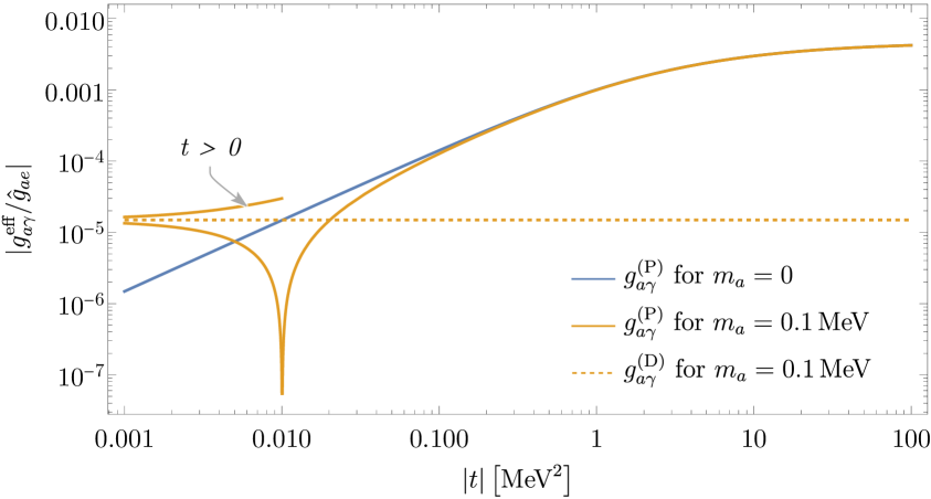
Figure 3: Effective ALP-photon couplings for $m_{\gamma}=0$: $g_{a\gamma}^{\text{(P)}}$ evaluated as function of the Mandelstam variable $t$ for $m_{a}=0$ (solid blue) and $m_{a}=0.1\,\text{MeV}$ (solid orange); and $g_{a\gamma}^{\text{(D)}}$ for $m_{a}=0.1\,\text{MeV}$ (dashed orange). Note that $g_{a\gamma}^{\text{(D)}}=0$ for $m_{a}=0$, and that $t$ is negative unless marked differently.

For high-energy photons with $\omega\gg m_{e}$, the effective Primakoff coupling of figure 3 approaches a constant value:

$$g_{a\gamma}^{\text{(P)}}\xrightarrow{\omega/m_{e}\to\infty}\frac{2\alpha}{\pi}\hat{g}_{ae}\,,$$ (2.9)

This limit is relevant e.g. when $m_{a}$ or $m_{\gamma}\gg m_{e}$, or when the process occurs in a highly relativistic QED plasma. Interestingly, $g_{a\gamma}^{\text{(P)}}$ in the limit of equation 2.9 agrees with $g_{a\gamma}^{\text{(D)}}$ in the $m_{e}\to 0$ limit. This is a consequence of the well-known anomaly: if the ALP couples to an (effectively) massless fermion, a chiral redefinition of the fermion field can eliminate the ALP-fermion coupling. However, since the PQ current is anomalous, the path integral measure is not invariant under this rotation and an ALP-photon coupling with precisely the value in equation 2.9 is generated. Hence, in the $m_{e}\to 0$ limit, the Lagrangian in equation 2.1 is equivalent to one where the ALP only couples to photons, and not the electron. Therefore, in this limit it is natural that the effective decay coupling matches with the effective Primakoff coupling.

Equation 2.9 also has interesting implications for more general ALP theories that include multiple charged fermions with different masses. In such theories, it is possible to assign PQ-charges to cancel the electromagnetic anomaly, in which case the total $g_{a\gamma}^{\text{(P)}}$ goes to zero in the large $t$ limit. However, even in this case, $g_{a\gamma}^{\text{(P)}}$ does not vanish at intermediate energies because the various contributions are sensitive to the ratio of $t$ to the fermion masses.

Due to the $t$-dependence of $g_{a\gamma}^{\text{(P)}}$, it is non-trivial to reinterpret current bounds on $g_{a\gamma}$ as bounds on $\hat{g}_{ae}$ through the loop process: most of those constraints involve integrals over a distribution of ALP-energies and the angle $\theta$, and therefore cannot just be “translated” by rescaling into limits on $\hat{g}_{ae}$. Instead, the resulting processes must be re-evaluated with the $t$-dependent effective coupling. In sections 3 to 5, we exemplify how this can be done when calculating ALP bounds from supernovae.

We close this section by briefly commenting on how our results relate to the previous literature on this subject. The loop induced coupling has been considered in [15], where SN bounds on $g_{a\gamma}$ were directly translated to $\hat{g}_{ae}$ using the decay coupling. As we have explained, this yields the wrong results for the Primakoff process: for ALP masses below $\sim 30$ MeV, using the decay coupling underestimates the bound by roughly a factor $\frac{m_{a}^{2}}{12m_{e}^{2}}$, which can be as small as $\sim 10^{-5}$ in the mass range considered in [15]. Moreover, reference [40] considered muons coupled to ALPs with either a derivative interaction proportional to $\hat{g}_{a\mu}$ analogous to this work, or a pseudoscalar coupling $g_{a\mu}$ as discussed below equation 2.1. For the latter, pseudoscalar case the resulting decay coupling $g_{a\gamma}^{\text{(D)}}$ was used to evaluate the one-loop Primakoff effect, and to derive constraints on $g_{a\mu}$ from the energy loss of SNe and horizontal branch stars. While this is strictly not correct, it turns out that for a pseudoscalar muon interaction the decay coupling approximates the actual Primakoff coupling quite well, for the relevant energies and masses, and corrections are small. For the case of derivatively coupled ALPs, as they are studied here, $g_{a\gamma}^{\text{(P)}}$ is not necessarily negligible, which was assumed in [40], and the inclusion of the muon-loop induced Primakoff effect would be an interesting extension of this work (see also section 7.2)

We have shown that $g_{a\gamma}^{\text{eff}}$ depends not only on the mass of the ALP, but more generally on the square of the four-momenta of ALP and photons. The effective coupling of the Primakoff process can be large if the energy of the ingoing photon is large compared to the electron mass. Thus, one should expect this one-loop effect to be particularly important in plasmas with temperatures $T\gtrsim 1$ MeV. An astrophysical system with such temperatures are core-collapse supernovae, and we now show how to derive new bounds from SN1987A using the loop-induced coupling.

3 Production of ALPs in SN1987A

Core-collapse supernovae offer an excellent opportunity to probe physics beyond the standard model because of the high temperatures and densities that are reached during the collapse. This enables exotic particles to be produced in potentially large numbers. ALPs can be produced in SNe through their couplings to any number of standard model particles like photons, electrons, nucleons, pions, or muons [16, 17, 41, 42, 43, 18, 44, 45, 46, 40].

In this section, we first describe the state-of-the-art supernova model of [19] in section 3.1, and provide an overview of the ALP production mechanisms in section 3.2. We then describe the detailed calculations for production through Bremsstrahlung in section 3.2.1, electron-positron fusion in section 3.2.2, Primakoff production in section 3.2.3 and photon coalescence in section 3.2.4. The first two processes occur at tree-level, while the latter two respectively depend on the one-loop coupling $g_{a\gamma}^{\text{(P)}}$ and $g_{a\gamma}^{\text{(D)}}$. Our discussion on how to use the resulting spectra to constrain ALPs is deferred to sections 4 and 5.

3.1 Supernova model

The production rate of ALPs in a SN plasma depends on a number of quantities, such as the temperature $T$, the mass density $\rho$, the electron chemical potential $\mu_{e}$, the effective number of protons $n_{p}^{\text{eff}}$ (a measure of number density as well as degeneracy), and the plasma frequency $\omega_{\text{pl}}$. All these quantities vary with position and time as the SN explosion is an inhomogeneous and dynamical process. As a numerical model for those profiles, we use the reference run of the SN simulations in [19], which uses the AGILE-BOLTZTRAN code [47, 48], assumes an 18 solar masses progenitor star, and spherical symmetry (i.e. the simulations are one dimensional). The model involves six-species Boltzman neutrino transport and includes contributions from muons and their weak interactions. As in [19], we use the relativistic mean-field nuclear equation of state DD2 as first described in [49] to infer the protons’ thermodynamical properties, e.g. $n_{p}^{\text{eff}}$.

We note that the specific properties of the SN models are not tightly constrained by observations, and hence the ALP production rates can vary by a factor of up to an order of magnitude depending on the model employed, see e.g. discussions in [43, 42]. The ALP production rates scale as $\sim\hat{g}_{ae}^{2}$, and hence, the final limits on the ALP-electron coupling will have a square-root sensitivity to the uncertainties in the astrophysical production spectra.

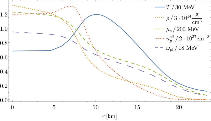
Figure 4: Some of the SN properties at $t=1$ s, taken from the simulations of [19]. At small radii, the finite resolution of the data is clearly visible.

Figure 4 shows some normalised profiles at $t=1$ second after the “bounce”, i.e. the time at which the central density in the SN core reaches its highest value. While the matter density and electron chemical potential fall monotonically, the temperature has a maximum at $r\simeq 10$ km. Therefore, we will find that all ALP production processes are most efficient near this radius (at $t=1$ s).

In general, there will be a back-reaction of the additional cooling and energy transfer by the ALPs on the SN evolution, so that a more accurate treatment would include the ALPs and their interactions in the described SN simulations, see [50, 19, 51]. Such an analysis is, however, beyond the scope of this work, which is why we take the data of the reference run of [19], i.e. the simulations without any ALPs, as an SN model, and treat the ALPs as small perturbation that will not affect the relevant dynamics.

With the numerical model at hand, we can now proceed to determine the flux and energy of the ALPs produced by this supernova model.

3.2 ALP production processes

(a) Bremsstrahlung

(b) Electron-positron fusion

(c) Primakoff process

(d) Photon coalescence

Figure 5: Relevant ALP production processes in SN1987A. The shaded blob in the lower two diagrams represents the one-loop, effective ALP photon interaction defined in equation 2.2.

In the following, we calculate the ALP production spectra $\frac{\mathrm{d}^{2}n}{\mathrm{d}t\,\mathrm{d}\omega}$, i.e. the number density of ALPs produced per time and energy, of the four relevant processes in SN1987A, shown in figure 5: the tree-level processes electron-nucleon Bremsstrahlung and electron-positron fusion, and one-loop processes of Primakoff production and photon coalescence. The spectra can be calculated as collision terms in the Boltzmann equation. We assume that all particles but the ALP are in thermal equilibrium, that this thermal bath is not influenced by the ALP production, and that the ALP phase space density is negligible so that no stimulated emission factor has to be included. This yields the following expression (see e.g. [52]):

$$\begin{split}\frac{\mathrm{d}^{2}n}{\mathrm{d}t\,\mathrm{d}\omega}=\Bigg{[}&\prod_{i}\int\frac{\mathrm{d}^{3}{\bf p}_{i}}{(2\pi)^{3}2E_{i}}f_{i}(E_{i})\Bigg{]}\Bigg{[}\prod_{j\neq a}\int\frac{\mathrm{d}^{3}{\bf p}^{\prime}_{j}}{(2\pi)^{3}2E^{\prime}_{j}}\left[1\pm f_{j}(E^{\prime}_{j})\right]\Bigg{]}\\ &\times(2\pi)^{4}\delta^{(4)}\Bigg{(}\sum_{i}p_{i}-\sum_{j}p^{\prime}_{j}\Bigg{)}S\,\,\frac{\lvert{\bf p}^{\prime}_{a}\rvert}{4\pi^{2}}\lvert\mathcal{M}\rvert^{2}\,,\end{split}$$ (3.1)

where ${\bf p}_{i},\,E_{i}$ are the incoming particles’ momenta and energies, ${\bf p}^{\prime}_{j},\,E^{\prime}_{j}$ those of the outgoing particles including the ALP, $f_{i,j}$ are the respective phase-space distribution functions, $|\mathcal{M}|^{2}$ is the squared matrix element summed over initial and final state polarisations, and $S=1/n!$ is a symmetry factor to avoid overcounting of $n$ identical particles in the initial or the final state. The quantum statistical factor for a final state particle is $1+f_{j}$ if $j$ represents a boson, and $1-f_{j}$ for a fermion. Note that the product over final state momenta does not include the ALP’s phase space as $\frac{\mathrm{d}^{2}n}{\mathrm{d}t\,\mathrm{d}\omega}$ is a differential with respect to the ALP’s energy in the plasma frame; the difference between the differentials of energy and Lorentz-invariant phase space yields the factor $\frac{\lvert{\bf p}^{\prime}_{a}\rvert}{4\pi^{2}}$.

From the production spectra, the ALP emissivity $Q$, i.e. the energy-loss rate per unit volume, can be determined as

$$Q=\int_{m_{a}}^{\infty}\mathrm{d}\omega\,\omega\frac{\mathrm{d}^{2}n}{\mathrm{d}t\,\mathrm{d}\omega}\,,$$ (3.2)

with the ALP energy $\omega$. Note that $Q$ in this form does not take reabsorption effects into account, see section 4.1 for the inclusion of those.

We will use the following definitions of the Bose-Einstein and Fermi-Dirac distributions, describing the phase space densities of photons, electrons and positrons, respectively:

$$f_{\text{\scriptsize B}}(\omega)=\frac{1}{\exp(\omega/T)-1}\,,\qquad f_{\text{\scriptsize F}}^{\mp}(E)=\frac{1}{\exp[(E\mp\mu_{e})/T]+1}\,,$$

with temperature $T$ and electron chemical potential $\mu_{e}$. We assume that electrons and positrons are in chemical equilibrium and therefore the positrons have chemical potential $-\mu_{e}$.

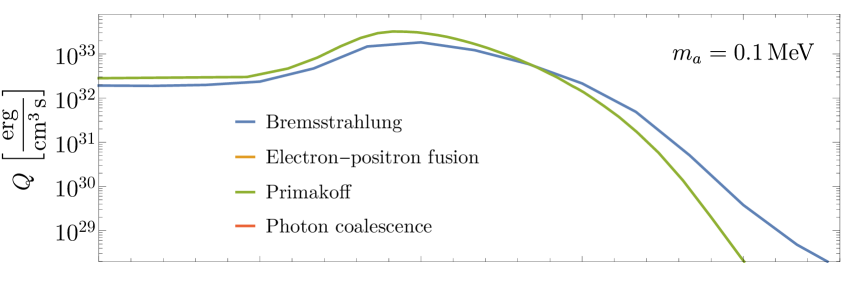
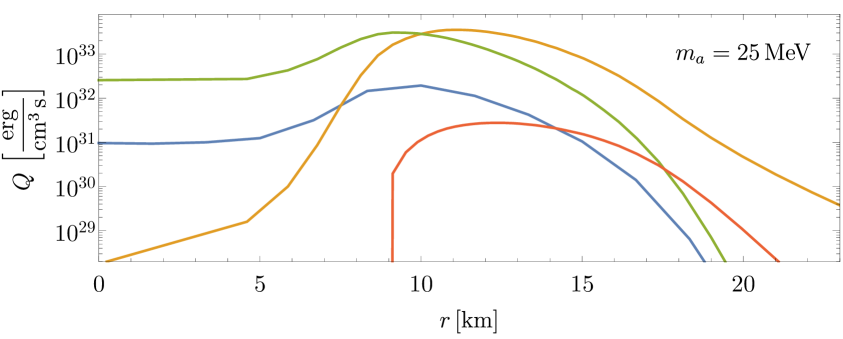
Figure 6: Comparison of ALP emissivity contributions of the four described processes for a low and a high mass, with $\hat{g}_{ae}=10^{-9}\text{ MeV}^{-1}$ in both plots. In the upper plot, $m_{a}$ is below the threshold for both inverse decays and thus the emissivity of those processes is zero. The same happens in the lower plot for photon coalescence at $r\leq 9$ km.

Figure 6 anticipates the results of sections 3.2.1 to 3.2.4, and shows the emissivities of the four ALP production processes for different masses. One of the main, unexpected results of this paper is that the loop-induced Primakoff process results in the largest ALP emissivity and fluence at small radii (see section 3.2.3). Other qualitative properties of the production spectra depend on the mass of the ALP. At low masses ($m_{a}\lesssim 20$ MeV), the Bremsstrahlung and Primakoff contributions dominate at all radii as inverse decays (i.e. electron-positron fusion and photon coalescence) are suppressed, or even kinematically forbidden. At higher masses and for sufficiently large radii, the tree-level electron-positron fusion process quickly dominates as it becomes kinematically available.

We now discuss, in turn, how the production spectra for Bremsstrahlung, electron-positron fusion, the Primakoff process, and photon coalescence are calculated.

3.2.1 Bremsstrahlung

Electron-ion Bremsstrahlung, shown in figure 5(a), is the leading production process at tree-level for ALPs with masses $m_{a}\lesssim 30~{}\text{MeV}$ in hot, degenerate plasmas [1, 18]. As the upper panel of figure 6 shows, in our model the contribution of the tree-level Bremsstrahlung process to the ALP emissivity is dominant at large radii, i.e. at low temperatures, but remains non-negligible at all radii.

Equation 3.1 yields the following expression for the production spectrum of ALPs created by electron-ion Bremsstrahlung:

$$\frac{\mathrm{d}^{2}n}{\mathrm{d}t\,\mathrm{d}\omega}=\frac{n_{p}^{\text{eff}}}{64\pi^{6}}\int_{-1}^{1}\mathrm{d}c_{1a}\,\int_{-1}^{1}\mathrm{d}c_{12}\,\int_{0}^{2\pi}\mathrm{d}\delta\,\int_{m_{e}}^{\infty}\mathrm{d}E_{2}\left\lvert\mathbf{p}_{1}\right\rvert\left\lvert\mathbf{p}_{2}\right\rvert\left\lvert\mathbf{p}_{a}\right\rvert\left\lvert\mathcal{M}\right\rvert^{2}f_{\text{\scriptsize F}}^{-}(E_{1})\left(1-f_{\text{\scriptsize F}}^{-}(E_{2})\right)\,,$$ (3.3)

where $E_{1,2}$ are the incoming and outgoing electrons’ energies, respectively, while the outgoing ALP has energy $\omega$, the ${\bf p}_{i}$ are the respective momenta, $c_{1a}\,(c_{12})$ is the cosine of the angle between the incoming electron and ALP (outgoing electron) momenta, and $\delta$ the angle between the two planes spanned by these momentum pairs. This expression agrees with [18]. Since the ion has masses in the GeV-range, and hence does essentially not recoil when scattering with thermal electrons in a plasma with $T\lesssim 40$ MeV, energy conservation implies $E_{1}=\omega+E_{2}$.

Furthermore, we consider only free protons as target-ions, since electrons are highly degenerate in the SN core, and ALP production is most efficient at high temperature where no nuclear clustering occurs [42]. Therefore, the number density of targets is the effective number density of protons, taking their degeneracy into account [41]

$$n_{p}^{\text{eff}}=2\int\frac{\mathrm{d}^{3}p}{(2\pi)^{3}}f_{p}(1-f_{p})\,,$$ (3.4)

which can be up to $60\%$ smaller than the naive number density, without the factor $(1-f_{p})$, of free protons in SN1987A [42]. The effective density $n_{p}^{\text{eff}}$ factors out of the expression for the spectrum in equation 3.3 because we assume no proton recoil.

The matrix element for this process, $\left\lvert\mathcal{M}\right\rvert^{2}$, averaged over the incoming and outgoing electrons’ spin, can be found in the appendix of [53], where the authors use $k_{S}^{2}T=e^{2}n_{p}^{\text{eff}}$ and include $n_{p}^{\text{eff}}$ in the definition of $\lvert\mathcal{M}\rvert^{2}$, which we do not. We used FeynCalc to reproduce and check the expression, and find agreement with [53]. It should be noted that references [53] and [18] used the pseudoscalar interaction between ALPs and electrons and that results are stated in terms of the dimensionless coupling $g_{ae}$. We checked that using the derivative coupling as included in equation 2.1 leads to the same matrix element after the replacement $\hat{g}_{ae}\to g_{ae}/(2m_{e})$.

The propagation of electrons and positrons in a relativistic QED plasma is significantly different from vacuum propagation. In [18] the authors argue that for ALP production in SN1987A, it is sufficient to replace the vacuum electron mass $m_{e}\simeq 511\text{ keV}$ by an effective mass depending on temperature and chemical potential:

$$m_{e}^{\text{eff}}=\frac{m_{e}}{\sqrt{2}}+\sqrt{\frac{m_{e}^{2}}{2}+\frac{\alpha}{\pi}\left(\mu_{e}^{2}+\pi^{2}T^{2}\right)}\,,$$ (3.5)

which corresponds to $\sqrt{2}m_{e}^{\star}$ in the notation of [18]. Note that this form of the effective mass is only valid for $m_{e}^{\text{eff}}\gg m_{e}$, i.e. large $T$ or $\mu$ [54], explaining why the $T,\mu\to 0$ limit yields $m_{e}^{\text{eff}}\to\sqrt{2}m_{e}>m_{e}$. We will use this effective mass whenever we calculate the ALP-electron tree-level processes in the SN core (i.e. Bremsstrahlung, electron-positron fusion and their respective inverses).

However, in [18] it was argued that the equivalence between pseudoscalar and derivative ALP-electron couplings also holds unaltered in the plasma, but remarkably, the two different couplings only lead to the same results if the replacement $\hat{g}_{ae}\to g_{ae}/(2m_{e})$ is done with the vacuum electron mass $m_{e}$. We note that, therefore, by using the derivative coupling and naively following the prescription of [18], i.e. replacing $m_{e}\to m_{e}^{\text{eff}}$ everywhere, one would actually underestimate the Bremsstrahlung and electron-positron fusion rates by typically more than two orders of magnitude. We leave a further investigation of this puzzle to future work.

The contribution of the Bremsstrahlung process to the ALP emissivity in SN1987A is shown in blue in figure 6.

3.2.2 Electron-positron fusion

If the ALP mass is larger than twice the effective electron mass, there is a further, and usually more efficient production process at tree-level: the inverse of the ALP-to-electron decay, electron-positron fusion. The diagram is shown in figure 5(b), yielding the matrix element, averaged over initial states, $\frac{1}{4}\lvert\mathcal{M}\rvert^{2}=g_{ae}^{2}m_{a}^{2}/2$. The resulting production spectrum can be calculated by integrating the electron and positron distribution functions over the positron energy $E_{+}$

$$\frac{\mathrm{d}^{2}n}{\mathrm{d}t\,\mathrm{d}\omega}=\frac{g_{ae}^{2}m_{a}^{2}}{16\pi^{3}}\,\Theta(m_{a}-2m_{e}^{\text{eff}})\int_{E_{\text{min}}}^{E_{\text{max}}}\mathrm{d}E_{+}\,f_{\text{\scriptsize F}}^{-}(\omega-E_{+})f_{\text{\scriptsize F}}^{+}(E_{+})\,,$$ (3.6)

with the ALP energy $\omega$, energy conservation yielding $\omega-E_{+}$ as the electron energy, and momentum conservation leading to the lower and upper integration limits

$$E_{\text{min,max}}=\frac{\omega}{2}\mp\frac{\sqrt{(\omega^{2}-m_{a}^{2})(m_{a}^{2}-4(m_{e}^{\text{eff}})^{2})}}{2m_{a}}\,.$$ (3.7)

This expression again agrees with [18]. Note that, as in [18], we use the pseudoscalar coupling $g_{ae}$ in equation 3.6 following our earlier arguments (see section 3.2.1) about the thermal modification of the ALP electron interaction in a plasma. As also discussed there, we have to use the effective, thermal electron mass $m_{e}^{\text{eff}}$ defined in equation 3.5 to take the effect of the plasma on electron and positron propagation into account.

We remark here that the integrand in equation 3.6 peaks for small $E_{+}$ because the positrons have chemical potential $-\mu_{e}$ with $\mu_{e}\gg T$ and hence their distribution function is approximately $f_{\text{\scriptsize F}}^{+}(E_{+})\sim\exp(-E_{+}/T)$. Therefore, in this particular case it is not clear that the modification of the positrons’ dispersion relation is captured well by the simple replacement $m_{e}\to m_{e}^{\text{eff}}$, as this approximation is valid only for hard momenta $p_{+}=\sqrt{E_{+}^{2}-\left(m_{e}^{\text{eff}}\right)^{2}}\gg m_{e}^{\text{eff}}$ [54]. In the scope of this work, we follow the literature in using the effective mass approximation for electron-positron fusion, and leave the question of how accurate the approximation is for further study.

The contribution of electron-positron fusion to the ALP emissivity in SN1987A is shown in orange in figure 6. In the upper plot the ALP mass is too low for electron-positron fusion to be allowed kinematically, so the production spectrum is zero.

3.2.3 Primakoff process

One of the main phenomenological result of this paper is the accurate determination of the contribution of the loop-induced Primakoff process to ALP production in hot, dense plasmas. We find that it is in fact the leading production process for $m_{a}\lesssim 20$ MeV.

In the Primakoff process, a photon converts into an ALP in the field of a charged fermion, shown in the diagram in figure 5(c). As for Bremsstrahlung, the main target fermion is a free proton, since electrons are degenerate and almost no nuclei can form in the SN core.

With our definition of the effective Primakoff ALP-photon coupling in equation 2.8 the differential cross-section of the process can be written compactly as [55]

$$\frac{\mathrm{d}\sigma_{\text{P}}}{\mathrm{d}\Omega}=\left\lvert g_{a\gamma}^{\text{(P)}}(\omega,\cos\theta)\right\rvert^{2}\frac{\alpha}{8\pi}\frac{p_{\gamma}p_{a}^{3}(1-\cos^{2}\theta)}{(p_{\gamma}^{2}+p_{a}^{2}-2p_{\gamma}p_{a}\cos\theta)(p_{\gamma}^{2}+p_{a}^{2}-2p_{\gamma}p_{a}\cos\theta+\kappa_{\text{S}}^{2})}\,,$$ (3.8)

where we have used the limit of no ion recoil again, i.e. $m_{\text{ion}}\to\infty$, in which case energy conservation implies that both photon and ALP have energy $\omega=\sqrt{p_{a}^{2}+m_{a}^{2}}=\sqrt{p_{\gamma}^{2}+m_{\gamma}^{2}}$, with the respective momenta $p_{a,\gamma}$, and $\theta$ is the angle between the momentum vectors. For processes with external photons, it is important to note that in the SN plasma on-shell photons acquire an effective mass [56]:

$$m_{\gamma}=\omega_{\text{pl}}\simeq 16.3\operatorname{MeV}Y_{e}^{1/3}\left(\frac{\rho}{10^{14}\operatorname{g}\operatorname{cm}^{-3}}\right)^{1/3}\,,$$ (3.9)

where $\omega_{\text{pl}}$ is the plasma frequency and $Y_{e}$ the electron fraction. Furthermore, equation 3.8 includes the screening of the Coulomb-like interaction at the Debye-Hückel scale $\kappa_{\text{S}}^{2}=e^{2}n_{p}^{\text{eff}}/T$ [55].

The resulting ALP spectrum is

$$\frac{\mathrm{d}^{2}n}{\mathrm{d}t\,\mathrm{d}\omega}=\frac{n_{p}^{\text{eff}}}{\pi^{2}}\frac{\omega^{2}-m_{\gamma}^{2}}{\exp(\omega/T)-1}\sigma_{\text{P}}\,,$$ (3.10)

where $\sigma_{\text{P}}$ is the total cross section, and the density of target protons factors out because of the no-recoil limit as in the case of Bremsstrahlung. Note that we cannot analytically solve the integral over $\cos\theta$ in the definition of the total cross section since the effective coupling has a non-trivial dependence on $\cos\theta$. Therefore, we have to evaluate the implicit integral in equation 3.10 numerically.

For energies $\omega\gg m_{a},m_{\gamma},m_{e}$ we can approximate $g_{a\gamma}^{\text{(P)}}\simeq\frac{2\alpha}{\pi}\hat{g}_{ae}$, and in that case give a simple expression for the emissivity

$$Q\simeq\frac{\alpha^{2}\hat{g}_{ae}^{2}}{\pi^{3}}\,T^{7}F\left(\frac{\kappa_{\text{S}}^{2}}{4T^{2}}\right)\,,$$ (3.11)

where $F$ is defined in [55], slowly varying, and of order $10^{-2}$ to $10^{-1}$ for typical SN conditions. We see that the Primakoff emissivity depends strongly on the temperature, explaining why it can be the leading production process in the hot SN plasma, even though it is suppressed by a loop factor. In figure 6 the Primakoff contribution is shown in green.

In the literature, one often finds a production rate $\Gamma_{\text{P}}$, see e.g. [1, 42], which is related to the production spectrum and the total cross section as

$$\Gamma_{\text{P}}=\pi^{2}\frac{\exp(\omega/T)-1}{\beta_{\gamma}\omega^{2}}\,\frac{\mathrm{d}^{2}n}{\mathrm{d}t\,\mathrm{d}\omega}=n_{p}^{\text{eff}}\beta_{\gamma}\sigma_{\text{P}}\,,$$ (3.12)

with $\beta_{\gamma}$ as defined in section 2.3. Replacing $g_{a\gamma}^{\text{(P)}}(\omega,\cos\theta)\to g_{a\gamma}$ in equation 3.12, and integrating the cross section yields the same expression for $\Gamma_{\text{P}}$ as in [42].

3.2.4 Photon coalescence

In close analogy to the electron-positron fusion process, there is also an inverse to ALP-to-photon decay called photon coalescence with the diagram shown in figure 5(d). Since in a plasma we have to treat the photons as massive with mass $m_{\gamma}$, the kinematics of the process are equivalent to the electron-positron fusion case with the replacement $m_{e}\to m_{\gamma}$. However, the averaged matrix element is slightly different $\frac{1}{4}\lvert\mathcal{M}\rvert^{2}=\frac{1}{8}\left\lvert g_{a\gamma}^{\text{(D)}}\right\rvert^{2}m_{a}^{4}(1-4m_{\gamma}^{2}/m_{a}^{2})$, and we find the following expression for the production rate:

$$\frac{\mathrm{d}^{2}n}{\mathrm{d}t\,\mathrm{d}\omega} =\left\lvert g_{a\gamma}^{\text{(D)}}\right\rvert^{2}\frac{m_{a}^{4}}{128\pi^{3}}\left(1-\frac{4m_{\gamma}^{2}}{m_{a}^{2}}\right)\,\Theta(m_{a}-2m_{\gamma})\int_{\omega_{\text{min}}}^{\omega_{\text{max}}}\mathrm{d}\omega_{1}\,f_{\text{\scriptsize B}}(\omega_{1})f_{\text{\scriptsize B}}(\omega-\omega_{1})$$ (3.13)

$$\xrightarrow{\omega\gg T}\left\lvert g_{a\gamma}^{\text{(D)}}\right\rvert^{2}\frac{m_{a}^{4}}{128\pi^{3}}\sqrt{\omega^{2}-m_{a}^{2}}\left(1-\frac{4m_{\gamma}^{2}}{m_{a}^{2}}\right)^{3/2}\exp\left(-\frac{\omega}{T}\right)\Theta(m_{a}-2m_{\gamma})\,.$$

The integration limits $\omega_{\text{min,max}}$ are given by equation 3.7 with $m_{e}\to m_{\gamma}$, and we show that in the limit $\omega\gg T$, i.e. if $f_{\text{\scriptsize B}}$ is well approximated by a Boltzmann distribution, the result of [42] is recovered. In the $m_{\gamma}\to 0$ limit this result also agrees with the expression found in the supplemental material of [57], which to our knowledge is the first time quantum statistics have been taken into account in the photon coalescence production rate. Therefore, equation 3.13 generalises both previous results by including an effective photon mass as well as the quantum distribution function for the photons.

The ALP emissivity due to photon coalescence is shown in red in figure 6. As is the case for electron-positron fusion, this inverse decay is kinematically only allowed when the ALP mass is large enough. In fact, in our SN model the effective photon mass is always larger than the effective electron mass (cf. equations 3.5 and 3.9), and hence, to be efficient, photon coalescence requires even larger $m_{a}$ than electron-positron fusion. This can be seen in the lower plot in figure 6 with $m_{a}=25$ MeV: the ALP emissivity due to photon coalescence goes to zero for radii below 9 km because there $m_{\gamma}(r)>m_{a}/2$, while electron-positron fusion is possible for all radii.

The production spectra calculated in this section will now be used to constrain the ALP-electron coupling via the so-called cooling bound in section 4, and the decay bound in section 5.

4 Cooling bound

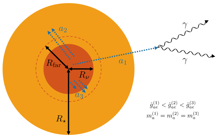
Figure 7: Mechanisms of the two supernova constraints for three different, exemplary ALP models $a_{i}$ with couplings $\hat{g}_{ae}^{(i)}$ and masses $m_{a}^{(i)}$. ALPs are predominantly produced in the neutrino sphere with radius $R_{\nu}$ (shown in dark orange), with the number of arrows indicating the respective flux; note that production in the actual model is isotropic and spherically symmetric. The ALPs will subsequently be reabsorbed by the SN plasma ($a_{2}$ and $a_{3}$) or decay into photons or electron-positron pairs where kinematically allowed (possible for all three depicted scenarios). The typical time and length scales after which reabsorption and decay happen depend on the coupling strength and, as depicted here, weaker couplings lead to longer mean-free paths. ALP $a_{1}$ will contribute both to the decay and cooling bound, $a_{2}$ only to the cooling bound since it does not escape the SN remnant with radius $R_{\star}$ (shown in orange), and $a_{3}$ to neither since it is absorbed before the radius $R_{\text{far}}$ as defined below. See full text for details.

An illustration of the SN constraints we consider here and in section 5 is shown in figure 7. In this section, we first examine how the SN plasma loses energy by ejecting ALPs, and why too much of this cooling is incompatible with observations.

The relevant observation here is that SN1987A was accompanied by a 10s long neutrino burst. As suggested by Raffelt in [1], a simple analytical estimate shows that the duration of this burst would roughly be cut in half if there was an additional energy loss channel at $t=1\,$s after the initial bounce with a luminosity as large as the one of neutrinos $L_{\nu}\simeq 3\cdot 10^{52}\frac{\operatorname{erg}}{\text{s}}$. Note that $L_{\nu}$ is taken from the SN simulations that we use [19]. As should be clear from the discussion in section 3, weakly coupled ALPs provide such an additional energy loss mechanism if they can escape the SN. Therefore, we can derive a constraint on their interactions with the plasma, which we assume to be just due to $\hat{g}_{ae}$, by demanding that

$$L_{a}<L_{\nu}\simeq 3\cdot 10^{52}\frac{\operatorname{erg}}{\text{s}}\,.$$ (4.1)

Before deriving the ALP luminosity in section 4.2, we first consider in section 4.1 that they can also be reabsorbed by the plasma.

4.1 ALP reabsorption and opacity

Due to the high temperature and large density in the supernova core, ALPs can be produced but also quickly absorbed if the coupling to electrons or photons is large enough. If this happens in the core of the SN, they do not contribute to the energy loss that is relevant for the shortening of the neutrino burst.

The relevant quantity characterising the ALP absorption is the local mean free path, defined as product of the (relativistic) velocity of the ALP $\beta_{a}=\sqrt{1-\left(\frac{m_{a}}{\omega}\right)^{2}}$ and the inverse of its reduced absorption rate $\Gamma_{\text{abs}}$ [40]:

$$\lambda=\beta_{a}\,\Gamma_{\text{abs}}^{-1}\,.$$ (4.2)

The reduced absorption rate is the difference between the absorption and spontaneous emission rates of the ALP, which due to detailed balance (see also equation 4.3) is equal to $1-\exp(-\omega/T)$ times the absorption rate [40].

To calculate the total reduced absorption rate, we include the inverses of all production processes mentioned above: Primakoff, Bremsstrahlung, Photon coalescence, and electron-positron fusion, where the latter two are just decays. The rates of the respective inverse processes can be calculated from the collision term, similar to equation 3.1, and are therefore related to the production spectra of section 3.2 as

$$\Gamma_{\text{abs}}=\frac{2\pi^{2}[\exp(\omega/T)-1]}{\beta_{a}\omega^{2}}\frac{\mathrm{d}^{2}n}{\mathrm{d}t\,\mathrm{d}\omega}\,,$$ (4.3)

where we used the following relations to convert initial and final state distribution factors into another:

$$1-f_{\text{\scriptsize F}}^{\mp}(E)=\exp\left(\frac{E\mp\mu}{T}\right)f_{\text{\scriptsize F}}^{\mp}(E)\,,\qquad 1+f_{\text{\scriptsize B}}(E)=\exp\left(\frac{E}{T}\right)f_{\text{\scriptsize B}}(E)\,.$$

These hold because we assume all particles except for the ALP to be in thermal equilibrium. Note that the rate $\Gamma_{\text{abs}}$ does not depend on the ALPs’ phase-space distribution, and therefore does not receive corrections at large couplings where interactions are more efficient and would eventually bring the ALPs into equilibrium with the plasma.

In the following, we determine the mean free paths of the four relevant processes and comment on some improvements over the existing calculations in the literature – apart from the inclusion of one-loop corrections.

Using equations 4.2, 4.3 and 3.3, we find that inverse Bremsstrahlung has a mean free path of

$$\begin{split}\lambda_{\text{B}}^{-1}&=\frac{n_{p}^{\text{eff}}[\exp(\omega/T)-1]}{32\pi^{4}}\\ &\quad\times\int_{-1}^{1}\mathrm{d}c_{1a}\,\int_{-1}^{1}\mathrm{d}c_{12}\,\int_{0}^{2\pi}\mathrm{d}\delta\,\int_{m_{\text{e}}}^{\infty}\mathrm{d}E_{2}\frac{\left\lvert\mathbf{p}_{1}\right\rvert\left\lvert\mathbf{p}_{2}\right\rvert}{\left\lvert\mathbf{p}_{a}\right\rvert}\left\lvert\mathcal{M}\right\rvert^{2}f_{\text{\scriptsize F}}^{-}(\omega+E_{2})\left[1-f_{\text{\scriptsize F}}^{-}(E_{2})\right]\,.\end{split}$$ (4.4)

Note that this expression differs by a factor $\frac{1-\exp(-\omega/T)}{\beta_{a}\pi}$ from the expression found in equation (31) of [18], where the numerator is due to the fact that the reduced absorption rate has not been used in [18].

For the ALP-to-electron decay, we find

$$\begin{split}\Gamma_{\text{abs}}^{a\to e^{+}e^{-}}&=\frac{g_{ae}^{2}m_{a}^{2}\left(e^{\omega/T}-1\right)}{8\pi\,\omega^{2}\beta_{a}}\,\Theta(m_{a}-2m_{e}^{\text{eff}})\int_{E_{\text{min}}}^{E_{\text{max}}}\mathrm{d}E_{+}\,f_{\text{\scriptsize F}}^{-}(\omega-E_{+})f_{\text{\scriptsize F}}^{+}(E_{+})\\ &=\frac{g_{ae}^{2}m_{a}^{2}\left(1-e^{-\omega/T}\right)}{8\pi\,\omega^{2}\beta_{a}}\,\Theta(m_{a}-2m_{e}^{\text{eff}})\int_{E_{\text{min}}}^{E_{\text{max}}}\mathrm{d}E_{+}\,\left[1-f_{\text{\scriptsize F}}^{-}(\omega-E_{+})\right]\left[1-f_{\text{\scriptsize F}}^{+}(E_{+})\right]\\ &\xrightarrow{T\to 0}\gamma_{a}^{-1}\,\Gamma_{0}^{a\to e^{+}e^{-}}\,,\end{split}$$ (4.5)

where $\Gamma_{0}^{a\to e^{+}e^{-}}$ is the usual ALP decay rate in its rest frame (see e.g. [38]), and $\gamma_{a}=\frac{\omega}{m_{a}}$ is the Lorentz factor. As explained in section 3.2.2, we take quantum statistics into account, which for the ALP-to-electron decay means a suppression of the rate by Pauli blocking due to the electrons present in the plasma. In the $T\to 0$ limit, i.e. when using Boltzmann statistics for the electrons (and not using the reduced absorption rate), we reproduce the rate used in [18]. However, ignoring Pauli blocking in a highly degenerate plasma overestimates the decay rate severely, by up to three orders of magnitude in the inner core of the SN.

In case of the inverse Primakoff effect, we find instead

$$\lambda_{\text{P}}^{-1}=2\,n_{p}^{\text{eff}}\left(\frac{\beta_{\gamma}}{\beta_{a}}\right)^{2}\,\sigma_{\text{P}}=2\,n_{p}^{\text{eff}}\left(\frac{\beta_{\gamma}}{\beta_{a}}\right)^{2}\sigma_{\text{P}}\,,$$ (4.6)

which is the same expression as in [42].

For the ALP-to-photon decay, equations 4.3 and 3.13 yield

$$\begin{split}\Gamma_{\text{abs}}^{a\to\gamma\gamma}&=\frac{\big{\lvert}g_{a\gamma}^{\text{(D)}}\big{\rvert}^{2}m_{a}^{2}(m_{a}^{2}-4m_{\gamma}^{2})}{64\pi\beta_{a}\,\omega^{2}}\left(e^{\omega/T}-1\right)\,\Theta(m_{a}-2m_{\gamma})\int_{\omega_{\text{min}}}^{\omega_{\text{max}}}\mathrm{d}\omega_{1}\,f_{\text{\scriptsize B}}(\omega_{1})f_{\text{\scriptsize B}}(\omega-\omega_{1})\\ &=\frac{\big{\lvert}g_{a\gamma}^{\text{(D)}}\big{\rvert}^{2}m_{a}^{2}(m_{a}^{2}-4m_{\gamma}^{2})}{64\pi\beta_{a}\,\omega^{2}}\left(1-e^{-\omega/T}\right)\Theta(m_{a}-2m_{\gamma})\\ &\qquad\times\int_{\omega_{\text{min}}}^{\omega_{\text{max}}}\mathrm{d}\omega_{1}\,\left[1+f_{\text{\scriptsize B}}(\omega_{1})\right]\left[1+f_{\text{\scriptsize B}}(\omega-\omega_{1})\right]\\ &\xrightarrow{T\to 0}\left\lvert g_{a\gamma}^{\text{(D)}}\right\rvert^{2}\frac{m_{a}^{4}}{64\pi\,\omega}\left(1-\frac{4m_{\gamma}^{2}}{m_{a}^{2}}\right)^{3/2}=\gamma_{a}^{-1}\,\Gamma_{0}^{a\to\gamma\gamma}\,,\end{split}$$ (4.7)

where also here $\Gamma_{0}^{a\to\gamma\gamma}$ is the decay rate in the ALP rest frame (see e.g. [38]). As in the case of the electron decay, quantum statistics influence the rate, which in this case is Bose enhanced. Here, the effect is smaller than in the case of decay into electron-positron pairs, but can still enlarge the rate by a factor of 2 for typical SN values. Ignoring bose enhancement (and the reduction of the absorption rate), we reproduce the rate given in [42].

4.2 Modified luminosity criterion

As mentioned in the beginning of this section, if the ALPs produced in SN1987A carry away enough energy from the region from which the observed neutrino burst originated – the so-called “neutrino sphere” with radius $R_{\nu}$ – the duration of this burst would shorten. Thus, the ALP has to couple either weakly enough so that no relevant abundance is produced in the SN, or so strongly that most of the emitted ALPs are reabsorbed by the plasma before they leave the SN core.

To implement this bound, we follow the procedure of [58], which was adopted to ALPs in [59, 43, 42, 18]: we integrate the energy carried away by ALPs from the neutrino sphere with radius $R_{\nu}$, which are not reabsorbed before they reach the neutrino gain radius $R_{\text{far}}$ [42] (see figure 7 for an illustration of these radii). If an ALP’s energy is deposited back into the plasma before it reaches $R_{\text{far}}$, the energy could be converted into neutrinos since they are still produced efficiently in this region. Hence, the energy deposited into such an ALP does not shorten the neutrino burst and should not be included in equation 4.1. The modified luminosity $L_{a}$ is the relevant quantity in this inequality; it is the cooling power of ALPs that cannot be efficiently reconverted into neutrinos. The modified luminosity can be calculated as the following integral over the neutrino sphere and the ALP energy, including the absorption factor $\exp\left[-\tau(r,\omega)\right]$ where $\tau$ is the ALP’s “optical depth” [58]:

$$L_{a}=\int_{0}^{R_{\nu}}\mathrm{d}r\,4\pi r^{2}\,\ell^{2}(r)\int_{m_{a}/\ell(r)}^{\infty}\mathrm{d}\omega\,\omega\,\frac{\mathrm{d}^{2}n}{\mathrm{d}t\,\mathrm{d}\omega}(r,\omega)\cdot e^{-\tau(r,\omega)}\,,$$ (4.8)

where we fix $R_{\nu}=21$ km and $R_{\text{far}}=24$ km following [18]. The lapse function $\ell(r)\in[0,1]$ accounts for relativistic corrections in two ways: first, ALPs with local energy $\omega<m_{a}/\ell$ will be gravitationally trapped in the SN, and second, the energy observed at infinity is red-shifted compared to the local one, while the local time is dilated [57]. We take the approximated, general relativistic lapse function from the SN simulation [19]. The optical depth is an integral over the inverse local mean free path

$$\tau(r,\omega)=\int_{r}^{R_{\text{far}}}\frac{\mathrm{d}\tilde{r}}{\lambda_{\text{total}}(\tilde{r},\omega)}\,.$$ (4.9)

We improve on the treatment of absorption in [42] by integrating over the energy dependent optical depth in equation 4.8 instead of approximating $\tau(r,\omega)\simeq\tau(r,\langle\omega\rangle)$ in the integral, where $\langle\omega\rangle$ is the average ALP energy (cf. [43, 18]).

Figure 8: Bounds on the ALP-electron coupling from anomalous cooling with only tree-level ALP-electron interactions (dashed blue line), and including also the loop-induced ALP-photon interactions (red region), see section 4. Our bounds can be compared with the existing tree-level cooling bound from [18] (black line). Bounds from the decay into gamma-ray photons (orange region), see section 5.

We get the cooling bound on the ALP-electron coupling by demanding that the modified luminosity in ALPs should not be larger than the luminosity in neutrinos $L_{a}<L_{\nu}\simeq 3\times 10^{52}\text{erg}\text{ s}^{-1}$ [58]. The resulting exclusion region is shown in figure 8.

The upper boundary of this region lies in the so-called trapping regime: the ALPs are so strongly coupled that most of them are absorbed before they can escape the gain radius $R_{\text{far}}$, decreasing the modified luminosity exponentially with increasing coupling. For large masses $m_{a}\gtrsim 2$ MeV, the dominating absorption processes are decays, mostly into electron-positron pairs, which become more efficient the heavier the ALP is. Therefore, we see that the upper end of the exclusion region decreases at larger masses. At very large masses $m_{a}\gtrsim 250$ MeV, Boltzmann suppression of the ALP production cuts off the bound as the ALPs become to heavy to be produced in a plasma with $T\sim 30$ MeV.

Near the lower boundary of the exclusion region, the ALPs can free-stream out of the SN plasma without relevant absorption events. Here, the constraint is determined only by the production spectra of ALPs. As we have seen in section 3, the production is dominated by the Primakoff process for masses of $m_{a}\lesssim 20$ MeV, while for heavier ALPs the inverse decays are more efficient.

For comparison, we show the cooling bound that would result from only the tree-level ALP-electron interactions as dashed blue boundary in figure 8. For masses $m_{a}<20$ MeV there is an improvement of up to a factor of 2.4 in the free-streaming regime, i.e. at small couplings. In this part of parameter space, the Primakoff process contributes around as much to ALP production as Bremsstrahlung, see also figure 6. In the trapping regime, i.e. for large couplings, the loop-level processes seem not to contribute significantly to the modified luminosity.

We also include the bound of [18] in figure 8 in black for reference. This bound is the equivalent of the blue tree-level bound calculated here. The discrepancy at large masses is due to Pauli blocking, which as we discussed in section 4.1 strongly suppresses the decay of ALPs to electron-positron pairs, and which was not taken into account in [18]. At small masses, the inverse Bremsstrahlung absorption process was significantly overestimated in that reference. Finally, gravitational red-shift and trapping effects were not included in the analysis of [18], which leads to a slightly stronger bound for small couplings.

5 Decay bound

Apart from the indirect bound on ALPs as extra cooling channel of the SN core, one can also infer a bound directly from the non-observation of gamma-rays in the energy band $25-100$ MeV after the explosion. Since the ALPs produced in the SN core via the processes studied in section 3.2 typically have energies in this range, and can decay into photons after they leave the plasma, a certain number of gamma-ray photons should have been observed by the gamma-ray spectrometer (GRS) on board of the Solar Maximum Mission (SMM) satellite. Even though the GRS was directed towards the sun when the neutrino burst of SN1987A was observed on earth, gamma-rays from the direction of SN1987A would have hit the satellite on the side, would have penetrated the shielding, and thus still reached the detector [61]. The GRS was taking data for 223 seconds after arrival of the initial neutrino burst, but went into calibration mode afterwards. One can put a bound on the number of ALPs produced in the SN since no excess gamma-rays were observed during this time [61]. This bound has been considered before, most recently in [62] where a tree-level coupling of ALPs and photons was assumed, and in [40] where couplings to muons were considered at tree-level.

As opposed to the cooling bound, there is no tree-level analog here for ALPs only coupled to electrons: while they can be produced in significant amounts as we have seen, at tree-level they can only decay into electrons and positrons after leaving the SN plasma. Although charged particles are not expected to reach earth, their interaction with e.g. CMB photons or the extragalactic background light, could potentially still lead to the production of photons with $25-100$ MeV energies. These secondary processes would require a dedicated analysis. Here we will only consider the photons that result from the the decay of the ALP outside the SN via the loop process.

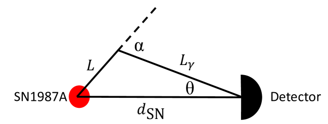
Figure 9: Geometry of the ALP decay into a gamma-ray photon reaching earth. The ALP travels a distance $L$ before it decays into a photon under an angle $\alpha$. The photon travels a distance $L_{\gamma}$ before it reaches the detector under an angle $\theta$. The number of ALPs reaching the detector on the side opposite to the SN is negligible (see text) so that $\cos\theta>0$, while the angles are only part of a triangle as shown if $\cos\theta>\cos\alpha$.

The quantity we can ultimately compare to observations is $F_{\gamma}$, the fluence of gamma-ray photons with energies between 25 and 100 MeV arriving at SMM in a time-window of $\Delta t_{\text{max}}=223s$ after the initial neutrino burst was detected. The source of $F_{\gamma}$ is the ALP fluence outside of the supernova plasma. However, considering only the fluence of the source is not a good estimate for $F_{\gamma}$, not even for its order of magnitude. We have to take into account several factors yielding the probability of a given ALP to decay into a photon and for this photon to be observed by the detector. This probability distribution depends on three variables: the energy of the ALP $\omega$, the cosine of the angle under which the ALP decays into photons $c_{\alpha}\equiv\cos\alpha$, and the distance the ALP travels before it decays $L$. Following a very similar discussion for neutrinos in [63], we can write the differential fluence of gamma-ray photons as

$$\mathrm{d}F_{\gamma}=2\cdot\mathrm{BR}_{a\to\gamma\gamma}\cdot\frac{\mathrm{d}N/\mathrm{d}\omega}{4\pi\,d_{\text{SN}}^{2}}\mathrm{d}\omega\cdot f_{c_{\alpha}}(\omega,c_{\alpha})\,\mathrm{d}c_{\alpha}\cdot\frac{\exp[-L/l_{a}(\omega)]}{l_{a}(\omega)}\mathrm{d}L\cdot\Theta_{\text{cons.}}(\omega,c_{\alpha},L)\,,$$ (5.1)

where the factors, in order, are

1. The number of photons produced per decay.

2. The probability to decay into a pair of photons (instead of electrons), i.e. the branching ratio. This is a constant for a given ALP mass and electron coupling.

3. The spectral fluence of ALPs resulting from an isotropic production spectrum at a radius $d_{\text{SN}}$ away from the supernova, where $d_{\text{SN}}=51.4\text{ kpc}$ is the distance between supernova and earth. We can calculate this factor using the production spectra in section 3.2:

   $$\frac{\mathrm{d}N}{\mathrm{d}\omega}(\omega)=\int_{0}^{R_{\text{max}}}\mathrm{d}r\,4\pi\,r^{2}\int_{t_{\text{min}}}^{t_{\text{max}}}\mathrm{d}t\,\ell^{-1}(r)\frac{\mathrm{d}^{2}n}{\mathrm{d}t\,\mathrm{d}\omega_{\text{loc}}}(r,t,\ell^{-1}(r)\omega)\,,$$ (5.2)

   where factors of $\ell$ enter since $\omega$ here is the energy for an observer far away (at least at a distance $R_{\star}$, see below) from the SN, while the production spectra as calculated in section 3 are spectra with respect to the local energy $\omega_{\text{loc}}$. The spectrum is accordingly redshifted. For practicality, we cut the radial integral off at $R_{\text{max}}=50\operatorname{km}$ since the contribution from high radii and therefore small temperatures and densities is negligible, and we cut the time integral off at $t_{\text{min}}=0.5\operatorname{s}$ since our SN profiles are not smooth before that time. Furthermore, we follow [62] and approximate the production of ALPs as instantaneous by integrating the production spectrum from $t_{\text{min}}$ to $t_{\text{max}}=13.3$ s and thus neglecting the dependence of $\mathrm{d}N/\mathrm{d}\omega$ on the delay time $\Delta t$. Note that absorption does not play a role for the decay bound because the relevant couplings are smaller than in the cooling bound, i.e. the optical depth is negligible.

4. The distribution of the angle $\alpha$ between the ALP and photon momentum in the decay process (see figure 9):

   $$f_{c_{\alpha}}(\omega,c_{\alpha})=\frac{m_{a}^{2}}{2\omega^{2}\left(1-c_{\alpha}\beta_{a}\right)^{2}}\,.$$ (5.3)

   Note that this is a flat distribution in the ALP’s rest frame, Lorentz transformed into the frame where the ALP has energy $\omega$.

5. The probability for the ALP to decay at a distance $L$ to $L+\mathrm{d}L$ from the SN, where according to equation 4.2 the decay length of the ALP is

   $$l_{a}(\omega)=\frac{\beta_{a}\gamma_{a}}{\Gamma_{0}^{a\to\gamma\gamma}+\Gamma_{0}^{a\to e^{+}e^{-}}}\,,$$ (5.4)

   with the rest-frame decay rates $\Gamma_{0}$ (see e.g. [38]). We do not have to take into account any statistical effects like Pauli blocking or stimulated emission here, since we are interested in the case where the ALP decays after it has left the SN plasma in order for the photons to reach earth.

6. The constraints we have to put on $\omega,\,c_{\alpha},\,L$, since the produced photons are detected only if a) the photon energy is in the range of the detector, b) the photon arrives on the side of the detector facing the SN, c) the photon arrives no later than 223 s after the initial neutrino burst, d) it is geometrically possible for the photon to reach earth given the values of $m_{a},\,\omega,\,c_{\alpha},\,L$ (see figure 9), e) the ALP decays beyond the plasma surrounding the SN (so that the photons are not reabsorbed) which extends up to $R_{\star}\simeq 3\cdot 10^{7}$ km [41]. This can be expressed as

   $$\begin{split}\Theta_{\text{cons.}}(\omega,c_{\alpha},L)&=\Theta(100\operatorname{MeV}-\omega_{\gamma}(\omega,c_{\alpha}))\Theta(\omega_{\gamma}(\omega,c_{\alpha})-25\operatorname{MeV})\\ &\quad\times\Theta(c_{\theta}(c_{\alpha},L))\Theta(223\operatorname{s}-\Delta t(\omega,c_{\alpha},L))\\ &\quad\times\Theta(c_{\theta}(c_{\alpha},L)-c_{\alpha})\Theta(L-R_{\star})\,,\end{split}$$ (5.5)

   where $\Theta$ is the Heaviside function. From the decay kinematics we get, for a given $c_{\alpha}$, the photon energy

   $$\omega_{\gamma}(\omega,c_{\alpha})=\frac{m_{a}^{2}}{2\omega\left(1-c_{\alpha}\beta_{a}\right)}\,,$$ (5.6)

   while from the laws of sine and cosine applied to the triangle in figure 9 we have

   $$c_{\theta}(c_{\alpha},L)=\frac{L_{\gamma}^{2}+d_{\text{SN}}^{2}-L^{2}}{2L_{\gamma}d_{\text{SN}}},\quad\text{with }\,L_{\gamma}=L\left(\sqrt{\frac{d_{\text{SN}}^{2}}{L^{2}}-1+c_{\alpha}^{2}}-c_{\alpha}\right)\,.$$ (5.7)

   And finally, the time delay of the decay photon is

   $$\Delta t(\omega,c_{\alpha},L)=\frac{L}{\beta_{a}}+L_{\gamma}-d_{\text{SN}}\,,$$ (5.8)

   taking into account that the ALP travels at a finite speed $\beta_{a}<1$.

For a tree-level ALP-photon coupling and including ALP masses larger than the SN temperature, the most up-to-date calculation of $F_{\gamma}$ was done in [62]. The authors used the fit of the ALP spectrum $\frac{\mathrm{d}N}{\mathrm{d}\omega}$ of [41], which considered ultra-light ALPs, and hence the fit does not include the $m_{a}$-suppression of the Primakoff effect, nor the additional production channel of photon coalescence. In [62] the mass suppression is approximated as the ratio of the cross-sections $\sigma(m_{a})/\sigma(0)$. Here, we can improve on this by using the results of section 3, i.e. we calculate the full ALP spectrum including all relevant processes and mass dependent rates.

Furthermore, the escape of ALPs from the SN and their conversion to gamma-rays is treated in [62] by a Monte Carlo simulation, while we evaluate the analytical expression in equation 5.1 directly. We have checked that using the ALP spectrum of [41], we can reproduce the bound of [62] on a tree-level $g_{a\gamma}$ to an accuracy of $\mathcal{O}(10\%)$ at $m_{a}\lesssim 125$ MeV; however, at larger masses their bound seems to stop rather abruptly, while with equation 5.1 we can extend the bound to $m_{a}\lesssim 220$ MeV.

In the limit $L\ll d_{\text{SN}}$, i.e. when almost all decays happen close to the SN, and when additionally the ALPs are relativistic, the geometrical relations in equation 5.7 simplify, the integral over $c_{\alpha}$ in equation 5.1 can be performed, and we reproduce the result of [64], which is also used in [40]. For low masses ($m_{a}\ll 1$ MeV) and a tree-level ALP-photon coupling, the ALPs are relativistic and $L\ll d_{\text{SN}}$ is indeed a good approximation. In our case, however, $g_{a\gamma}^{\text{(D)}}\sim m_{a}^{2}/m_{e}^{2}$ at low masses and thus the decay length is usually longer than the distance between SN and earth. Therefore, we cannot follow the simplifications done in [64, 40], even for low ALP masses.

For $m_{a}>2m_{e}$, the $a\to e^{-}e^{+}$ decay channel opens up, and the decay length suddenly decreases below $d_{\text{SN}}$, as long as $\hat{g}_{ae}\gtrsim 10^{-15}$ MeV. Note that above the decay threshold the branching ratio for decays into photons suddenly decreases; the combined effects counteract each other and the resulting gamma-ray fluence is relatively continuous around $m_{a}\simeq 1$ MeV.

Following [62], we use the statistical 3-$\sigma$ limit on background fluctuations of the gamma-ray fluence, $F_{\gamma}<1.78\,\operatorname{cm}^{-2}$, as an upper bound on the ALP-induced fluence. Evaluating equation 5.1 numerically, we obtain the ‘decay bound’ on $\hat{g}_{ae}$ shown in orange in figure 8.

6 Comparison with other bounds on $\hat{g}_{ae}$

Cosmological data (from the CMB and BBN) and laboratory experiments can probe $\hat{g}_{ae}$ in the mass range $m_{a}\gtrsim 0.01$ MeV, and provide constraints that are complementary to those from SN1987A. In [14], we showed that the loop-induced ALP-photon coupling $g_{a\gamma}^{\text{(D)}}$ has significant impact on the viability of direct detection searches for ALP dark matter coupled to electrons. In this section, we conservatively assume a vanishing initial, cosmic abundance of ALPs at temperatures around 10 GeV [20]. We derive new limits and summarise existing bounds on ALPs that couple to electrons.

We first give an overview of the most competitive laboratory and cosmological bounds on $\hat{g}_{ae}$. Then, from the current bounds on $g_{a\gamma}^{\text{(D)}}$, we derive new constraints on $\hat{g}_{ae}$ using the relation between the two couplings in equation 2.5a. A summary plot with all the constraints is given in figure 10. New constraints on the $\hat{g}_{ae}-m_{a}$ parameter space derived in this work are shown in the orange and red for the supernovae constraints, and in shades of green for our cosmological constraints. Limits already present in the literature are shown in blue shades. We finish this section with a comparison between the different bounds and a discussion of their model independence.

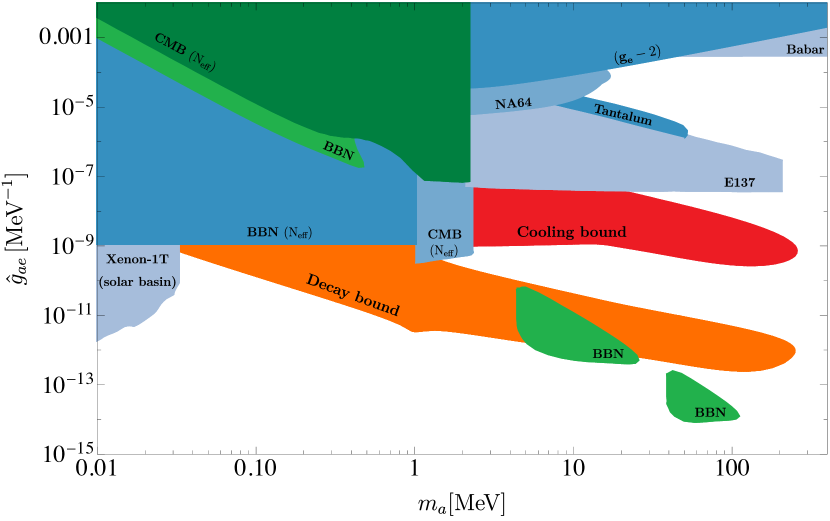
Figure 10: Compilation of laboratory, astrophysical and cosmological bounds on $\hat{g}_{ae}$. The bounds derived in this work are the SN bounds in orange and red, and the cosmological bounds in green. The remaining bounds (blue) were taken from [15, 65, 66, 67, 68, 69, 70, 20] (see main text for more details). Note that $\hat{g}_{ae}$ in units of $\operatorname{MeV}^{-1}$ is approximately equal to $g_{ae}$, see footnote 1 on footnote 1.

Laboratory bounds

The most competitive laboratory bounds on $\hat{g}_{ae}$ for ALP masses between $0.01-300$ MeV are:

• Electron anomalous magnetic moment: A massive ALP coupled to electrons contributes to the anomalous magnetic moment $a_{e}=(g_{e}-2)/2$ of the electron at one-loop level as $\Delta a_{e}\approx\hat{g}_{ae}m_{e}^{4}/(2m_{a}^{2}\pi^{2})\left(2\log(m_{a}/m_{e})-11/6\right)$ for $m_{a}\gg m_{e}$ [33]. The experimental bound $\Delta a_{e}<9.8\cdot 10^{-13}$ reported by [69] can then be translated into a bound on $\hat{g}_{ae}$.

• Xenon1T: The underground Xenon1T detector is sensitive to the local density of weakly interacting particles coupled to electrons [71, 72]. Massive ALPs produced in the sun via the $\hat{g}_{ae}$ coupling can accumulate in gravitationally bound orbits around the sun and yield a density that can be constrained with Xenon1T [65].

• Tantalum target: The authors of [73] reported the data analysis of a $45$ MeV electron beam hitting a tantalum target. ALPs produced by electron Bremsstrahlung could decay into electrons and positrons and be detected by the Sodium crystals. We report the bound on $\hat{g}_{ae}$ obtained in [66].

• Babar: Searches from the Babar experiment ($e^{+}e^{-}$ collider) at the PEP-II B-factory [74] for single photon events with missing energy. We report the constraint on $\hat{g}_{ae}$ from the analysis in [67].

• Beam Dumps: Searches for neutral particles produced by electron/proton beams that decayed into electron-positron pairs or led to missing energy:

  • NA64: 100 GeV electron beam at CERN SPS H4 [68].

  • E137: 20 GeV electron beam at SLAC [75, 70].

Cosmological bounds

We now turn to bounds on $\hat{g}_{ae}$ obtained from cosmological data. ALPs will inevitably be produced in the primordial plasma via their coupling to electrons or the (loop-induced) coupling to photons. Therefore, even if their initial abundance, here considered to be at temperatures around $10$ GeV [20], is negligible, they can affect cosmological observables in several ways. We will separate the discussion in two parts depending on whether the ALPs are produced in the primordial plasma mostly via scatterings with electrons or via inverse decays of electron-positron pairs or photons.

Production via scatterings: ALPs described by equation 2.1 can be produced in the primordial plasma via electron-positron ($e^{-}e^{+}\to a\,\gamma$) and Compton ($e^{\pm}\gamma\to a\,e^{\pm}$) scatterings at a rate proportional to $\hat{g}_{ae}^{2}$. At the time of big bang nucleosynthesis (BBN), the resulting ALP abundance will contribute to the effective number of relativistic degrees of freedom, $N_{\text{eff}}$, that is well constrained during that epoch to be $N_{\text{eff}}^{\text{BBN}}<3.43$ at 95% C.L. [76].

In order to derive a constraint on $\hat{g}_{ae}$ from the bound on $N_{\text{eff}}$, we computed the scattering cross-sections for massive ALPs (see appendix A). We then performed the thermal average and solved the Boltzmann equation for the ALP abundance following the steps described in [77, 78]. We stopped the Boltzmann equation at neutrino decoupling ($T\simeq 2$ MeV) and translated the ALP abundance into $N_{\text{eff}}^{\text{BBN}}$ (see [77, 78] for more details). Imposing the observational bound on $N_{\text{eff}}^{\text{BBN}}$ yields the blue region labelled BBN $(N_{\text{eff}})$ in figure 10. Our results are in good agreement with those obtained in [15]. Note that we restricted ourselves to the range $m_{a}<2m_{e}$: for heavier ALPs the production via inverse decays is more efficient and the discussion in the next paragraph holds.

Production via inverse decays: ALPs that decay to Standard Model particles after BBN can: i) photodisintegrate light nuclei and affect their primordial abundances [79, 20]; ii) heat the plasma after neutrinos have decoupled thus effectively decreasing $N_{\text{eff}}$ at the time of CMB formation [20].

A recent analysis constrained the decay rate of ALPs to electron-positron pairs, using the Planck constraint on $N_{\text{eff}}$, and to photons, using the Planck constraint on $N_{\text{eff}}$ and the measurements of primordial abundances [20]. The former can be directly translated into constraints on $\hat{g}_{ae}$ (dark green region labelled CMB $(N_{\text{eff}})$ in figure 10). For the latter, even if the ALPs do not couple at tree-level to photons, they can decay via an electron-loop with the effective coupling $g_{a\gamma}^{\text{(D)}}\sim\hat{g}_{ae}$ as in equation 2.5a. Therefore, the Planck constraints on ALP-to-photon decays derived in [20] also put new bounds on $\hat{g}_{ae}$.. The excluded regions are shown in figure 10 in light and dark green, labelled BBN and CMB $(N_{\text{eff}})$ depending, respectively, on whether the constraints on $g_{a\gamma}^{\text{(D)}}$ come from measurements of the primordial abundances of light nuclei or from the Planck constraint on $N_{\text{eff}}$. For larger masses and smaller couplings, the production of ALPs is less efficient so there is a smaller ALP abundance after BBN. Nevertheless, for ALP masses above twice the threshold to disintegrate deuterium ($m_{a}>4.4$ MeV) and Helium-4 ($m_{a}>39.6$ MeV), the photons resulting from ALP decays can still significantly affect the abundance of deuterium thus giving rise to the two green exclusion islands in figure 10. Note that if an initial ALP abundance is assumed stronger bounds can be derived [80, 20].

Discussion of the bounds obtained

Figure 10 summarises the three different types of constraints on $\hat{g}_{ae}$ that we have discussed in this paper: the SN bounds derived in sections 4 and 5 (in red and orange); the cosmological bounds derived in this work and described in the previous paragraphs (in the two shades of green); and the laboratory and cosmological bounds that were already present in the literature and also listed in the beginning of this section (in blue shades). We will now compare the different bounds, and then discuss the model dependence of the SN bounds.

The analysis in [65], that used the data collected by the Xenon1T collaboration [71, 72], provides the strongest constraint on $\hat{g}_{ae}$ for ALP masses not far from the solar temperature ($m_{a}<30$ keV). The remaining laboratory bounds [66, 67, 70] provide competitive constraints on $\hat{g}_{ae}$ for $m_{a}>2m_{e}$ and exclude, in some regions, couplings larger than $\hat{g}_{ae}\gtrsim 4\times 10^{-8}$. The region constrained by ALP production from electron scatterings (region labelled BBN ($N_{\text{eff}}$), see also [15]) is competitive with the SN cooling bound for $m_{a}<2m_{e}$, however, it extends to much larger couplings. At those masses, larger couplings are further excluded by the possibility of decay to photons via equation 2.5a (regions labelled CMB ($N_{\text{eff}}$) and BBN). The region excluded by BBN also includes two islands at masses around $m_{a}\simeq 4-25$ and $m_{a}\simeq 40-110$ MeV and smaller values of the couplings, down to $\hat{g}_{ae}\simeq 10^{-14}$. Finally, the SN cooling and decay bounds derived in sections 4 and 5 constrain unique regions of parameter space, $m_{a}\simeq 2-250$ MeV and $m_{a}\simeq 0.03-240$ MeV, respectively, that span roughly four (two) orders of magnitude in the coupling in the case of the decay (cooling) bound.

In our analysis, we isolated the physical effects originating from the ALP-electron coupling and so neglected other possible signals that do not depend on $\hat{g}_{ae}$. However, in many ALP models the presence of couplings to other standard model fields or to a dark sector is expected. Therefore, it is instructive to discuss the model dependence of the SN bounds on $\hat{g}_{ae}$ derived in sections 4 and 5 (c.f. figure 8).

Additional couplings of the ALP to particles in the core of the SN (e.g. tree-level couplings to photons or nucleons) can have two different effects. First, they will make the production of ALPs more efficient. Therefore, the lower limit of the cooling bound derived in this work is conservative and generically model independent. Second, they will also make it harder for the ALPs that are produced to escape the SN. This will tend to decrease the upper limit of the cooling bound, the so-called trapping region. Conversely, the upper limit of the cooling bound will tend to increase if there are couplings that allow the luminosity stored in the ALPs to be converted into a dark sector before the ALP gets re-absorbed in the SN core.

For the decay bound, additional couplings to particles heavier than the ALP (e.g. nucleons) will only improve the constraint since more ALPs can be produced, but the decay length and the $a\to\gamma\gamma$ branching ratio in section 5 will not change. If, on the other hand, these particles are so light that the decay length of the ALP or the branching ratio of photon-decays will decrease, the upper end of the decay bound will be moved down to smaller couplings.

7 Conclusion

In this section, we conclude by summarising the main results obtained in this work, and by indicating a few directions for future research.

7.1 Summary of results

The most important result of this work is that the effective ALP-photon coupling at one loop, $g_{a\gamma}^{\text{eff}}$, is process-dependent (cf. equation 2.2). In the previous literature, the on-shell limit of this effective coupling, $g_{a\gamma}^{\text{(D)}}$, has been broadly used. While $g_{a\gamma}^{\text{(D)}}$ is appropriate for e.g. the radiative decay of ALPs into photons, it is not the correct coupling for processes involving one or more off-shell particles. For example, the Primakoff process involves one internal, off-shell photon and leads to an effective coupling, $g_{a\gamma}^{\text{(P)}}$, that differs qualitatively and quantitatively from $g_{a\gamma}^{\text{(D)}}$. While $g_{a\gamma}^{\text{(D)}}$ goes to zero as $m_{a}\to 0$, $g_{a\gamma}^{\text{(P)}}$ remains finite. While $g_{a\gamma}^{\text{(D)}}$ is momentum independent, $g_{a\gamma}^{\text{(P)}}$ depends on the Mandelstam $t$ variable. The difference between the couplings becomes particularly pronounced in hot and dense environments, such as that of a supernova.

Using a state-of-the-art supernova model [19], we have shown that quantum loops have strong implications for the predictions of ALP theories. There are new channels for ALP production at one loop (Primakoff and photon coalescence), and we showed that, due to the large temperature in the supernova core, these channels can be as efficient as the previously studied tree-level channels for ALP production. In a region of the parameter space, the ALPs can escape the supernova and carry substantial amounts of energy away from it. This excess cooling can be constrained using the duration of the neutrino burst from SN1987A [1]. We use this method to place a ‘cooling bound’ on $\hat{g}_{ae}$, that incorporates both tree-level and loop-level interactions. Finally, we derive a ‘decay bound’ on $\hat{g}_{ae}$ by including the one-loop decay into photons, which can be constrained by the absence of a gamma-ray burst associated with SN1987A [62].

Moreover, we have shown that one-loop processes lead to strong limits on $\hat{g}_{ae}$ by considering cosmological limits from the CMB and BBN, in particular on the primordial abundance of light elements. In sum, the constraints derived in this work are the leading constraints on the ALP-electron coupling in most of the mass range $0.03\text{ MeV}<m_{a}<240\text{ MeV}$.

Finally, we have also corrected and improved some technical aspects in the literature, such as including quantum statistics in the absorption processes in section 4.1, which is important in the hot and degenerate supernova core, or improving the analysis of the probability of photon detection from ALP decays in section 5.

7.2 Outlook

There are several possible interesting extensions of this work.

With the formulas for the differential fluence of gamma-rays in equation 5.1, and the calculations of the ALP production spectra for photon coalescence and the Primakoff effect (with $m_{a}>0$) we can derive the ‘decay bound’ of section 5 for an ALP with tree-level couplings to photons. This would amount to an update of [62] (and an extension of section 5C in [40] to larger masses).

Recently, it has been pointed out that when the ALP decays quickly, the energy deposition in the progenitor star of low-energy core collapse supernovae can be large enough to affect their explosion kinematics [81, 57]. A natural extension of our work would be to study how this additional effect can be used to constraint the ALP-electron coupling once the effective coupling to photons is taken into account.

Furthermore, more distant supernovae than SN1987A are expected to contribute to a diffuse background of ALPs [82]. Such ALPs can convert into photons in astrophysical magnetic fields, which leads to an expected gamma-ray signal that can be searched for in data by e.g. Fermi-LAT [83]. In an extension of the ‘decay bound’ discussed in section 5 and the analysis in [82], it would be interesting to constrain the diffuse background of heavy ALPs through their loop-induced decays into photons.

Moreover, we have restricted our analysis to the case of supernovae. This was justified by the fact that the effective coupling of ALPs to photons takes the largest values in hot environments where the temperature can overcome the electron mass. However, it would be interesting to understand if the effective coupling to photons can still play a role in other hot environments such as the core of red giants [53] where temperatures can be as large as $10$ keV, or in the vicinity of low-luminosity black holes where the temperatures can also reach very large values [84].

In a broader context, the interplay between tree-level ALP-fermion couplings and loop-induced couplings to gauge fields is naturally not specific to electrons and photons. The case of light spin-0 particles coupled only to muons at tree-level was recently studied in [40]. It was assumed that the effective ALP-photon coupling induced by a derivative coupling to muons vanishes for $m_{a}\ll m_{\mu}\simeq 100$ MeV, but as we have shown in section 2 and discussed throughout this paper, this is not generally true and it would be interesting to re-consider the decay bound for large ALP masses in the light of our results.

We anticipate that the formalism developed and applied in this work will prove useful for future studies of astrophysical ALPs. Our work emphasises the important point that the effective couplings of ALPs are not arbitrary, but abide by quantum relations that make large hierarchies difficult to realise.

Appendix A Cross-sections for ALP production via electron Compton scattering and pair production

In this appendix we give the expressions for the cross-sections used in section 6 to compute the ALP abundance contribution to $\Delta N_{\text{eff}}$ at neutrino decoupling.

• Pair production:

  $$\sigma_{e^{-}+e^{+}\to a+\gamma}=4\alpha_{\text{EM}}\,\hat{g}_{ae}^{2}\,\frac{m_{e}^{2}}{s}\,\frac{\left(m_{a}^{4}-4m_{a}^{2}m_{e}^{2}+s^{2}\right)\tanh^{-1}\left(\sqrt{1-\frac{4m_{e}^{2}}{s}}\right)-m_{a}^{2}\sqrt{s\left(s-4m_{e}^{2}\right)}}{\left(s-4m_{e}^{2}\right)(s-m_{a}^{2})}$$

• Compton scattering:

  $$\sigma_{e^{\pm}\gamma\to e^{\pm}a}= \,\alpha_{\text{EM}}\,\hat{g}_{ae}^{2}\,\frac{m_{e}^{2}}{2s^{2}}\frac{\sqrt{m_{a}^{4}-2m_{a}^{2}\left(m_{e}^{2}+s\right)+\left(m_{e}^{2}-s\right)^{2}}}{\left(s-m_{e}^{2}\right)^{3}}\times$$

  $$\left(m_{a}^{2}\left(-m_{e}^{4}+2m_{e}^{2}s+7s^{2}\right)+\left(m_{e}^{2}-s\right)^{2}\left(m_{e}^{2}-3s\right)-\right.$$

  $$\left.\frac{4s^{2}\left(2m_{a}^{4}-2m_{a}^{2}\left(m_{e}^{2}+s\right)+\left(m_{e}^{2}-s\right)^{2}\right)\coth^{-1}\left(\frac{m_{a}^{2}-m_{e}^{2}-s}{\sqrt{m_{a}^{4}-2m_{a}^{2}\left(m_{e}^{2}+s\right)+\left(m_{e}^{2}-s\right)^{2}}}\right)}{\sqrt{m_{a}^{4}-2m_{a}^{2}\left(m_{e}^{2}+s\right)+\left(m_{e}^{2}-s\right)^{2}}}\right)$$

where we assumed $m_{a}<2m_{e}$ in both cases.

References

- [1] G. G. Raffelt, Stars as laboratories for fundamental physics: The astrophysics of neutrinos, axions, and other weakly interacting particles. University of Chicago Press, 5, 1996.
- [2] R. D. Peccei and H. R. Quinn, CP Conservation in the Presence of Instantons, Phys. Rev. Lett. 38 (1977) 1440–1443.
- [3] R. D. Peccei and H. R. Quinn, Constraints Imposed by CP Conservation in the Presence of Instantons, Phys. Rev. D 16 (1977) 1791–1797.
- [4] S. Weinberg, A New Light Boson?, Phys. Rev. Lett. 40 (1978) 223–226.
- [5] F. Wilczek, Problem of Strong and Invariance in the Presence of Instantons, Phys. Rev. Lett. 40 (1978) 279–282.
- [6] J. Preskill, M. B. Wise and F. Wilczek, Cosmology of the Invisible Axion, Phys. Lett. B 120 (1983) 127–132.
- [7] L. F. Abbott and P. Sikivie, A Cosmological Bound on the Invisible Axion, Phys. Lett. B 120 (1983) 133–136.
- [8] M. Dine and W. Fischler, The Not So Harmless Axion, Phys. Lett. B 120 (1983) 137–141.
- [9] P. Svrcek and E. Witten, Axions In String Theory, JHEP 06 (2006) 051, [hep-th/0605206].
- [10] G. B. Gelmini and M. Roncadelli, Left-Handed Neutrino Mass Scale and Spontaneously Broken Lepton Number, Phys. Lett. B 99 (1981) 411–415.
- [11] A. Davidson and K. C. Wali, MINIMAL FLAVOR UNIFICATION VIA MULTIGENERATIONAL PECCEI-QUINN SYMMETRY, Phys. Rev. Lett. 48 (1982) 11.
- [12] F. Wilczek, Axions and Family Symmetry Breaking, Phys. Rev. Lett. 49 (1982) 1549–1552.
- [13] N. Craig, A. Hook and S. Kasko, The Photophobic ALP, JHEP 09 (2018) 028, [1805.06538].
- [14] R. Z. Ferreira, M. C. D. Marsh and E. Müller, Do direct detection experiments constrain axionlike particles coupled to electrons?, 2202.08858.
- [15] D. Ghosh and D. Sachdeva, Constraints on Axion-Lepton coupling from Big Bang Nucleosynthesis, JCAP 10 (2020) 060, [2007.01873].
- [16] J. R. Ellis and K. A. Olive, Constraints on Light Particles From Supernova Sn1987a, Phys. Lett. B 193 (1987) 525.
- [17] G. Raffelt and D. Seckel, Bounds on Exotic Particle Interactions from SN 1987a, Phys. Rev. Lett. 60 (1988) 1793.
- [18] G. Lucente and P. Carenza, Supernova bound on axionlike particles coupled with electrons, Phys. Rev. D 104 (2021) 103007, [2107.12393].
- [19] T. Fischer, P. Carenza, B. Fore, M. Giannotti, A. Mirizzi and S. Reddy, Observable signatures of enhanced axion emission from protoneutron stars, Phys. Rev. D 104 (2021) 103012, [2108.13726].
- [20] P. F. Depta, M. Hufnagel and K. Schmidt-Hoberg, Updated BBN constraints on electromagnetic decays of MeV-scale particles, JCAP 04 (2021) 011, [2011.06519].
- [21] M. Carena and R. D. Peccei, The Effective Lagrangian for Axion Emission From SN1987A, Phys. Rev. D 40 (1989) 652.
- [22] K. Choi, K. Kang and J. E. Kim, Invisible Axion Emissions From SN1987A, Phys. Rev. Lett. 62 (1989) 849.
- [23] J. Quevillon and C. Smith, Axions are blind to anomalies, Eur. Phys. J. C 79 (2019) 822, [1903.12559].
- [24] R. Mertig, M. Böhm and A. Denner, Feyn Calc - computer-algebraic calculation of feynman amplitudes, Computer Physics Communications 64 (1991) 345–359.
- [25] V. Shtabovenko, R. Mertig and F. Orellana, New Developments in FeynCalc 9.0, Comput. Phys. Commun. 207 (2016) 432–444, [1601.01167].
- [26] V. Shtabovenko, R. Mertig and F. Orellana, FeynCalc 9.3: New features and improvements, Comput. Phys. Commun. 256 (2020) 107478, [2001.04407].
- [27] H. H. Patel, Package-X: A Mathematica package for the analytic calculation of one-loop integrals, Comput. Phys. Commun. 197 (2015) 276–290, [1503.01469].
- [28] T. Hahn and M. Perez-Victoria, Automatized one loop calculations in four-dimensions and D-dimensions, Comput. Phys. Commun. 118 (1999) 153–165, [hep-ph/9807565].
- [29] G. Passarino and M. J. G. Veltman, One Loop Corrections for e+ e- Annihilation Into mu+ mu- in the Weinberg Model, Nucl. Phys. B 160 (1979) 151–207.
- [30] G. ’t Hooft and M. J. G. Veltman, Scalar One Loop Integrals, Nucl. Phys. B 153 (1979) 365–401.
- [31] P. Breitenlohner and D. Maison, Dimensional Renormalization and the Action Principle, Commun. Math. Phys. 52 (1977) 11–38.
- [32] G. ’t Hooft and M. J. G. Veltman, Regularization and Renormalization of Gauge Fields, Nucl. Phys. B 44 (1972) 189–213.
- [33] M. Bauer, M. Neubert, S. Renner, M. Schnubel and A. Thamm, Flavor probes of axion-like particles, 2110.10698.
- [34] M. Chala, G. Guedes, M. Ramos and J. Santiago, Running in the ALPs, Eur. Phys. J. C 81 (2021) 181, [2012.09017].
- [35] M. Bauer, M. Neubert, S. Renner, M. Schnubel and A. Thamm, The Low-Energy Effective Theory of Axions and ALPs, JHEP 04 (2021) 063, [2012.12272].
- [36] M. D. Schwartz, Quantum Field Theory and the Standard Model. Cambridge University Press, 3, 2014.
- [37] S. Weinberg, The quantum theory of fields. Vol. 2: Modern applications. Cambridge University Press, 8, 2013.
- [38] M. Bauer, M. Neubert and A. Thamm, Collider Probes of Axion-Like Particles, JHEP 12 (2017) 044, [1708.00443].
- [39] L. Calibbi, D. Redigolo, R. Ziegler and J. Zupan, Looking forward to Lepton-flavor-violating ALPs, 2006.04795.
- [40] A. Caputo, G. Raffelt and E. Vitagliano, Muonic boson limits: Supernova redux, Phys. Rev. D 105 (2022) 035022, [2109.03244].
- [41] A. Payez, C. Evoli, T. Fischer, M. Giannotti, A. Mirizzi and A. Ringwald, Revisiting the SN1987A gamma-ray limit on ultralight axion-like particles, JCAP 02 (2015) 006, [1410.3747].
- [42] G. Lucente, P. Carenza, T. Fischer, M. Giannotti and A. Mirizzi, Heavy axion-like particles and core-collapse supernovae: constraints and impact on the explosion mechanism, JCAP 12 (2020) 008, [2008.04918].
- [43] F. Ertas and F. Kahlhoefer, On the interplay between astrophysical and laboratory probes of MeV-scale axion-like particles, JHEP 07 (2020) 050, [2004.01193].
- [44] R. P. Brinkmann and M. S. Turner, Numerical Rates for Nucleon-Nucleon Axion Bremsstrahlung, Phys. Rev. D 38 (1988) 2338.
- [45] P. Carenza, T. Fischer, M. Giannotti, G. Guo, G. Martínez-Pinedo and A. Mirizzi, Improved axion emissivity from a supernova via nucleon-nucleon bremsstrahlung, JCAP 10 (2019) 016, [1906.11844].
- [46] R. Bollig, W. DeRocco, P. W. Graham and H.-T. Janka, Muons in Supernovae: Implications for the Axion-Muon Coupling, Phys. Rev. Lett. 125 (2020) 051104, [2005.07141].
- [47] A. Mezzacappa and S. W. Bruenn, A numerical method for solving the neutrino Boltzmann equation coupled to spherically symmetric stellar core collapse, Astrophys. J. 405 (1993) 669–684.
- [48] M. Liebendoerfer, O. E. B. Messer, A. Mezzacappa, S. W. Bruenn, C. Y. Cardall and F. K. Thielemann, A Finite difference representation of neutrino radiation hydrodynamics for spherically symmetric general relativistic supernova simulations, Astrophys. J. Suppl. 150 (2004) 263–316, [astro-ph/0207036].
- [49] T. Fischer, M. Hempel, I. Sagert, Y. Suwa and J. Schaffner-Bielich, Symmetry energy impact in simulations of core-collapse supernovae, Eur. Phys. J. A 50 (2014) 46, [1307.6190].
- [50] A. Betranhandy and E. O’Connor, Neutrino Driven Explosions aided by Axion Cooling in Multidimensional Simulations of Core-Collapse Supernovae, 2204.00503.
- [51] T. Fischer, S. Chakraborty, M. Giannotti, A. Mirizzi, A. Payez and A. Ringwald, Probing axions with the neutrino signal from the next galactic supernova, Phys. Rev. D 94 (2016) 085012, [1605.08780].
- [52] G. G. Raffelt, Astrophysical methods to constrain axions and other novel particle phenomena, Phys. Rept. 198 (1990) 1–113.
- [53] P. Carenza and G. Lucente, Revisiting axion-electron bremsstrahlung emission rates in astrophysical environments, Phys. Rev. D 103 (2021) 123024, [2104.09524].
- [54] E. Braaten, Neutrino Emissivity of an Ultrarelativistic Plasma from Positron and Plasmino Annihilation, apj 392 (June, 1992) 70.
- [55] G. G. Raffelt, ASTROPHYSICAL AXION BOUNDS DIMINISHED BY SCREENING EFFECTS, Phys. Rev. D 33 (1986) 897.
- [56] A. Kopf and G. Raffelt, Photon dispersion in a supernova core, Phys. Rev. D 57 (1998) 3235–3241, [astro-ph/9711196].
- [57] A. Caputo, H.-T. Janka, G. Raffelt and E. Vitagliano, Low-Energy Supernovae Severely Constrain Radiative Particle Decays, Phys. Rev. Lett. 128 (2022) 221103, [2201.09890].
- [58] J. H. Chang, R. Essig and S. D. McDermott, Revisiting Supernova 1987A Constraints on Dark Photons, JHEP 01 (2017) 107, [1611.03864].
- [59] J. H. Chang, R. Essig and S. D. McDermott, Supernova 1987A Constraints on Sub-GeV Dark Sectors, Millicharged Particles, the QCD Axion, and an Axion-like Particle, JHEP 09 (2018) 051, [1803.00993].
- [60] A. Caputo, G. Raffelt and E. Vitagliano, Radiative transfer in stars by feebly interacting bosons, 2204.11862.
- [61] E. L. Chupp, W. T. Vestrand and C. Reppin, Experimental Limits on the Radiative Decay of SN1987A Neutrinos, Phys. Rev. Lett. 62 (1989) 505–508.
- [62] J. Jaeckel, P. C. Malta and J. Redondo, Decay photons from the axionlike particles burst of type II supernovae, Phys. Rev. D 98 (2018) 055032, [1702.02964].
- [63] A. H. Jaffe and M. S. Turner, Gamma-rays and the decay of neutrinos from SN1987A, Phys. Rev. D 55 (1997) 7951–7959, [astro-ph/9601104].
- [64] L. Oberauer, C. Hagner, G. Raffelt and E. Rieger, Supernova bounds on neutrino radiative decays, Astropart. Phys. 1 (1993) 377–386.
- [65] K. Van Tilburg, Stellar basins of gravitationally bound particles, Phys. Rev. D 104 (2021) 023019, [2006.12431].
- [66] A. A. Aguilar-Arevalo et al., Axion-Like Particles at Coherent CAPTAIN-Mills, 2112.09979.
- [67] L. Darmé, F. Giacchino, E. Nardi and M. Raggi, Invisible decays of axion-like particles: constraints and prospects, JHEP 06 (2021) 009, [2012.07894].
- [68] NA64 collaboration, Y. M. Andreev et al., Search for pseudoscalar bosons decaying into pairs in the NA64 experiment at the CERN SPS, Phys. Rev. D 104 (2021) L111102, [2104.13342].
- [69] L. Morel, Z. Yao, P. Cladé and S. Guellati-Khélifa, Determination of the fine-structure constant with an accuracy of 81 parts per trillion, Nature 588 (2020) 61–65.
- [70] R. Essig, R. Harnik, J. Kaplan and N. Toro, Discovering New Light States at Neutrino Experiments, Phys. Rev. D 82 (2010) 113008, [1008.0636].
- [71] XENON collaboration, E. Aprile et al., Light Dark Matter Search with Ionization Signals in XENON1T, Phys. Rev. Lett. 123 (2019) 251801, [1907.11485].
- [72] XENON collaboration, E. Aprile et al., Excess electronic recoil events in XENON1T, Phys. Rev. D 102 (2020) 072004, [2006.09721].
- [73] D. J. Bechis, T. W. Dombeck, R. W. Ellsworth, E. V. Sager, P. H. Steinberg, L. J. Teig et al., Search for Axion Production in Low-energy Electron Bremsstrahlung, Phys. Rev. Lett. 42 (1979) 1511.
- [74] BaBar collaboration, J. P. Lees et al., Search for Invisible Decays of a Dark Photon Produced in Collisions at BaBar, Phys. Rev. Lett. 119 (2017) 131804, [1702.03327].
- [75] J. D. Bjorken, S. Ecklund, W. R. Nelson, A. Abashian, C. Church, B. Lu et al., Search for Neutral Metastable Penetrating Particles Produced in the SLAC Beam Dump, Phys. Rev. D 38 (1988) 3375.
- [76] B. D. Fields, K. A. Olive, T.-H. Yeh and C. Young, Big-Bang Nucleosynthesis after Planck, JCAP 03 (2020) 010, [1912.01132].
- [77] R. Z. Ferreira and A. Notari, Observable Windows for the QCD Axion Through the Number of Relativistic Species, Phys. Rev. Lett. 120 (2018) 191301, [1801.06090].
- [78] F. D’Eramo, R. Z. Ferreira, A. Notari and J. L. Bernal, Hot Axions and the tension, JCAP 11 (2018) 014, [1808.07430].
- [79] M. Kawasaki, K. Kohri, T. Moroi and Y. Takaesu, Revisiting Big-Bang Nucleosynthesis Constraints on Long-Lived Decaying Particles, Phys. Rev. D 97 (2018) 023502, [1709.01211].
- [80] D. Cadamuro and J. Redondo, Cosmological bounds on pseudo Nambu-Goldstone bosons, JCAP 02 (2012) 032, [1110.2895].
- [81] A. Sung, H. Tu and M.-R. Wu, New constraint from supernova explosions on light particles beyond the Standard Model, Phys. Rev. D 99 (2019) 121305, [1903.07923].
- [82] F. Calore, P. Carenza, M. Giannotti, J. Jaeckel and A. Mirizzi, Bounds on axionlike particles from the diffuse supernova flux, Phys. Rev. D 102 (2020) 123005, [2008.11741].
- [83] F. Calore, P. Carenza, C. Eckner, T. Fischer, M. Giannotti, J. Jaeckel et al., 3D template-based -LAT constraints on the diffuse supernova axion-like particle background, 2110.03679.
- [84] A. Sadowski, M. Wielgus, R. Narayan, D. Abarca, J. C. McKinney and A. Chael, Radiative, two-temperature simulations of low luminosity black hole accretion flows in general relativity, Mon. Not. Roy. Astron. Soc. 466 (2017) 705–725, [1605.03184].