On the Difficulty of Defending Self-Supervised Learning against Model Extraction

On the Difficulty of Defending Self-Supervised Learning against Model Extraction(Supplement)

On the Difficulty of Defending Self-Supervised Learning against Model Extraction  (Supplement)

Abstract

Self-Supervised Learning (SSL) is an increasingly popular ML paradigm that trains models to transform complex inputs into representations without relying on explicit labels. These representations encode similarity structures that enable efficient learning of multiple downstream tasks. Recently, ML-as-a-Service providers have commenced offering trained SSL models over inference APIs, which transform user inputs into useful representations for a fee. However, the high cost involved to train these models and their exposure over APIs both make black-box extraction a realistic security threat. We thus explore model stealing attacks against SSL. Unlike traditional model extraction on classifiers that output labels, the victim models here output representations; these representations are of significantly higher dimensionality compared to the low-dimensional prediction scores output by classifiers. We construct several novel attacks and find that approaches that train directly on a victim’s stolen representations are query efficient and enable high accuracy for downstream models. We then show that existing defenses against model extraction are inadequate and not easily retrofitted to the specificities of SSL.

1 Introduction

Self-Supervised Learning (SSL) trains encoder models to transform unlabeled inputs into useful representations that are amenable to sample-efficient learning of multiple downstream tasks. The ability of SSL models to learn from unlabeled data has made them increasingly popular in important domains like computer vision, natural language processing, and speech recognition, where data are often abundant but labeling them is expensive (simclr; byol; moco; clip). Recently, ML-as-a-Service providers like OpenAI (neelakantan2022text; OpenAI) and Cohere (cohere) have begun offering trained encoders over inference APIs. Users pay a fee to transform their input data into intermediate representations, which are then used for downstream models. High-performance SSL models in these domains are often costly to train; training a large BERT model can cost north of 1 million USD (sharir2020cost). The value of these models and their exposure over publicly-accessible APIs make black-box model extraction attacks a realistic security threat.

In a model extraction attack (pred_apis), the attacker aims to steal a copy of the victim’s model by submitting carefully selected queries and observing the outputs. The attacker uses the query-output pairs to rapidly train a local model, often at a fraction of the cost of the victim model (fidelity). The stolen model can be used for financial gains or as a reconnaissance stage to mount further attacks like extracting private training data or constructing adversarial examples (papernot2017practical).

Past work on model extraction focused on the Supervised Learning (SL) setting, where the victim model typically returns a label or other low-dimensional outputs like confidence scores (pred_apis) or logits (DataFreeExtract). In contrast, SSL encoders return high-dimensional representations; the de facto output for a ResNet-50 SimCLR model, a popular architecture in vision, is a 2048-dimensional vector. We hypothesize this significantly higher information leakage from encoders makes them more vulnerable to extraction attacks than SL models.

In this paper, we introduce and compare several novel encoder extraction attacks to empirically demonstrate their threat to SSL models, and discuss the difficulties in protecting such models with existing defenses.

The framework of our attacks is inspired by Siamese networks: we query the victim model with inputs from a reference dataset similar to the victim’s training set (e.g. CIFAR10 against an ImageNet victim), and then use the query-output pairs to train a local encoder to output the same representations as the victim. We use two methods to train the local model during extraction. The first method directly minimizes the loss between the output layer of the local model and the output of the victim. The second method utilizes a separate projection head, which recreates the contrastive learning setup utilized by SSL frameworks like SimCLR. For each method, we compare different loss metrics, including MSE, InfoNCE, Soft Nearest Neighbors (SoftNN), or Wasserstein distance.

We evaluate our attacks against ResNet-50 and ResNet-34 SimCLR victim models. We train the models and generate queries for the extraction attacks using ImageNet and CIFAR10, and evaluate the models’ downstream performance on CIFAR100, STL10, SVHN, and Fashion-MNIST. We also simulate attackers with different levels of access to data that is in or out of distribution w.r.t. the victim’s training data.

Our experimental results in Section 4 show that our attacks can steal a copy of the victim model that achieves considerable downstream performance in fewer than $\nicefrac{{1}}{{5}}$ of the queries used to train the victim. Against a victim model trained on 1.2M unlabeled samples from ImageNet, with a 91.9% accuracy on the downstream Fashion-MNIST classification task, our direct extraction attack with the InfoNCE loss stole a copy of the encoder that achieves 90.5% accuracy in 200K queries. Similarly, against a victim trained on 50K unlabeled samples from CIFAR10, with a 79.0% accuracy on the downstream CIFAR10 classification task, our direct extraction attack with the SoftNN loss stole a copy that achieves 76.9% accuracy in 9,000 queries.

We discuss 5 current defenses against model extraction, including Prediction Poisoning (orekondy2019prediction), Extraction Detection (juuti2019prada), Watermarking (jia2020entangled), Dataset Inference (maini2021dataset), and Proof-of-Work (powDefense). We show that for each of these defenses, the existing implementations are inadequate in the SSL setting, and that retrofitting them to the specificities of encoders is non-trivial. We identify two main sources of this difficulty: the lack of labels and the higher information leakage from the model outputs.

Our main contributions are as follows:

• We call attention to a new setting for model extraction: the extraction of encoders trained with SSL. We find that the high dimensionality of their outputs make encoders particularly vulnerable to such attacks.

• We introduce and compare several novel model extraction attacks against SSL encoders and show that they are a realistic threat. In some cases, an attacker can steal a victim model using less than $\nicefrac{{1}}{{5}}$ of the queries required to train the victim.

• We discuss the effectiveness of existing defenses against model extraction in this new setting, and show that they are either inadequate or cannot be easily adapted for encoders. The difficulty stems from the lack of labels, which are utilized by some defenses, and the higher information leakage in the outputs compared to supervised models. We propose these challenges as avenues for future research.

2 Background and Related Work

2.1 Self-Supervised Learning

Self-Supervised Learning (SSL) is an ML paradigm that trains models to learn generic representations from unlabeled data. The representations are then used by downstream models to solve specific tasks. The training signal for SSL tasks is derived from an implicit structure in the input data, rather than explicit labels. For example, some tasks include predicting the rotation of an image (gidaris2018unsupervised), or predicting masked words in a sentence (devlin2018bert). These tasks teach models to identify key semantics of their input data and learn representations that are generally useful to many downstream tasks due to their similarity structure. Contrastive learning is a common approach to SSL where one trains representations so that similar pairs have representations close to each other while dissimilar ones are far apart.

2.2 Self-Supervised Learning Frameworks

Many new SSL frameworks have been proposed over the recent years; for ease of exposition, we focus on three current popular methods in the vision domain.

The SimCLR (simclr) framework learns representations by maximizing agreement between differently augmented views of the same sample via a contrastive InfoNCE loss (cpc) in the latent space. The architecture is a Siamese network that contains two encoders with shared weights followed by a projection head. During training, the encoders are fed either two augmentations of the same input (positive pair) or augmentations of different inputs (negative pair). The output representations of the encoders are then fed into the projection head, whose outputs are used to compute a distance in the latent space; positive pairs should be close, and negative pairs far. The encoders and the projection head are trained concurrently. The authors show that the crucial data augmentation to create positive samples and achieve strong performance is a combination of a random resized crop and color distortion.

SimSiam (SimSiam) is another Siamese network architecture that utilizes contrastive learning like SimCLR but simplifies the training process and architecture. In SimCLR, negative samples are needed during training to prevent the model from collapsing to a trivial solution, i.e. outputting the same representation for all inputs. The authors of SimSiam show that negative samples are not necessary; collapse can be avoided by applying the projection head to only one of the encoders (in alternation) and preventing the gradient from propagating through the other encoder during training.

Barlow Twins (zbontar2021barlow) aims to create similar representations of two augmentations of the same image while reducing redundancy between the output units of the representations. It measures the cross-correlation matrix between two views and optimizes the matrix to be close to the identity matrix. The optimization process uses a unique loss function involving an invariance term and a redundancy reduction term. As with other methods, a projection head is used before passing the representation to the loss function.

2.3 Model Extraction Attacks

In the model extraction attacks for SL, an attacker queries the victim model to label its training points (pred_apis). The main goals of such an adversary are to achieve a certain task accuracy of the stolen model (orekondy2019knockoff) or recreate a high fidelity copy that can be used to mount other attacks (fidelity), such as the construction of adversarial examples (szegedy2013intriguing; papernot2017practical). The attacker wants to minimize the number of queries required to achieve a given goal. In the self-supervised setting, the goal of an adversary is to learn high-quality embeddings that can be used to achieve high performance on many downstream tasks.

2.4 Defenses against Model Extraction

Defenses against model extraction can be categorized based on when they are applied in the extraction process. They can be classified as proactive, active, passive, or reactive.

Proactive defenses prevent the model stealing before it happens. One of the methods is based on the concept of proof-of-work (powDefense), where the model API users have to expand some compute by solving a puzzle before they can read the desired model output. The difficulty of the puzzle is calibrated based on the deviation of a user from the expected behavior for a legitimate user.

Active defenses introduce small perturbations into model outputs to poison the training objective of an attacker (orekondy2019prediction) or truncate outputs (pred_apis), however, these active methods lower the quality of results for legitimate users.

Passive defenses try to detect an attack (juuti2019prada). Reactive defenses are post-hoc methods that are used to determine if a suspect model was stolen or not. The examples of such methods are watermarking (jia2020entangled), dataset inference (maini2021dataset), and Proof-of-Learning (PoL) (jia2021proof). The PoL method can be immediately applied to SSL since defenders can claim ownership of a model by showing proof of incremental updates from their SSL model training.

3 Extraction Methods

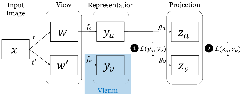
Figure 1: Stealing the encoder model $f_{v}$ using the direct comparison between victim and attacker’s representations or access to the latent vectors $z$ or recreating the projection head $g_{v}$.

3.1 Threat Model

The adversary makes queries to the victim model for representations of arbitrary inputs. The adversary has direct access only to the output representations. We consider settings where the adversary has/does not have knowledge about the encoder architecture, the victim’s data augmentation scheme, loss function used, victim’s training/test set or external dataset, and other parameters and hyper-parameters set by the victim during training of the encoder model.

3.2 Extraction Algorithms

We consider different approaches to extracting encoders trained with SSL. The final outcome of the self-supervised training process is an encoder or feature extractor $f$, where for an input $x$ we obtain the representation $y=f(x)$. The goal of an adversary is to steal the encoder $f$. Figure 1 presents the stealing process from the attacker’s perspective. An input image $x$ is augmented using two separate operators $t$ and $t^{\prime}$ to obtain two correlated views $w=t(x)$ and $w^{\prime}=t^{\prime}(x)$. Here a view refers to a version of the image under a particular augmentation. Note that it is possible that $t(x)=x$ in the case when no augmentations are used and that $w=w^{\prime}$ when the same augmentation operator is used by the victim and attacker. The view $w$ is passed through the attacker’s encoder $f_{a}$ to obtain representation $y_{a}$ and $w^{\prime}$ is fed to the victim’s encoder $f_{v}$ which returns $y_{v}$. The representations can be further passed to the victim’s head $g_{v}$ or attacker’s $g_{a}$ to obtain latent vectors $z_{v}$ or $z_{a}$, respectively. To train the stolen encoder, our adversary adopts the methodology of Siamese networks, for example, SimSiam (SimSiam), where one of the branches is the victim’s encoder and the other is the attacker’s stolen local model. The attacker tries to train the stolen model to output representations as similar as possible to the victim encoder.

Direct Extraction.

The first plain attack method directly steals the encoder $f$ by comparing the victim representation $y_{v}$ with the representation $y_{a}$ obtained on the attacker’s end through an appropriate loss function such as Mean Squared Error (MSE) or InfoNCE (cpc). Algorithm 1 presents the pseudo-code for stealing the representation model using the direct extraction method.

Algorithm 1 Stealing an Encoder.

Input: Querying Dataset $\mathcal{D}$, access to a victim model $f_{v}(w;\theta_{v})$.

Output: Stolen representation model $f_{a}(w;\theta_{a})$

1:  Initialize $f_{a}$ with a similar architecture as $f_{v}$.

2:  for sampled queries $\{x_{k}\}_{k=1}^{N}\in\mathcal{D}$ do

3:     Sample augmentations $t$ and $t^{\prime}$.

4:     Generate views $w_{k}=t(x_{k})$ and $w_{k}^{\prime}=t^{\prime}(x_{k})$.

5:     Query victim model to obtain representations:
$y_{v}=f_{v}(w_{k}^{\prime})$

6:     Generate representations from stolen model:
$y_{a}=f_{a}(w_{k})$

7:     Compute loss $\mathcal{L}\left\{y_{v},y_{a}\right\}$.

8:     Update stolen model parameters $\theta_{a}\coloneqq\theta_{a}-\eta\nabla_{\theta_{a}}\mathcal{L}$.

9:  end for

Recreate Projection Head. The projection head $g$ is a critical component in the training process used for many contrastive learning approaches as shown by simclr. However, it is usually discarded after the training process. Another method of stealing a model is thus to first recreate the victim’s head and then pass the representations obtained from the victim through the head before finding the loss (see the pseudo-code in Algorithm 2). In practice, recreating the head requires knowledge of the victim’s training process such as the augmentations and the loss function used which may not be possible in all cases. At the end of the attack spectrum, we also assess the case where the victim releases the projected representations $z$ or an adversary can access the head $g_{v}$.

Our adopted methodology is the Direct Extraction method since, as we show in the evaluation, this method is able to outperform or match the performance of more sophisticated methods such as the head recreation. Moreover, compared to these more sophisticated methods, which require the use of augmentations, direct extraction is less prone to being detected by a defender (as we discuss in Section LABEL:sec:detection-defense).

Algorithm 2 Recreating a Projection Head.

Input: Querying dataset $\mathcal{D}$, access to a victim model $f_{v}(w;\theta_{v})$.

Output: Recreated victim head $g_{v}(y;\theta_{v}^{\prime})$ as $g_{a}(y;\theta_{a}^{\prime})$.

1:  for sampled queries $\{x_{k}\}_{k=1}^{N}\in\mathcal{D}$ do

2:     Sample augmentations $t$ and $t^{\prime}$.

3:     Generate views $w_{k}=t(x_{k})$ and $w_{k}^{\prime}=t^{\prime}(x_{k})$.

4:     Query victim model to obtain representations:
$y_{k}=f_{v}(w_{k})$ and $y_{k}^{\prime}=f_{v}(w_{k}^{\prime})$.

5:     Pass representations through head: $z_{k}=g_{a}(y_{k})$ and $z_{k}^{\prime}=g_{a}(y_{k}^{\prime})$.

6:     Compute loss $\mathcal{L}\left\{z_{k},z_{k}^{\prime}\right\}$.

7:     Update parameters of the head $\theta_{a}^{\prime}\coloneqq\theta_{a}^{\prime}-\eta\nabla_{\theta_{a}^{\prime}}\mathcal{L}$.

8:  end for

3.3 Loss Functions

One of the most important hyper-parameter choices for representation stealing is the loss function, which can be categorized into quadratic, symmetrized, contrastive, and supervised-contrastive. They can be arranged into a hierarchy as in Figure LABEL:fig:loss-hierarchy. The standard quadratic loss like MSE (Mean Squared Error) can be used to directly compare the representations from the victim and the stolen copy. For example, we train a stolen copy of the model with the MSE objective such that it minimizes the $\ell_{2}$-distance between its predicted representations and the representation outputs from the victim model.

The symmetrized losses (byol; SimSiam), have two parts to the loss for a given data point $x$. When considering two separate views of $x$, $w$ and $w^{\prime}$, the first part of the loss is $\mathcal{L}_{1}(g(f(w)),f(w^{\prime}))$, where $f$ is the feature extractor, and $g$ represents the prediction head, which transforms the output of one view and matches it to the other view. More simply, the head $g$ is a small fully-connected neural network which transforms the representations from one space to another. The symmetry is achieved by computing the other part of the loss $\mathcal{L}_{2}(g(f(w^{\prime})),f(w))$ and the final symmetrized loss is $\mathcal{L}=\mathcal{L}_{1}+\mathcal{L}_{2}$. The loss functions $\mathcal{L}_{1}$ and $\mathcal{L}_{2}$ are commonly chosen as to be the negative cosine similarity. The standard supervised and symmetrized losses take into account only the distances between the representations and compare solely positive examples, i.e., the representations for the same input image.

Finally, modern batch contrastive approaches, such as InfoNCE (cpc) or Soft Nearest Neighbor (SoftNN) (softNearestNeighborLoss) compare not only positive but also the negative pair samples in terms of their distances and learn representations so that positive pairs have similar representations while negative pairs have representations which are far apart. The supervised contrastive loss (SupCon loss) (supconloss) is a novel extension to contrastive loss functions which uses labels from supervised learning in addition to positive and negative labeling. An attacker can use a labeled public dataset, such as ImageNet or Pascal VOC, to obtain the labels to be used with the SupCon loss.

4 Empirical Evaluation

4.1 Experimental Setup

We include results for victim models trained on the ImageNet, CIFAR10, and SVHN datatsets. The ImageNet encoder has an output representation dimension of 2048, while encoders trained on CIFAR10 and SVHN return 512 dimensional representations. For ImageNet, we use the publicly available ResNet50 model from (SimSiam). For the CIFAR10 and SVHN datasets, we use a public PyTorch implementation of SimCLR (simclr) to train victim ResNet18 and ResNet34 models over 200 epochs with a batch size of 256 and a learning rate of 0.0003 with the Cosine Annealing Scheduler and the Adam optimizer. For training stolen models, we use similar (hyper-)parameters to the training of the victim models. More details on the experimental setup are in Section LABEL:sec:exeperimental-setup-details.

4.2 Linear Evaluation

The usefulness of representations is determined by evaluating a linear layer trained from representations to predictions on a specific downstream task. We follow the same evaluation protocol as in simclr, where a linear prediction layer is added to the encoder and is fine-tuned with the full labeled training set from the downstream task while the rest of the layers of the network are frozen. The test accuracy is then used as the performance metric.

4.3 Methods of Model Extraction

We compare the stealing algorithms in Table 4.3. The Direct Extraction steals $f_{v}$ by directly comparing the victim’s and attacker’s representations using the SoftNN loss, the Recreate Head uses the SimSiam method of training to recreate the victim’s head which is then used for training a stolen copy, while Access Head trains a stolen copy using the latent vectors $z_{v}$ and the InfoNCE loss. For CIFAR10 and STL10 datasets, the Direct Extraction works best, while it is outperformed on the SVHN dataset by the Access Head method. The results for the Recreate Head are mixed; the downstream accuracy for loss functions such as InfoNCE improves when the head is first recreated while for other loss functions such as MSE, which directly compares the representations, the recreation of the head hurts the performance. This is in line with the SSL frameworks that use the InfoNCE loss on outputs from the heads (simclr). The results show that the representations can be stolen directly from the victim’s outputs; the recreation or access to the head is not critical for downstream performance.

We observe that bigger differences in performance stem from the selection of the loss function—a comparison of the different loss functions is found in Table 4.3. The choice of the loss function is an important parameter for stealing with the SoftNN stolen model having the highest downstream accuracy in two of the three datasets while InfoNCE has a higher performance in one of the tasks. However, as we show in Table LABEL:tab:combinednumqeury, the number of queries used is also a factor behind the performance of different loss functions. We note that the SupCon loss gives the best performance on the CIFAR10 downstream task and this is likely a result of the fact that SupCon assumes access to labeled query data, which in this case was the CIFAR10 test set.

The results in Table LABEL:tab:StealImagenet show the stealing of the encoder pre-trained on ImageNet. Most methods perform quite well in extracting a representation model at a fraction of the cost with a small number of queries (less than one fifth) required to train the victim model as well as augmentations not being required. In general, the Direct Extraction with InfoNCE loss performs the best and the performance of the stolen encoder increases with more queries.

Table 1: Comparison between attack methods for the classification top-1 accuracy on downstream tasks CIFAR10, STL10, and SVHN. The models are stolen from a CIFAR10 victim encoder with 9,000 queries from the CIFAR10 test set.

Method\Dataset	CIFAR10	STL10	SVHN
Victim Model	79.0	67.9	65.1
1-4 Direct Extraction	76.9	67.1	67.3
Recreate Head	59.9	52.8	56.3
Access Head	75.6	65.0	69.8

Table 2: Comparison between loss functions. We use the same setup as in Table 4.3. Loss functions with (*) use data augmentations.

Representations] ] [Passive (against contrastive losses) [Detect Similar Representations] ] [Reactive (against quadratic losses) [Watermarking Augmentations] [Dataset Inference from Representations] ] ]

Figure 4: Hierarchy of the defense methods.

A hierarchy of defense methods is presented in Figure 4.3.

Appendix D Stealing Algorithms

Algorithm 3 Training a Downstream Classifier for Linear Evaluation Protocol

Input: Victim or Stolen Model $f$, downstream task with labeled data

Output: Downstream linear classifier $g(x;\theta)$

1:  Add a linear layer to the model $f$ and freeze all previous layers

2:  for labeled query batches $\{x_{k},y_{k}\}_{k=1}^{N}$ do

3:    Compute loss $\mathcal{L}\left\{\{f(x_{k}),y_{k}\}\right\}$ where $\mathcal{L}\{f(x),y\}=-\sum_{i}y_{k}\log f(x)$

4:    Update linear model parameters $\theta\coloneqq\theta-\eta\nabla_{\theta}\mathcal{L}$

5:  end for

Appendix E Defenses

E.1 Prediction Poisoning

We can consider the gradient of the loss with respect to the model parameters $\theta\in\mathbb{R}^{D}$ for a query $x$ made by the attacker to formalize this objective as in (orekondy2019prediction). We let $y_{v}\in\mathbb{R}^{n}$ be the representations returned by the victim model and $\tilde{y_{v}}$ be the perturbed representations which will act as targets for the stolen model $F$ to be trained by the attacker. Then the gradient of the loss function which will be used by the attacker to update its model parameters based on the unperturbed representations is $a=-\nabla_{\theta}\mathcal{L}\{F(x;\theta),y_{v}\}$. Similarly, let $b=-\nabla_{\theta}\mathcal{L}\{F(x;\theta),\tilde{y_{v}}\}$ be the gradient when the perturbed representations are returned. To harm the attacker’s gradient, the similarity between $a$ and $b$ should be minimized. This similarity can be quantified with various metrics such as the $\ell_{2}$ distance or cosine similarity. We let $G$ be the downstream linear classifier trained by a legitimate user and $\phi\in\mathbb{R}^{E}$ be the parameters of this model. Further, let $J$ be the loss function used to train this classifier and $t\in\mathbb{R}^{k}$ be the target labels from the dataset used for the downstream task. Then in order to avoid harming the legitimate user, the victim must maximize the similarity between

$$c=-\nabla_{\phi}J\{G(y_{v};\phi),t\}$$

and

$$d=-\nabla_{\phi}J\{G(\tilde{y_{v}};\phi),t\}$$

Although there are various loss functions $\mathcal{L}$ which can be used by an attacker when training a stolen model, we assume for simplicity that the attacker uses the Mean Squared Error (MSE) loss. For the downstream task which involves a standard training task, we assume standard training so that $J$ can be chosen to be the Cross Entropy Loss. With these assumptions, $a$ can be simplified as:

$$-\nabla_{\theta}\mathcal{L}\{F(x;\theta),y_{v}\}$$

$$=-\nabla_{\theta}\frac{1}{n}\sum_{i=1}^{n}(F(x;\theta)_{i}-y_{v_{i}})^{2}$$

$$=-\frac{1}{n}\sum_{i=1}^{n}\nabla_{\theta}(F(x;\theta)_{i}-y_{v_{i}})^{2}$$

$$=-\frac{1}{n}\sum_{i=1}^{n}2(F(x;\theta)_{i}-y_{v_{i}})\nabla_{\theta}(F(x;\theta)_{i}-y_{v_{i}})$$

$$=-\frac{2}{n}\sum_{i=1}^{n}(F(x;\theta)_{i}-y_{v_{i}})\cdot\nabla_{\theta}(F(x;\theta)_{i})$$

since $\nabla_{\theta}y_{v}=0$. This can then be simplified as the matrix product

$$a=-\frac{2}{n}\nabla_{\theta}F^{T}(F(x;\theta)-y_{v})$$

where $\nabla_{\theta}F\in\mathbb{R}^{n\times D}$ is the Jacobian of the stolen model $F$. In a similar way, $b$ can be simplified to

$$b=-\frac{2}{n}\nabla_{\theta}F^{T}(F(x;\theta)-\tilde{y_{v}})$$

To optimize $\tilde{y_{v}}$ so that the similarity between $a$ and $b$ is minimized, we thus need to recreate the attacker’s model $F$ in some form to approximate the Jacobian $\nabla_{\theta}F$ and the model’s output $F(x)$. This can be done by using a surrogate model $F_{surr}$ on the victim’s end. Then if we let $\mathrm{sim}$ be the similarity function used, the optimization objective can be written as

$$\min_{\tilde{y_{v}}}\mathrm{sim}(a,b)=\min_{\tilde{y_{v}}}\mathrm{sim}(-\frac{2}{n}\nabla_{\theta}F_{surr}^{T}(F_{surr}(x;\theta)-y_{v}),-\frac{2}{n}\nabla_{\theta}F_{surr}^{T}(F_{surr}(x;\theta)-\tilde{y_{v}}))$$

We also simplify $c$ as

$$-\nabla_{\phi}J\{G(y_{v};\phi),t\}$$

$$=-\nabla_{\phi}-\sum_{i=1}^{k}t_{i}\log G(y_{v};\phi)_{i}$$

$$=\sum_{i=1}^{k}\nabla_{\phi}t_{i}\log G(y_{v};\phi)_{i}$$

$$=\sum_{i=1}^{k}t_{i}\nabla_{\phi}\log G(y_{v};\phi)_{i}$$

$$=\nabla_{\phi}\log G(y_{v})^{T}t$$

and $d$ as $\nabla_{\phi}\log G(\tilde{y_{v}})^{T}t$. In this case, we note that to satisfy this optimization requirement, the victim must recreate the downstream classifier $G$ to estimate the Jacobians $\nabla_{\phi}\log G(y_{v};\phi)\in\mathbb{R}^{k\times E}$ and $\nabla_{\phi}\log G(\tilde{y_{v}};\phi)$. Again this can be done using a surrogate model $G_{surr}$ on the victim’s end based on which we can write the optimization objective for the downstream task as

$$\max_{\tilde{y_{v}}}\mathrm{sim}(\nabla_{\phi}\log G_{surr}(y_{v})^{T}t,\nabla_{\phi}\log G_{surr}(\tilde{y_{v}})^{T}t)$$

We note that different similarity functions may be used for the two objectives. Therefore applying prediction poisoning requires a double optimization problem to be solved, each of which requires certain assumptions such as the type of loss function used.

E.2 Watermarking Defense

We include additional results for our Watermarking defense which embeds predictive information about a particular augmentation (rotations, in our case) in the features learned by the victim. The ability of the watermark to transfer is measured by the Watermark Success Rate, which is the accuracy of a classifier trained to predict the watermarking augmentation. In our experiments, this task is prediction between images rotated by angles in $[0^{\circ},180^{\circ}]$ or $[180^{\circ},360^{\circ}]$. A random, genuinely but separately trained, model achieves random performance on this task, i.e. around 50% watermark success rate. Table LABEL:tab:watermarking shows that the watermark transfers sufficiently for models stolen with SVHN queries and different losses. Since the watermarking strategy is closely related to the augmentations used during training or stealing, we test the watermark success rate for CIFAR10 queries that are augmented with the standard SimCLR augmentations, standard augmentations with rotations included, or no augmentations at all. We report these results in Table LABEL:tab:watermarking_cifar_aug and find that in all cases, the watermark transfers to the stolen model well. If the adversary happens to use rotations as an augmentation, the watermark transfer is significantly stronger. However, this is not necessary for good watermark transfer, as demonstrated by the NoAug success rates.

E.3 Dataset Inference Defense

We also tested an approach based on Dataset Inference (maini2021dataset) as a possible defense. In the case of representation models, we directly measure the $\ell_{2}$ distance between the representations of a victim model and a model stolen with various methods. We also compute the distance between the representations of a victim model and a random model, which in this case was trained on the same dataset and using the same architecture but a different random seed that resulted in different parameters. The distance is evaluated on the representations of each model on the training data used to train the victim model. We obtain the results averaged across the datasets in Table 18. The general trend is that the more queries the adversaries issue against the victim model that are used to train the stolen copy, the smaller the distance between the representations from the victim and stolen models. In terms of loss functions, the stealing with MSE always results in smaller distances than for another Random model. On the other hand, for attacks that use either InfoNCE or SoftNN losses, it is rather hard to differentiate between stolen models and a random model based on the distances of their representations from the victim as some have a higher distance while others have a lower distance. We also observe a similar trend with watermarks where the MSE and SoftNN loss methods give different performances compared to a random model.

The more an adversary interacts with the victim model to steal it, the easier it is to claim ownership by distinguishing the stolen model’s behavior on the victim model’s training set.

Table 18: $\ell_{2}$ distances between the representation of a stolen model and a victim model. The Random column denotes model of the same architecture and training procedure like the victim model but with a different initial random seed. The Victim column designates the type of dataset used by the victim. The AdvData represents the data used by an adversary to steal the victim model.

# Queries	Victim	AdvData	Random	MSE	InfoNCE	SoftNN
9K	CIFAR10	CIFAR10	34.1	26.6	44	14.4
50K	CIFAR10	CIFAR10	34.1	14.6	40	12.8
50K	ImageNet	CIFAR10	65.8	25.2	36.2	119.6

Table 19: Dataset Inference. Compare the differences between raw data points and their augmentations for different private and public datasets. We use statistical t-test where the null hypothesis is that the differences in distances are smaller for the public dataset than for the private dataset, where $\Delta\mu$ is the effect size. Size is the image size. U is un-/self-supervised learning, while S denotes the supervised learning.

Size	# Queries	# Aug.	Model	Learning	Private	Public	$\Delta\mu$	p-value	t-value
32	100	100	SVHN	U	SVHN	SVHN	-0.17	0.99	-2.90
32	10000	100	SVHN	U	SVHN	SVHN	-0.005	0.79	-0.82
224	64	10	ImageNet	U	ImageNet	ImageNet	-0.005	0.99	-2.53
224	32	10	ImageNet	S	ImageNet	ImageNet	0.71	0.028	1.92
224	64	10	ImageNet	S	ImageNet	ImageNet	1.06	$10^{-5}$	4.03
224	64	10	ImageNet	S	ImageNet	ImageNet	0.89	$10^{-4}$	3.61
224	128	10	ImageNet	S	ImageNet	ImageNet	0.36	0.02	1.97
224	256	10	ImageNet	S	ImageNet	ImageNet	-0.44	0.99	-3.31
224	256	10	ImageNet	S	ImageNet	ImageNet	-0.12	0.81	-0.87
224	1024	10	ImageNet	U	ImageNet	ImageNet	-0.02	1.0	-33.99
32	50	10	SVHN	S	SVHN	SVHN	0.15	0.0685	1.49
32	50	10	SVHN	S	SVHN	SVHN	0.39	0.033	1.84
32	50	10	CIFAR10	S	CIFAR10	CIFAR10	-0.46	0.99	-4.3

We present results for the dataset inference method in Table 19.

Appendix F Representation Model Architecture

This section shows a sample representation model architecture (in this case a ResNet34 model). (generated using torchsummary).

 

----------------------------------------------------------------

        Layer type               Output Shape         Param #

================================================================

            Conv2d-1           [-1, 64, 32, 32]           1,728

       BatchNorm2d-2           [-1, 64, 32, 32]             128

            Conv2d-3           [-1, 64, 32, 32]          36,864

       BatchNorm2d-4           [-1, 64, 32, 32]             128

            Conv2d-5           [-1, 64, 32, 32]          36,864

       BatchNorm2d-6           [-1, 64, 32, 32]             128

        BasicBlock-7           [-1, 64, 32, 32]               0

            Conv2d-8           [-1, 64, 32, 32]          36,864

       BatchNorm2d-9           [-1, 64, 32, 32]             128

           Conv2d-10           [-1, 64, 32, 32]          36,864

      BatchNorm2d-11           [-1, 64, 32, 32]             128

       BasicBlock-12           [-1, 64, 32, 32]               0

           Conv2d-13           [-1, 64, 32, 32]          36,864

      BatchNorm2d-14           [-1, 64, 32, 32]             128

           Conv2d-15           [-1, 64, 32, 32]          36,864

      BatchNorm2d-16           [-1, 64, 32, 32]             128

       BasicBlock-17           [-1, 64, 32, 32]               0

           Conv2d-18          [-1, 128, 16, 16]          73,728

      BatchNorm2d-19          [-1, 128, 16, 16]             256

           Conv2d-20          [-1, 128, 16, 16]         147,456

      BatchNorm2d-21          [-1, 128, 16, 16]             256

           Conv2d-22          [-1, 128, 16, 16]           8,192

      BatchNorm2d-23          [-1, 128, 16, 16]             256

       BasicBlock-24          [-1, 128, 16, 16]               0

           Conv2d-25          [-1, 128, 16, 16]         147,456

      BatchNorm2d-26          [-1, 128, 16, 16]             256

           Conv2d-27          [-1, 128, 16, 16]         147,456

      BatchNorm2d-28          [-1, 128, 16, 16]             256

       BasicBlock-29          [-1, 128, 16, 16]               0

           Conv2d-30          [-1, 128, 16, 16]         147,456

      BatchNorm2d-31          [-1, 128, 16, 16]             256

           Conv2d-32          [-1, 128, 16, 16]         147,456

      BatchNorm2d-33          [-1, 128, 16, 16]             256

       BasicBlock-34          [-1, 128, 16, 16]               0

           Conv2d-35          [-1, 128, 16, 16]         147,456

      BatchNorm2d-36          [-1, 128, 16, 16]             256

           Conv2d-37          [-1, 128, 16, 16]         147,456

      BatchNorm2d-38          [-1, 128, 16, 16]             256

       BasicBlock-39          [-1, 128, 16, 16]               0

           Conv2d-40            [-1, 256, 8, 8]         294,912

      BatchNorm2d-41            [-1, 256, 8, 8]             512

           Conv2d-42            [-1, 256, 8, 8]         589,824

      BatchNorm2d-43            [-1, 256, 8, 8]             512

           Conv2d-44            [-1, 256, 8, 8]          32,768

      BatchNorm2d-45            [-1, 256, 8, 8]             512

       BasicBlock-46            [-1, 256, 8, 8]               0

           Conv2d-47            [-1, 256, 8, 8]         589,824

      BatchNorm2d-48            [-1, 256, 8, 8]             512

           Conv2d-49            [-1, 256, 8, 8]         589,824

      BatchNorm2d-50            [-1, 256, 8, 8]             512

       BasicBlock-51            [-1, 256, 8, 8]               0

           Conv2d-52            [-1, 256, 8, 8]         589,824

      BatchNorm2d-53            [-1, 256, 8, 8]             512

           Conv2d-54            [-1, 256, 8, 8]         589,824

      BatchNorm2d-55            [-1, 256, 8, 8]             512

       BasicBlock-56            [-1, 256, 8, 8]               0

           Conv2d-57            [-1, 256, 8, 8]         589,824

      BatchNorm2d-58            [-1, 256, 8, 8]             512

           Conv2d-59            [-1, 256, 8, 8]         589,824

      BatchNorm2d-60            [-1, 256, 8, 8]             512

       BasicBlock-61            [-1, 256, 8, 8]               0

           Conv2d-62            [-1, 256, 8, 8]         589,824

      BatchNorm2d-63            [-1, 256, 8, 8]             512

           Conv2d-64            [-1, 256, 8, 8]         589,824

      BatchNorm2d-65            [-1, 256, 8, 8]             512

       BasicBlock-66            [-1, 256, 8, 8]               0

           Conv2d-67            [-1, 256, 8, 8]         589,824

      BatchNorm2d-68            [-1, 256, 8, 8]             512

           Conv2d-69            [-1, 256, 8, 8]         589,824

      BatchNorm2d-70            [-1, 256, 8, 8]             512

       BasicBlock-71            [-1, 256, 8, 8]               0

           Conv2d-72            [-1, 512, 4, 4]       1,179,648

      BatchNorm2d-73            [-1, 512, 4, 4]           1,024

           Conv2d-74            [-1, 512, 4, 4]       2,359,296

      BatchNorm2d-75            [-1, 512, 4, 4]           1,024

           Conv2d-76            [-1, 512, 4, 4]         131,072

      BatchNorm2d-77            [-1, 512, 4, 4]           1,024

       BasicBlock-78            [-1, 512, 4, 4]               0

           Conv2d-79            [-1, 512, 4, 4]       2,359,296

      BatchNorm2d-80            [-1, 512, 4, 4]           1,024

           Conv2d-81            [-1, 512, 4, 4]       2,359,296

      BatchNorm2d-82            [-1, 512, 4, 4]           1,024

       BasicBlock-83            [-1, 512, 4, 4]               0

           Conv2d-84            [-1, 512, 4, 4]       2,359,296

      BatchNorm2d-85            [-1, 512, 4, 4]           1,024

           Conv2d-86            [-1, 512, 4, 4]       2,359,296

      BatchNorm2d-87            [-1, 512, 4, 4]           1,024

       BasicBlock-88            [-1, 512, 4, 4]               0

         Identity-89                  [-1, 512]               0

           ResNet-90                  [-1, 512]               0

================================================================

Total params: 21,276,992

Trainable params: 21,276,992

Non-trainable params: 0

----------------------------------------------------------------

Input size MB: 0.01

Forward/backward pass size MB: 19.07

Params size MB: 81.17

Estimated Total Size MB: 100.25

----------------------------------------------------------------