Mondrian Forest for Data Stream Classification Under Memory Constraints

Abstract

Supervised learning algorithms generally assume the availability of enough memory to store data models during the training and test phases. However, this assumption is unrealistic when data comes in the form of infinite data streams, or when learning algorithms are deployed on devices with reduced amounts of memory. In this paper, we adapt the online Mondrian forest classification algorithm to work with memory constraints on data streams. In particular, we design five out-of-memory strategies to update Mondrian trees with new data points when the memory limit is reached. Moreover, we design node trimming mechanisms to make Mondrian trees more robust to concept drifts under memory constraints. We evaluate our algorithms on a variety of real and simulated datasets, and we conclude with recommendations on their use in different situations: the Extend Node strategy appears as the best out-of-memory strategy in all configurations, whereas different node trimming mechanisms should be adopted depending on whether a concept drift is expected. All our methods are implemented in the OrpailleCC open-source library and are ready to be used on embedded systems and connected objects.

1 Introduction

Supervised classification algorithms mostly assume the availability of abundant memory to store data and models. This is an issue when processing data streams — which are infinite sequences by definition — or when using memory-limited devices as is commonly the case in the Internet of Things. This paper studies how the Mondrian forest, a popular online classification method, can be adapted to work with data streams and memory constraints compatible with connected objects.

Although online and data stream classification methods both assume that the dataset is available as a sequence of elements, data stream methods assume that the dataset is infinite whereas online methods consider that it is large but still bounded in size. Consequently, online methods usually store the processed elements for future access whereas data stream methods do not.

Under memory constraints, a data stream classification model that has reached its memory limit faces two issues: (1) how to update the model when new data points arrive, which we denote as the out-of-memory strategy, and (2) how to adapt the model to concept drifts, i.e., changes in the learned concepts. The mechanisms described in this paper address these two issues in the Mondrian forest.

The Mondrian forest is a tree-based, ensemble, online learning method with comparable performance to offline Random Forest mondrian2014 . Previous experiments highlighted that Mondrian forest are sensitive to the amount of available memory khannouz2020 , which motivates their extension to memory-constrained environments. In practice, existing implementations mondrian_implementation_1 ; mondrian_implementation_2 of the Mondrian forest all assume enough memory and crash when memory is not available.

The concept drift is a common problem in data streams that occurs when the distribution of features changes throughout the stream. By design, the Mondrian forest is not equipped to adapt to concept drifts as its trees cannot be pruned, trimmed, or modified. When memory is saturated, this lack of adaptability to concept drift worsens as trees cannot even grow new branches to accommodate changes in feature distributions. Therefore, the Mondrian forest needs a mechanism to free memory such that new tree nodes can grow. Such a mechanism might also be useful for stable data streams as it would replace less accurate nodes with better performing ones.

In summary, this paper makes the following contributions:

1. We adapt the Mondrian forest for data streams;

2. We propose five new out-of-memory strategies for the Mondrian forest under memory constraints;

3. We propose three new node trimming mechanisms to make Mondrian forest adaptive to concept drifts;

4. We evaluate our strategies on six simulated and real datasets.

2 Materials and Methods

All the methods presented in this section are implemented in the OrpailleCC framework OrpailleCC . The scripts to reproduce our experiments are available on GitHub at https://github.com/big-data-lab-team/benchmark-har-data-stream.

2.1 Mondrian Forest

The Mondrian forest mondrian2014 is an ensemble method that aggregates Mondrian trees. Each tree in the forest recursively divides the feature space, similar to a traditional decision tree. However, the feature selected for the split and its corresponding value are chosen randomly rather than through an information gain metric. The probability to select a feature is based on the feature range, and the split value is uniformly chosen within the feature range. Unlike other decision trees, the Mondrian tree does not split leaves to introduce new nodes. Instead, it adds a new parent and sibling to the node where the split occurs, using the branch-out mechanism shown in Figure 1. The original node and its descendants remain unchanged, and only the data point that initialized the split is moved to the new sibling. The new parent contains a split that separates the original node and the new sibling. This approach enables the Mondrian tree to introduce new branches to internal nodes. The branch-out mechanism is randomly triggered when a data point falls outside of the node box, with a probability related to the distance between the new point and the node box. The training algorithm does not require labels to build the tree; however, each node maintains counters for each observed label. Therefore, labels can be delayed, but they are necessary for prediction. Furthermore, each node tracks the range of its feature, representing a box that contains all data points. A data point can create a new branch only if it belongs to a node and falls outside its box.

Figure 1: Illustration of the Mondrian tree before (top) and after (bottom) of a branch out. The left side shows the data points in a two-feature space with the node’s boxes and the splits. The right side shows the tree structure. The branch out is triggered by the purple data point.

2.2 Mondrian Forest for Data Stream Classification

The implementation of Mondrian forest presented in mondrian2014 ; mondrian_implementation_1 is online because trees rely on potentially all the previously seen data points to grow new branches. To support data streams, the Mondrian forest has to access data points only once as the dataset is assumed to be infinite in size. Algorithm 1, adapted from reference mondrian2014 , describes our data-stream implementation. Function update_box (line 11) updates the node’s box using the data point’s features. Function update_counters (line 12) updates the label counters assigned to the node. Function is_enough_memory (line 2) returns true if there is enough memory to run extend_tree (line 7). Function distance_to_box (line 3) compute the distance between a data point and the node’s box and it returns zero if the data point fall inside the box. Function random_bool (line 5) randomly select a boolean that is more likely to be true when the data point is far from the node’s box. This function always return false if the distance is zero. Finally, function extend_tree extends the tree by introducing a new parent and a new sibling to the current node.

To make a prediction, a node assigns a score to each label. This score uses the node’s counters, the parent’s scores, and the score generated by an hypothetical split. The successive scores of the nodes encountered by the test data point are combined together to create the tree score. Finally, the scores of the trees are averaged to get the forest’s score. The prediction is the label with the highest score.

Mondrian trees can be tuned using three parameters: the base count, the discount factor, and the budget. The base count is a default score given to the root’s parent. The discount factor controls the contribution of a node to the score of its children. A discount factor closer to one makes the prediction of a node closer to the prediction of its parent. Finally, the budget controls the tree depth. A small budget makes nodes virtually closer to each other, and thus, less likely to introduce new splits.

1:x = a data point

2:l = label of the data point

3:node = current node containing attributes in Table 1

4:Function train_node(x, l, node):

5:m = is_enough_memory() 

6:dist = node.distance_to_box(x) 

7:if dist is positive then

8:     r = random_bool(node, node.parent, dist) 

9:     if r and m then

10:         extend_tree(node, node.parent, x, l) 

11:         return 

12:     end if

13:end if

14:update_box(node, x, r, m) 

15:update_counters(node, l, r, m) 

16:if !node.is_leaf() then

17:     sv = node.split_value 

18:     sf = x[node.split_feature] 

19:     if sf $<$ sv then

20:         train_node(x, l, node.right) 

21:     else

22:         train_node(x, l, node.left) 

23:     end if

24:end if

Algorithm 1 Recursive function to train a node in the data stream Mondrian forest. This function is called on each root node of the forest when a new labeled data point arrives. The implementation of functions update_box and update_counters called at lines 11 and 12 vary depending on the out-of-memory strategy adopted (see Section 2.3). Table 2 summarizes these strategies. Table 1 describes the attributes of the node data structure.

Attributes	Description
parent	Node’s parent or empty for the root.
split_feature	Feature used for the split.
split_value	Value used for the split.
right	Right child of the node.
left	Left child of the node.
counters	An array counting labels
lower_bound	An array saving the minimum value for each feature
upper_bound	An array saving the maximum value for each feature
prev_lower_bound	Same as lower_bound but saving the previous minimum
prev_upper_bound	Same as upper_bound but saving the previous maximum

Table 1: Summary of the node structure used in Algorithm 1.

Mondrian trees are independent from each other, which allows the forest to be parallelized. In our experiments, data points are processed sequentially, but in situations where they arrive in batches, the tree induction process can be parallelized at the branch level. As a result, parallelism would increase as the batch is sorted down the tree. However, this paper does not focus on parallelizing the Mondrian forest, because parallelization often increases memory consumption.

2.3 Out-of-memory Strategies in the Mondrian Tree

A memory-constrained Mondrian forest needs to determine what to do with data points when the memory limit is reached. We designed five out-of-memory strategies for this purpose. These strategies specify how the statistics, namely the counters and the box limits, should be updated when training nodes. They are implemented in functions update_box and update_counters called at lines 11 and 12 in Algorithm 1. Table 2 summarizes these strategies.

The Stopped strategy discards any subsequent data point when the memory limit is reached. It is the most straightforward method as it only uses the model created so far. In this strategy, functions update_box and update_counters are no-ops. The Stopped strategy has the advantage of not corrupting the node’s box with outlier data points that would have required a split earlier in the tree. However, it also drops a lot of data after the model reached the memory limit.

The Extend Node strategy disables the creation of new nodes when the memory limit is reached. Each data point is passed down the tree and no splits are created. However, the counters and the box of each node are updated. In Algorithm 1, functions update_box and update_counters work as if there were no split, thus updating counters and nodes as if r was always false. Compared to the Stopped method, the Extend Node one includes all the data points in the model. However, since the tree structure does not change, outlier data points may extensively increase node’s boxes and as a result Mondrian trees tend to have large boxes, which is 1) detrimental to classification performance, and 2) limits further node creations in the event that more memory becomes available since the distance to the node’s box is unlikely to be positive when computing $m$ at line 4 of Algorithm 1.

The Partial Update strategy discards the points that would have created a split if enough memory was available, and updates the model with the other ones. This strategy discards fewer data points than in the Stopped method while it is less sensitive to outlier data points than the Extend Node method. In Algorithm 1, functions update_box and update_counters update statistics as in the original implementation, except when a split is triggered ($r=true$). In that case, all modifications done previously are canceled. Algorithm 2 and 3 describe functions update_counters and update_box in more details.

The Count Only strategy never updates node boxes and simply updates the counters with every new data point. In Algorithm 1, the function update_box is a no-op, while the function update_counters works as in the original implementation. This strategy is less sensitive to outliers than the Extend Node method and it discards less data points than Partial Update. However, it may create nodes that count data points outside of their box, thus nodes that do not properly describe the data distribution.

The Ghost strategy is similar to Partial Update for data points that do not create a split ($r=false$). In case of a split ($r=true$), the data point is dropped, however, in contrast with the Partial Update method, the changes applied between the node parent and the root are not canceled. This allows internal nodes to keep some information about data points that would have introduced a split, which preserves some information from the discarded data points.

Method	update_counters	update_box
Stopped	—	—
Extend Node	Always	Always
Partial Update	Only if no split is triggered	Only if no split is triggered
Count Only	Always	—
Ghost	Update until a split is triggered	Update until a split is triggered

Table 2: Summary of the proposed out-of-memory strategies. update_counters and update_box refer to the functions in Algorithm 1. —: no-op.

1:node = current node containing attributes in Table 1

2:l = label of the data point

3:r = true if a split has been introduced.

4:m = true if there is enough memory to run extend_tree.

5:Function update_counters(node, l, r, m):

6:m = is_enough_memory() 

7:dist = node.distance_to_box(x) 

8:node.counters[l] += 1

9:if m is false and r is true  then

10:     while node.parent is not root do

11:         node.counters[l] -= 1 

12:         node = node.parent

13:     end while

14:end if

Algorithm 2 Partial Update algorithm for function update_counters.

1:node = current node containing attributes in Table 1

2:x = the data point

3:r = true if a split has been introduced.

4:m = true if there is enough memory to run extend_tree.

5:Function update_box(node, x, r, m):

6:for all f $\in$ all features do

7:     node.prev_lower_bound[f] = node.lower_bound[f] 

8:     node.prev_upper_bound[f] = node.upper_bound[f] 

9:     node.lower_bound[f] = min(x[f], node.lower_bound[f]) 

10:     node.upper_bound[f] = min(x[f], node.upper_bound[f]) 

11:end for

12:if m is false and r is true  then

13:     while node.parent is not root do

14:         for all f $\in$ all features do

15:              node.lower_bound[f] = node.prev_lower_bound[f] 

16:              node.upper_bound[f] = node.prev_upper_bound[f] 

17:         end for

18:         node = node.parent

19:     end while

20:end if

Algorithm 3 Partial Update algorithm for function update_box.

2.4 Concept Drift Adaptation for Mondrian Forest under Memory Constraint

In this section, we propose methods to adapt Mondrian forests to concept drifts under memory constraints. We design and compare mechanisms to free up some memory by trimming tree leaves, and resume the growth of the forest after an out-of-memory strategy was applied. More specifically, we propose three methods to select a tree leaf for trimming: (1) Random trimming, (2) Data Count, and (3) Fading Count. In all cases, the trimming mechanism is called periodically on all trees when the memory limit is reached.

The Random method, used as baseline, selects a leaf to trim with uniform probability. The Count method selects the leaf with the lowest data point counter: it assumes that leaves with few data points are less critical for the classification than leaves with many data points. The exception to this would be leaves that have been recently created. To address this issue, the Fading count method applies a fading factor to the leaf counters: when a new data point arrives in a leaf, the leaf counter $c$ is updated to $c=1+c\times f$, where $f$ is the fading factor. The other leaves get their counter updated to $c=c\times f$. As a result, leaves that haven’t received data points recently are more prone to be discarded.

For all methods, the selected leaf is not trimmed if it contains more data points than a configurable threshold. This threshold prevents the trimming of an important leaf. The trimming mechanism is triggered every hundred data points when the memory limit is reached.

Once leaves have been trimmed, new nodes are available for the forest to resume its growth. The forest can extend according to the original algorithm, meaning that only new data points with features outside of the node boxes can create a split. However, with the Extend Node and Ghost strategies, this method creates leaves containing mostly outliers since node boxes have extensively increased when memory was full. This scenario is problematic because these new leaves might be even less used than the trimmed ones.

To address this issue, we propose to split the tree leaves that may have expanded as a result of the memory limitation in the Extend Node and Ghost strategies. The splitting of tree leaves is defined from two points: a new data point, and a split helper (Figure 2). The split is triggered in the tree leaf that contains the new data point, along a dimension defined using the split helper. We propose two variants of the splitting method corresponding to different definitions of the split helpers: in variant Split AVG, the split helper is the fading average data point, whereas in Split Barycenter, it is the weighted average of the leaves. The split dimension is randomly picked amongst the dimensions along which the split helper features are included within the leaf box. The split value along this dimension (green region in Figure 2) is randomly picked between the data point feature value and the split helper feature value along this dimension. The counters in the original leaf are proportionally split between the new leaves. The idea behind the split helper is to create new leaves in the parts of the tree that already contain a lot of data points.

Figure 2: A two-feature example of the split definition. In each scenario, rectangles represent leaf boxes, the triangle is the new data point, and the cross is the split helper. The green area indicates the range of values where the new split will be created. The split helper is arbitrarily placed to illustrate different situations.

2.5 Time Complexity

In this section, we discuss the time complexity of the training and testing processes. Equations 1 and 2 respectively describe the time complexity for the $training$ and $testing$ processes, where:

• $m$ is the memory size in number of nodes.

• $t$ is the tree count.

• $d$ is the depth of the tree $\simeq log(\frac{m}{t})$ in a case of a balanced tree.

• $l$ is the label count.

• $f$ is the feature count.

$$training=\mathcal{O}(td(f+l))\\$$ (1)

$$testing=\mathcal{O}(ml+tl+td(f+l)+l)\\$$ (2)

Indeed, in the training process, the $t$ term is related to training each tree of the ensemble. The data point is sorted into a leaf, which gives the $d$ term. Finally, at each depth level, the process computes distances, and updates the node’s bounds and the node counters, which gives us the $(f+l)$ terms.

For the testing process, the model starts by updating statistics in each node for the labels, which gives $ml$ in Equation 2. Then it processes the score of each tree, which gives the $tl$ term. Similarly to the training process, the predict process will sort the data point into a leaf while computing distances and nodes score, which adds the term $td(f+l)$. Finally, the tree scores are aggregated and it adds $l$.

We note that, despite being constant in regards to the stream size, the time complexity is impacted by dataset characteristics (label count and feature count) as well as user-defined parameters (memory size and tree count). We also note that for all variables included in Equation 1 and 2, none of them expanded into quadratic terms.

The out-of-memory strategies do not influence these equations, however, the trimming and split methods add a few terms to the training process. The Trim Fading method needs to fade the count of all leaves, which adds $ml$ as shown in Equation 3.

$$training\_trim\_fading=\mathcal{O}(ml+td(f+l))\\$$ (3)

Besides, the Split AVG has to maintain an average data point, which introduces the term $f$ and gives Equation 4.

$$training\_split\_AVG=\mathcal{O}(f+td(f+l))\\$$ (4)

2.6 Node Boxes Analysis

In this section, we analyze the impact of node boxe sizes on the quality of tree predictions based on the Mondrian forest algorithm provided in mondrian2014 .

In the classification step, the Mondrian tree passes the data point $x$ through the tree, and computes a score $S_{k}$ for each label $k$. The prediction of the forest is the label with the highest score $S_{k}$.

The score $S_{k}$ mainly depends on the following terms:

• $G_{j}$, the predictive probability at node $j$.

• $p_{j}(x)$ the probability for data point $x$ to generate a split at node $j$.

• $P_{NotSperatedYet}(j,x)$ the probability of not having generated a split yet as node $j$.

• $s_{j,k}(x)$ the score given by a node $j$ to assign label $k$ to data point $x$.

• $\eta_{j}(x)$ the distance to the node’s box.

The following paragraphs explain how $S_{k}$ is computed.

$\eta_{j}(x)$ is computed as follows:

$$\eta_{j}(x)=\sum_{d}(max(x_{d}-u_{jd},0)+max(l_{jd}-x_{d},0)),$$ (5)

where:

• $u_{jd}$ and $l_{jd}$ are respectively the upper and lower bound at node $j$ on feature $d$,

• $x_{d}$ is the value of the data point $x$ for feature $d$.

$\eta_{j}(x)$ depends on the distance between $x$ and the box of node $j$ defined by $u_{j}$ and $l_{j}$ for all features. If $x$ falls within the box of $j$ then $\eta_{j}(x)$ is zero. If $x$ falls outside of the box of $j$ then $\eta_{j}(x)$ is positive and it increases with the distance between $x$ and the box containing $j$. $x$ is more likely to be far from the node box if the node box is small.

Equation 6 shows how $p_{j}(x)$ is computed based on $\eta_{j}(x)$ and $\Delta_{j}$, a distance between node $j$ and its parent. We note that when $x$ falls within the box of $j$, $\eta_{j}(x)$ is equal to zero, and thus, $p_{j}(x)$ is null. Conversely, when the box size decreases, the value of $\eta_{j}(x)$ increases, leading $p_{j}(x)$ toward 1.

$$p_{j}(x)=1-exp(-\Delta_{j}\eta_{j}(x))$$ (6)

Equation 7 defines $P_{NotSperatedYet}(j)$, the probability of not having branched off before reaching node $j$. It uses $p_{j}(x)$, the probability to branch off at node $j$ defined in Equation 6, and $ancestors(j)$ which returns the ancestors of node $j$ starting from the root. In this situation, smaller node boxes tend to have a $p_{g}(x)$ closer to 1, and thus $P_{NotSperatedYet}(j,x)$ closer to 0.

$$P_{NotSperatedYet}(j,x)=\prod_{g\in ancestors(j)}(1-p_{g}(x))$$ (7)

Equation 8 describes how the score of node $j$ is computed for label $k$. It uses $p_{j}(x)$, the probability of branching off at that node, $P_{NotSperatedYet}(j)$, defined in Equation 7, and $G_{j,k}$, the predictive probability at node $j$ for label $k$. If the node box is small, the weight given to the node predictive probability $G_{j,k}$ approaches 0 because $P_{NotSperatedYet}(j,x)$ approaches 0, thus $s_{j,k}(x)$ approaches 0 as well.

$$s_{j,k}(x)=\left\{\begin{array}[]{ll}P_{NotSperatedYet}(j,x)(1-p_{j}(x))G_{j,k}&\mbox{$j=$ leaf}.\\ P_{NotSperatedYet}(j,x)p_{j}(x)G_{j,k}&\mbox{otherwise}.\end{array}\right.$$ (8)

The score given by a tree for label $k$ and data point $x$, $S_{k}(x)$, is shown in Equation 9. $leaf(x)$ returns the leaf node where the data point $x$ has been sorted to. $path(j)$ returns the list of nodes that lead to node $j$, starting from the root.

$$S_{k}(x)=\sum_{j\in path(leaf(x))}s_{j,k}(x)$$ (9)

We can see from the computation of $S_{k}$ that the strategies that do not expand the node boxes (Count Only and Stopped, as well as Partial Update and Ghost to a certain extent) tend to use the tree root rather than leaves to predict class labels, even though the root only has a very rough approximation of class distributions. Indeed, in a situation where boxes are maintained small such as with Count Only strategy, the data point will have a greater chance to fall outside a node box as well as farther from it. In this case, the probability of branching off $p_{j}(x)$, will be higher and thus $P_{NotSperatedYet}(j)$ will be lower as we go deeper in the tree.

Therefore, when computing $S_{k}(x)$, the node score $s_{j,k}$ will become smaller as we get closer to a leaf because $s_{j,k}$ is the product of the node prediction $G_{j,k}$ weighted by $P_{NotSperatedYet}(j,x)$. In that situation, most of the score comes from nodes closer to the root, but these nodes have a poor approximation of the feature space.

For nodes closer to the leaf, analysis shows that their weight in the tree prediction increases as box sizes increase. In general, with a smooth label distribution, we think that Extend Node would exhibit better performance for this reason. We also expect these nodes to become irrelevant in a concept drift situation. In this scenario, using nodes closer to the root may be more relevant.

The following empirical study intends to compare the different approaches and determine if it is better to increase the impurity of the node by forcing the box to extend (Extend Node strategy) and include data points that should have branched off than keeping the box small and having a finer-grain partition of the space (Count Only, Stopped, Partial Update, and Ghost).

2.7 Datasets

We used 49 datasets to evaluate our proposed methods: 42 synthetic datasets to mimic real-world situations and to make comparisons with and without concept drifts, and 7 real datasets.

2.7.1 Banos et al

The Banos et al dataset Banos_2014 is a human activity dataset with 17 participants and 9 sensors per participant. Each sensor samples a 3D acceleration, gyroscope, and magnetic field, as well as the orientation in a quaternion format, producing a total of 13 values. Sensors are sampled at 50 Hz, and each sample is associated with one of 33 activities. In addition to the 33 activities, an extra activity labeled 0 indicates no specific activity.

We pre-processed the Banos et al dataset as in Banos_2014 , using non-overlapping windows of one second (50 samples), and using only the 6 axes (acceleration and gyroscope) of the right forearm sensor. We computed the average and standard deviation over the window as features for each axis. We assigned the most frequent label to the window. The resulting data points were shuffled uniformly.

In addition, we constructed another dataset from Banos et al, in which we simulated a concept drift by shifting the activity labels in the second half of the data stream.

2.7.2 Recofit

The Recofit dataset recofit ; recofit_data is a human activity dataset containing 94 participants. Similar to the Banos et al dataset, the activity labeled 0 indicates no specific activity. Since many of these activities were similar, we merged some of them together based on the table in cross_subject_validation .

We pre-processed the dataset similarly to the Banos et al dataset, using non-overlapping windows of one second, and only using 6 axes (acceleration and gyroscope) from one sensor. From these 6 axes, we used the average and the standard deviation over the window as features. We assigned the most frequent label to the window.

2.7.3 PAMAP2

The PAMAP2 dataset pamap2 is a human activity recognition dataset that comprises data collected from 9 participants. Similar to the Banos et al dataset, the activity labeled 0 indicates no specific activity. While the original paper mentions that 18 activities were performed, only 12 activities are available in the dataset.

Similarly to Banos et al dataset, we pre-processed the dataset using non-overlapping windows of one second and using data from six axes obtained from a single sensor placed on the chest. Features were extracted using the average and standard deviation for each axes over each window, and the most frequent activity label was assigned to the window.

2.7.4 HARTH

The HARTH dataset harth is a human activity recognition dataset containing data from 22 participants who performed 12 activities. The dataset was pre-processed similarly to the Banos et al dataset, using non-overlapping windows of one second. However, the wearable sensor placed on the lower back of the participants only recorded acceleration data from three axes. Features were extracted using the average and standard deviation over each window, and the most frequent activity label was assigned to the window.

2.7.5 HAR70+

The HAR70+ dataset har70 is a Human Activity Recognition dataset containing data from 18 participants between the ages of 70 and 95, who performed 8 activities. During data recording, some participants used walking aids. The dataset was pre-processed similarly to the Banos et al dataset, using non-overlapping windows of one second. The wearable sensor placed on the thigh only recorded acceleration data from three axes. Features were extracted using the average and standard deviation over each window, and the most frequent activity label was assigned to the window.

2.7.6 Covtype

The Covtype dataset is a tree dataset. Each data point is a tree described by 54 features including ten quantitative variables and 44 binary variables. The 581,012 data points are labeled with one of the seven forest cover types and these labels are highly imbalanced. In particular, two labels represent 85% of the dataset.

2.7.7 Synthetic Datasets

We generated 42 validation datasets using RandomRBF, SEA, SINE, and Hyperplane generators from Massive Online Analysis (MOA) moa . We also randomized their parameters by changing the seed and randomizing the number of centroids for RandomRBF, the function and noise level for SEA, the function for SINE, and the noise level and the number of drifting attributes for Hyperplane. The noise level was selected between 0%, 4%, and 8%. The number of centroids was selected between 34 and 200. Half of the Hyperplane datasets have a concept drift of 0.001 and their number of drifting attributes was selected between 1 and 7. We generated 20,000 data points for each of these synthetic datasets. MOA commands are available here.

2.8 Evaluation Metric

We evaluated our methods using a prequential fading macro F1-score. We used a prequential metric because data stream models cannot be evaluated with the traditional testing/training sets since the model continuously learns from a stream of data points issues_learning_from_stream . We focused on the F1 score because most datasets are imbalanced. We used the prequential version of the F1 score to evaluate classification on data stream. We used a fading factor to minimize the impact of old data points, especially data points at the beginning or data points saw before a drift occur. To obtain this fading F1 score, we multiplied the confusion matrix with the fading factor before incrementing the cell in the confusion matrix.

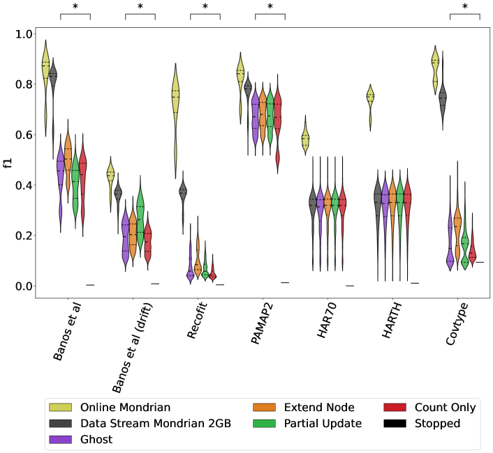
Figure 3: Comparison of out-of-memory strategies for the real datasets (n=200 repetitions). The star annotation indicates statistically significant differences (Bonferroni corrected) between all pairs of proposed out-of-memory strategies (Ghost, Extend Node, Partial Update, Count Only, and Stopped).

3 Results

Our experiments evaluated the out-of-memory and adaptation strategies presented previously. We evaluated both sets of methods separately. Unless specified otherwise, we allocated 600 KB of memory for the forest, which allowed for 940 to 1600 nodes in the forest depending on the number of features, labels, and trees. As a comparison, the Raspberry Pi Pico has 256 KB of memory and the Arduino has between 2 KB (Uno) and 8 KB (MEGA 2560).

3.1 Baselines

Figure 3 shows the F1 score distributions obtained at the end of each dataset. The experiment includes the methods described in Section 2.3 — executed wih a memory limit of 0.6 MB — as well as the online Mondrian forest and the Data Stream Mondrian forest with 2 GB of memory for reference. The limit of 2 GB is reached for the Covtype and Recofit datasets, and the Data Stream Mondrian 2 GB method applies the Extend Node method in that situation. The Online Mondrian is the Python implementation available on GitHub mondrian_implementation_1 that we modified to output the offline F1 score.

The Online Mondrian reaches state-of-the-art performance in the real datasets StreamDM-CPP ; fast_and_slow ; kappa_updated_ensemble ; cross_subject_validation . The Data Stream Mondrian 2 GB performance is significativly lower than the Online Mondrian. These differences are explained by two factors: the Online Mondrian is evaluated with a holdout set randomly selected from the dataset whereas the Data Stream Mondrian is evaluated with a prequential method (as is commonly done in data streams); the Online Mondrian can access to previous data points while the Data Stream Mondrian cannot. The Online Mondrian is given here as a reference for comparison, however, it should not be directly compared to the Data Stream Mondrian as these methods operate in different contexts.

The Stopped method, the default reference for evaluation under memory constraints, has by far the lowest F1 score, which demonstrates the usefulness of our out-of-memory strategies. The impact of memory limitation is clear and can be seen by the substantial performance edge of Data Stream Mondrian 2 GB over the other methods.

3.2 Out-of-memory strategies

The star annotation in Figure 3 highlights statistically significant differences among the five proposed out-of-memory strategies (Ghost, Extend Node, Partial Update, Count Only, and Stopped). No significant differences are observed between the methods on the HAR70 and HARTH datasets, except for Stopped, which performs significantly lower than the others.

In the other datasets, the Extend Node method consistently stands above the other ones except for the Banos et al with drift dataset where the Partial Update method achieves the best F1 score. This is due to a faster recovery of the nodes’ counters after the drift. The Extend Node makes the best of two factors. First, it does not drop any data points compared to Partial Update or Count Only. Second, since it extends the node boxes, future data points fall within the box and receive the prediction of the corresponding leaf, whereas the Count Only and the Ghost methods soften the leaf prediction depending on the data point distance with the box.

Figure 4 depicts the F1 score distributions for 40 synthetic datasets generated with MOA. All our proposed out-of-memory strategies achieve similar F1 scores — clearly better than the default Stopped method. Additionally, no significant difference is observed between Extend Node, Partial Update, Ghost, and Count Only across these datasets. However, it is noteworthy that the Stopped method exhibits significantly lower performance compared to the other strategies.

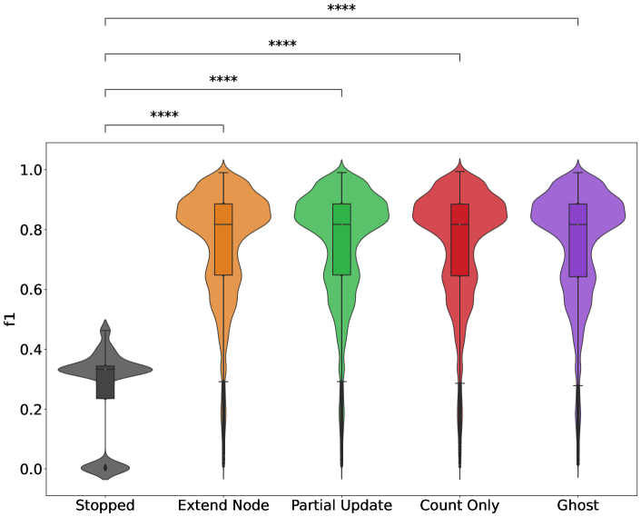
Figure 4: Comparison of out-of-memory strategies for the 40 synthetic datasets generated with MOA (n=200 repetitions).

The difference in F1 score between the Stopped Mondrian and the other methods is reported in Table 3 for the real datasets. The difference is computed for all numbers of trees and we report the minimum, the mean, and the maximum. On average, the Extend Node has the best improvement over Stopped Mondrian with an average improvement in F1-score of 0.31, a minimum of 0.1, and a maximum of 0.66.

			$\Delta$ F1
Dataset	Method Name	Min	Mean	Max
Banos et al	Count Only	.23	.42	.56
	Extend Node	.35	.49	.63
	Ghost	.24	.43	.56
	Partial Update	.26	.4	.57
Banos et al (drift)	Count Only	.07	.17	.27
	Extend Node	.09	.2	.32
	Ghost	.08	.18	.31
	Partial Update	0.13	0.26	0.4
Covtype	Count Only	.0	.05	.18
	Extend Node	.0	.13	.37
	Ghost	.0	.07	.31
	Partial Update	.0	.07	.29
HAR70	Count Only	.09	.3	.48
	Extend Node	.09	.3	.48
	Ghost	.09	.29	.48
	Partial Update	.09	.3	.48
HARTH	Count Only	.04	.3	.42
	Extend Node	.04	.3	.42
	Ghost	.04	.3	.41
	Partial Update	.04	.3	.42
PAMAP2	Count Only	.47	.64	.79
	Extend Node	.53	.66	.77
	Ghost	.53	.66	.77
	Partial Update	.53	.66	.77
Recofit	Count Only	.02	.04	.11
	Extend Node	.04	.1	.25
	Ghost	.02	.07	.22
	Partial Update	.03	.06	.16

Table 3: $\Delta$F1 score compared to Stopped Mondrian. Minimum, maximum, and average scores are computed across all tree numbers.

From these results, we conclude that the Extend Node should be the default strategy to follow when the Mondrian forest reaches the memory limit.

3.3 Concept Drift Adaptation for Mondrian Forest under Memory Constraint

Figure 5 shows the F1 score for the three proposed leaf trimming strategies. All trimming strategies were evaluated with the Extend Node out-of-memory strategy as it outperforms the other out-of-memory strategies per our previous experiment. In the case of Banos et al with drift, the random trimming method outperforms the other ones whereas for the stable datasets (Banos et al, Covtype, Recofit), no trimming appears to be the best strategy.

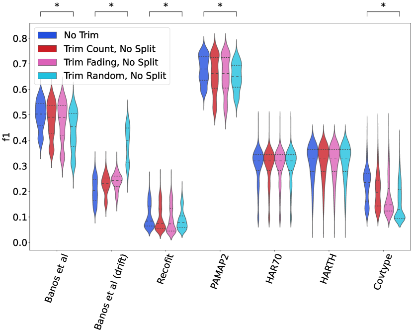
Figure 5: Comparison of node trimming strategies for the real datasets (n=200 repetitions). The star annotation indicates statistically significant differences (Bonferroni corrected).

Figure 6 shows the F1 score for the three splitting methods (no split, Split AVG, and Split Barycenter) combined with random trimming and extend node as the out-of-memory strategy. With the drift dataset, the three methods perform better than not trimming. Finally, with Banos et al, Recofit, and Covtype datasets, not trimming is generally better than randomly trimming.

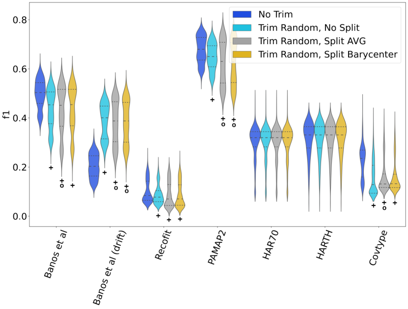
Figure 6: Comparison of node splitting strategies (n=200 repetitions). The cross below the violin indicates a statistical significant difference between, the method and No Trim, whereas the circle indicates a difference with No Split.

Figure 7 illustrates the evolution of the F1 score over time using 5-tree Mondrian forests with real datasets. We observe that the Mondrian 2GB consistently achieves a higher plateau in three of the datasets (Banos et al, Covertype, and Recofit). Additionally, the two Trim Random methods exhibit a decline in F1 score on two datasets (Banos et al and Covtype). Interestingly, all methods yield similar results with the PAMAP2, HAR70, and HARTH datasets, suggesting that the features may not adequately capture the label information.

In Figure 8, we present the F1 score’s evolution over time using 5-tree Mondrian forests with drift datasets. Notably, the Banos et al (drift) dataset experiences a sudden drift that impacts all methods, but they manage to recover, with the Trim Random methods exhibiting a faster recovery. For the RandomRBF dataset, all methods show a simultaneous drop in performance, but only the Trim Random methods demonstrate recovery from the gradual drift. Additionally, the figure includes the results for the Hyperplane datasets, where all methods perform similarly.

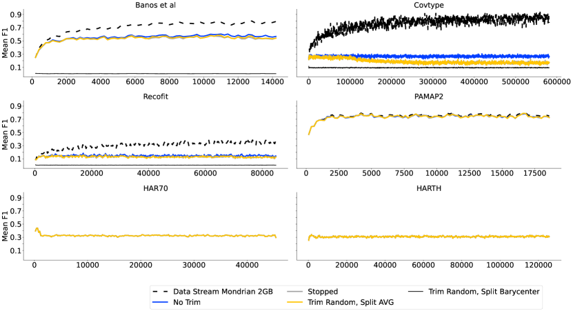
Figure 7: The Evolution of F1 score over time for a 5-Tree Mondrian forest with stable datasets (n=10 repetitions).

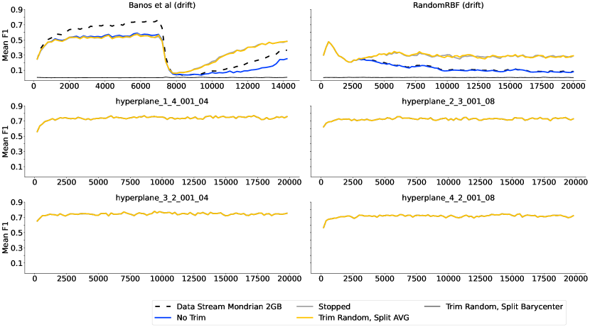
Figure 8: The evolution of F1 score over time for a 5-Tree Mondrian forest with drift datasets (n=10 repetitions).

Table 4 summarizes the delta of F1 scores of the trimming methods compared to the Stopped method. From these results, we conclude that randomly trimming allows the Mondrian forest to adapt to concept drift. We also conclude that using the split methods (Split AVG and Split Barycenter) should be the default method to grow the Mondrian trees after trimming as they exhibit a better F1 score than not splitting.

			$\Delta$ F1
Dataset	Method Name	Min	Mean	Max
Banos et al	Trim Count, No Split	.32	.48	.62
	Trim Count, Split AVG	.33	.49	.62
	Trim Count, Split Barycenter	.34	.49	.62
	Trim Fading, No Split	.29	.47	.61
	Trim Fading, Split AVG	.31	.48	.61
	Trim Fading, Split Barycenter	.3	.48	.62
	Trim Random, No Split	.25	.43	.59
	Trim Random, Split AVG	.21	.43	.59
	Trim Random, Split Barycenter	.19	.43	.6
Banos et al (drift)	Trim Count, No Split	.11	.22	.33
	Trim Count, Split AVG	.15	.28	.39
	Trim Count, Split Barycenter	.14	.28	.38
	Trim Fading, No Split	.13	.23	.33
	Trim Fading, Split AVG	.2	.38	.53
	Trim Fading, Split Barycenter	.18	.39	.52
	Trim Random, No Split	.22	.38	.52
	Trim Random, Split AVG	.19	.37	.53
	Trim Random, Split Barycenter	.17	.37	.54
Covtype	Trim Count, No Split	.0	.11	.38
	Trim Count, Split AVG	.0	.12	.37
	Trim Count, Split Barycenter	.0	.12	.37
	Trim Fading, No Split	.0	.08	.38
	Trim Fading, Split AVG	.0	.12	.39
	Trim Fading, Split Barycenter	.0	.12	.37
	Trim Random, No Split	.0	.06	.31
	Trim Random, Split AVG	.01	.07	.31
	Trim Random, Split Barycenter	.0	.07	.3
HAR70	Trim Count, No Split	.09	.3	.48
	Trim Count, Split AVG	.09	.3	.48
	Trim Count, Split Barycenter	.09	.3	.48
	Trim Fading, No Split	.09	.3	.48
	Trim Fading, Split AVG	.09	.3	.48
	Trim Fading, Split Barycenter	.09	.3	.48
	Trim Random, No Split	.09	.3	.48
	Trim Random, Split AVG	.09	.3	.48
	Trim Random, Split Barycenter	.09	.3	.48
HARTH	Trim Count, No Split	.04	.3	.42
	Trim Count, Split AVG	.04	.3	.42
	Trim Count, Split Barycenter	.04	.3	.42
	Trim Fading, No Split	.04	.3	.42
	Trim Fading, Split AVG	.04	.3	.42
	Trim Fading, Split Barycenter	.04	.3	.42
	Trim Random, No Split	.04	.3	.42
	Trim Random, Split AVG	.04	.3	.42
	Trim Random, Split Barycenter	.04	.3	.42
PAMAP2	Trim Count, No Split	.48	.64	.77
	Trim Count, Split AVG	.48	.65	.78
	Trim Count, Split Barycenter	.48	.64	.78
	Trim Fading, No Split	.47	.64	.77
	Trim Fading, Split AVG	.47	.63	.79
	Trim Fading, Split Barycenter	.47	.63	.78
	Trim Random, No Split	.5	.64	.76
	Trim Random, Split AVG	.44	.61	.77
	Trim Random, Split Barycenter	.44	.61	.77
Recofit	Trim Count, No Split	.03	.09	.26
	Trim Count, Split AVG	.04	.1	.25
	Trim Count, Split Barycenter	.04	.1	.25
	Trim Fading, No Split	.03	.09	.26
	Trim Fading, Split AVG	.03	.1	.24
	Trim Fading, Split Barycenter	.03	.1	.24
	Trim Random, No Split	.03	.08	.22
	Trim Random, Split AVG	.02	.08	.21
	Trim Random, Split Barycenter	.02	.08	.24

Table 4: $\Delta$F1 score compared to Stopped Mondrian for the trimming methods. Minimum, maximum, and average scores are computed across all tree numbers.

3.4 Impact of the Memory Limit

We note in Figures 3, 5, and 6, that the F1-scores tend to be low even though the Data Stream Mondrian 2 GB reaches state-of-the-art F1-scores. This implies that reducing the memory from 2 GB to 600 KB has a strong impact on the performance. We also note that this impact varies between datasets. For the RandomRBF stable dataset, the methods are closer to the Data Stream Mondrian 2 GB compared to the Covtype dataset where there is a more important difference.

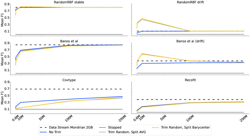
Figure 9: Evaluation of the memory impact on the top out-of-memory strategy and the top trimming methods described in Section 2.3 and Section 2.4 (n=10 repetitions). The results are shown for 50 trees.

Figure 9 shows the evolution of the memory limit impact on the F1-score for a Mondrian forest with 50 trees. We selected 50 trees as it is the number of trees that benefit the most from more memory. Indeed, more memory means they are less likely to underfit and thus, have better performance than fewer trees. Similar trends are observed with fewer trees. The dashed black line indicates the F1-score reached by Data Stream Mondrian 2 GB.

We note that, except for the Stopped method, F1-scores increase with the amount of available memory. This is explained by the fact that trees can grow more nodes and therefore describe a finer-grained partition of the feature space.

We observe that the sharpest improvement for the No Trim method happens between 600 KB and 10 MB, after which the F1-score increase slows down and plateaus toward the Data Stream Mondrian 2 GB F1-score.

The trimming methods with split exhibit two behaviors. For stable datasets, they follow the trend of No Trim. For the drift datasets, the trimming methods improve beyond the Data Stream Mondrian 2 GB up to the 10 MB limit, after which the F1-score decreases down to the Data Stream Mondrian 2 GB.

This behavior is explained by the trimming algorithm that trims based on the tree count rather than the tree size. When too much memory is allocated the size of the trees becomes too big for the trimming pace. Therefore, the old concept is not trimmed out fast enough, which explains the decrease in F1-score beyond the 10 MB mark for the trimming methods on the drift datasets.

Table 5 presents the total runtime of Trim Random with Split Barycenter and No Trim on the Banos et al dataset. The runtime is influenced by two main factors: the number of trees and the amount of available memory. It’s worth noting that the Extend Node method, due to its predictable memory access patterns, can be optimized to run faster than a Mondrian forest with trimming enabled. For instance, a Mondrian forest with 50 trees and 2GB of memory takes only 9 seconds to run with Extend Node, while it requires 442 seconds with trimming enabled.

		Memory	0.6MB	1MB	10MB	100MB	200MB
	Tree Count
	1		0.59	0.87	2.77	2.78	2.89
	5		0.78	1.03	20.35	45	44
Trim Random	10		0.91	1.15	20.12	93	91
Split Barycenter	20		0.97	1.34	20.89	185	185
	30		1.09	1.55	22.27	230	277
	50		1.25	1.82	23.97	238	442
	1		0.65	0.99	5.47	5.68	5.68
	5		0.77	1.46	25	49	51
No Trim	10		0.90	1.53	24.75	102	107
	20		1.03	1.62	23.55	201	216
	30		1.21	1.88	24.24	251	315
	50		1.53	2.32	25	251	476

Table 5: Total runtime in seconds of the Trim Random, Split Barycenter and No Trim method on the Banos et al dataset. The runtime varies depending on the number of trees used and the amount of memory available.

4 Related Work

Edge computing is a concept where processing is done close to the device that produced the data, which generally means on devices with much less memory than regular computing servers. There are many surveys about classification for edge computing survey-edge-machine-learning ; tinyML-survey-1 ; tinyML-survey-2 , but most of the work focuses on deep learning, which is not applicable in our case because it requires a lot of data and time to train the model. They discuss inherent problems related to learning with edge devices, in particular about lighter architecture and distributed training. They also depict areas where machine learning on edge devices would be impactful like computer vision, fraud detection, or autonomous vehicles. Finally, these studies draw future work opportunities such as data augmentation, distributed training, and explainable AI. Aside from the deep learning approaches, the survey in survey-edge-machine-learning discusses two machine learning techniques with a small memory footprint: the Bonsai and ProtoNN methods.

Bonsai bonzai_tree is a tree-based algorithm designed to fit in an edge device memory. It is a sparse tree that comes with a low-dimension projection of the feature space to improve learning while limiting memory usage and achieving state-of-the-art accuracy. Similarly, ProtoNN protoNN is a kNN based model that performs a low-dimension projection of the features to increase accuracy and improve its memory footprint. It also compresses the training set into a fixed amount of clusters. ProtoNN and Bonsai claim to remain below 2KB while retaining high accuracy. However, these models don’t apply to evolving data streams because their low-dimension projections and their structures are pre-trained based on existing data, thus, adjusting them would require more time and memory. Additionally, our method starts from scratch whereas ProtoNN or Bonsai require data before being used.

When it comes to forests designed for concept drift, there are many variations and many mechanisms. The Hoeffding Adaptive Tree HAT embeds a concept drift detector and grows a ghost branch when it detects a drift in a branch. The ghost branch replaces the old one when its performance becomes better. Similarly, the Adaptive Random Forest adaptive_learning_from_stream keeps a drift detector for each tree and starts growing a ghost tree when a drift is detected. The work in online_random_forest_2 presents a forest that is constantly evolving where each decision tree has its size limit. When the limit is reached, it restarts from the last created node. With this mechanism, trees with a smaller limit will adapt faster to recent data points. Additionally, the forest also embeds the ADWIN adwin concept drift detector and restarts the worst base learner when a drift is detected. This mechanism called the ADWIN bagging is used in the Adaptive Rotation Forest adaptive_rotation_forest in addition to a low-dimension projection of the features with an incremental PCA. Such combinations allow the forest to maintain the most accurate base classifiers while keeping the projection up-to-date. Our methods differ from ADWIN or the Adaptive Rotation Forest because we rely on passive drift adaptation rather than using a drift detector.

The Kappa Updated Ensemble kappa_updated_ensemble is an ensemble method that notices drifts by self-monitoring the performance of its base classifiers. In case of a drift, the model trains new classifiers. The prediction is made using only the best classifiers from the ensemble but the method never discards a base classifier as it can still be useful in the future. This mechanism of keeping unused trees raises a memory problem since it may fill the memory faster for very little benefit.

Similarly, the work in pruning_ensemble_for_evolving_streams proposes a method to prune base learners based on their global and class-wise performances. It is used to reduce memory consumption while retaining good accuracy across all classes. The method evaluates the base learners for each class then ranks them using a modified version Borda Count.

The Mean error rate Weighted Online Boosting mean_error_weighted_online_boosting is an online boosting method where the weights are calculated based on the accuracy of previous data. Even though the method is not designed for concept drift, the self-monitoring of the accuracy makes the base learner train more on recent data making the ensemble robust to concept drift.

The Robust Online Self-Adjusting Ensemble (ROSE) rose is a classifier ensemble designed for imbalanced data streams with concept drifts, where each sub-classifier is constructed using a random feature subspace with an ADWIN drift detector. In case a drift is detected, a background ensemble is trained on a class-wise sliding window, which maintains a sliding window per class thus downsampling the majority classes. After processing a thousand data points, the top sub-classifiers from both the current ensemble and the background ensemble are compared, and the best ones are selected to form the new ensemble. This process ensure the background ensemble is trained on fresh and balanced data points.

The One-Class Drift Detector (OCDD) uses an additional classifier to recognize a concepts. The classifier is trained on the first complete sliding window. From this first window, the classifier learns the distribution of the current concept and a drift is detected if the new data points contains too many outliers.

These last studies rely on ranking the base learners of the ensemble to either adjust or disable them. However, these coarse-grain approaches are memory intensive and are not applicable to the trimming methods because they would require keeping statistics for each node.

5 Conclusion

We adapted Mondrian forests to support data streams and we proposed five out-of-memory strategies to deploy them under memory constraints. Results show that the Extend Node method has the best improvement on average. With a carefully tuned number of trees, the Extend Node also has the highest F1 score gain compared to the Stopped strategy. Thus, we recommend using Extend Node as the default strategy.

We also compared node trimming methods for the Mondrian trees and there are two viable methods depending on the situation. Not trimming is the best option in most case of stable dataset. However, when expecting a concept drift, the trim Random with splits is preferable. The drawback with the Trim Random method is that it deteriorates the F1 score on stable streams.

Overall, this paper showed that using our out-of-memory strategies is critical in order to make the Mondrian forest work in a memory-constrained environment. In particular, existing Mondrian forest implementations mondrian_implementation_1 ; mondrian_implementation_2 do not have any out-of-memory strategy and will fail if they cannot allocate any more nodes. Using the Extend Node strategy allows an average F1 score gain of 0.28 accross all datasets compared to not doing anything. Similarly, using Trim Random offers an average F1 score gain of 0.3.

Our results show no significant difference between the two types of node splitting strategy. By default, we would recommend using Split AVG because it is less compute-intensive.

Future work will investigate trim mechanisms to adaptively trim depending on the memory limit and concept drift. Finally, we suggest exploring the use of drift detectors such as ADWIN adwin to switch between No Trim and Trim Random.

Compliance with Ethical Standards

This work was funded by a Strategic Project Grant of the Natural Sciences and Engineering Research Council of Canada. The computing platform was obtained with funding from the Canada Foundation for Innovation. The authors have no conflicts of interest.

References

- (1) Balaji Lakshminarayanan. Python implementation of the mondrian forest, 2014.
- (2) Oresti Banos, Juan-Manuel Galvez, Miguel Damas, Hector Pomares, and Ignacio Rojas. Window Size Impact in Human Activity Recognition. Sensors, 14(4):6474–6499, apr 2014.
- (3) Albert Bifet and Ricard Gavaldà. Learning from Time-Changing Data with Adaptive Windowing. In Proceedings of the 2007 SIAM International Conference on Data Mining. Society for Industrial and Applied Mathematics, apr 2007.
- (4) Albert Bifet and Ricard Gavaldà. Adaptive Learning from Evolving Data Streams. In Advances in Intelligent Data Analysis VIII, pages 249–260. Springer Berlin Heidelberg, 2009.
- (5) Albert Bifet and Ricard Gavaldà. Adaptive learning from evolving data streams. In Advances in Intelligent Data Analysis VIII, pages 249–260. Springer Berlin Heidelberg, 2009.
- (6) Albert Bifet, Geoff Holmes, Richard Kirkby, and Bernhard Pfahringer. MOA: Massive Online Analysis. Journal of Machine Learning Research, 11(May):1601–1604, 2010.
- (7) Albert Bifet, Geoff Holmes, Bernhard Pfahringer, Richard Kirkby, and Ricard Gavaldà. New ensemble methods for evolving data streams. In Proceedings of the 15th ACM SIGKDD international conference on Knowledge discovery and data mining - KDD '09. ACM Press, 2009.
- (8) Albert Bifet, Jiajin Zhang, Wei Fan, Cheng He, Jianfeng Zhang, Jianfeng Qian, Geoff Holmes, and Bernhard Pfahringer. Extremely Fast Decision Tree Mining for Evolving Data Streams. Proceedings of the 23rd ACM SIGKDD International Conference on Knowledge Discovery and Data Mining - KDD ’17, pages 1733–1742, 08 2017.
- (9) Alberto Cano and Bartosz Krawczyk. Kappa updated ensemble for drifting data stream mining. Machine Learning, 109:175–218, 01 2020.
- (10) Alberto Cano and Bartosz Krawczyk. ROSE: Robust Online Self-Adjusting Ensemble for Continual Learning on Imbalanced Drifting Data Streams. Machine Learning, 111(7):2561–2599, 2022.
- (11) Akbar Dehghani, Omid Sarbishei, Tristan Glatard, and Emad Shihab. A quantitative comparison of overlapping and non-overlapping sliding windows for human activity recognition using inertial sensors. Sensors, 19(22), 2019.
- (12) Dr. Lachit Dutta and Swapna Bharali. Tinyml meets iot: A comprehensive survey. Internet of Things, 16:100461, 2021.
- (13) Sanem Elbasi, Alican Büyükçakır, Hamed Bonab, and Fazli Can. On-the-fly ensemble pruning in evolving data streams, 09 2021.
- (14) João Gama, Raquel Sebastião, and Pedro Pereira Rodrigues. Issues in Evaluation of Stream Learning Algorithms. Proceedings of the 15th ACM SIGKDD International Conference on Knowledge Discovery and Data Mining, page 329–338, 2009.
- (15) Chirag Gupta, Arun Sai Suggala, Ankit Goyal, Harsha Vardhan Simhadri, Bhargavi Paranjape, Ashish Kumar, Saurabh Goyal, Raghavendra Udupa, Manik Varma, and Prateek Jain. ProtoNN: Compressed and accurate kNN for resource-scarce devices. In Doina Precup and Yee Whye Teh, editors, Proceedings of the 34th International Conference on Machine Learning, volume 70 of Proceedings of Machine Learning Research, pages 1331–1340. PMLR, 06–11 Aug 2017.
- (16) HelloAlone. C++ implementation of the mondrian forest, 2018.
- (17) Nagaraj Honnikoll and Ishwar Baidari. Mean error rate weighted online boosting method. The Computer Journal, 10 2021.
- (18) Martin Khannouz and Tristan Glatard. A benchmark of data stream classification for human activity recognition on connected objects. Sensors (Basel, Switzerland), 20, 2020.
- (19) Martin Khannouz, Bo Li, and Tristan Glatard. OrpailleCC: a Library for Data Stream Analysis on Embedded Systems. The Journal of Open Source Software, 4:1485, 07 2019.
- (20) Ashish Kumar, Saurabh Goyal, and Manik Varma. Resource-efficient machine learning in 2 kb ram for the internet of things. In Proceedings of the 34th International Conference on Machine Learning - Volume 70, ICML’17, page 1935–1944. JMLR.org, 2017.
- (21) Balaji Lakshminarayanan, Daniel M Roy, and Yee Whye Teh. Mondrian Forests: Efficient Online Random Forests. In Z. Ghahramani, M. Welling, C. Cortes, N. D. Lawrence, and K. Q. Weinberger, editors, Advances in Neural Information Processing Systems 27, volume 4, pages 3140–3148. Curran Associates, Inc., jun 2014.
- (22) Aleksej Logacjov, Kerstin Bach, Atle Kongsvold, Hilde Bremseth Bårdstu, and Paul Jarle Mork. HARTH: A Human Activity Recognition Dataset for Machine Learning. Sensors, 21(23):7853, November 2021.
- (23) Jacob Montiel, Albert Bifet, Viktor Losing, Jesse Read, and Talel Abdessalem. Learning Fast and Slow: A Unified Batch/Stream Framework. In 2018 IEEE International Conference on Big Data (Big Data). IEEE, dec 2018.
- (24) Dan Morris, T. Scott Saponas, Andrew Guillory, and Ilya Kelner. RecoFit: Using a Wearable Sensor to Find, Recognize, and Count Repetitive Exercises. In Proceedings of the SIGCHI Conference on Human Factors in Computing Systems, CHI ’14, page 3225–3234, New York, NY, USA, 2014. Association for Computing Machinery.
- (25) Dan Morris, T. Scott Saponas, Andrew Guillory, and Ilya Kelner. RecoFit: Using a Wearable Sensor to Find, Recognize, and Count Repetitive Exercises, 2014.
- (26) M. G. Sarwar Murshed, Christopher Murphy, Daqing Hou, Nazar Khan, Ganesh Ananthanarayanan, and Faraz Hussain. Machine learning at the network edge: A survey. ACM Comput. Surv., 54(8), oct 2021.
- (27) Partha Pratim Ray. A review on tinyml: State-of-the-art and prospects. Journal of King Saud University - Computer and Information Sciences, 2021.
- (28) Attila Reiss and Didier Stricker. Introducing a New Benchmarked Dataset for Activity Monitoring. In 2012 16th International Symposium on Wearable Computers, pages 108–109, 2012.
- (29) Yu Sugawara, Satoshi Oyama, and Masahito Kurihara. Adaptive rotation forests: Decision tree ensembles for sequential learning. In 2021 IEEE International Conference on Systems, Man, and Cybernetics (SMC), pages 613–618, 2021.
- (30) Astrid Ustad, Aleksej Logacjov, Stine Øverengen Trollebø, Pernille Thingstad, Beatrix Vereijken, Kerstin Bach, and Nina Skjæret Maroni. Validation of an Activity Type Recognition Model Classifying Daily Physical Behavior in Older Adults: The HAR70+ Model. Sensors, 23(5):2368, January 2023.